RD-RI24 473 AVERAGE CASE

ANALYSIS OF N RDJACENCY MAP SEARCHINGTECHNIQUE(U) ILL-INOIS UNIY AT URBANA APPLIED

COMPUTATION THEORY GROUP G BILARDI DEC Bi ACT-31

UNCLASSIFIED N89014-79-C-8424 F/G 12/1 NuE~~hhiEhhmhhhhEmhhhE

EMEOMONEEhhI

1.01

II

Jill .-25 1111 .4 11.6

MICROCOPY RESOLUTION TEST CHART

*NATIONAL BUREAU Of STANDARDS- 1963-A

4~4 4

414

SECURITY CLASSIFICATION OF THIS PAGE (lWhn Date Entered) ._:~~~~~~~RA REOTDCMNATO AEW~ STRUCTIONS

REPORT DOCUMENTATION PAGE BEFORE COMPLETING FORMI. REPORT NUMBER GOVT ACCESSION NO. 3. RECIPIENT'S CATALOG NUMBER

4. TITLE (and Subtitle) S. TYPE OF REPORT & PERIOO COVEREO

AVERAGE CASE ANALYSIS OF AN ADJACENCY MAP - ihhical ReportSEARCHING TECHNIQUESA IGEN E6. PERFORMING ORG. REPORT NUMBER

R-928 (ACT-31); UILU-ENG7. AUTHOR(e) I. CONTRACT Ott GRANT NUMMER(S)

ECS-81-06939;N0001-79-C-0424

Gianfranco Bilardi

S. PERFORMING ORGANIZATION NAME ANO ADDRESS 10. PROGRAM ELEMENT. PROJECT. TASK

Coordinated Science Laboratory AREA & WORK UNiT NUMBERSUniversity of IllinoisUrbana, IL 61801

I".- CONTftON.iNo OICE MAME ANO AORESS 12. REPORT DATE

December 19811S. NUMBER oF PAGES

5614. MONITORING AGENCY NAME & AOORESS(II different from Controillng Office) IS. SECURITY CLASS. (oa this report)

UNCLASSIFIEDISo. OECLASSiFICATION/OOWNGRAOING

SCHEOULE

1S. OISTRIUTION STATEMENT (of this Report)

17. DISTRIBUTION STATEMENT (of the abstract entered In Dlock 20, if different from Report)

Approved for public release; distribution unlimited.

Il. SUPPLEMENTARY NOTES

It. KEY WORDS (Continue on reveree side if neceeary and fdenlitrf b, block number)computational geometry, adjacency map, geometric searching, average caseanalysis, point location.

1O. ABSTRACT (Cattinue on reverse side If necesary mid identify by block number),The adjacency map is a data structure (a tree) used to solve the following

problem: given a set of parallel segments in the plane and a point p, find thesegments closest to p among those intersected by the straight line through p,perpendicular to the comon direction of the segments. The search is performedin the repetitive mode, so that preprocessing is convenient.

The problem considered is a particular case of planar point location for

O o 1473 '_SECURITY CLASSIFICATION OF THIS PAGE (When Date Entered)

UNCLASSIFIEDSIRCUMITY CIASSIFICATION Of THIS PAGMl[i( Daa Voatered)

which algorithms are known (Lipton-TarJan, Kirkpatrick), which make use of dataS structures constructed in time O(nlogn), searched in time O(logn), and stored

in space 0(n). Though asymptotically optimal, the previous algorithms are notvery practical. More practical algorithms have been proposed (Preparata,Preparata-Lipski), which use 0(nlogn) space.

In this thesis a modification of these algorithms is presented for theadjacency map, and the worst case analysis is performed.

The technique is easily extensible to general planar graphs. It isconjectured that, under reasonable assumptions on the input distribution, thenew algorithm takes expected linear storage.

A probabilistic analysis substantiates such conjecture in the case of theadjacency map, for a wide class of input distributions. In particular, whenthe segments have independent endpoints, it is shown that the number of nodes inthe corresponding adjacency map is about 6 times the number of segments. Theresults of the analysis have been confirmed by simlation.

99CURIY CLASSIFICATION Of THIS PA@E(Wben 0ma Enter**

12%%

AVERAGE CASE ANALYSIS OF AN ADJACENCY

MAP SEARCHING TECHNIQUE

- BY

GIANFRANCO BILARDI

Laur., UniversitA di. Padova, 1978

THEBSIS

Submitted in par tal t lfillmnt of the requirementsfor the degree of' Ia tei ~L~ience in Electrical Engineering

in the :ueaduate College of theUniversity of I11 nois at Urbana-Champaign, 1982

__ii

Accession For

NTIS GRA&1DTIC TAB

Urbana, Illinois

iBy

Distribuition/!

Availability CodesAvail and/or

Dist Special

[ 2

ACKNOWLEDGEMENT

I want to express my gratitude to my thesis advisor, Professor

Franco Preparata, who introduced me to Computational Geometry and provided

a very helpful guidance for this research.

Several discussions with my friend Sergio Verdu have been very useful.

This work was supported by the National Science Foundation under Grant

ECS-81-06939 and by the Joint Services Electronics Program under Contract

N00014-79-C-0424. Additional support has been provided by the International

Rotary Foundation, which granted me a Fellowship for the first year of

graduate study.

Finally, thanks to Mrs. Phyllis Young for the excellent typing of this

thesis.

p"-

U

I-

iv

TABLE OF CONTENTS

CHAPTER Page

1. INTRODUCTION .................................................. 1

2. DEFINITION AND CONSTRUCTION OF THE SEARCH TREE............... 5

3. SEARCH TREE BALANCING PROCEDURE (BALANCE)..................... 16

4. WORST CASE PERFORMANCE ANALYSIS AND STORAGE LOWER BOUNS ...... 19

-: ~5 . PROBABILISTIC ANALJYSIS . .. .. . .. .. ... ........... .. . .... . .. . .. 25

5.1. Random Model ........................................ .... 255.2. The Goals of the Analysis: Space and Time ............... 305.3. Principal Slabs and Principal Medians ................... 315.4. Mean Value of c o 3.......................3

5.5. Analysis of Rectangles in Principal Slabs ............... 365.6. Bounds for E[c(U)] ...................................... 435.7. Independent Generators: Numerical Results and

Simulations ............................... 495.8. Average Time ................................ .......... 51

6 . CONCLUSIONS .............. .. ................... . . .. .. . .... 53

REFERENCES.................................................... 56

IR

**

- ------

ABSTRACT

The adjacency map is a data structure (a tree) used to solve the

* . following problem: given a set of parallel segments in the plane and a

point p, find the segments closest to p among those intersected by the

3straight line through p, perpendicular to the common direction of the

segments. The search is performed in the repetitive mode, so that

preprocessing is convenient.

The problem considered is a particular case of planar point location

for which algorithms are known (Lipton-TarJan, Kirkpatrick), which make use

of data structures constructed in time 0(nlogn), searched in time O(logn),

and stored in space 0(n). Though asymptotically optimal, the previous

*. algorithm are not very practical. More practical algorithms have been

proposed (Preparata, Preparata-Lipski), which use 0(nlogn) space.

In this thesis a modification of these algorithms is presented for

-. the adjacency map, and the worst case analysis is performed.

The technique is easily extensible to general planar graphs. it is

"* conjectured that, under reasonable assumptions on the input distribution, the

new algorithm takes expected linear storage.

A probabilistic analysis substantiates such conjecture in the case of

the adjacency map, for a wide class of input distributions. In particular,

when the segments have independent endpoints, it is shown that the nmber of

nodes in the corresponding adjacency map is about 6 times the number of

segments. The results of the analysis have been confirmed by sinulation.

1. INTRODUCTION

The adjacency map (AM), a data structure suitable for searching a set

-q of parallel segments in the plane, has been shown to be efficiently

applicable to the solution of several problem of planar computational

geometry (1]. The AM solves the following problem: given a set 0 of

parallel segments in the plane and a point p, find the segments closest to p

among those intersected by the straight line passing through p and perpen-

dicular to the comon direction of the segments. In the sequel we assume

* ithe y axis of the Cartesian plane to be parallel to the segments. If through

each endpoint w of each member of A we trace a horizontal half-line to the

right and one to the left and we make such lines terminate when they meet

. another segment or continue to the infinity otherwise, we partition the plane

into regions. Two of these regions are half planes and all the other are

. rectangles, possibly unbounded in one or both horizontal directions. Each

rectangle is an equivalence class of points of the plane with respect to

their horizontal adjacency to vertical segments, and can be called adjacency

region.

The foregoing problem is a special case of point location in a planar

subdivision and therefore can be handled by one of the general techniques for

-. such problem [2,3,4,51.

By using a method recently developed in [31, Lipski and Preparata (11

have given an efficient algorithm for point location in the adjacency regions.

They make use of a static data structure that they call adjacency map, which

can be searched in time O(logn), constructed in time O(nlogn), and stored

14 } in space O(nlogn), where n -1g is the number of segments.

J:.,•1 -°

, v' " .' "

. I. . . . - .. / . . /_ . . •- .. . - . - . , . -. -: - '

2

The reason to further consider the problem stems from a theoretical

result due to Lipton and TarJan (4], and Kirkpatrick [51 who showed that

O(logn) searching time and 0(nlogn) preprocessing time can be achieved with

a data structure which only uses O(n) space. Even though the Lipton-Tarjan

method is algorithmically extremely complicated (no conclusion to the

contrary is available for Kirkpatrick's method), it suggests that a practical

algorithm may exist with the same performance.

In this thesis we consider a new algorithm for the AM, which is a

conceptually simple modification of the algorithm presented in (1]. While

the worst case asymptotic performance is the same as in [1], the average

performance is improved. We show that if the segments are independent of

each other, under some very weak assumptions, expected linear storage is

achieved, and also that except for a presorting operation, the algorithm runs

in expected linear time. We also make use of a procedure different from the

one used in (1,2] to balance the search tree. The new procedure is simpler

and faster. Due to the nature of the procedure for building the search tree,

the bound to the depth of the tree is also reduced from F5 logn] to

3 logn + 7.

The thesis is organized as follows. In Section 2 the search tree is

defined together with a recursive procedure for constructing it, and Section

3 describes the balancing of the search tree. The worst case asymptotic

analysis is performed in Section 4. Section 5 is devoted to the probabilistic

analysis and is the main contribution of this thesis. We begin with the

definition of a suitable random model for the input of the algorithm. In

this model a segment is defined by two random variables U and V, called

generators, which are the (unordered) segment endpoints. A segment is

.-

3

statistically described by the joint distribution of its generators. We

also assume that different segments are statistically independent from each

-. other. We show that, under this assumption, the statistical properties of

the algorithm are independent of the first order generator distribution and

q they are only affected by the correlation properties of the endpoints.

Therefore there is no loss of generality in considering uniform generators.

The analysis we carry out shows that, for a broad class of generator

joint-distributions, the average number of nodes in the search tree is

linear in the number of segments. Numerical results are obtained for the

particular case of independent endpoints. For this case we get a theoretical

upper-bound of 6.07 n for the number S of nodes in the tree. Simulation

completely agrees with this upper-bound and gives an average number of nodes

close to 5.7 n. These results are very satisfactory, since it can be shown

that the search tree must contain at least 3n nodes, and therefore the

algorithm performs on the average, within a factor 2 of the absolute lower

bound. Moreover the average result for this algorithm is particularly

meaningful since - due to the law of large-numbers - the actual values

obtained for inputs of reasonably large size (say over 300) are very close

to the expected values.

,.-. The AM solves several problems related to collections of parallel

segments in the plane. Some of these problem are the Nontrivial-Contour,the External-Contour, the Point-Location, and the _oute-in-a-aze, which

are defined and discussed in (1]. These and probably several other

problems of simiLlar type arise in diverse fields of application such as

computer aided design, large-scale-integration, operation research, data

base concurrency control, etc. Of course all of the foregoing problems will

* take advantage of an efficient algorithm for the AM.

4

However we think that the implications of the present study may b .

wider. The algorithm that we present is in fact immediately extensible

to the problem of point location in a general straight-line planar

subdivision and intuition suggests that its performance will be satisfactory

in the general case. But a rigorous proof of such a statement is not

straightforward and we hope to perform such a task in future work.

L

5

* 2. DEFINITION AND CONSTRUCTION OF THE SEARCH TRIEE

We recall here from [11 the definition of the AM. The AM is a binary

tree 3C with two types of nodes having a different typographical representation:

"va V-node or "horizontal node", is associated with a horizontal line y -c

and has the ordinate c as a discriminator; "10", an 0-node or segment node,

is associated with a straight line segment on the line x -d and has the

abscissa d as discriminator.

To search for a given point p - (xy) corresponds to tracing a path in 3c

from the root to a leaf. The discriminator is compared against y for V-nodes

and against x for 0-nodes. The path makes a turn to the left when the point

coordinate is smaller than the discriminator and to the right otherwise.

* Along the path the largest abscissa smaller than x, and the smallest abscissa

larger than x, initialized to -aand -t respectively, are recorded and give,

3 when a leaf is reached, the left and the right adjacent segments, with an

* infinite abscissa corresponding to the case of no adjacent segment.

Several different search trees are possible for the same set of segments.

3 We are particularly interested in bounding the depth of the tree (to bound the

query time) and the total number of nodes (to bound the storage). The latter

* objective is the minimization of the number of nodes in the tree having the

- same horizontal or vertical discriminator. The former objective requires

instead a suitable balancing strategy when constructing the tree.

The complete definition of the AM is given by specifying the algorithm

Li

that constructs it. To describe both the Lipsi-Preparata and the present

algorithm let us introduce some definitions. A slab [B.T], with B < T, is

*the strip of plane contained between the lines y B and Y -T. A vertical

6

segment s - (X;Y1,Y2) spans slab [B,T] if Y15 B, T-- Y2 " Given a slab

[B,T] and a sequence Q of vertical segments sorted according to increasing

- abscissa and having a nontrivial intersection with the slab, the spanning

segments of Q partition the slabs into a set of regions, which we technically

call rectangles (these regions are actual rectangles, possibly unbounded on

one or both sides).

The philosophy of the AM is the following. Once a point has been located

within a slab, comparisons against the spanning segments of the slab locate

the point in a rectangle. The rectangle is then sliced in two slabs by some

line y - M, with B < M < T; a comparison against M locates the point in one

of these slabs and from there on the search proceeds recursively in the same

fashion. The search terminates when the rectangle examined is empty.

The foregoing ideas naturally suggest a recursive procedure for building

the tree in which two main steps remain to be specified: (i) how to choose M

in a given rectangle (choice of the cut point); (ii) how to organize in a

binary tree the O-nodes corresponding to a segment spanning the slab and

the 7-nodes corresponding to cut points in the rectangles. We shall describe

step (i) in this section and step (ii) in the next one.

The choice of the cut point constitutes the main difference between the

old and the new versions of the AM. In [1] the cut point is M - L(B +T)/2j

for each rectangle in the slab [B,TI. We propose instead to select M as

the median of the ordinates of all the segment endpoints following in the

rectangle. This choice is aimed at decreasing the numbers of both vertical

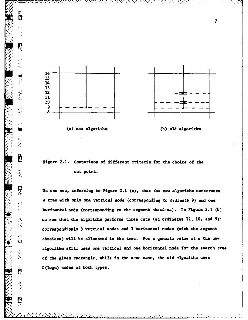
and horizontal nodes. As an example, consider a rectangle in the slab

[n/2,n] containing only one segment endpoint, say n/2+ 1, the other endpoint

being in slab [n,2n]. The situation is illustrated in Figure 2.1 for n-16.

V -

.:- ,, -. :-,

7

16151413121110S9 -- ---- -------

* (a) new algorithm (b) old algorithm

Figure 2.1. Comparison of different criteria for the choice of the

cut point.

We can see, referring to Figure 2.1 (a), that the new algorithm constructs

a tree with only one vertical node (corresponding to ordinate 9) and one

* '

... "horizontal node (corresponding to the segment abscissa). In Figure 2.1 (b)

we see that the algorithm performs three cuts (at ordinates 12, 10, and 9);

correspondingly 3 vertical nodes and 3 horizontal nodes (with the segment

abscissa) will be allocated in the tree. For a generic value of n the new

algorithm still uses one vertical and one horizontal node for the search tree

of the given rectangle, while in the same case, the old algorithm uses

O(logn) nodes of both types.

; -.- .

8

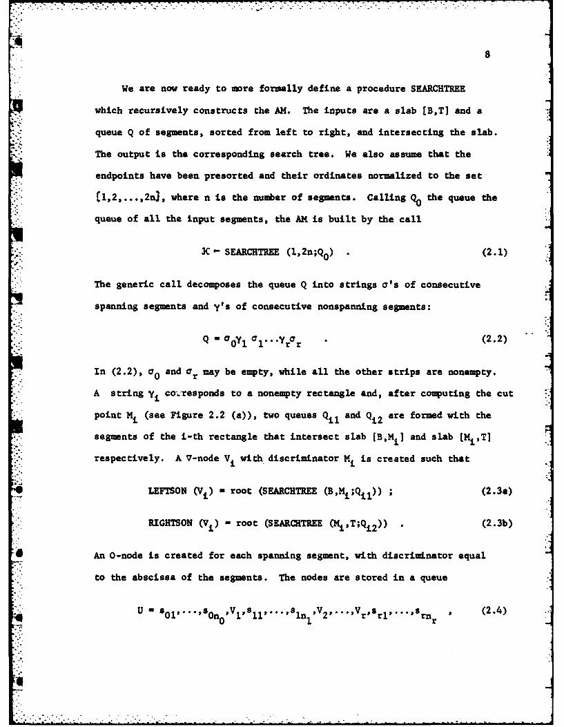
We are now ready to more formally define a procedure SEARCHTREE

which recursively constructs the AM. The inputs are a slab [B,T] and a

queue Q of segments, sorted from left to right, and intersecting the slab.

The output is the corresponding search tree. We also assume that the

endpoints have been presorted and their ordinates normalized to the set

C1,2,...,2n), where n is the number of segments. Calling Q the queue the

queue of all the input segments, the AM is built by the call

X - SEARCHTREE (1,2n;Qo) . (2.1)

The generic call decomposes the queue Q into strings a's of consecutive

spanning segments and y's of consecutive nonspanning segments:

Q a 0 y O...yr (2.2)

In (2.2), a0 and Or may be empty, while all the other strips are nonempty.

A string yi cozresponds to a nonempty rectangle and, after computing the cut

point Mi (see Figure 2.2 (a)), two queues Qil and Qi2 are formed with the

segments of the i-th rectangle that intersect slab [B,Mi] and slab [Mi,T ]

respectively. A V-node V with discriminator Mi is created such thatN ir NroE i

LEFTSON (Vi) - root (SEARCHTREE (B,M;Qil)) . (2.3a)

." E~IGHTSON (Vi) root (SEARCHITREE (Mi,Tq2) . (2.3b)

An 0-node is created for each spanning segment, with discriminator equal

to the abscissa of the segments. The nodes are stored in a queue

U " 0O', .... , V......,s , (2.4)0 1 r

9

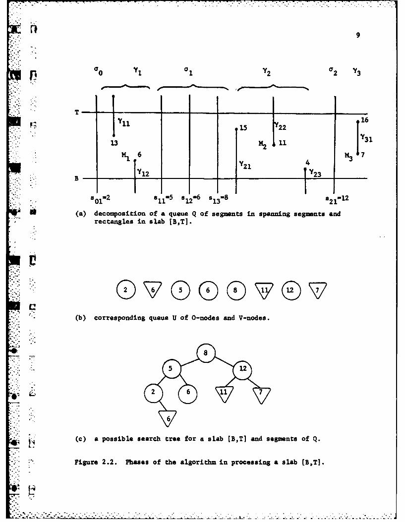
0 01 02a2 Y3

1711y 16

M 1 M6

U(a) decomposition of a queue Qof segments in spanning segments andrectangles in slab [B,TI.

(b) corresponding queue U of 0-nodes and V-nodes.

. (c) a possible search tree for a slab (B,T] and segments of Q

Figure 2.2. Phases of the algorithm in processing a slab [B,TI.

10

(see Figure 2.2 (b)). Once the queue U is completed, it is restructured

into a balanced tree U by the procedure BALANCE to be described in the

next section (see Figure 2.2 (c)).

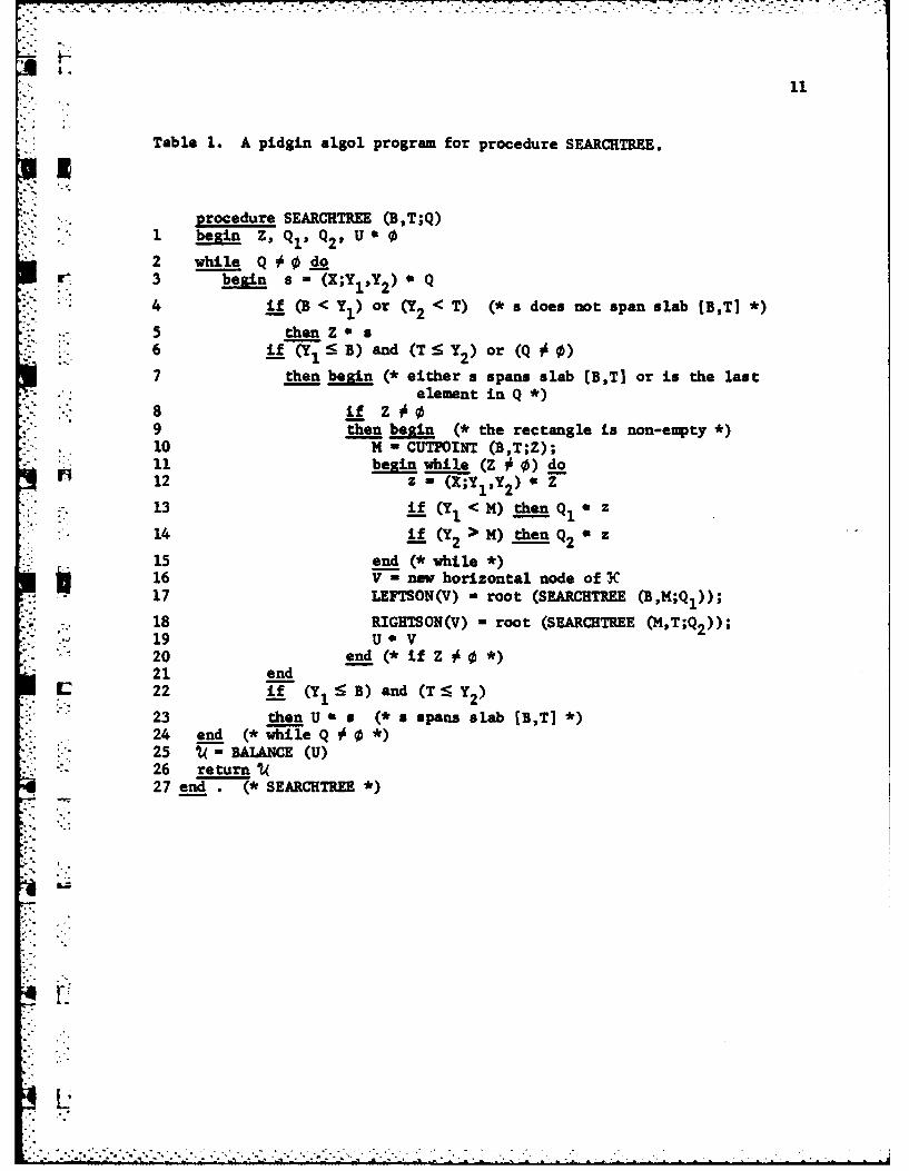
A pidgin algol program for procedure SEARCHTREE is given in Table 1.

Q Q 1 1 Q29 U, Z are queues; s Q and Q s denote the operation

POP s from Q and PUSH a into Q respectively. Queue Z is used to temporarily

store the segments contained in a rectangle. The subroutine CUTPOINT

computes the ordinate M at which we slice the rectangle. When M is known

the queues Q1 and Q2 of the segments that intersect the lower and upper

slabs, in which the rectangle is divided, can be formed. We notice that

in the Lipski-Preparata algorithm, M = L(B + T)/2J does not depend on

which segments are in the rectangle and therefore queues Q1 and Q2 may be

directly formed without using queue Z (compare with [3],[1]). This is not

the case for our version of the algorithm, in which CUTPOINT computes a

median of the endpoints within the rectangles.

To find the median of the points inside a given rectangle a standard

median algorithm [6] can be used, which will work in time linear in the

- number of points. Another solution, probably faster and easier to implement,

can be obtained by a simple modification of the procedure SEARCHTREE. The

idea is to maintain together with the queue Q of the segments, a list P of

their endpoints contained in the slab, sorted by increasing ordinate.

a1 Each segment of Q has pointers to its endpoints, when they are in P; the

pointers are null otherwise. In a first scan of Q, rectangles are formed

and points of P are marked with the name of the rectangle to which they

belong. In a second scan, a list Pi of sorted points is easily built for

I°

Table 1. A pidgin algol program for procedure SEARCHTREE.

procedure SEARCHTREE (BT;Q)1 begin Z, Ql'Q 2 U 02 while Q 0 do

r 3 begin s - (X;Y1 ,Y2) * Q

4 if (B < Yl) or (Y2 < T) (* s does not span slab (B,T] *)

5 then Z s6 if (Yl < B) and (T Y2 ) or (Q #0)7 then begin (* either s spans slab [B,T] or is the last

element in Q *)8 if Z 0 09 then besin (* the rectangle is non-empty *)

.. 10 M = CUTPOINT (B,T;Z);11 begin while (Z # 0) do12 z - (X;YlY) Z

13 if (Y < M) then Q, z

14 if (Y2 > M) thenQ2 * z

15 end (* while *)16 V - new horizontal node of3C17 LEFTSON(V) - root (SEARCHTREE (B,M;Q1 ));18 RIGHTSON(V) = root (SEARCHTREE NT;Q2));19 U V20 end (*if Z *)21 end

12 22 if (Y 1 - B) and (TS <Y 2 )

23 then U" s (* a spans slab [B,T] *)24 end (*while Q *)25 A- BALANCE (U)26 return 1(27 end . (* SEARCHTREE *)

... .. ."-. . ...

7 . . . . . . . . . . .. . .. . .

12

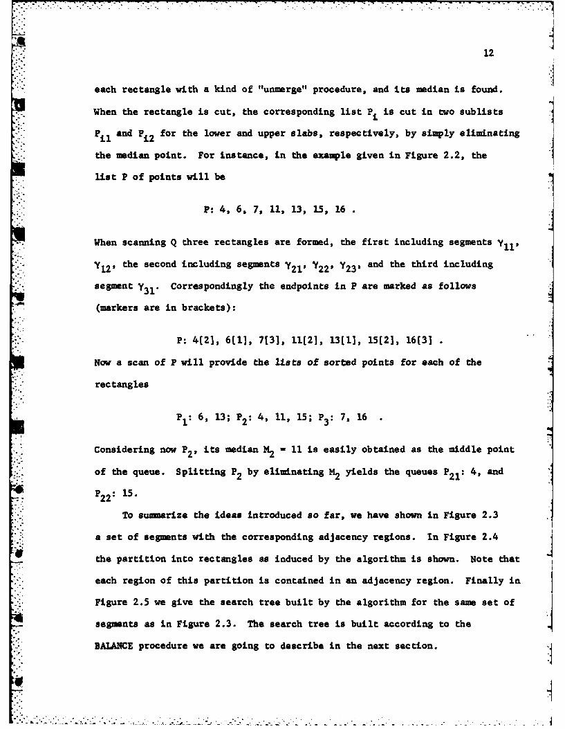
each rectangle with a kind of "unmerge" procedure, and its median is found.

When the rectangle is cut, the corresponding list Pt is cut in two sublists

P and for the lower and upper slabs, respectively, by simply eliminating

- .the median point. For instance, in the example given in Figure 2.2, the

._ list P of points will be

P: 4, 6, 7, 11, 13, 15, 16

When scanning Q three rectangles are formed, the first including segments y

S121 the second including segments Y2 1 9 y 2 2 , Y2 3 * and the third including

segment y3 . Correspondingly the endpoints in P are marked as follows!31(markers are in brackets):

P: 4[2], 6(1], 7[31, 11[21, 13(11, 15[21, 16(31

Now a scan of P will provide the lists of sorted points for each of the

rectangles

P1: 6, 13; P2 : 4, 11, 15; P3: 7, 16

Considering now P2 , its median 2 - 11 is easily obtained as the middle point

of the queue. Splitting P2 by eliminating M2 yields the queues P2 1 : 4, and

P22 : 15.

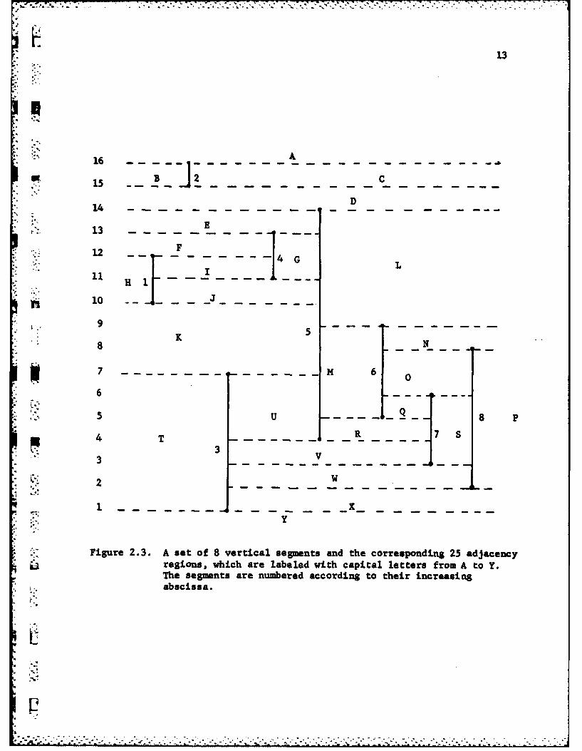
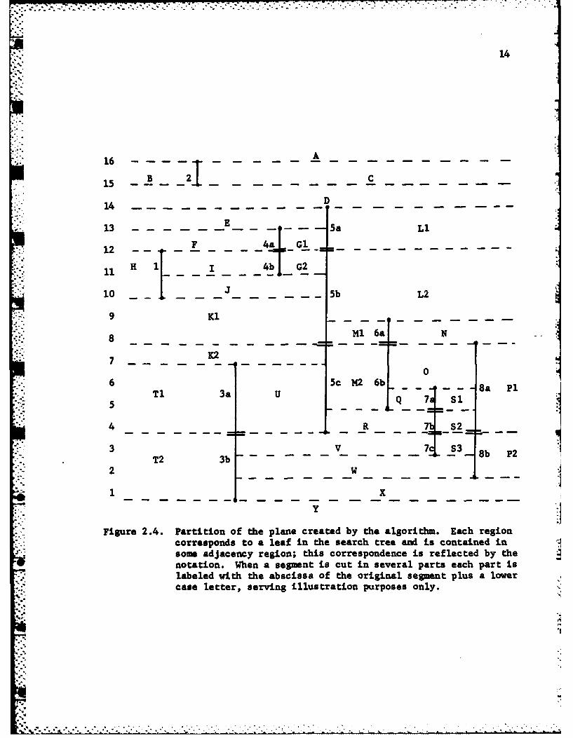
To summarize the ideas introduced so far, we have shown in Figure 2.3

a set of segments with the corresponding adjacency regions. In Figure 2.4

the partition into rectangles as induced by the algorithm is shown. Note that

each region of this partition is contained in an adjacency region. Finally in

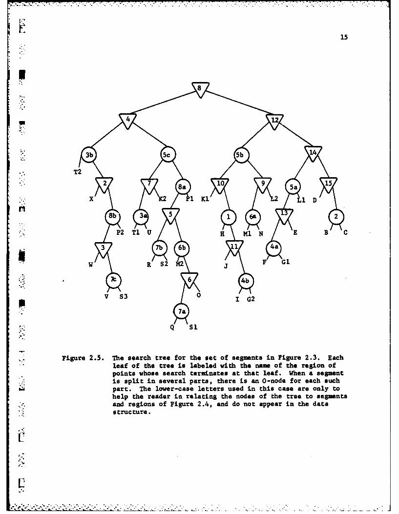
Figure 2.5 we give the search tree built by the algorithm for the same set of

segments as in Figure 2.3. The search tree is built according to the

BALANCE procedure we are going to describe in the next section.

-- + ..... .-. +, .. ,. : ++ . - ---.-.-.-.- p+ -.i° --- "-i .- --.- --: .-. .. . .. . . . - + . " .

13

16 A

-15 B J 2 C

14D

13-1

12 -

I

11 - L

10

8 ;. 5 N5

7-------- - 6 0

6

5 - FUL 8 P33

2 D

Y

Figure 2.3. A set of 8 vertical segments and the corresponding 25 adjacencyregions, which are labeled with capital letters from A to Y.The segments are numbered according to their increasingabscissa.

L:"

13 -- --.-.. -- -5a L1

14

16 - - A - - - - - - - - - -

15 B -2 -

D

13 E 5a Li

12 F 4a =4

12 -

J10 _- ---- 5b L2

9 KI

8 Ml 6a N

7 K2

06 3aU5c M2 6b8a P

']. 8 _-_8__ P=

T 3a U QS

5

T2 3b -t -

2 w

- - - - - -

Figure 2.4. Partition of the plane created by the algorithm. Each regioncorresponds to a leaf in the search tree and is contained insome adjacency region; this correspondence is reflected by thenotation. When a segment is cut in several parts each part islabeled with the abscissa of the original segment plus a lowercase letter, serving illustration purposes only.

V,

15

p8

411

T2G

xi 1-i2

P2 T/ Uu lN

V S3 0 1 iG2

,:+Q Sl

Figure 2.5. The search tree for the set of segments in Figure 2.3. Each

" leaf of the tree is labeled with the name of the region of

points whose search terminates at that leaf. When a segmentis split in several parts, there is an O-node for each suchpart. The lower-case letters used in this case are only tohelp the reader in relating the nodes of the tree to segmentsand regions of Figure 2.4, and do not appear in the datastructure.

12.'-

16

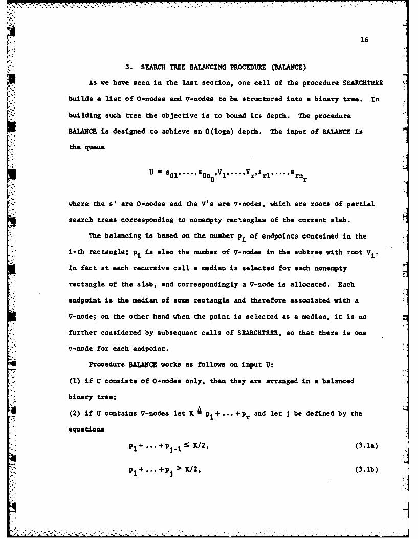
3. SEARCH TREE BALANCING PROCEDURE (BALANCE)

As we have seen in the last section, one call of the procedure SEARCHTREE

builds a list of O-nodes and V-nodes to be structured into a binary tree. In

building such tree the objective is to bound its depth. The procedure

BALANCE is designed to achieve an O(logn) depth. The input of BALANCE is

the queue

SO1, , S~no,V 1 ,..,V, S,ar r

U On ... r ... .o

where the s' are O-nodes and the V's are V-nodes, which are roots of partial

search trees corresponding to nonempty rectangles of the current slab.

The balancing is based on the number pi of endpoints contained in the

i-th rectangle; p1 is also the number of V-nodes in the subtree with root V V

In fact at each recursive call a median is selected for each nonempty

rectangle of the slab, and correspondingly a 7-node is allocated. Each

endpoint is the median of some rectangle and therefore associated with a

V-node; on the other hand when the point is selected as a median, it is no

further considered by subsequent calls of SEARCHTREE, so that there is one

V-node for each endpoint.

Procedure BALANCE works as follows on input U:

(1) if U consists of 0-nodes only, then they are arranged in a balanced

binary tree;

(2) if U contains V-nodes let K p1 +''" +p and let J be defined by ther

equations

Pl + +P-1 K/2, (3.1a)

PI + + PJ > K/2, (3.lb)

. -

"- -: ':,.'-;-;.-:'. ; . :.''':' : ',,. .:-- :- ". -. - . o , .: - :i -

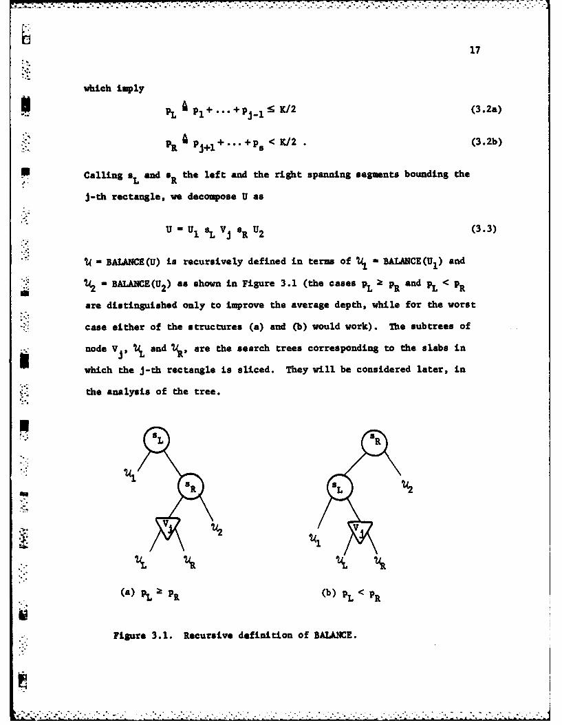
17

which imply

• + ' + P K1 X/2 (3.2a)

p 1 + < K/2 (3.2b)

Calling eL and sR the left and the right spanning segments bounding the

J-th rectangle, we decompose U as

u U L VI 5R U2 (3.3)

14 BALANCE(U) is recursively defined in terms of V, BALANCE(U 1 ) and

2 - BALANCE(U 2 ) as shown in Figure 3.1 (the cases pL PR and PL < PR

are distinguished only to improve the average depth, while for the worst

case either of the structures (a) and (b) would work). The subtrees of

node Vi, V( and N4, are the search trees corresponding to the slabs in

which the J-th rectangle is sliced. They will be considered later, in

the analysis of the tree.

LL R

RV V

(a) PL • PR, (b) PL < PPR

Figure 3.1. Recursive definition of BALAINCE.

18

In order to implement the balancing efficiently, a vector can be usedk

to store the numbers E pi, k W h,...,r. While this technique requiresi-1

O(r) time at the beginning, it allows us to find the node V in time

logarithmic in the number of V-nodes involved in each recursive call of

BALANCE. If there are only O-nodes, it is also clear that they can be

balanced in time linear in their number. In conclusion the BALANCE runs in

time linear in the total number of nodes of the input queue U.

-j

b, 4

19

4. WORST CASE PEFORMANCE ANALYSIS AND STORAGE LOWER BOUNDS

U In this section we analyze the. worst case asymptotic performance of the

method, considering the time to build the search tree (preprocessing time),

the number of nodes (storage) and the depth of the tree (search time) and

W. showing that they are O(nlogn), O(nlogn) and O(logn) respectively. In the

last part of the section we introduce lower bound considerations for

storage, which will be used in the next section for an appraisal of the

results of the probabilistic analysis of the number of nodes.

We begin by proving a lem-a showing that the number of segments and

and the number of points, either in a rectangle or in a slab, are of the

same order.

Lenna 4.1. Let eR and P be respectively the numbers of segments and

points in a rectangle, and eS and pS the same quantities in a slab

generated by the algorithm. We have pR - G(eR), and pS - 6(es).Proof. In a rectangle there are no spanning segments and therefore each

segment has at least one endpoint inside the rectangle; on the other hand

i a segment has at most two endpoints, hence eRS PR < 2 eR, which proves

PR = e(eR ). Let us now consider a slab obtained by horizontally cutting

a rectangle at the median of the segment endpoints. If p is odd both the-Rlower and upper slabs contain Ps = (PR"1)/2 points. If PR is even one

slab contains PR/2 and the other PR/2-1 points. In any case

SPR/2"-5 PS !- PR/2 so that PS - 9(p ) = 8(eR). Since a segment in the

rectangle may generate at most a segment in a slab, eS eR

Moreover, the number of segments in the slab is at least one half of the

*. *~: number of points, hence e > psi2 Z (PR/2-1)/2. Therefore (PR/4- )S eS<5 PR,

and es = e(PR). But we have seen that pS = 6 (eR), hence pS 8 B(es). C

• - i . . - . . . . . . _ . , . .:.,.:.,

20

Lemma 4.1 is useful because it shows that, in the asymptotical

analysis, the work done by the algorithm in a slab or in a rectangle can be

changed indifferently to the points or the segments. We now analyze

separately the three performance measures.

Preprocessing time. We note that each point belongs at most to O(logn)

slabs. In fact each call of the procedure SEARCHTREE processes no more than

half of the number of points processed by the calling procedure. Also we

note that at each call the work done to prepare subsequent calls is linear

in the number of points (or segments) processed. In fact, a constant work

is required for each segment to decide if it is spanning or not and, when

it is not spanning, to insert it in the queues for the lower and upper slabs

of the rectangle, if appropriate. Moreover the median of the points in each

rectangle is found in time linear in the number of points (within the rectangle),

both by using a median finding algorithm or the method proposed in Section 2.

-. The BALANCE procedure also takes time linear in the total number of tree-

nodes that it processes, and hence in the number of points of the

corresponding slab. In fact the number of spanning segments is O(e) -O(ps)

and the number r of rectangles is certainly O(ps).

In conclusion for each call 0(1) work is done for each point processed

by the call, resulting in O(nlogn) total time for the procedure SEARCHTREE,

and therefore for the entire algorithm including presorting of segments and

endpoints.

Storage. The storage is proportional to the number of nodes in the search

tree. The number of V-nodes is 2n. The number of O-nodes for each segment

is one plus the number of times the segment is cut by the median of the

same rectangle. The total number of cuts can be easily bounded considering

21

that in a rectangle of w points at most w-i segments are cut by the

Si median, and that in a rectangle with 1 and 2 points the maximum number

of cuts is 0 and 1 respectively. So the function f(w) recursively defined

by

f(l) -O, f(2) -1 ,(4.a)

f(2w) - f(w) + f(w-i) + 2w-i (4. 1b)

f(2w+l) - wf(w) + 2w , (4. lc)

is a bound for the number of cuts when processing s points. Since

f(w) = O(w log w), the total number of nodes in the tree is 0(nlogn).

Search time. This part of the analysis is somewhat delicate because the depth

8 (14 of the tree 4 - BALANCE(U) depends on the level of recursion of

SEARCHTREE in which the queue U has been formed (through the number of O-nodes

and the weight of V-nodes), and also on the way in which the nodes are arranged

in the tree. In fact, suppose a V-node V is placed at distance d (1) from

the root of u and that the subtree rooted in V has depth d2 , then 80A) 2 d I+d 2 ."

U The same is true when a subtree of O-nodes of depth d2 is formed and its

root is placed at distance d from the root of 7. These considerations lead

us to the following definition and remarks.

1) The weight of a slab is defined as K - P + .+ P"' r' and is the total

number of endpoints contained in the slab.

(1)According to standard terminology, this distance is the number of arcs

in the path from V to the root.

" :-" '- - ",; :- , ;. . .- .. : . - - _ r i • -.-'. e . .. ? ..- : - i . • , . - .- - . - - . -

- " - ' i " . "- V . -- -° " .

22

2) The number H of spanning segments in a slab of weight K is at most

K + 2. To prove this claim, we consider the rectangle whose split

generates the slab. A segment spanning the slab -mst have one

endpoint in the rectangle; this endpoint either is the cutpoint or lies

in the companion slab originating from the saze rectangle, which has at

most K + 1 points.

3) The level of a recursive call of BALANCE is defined as follows:

BALANCE(U) has level 0; the calls made by a call at level i have

level i + 1.

We are now ready to state the following le- a.

Lema 4.2. The tree 14 constructed by the procedure BALANCE for a slab of

weight K has a depth 8(U) log K + 4.

Proof. (By induction on K).

Basis. For K 1 1, a slab may have at most one nonspanning and two spanning

segments and therefore 1 has at most three O-nodes and one V-node, so that

6(?()< 4.

Inductive step. We assume now that, for K' < K, 6(7!) 3 log K' + 4.

(i) V-nodes. From the definition of BALANCE and Eqs. (3.2a) and (3.2b) it

is easy to see that at each call the weight of the input is at least halved,

iso that the input of a call at level i has weight at most K/2 . Also, if

there are V-nodes, the i-level call allocates one of them, say V, at a

distance no more than 2(i+l) from the root of 14. The subtrees of V are

balanced trees of weight no more than K/2(i+l) and by the inductive hypothesis

they have a depth 5 3 log(K/2i+l) + 4 = 3 log K - 3(i+l) + 4; therefore the

distance of the leaves of such subtrees from the root of 1 is

-- 3 log K - 3(i+l) + 4 + 2(i+l) + 1:5 3 log K + 4.

23

(ii) O-nodes. If the input of a call at level i+l has no V-nodes, but

the calling procedure at level i has some, we argue as follows. Since the

input of the calls at level i has weight less than K/2i, i cannot be larger

than rlog 1( . Therefore the root of the tree of O-nodes built by the call

r. at level (i+l) has a distance from the root of 74 which is at most

2(rlog K + 1) and has a depth at most logrK+2 since there are less than

K + 2 nodes in the input. In conclusion the distance of the leaves of the

O-node tree from the root of 14 is at most 2(rlog K + 1) + logrk+2 -

:5 3 log K + 4. This completes the proof of the lema.

Considering that the search tree is constructed by a call of BALANCE

on an input of weight K - 2n, we prove the following.

Theorem 4.1. The entire search tree has a depth bounded by 3 logn + 7.

Lower bounds. We have already said in the introduction that there are

point-location algorithms linear in the storage and we will show in the

next section that our algorithm uses expected linear storage. It is also

trivial to see that linear storage is asymptotically optimal, i.e., within

a multiplicative constant of the minimum. Now we would like to know some-

thing more about such a constant. We obtain the following simple, but

". interesting result: the number of nodes in the search tree for a set of n

segments with distinct endpoint ordinates is at least 3n. Notice that this

is a lower bound not only for the worst case, but for all the instances of

*- the problem, and therefore applies also to average results. We give here

two segments to establish the stated result.

"- L.

24

The first argument is almost trivial. We observe that each segment is

specified by 2 endpoint ordinates and one abscissa; therefore it will

generate at least 2 V-nodes and one O-node in any search tree able to solve

the adjacency problem. In fact by changing only one of these parameters

we change at least some adjacency region and therefore the parameter -must

appear in the tree to account for this change.

Another argument stems from different considerations. The search tree

is a binary tree and therefore the number of different search-paths

(including the exit from the last node traversed which can be left or

right) equals the number of nodes in the tree plus one. Each path corresponds

to a region (see Figure 2.5 as an example) of the partition reflected in the

adjacency map. We can conclude that the number S of nodes in the tree, and

the number A of adjacency regions, must satisfy S k A-i. In order to

complete our reasoning we need to estimate A. If all the endpoint ordinates

are distinct, there are A - 3n + 1 adjacency regions [11, and therefore

S k 3n.

We will reconsider the 3n lower bound for S in the next section, when

analyzing the average behavior of our algorithm.

4o

•

25

5. PROBABILISTIC ANALYSIS

In this section we derive some results on the average performance of

the algorithm, the main purpose being to show that the expected storage is

linear in the number of segments. We also show that the expected time for

the procedure SEARCETREE is linear.

* 5.1. Random Model

To obtain average-case performance results we need a probabilistic

model for the input of our algorithm, i.e. for the seta - Slx...',sn of

segments. We have to consider that while we are dealing with segments whose

endpoints are real numbers, the only feature of the input which is relevant

to the algorithm is the relative order of the endpoints of the input segments.

In other words, all the inputs that result in the same set of normalized

segments are equivalent. Therefore the number of possible inputs, for a given

input size n, is essentially finite.

In principle the input a7 is probabilistically described by the joint* distribution of the endpoints. From this distribution the probability of

3each set of normalized segments can be computed and, for each normalized

input, the size of the search tree built by the algorithm can be calculated.

The expected size of the tree could be obtained by averaging the tree size

according to the computed distribution of normalized inputs.

In practice the approach outlined above would result in a very heavy

combinatorial problem and can hardly be used. To overcome this difficulty

a suitable model of the set a will be introduced that, while simplifying

the analysis, will still preserve the main features of the original problem.

o - o .o o- o .o . • • • . o . . . .. o o ., • . • , . . , -. .. ... ..

26

The difficulties in analyzing the average behavior of the algorithm,

when operating on a finite input, arise mainly from two facts: (1) the

cutpoints are random variables; (2) there are some "boundary effects" that

make some statistical properties, e.g. the average number of cuts affecting

a given segment aj, dependent upon J, or, in other words, not stationary.

On the other hand the median of a very large number of random variables has

generally very smAll variance and, for a reasonably large number of segments,

the "boundary effects" should be all but negligible.

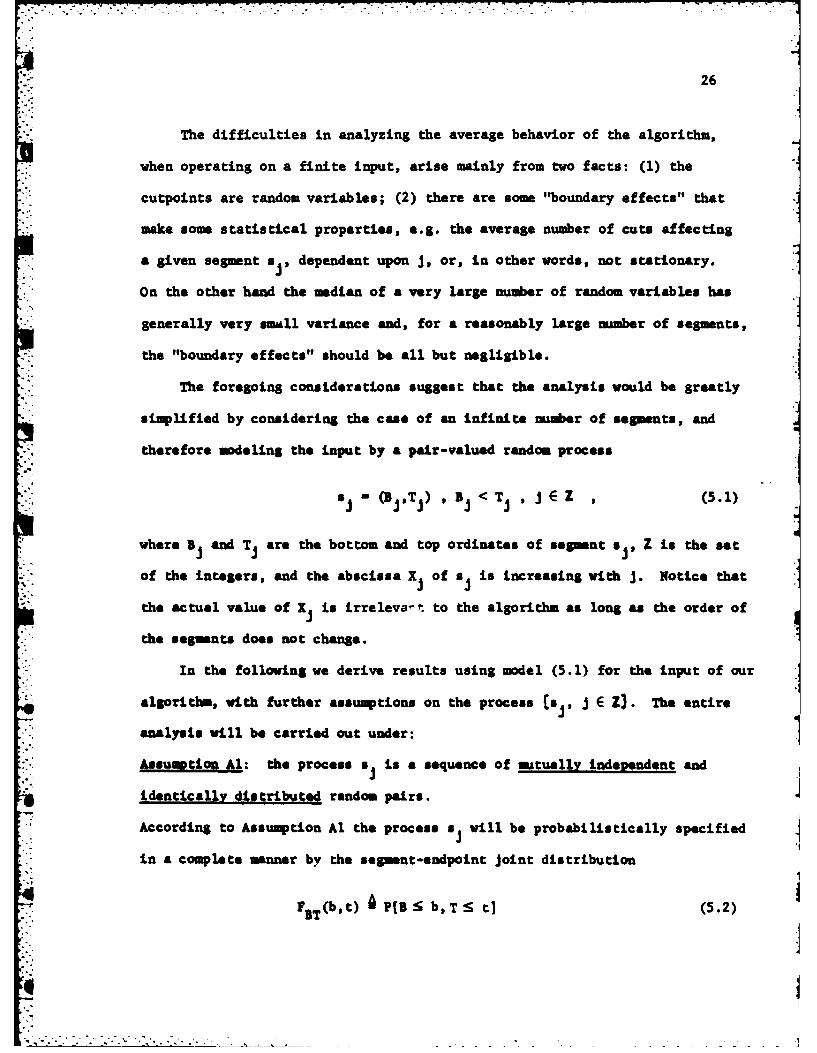
The foregoing considerations suggest that the analysis would be greatly

simplified by considering the case of an infinite number of segments, and

therefore modeling the input by a pair-valued random process

S(5.T~ ~I < T ,j EZ ,(5.1)

where Bi and T are the bottom and top ordinates of segment s, Z is the set

of the integers, and the abscissa X of s is increasing with J. Notice that

the actual value of X is irreleva-t to the algorithm as long as the order of

the segments does not change.

In the following we derive results using model (5.1) for the input of our

algoritb, with further assumptions on the process (5j, J E Z3. The entire

analysis will be carried out under:

Aseumotion Al: the process s is a sequence of mutually independent and

identically distributed random pairs.

According to Assumption Al the process sj will be probabilistLcally specified

in a complete manner by the segment-endpoint joint distribution

F (b,t) P[B: b,T g tI (5.2)BT

27

which is, by hypothesis, independent of J. Here and in the sequel, we follow

" !the convention of denoting a random variable by a capital letter and the

values it assumes by the corresponding lower case letter.

Generators. While the bottom B and the top T are a natural description of

a vertical segment, for our purposes it is convenient to consider the

segment endpoints U and V to be an unordered pair from which B and T can

be recovered as

B - min(U,V], (5.3a)

T = maxCU,V] . (5.3b)

We call U and V generators of the segment and we describe them probabilistically

by the joint distribution

F w(u'v) <-U SU, v S_ v] .(5.4)

There are several advantages in working with generators. One is that

generators can be assumed symmetrically distributed, i.e. FUV(u,v) - Fuv(VsU),

and therefore identically distributed, i.e. Fu(u) - Fv(u). Here

Fu(u) A P[U 5 ul and Fv(v) - P[V v] are the marginal distribution functions

of U and V. Horeover, for the generators we may assume independence together

with identical distribution, while this is not possible for B and T, since

B ! T.

It is also important to notice that there is no loss of generality in

.- -considering generators. In fact, given B and T we can always construct some

generators U and V with the desired properties of symmetry by letting

28

U - QB + (1-Q)T, (5.5a)

V - (I -Q)B + QT, (5.5b)

when Q E to,.] is a random variable, independent of B and T, with

P[Q - O] - P[Q - 11 It is easy to show that for such U and V the

joint distribution is

FwV(uv) - h,(FS(uv) + FBT(v'u)) , (5.6)

and therefore Fuv(u,v) - Fw(Vu).

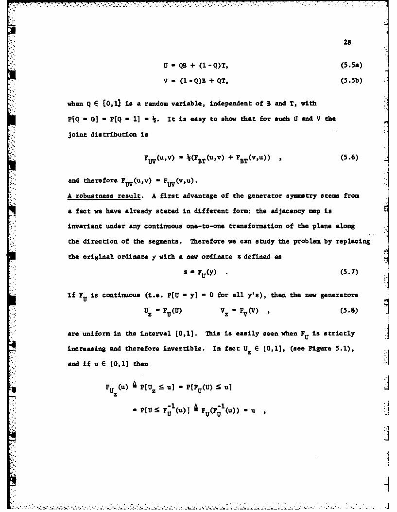
A robustness result. A first advantage of the generator symmetry stems from

a fact we have already stated in different form: the adjacency map is

invariant under any continuous one-to-one transformation of the plane along

the direction of the segments. Therefore we can study the problem by replacing

the original ordinate y with a new ordinate z defined as

z - Fu(Y) . (5.7) :

If FU is continuous (i.e. P[U - y] - 0 for all y's), then the new generators

Uz - (U) Vz -Fv(V) (5.8)

are uniform in the interval (0,1]. This is easily seen when FU is strictly

increasing and therefore invertible. In fact U z E (0,1], (see Figure 5.1),

and if u E [0,1] then

Fu (u) U Pu z < u] - PEFu(U) S u]Uz

-P(US F-(u)] F (F; (u)) -u

i-..

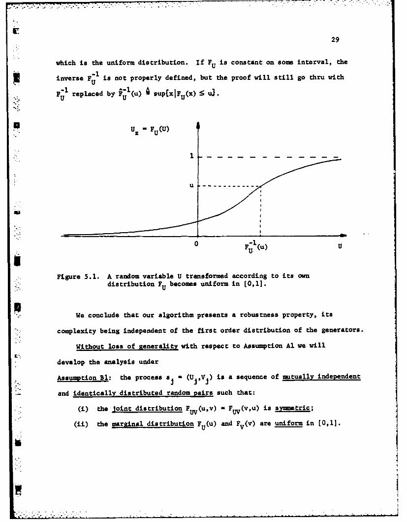
29

which is the uniform distribution. If Fu is constant on some interval, the

inverse F-1 is not properly defined, but the proof will still go thru with

, replaced by -l(u) A sup(xtFu(X) 5 Ul.

* U.. - u(U)

u o-

0 F (u) U

UU

Figure 5.1. A random variable U transformed according to its owndistribution Fu becomes uniform in [0,1].

IU

We conclude that our algorithm presents a robustness property, its

complexity being independent of the first order distribution of the generators.

Without loss of generality with respect to Assumption Al we will

develop the analysis under

Assumption B1: the process sj - (Uj,Vj) is a sequence of mutually independent

-- and identically distributed random pairs such that:

(i) the Joint distribution FUV(u,v) - Fuv(v,u) is synmetric;

(ii) the marginal distribution F.(u) and Fv(v) are uniform in [0,1].

ki °

30

5.2. The Goals of the Analysis: Space and Time

The first quantity we want to analyze is the number S of nodes in the

. search tree. For the case of n segments, if the algorithm cuts segment s

by means of c medians, we have

nS 3n+ E c€ • (5.9)

In fact there are 2n V-nodes, one for each endpoint, and (c+1) O-nodes for

a segment cut c times. Denoting by E the expectation operator on random

variables, our goal is to compute E(cj] to get

'- n

E[SI- 3n + E E(cjI . (5.10)

in our model where n is *, Eqs. (5.9) and (5.10) have no sense, but we can

stIll compute E[cj]. If this quantity turns out to be finite we can say

that our algorithm has asymptotically linear storage, and we can estimate the

storage, at least for large values of n, by the formula

E[S]- (3 + E[c])n . (5.11)

Here and in the following we drop the subscript j in segment s and related

quantities such as cj, since their statistical properties are independent

of j due to the stationarity of the input process.

As far as the time analysis is concerned, we have seen that the

worst-case performance is O(nlogn) both for presorting and SEARCHTMEE.

However the work per endpoint in each recursive call of SEARCHTREE that

processes that point is bounded by a constant. Therefore if we can prove

that the average number of calls in which a point is processed is constant

we can conclude that SEARCHTREE runs in expected linear time.

31

5.3. Principal Slabs and Principal Medians

In order to analyze the algorithm we take a look at the way it works

- and introduce a suitable terminology to describe it. A slab whose y-interval

is of the kind [O,y] or [y,l] is called external. The probability that there

*is a spanning segment in an external slab is zero. Hence the algorithm will

process an external slab by cutting it at the median, which, with probatLlity 1,

is the arithmetic mean of bottom and top of the slab. For example the first

cut will be at y - 4, and will generate the slabs [0,4] and [,l]; slab

[0,4] will be cut at y - 3 and so on. Cuts of external slabs will generate

the following family of medians we call principal medians:

VZ Amkjk Z(5.12)

where m mk A 2 k l for k < 0, mk A 1 -2

"(k+ ') for k > 0. Correspondingly

the following principal slabs are formed:

(slab (u,,,m 4] , k:5 1,

slab(k) - (5.13)

, slab[mk_,,mk] k k 1

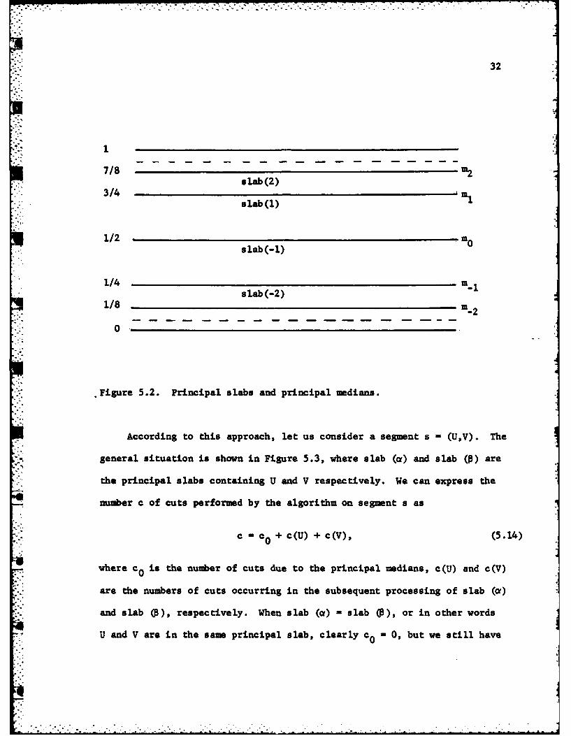
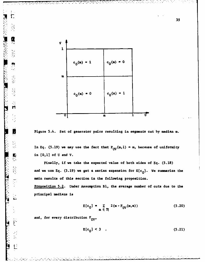
The principal slabs are shown in Figure 5.2.

It is convenient to analyze the procedure SEARCHTREE separating the stage

in which the principal medians are formed from the subsequent processing of the

" interiors of the principal slabs. One reason for this approach is that

(depending on the distribution F ) the principal slabs will generally be

partitioned into rectangles by spanning segments. Medians in rectangles have

1 only a local effect and need to be analyzed differently.

°

32

1

7/8 m23slab(2)""3/4 "M,

slab (1)

1/2 . 0slab(-l)

1/4 m-1slab(-2)

1/8 . 2

0*

Figure 5.2. Principal slabs and principal medians.

According to this approach, let us consider a segment s - (U,V). The

general situation is shown in Figure 5.3, where slab (a) and slab ( ) are

the principal slabs containing U and V respectively. We can express the

number c of cuts performed by the algorithm on segment s as

c = co + C(U) + c(V), (5.14)

where co is the number of cuts due to the principal medians, c(U) and c(V)

are the numbers of cuts occurring in the subsequent processing of slab (Cf)

and slab Q3), respectively. When slab (d) = slab (3), or in other words

U and V are in the same principal slab, clearly c0 -0, but we still have

7 -7 77,

it 33

c(U) cuts IU slab(q)

c cuts0

c(V) cuts V slab)03

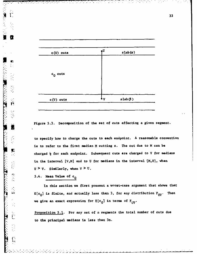
Figure 5.3. Decomposition of the set of cuts affecting a given segment.

to specify how to charge the cuts to each endpoint. A reasonable convention

is to refer to the first median M cutting s. The cut due to M can be

charged k for each endpoint. Subsequent cuts are charged to V for medians

in the interval [V,MI and to U for medians in the interval IM,U], when

U > V. Similarly, when V > U.

5.4. Mean Value of co

In this section we first present a worst-case argument that shows that

Lo E[cO] is finite, and actually less than 3, for any distribution FUV. Then

we give an exact expression for Elc OI in terms of FV.

Proposition 5.1. For any set of n segments the total number of cuts due

to the principal medians is less than 3n.

34

Proof. The claim follows by considering that, if on one side of median m

there are q points, median m cuts at most q segments. Therefore mn0 cuts

at most n segments, M.1 and m1 cut at most n/2 segments each, and so on.

Of cours- only a finite set 4* of principal medians is to be considered.

Thus

n nZ = Eo. (m)-,<n+2( n+ n+ ..) 3n (5.15)j-1l Jm mE*-

where coj(m) - 1 if m cuts segment sj, and coj(m) - 0 otherwise.

From (5.15) we get

in :n £l E[€0]<_ 3 ,(5.16)

which is the stationary model, where n - and E[co]- E[co], becomes

E[coI < 3 . (5.17)

To compute E[co] exactly we write co in terms of co(m) as

C0 c c 0 (m) . (5.18)m, E 74

Since cO(m) E C0,11, we have

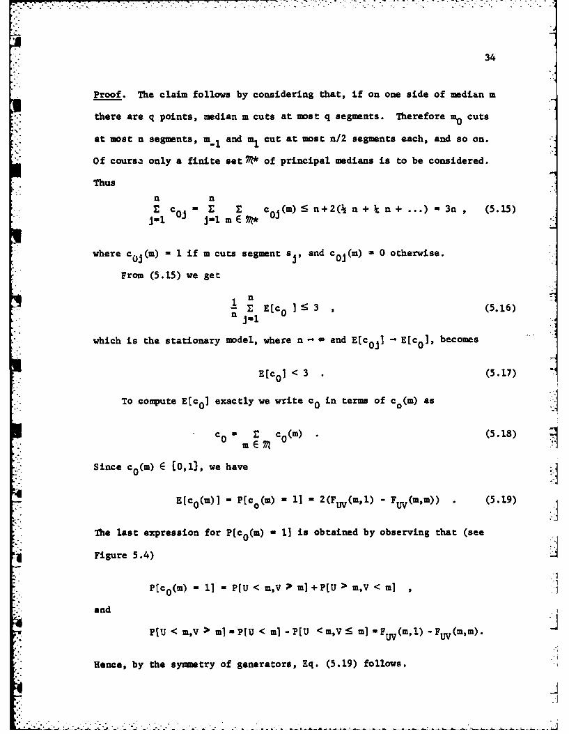
E(co(m)] - P[co(m) - 11 - 2 (FUV(m,l) - FUV(m,m)) . (5.19)

The last expression for P[co(m) - 11 is obtained by observing that (see

Figure 5.4)

P[co(m) -11-P[U< m,VmI+P[U> Mr,V< m]

and

PJU < m,V > ml-PJU < m] -P[U < m,V<S m] Fu (m, 1) =F r(r,m).

Hence, by the symnetry of generators, Eq. (5.19) follows.

• ;- i' : :. _ .: ..,- :; _- ._. .: ; --: 2 i. _. ... -.. i -. .. .... _ -. . .. .' .. ." ... . _I .

"-.' 35

V

COW CO W

I C0 (m) 1 C()

• •:. :•:Co(m) - 0 co(m) - 1

Figure 5.4. Set of generator pairs resulting in segments cut by median m.

In Eq. (5.19) we may use the fact that Fu(m,1) - m, because of uniformity

in [0,1] of U and

V.

Finally, if we take the expected value of both sides of Eq. (5.18)

and we use Eq. (5.19) we get a series expansion for E[c0 ]. We summarize the

main results of this section in the following proposition.

Proposition 5.2. Under Assumption Bl, the average number of cuts due to the

principal medians is

E(c - E 2(m-FtV (m,m)) (5.20)

S . and, for every distribution F

Ec .] < 3 . (5.21)i0t2

36

Incidentally, we note that bound (5.21), derived here as a consequence

of Proposition 1, can be obtained directly from Eq. (5.20). For this purpose

in Eq. (5.20) the range of suuation 7, defined in Eq. (5.12), can be split

in sets tmkjkk 01 and tmkk > 01. The sum is then upper bounded using the

fact that in the first set mk - FUW(mk,mk) - mk - 2 k , and, in the second set,

mk - FUV(mk,mk) -5 (1 - n.k) - 2 " ( k+l). The result (5.21) then follows by

the sum of two geometric series.

5.5. Analysis of Rectangles in Principal Slabs

We still have to analyze the contribution of c(U) and c(V) to c, in

Eq. (5.14). For this task we need to consider the work done by the algorithm

when processing the interiors of the principal slabs. In general a given

generator, say U, will be contained in a rectangle R formed by the boundary

medians of a principal slab together with two spanning segments. Since the

algorithm processes the rectangles independently of each other, c(U) is

determined only by the contents of R. Intuition suggests that, on the average,

c(U) increases with the total number W of points in R. This we shall now

analyze.

* Analysis of segments. We begin by studying the relative position of a

segment and a generic slab [m, ']. We define the set of segments that

respectively: (i) span the slab, (ii) have one endpoint in the slab,

(iii) have two endpoints in the slab, or (iv) are outside the slab. More

formally

, I < m, m' < T (5.22a)

CsKB < m < T < m' or m < B < m' < T] (5.22b)

L1

37

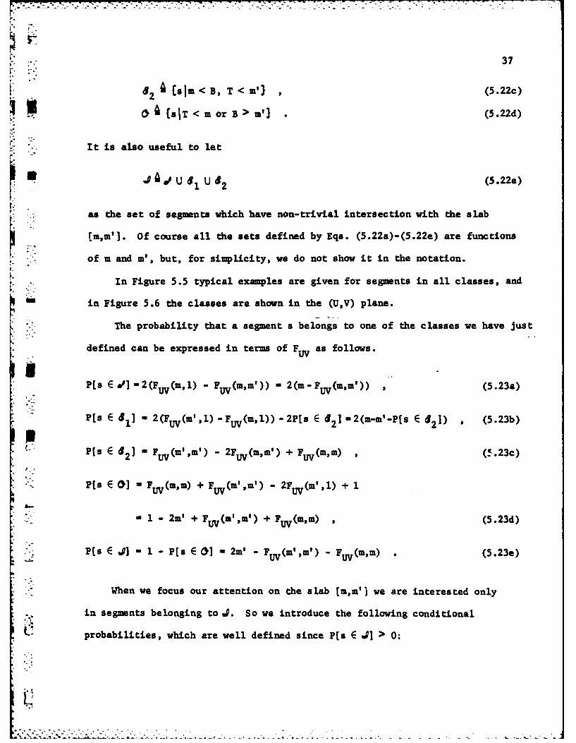
2 t sIm < B, T < m') , (5.22c)

sIT < m orB B ' . (5.22d)

It is also useful to let

Sd U a U 42 (5.22e)

. ;as the set of segments which have non-trivial intersection with the slab

[m,m']. Of course all the sets defined by Eqs. (5.22a)-(5.22e) are functions

of m and m', but, for simplicity, we do not show it in the notation.

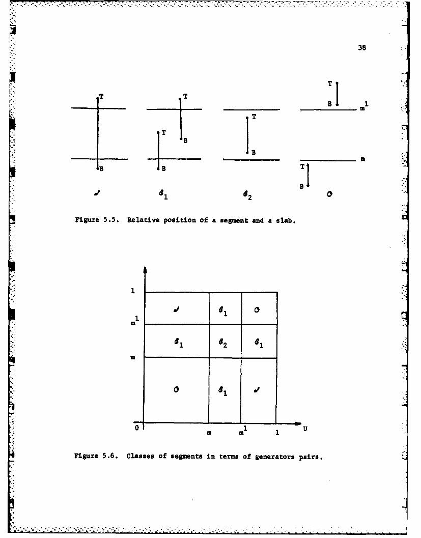
In Figure 5.5 typical examples are given for segments in all classes, and

-in Figure 5.6 the classes are shown in the (U,V) plane.

The probability that a segment a belongs to one of the classes we have just

defined can be expressed in terms of FUV as follows.

P[s E W] 2(Fuv(m,l)- Fuv(m,m))- 2(m -FUV(mm')), (5.23a)

P[s E 4 1 - 2 (Fuv(m',l) -Fuv(m,l)) -2P[s E 42] 2(m-m'-P[s E 2 ) ) (5.23b)

pP[s E 4 21 - FUV(m',m') - 2FUV(m,m') + FUV(m,m) , (!.23c)

- P[s E 01 FUV(m,m) + Fuv(m',m') - 2FUV(m',l) + 1

1 1 - 2m' + F(v(m',m') + FUV(m,m) , (5.23d)

P[s E ,01 = 1 - P[s E 0] = 2,' - FUV(m',m') - Fuv(m,m) . (5.23e)

When we focus our attention on the slab [m,m'] we are interested only

in segments belonging to J. So we introduce the following conditional

probabilities, which are well defined since P(s E J] > 0:

o

38

TI

IT T- - ___ ____ __ ____ ___ __B

TT

B B B

a, ~1B

Figure 5.5. Relative position of a segment and a slab.

1 12

*0 0

0 1

Figure 5.6. Classes of segments in terms of generators pairs.

-..- 7 .

U39

Po PIs E **Is E J1 Prs E ]/P[s E A (5.24a)

P1 PIs E &,Is E J1= P[S E 81]/Pts E A] (5.24b)

p2 A Fs E ,15 E .I1 - Ps 6 52 ]/P~s 6 J] . (5.24c)

To guarantee the existence (with probability 1) of rectangles in the

principal slabs, we introduce the following assumption, that is satisfied

by most reasonable distributions.

Assumption A2: the distribution FUV is such that probability p0 is nonzero

for all the principal slabs.

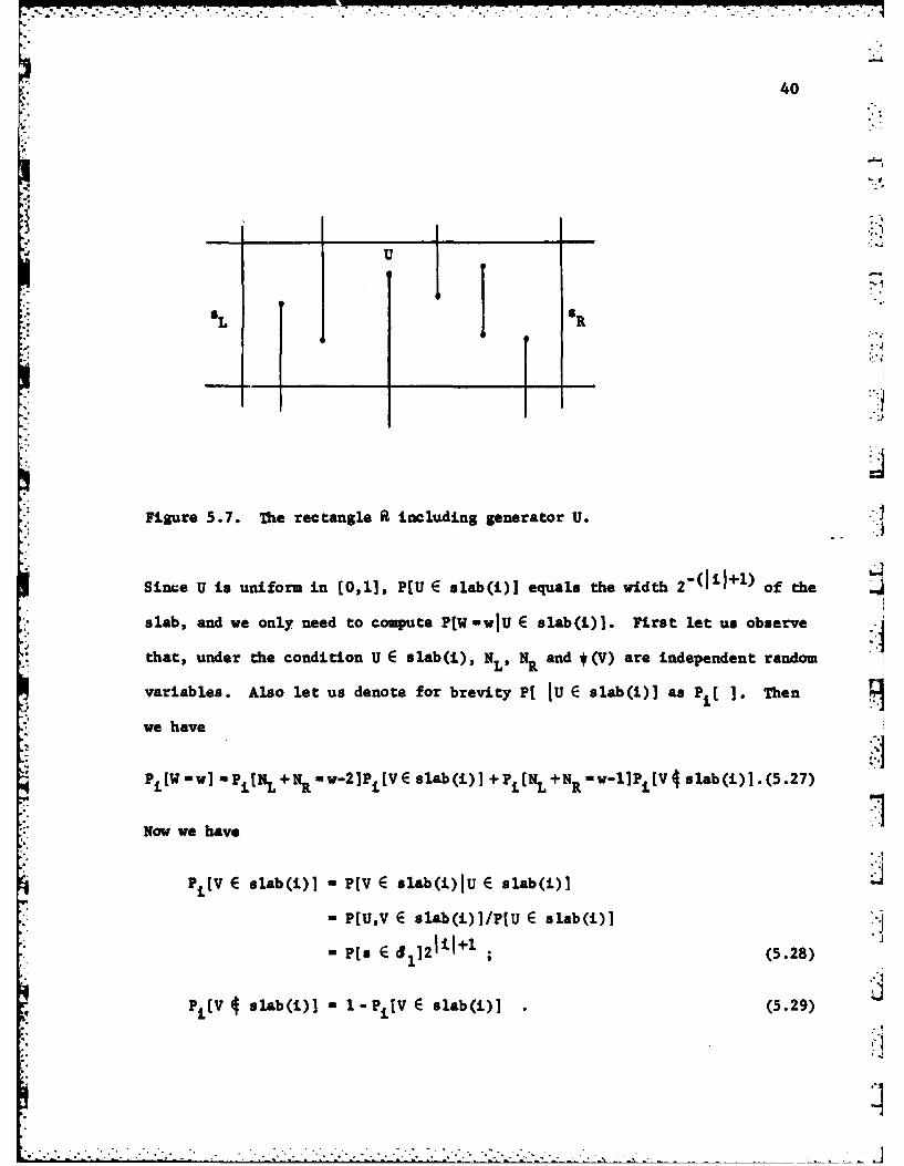
Analysis of rectangles. Let us now consider a generator of s, say U E slab(i).

Let sL and 9 the left and the right segments closest to U, among those

which span slab(i), and call R the rectangle closed by these two segments.

The number W of segment endpoints in node R can be written as

W N "L +N + 1+ (V) , (5.25)

where NL is the number of points in R to the left of U, NR is the number of

those to the right, the third term, 1, accounts for U itself, and #(V) is 1

if V - the other generator of s - is also in slab(i) and 0 otherwise. An

example is given in Figure 5.7, where V slab(i) so that 4(V) - 0,

NL: =2, N - 4, and W - 2+4+1+0 - 7.

Now we want to find the probability mass function (p.m.f.) of W. It is

useful to partition the sample space into regions where U belongs to a given

slab. The theorem on total probability for this partition yields

PEW -w] - SPEW -wIU E slab(i)]P(U E slab(i) . (5.26)

. A

40

U

J -

iL R

Since U is uniform in 10,11, P[U E slab(i)I equals the width 2- i~)of the

slab, and we only need to compute P[W -wJU E slab(i)]. First let us observeI

that, under the condition U E slab(i), NL , N R and 4(V) are independent random

variables. Also let us denote for brevity P[ IU E slab(i)J as Pil 1. Iten

we have

*P:L[W w] - Pi[NL +NR -w-2]Pi(V Eslab(i)1 + Pi[NL+N R mw-]P±[V slab (1)](5.27)

Now we have

PiEV E slab(i)] - P[V E slab(i)IU E slab(i)]I

- P[U,V E slab(i)]/P[U E slab(i)]J

- Pr, E 4 12 1'1+1 (5.28)1.1

I s a and e ol y nee 1 -o op u e U E slab(]. (5r.29

b41

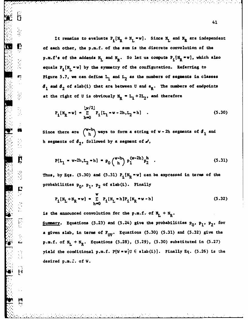
It remains to evaluate PI[NR + NL -w]. Since NL and NR are independent

of each other, the p.m.f. of the sum is the discrete convolution of the

p.m.f's of the addends NL and NR . So let us compute Pi[NR-W], which also

equals Pi[. -w] by the symmtry of the configuration. Referring to

Figure 5.7, we can define L and L2 as the numbers of segments in classes

a and 2 of slab(i) that are between U and a The numbers of endpoints

*. at the right of U is obviously NR = LI+2L2 , and therefore

L/2L

.. iN R.- w] E Pi[L -w-2hL 2 - h ] . (5.30)h-O

Since there are (h) ways to form a string of v - 2h segments of 4and

h segments of 82, followed by a segment of W,

PtL 1 - w-2hL 2 h] Po (h (w-2h) h (5.31)

Thus, by Eqs. (5.30) and (5.31) P [NR-w] can be expressed in terms of the

probabilities pO, pl, P2 of slab(i). Finally

wPi[NL+NR-w - E Pi[NL-h]Pi[NR-w-hl (5.32)

h-0

is the announced convolution for the p.m.f. of NL + N .

- Sumary. Equations (5.23) and (5.24) give the probabilities pO, pl, P2 ' for

a given slab, in terms of F,,. Equations (5.30) (5.31) and (5.32) give the

p.m.f. of NL + NR. Equations (5.28), (5.29), (5.30) substituted in (5.27)

yield the conditional p.m.f. P(W-wJU E slab(i)]. Finally Eq. (5.26) is the

desired p.m.Z. of W.

17-

-

42

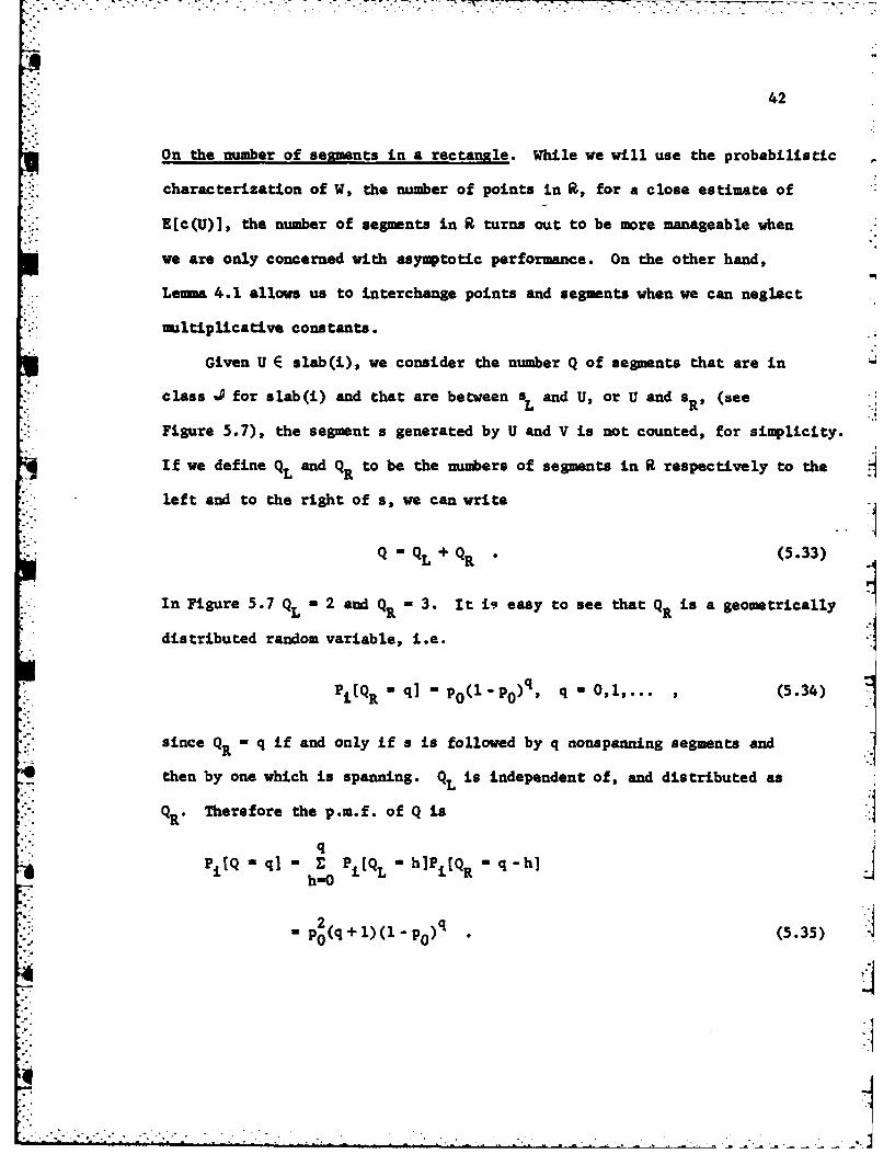
On the nmmber of seaments in a rectangle. While we will use the probabilistic

characterization of W, the number of points in R, for a close estimate of

E[c(U)], the number of segments in R turns out to be more manageable when

we are only concerned with asymptotic performance. On the other hand,

Lemma 4.1 allows us to interchange points and segments when we can neglect

.m ltiplicative constants.

Given U E slab(i), we consider the number Q of segments that are in

class J for slab(i) and that are between 8 and U, or U and sR, (see

. Figure 5.7), the segment s generated by U and V is not counted, for simplicity.

If we define QL and Q to be the numbers of segments in R respectively to the

"* left and to the right of s, we can write

Q =QL + QR "(5.33)

In Figure 5.7 QL - 2 and QR - 3. It iq easy to see that Q is a geometrically

distributed random variable, i.e.

•Pi[Q R q] =po(l -po)q , q =0,1,... ,(5.34)

since QR q if and only if s is followed by q nonspanning segments and

then by one which is spanning. QL is independent of, and distributed as

Q Therefore the p.m.f. of Q is

qP [Q q] - P Pi1QL - h]Pi[QR - q-h]

" p0(q+ 1)(1 -) . (5.35)

0I

. .° . I.

43

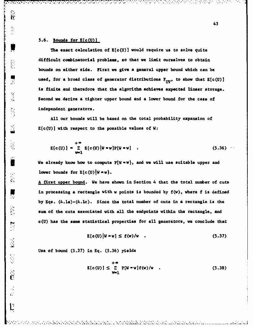
5.6. Bounds for E[c(U)]

The exact calculation of E[c(U)] would require us to solve quite

difficult combinatorial problem, so that we limit ourselves to obtain

bounds on either side. First we give a general upper bound which can be

used, for a broad class of generator distributions F , to show that E[c(U)]

is finite and therefore that the algorithm achieves expected linear storage.

Second we derive a tighter upper bound and a lower bound for the case of

independent generators.

All our bounds will be based on the total probability expansion of

E[c(U)] with respect to the possible values of W:

E(c(U)]- E E[c(U)IW-w]P[W-w] . (5.36)w-1

We already know how to compute PEW -vi, and we will use suitable upper and

lower bounds for E[c(U)IW-w].

A first upper bound. We have shown in Section 4 that the total number of cuts

in processing a rectangle with w points is bounded by f(w), where f is defined

by Eqs. (4.1a)-(4.1c). Since the total number of cuts in a rectangle is the

C. sum of the cuts associated with all the endpoints within the rectangle, and

_c (U) has the same statistical properties for all generators, we conclude that

E[c(U)IW-w] _< f(w)/w . (5.37)

Use of bound (5.37) in Eq. (5.36) yields

E[c(U)j < E PEW-wlf(w)/w (5.38)

12*...................

.-.

44

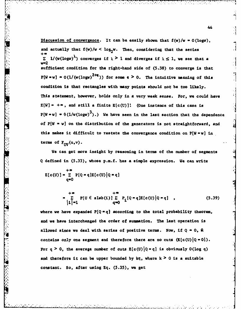
Discussion of convergence. It can be easily shown that f(w)/w s O(logw),

and actually that f(w)/w < log2w. Then, considering that the series

E l/(w(logw) ) converges if ) > 1 and diverges if X : 1, we see that aw-2sufficient condition for the right-hand side of (5.38) to converge is that

PEW-w] -O(1/(w(logw)2)) for somese > 0. The intuitive meaning of this

condition is that rectangles with many points should not be too likely.

This statement, however, holds only in a very weak sense. For, we could have

E[W] = +m, and still a finite E[c(U)I! (One instance of this case is

P[W-w] - (/w(logw) We have seen in the last section that the dependence

of P[W - w] on the distribution of the generators is not straightforward, and

this makes it difficult to restate the convergence condition on PEW -w] in

terms of F UV(u,v).

We can get more insight by reasoning in terms of the number of segments

Q defined in (5.33), whose p.m.f. has a simple expression. We can write

E[c(U)l- E P(Q-qiE[c(U)IQ q]q=O

E = P(UE slab(i)] E PI[Q-q]E[c(U)IQ-q] , (5.39)"iI-1 q0

where we have expanded P(Q -qJ according to the total probability theorem,

and we have interchanged the order of sumation. The last operation is

allowed since we deal with series of positive terms. Now, if Q - 0, R

contains only one segment and therefore there are no cuts (E[c(U)Q-0).

For q > 0, the average number of cuts E[c(U)IQ-q] is obviously O(log q)

and therefore it can be upper bounded by kq, where k• 0 is a suitable

constant. So, after using Eq. (5.35), we get

.~~~~ .. .

45

2 2 +q

E P1[Q-q]E[c(U)IQ-q] 5 k p0£ E (q+1)q(l-P01 ) (5.40)q-0 q-l

The last series can be sumed in closed form yielding

+0 2 2 2k (5.41)Eino Pi[Q-q]E[c(U)IQ-ql :5 P0 P~P 3q-0o POL o

Note that we have added the subscript i to pO to stress its dependence on

the slab. Substitution of bound (5.41) in Eq. (5.39) gives

Ec(U)] 5 2k E 2-(1i1+l) _ +

+0 -1 +0 2-ik E- + k . (5.42)"£'1 POL ini PO(-i)

A sufficient condition for convergence of the last term, and therefore for

finiteness of E(c(U)], is that

P0L > k' 2" i(log 1)1+ • , I 1 (5.43)

for some k' > , and some c > 0, and a similar condition for i!5 1.

Condition (5.43) is not very restrictive at all. It is intuitive that a

lower bound on the probabilities of spanning segments prevents rectangles

with many segments. The lower bound is decreasing with ILI because slabs

with fewer points have less weight in the contribution to the number of cuts.

I.

t ".

46

*Independent generators. To get less crude bounds than the one expressed by

Eq. (5.38), we need to further specify the joint distribution FUV of the

generators. We introduce

Assumption A3 (independence). U and V are statistically independent, with

joint distribution

Fuv(u,v) = Fu(u)Fv(v) = u v, u,v E [0,1] (5.44)

The hypothesis of independence considerably simplifies the analysis.

Here we see another advantage of defining generators; in fact, as already

noted, we could not directly assume independence together with indntical

distribution for the bottom B and the top T of segment s, since B 5 T.

Let R be a rectangle processed by the algorithm in slab [mm'], not

necessarily a principal one. in any case R will be completely below

(m' S k) or completely above (m k 2) the median m0 = . The median M of

the points in R divides P. into two parts: we call internal the one closer to

m =, and external the other one. So the internal part is the one above M

for rectangles below m0, and the ones below M for rectangles above m.

Let z be the endpoints inside R. Without loss of generality

suppose that R is above inm, as shown in Figure 5.8. If z E R is a

generator of segment (zj, i), this segment is cut by median M if and only if

z < M and z M H, or z > m and < M. If we call c(z,14) the number of cuts

due to M and charged to z, we have:

S[(z;M) =11]= 0 z as M (5.45)

{-M z < M

47

external

-C H

internal

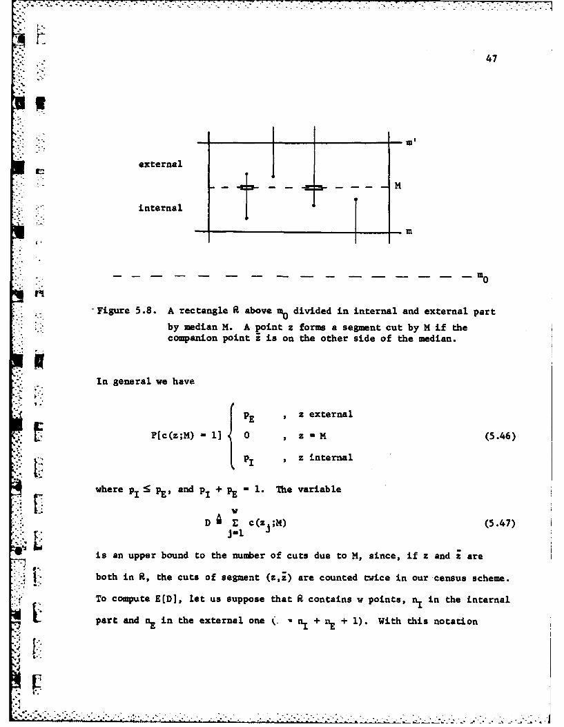
-Fiure5.8 Arectangle above modivided in internal and external part

by median H. A point z forms a segment cut by M if thecompanion point is on the other side of the median.

In general we have { E 9 z external

p1 ~ , internal

where p 1 :5 pE, and p, + -E 1. The variable

is an upper bound to the number of cuts due to M, since, if z and ;are

both in R, the cuts of segment (z,i) are counted twdice in our census scheme.

To compute E(D], let us suppose that P. contains w points, n., in the internal

part and nE in the external one i r.' n + nE + 1). With this notation

-, 48

E[D] E[c(z ;M)]

- P[c(z ;4) -1] n.p + nEP (5.48)

If we choose the median M4 much that n1, - n.- (w-l)/2 when w is odd, and

n.-k +1 -w/2 when w is even, we have that

{(w-l)/2 odE(D] -(5.49)

w2- 1 + p1 w even

and in general, being P, < 1

w/2 1:15- E(D] <(w-l)/2 .(5.50)

The number of cuts in a given rectangle R equals the number of cuts due to

the median M plus the number of cuts occurring in the two regions obtained

by cutting R with M. In the worst case such regions will consist of only

one rectangle, while in general spanning segments will form several

rectangles in each region. Based on these considerations we can

recursively define an upper bound g(w) for the average number of cuts

occurring in a rectangle with w points.

g(0)in0, g(l) 0O (5 .51a)

g(w) -(w-l)/2 + g(n 1 ) + g(oE) ,(5.51b)

where, as we have said, n1, - L(w-l) /2J, I E - r(w-l)/21 .Using the bound

g(w)/w for E[c(U)jW -w] in Eq. (5.36) we get

7-.. . . . .. .- - ., ..1 -

... . , - . -7

Ia 49

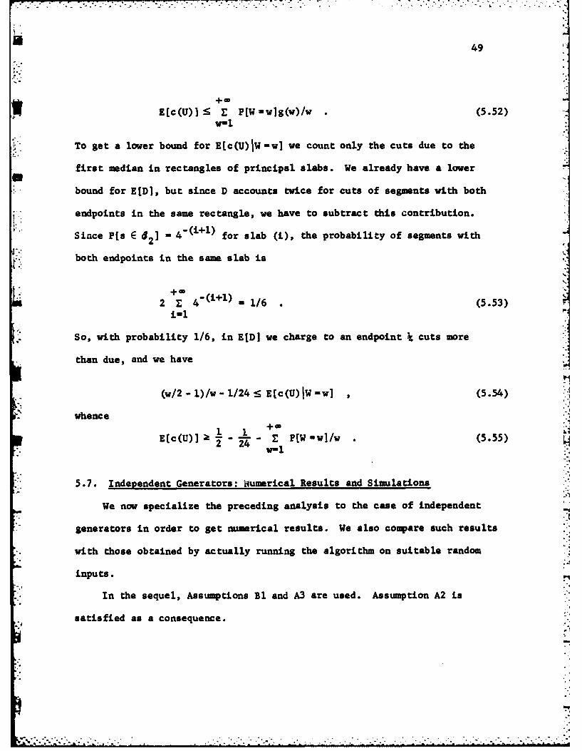
E[c(U)J -< E P[W--wlg(w)/w . (5.52)v-1

To get a lower bound for Elc(U)IW -w] we count only the cuts due to the

first median in rectangles of principal slabs. We already have a lower

bound for E[D], but since D accounts twice for cuts of segments with both

endpoints in the same rectangle, we have to subtract this contribution.

Since P[s E 2 = 4-(i+l) for slab (i), the probability of segments with

21.

. both endpoints in the same slab is

2 4-(+) - 1/6 . (5.53)i-l

So, with probability 1/6, in E[D] we charge to an endpoint Cuts more

than due, and we have

(w/2 -1)/w - 1/24 ! E[c(U)(W-w] (5.54)

whence

E c(U)] - - E P[W Mw]/w (5.55)V-.1w, l

5.7. Independent Generators: Numerical Results and Simulations

We now specialize the preceding analysis to the case of independent

generators in order to get numerical results. We also compare such results

• .with those obtained by actually running the algorithm on suitable randomm..

inputs.

In the sequel, Assumptions Bl and A3 are used. Assumption A2 is

satisfied as a consequence.

* -1!

-,o . O . . .-. . o o . - . . - .. . .

50

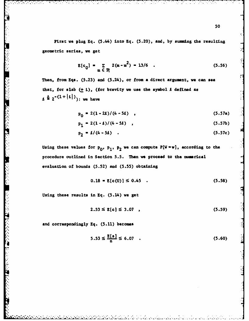
First we plug Eq. (5.44) into Eq. (5.20), and, by suamning the resulting

geometric series, we get

E[c0 E 2m- ) -13/6 .(5.56)

Then, from Eqs. (5.23) and (5.24), or from a direct argument, we can see

that, for slab (+ i), (for brevity we use the symbol A defined as

£ 2-(1+1Ii1)): we have

PO 2l -2A)/4 -5A)(5.57a)

p1 -2(l-A)/(4-5A) ,(5.57b)

P2 A/4-5A)(5.57c)

Using these values for po, pl, P2 We can compute P[W -w], according to the

procedure outlined in Section 5.5. Then we proceed to the nmrical

evaluation of bounds (5.52) and (5.55) obtaining

0.18 -E~c(U)1 5 0.45 .(5.58)

Using these results in Eq. (5.14) we get

2.53:5 E~c] 5 3.07 ,(5.59)

and correspondingly Eq. (5.11) becomes

n

51

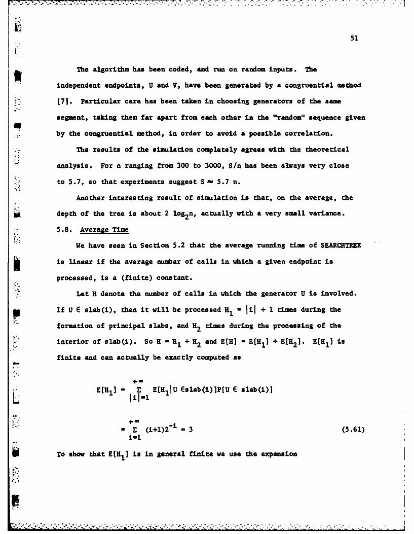
The algorithm has been coded, and run on random inputs. The

independent endpoints, U and V, have been generated by a congruential method

[7]. Particular care has been taken in choosing generators of the same

segment, taking them far apart from each other in the "random" sequence givenS

by the congruential method, in order to avoid a possible correlation.

The results of the simalation completely agrees with the theoretical

analysis. For n ranging from 300 to 3000, S/n has been always very close

to 5.7, so that experiments suggest S a 5.7 n.

Another interesting result of siulation is that, on the average, the

depth of the tree is about 2 log2n, actually with a very small variance.

5.8. Average Time

We have seen in Section 5.2 that the average running time of SEARCUTREE

is linear if the average number of calls in which a given endpoint is

processed, is a (finite) constant.

Let H denote the number of calls in which the generator U is involved.

If U E slab(i), then it will be processed H1 - Il + I times during the

formation of principal slabs, and H2 times during the processing of theinterior of slab(i). So H - l + H2 and E[H] - E[H1 1 + E[H2 ]. E[H1 1 is

finite and can actually be exactly computed as

a-g.

EHE E[lU Eslab(i)]P(U E slab(i)]

- (i+l)2 -3 (5.61)t is

~To show that E[H1 ] is in general finite we use the expansion

.;i,'..,., ., ,,, ... -. .,,'.'-,9 -C..... . . . . . . . . . . . :..• , ........ .. ,.... ..... .,.... .,._ •. .. ,.. ,.. .;...._.,....

52

.

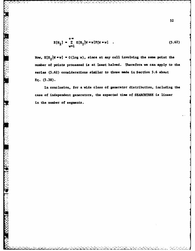
E[H E E= E(U2jWiniPEWiw] • (5.62)f12

Now, E H2I 1W ] = O(log w), since at any call involving the same point the

number of points processed is at least halved. Therefore we can apply to the

series (5.62) considerations similar to those made in Section 5.6 about

Eq. (5.38).

In conclusion, for a wide class of generator distribution, including the

case of independent generators, the expected time of SEARCHTREE is linear

in the number of segments.

;2

53

6. CONCLUSIONS

In this thesis we have defined and analyzed a new algorithm for the

adjacency map, using a technique that can be easily extended to solve the

point location problem in a planar subdivision induced by an embedded

straight-line planar graph.

An advantage of this technique lies in the simplicity of the basic

L idea: the extension of binary search to planar structures. However, dealing

t with two dimensions requires some care in the implementation of the binary

search to keep both the storage and the search time bounded.

From a practical point of view, our algorithm is quite attractive,

since it builds in time O(nlogn) a data structure that can be stored in

space O(nlogn) and searched in time O(logn). Moreover all the constants

involved are small.

Theoretically though, we know that O(n) space is achievable, and

[ therefore the algorithm is not asymptotically optimal in the worst case.

However, while it is possible to find cases in which S (n) - e (nlogn), (the

reader may try with the set Isj - (-J,J)Ij-l,...,n, such cases require

a strong correlation in the position of all the segments. This suggests

that if the segments are random, for instance independent of each other,

the expected value of S(n) should be linear in n.

The analysis developed in Section 5 confirm the foregoing conjecture

and also allows us to estimate the constant k in E[S(n)] - kn, when the

statistical description of the segments is given. In the case of segments

with independent endpoints, we have seen that kaw 6. Comparing this

result with the lower bound discussed in Section 4, that implies k 2 3,

we may conclude that the storage performance of the algorithm is quite good.

54

The preprocessing time is also satisfactory, since, after presorting

the procedure SEARCHTREE runs in average linear time. Finally the search

time is already good (< 3 logn + 7) in the worst case, and siulation

suggests it is slightly better (" 2 logn) on the average.

Beyond the details of the analysis we may like to capture, on an intuitive !

basis, the essential features of the algorithm that make its average time and

space be linear. We can see the action developing as follows. First the

region to be searched is partitioned in O(logn) strips of plane, the

principal slabs in the infinite model, and a point is located in a slab.

Then the search proceeds in the interior of the slab. A segment must be

represented in the search structure of each of the slabs that intersects,

but this can be done at the expense of a small amount of extra storage, since _

on the average a segment intersects less than 4 slabs. Each principal slab

is in turn partitioned in rectangles by the spanning segments. Comparison

against spanning segments allows point location in a rectangle. At this

point we only need a search structure for each rectangle, since different

rectangles do not interfere with each other. The size of such structures

depends on the number of points in the rectangle. The key point is now that

.when the size n of the problem increases, the number of rectangles increases

proportionally, but the distribution of the size of the rectnagles does not

change. Therefore the average time to build, and the average space to

store, the related search-tree are constant. Thus globally, the average

complexity is linear. The constant of proportionality is of course related

to the distribution of the rectangle size, and this in turn to the frequency

of spanning segments. When the endpoints are independent there are many

,.. spanning segments, and this accounts for the fact that the constants are

small in this case.

I'2' " " " " " '" * :' " " " ' ' ' ' : ' " ' ' " " " , "-. ", . .. ,_ "

55

As we have seen, the probabilistic analysis of the adjacency map has

P given considerable insight on the main features of the point-location

technique used. The next step should be to extend the analysis to the

-2 general case of point location in planar graphs. If, as we conjecture,

the complexity of the algorithm is the sa in the general case, the

proposed technique can be considered a basic tool in computational geometry.

ni,'

[ C.

! .-.

56

REFERENCES

1. W. Lipski and F. P. Preparata, "Segments, rectangles, contours,"J. Algorithms 2, (1981) pp. 63-76.

2. D. T. Lee and F. P. Preparata, "Location of a point in a planarsubdivision and its applications," SIAM J. Comput. 6, No. 3 (1977)pp. 594-606.

3. F. P. Preparata, "A new approach to planar point location," SIAM J.Comput., No. 3 (1981) pp. 473-482.

4. R. J. Lipton and R. E. Tarjan, "Application of a planar separatortheorem," Proc. of the 18th Syup. on Found. of Coup. Sci.,Providence, RI, October 1977, pp. 162-170.

5. D. G. Kirkpatrick, '"Optimal search in planar subdivision," Universityof British Columbia, Vancouver, British Columbia, Department ofComputer Science; Manuscript, 1979.

6. E. M. Reingold, J. Nievergelt and N. Deo, Combinatorial Algorithms,Prentice-Hall, Inc., Englewood Cliffs,. NJ, 1977.

7. D. E. Knuth, The Art of Computer Programming, Vol. 2, Addison-Wesley,1969.

,. .

V!

FILMED

3 8 3

DTIC