HAL Id: hal-02399695https://hal.inria.fr/hal-02399695

Submitted on 9 Dec 2019

HAL is a multi-disciplinary open accessarchive for the deposit and dissemination of sci-entific research documents, whether they are pub-lished or not. The documents may come fromteaching and research institutions in France orabroad, or from public or private research centers.

L’archive ouverte pluridisciplinaire HAL, estdestinée au dépôt et à la diffusion de documentsscientifiques de niveau recherche, publiés ou non,émanant des établissements d’enseignement et derecherche français ou étrangers, des laboratoirespublics ou privés.

Asynchronous pi-calculus at Work: The Call-by-NeedStrategy

Davide Sangiorgi

To cite this version:Davide Sangiorgi. Asynchronous pi-calculus at Work: The Call-by-Need Strategy. The Art of Mod-elling Computational Systems: A Journey from Logic and Concurrency to Security and Privacy, Nov2019, Paris, France. pp.33-49, �10.1007/978-3-030-31175-9_3�. �hal-02399695�

This is a post-peer-review, pre-copyedit version of an article published inLecture Notes in Computer Science, vol 11760. The final authenticated versionis available online at: https://doi.org/10.1007/978-3-030-31175-9 3

This version is subjected to Springer Nature terms for reuse that can be found at:

https://www.springer.com/gp/open- access/authors-rights/aam-terms-v1

1

Asynchronous π-calculus at work:the call-by-need strategy

Davide Sangiorgi

Focus Team, University of Bologna and INRIA

Abstract. In a well-known and influential paper [17] Palamidessi hasshown that the expressive power of the Asynchronous π-calculus is strictlyless than that of the full (synchronous) π-calculus. This gap in expres-siveness has a correspondence, however, in sharper semantic propertiesfor the former calculus, notably concerning algebraic laws. This papersubstantiates this, taking, as a case study, the encoding of call-by-needλ-calculus into the π-calculus. We actually adopt the Local Asynchronousπ-calculus, that has even sharper semantic properties. We exploit suchproperties to prove some instances of validity of β-reduction (meaningthat the source and target terms of a β-reduction are mapped onto be-haviourally equivalent processes). Nearly all results would fail in the ordi-nary synchronous π-calculus. We show that however the full β-reductionis not valid. We also consider a refined encoding in which some furtherinstances of β-validity hold. We conclude with a few questions for futurework.

1 Introduction

A lot of effort has been devoted to the comparison of the π-calculus with theλ-calculus, beginning with Milner’s seminar work on functions as processes [14].The attention has gone mostly to call-by-name and call-by-value λ-calculi [19],and the main results concern operational correspondence, validity of β-reduction,characterisation of the equivalence induced on λ-terms by the π-calculus encod-ing [14, 21, 22, 27, 6]. In particular, the call-by-name encoding, for its simplicity,is often presented as the π-calculus representation of functions.

In a call-by-name reduction, the redex contracted is the leftmost one; thereduction occurs regardless of whether the argument of the function is a value(as in call-by-value). As a consequence, if the argument is not a value and willbe used several times, its evaluation will be repeated the same number of times.In implementation of programming languages following call-by-name, this rep-etition of evaluation is avoided: evaluation occurs only once, the first time theterm is used, and the value so obtained is recorded for future uses. This imple-mentation technique is referred to as call-by-need evaluation (or strategy) [28].Thus call-by-need uses explicit environments and β-reduction does not requiresubstituting a term for a variable, as in call-by-name (or call-by-value) — justsubstituting a reference to a term for a variable. In this sense call-by-need iscloser to the π-calculus than call-by-name, as substitutions in the π-calculus

only involve names. Again, the modifications that take us from call-by-name tocall-by-need can be easily represented in a π-calculus encoding [24].

The π-calculus, having a rich and well-developed theory, as well as a remark-able expressiveness, has been advocated as a foundational model for reasoningabout higher-order languages, including equivalence between programs and cor-rectness of compilers and compiler optimisations [25, 26]. Indeed, the π-calculusand related languages have been used, via appropriate encodings, as a targetlanguage of compilers, for a number of experimental programming languages,beginning with Pict [18] and Join [7].

The above raises the question about how, and at which extent, the π-calculusand its current theory can be used to prove the correctness of call-by-need asan optimised implementation strategy for call-by-name. The only work on thecorrectness of the π-calculus representation of call-by-need is by Brock and Os-theimer [5]. The paper considers operational correspondence, between reductionin a call-by-need system and in the encoding π-calculus terms. However there arefoundametal semantic issues that remain unexplored. A major one is the validityof β-reduction, namely the property that the processes encoding β-convertible λ-terms are behaviourally iundistinguishable. The property holds in call-by-name(and it is at the heart of its theory), as well as in the π-calculus encoding of call-by-name. One would therefore hope to find analoguos results for call-by-need.The correctness of the process representation of call-by-need is the topic of thepresent paper, focusing on the validity of β-reduction.

In a well-known and influential paper [17] Palamidessi has shown that theexpressive power of the asynchronous π-calculus is strictly less than that of thefull (synchronous) π-calculus. This gap in expressiveness has a correspondence,however, in sharper semantic properties for the former calculus, notably con-cerning algebraic laws. This paper may be seen as a demonstration of this, sincemost the proofs are carried out using algebraic laws that are only valid in theasynchronous π-calculus — precisely in the Asynchronous Local π-calculus, ALπ,[12], where only the output capability of names may be exported.

In Section 2 we present ALπ and some of its laws. In Section 3 we brieflyrecall the call-by-name and call-by-need λ-calculus. In Section 4 we consider twoencodings of call-by-need. We show that limited forms of validity β-reductionhold, and that the general property fails. The questions that follow from this,discussed in Section 5, may contribute to open some interesting directions forfuture work, which may also shed further light on the theory of the π-calculusand similar name-passing calculi.

2 The Asynchronous Local π-calculus

2.1 Syntax

Small letters a, b, . . . , x, y, . . . range over the infinite set of names, and P,Q,R, . . .over the set of all processes. A tilde represents a tuple. The i-th elements of atuple E is referred to as Ei. Our notations are extended to tuples componentwise.

3

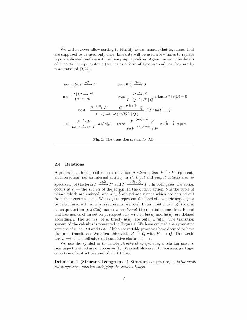
The Asynchronous Local π-calculus (ALπ) [12] is built from the operators ofinaction, input prefix, output, parallel composition, restriction, and replication:

P := 0 | a(b).P | a〈b〉 | P1 | P2 | νa P | !a(b).P .

with the syntactic constraint that in processes a(b).P and !a(b).P names b maynot occur free in P in input position.

When the tilde is empty, the surrounding brackets () and 〈〉 will be omitted.

0 is the inactive process. An input-prefixed process a(b).P , where b has pairwisedistinct components, waits for a tuple of names c to be sent along a and thenbehaves like P{c/b}, where {c/b} is the simultaneous substitution of names b with

names c. An output particle a〈b〉 emits names b at a. Parallel composition isto run two processes in parallel. The restriction νa P makes name a local, orprivate, to P . A replication !P stands for a countable infinite number of copiesof P in parallel. We assign parallel composition the lowest precedence amongthe operators.

2.2 Terminologies and notations

We write a(b). b(c).Q as an abbreviation for νb (ab | b(c).Q), and similarly for

a(b). !b(c).Q. The prefix ‘a(b)’ is called a bound output. In prefixes a(b) and a〈b〉,we call a the subject and b the object. We use α to range over prefixes. Weoften abbreviate α. 0 as α, and νa νb P as (νa, b) P . An input prefix a(b).P

and a restriction νb P are binders for names b and b, respectively, and give risein the expected way to the definition of free names (fn), bound names (bn) andnames (n) of a term or a prefix, and alpha conversion. We identify processes oractions that only differ on the choice of the bound names. The symbol = will

mean “syntactic identity modulo alpha conversion”. Sometimes, we usedef= as

abbreviation mechanism, to assign a name to an expression to which we wantto refer later. In a statement, a name declared fresh is supposed to be differentfrom any other name appearing in the objects of the statement, like processes or

substitutions. Substitutions are of the form {b/c}, and are finite assignments ofnames to names. A context is a process expression with a hole [·] in it. We useC to range over contexts; then C[P ] is the process obtained from C by filling itshole with P .

2.3 Sorting

Following Milner [13], we only admit well-sorted agents, that is agents obeyinga predefined sorting discipline in their manipulation of names. The sortingprevents arity mismatching in communications, like in a〈b, c〉 | a(x).Q. A sortingis an assignment of sorts to names, which specifies the arity of each name and,recursively, of the names carried by that name. We do not present the formalsystem of sorting because it is not essential in the exposition of the topics in thepresent paper.

4

We will however allow sorting to identify linear names, that is, names thatare supposed to be used only once. Linearity will be used a few times to replaceinput-replicated prefixes with ordinary input prefixes. Again, we omit the detailsof linearity in type systems (sorting is a form of type system), as they are bynow standard [9, 24].

inp: a(b).Pa(b)−−−→ P out: a〈b〉 a〈b〉−−−→ 0

rep:P | !P µ−→ P ′

!Pµ−→ P ′

par:P

µ−→ P ′

P | Q µ−→ P ′ | Qif bn(µ) ∩ fn(Q) = ∅

com:P

a(c)−−−→ P ′ Q(ν d) a〈b〉−−−−−−→ Q′

P | Q τ−→ νd (P ′{b/c} | Q′)if d ∩ fn(P ) = ∅

res:P

µ−→ P ′

νa Pµ−→ νa P ′

a 6∈ n(µ) open:P

(ν d) a〈b〉−−−−−−→ P ′

νc P(ν c,d) a〈b〉−−−−−−−→ P ′

c ∈ b− d, a 6= c.

Fig. 1. The transition system for ALπ

2.4 Relations

A process has three possible forms of action. A silent action Pτ−→ P ′ represents

an interaction, i.e. an internal activity in P . Input and output actions are, re-

spectively, of the form Pa(d)−−−→ P ′ and P

(ν d) a〈b〉−−−−−−→ P ′ . In both cases, the actionoccurs at a — the subject of the action. In the output action, b is the tuple ofnames which are emitted, and d ⊆ b are private names which are carried outfrom their current scope. We use µ to represent the label of a generic action (not

to be confused with α, which represents prefixes). In an input action a(d) and in

an output action (ν d) a〈b〉, names d are bound, the remaining ones free. Boundand free names of an action µ, respectively written bn(µ) and fn(µ), are definedaccordingly. The names of µ, briefly n(µ), are bn(µ) ∪ fn(µ). The transitionsystem of the calculus is presented in Figure 1. We have omitted the symmetricversions of rules par and com. Alpha convertible processes have deemed to havethe same transitions. We often abbreviate P

τ−→ Q with P −→ Q. The ‘weak’arrow =⇒ is the reflexive and transitive closure of −→.

We use the symbol ≡ to denote structural congruence, a relation used torearrange the structure of processes [13]. We shall also use it to represent garbage-collection of restrictions and of inert terms.

Definition 1 (Structural congruence). Structural congruence, ≡, is the small-est congruence relation satisfying the axioms below:

5

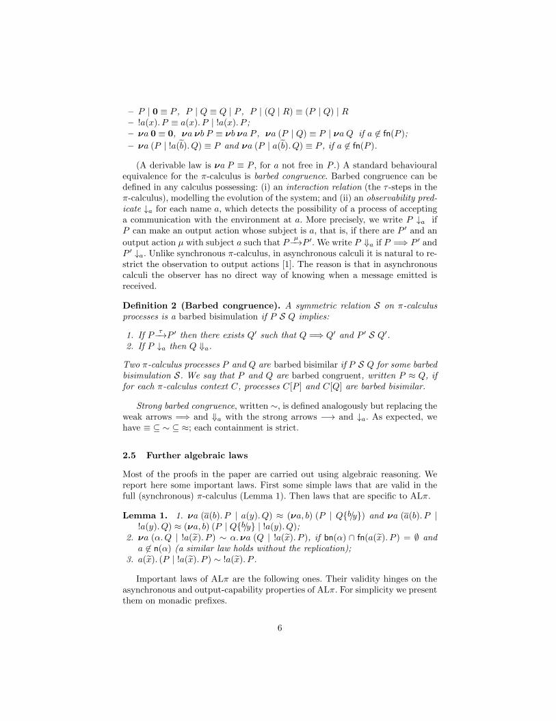
– P | 0 ≡ P , P | Q ≡ Q | P , P | (Q | R) ≡ (P | Q) | R– !a(x).P ≡ a(x).P | !a(x).P ;– νa 0 ≡ 0, νa νb P ≡ νb νa P , νa (P | Q) ≡ P | νa Q if a 6∈ fn(P );

– νa (P | !a(b).Q) ≡ P and νa (P | a(b).Q) ≡ P , if a 6∈ fn(P ).

(A derivable law is νa P ≡ P , for a not free in P .) A standard behaviouralequivalence for the π-calculus is barbed congruence. Barbed congruence can bedefined in any calculus possessing: (i) an interaction relation (the τ -steps in theπ-calculus), modelling the evolution of the system; and (ii) an observability pred-icate ↓a for each name a, which detects the possibility of a process of acceptinga communication with the environment at a. More precisely, we write P ↓a ifP can make an output action whose subject is a, that is, if there are P ′ and an

output action µ with subject a such that Pµ−→P ′. We write P ⇓a if P =⇒ P ′ and

P ′ ↓a. Unlike synchronous π-calculus, in asynchronous calculi it is natural to re-strict the observation to output actions [1]. The reason is that in asynchronouscalculi the observer has no direct way of knowing when a message emitted isreceived.

Definition 2 (Barbed congruence). A symmetric relation S on π-calculusprocesses is a barbed bisimulation if P S Q implies:

1. If Pτ−→P ′ then there exists Q′ such that Q =⇒ Q′ and P ′ S Q′.

2. If P ↓a then Q ⇓a.

Two π-calculus processes P and Q are barbed bisimilar if P S Q for some barbedbisimulation S. We say that P and Q are barbed congruent, written P ≈ Q, iffor each π-calculus context C, processes C[P ] and C[Q] are barbed bisimilar.

Strong barbed congruence, written ∼, is defined analogously but replacing theweak arrows =⇒ and ⇓a with the strong arrows −→ and ↓a. As expected, wehave ≡ ⊆ ∼ ⊆ ≈; each containment is strict.

2.5 Further algebraic laws

Most of the proofs in the paper are carried out using algebraic reasoning. Wereport here some important laws. First some simple laws that are valid in thefull (synchronous) π-calculus (Lemma 1). Then laws that are specific to ALπ.

Lemma 1. 1. νa (a(b).P | a(y).Q) ≈ (νa, b) (P | Q{b/y}) and νa (a(b).P |!a(y).Q) ≈ (νa, b) (P | Q{b/y} | !a(y).Q);

2. νa (α.Q | !a(x).P ) ∼ α.νa (Q | !a(x).P ), if bn(α) ∩ fn(a(x).P ) = ∅ anda 6∈ n(α) (a similar law holds without the replication);

3. a(x). (P | !a(x).P ) ∼ !a(x).P .

Important laws of ALπ are the following ones. Their validity hinges on theasynchronous and output-capability properties of ALπ. For simplicity we presentthem on monadic prefixes.

6

Lemma 2. We have ab ≈ νc (ac | !c(x). bx). Moreover, if b is linear, then thereplication can be removed thus: ab ≈ νc (ac | c(x). bx).

Next, we report some distributivity laws for private replications, i.e., forsystems of the form

νy (P | !y(q).Q)

in which y may occur free in P and Q only in output position. One should thinkof Q as a private resource of P , for P is the only process who can access Q;indeed P can activate as many copies of Q as needed. One such law has alreadybeen given as Lemma 1(2). (The laws can be generalised to the full π-calculus,but need stronger assumptions.)

Lemma 3. Suppose a occurs free in P,R,Q only in output position. Then:

1. νa (P | R | !a(b).Q) ∼ νa (P | !a(b).Q) | νa (R | !a(b).Q);

2. νa ((!P ) | !a(b).Q) ∼ !νa (P | !a(b).Q);

3. νa (α.P | !a(b).Q) ∼ α.νa (P | !a(b).Q), if bn(α) ∩ fn(a(b).Q) = ∅ anda 6∈ n(α);

4. νa ((νc P ) | !a(b).Q) ∼ νc νa (P | !a(b).Q) if c 6∈ fn(a(b).Q).

ALπ has also sharper properties concerning labelled characterisation of bisim-ilarity and associated congruence properties [12, 3].

3 The λ-calculus

We use M,N to range over the set Λ of λ-terms, and x, y, z to range overvariables. The set Λ of λ-terms is given by the grammar:

M ::= x | λx.M | MN

A redex is a term of the form (λx.M)N , and then its contractum is M{N/x}. Incall-by-name evaluation [19], the redex is always at the extreme left of a term.We omit the standard evaluation rules.

Call-by-need [28, 2] optimises call-by-name as follows, so to guarantee that inthe contractum M{N/x} the evaluation of N is not performed more than once.Roughly, N is placed in an environment, and the evaluation continues on M .When x is needed (i.e., x reaches the leftmost position), then N is evaluated and,if a value (i.e., an abstraction) is obtained, say V , then V replaces x (value V canreplace all occurrences of x or, more commonly, only the leftmost occurrence,and then other occurrences of x when they reach the outermost position). Call-by-need is best presented in a graph; or in a system with a let construct torepresent sharing. We refer to Ariola et al. [2] for details, as they are not essentialfor understanding the remainder of the paper; see also the references in Section 5.

We sometimes omit λ in nested abstractions, thus for example, λx1x2.Mstands for λx1.λx2.M . We assume the standard concepts of free and bound

7

variables and substitutions, and identify α-convertible terms. Thus, throughoutthe paper ‘=’ is syntactic equality modulo α-conversion.

Following the call-by-value terminology, the set of abstractions and variablesare the values. (Indeed, call-by-need may also be thought of as a modified formof call-by-value, in which the evaluation of the argument of a function λx.M ismade only when x is used for the first time, rather than before performing thereduction.)

4 The encoding and its properties

4.1 Background material

Figure 2 presents the call-by-name and call-by-need encodings [16, 24]. The call-by-name one is a variant of the original encoding by Milner [14], with the ad-vantage that it can be written in ALπ and can be easily modified to followcall-by-need.

We explain the encodings. The important part is the treatment of application.Both in call-by-name and in call-by-need, a function located at q (its ‘location’)is a process that signals to be a function on q, and then receives a pointer x tothe argument N together with the location p for the next interaction. Now theevaluation of M continues. The difference between call-by-name and call-by-needarises when the argument N is needed. This is signaled by an output at x thatalso provides the location for the evaluation of a copy of N . In call-by-name,every output at x triggers the evaluation of a new copy of N . In call-by-need, incontrast, the evaluation is made only the first time. Precisely, in call-by-need Nis evaluated at the first request and, when it becomes a value, a pointer to thisvalue is returned (instantiating w, in the table). This pointer is returned to theprocess that requested N . When further requests for N are made, the pointeris returned immediately. Thus, for instance, in the call-by-name encoding of(λ.xx)(II) term II is evaluated twice, whereas in the call-by-need encodingonly once. In all encodings, the location names (in the table, the names rangedover by p, q, r) are linear.

Correcteness of call-by-name has been studied in depth. In particular, ithas been shown that β-reduction is validated by the encoding, that the encod-ing gives rise to a term model for the λ-calculus, and that the equivalence onλ-terms induced by the encoding corresponds to the best tree-structures of theλ-calculus — which are also at the heart of its denotational semantics — namelyBohm Trees and Levy-Longo Trees [14, 23] Correctness of the call-by-need encod-ing has been studied only by Brock and Ostheimer [5], and only for operationalcorrespondence with respect to Ariola et al.’s system [2]. (The encoding in Fig-ure 2 is actually a minor improvement over that in [5] — avoiding one reductionstep during a β-reducition — and maintains the results of operational correspon-dence in [5] recalled below.) Following Ariola et al.’s system [2] we write M ⇓if the call-by-need computation of M terminates, and M ⇑ it the computationdoes not terminate.

8

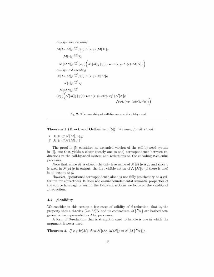
call-by-name encoding

M[[λx.M ]]pdef= p(v). !v(x, q).M[[M ]]q

M[[x]]pdef= xp

M[[MN ]]pdef= (νq )

(M[[M ]]q | q(v).νx v〈x, p〉. !x(r).M[[N ]]r

)call-by-need encoding

N [[λx.M ]]pdef= p(v). !v(x, q).N [[M ]]q

N [[x]]pdef= xp

N [[MN ]]pdef=

(νq )

(N [[M ]]q | q(v).νx v〈x, p〉.x(r).νq′ (N [[N ]]q′ |

q′(w). (rw | !x(r′). r′w))

)

Fig. 2. The encoding of call-by-name and call-by-need

Theorem 1 (Brock and Ostheimer, [5]). We have, for M closed:

1. M ⇓ iff N [[M ]]p ⇓p;2. M ⇑ iff N [[M ]]p ⇑.

The proof in [5] considers an extended version of the call-by-need systemin [2], one that yields a closer (nearly one-to-one) correspondence between re-ductions in the call-by-need system and reductions on the encoding π-calculusprocesses.

Note that, since M is closed, the only free name of N [[M ]]p is p; and since pis used in N [[M ]]p in output, the first visible action of N [[M ]]p (if there is one)is an output at p.

However, operational correspondence alone is not fully satisfactory as a cri-terium for correctness. It does not ensure foundamental semantic properties ofthe source language terms. In the following sections we focus on the validity ofβ-reduction.

4.2 β-validity

We consider in this section a few cases of validity of β-reduction; that is, theproperty that a β-redex (λx.M)N and its contractum M{N/x} are barbed con-gruent when represented as ALπ processes.

A form of β-reduction that is straightforward to handle is one in which theargument is never used.

Theorem 2. If x 6∈ fv(M) then N [[(λx.M)N ]]p ≈ N [[M{N/x}]]p.

9

A more interesting form deals with β-reduction between closed values.

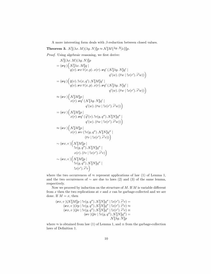
Theorem 3. N [[(λx.M)(λy.N)]]p ≈ N [[M{λy.N/x}]]p.

Proof. Using algebraic reasoning, we first derive:

N [[(λx.M)(λy.N)]]p

= (νq )(N [[λx.M ]]q |q(v).νx v〈x, p〉.x(r).νq′ (N [[λy.N ]]q′ |

q′(w). (rw | !x(r′). r′w)))

= (νq )(q(v). !v(x, q′).N [[M ]]q′ |q(v).νx v〈x, p〉.x(r).νq′ (N [[λy.N ]]q′ |

q′(w). (rw | !x(r′). r′w)))

≈ (νx )(N [[M ]]p |x(r).νq′ (N [[λy.N ]]q′ |

q′(w). (rw | !x(r′). r′w)))

= (νx )(N [[M ]]p |x(r).νq′ ( q′(v). !v(y, q′′).N [[N ]]q′′ |

q′(w). (rw | !x(r′). r′w)))

≈ (νx )(N [[M ]]p |x(r).νv ( !v(y, q′′).N [[N ]]q′′ |

(rv | !x(r′). r′v)))

∼ (νx, v )(N [[M ]]p |!v(y, q′′).N [[N ]]q′′ |x(r). (rv | !x(r′). r′v)

)∼ (νx, v )

(N [[M ]]p |!v(y, q′′).N [[N ]]q′′ |!x(r′). r′v

)where the two occurrences of ≈ represent applications of law (1) of Lemma 1,and the two occurrences of ∼ are due to laws (2) and (3) of the same lemma,respectively.

Now we proceed by induction on the structure of M . If M is variable differentfrom x then the two replications at v and x can be garbage-collected and we aredone. If M = x, then

(νx, v )(N [[M ]]p | !v(y, q′′).N [[N ]]q′′ | !x(r′). r′v) =(νx, v )(xp | !v(y, q′′).N [[N ]]q′′ | !x(r′). r′v) ≈(νx, v )(pv | !v(y, q′′).N [[N ]]q′′ | !x(r′). r′v) ≡

(νv )(pv | !v(y, q′′).N [[N ]]q′′) =N [[λy.N ]]p

where ≈ is obtained from law (1) of Lemma 1, and ≡ from the garbage-collectionlaws of Definition 1.

10

When M is an abstraction or an application, we proceed by induction andexploit the distributivity properties of private replications in Lemma 3

Finally we consider the case when the argument of the function is divergent —a form of β-reduction that is not valid in call-by-value.

Theorem 4. Suppose (λx.M)N is closed. If N ⇑ then we have N [[(λx.M)N ]]p ≈N [[M{N/x}]]p.

Proof. Using Theorem 1 we have N [[N ]]q ⇑, for any q, hence N [[N ]]q ≈ 0. As aconsequence, using algebraic reasoning similar to that in the proof of Theorem 3,we obtain

N [[(λx.M)N ]]p ≈ νx (N [[M ]]p | x(r). 0)

Now, since x occurs in N [[M ]]p only in output subject position, each output atx, say xr, can be removed, or replaced by N [[N ]]r (because in the relation ≈with 0), up-to ≈. This yields N [[M{N/x}]]p.

4.3 Failure of general β-validity

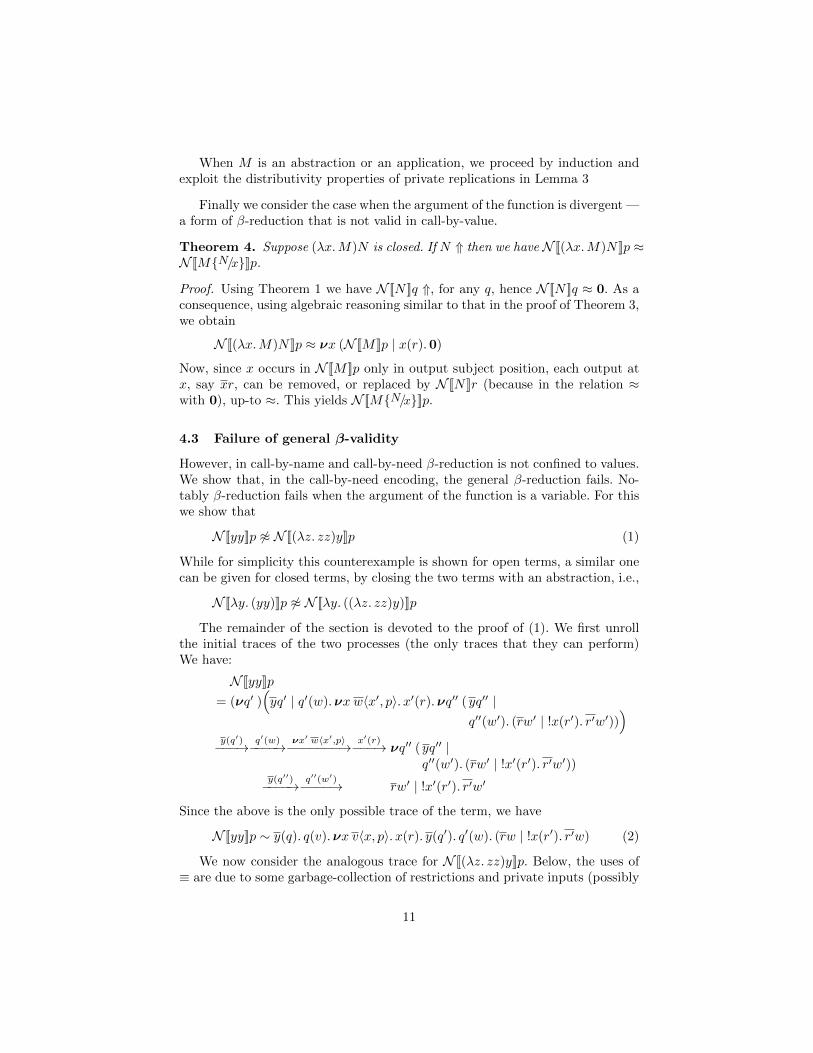
However, in call-by-name and call-by-need β-reduction is not confined to values.We show that, in the call-by-need encoding, the general β-reduction fails. No-tably β-reduction fails when the argument of the function is a variable. For thiswe show that

N [[yy]]p 6≈ N [[(λz. zz)y]]p (1)

While for simplicity this counterexample is shown for open terms, a similar onecan be given for closed terms, by closing the two terms with an abstraction, i.e.,

N [[λy. (yy)]]p 6≈ N [[λy. ((λz. zz)y)]]p

The remainder of the section is devoted to the proof of (1). We first unrollthe initial traces of the two processes (the only traces that they can perform)We have:

N [[yy]]p

= (νq′ )(yq′ | q′(w).νx w〈x′, p〉.x′(r).νq′′ (yq′′ |

q′′(w′). (rw′ | !x(r′). r′w′)))

y(q′)−−−→ q′(w)−−−−→ νx′ w〈x′,p〉−−−−−−−→ x′(r)−−−→ νq′′ (yq′′ |q′′(w′). (rw′ | !x′(r′). r′w′))

y(q′′)−−−−→ q′′(w′)−−−−→ rw′ | !x′(r′). r′w′

Since the above is the only possible trace of the term, we have

N [[yy]]p ∼ y(q). q(v).νx v〈x, p〉.x(r). y(q′). q′(w). (rw | !x(r′). r′w) (2)

We now consider the analogous trace for N [[(λz. zz)y]]p. Below, the uses of≡ are due to some garbage-collection of restrictions and private inputs (possibly

11

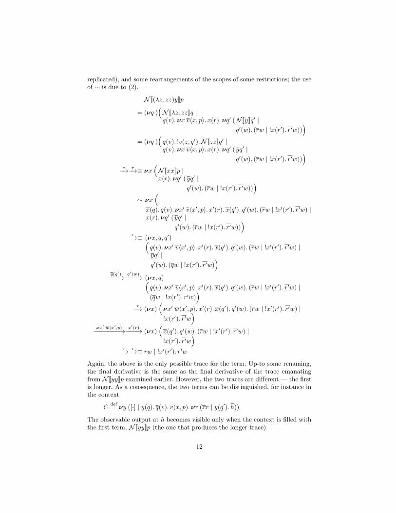
replicated), and some rearrangements of the scopes of some restrictions; the useof ∼ is due to (2).

N [[(λz. zz)y]]p

= (νq )(N [[λz. zz]]q |q(v).νx v〈x, p〉.x(r).νq′ (N [[y]]q′ |

q′(w). (rw | !x(r′). r′w)))

= (νq )(q(v). !v(z, q′).N [[zz]]q′ |q(v).νx v〈x, p〉.x(r).νq′ (yq′ |

q′(w). (rw | !x(r′). r′w)))

τ−→ τ−→≡ νx(N [[xx]]p |x(r).νq′ (yq′ |

q′(w). (rw | !x(r′). r′w)))

∼ νx(

x(q). q(v).νx′ v〈x′, p〉.x′(r).x(q′). q′(w). (rw | !x′(r′). r′w) |x(r).νq′ (yq′ |

q′(w). (rw | !x(r′). r′w)))

τ−→≡ (νx, q, q′)(q(v).νx′ v〈x′, p〉.x′(r).x(q′). q′(w). (rw | !x′(r′). r′w) |yq′ |q′(w). (qw | !x(r′). r′w)

)y(q′)−−−→ q′(w)−−−−→ (νx, q)(

q(v).νx′ v〈x′, p〉.x′(r).x(q′). q′(w). (rw | !x′(r′). r′w) |(qw | !x(r′). r′w)

)τ−→ (νx)

(νx′ w〈x′, p〉.x′(r).x(q′). q′(w). (rw | !x′(r′). r′w) |!x(r′). r′w

)νx′ w〈x′,p〉−−−−−−−→ x′(r)−−−→ (νx)

(x(q′). q′(w). (rw | !x′(r′). r′w) |!x(r′). r′w

)τ−→ τ−→≡ rw | !x′(r′). r′w

Again, the above is the only possible trace for the term. Up-to some renaming,the final derivative is the same as the final derivative of the trace emanatingfrom N [[yy]]p examined earlier. However, the two traces are different — the firstis longer. As a consequence, the two terms can be distinguished, for instance inthe context

Cdef= νy ([·] | y(q). q(v). v(x, p).νr (xr | y(q′).h))

The observable output at h becomes visible only when the context is filled withthe first term, N [[yy]]p (the one that produces the longer trace).

12

In contrast, in the call-by-name encoding the validity of the full β-reductionholds [23]. Therefore the above counterexample not only shows that the call-by-need encoding is observably different from the call-by-name one; it also tells usthat the properties that the two encoding satisfy are quite different.

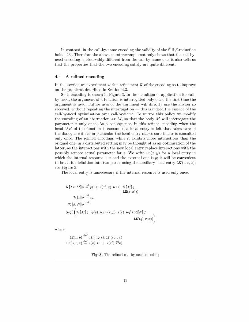
4.4 A refined encoding

In this section we experiment with a refinement R of the encoding so to improveon the problems described in Section 4.3.

Such encoding is shown in Figure 3. In the definition of application for call-by-need, the argument of a function is interrogated only once, the first time theargument is used. Future uses of the argument will directly use the answer soreceived, without repeating the interrogation — this is indeed the essence of thecall-by-need optimisation over call-by-name. To mirror this policy we modifythe encoding of an abstraction λx.M , so that the body M will interrogate theparameter x only once. As a consequence, in this refined encoding when thehead ‘λx’ of the function is consumed a local entry is left that takes care ofthe dialogue with x; in particular the local entry makes sure that x is consultedonly once. The refined encoding, while it exhibits more interactions than theoriginal one, in a distributed setting may be thought of as an optimisation of thelatter, as the interactions with the new local entry replace interactions with thepossibly remote actual parameter for x. We write LE(x, y) for a local entry inwhich the internal resource is x and the external one is y; it will be convenientto break its definition into two parts, using the auxiliary local entry LE′(s, r, x);see Figure 3.

The local entry is unnecessary if the internal resource is used only once.

R[[λx.M ]]pdef= p(v). !v(x′, q).νx ( R[[M ]]q

| LE(x, x′))

R[[x]]pdef= xp

R[[MN ]]pdef=

(νq )

(R[[M ]]q | q(v).νx v〈x, p〉.x(r).νq′ (R[[N ]]q′ |

LE′(q′, r, x))

)where

LE(x, y)def= x(r). y(s). LE′(s, r, x)

LE′(s, r, x)def= s(v). (rv | !x(r′). r′v)

Fig. 3. The refined call-by-need encoding

13

Lemma 4. Suppose z′ appears only once in M . Then

νz′ (R[[M ]]p | LE(z′, z)) ≈ R[[M{z/z′}]]p

Proof. By induction on the structure of M . The most interesting case is whenM = z′, in which case we exploit the (linear) law of ALπ in Lemma 2. When Mis an application we exploit the hypothesis (z′ occurring only once), and simplealgebraic manipulation, so to be able to carry out the induction.

The next lemma shows that local entries compose.

Lemma 5. νx (LE(z, x) | LE(x, y)) ≈ LE(z, y).

Proof. We use laws (2) and (1) of Lemma 1, and the garbage-collection laws ofstructural congruence.

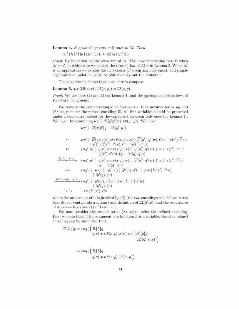
We revisite the counterexample of Section 4.3, that involves terms yy and(λz. zz)y, under the refined encoding R. All free variables should be protectedunder a local entry, except for the variables that occur only once (by Lemma 4).We begin by examining νy′ ( R[[y′y′]]q | LE(y′, y)). We have:

νy′ ( R[[y′y′]]q | LE(y′, y))

∼ νy′ ( y′(q). q(v).νx v〈x, p〉.x(r). y′(q′). q′(w). (rw | !x(r′). r′w)| y′(r). y(r′). r′(v). (rv | !y′(r). rv))

≈ (νy′, q) ( q(v).νx v〈x, p〉.x(r). y′(q′). q′(w). (rw | !x(r′). r′w)| y(r′). r′(v). (qv | !y′(q). qv))

y(r′)−−−→ r′(v)−−−→ (νy′, q) ( q(v).νx v〈x, p〉.x(r). y′(q′). q′(w). (rw | !x(r′). r′w)| qv | !y′(q). qv)

τ−→ (νy′) ( νx v〈x, p〉.x(r). y′(q′). q′(w). (rw | !x(r′). r′w)| !y′(q). qv)

νx v〈x,p〉−−−−−−→ x(r)−−−→ (νy′) ( y′(q′). q′(w). (rw | !x(r′). r′w)| !y′(q). qv)

τ−→ τ−→ rv | !x(r′). r′v

where the occurrence of ∼ is justified by (2) (the two encodings coincide on termsthat do not contain abstractions) and definition of LE(y′, y), and the occurrenceof ≈ comes from law (1) of Lemma 1.

We now consider the second term, (λz. zz)y, under the refined encoding.First we note that, if the argument of a function L is a variable, then the refinedencoding can be simplified thus:

R[[Ly]]p = (νq )(R[[L]]q |q(v).νx v〈x, p〉.x(r).νq′ (N [[y]]q′ |

LE′(q′, r, x)))

= (νq )(R[[L]]q |q(v).νx v〈x, p〉. LE(x, y)

)14

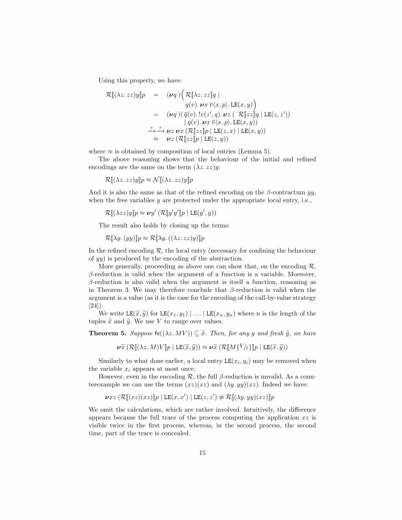
Using this property, we have:

R[[(λz. zz)y]]p = (νq )(R[[λz. zz]]q |q(v).νx v〈x, p〉. LE(x, y)

)= (νq )( q(v). !v(z′, q).νz ( R[[zz]]q | LE(z, z′))

| q(v).νx v〈x, p〉. LE(x, y))τ−→ τ−→ νz νx (R[[zz]]p | LE(z, x) | LE(x, y))≈ νz (R[[zz]]p | LE(z, y))

where ≈ is obtained by composition of local entries (Lemma 5).The above reasoning shows that the behaviour of the initial and refined

encodings are the same on the term (λz. zz)y:

R[[(λz. zz)y]]p ≈ N [[(λz. zz)y]]p

And it is also the same as that of the refined encoding on the β-contractum yy,when the free variables y are protected under the appropriate local entry, i.e.,

R[[(λzz)y]]p ≈ νy′ (R[[y′y′]]p | LE(y′, y))

The result also holds by closing up the terms:

R[[λy. (yy)]]p ≈ R[[λy. ((λz. zz)y)]]p

In the refined encoding R, the local entry (necessary for confining the behaviourof yy) is produced by the encoding of the abstraction.

More generally, proceeding as above one can show that, on the encoding R,β-reduction is valid when the argument of a function is a variable. Moreover,β-reduction is also valid when the argument is itself a function, reasoning asin Theorem 3. We may therefore conclude that β-reduction is valid when theargument is a value (as it is the case for the encoding of the call-by-value strategy[24]).

We write LE(x, y) for LE(x1, y1) | . . . | LE(xn, yn) where n is the length of thetuples x and y. We use V to range over values.

Theorem 5. Suppose fv((λz.MV )) ⊆ x. Then, for any y and fresh y, we have

νx (R[[(λz.M)V ]]p | LE(x, y)) ≈ νx (R[[M{V/z}]]p | LE(x, y))

Similarly to what done earlier, a local entry LE(xi, yi) may be removed whenthe variable xi appears at most once.

However, even in the encoding R, the full β-reduction is unvalid. As a coun-terexample we can use the terms (xz)(xz) and (λy. yy)(xz). Indeed we have:

νxz (R[[(xz)(xz)]]p | LE(x, x′) | LE(z, z′) 6≈ R[[(λy. yy)(xz)]]p

We omit the calculations, which are rather involved. Intuitively, the differenceappears because the full trace of the process computing the application xz isvisible twice in the first process, whereas, in the second process, the secondtime, part of the trace is concealed.

15

5 Conclusions

Call-by-need was proposed by Wadsworth [28] as an implementation technique.Formalizations of call-by-need on a λ-calculus with a let construct or withenvironments include Ariola et al. [2], Launchbury [11], Purushothaman andSeaman [20], and Yoshida [29]. The uniform encoding in Section 4 is from [16].A study of the correctness of the call-by-need encoding in Figure 2 is in [5].Encodings of graph reductions, related to call-by-need, into π-calculus were givenin [4, 8] but their correctness was not studied. Niehren [15] used encodings of call-by-name, call-by-value and call-by-need λ-calculi into π-calculus to compare thetime complexity of the strategies.

In the paper we have used the theory of the Asynchronous Local π-calculus(ALπ) [12] to reason about the encoding of the call-by-need λ-calculus strategyas processes. We have mainly focused on the validity of β-reduction. We haveshowed that various instances of the property on closed terms hold, though thegeneral property fails. We have also considered a refined encoding in which β-reduction on arbitrary values (though not on arbitrary terms) holds. All thisleaves us with some challenging questions, that we leave for future work:

1. In the refined encoding, we use special processes called local entries to protectthe formal parameter of the function, thus improving the results about β-validity. Is it possible to further protect variables (or terms) so to recoverthe full β-validity?

2. Is there a different form of behavioural equivalence under which the fullβ-validity holds, in the initial or in the refined encoding?

3. What is an appropriate process preorder under which call-by-need can indeedbe proved to be an optimisation of call-by-name?

4. What is the equivalence on λ-terms induced by the call-by-need encoding?Following the results for call-by-name and call-by-value, one expects to re-cover some kind of tree structure (Bohm Trees and Levy-Longo Tree forcall-by-name, Lassen’s trees [10] for call-by-value). We are not aware of sim-ilar tree structures for call-by-need. Hence investigating this question mayalso shed light on what should the appropriate forms of trees for call-by-needbe.

In questions (2) and (3), ‘easy’ answers may be obtained by confining thetesting contexts to be encodings of λ-calculus contexts. The challenge is to findmore general and useful answers, with applications outside the realm of pureλ-calculi. One may consider forms of behavioural types.

In questions (1) and (2), perhaps requiring the validity of the full β-reduction,in the same way as for call-by-name, is too demanding. Indeed in this wayprobably the tree structure referred to in question (4) is likely to be the same asthat for call-by-name. One may find it acceptable to limit β-validity to reductionsbetween closed terms.

16

Acknowledgments Thanks to the reviewers for their careful reading of the pa-per and their suggestions. Research partly supported by the H2020-MSCA-RISEproject ID 778233 “Behavioural Application Program Interfaces (BEHAPI)”.

References

1. Amadio, R., Castellani, I., Sangiorgi, D.: On bisimulations for the asynchronousπ-calculus. Theoretical Computer Science 195, 291–324 (1998)

2. Ariola, Z., Felleisen, M., Maraist, J., Odersky, M., Wadler, P.: A call-by-need λ-calculus. In: Proc. 22th POPL. ACM Press (1995)

3. Boreale, M., Sangiorgi, D.: Some congruence properties for π-calculus bisimilarities.Theoretical Computer Science 198, 159–176 (1998)

4. Boudol, G.: Some chemical abstract machines. In: Proc. REX SummerSchool/Symposium 1993. Lecture Notes in Computer Science, vol. 803. SpringerVerlag (1994)

5. Brock, S., Ostheimer, G.: Process semantics of graph reduction. In: Lee, I., Smolka,S. (eds.) Proc. CONCUR ’95. Lecture Notes in Computer Science, vol. 962, pp.471–485. Springer Verlag, Philadelphia, Pennsylvania (1995)

6. Durier, A., Hirschkoff, D., Sangiorgi, D.: Eager functions as processes. In: 33ndAnnual ACM/IEEE Symposium on Logic in Computer Science, LICS 2018. IEEEComputer Society (2018)

7. Fournet, C., Gonthier, G.: The join calculus: A language for distributed mobileprogramming. In: Barthe, G., Dybjer, P., Pinto, L., Saraiva, J. (eds.) Applied Se-mantics, International Summer School, APPSEM 2000. Lecture Notes in ComputerScience, vol. 2395, pp. 268–332. Springer (2002)

8. Jeffrey, A.: A chemical abstract machine for graph reduction. In: Proc. Ninth Inter-national Conference on the Mathematical Foundations of Programming Semantics(MFPS’93). Lecture Notes in Computer Science, vol. 802. Springer Verlag (1993)

9. Kobayashi, N., Pierce, B., Turner, D.: Linearity and the pi-calculus. TOPLAS21(5), 914–947 (1999), preliminary summary appeared in Proceedings of POPL’96

10. Lassen, S.B.: Eager normal form bisimulation. In: 20th IEEE Symposium on Logicin Computer Science (LICS 2005), 26-29 June 2005, Chicago, IL, USA, Proceedings.pp. 345–354 (2005)

11. Launchbury, J.: A natural semantics for lazy evaluation. In: Proc. 20th POPL.ACM Press (1993)

12. Merro, M., Sangiorgi, D.: On asynchrony in name-passing calculi. Journal of Math-ematical Structures in Computer Science 14(5), 715–767 (2004)

13. Milner, R.: The polyadic π-calculus: a tutorial. Tech. Rep. ECS–LFCS–91–180,LFCS, Dept. of Comp. Sci., Edinburgh Univ. (Oct 1991), Also in Logic and Algebraof Specification, ed. F.L. Bauer, W. Brauer and H. Schwichtenberg, Springer Verlag,1993.

14. Milner, R.: Functions as processes. Journal of Mathematical Structures in Com-puter Science 2(2), 119–141 (1992)

15. Niehren, J.: Functional computation as concurrent computation. In: Proc. 23thPOPL. ACM Press (1996)

16. Ostheimer, G., Davie, A.: π-calculus characterisations of some practical λ-calculusreductions strategies. Tech. Rep. CS/93/14, St. Andrews (1993)

17. Palamidessi, C.: Comparing the expressive power of the synchronous and asyn-chronous pi-calculi. Journal of Mathematical Structures in Computer Science 13(5),685–719 (2003)

17

18. Pierce, B.C., Turner, D.N.: Pict: A programming language based on the pi-calculus.In: Plotkin, G., Stirling, C., Tofte, M. (eds.) Proof, Language and Interaction:Essays in Honour of Robin Milner. MIT Press (2000)

19. Plotkin, G.: Call by name, call by value and the λ-calculus. Theoretical ComputerScience 1, 125–159 (1975)

20. Purushothaman, S., Seaman, J.: An adequate operational semantics for sharing inlazy evaluation. In: Krieg-Bruckner, B. (ed.) ESOP’92. Lecture Notes in ComputerScience, vol. 582, pp. 435–450. Springer Verlag (1992)

21. Sangiorgi, D.: An investigation into functions as processes. In: Proc. Ninth Inter-national Conference on the Mathematical Foundations of Programming Semantics(MFPS’93). Lecture Notes in Computer Science, vol. 802, pp. 143–159. SpringerVerlag (1993)

22. Sangiorgi, D.: From λ to π, or: Rediscovering continuations. Journal of Mathemati-cal Structures in Computer Science 9(4) (1999), special Issue on ”Lambda-Calculusand Logic” in Honour of Roger Hindley

23. Sangiorgi, D.: Lazy functions and mobile processes. In: Plotkin, G., Stirling, C.,Tofte, M. (eds.) Proof, Language and Interaction: Essays in Honour of Robin Mil-ner. MIT Press (2000)

24. Sangiorgi, D., Walker, D.: The π-calculus: a Theory of Mobile Processes. Cam-bridge University Press (2001)

25. Sangiorgi, D.: Typed pi-calculus at work: A correctness proof of Jones’s paralleli-sation transformation on concurrent objects. TAPOS 5(1), 25–33 (1999)

26. Turner, N.: The polymorphic pi-calculus: Theory and Implementation. Ph.D. the-sis, Department of Computer Science, University of Edinburgh (1996)

27. Vasconcelos, V.T.: Lambda and pi calculi, CAM and SECD machines. J. Funct.Program. 15(1), 101–127 (2005)

28. Wadsworth, C.P.: Semantics and pragmatics of the lambda calculus. Ph.D. thesis,University of Oxford (1971)

29. Yoshida, N.: Optimal reduction in weak lambda-calculus with shared environments.In: Proc. of FPCA’93, Functional Programming and Computer Architecture. pp.243–252 (1993)

18