Asynchronous Multi-View SLAM

Anqi Joyce Yang∗1,2, Can Cui∗1,3, Ioan Andrei Bârsan∗1,2, Raquel Urtasun1,2, Shenlong Wang1,2

Abstract— Existing multi-camera SLAM systems assume syn-chronized shutters for all cameras, which is often not thecase in practice. In this work, we propose a generalized multi-camera SLAM formulation which accounts for asynchronoussensor observations. Our framework integrates a continuous-time motion model to relate information across asynchronousmulti-frames during tracking, local mapping, and loop closing.For evaluation, we collected AMV-Bench, a challenging newSLAM dataset covering 482 km of driving recorded using ourasynchronous multi-camera robotic platform. AMV-Bench isover an order of magnitude larger than previous multi-view HDoutdoor SLAM datasets, and covers diverse and challengingmotions and environments. Our experiments emphasize thenecessity of asynchronous sensor modeling, and show that theuse of multiple cameras is critical towards robust and accurateSLAM in challenging outdoor scenes. The supplementary mate-rial is located at: https://www.cs.toronto.edu/~ajyang/amv-slam

I. INTRODUCTION

Simultaneous Localization and Mapping (SLAM) is the

task of localizing an autonomous agent in unseen envi-

ronments by building a map at the same time. SLAM

is a fundamental part of many technologies ranging from

augmented reality to photogrammetry and robotics. Due to

the availability of camera sensors and the rich information

they provide, camera-based SLAM, or visual SLAM, has

been widely studied and applied in robot navigation.

Existing visual SLAM methods [1]–[5] and benchmarks [6]–

[8] mainly focus on either monocular or stereo camera

settings. Although lightweight, such configurations are prone

to tracking failures caused by occlusion, dynamic objects,

lighting changes and textureless scenes, all of which are

common in the real world. Many of these challenges can

be attributed to the narrow field of view typically used

(Fig. 1a). Due to their larger field of view (Fig. 1b), wide-

angle or fisheye lenses [9], [10] or multi-camera rigs [11]–

[16] can significantly increase the robustness of visual SLAM

systems [15].

Nevertheless, using multiple cameras comes with its own

set of challenges. Existing stereo [5] or multi-camera [11]–

[15] SLAM literature assumes synchronized shutters for all

cameras and adopts discrete-time trajectory modeling based

on this assumption. However, in practice different cameras

are not always triggered at the same time, either due to

technical limitations, or by design. For instance, the camera

shutters could be synchronized to another sensor, such as a

∗Denotes equal contribution. Work done during Can’s internship at Uber.1Uber Advanced Technologies Group2University of Toronto,

ajyang, iab, urtasun, slwang@cs.toronto.edu3University of Waterloo, c23cui@uwaterloo.ca

spinning LiDAR (e.g., Fig. 1c), which is a common set-up

in self-driving [17]–[20]. Moreover, failure to account for

the robot motion in between the firing of the cameras could

lead to localization failures. Consider a car driving along a

highway at 30m/s (108km/h). Then in a short 33ms camera

firing interval, the vehicle would travel one meter, which

is significant when centimeter-accurate pose estimation is

required. As a result, a need arises for a generalization of

multi-view visual SLAM to be agnostic to camera timing,

while being scalable and robust to real-world conditions.

In this paper we formalize the asynchronous multi-view

SLAM (AMV-SLAM) problem. Our first contribution is a

general framework for AMV-SLAM, which, to the best of

our knowledge, is the first full asynchronous continuous-time

multi-camera visual SLAM system for large-scale outdoor

environments. Key to this formulation is (1) the concept

of asynchronous multi-frames, which group input images

from multiple asynchronous cameras, and (2) the integration

of a continuous-time motion model, which relates spatio-

temporal information from asynchronous multi-frames for

joint continuous-time trajectory estimation.

Since there is no public asynchronous multi-camera SLAM

dataset, our second contribution is AMV-Bench, a novel large-

scale dataset with high-quality ground-truth. AMV-Bench was

collected during a full year in Pittsburgh, PA, and includes

challenging conditions such as low-light scenes, occlusions,

fast driving (Fig. 1d), and complex maneuvers like three-

point turns and reverse parking. Our experiments show that

multi-camera configurations are critical in overcoming adverse

conditions in large-scale outdoor scenes. In addition, we show

that asynchronous sensor modeling is crucial, as treating the

cameras as synchronous leads to 30% higher failure rate and

4× the local pose errors compared to asynchronous modeling.

II. RELATED WORK

1) Visual SLAM / Visual Odometry: SLAM has been

a core area of research in robotics since 1980s [21]–[25].

The comprehensive survey by Cadena et al. [26] provides

a detailed overview of SLAM. Modern visual SLAM ap-

proaches can be divided into direct and indirect methods.

Direct methods like DTAM [27], LSD-SLAM [1], and

DSO [3] estimate motion and map parameters by directly

optimizing over pixel intensities (photometric error) [28],

[29]. Alternatively, indirect methods, which are the focus

of this work, minimize the re-projection energy (geometric

error) [30] over an intermediate representation obtained from

raw images. A common subset of these are feature-based

methods like PTAM [31] and ORB-SLAM [4] which represent

raw observations as sets of keypoints.

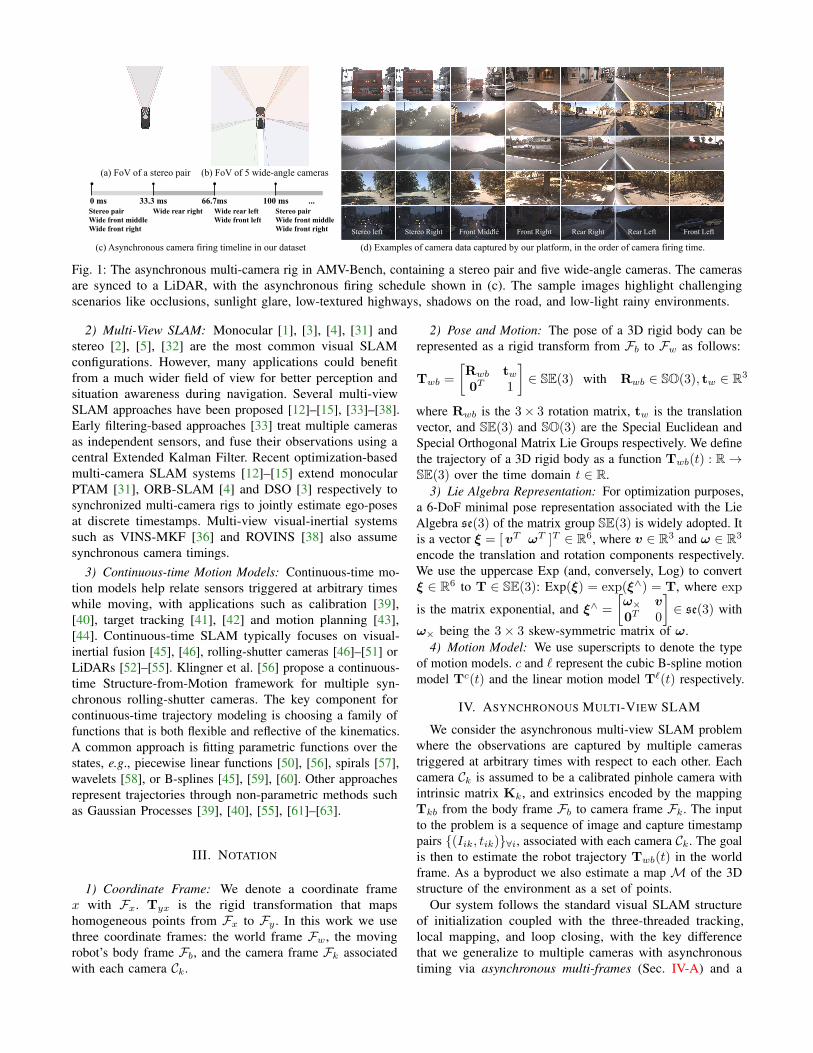
66.7ms 100 ms0 ms 33.3 msWide rear rightStereo pair

Wide front middleWide front right

Wide rear leftWide front left

Stereo pairWide front middleWide front right

...

(a) FoV of a stereo pair (b) FoV of 5 wide-angle cameras

(c) Asynchronous camera firing timeline in our dataset (d) Examples of camera data captured by our platform, in the order of camera firing time.

Stereo left Stereo Right Front Middle Front Right Rear Right Rear Left Front Left

Fig. 1: The asynchronous multi-camera rig in AMV-Bench, containing a stereo pair and five wide-angle cameras. The cameras

are synced to a LiDAR, with the asynchronous firing schedule shown in (c). The sample images highlight challenging

scenarios like occlusions, sunlight glare, low-textured highways, shadows on the road, and low-light rainy environments.

2) Multi-View SLAM: Monocular [1], [3], [4], [31] and

stereo [2], [5], [32] are the most common visual SLAM

configurations. However, many applications could benefit

from a much wider field of view for better perception and

situation awareness during navigation. Several multi-view

SLAM approaches have been proposed [12]–[15], [33]–[38].

Early filtering-based approaches [33] treat multiple cameras

as independent sensors, and fuse their observations using a

central Extended Kalman Filter. Recent optimization-based

multi-camera SLAM systems [12]–[15] extend monocular

PTAM [31], ORB-SLAM [4] and DSO [3] respectively to

synchronized multi-camera rigs to jointly estimate ego-poses

at discrete timestamps. Multi-view visual-inertial systems

such as VINS-MKF [36] and ROVINS [38] also assume

synchronous camera timings.

3) Continuous-time Motion Models: Continuous-time mo-

tion models help relate sensors triggered at arbitrary times

while moving, with applications such as calibration [39],

[40], target tracking [41], [42] and motion planning [43],

[44]. Continuous-time SLAM typically focuses on visual-

inertial fusion [45], [46], rolling-shutter cameras [46]–[51] or

LiDARs [52]–[55]. Klingner et al. [56] propose a continuous-

time Structure-from-Motion framework for multiple syn-

chronous rolling-shutter cameras. The key component for

continuous-time trajectory modeling is choosing a family of

functions that is both flexible and reflective of the kinematics.

A common approach is fitting parametric functions over the

states, e.g., piecewise linear functions [50], [56], spirals [57],

wavelets [58], or B-splines [45], [59], [60]. Other approaches

represent trajectories through non-parametric methods such

as Gaussian Processes [39], [40], [55], [61]–[63].

III. NOTATION

1) Coordinate Frame: We denote a coordinate frame

x with Fx. Tyx is the rigid transformation that maps

homogeneous points from Fx to Fy. In this work we use

three coordinate frames: the world frame Fw, the moving

robot’s body frame Fb, and the camera frame Fk associated

with each camera Ck.

2) Pose and Motion: The pose of a 3D rigid body can be

represented as a rigid transform from Fb to Fw as follows:

Twb =

[Rwb tw

0T 1

]∈ SE(3) with Rwb ∈ SO(3), tw ∈ R

3

where Rwb is the 3× 3 rotation matrix, tw is the translation

vector, and SE(3) and SO(3) are the Special Euclidean and

Special Orthogonal Matrix Lie Groups respectively. We define

the trajectory of a 3D rigid body as a function Twb(t) : R →SE(3) over the time domain t ∈ R.

3) Lie Algebra Representation: For optimization purposes,

a 6-DoF minimal pose representation associated with the Lie

Algebra se(3) of the matrix group SE(3) is widely adopted. It

is a vector ξ = [vT ωT ]T ∈ R6, where v ∈ R

3 and ω ∈ R3

encode the translation and rotation components respectively.

We use the uppercase Exp (and, conversely, Log) to convert

ξ ∈ R6 to T ∈ SE(3): Exp(ξ) = exp(ξ∧) = T, where exp

is the matrix exponential, and ξ∧ =

[ω× v

0T 0

]∈ se(3) with

ω× being the 3× 3 skew-symmetric matrix of ω.

4) Motion Model: We use superscripts to denote the type

of motion models. c and ℓ represent the cubic B-spline motion

model Tc(t) and the linear motion model Tℓ(t) respectively.

IV. ASYNCHRONOUS MULTI-VIEW SLAM

We consider the asynchronous multi-view SLAM problem

where the observations are captured by multiple cameras

triggered at arbitrary times with respect to each other. Each

camera Ck is assumed to be a calibrated pinhole camera with

intrinsic matrix Kk, and extrinsics encoded by the mapping

Tkb from the body frame Fb to camera frame Fk. The input

to the problem is a sequence of image and capture timestamp

pairs (Iik, tik)∀i, associated with each camera Ck. The goal

is then to estimate the robot trajectory Twb(t) in the world

frame. As a byproduct we also estimate a map M of the 3D

structure of the environment as a set of points.

Our system follows the standard visual SLAM structure

of initialization coupled with the three-threaded tracking,

local mapping, and loop closing, with the key difference

that we generalize to multiple cameras with asynchronous

timing via asynchronous multi-frames (Sec. IV-A) and a

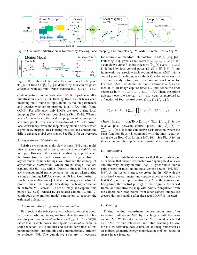
Async MFi

Async MFi Input(Sec IV.A)

time

…

…

𝐼!"

Loop Closing(Sec IV.F)

Local KMFs𝐼!#𝐼!$

𝑡!" 𝑡!# 𝑡!$

Tracking (Sec IV.D)

KMF1

KMF0

KMFref

…

…

Init(Sec IV.C)

KMF?

yes

no

Local Mapping (Sec IV.E)

…

…

BA

Loop?

yes

no

Matched Image

Next MF

Fig. 2: Overview. Initialization is followed by tracking, local mapping and loop closing. MF=Multi-Frame; KMF=Key MF.

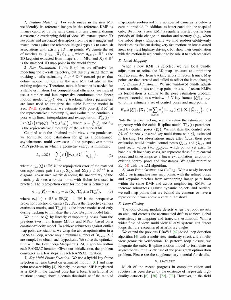
Motion Model

(Sec IV.B)

Control Point

time

spac

e 𝜉!"#

$ 𝜉!

$𝜉!%&

$𝜉!%#

$

𝑡! 𝑡!"#𝒕 𝑡!"$

……

𝑡!%#

SE(3) Spline

Fig. 3: Illustration of the cubic B-spline model. The pose

Tcwb(t) at time t ∈ [ti, ti+1] is defined by four control poses

associated with key multi-frames indexed at i−1, i, i+1, i+2.

continuous-time motion model (Sec. IV-B). In particular, after

initialization (Sec. IV-C), tracking (Sec. IV-D) takes each

incoming multi-frame as input, infers its motion parameters,

and decides whether to promote it as a key multi-frame

(KMF). For efficiency, only KMFs are used during local

mapping (Sec. IV-E) and loop closing (Sec. IV-F). When a

new KMF is selected, the local mapping module refines poses

and map points over a recent window of KMFs to ensure

local consistency, while the loop closing module detects when

a previously-mapped area is being revisited and corrects the

drift to enhance global consistency. See Fig. 2 for an overview.

A. Asynchronous Multi-Frames

Existing synchronous multi-view systems [14] group multi-

view images captured at the same time into a multi-frame

as input. However, this cannot be directly applied when

the firing time of each sensor varies. To generalize to

asynchronous camera timings, we introduce the concept of

asynchronous multi-frame, which groups images that are

captured closely (e.g., within 100ms) in time. In Fig. 1 each

asynchronous multi-frame contains the images taken during

a single spinning LiDAR sweep at 10 Hz. Contrasting to

synchronous multi-frames [14] that store images and a discrete

pose estimated at a single timestamp, each asynchronous

multi-frame MFi stores: (1) a set of image and capture time

pairs (Iik, tik) indexed by associated camera Ck, and (2)

continuous-time motion model parameters to recover the

estimated trajectory.

B. Continuous-Time Trajectory Representation

To associate the robot pose with observations that could

be made at arbitrary times, we formulate the overall robot

trajectory as a continuous-time function Twb(t) : R → SE(3),rather than discrete poses. We exploit a cumulative cubic B-

spline function [45] as the first and second derivatives of this

parameterization are smooth and computationally efficient

to evaluate [59]. The cumulative structure is necessary

for accurate on-manifold interpolation in SE(3) [45], [64].

Following [45], given a knot vector b = [t0, t1, . . . , t7] ∈ R8,

a cumulative cubic B-spline trajectory Tcwb(t) over t ∈ [t3, t4)

is defined by four control poses ξc0 : ξc3 ∈ R

6 [45]. In our

framework, we associate each key multi-frame KMFi with a

control pose. In addition, since the KMFs do not necessarily

distribute evenly in time, we use a non-uniform knot vector.

For each KMFi, we define the representative time ti as the

median of all image capture times tik, and define the knot

vector as bi = [ti−3, ti−2, . . . , ti+4] ∈ R8. Then, the spline

trajectory over the interval t ∈ [ti, ti+1) can be expressed as

a function of four control poses ξci−1, ξci , ξci+1, ξci+2:

Tcwb(t) = Exp

(ξci−1

) 3∏

j=1

Exp(Bj,4(t)ΩΩΩi−1+j

), (1)

where ΩΩΩi−1+j = Log(Exp(ξci−2+j)−1Exp(ξci−1+j)) is the

relative pose between control poses, and Bj,4(t) =∑3l=j Bl,4(t) ∈ R is the cumulative basis function, where the

basis function Bl,4(t) is computed with the knot vector bi

using the de Boor-Cox formula [65], [66]. See Fig. 3 for an

illustration, and the supplementary material for more details.

C. Initialization

The system initialization assumes that there exists a pair

of cameras that share a reasonable overlapping field of view

and fire very closely in time (e.g., a synchronous stereo

pair, present in most autonomous vehicle setups [19], [67],

[68]). At the system startup, we create the first MF with the

associated camera images and capture times, select it as the

first KMF, set the representative time t0 to the camera pair

firing time, the control pose ξc0 to the origin of the world

frame, and initialize the map with points triangulated from

the camera pair. Map points from other camera images are

created during mapping after the second KMF is inserted.

D. Tracking

During tracking, we estimate the continuous pose of an

incoming multi-frame MFi by matching it with the most

recent KMF. We then decide whether MFi should be selected

as a KMF for map refinement and future tracking. Follow-

ing [4], we formulate pose estimation and map refinement as

an indirect geometric energy minimization problem based on

sparse image features.

1) Feature Matching: For each image in the new MF,

we identify its reference images in the reference KMF as

images captured by the same camera or any camera sharing

a reasonable overlapping field of view. We extract sparse 2D

keypoints and associated descriptors from the new images and

match them against the reference image keypoints to establish

associations with existing 3D map points. We denote the set

of matches as (ui,k,j ,Xj)∀(k,j), where ui,k,j ∈ R2 is the

2D keypoint extracted from image Iik in MFi, and Xj ∈ R3

is the matched 3D map point in the world frame.

2) Pose Estimation: Cubic B-splines are effective for

modeling the overall trajectory, but directly using them in

tracking entails estimating four 6-DoF control poses that

define motion not only in the new MF, but also in the

existing trajectory. Therefore, more information is needed for

a stable estimation. For computational efficiency, we instead

use a simpler and less expressive continuous-time linear

motion model Tℓwb(t) during tracking, whose parameters

are later used to initialize the cubic B-spline model in

Sec. IV-E. Specifically, we estimate MFi pose ξℓi ∈ R6 at

the representative timestamp ti, and evaluate the continuous

pose with linear interpolation and extrapolation: Tℓwb(t) =

Exp(ξℓi )(

Exp(ξℓi )−1

Tcwb(tref)

)α

, where α = ti−tti−tref

and tref

is the representative timestamp of the reference KMF.

Coupled with the obtained multi-view correspondences,

we formulate pose estimation for ξℓi as a constrained,

asynchronous, multi-view case of the perspective-n-points

(PnP) problem, in which a geometric energy is minimized:

Egeo(ξℓi ) =

∑

(k,j)

ρ(∥∥ei,k,j(ξℓi )

∥∥2Σ

−1

i,k,j

), (2)

where ei,k,j(ξℓi )∈R

2 is the reprojection error of the matched

correspondence pair (ui,k,j ,Xj), and Σi,k,j ∈ R2×2 is a

diagonal covariance matrix denoting the uncertainty of the

match. ρ denotes a robust norm, with Huber loss used in

practice. The reprojection error for the pair is defined as:

ei,k,j(ξℓi ) = ui,k,j − πk

(Xj ,T

ℓwb(tik)T

−1kb

), (3)

where πk(·, ·) : R3 × SE(3) → R

2 is the perspective

projection function of camera Ck, Tkb is the respective camera

extrinsics matrix, and Tℓwb(t) is the linear model used only

during tracking to initialize the cubic B-spline model later.

We initialize ξℓi by linearly extrapolating poses from the

previous two multi-frames MFi−2 and MFi−1 based on a

constant-velocity model. To achieve robustness against outlier

map point associations, we wrap the above optimization in a

RANSAC loop, where only a minimal number of (ui,k,j ,Xj)are sampled to obtain each hypothesis. We solve the optimiza-

tion with the Levenberg-Marquardt (LM) algorithm within

each RANSAC iteration. Given our initialization, the problem

converges in a few steps in each RANSAC iteration.

3) Key Multi-Frame Selection: We use a hybrid key frame

selection scheme based on estimated motion [31] and map

point reobservability [4]. Namely, the current MF is registered

as a KMF if the tracked pose has a local translational or

rotational change above a certain threshold, or if the ratio of

map points reobserved in a number of cameras is below a

certain threshold. In addition, to better condition the shape of

cubic B-splines, a new KMF is regularly inserted during long

periods of little change in motion and scenery (e.g., when

the robot stops). Empirically we find reobservability-only

heuristics insufficient during very fast motions in low-textured

areas (e.g., fast highway driving), but show their combination

with the motion-based heuristic to be robust to such scenarios.

E. Local Mapping

When a new KMF is selected, we run local bundle

adjustment to refine the 3D map structure and minimize

drift accumulated from tracking errors in recent frames. Map

points are then created and culled to reflect the latest changes.

1) Bundle Adjustment: We use windowed bundle adjust-

ment to refine poses and map points in a set of recent KMFs.

Its formulation is similar to the pose estimation problem,

except extended to a window of N key frames ξci 1≤i≤N

to jointly estimate a set of control poses and map points:

Egeo(ξci , Xj) =

∑

(i,k,j)

ρ(‖ei,k,j(ξ

ci ,Xj)‖

2Σ

−1

i,k,j

). (4)

Note that unlike tracking, we now refine the estimated local

trajectory with the cubic B-spline model Tcwb(t) parameter-

ized by control poses ξci . We initialize the control pose

ξcN of the newly-inserted key multi-frame with ξℓN estimated

in tracking. For observations made after tN−1, their pose

evaluation would involve control poses ξcN+1 and ξcN+2 and

knot vector values tN+1≤p≤N+4 which do not yet exist. To

handle such boundary cases, we represent these future control

poses and timestamps as a linear extrapolation function of

existing control poses and timestamps. We again minimize

Eq. (4) with the LM algorithm.

2) Map Point Creation and Culling: With a newly-inserted

KMF, we triangulate new map points with the refined poses

and keypoint matches from overlapping image pairs both

within the same KMF and across neighboring KMFs. To

increase robustness against dynamic objects and outliers,

we cull map points that are behind the cameras or have a

reprojection errors above a certain threshold.

F. Loop Closing

The loop closing module detects when the robot revisits

an area, and corrects the accumulated drift to achieve global

consistency in mapping and trajectory estimation. With a

wider field of view, multi-view SLAM systems can detect

loops that are encountered at arbitrary angles.

We extend the previous DBoW3 [69]-based loop detection

algorithm [4] with a multi-view similarity check and a multi-

view geometric verification. To perform loop closure, we

integrate the cubic B-spline motion model to formulate an

asynchronous, multi-view case of the pose graph optimization

problem. Please see the supplementary material for details.

V. DATASET

Much of the recent progress in computer vision and

robotics has been driven by the existence of large-scale high-

quality datasets [6], [70], [72], [73]. However, in the field

TABLE I: An overview of major SLAM datasets. Legend:

W = diverse weather, G = large geographic diversity, MV

= multi-view, HD = vertical resolution ≥ 1080. ∗total travel

distance not explicitly released at the time of writing.

Name Total km Async W G MV HD

KITTI-360 [10] 74 X X

RobotCar [70] 1000 X X

Ford Multi-AV [67] n/A* X X X

A2D2 [68] ≈100* X X X X

4Seasons [32] 350 X X

EU Long-Term [71] 1000 X X X

Ours 482 X X X X X

of SLAM, in spite of their large number, previous datasets

have been insufficient for evaluating asynchronous multi-

view SLAM systems due to either scale, diversity, or sensor

configuration limitations. Such datasets either emphasize a

specific canonical route over a long period of time, foregoing

geographic diversity [67], [70], [71], do not have a surround

camera configuration critical for robustness [6], [32], [70], or

lack the large scale necessary for evaluating safety-critical

SLAM systems [6], [10], [68], [74]. Furthermore, none of

the existing SLAM datasets feature multiple asynchronous

cameras to directly evaluate an AMV-SLAM system.

To address these limitations, we propose AMV-Bench, a

novel large-scale asynchronous multi-view SLAM dataset

recorded using a fleet of SDVs in Pittsburgh, PA over the span

of one year. Table I shows a high-level comparison between

the proposed dataset and other similar SLAM-focused datasets.

Please see the supplementary material for details.

1) Sensor Configuration: Each vehicle is equipped with

seven cameras, wheel encoders, an IMU, a consumer-grade

GPS receiver, and an HDL-64E LiDAR. The LiDAR data

is only used to compute the ground-truth poses. There are

five wide-angle cameras spanning most of the vehicle’s

surroundings, and an additional forward-facing stereo pair.

All intrinsic and extrinsic calibration parameters are computed

in advance using a set of checkerboard calibration patterns.

All images are rectified to a pinhole camera model.

Each camera has an RGB resolution of 1920×1200 pixels,

and uses a global shutter. The five wide-angle cameras are

hardware triggered in sync with the rotating LiDAR at an

average frequency of 10Hz, firing asynchronously with respect

to each other. Fig. 1 illustrates the camera configuration.

2) Dataset Organization: The dataset contains 116 se-

quences spanning 482km and 21h. All sequences are recorded

during daytime or twilight. Each sequence ranges from 4 to

18 minutes, with a wide variety of scenarios including (1)

diverse environments (busy streets, highways, residential and

rural areas) (2) diverse weather ranging from sunny days to

heavy precipitation; (3) diverse motions with varying speed

(highway, urban traffic, parking lots), trajectory loops, and

maneuvers including U-turns and reversing. Please refer to

Fig. 1d for examples.

The dataset is split geographically into train, validation,

and test subsets (65/25/26 sequences), as shown in the

supplementary material. The ground-truth poses are obtained

using an offline HD map-based global optimization leveraging

TABLE II: Baseline methods. M=monocular, S=stereo, A=all

cameras. RPE-T(cm/m), RPE-R(rad/m), ATE(m), AUC(%).

MethodRPE-T RPE-R ATE

SR(%)med AUC med AUC med AUC

DSO-M [75] 42.72 28.08 8.02E-05 54.23 594.39 44.67 62.67ORB-M [4] 34.00 25.66 5.49E-05 63.77 694.37 42.65 64.00ORB-S [5] 1.85 65.70 3.29E-05 70.47 30.74 74.31 77.33Sync-S 1.30 77.54 2.91E-05 78.37 24.53 77.44 84.00Sync-A [14] 2.15 68.46 3.47E-05 70.47 58.18 75.01 74.67Ours-A 0.35 88.63 1.13E-05 88.17 6.13 88.82 92.00

IMU, odometer, GPS, and LiDAR. The maps are built from

multiple runs through the same area, ensuring ground-truth

accuracy.

VI. EXPERIMENTS

We evaluate our method on the proposed AMV-Bench

dataset. We first show that it outperforms several popular

SLAM methods [4], [5], [14], [75]. Next, we perform ablation

studies highlighting the importance of asynchronous modeling,

the use of multiple cameras, the impact of loop closure and,

finally, the differences between feature extractors.

A. Experimental Details

1) Implementation Details: All images are downsampled to

960×600 for both our method as well as all baselines. In our

system, we extract 1000 ORB [76] keypoints from each image,

using grid-based sampling [4] to encourage homogeneous

distribution. Matching is performed with nearest neighbor

+ Lowe’s ratio test [77] with threshold 0.7. A new KMF is

inserted either (1) when the estimated local translation against

reference KMF is over 1m, or local rotation is over 1, or (2)

when under 35% of the map points are re-observed in at least

two camera frames, or (3) when a KMF hasn’t been inserted

for 20 consecutive MFs. (3) is necessary to model the spline

trajectory when the robot stays stationary. We perform bundle

adjustment over a recent window of size N = 11.

2) Experiment Set-Up & Metrics: We use the training set

(65 sequences) for hyperparameter tuning, and the validation

set (25 sequences) for testing. To account for stochasticity,

we run each experiments three times. We use three classic

metrics: absolute trajectory error (ATE) [78], relative pose

error (RPE) [6], and success rate (SR). SR is the fraction of

sequences that were successfully completed without SLAM

failures such as tracking loss or repeated mapping failures.

We evaluate ATE at 10Hz and RPE at 1Hz. For each method,

we report the mean SR over the three trials.

For a large-scale dataset like AMV-Bench, it is impractical

to list the ATE and RPE errors for each sequence. To aggregate

results, for each method we report the median and the area

under a cumulative error curve (AUC) of the errors in all trials

at all evaluated timestamps. Missing entries due to SLAM

failures are padded with infinity. AUC is computed between

0 and a given threshold, which we set to be 20cm/m, 5E-

04rad/m and 1km for RPE-T, RPE-R and ATE respectively.

B. Results

1) Quantitative Comparison: We compare our method

with multiple popular SLAM methods, including monocular

TABLE III: (Left) Ablation on motion models. (Right) Ablation on cameras, all with the cubic B-spline model; s=stereo,

wf=wide-front, wb=wide-back. All ablations performed with loop closing disabled.

RPE-T RPE-R ATESR

med AUC med AUC med AUC

Synch. 1.97 69.46 2.96E-05 73.39 55.24 75.11 70.7Linear 0.41 87.76 1.11E-05 88.39 6.09 88.31 89.3B-spline 0.35 88.79 1.11E-05 88.47 6.53 89.04 92.0

Cameras RPE-T RPE-R ATESR

s wf wb med AUC med AUC med AUC

X 0.70 79.86 1.93E-05 80.48 11.44 75.75 88.0X X 0.41 84.88 1.21E-05 85.86 9.00 84.92 90.7X X X 0.35 88.79 1.11E-05 88.47 6.53 89.04 92.0

10−1 101

Drift of Ours Stereo w/ LC (m)

10−2

10−1

100

101

102

Driftof

Ours

All-Cam

w/LC(m

)

10−1 101

Drift of Ours All-Cam w/o LC (m)0 500 1000

x (m)

−600

−400

−200

0

200

400

y(m

)

Ours-A

ORB-SLAM2

Ground Truth

Start

−500 0x (m)

0

200

400

600

800

y(m

)

0 2500 5000 7500x (m)

−6000

−4000

−2000

0

2000

y(m

)

−3 −2 −1 0x (m)

−1

0

1

y(m

)

Fig. 4: (Left) Pose drift (1) after multi-view/stereo loop closure; (2) with/without multi-view loop closure. Colors correspond

to different sequences. (Right) Qualitative results. Rightmost is a maneuver reversing into a parallel parking spot.

DSO [3], [75], and monocular [4] and stereo [5] ORB-

SLAM. We use the front middle camera in the monocular

setting. We also compare with our discrete-time motion

model implementation, using (1) only the stereo cameras,

and (2) all 7 cameras, which corresponds to a multi-view

sync baseline [14]. All methods are run with loop closure.

Table II shows that our dataset is indeed challenging, with

third-party baselines finishing under 80% of the validation

sequences. Our method significantly outperforms the rest in

terms of accuracy and robustness. Our stereo-sync baseline

performs better than [5] mostly due to the more robust key

frame selection strategy.

2) Motion Model Ablation: We run the following experi-

ments using all cameras but with different motion models: (1)

a synchronous discrete-time model; (2) an asynchronous linear

motion model; (3) an asynchronous cubic B-spline model,

which is our proposed solution. Loop closing is disabled

for simplicity. Table III shows that the wrong synchronous

timing assumption finishes about 30% fewer sequences and

has local errors that are 4× as high compared to the main

system. Furthermore, trajectory modeling with cubic B-splines

consistently outperforms the less expressive linear model.

3) Camera Ablation: We experiment with different camera

combinations with the same underlying cubic B-spline motion

model. We disable loop closing for simplicity. Table III

indicates a performance boost in all metrics with more

cameras covering a wider field of view.

4) Loop Closure: We first study the effect of multiple

cameras on loop detection. Out of 9 validation sequences

containing loops, our full method using all cameras could

detect 8 loops with 100% precision, while our stereo loop

detection implementation was only able to detect 6 loops

closed in the same direction. The leftmost subfigure of Fig. 4

compares the drift after multi-view vs. stereo loop closure.

To further highlight the reduction in global trajectory drift,

the second subfigure in Fig. 4 depicts the drift relative to the

ground truth with and without loop closure at every multi-

frame where loop closure was performed.

5) Features: Indirect SLAM typically uses classic keypoint

extractors [76], [77], yet recently, learning-based extractors

[79]–[83] have shown promising results. We benchmark a set

of classic [76], [84] and learned [79], [83] keypoint extractors.

For learned methods, we directly run the provided pre-trained

models without re-training. Loop closure is disabled for

simplicity. Our results show that SIFT and SuperPoint finish

more sequences than ORB (98.7%/98.7% SR vs. 92.0% for

ORB) and have higher ATE AUC (91.5%/96.3% vs. 89.0%),

with the caveat that feature extraction is much slower.

6) Runtime: Unlike monocular or stereo SLAM methods,

asynchronous multi-view SLAM requires processing multiple

camera images (seven in our setting). This introduces a

linear multiplier to the complexity of the full SLAM pipeline,

including feature extraction, tracking, bundle adjustment, and

loop closure. Thus, despite the significant improvement on

robustness and accuracy, our current implementation is not

able to achieve real-time operation. Improving the efficiency

of AMV-SLAM is thus an important area for future research.

7) Qualitative Results: Fig. 4 plots trajectories of our

method, ORB-SLAM2 [5] and the ground truth in selected val-

idation sequences. Our approach outperforms ORB-SLAM2

and visually aligns well with the GT trajectories in most

cases. We also showcase a failure case from a rainy highway

sequence. For additional quantitative and qualitative results,

please see the supplementary material.

VII. CONCLUSION

In this paper, we formalized the problem of multi-camera

SLAM with asynchronous shutters. Our framework groups

input images into asynchronous multi-frames, and extends

feature-based SLAM to the asynchronous multi-view setting

using a cubic B-spline continuous-time motion model.

To evaluate AMV-SLAM systems, we proposed a new large-

scale asynchronous multi-camera outdoor SLAM dataset,

AMV-Bench. Experiments on this dataset highlight the

necessity of the asynchronous sensor modeling, and the

importance of using multiple cameras to achieve robustness

and accuracy in challenging real-world conditions.

REFERENCES

[1] J. Engel, T. Schöps, and D. Cremers, “LSD-SLAM: Large-scale directmonocular SLAM,” in ECCV. Springer, 2014, pp. 834–849. 1, 2

[2] J. Engel, J. Stückler, and D. Cremers, “Large-scale direct SLAM withstereo cameras,” in IROS. IEEE, 2015. 1, 2

[3] J. Engel, V. Koltun, and D. Cremers, “Direct sparse odometry,” PAMI,vol. 40, no. 3, pp. 611–625, 2017. 1, 2, 6

[4] R. Mur-Artal, J. M. M. Montiel, and J. D. Tardos, “ORB-SLAM: Aversatile and accurate monocular SLAM system,” IEEE Trans. Robot.,vol. 31, no. 5, pp. 1147–1163, 2015. 1, 2, 3, 4, 5, 6

[5] R. Mur-Artal and J. D. Tardós, “ORB-SLAM2: An open-source slamsystem for monocular, stereo, and RGB-D cameras,” IEEE Trans.

Robot., vol. 33, no. 5, pp. 1255–1262, 2017. 1, 2, 5, 6

[6] A. Geiger, P. Lenz, C. Stiller, and R. Urtasun, “Vision meets robotics:The KITTI dataset,” IJRR, vol. 32, no. 11, pp. 1231–1237, 2013. 1, 4,5

[7] M. Burri, J. Nikolic, P. Gohl, T. Schneider, J. Rehder, S. Omari, M. W.Achtelik, and R. Siegwart, “The EuRoC micro aerial vehicle datasets,”IJRR, 2016. 1

[8] W. Wang, D. Zhu, X. Wang, Y. Hu, Y. Qiu, C. Wang, Y. Hu, A. Kapoor,and S. Scherer, “TartanAir: A dataset to push the limits of VisualSLAM,” Mar. 2020. 1

[9] “Introduction to Intel RealSense visual SLAM and the T265 trackingcamera,” 2020. 1

[10] J. Xie, M. Kiefel, M.-T. Sun, and A. Geiger, “Semantic instanceannotation of street scenes by 3D to 2D label transfer,” in CVPR, 2016.1, 5

[11] L. Heng, G. H. Lee, and M. Pollefeys, “Self-calibration and visualSLAM with a multi-camera system on a micro aerial vehicle,” in RSS,Berkeley, USA, Jul. 2014. 1

[12] M. J. Tribou, A. Harmat, D. W. Wang, I. Sharf, and S. L. Waslander,“Multi-camera parallel tracking and mapping with non-overlappingfields of view,” IJRR, vol. 34, no. 12, pp. 1480–1500, 2015. 1, 2

[13] A. Harmat, M. Trentini, and I. Sharf, “Multi-camera tracking andmapping for unmanned aerial vehicles in unstructured environments,”Journal of Intelligent & Robotic Systems, vol. 78, no. 2, pp. 291–317,2015. 1, 2

[14] S. Urban and S. Hinz, “MultiCol-SLAM - a modular real-time multi-camera SLAM system,” arXiv preprint arXiv:1610.07336, 2016. 1, 2,3, 5, 6

[15] P. Liu, M. Geppert, L. Heng, T. Sattler, A. Geiger, and M. Pollefeys,“Towards robust visual odometry with a multi-camera system,” in IROS,Oct. 2018. 1, 2

[16] “Skydiox2,” 2020, (accessed October 9, 2020). [Online]. Available:https://www.skydio.com/pages/skydio-x2 1

[17] R. Kesten, M. Usman, J. Houston, T. Pandya, K. Nadhamuni, A. Fer-reira, M. Yuan, B. Low, A. Jain, P. Ondruska, S. Omari, S. Shah,A. Kulkarni, A. Kazakova, C. Tao, L. Platinsky, W. Jiang, and V. Shet,“Lyft Level 5 perception dataset 2020,” https://level5.lyft.com/dataset/,2019. 1

[18] P. Sun, H. Kretzschmar, X. Dotiwalla, A. Chouard, V. Patnaik, P. Tsui,J. Guo, Y. Zhou, Y. Chai, B. Caine, V. Vasudevan, W. Han, J. Ngiam,H. Zhao, A. Timofeev, S. Ettinger, M. Krivokon, A. Gao, A. Joshi,Y. Zhang, J. Shlens, Z. Chen, and D. Anguelov, “Scalability inperception for autonomous driving: Waymo Open Dataset,” in CVPR,June 2020. 1

[19] H. Caesar, V. Bankiti, A. H. Lang, S. Vora, V. E. Liong, Q. Xu,A. Krishnan, Y. Pan, G. Baldan, and O. Beijbom, “nuScenes: Amultimodal dataset for autonomous driving,” in CVPR, June 2020.1, 3

[20] Y. Zhou, G. Wan, S. Hou, L. Yu, G. Wang, X. Rui, and S. Song,“DA4AD: End-to-end deep attention aware features aided visuallocalization for autonomous driving,” in ECCV, 2020. 1

[21] T. Bailey and H. Durrant-Whyte, “Simultaneous localization andmapping (SLAM): Part I,” IEEE Robotics and Automation Magazine,vol. 13, no. 3, pp. 108–117, 2006. 1

[22] J. Leonard, “Directed sonar sensing for mobile robot navigation,” Ph.D.dissertation, University of Oxford, 1990. 1

[23] A. Davison and D. Murray, “Mobile robot localisation using activevision,” in ECCV, 1998. 1

[24] S. Thrun, W. Burgard, and D. Fox, “A real-time algorithm for mobilerobot mapping with applications to multi-robot and 3D mapping,” inICRA, 2000. 1

[25] M. Montemerlo, S. Thrun, D. Koller, and B. Wegbreit, “FastSLAM: Afactored solution to the simultaneous localization and mapping problem,”AAAI/IAAI, 2002. 1

[26] C. Cadena, L. Carlone, H. Carrillo, Y. Latif, D. Scaramuzza, J. Neira,I. Reid, and J. J. Leonard, “Past, present, and future of simultaneouslocalization and mapping: Toward the robust-perception age,” IEEE

Trans. Robot., vol. 32, no. 6, pp. 1309–1332, 2016. 1

[27] R. A. Newcombe, S. J. Lovegrove, and A. J. Davison, “DTAM: Densetracking and mapping in real-time,” in ICCV. IEEE, 2011, pp. 2320–2327. 1

[28] B. D. Lucas and T. Kanade, “An iterative image registration techniquewith an application to stereo vision,” in IJCAI, 1981, pp. 674–679. 1

[29] M. Irani and P. Anandan, “All about direct methods,” in ICCV Theory

and Practice, International Workshop on Vision Algorithms, 1999. 1

[30] B. Triggs, P. McLauchlan, R. Hartley, and A. Fitzgibbon, “Bundleadjustment – a modern synthesis,” in International workshop on vision

algorithms. Springer, 1999, pp. 298–372. 1

[31] G. Klein and D. Murray, “Parallel tracking and mapping for small ARworkspaces,” in ISMAR. IEEE Computer Society, 2007, pp. 1–10. 1,2, 4

[32] P. Wenzel, R. Wang, N. Yang, Q. Cheng, Q. Khan, L. von Stum-berg, N. Zeller, and D. Cremers, “4Seasons: A cross-season datasetfor multi-weather SLAM in autonomous driving,” arXiv preprint

arXiv:2009.06364, 2020. 2, 5

[33] J. Sola, A. Monin, M. Devy, and T. Vidal-Calleja, “Fusing monocularinformation in multicamera SLAM,” IEEE Trans. Robot., vol. 24, no. 5,pp. 958–968, 2008. 2

[34] G. Hee Lee, F. Faundorfer, and M. Pollefeys, “Motion estimationfor self-driving cars with a generalized camera,” in CVPR, 2013, pp.2746–2753. 2

[35] X. Meng, W. Gao, and Z. Hu, “Dense RGB-D SLAM with multiplecameras,” Sensors, vol. 18, no. 7, p. 2118, 2018. 2

[36] C. Zhang, Y. Liu, F. Wang, Y. Xia, and W. Zhang, “VINS-MKF: Atightly-coupled multi-keyframe visual-inertial odometry for accurateand robust state estimation,” Sensors, vol. 18, no. 11, p. 4036, 2018. 2

[37] W. Ye, R. Zheng, F. Zhang, Z. Ouyang, and Y. Liu, “Robust andefficient vehicles motion estimation with low-cost multi-camera andodometer-gyroscope,” in IROS. IEEE, 2019, pp. 4490–4496. 2

[38] H. Seok and J. Lim, “ROVINS: Robust omnidirectional visual inertialnavigation system,” RA-L, vol. 5, no. 4, pp. 6225–6232, 2020. 2

[39] P. Furgale, J. Rehder, and R. Siegwart, “Unified temporal and spatialcalibration for multi-sensor systems,” in IROS, 2013, pp. 1280–1286.2

[40] P. Furgale, C. H. Tong, T. D. Barfoot, and G. Sibley, “Continuous-timebatch trajectory estimation using temporal basis functions,” Int. J. Rob.

Res., vol. 34, no. 14, p. 1688–1710, Dec. 2015. [Online]. Available:https://doi.org/10.1177/0278364915585860 2

[41] X. R. Li and V. P. Jilkov, “Survey of maneuvering target tracking. partI. dynamic models,” IEEE Transactions on aerospace and electronic

systems, vol. 39, no. 4, pp. 1333–1364, 2003. 2

[42] D. Crouse, “Basic tracking using nonlinear continuous-time dynamicmodels [tutorial],” IEEE Aerospace and Electronic Systems Magazine,vol. 30, no. 2, pp. 4–41, 2015. 2

[43] M. Zefran, “Continuous methods for motion planning,” IRCS Technical

Reports Series, p. 111, 1996. 2

[44] M. Mukadam, X. Yan, and B. Boots, “Gaussian process motionplanning,” in ICRA. IEEE, 2016, pp. 9–15. 2

[45] S. Lovegrove, A. Patron-Perez, and G. Sibley, “Spline Fusion: Acontinuous-time representation for visual-inertial fusion with applica-tion to rolling shutter cameras,” in BMVC, vol. 2, no. 5, 2013, p. 8. 2,3

[46] H. Ovrén and P.-E. Forssén, “Trajectory representation and landmarkprojection for continuous-time structure from motion,” IJRR, vol. 38,no. 6, pp. 686–701, 2019. 2

[47] J. Hedborg, P. E. Forssen, M. Felsberg, and E. Ringaby, “Rollingshutter bundle adjustment,” CVPR, pp. 1434–1441, 2012. 2

[48] C. Kerl, J. Stuckler, and D. Cremers, “Dense continuous-time trackingand mapping with rolling shutter RGB-D cameras,” in ICCV, 2015,pp. 2264–2272. 2

[49] J.-H. Kim, C. Cadena, and I. Reid, “Direct semi-dense SLAM forrolling shutter cameras,” in ICRA, 2016, pp. 1308–1315. 2

[50] D. Schubert, N. Demmel, V. Usenko, J. Stückler, and D. Cremers,“Direct sparse odometry with rolling shutter,” ECCV, 2018. 2

[51] T. Schöps, T. Sattler, and M. Pollefeys, “BAD SLAM: Bundle adjusteddirect RGB-D SLAM,” in CVPR, 2019, pp. 134–144. 2

[52] J. Zhang and S. Singh, “LOAM: Lidar odometry and mapping inreal-time,” in RSS, Jul. 2014. 2

[53] H. Alismail, L. D. Baker, and B. Browning, “Continuous trajectoryestimation for 3D SLAM from actuated lidar,” in ICRA, 2014. 2

[54] D. Droeschel and S. Behnke, “Efficient continuous-time SLAM for3D lidar-based online mapping,” in ICRA, 2018. 2

[55] J. N. Wong, D. J. Yoon, A. P. Schoellig, and T. Barfoot, “A data-drivenmotion prior for continuous-time trajectory estimation on SE(3),” RA-L,2020. 2

[56] B. Klingner, D. Martin, and J. Roseborough, “Street view motion-from-structure-from-motion,” in ICCV, 2013. 2

[57] W. Zeng, W. Luo, S. Suo, A. Sadat, B. Yang, S. Casas, and R. Urtasun,“End-to-end interpretable neural motion planner,” in CVPR, 2019, pp.8660–8669. 2

[58] S. Anderson, F. Dellaert, and T. D. Barfoot, “A hierarchical waveletdecomposition for continuous-time SLAM,” in ICRA. IEEE, 2014,pp. 373–380. 2

[59] C. Sommer, V. Usenko, D. Schubert, N. Demmel, and D. Cremers,“Efficient derivative computation for cumulative b-splines on lie groups,”in CVPR, 2020, pp. 11 148–11 156. 2, 3

[60] D. Hug and M. Chli, “On conceptualizing a framework for sensorfusion in continuous-time simultaneous localization and mapping,” in3DV, 2020. 2

[61] S. Anderson, T. D. Barfoot, C. H. Tong, and S. Särkkä, “Batchnonlinear continuous-time trajectory estimation as exactly sparseGaussian process regression,” Auton. Robots, 2015. 2

[62] J. Dong, M. Mukadam, B. Boots, and F. Dellaert, “Sparse Gaussianprocesses on matrix lie groups: A unified framework for optimizingcontinuous-time trajectories,” ICRA, 2018. 2

[63] T. Y. Tang, D. J. Yoon, and T. D. Barfoot, “A white-noise-on-jerkmotion prior for continuous-time trajectory estimation on SE(3),” RA-L,vol. 4, no. 2, pp. 594–601, 2019. 2

[64] M.-J. Kim, M.-S. Kim, and S. Y. Shin, “A general construction schemefor unit quaternion curves with simple high order derivatives,” inProceedings of the 22nd annual conference on Computer graphics and

interactive techniques, 1995, pp. 369–376. 3

[65] C. De Boor, “On calculating with B-splines,” Journal of Approximation

Theory, vol. 6, no. 1, pp. 50–62, 1972. 3

[66] M. G. Cox, “The numerical evaluation of B-splines,” IMA Journal of

Applied Mathematics, vol. 10, no. 2, pp. 134–149, 1972. 3

[67] S. Agarwal, A. Vora, G. Pandey, W. Williams, H. Kourous, andJ. McBride, “Ford Multi-AV seasonal dataset,” arXiv preprint

arXiv:2003.07969, 2020. 3, 5

[68] J. Geyer, Y. Kassahun, M. Mahmudi, X. Ricou, R. Durgesh, A. S.Chung, L. Hauswald, V. H. Pham, M. Mühlegg, S. Dorn et al., “A2D2:Audi autonomous driving dataset,” arXiv preprint arXiv:2004.06320,2020. 3, 5

[69] D. Gálvez-López and J. D. Tardós, “Bags of binary words for fastplace recognition in image sequences,” IEEE Trans. Robot., vol. 28,no. 5, pp. 1188–1197, Oct. 2012. 4

[70] W. Maddern, G. Pascoe, C. Linegar, and P. Newman, “1 year, 1000km: The Oxford RobotCar dataset,” IJRR, vol. 36, no. 1, pp. 3–15,2017. 4, 5

[71] Z. Yan, L. Sun, T. Krajnik, and Y. Ruichek, “EU long-term datasetwith multiple sensors for autonomous driving,” in IROS, 2020. 5

[72] O. Russakovsky, J. Deng, H. Su, J. Krause, S. Satheesh, S. Ma,Z. Huang, A. Karpathy, A. Khosla, M. Bernstein, A. C. Berg, andL. Fei-Fei, “ImageNet large scale visual recognition challenge,” IJCV,vol. 115, no. 3, pp. 211–252, 2015. 4

[73] T.-Y. Lin, M. Maire, S. Belongie, J. Hays, P. Perona, D. Ramanan,P. Dollár, and C. L. Zitnick, “Microsoft COCO: Common objects incontext,” in ECCV, 2014, pp. 740–755. 4

[74] N. Carlevaris-Bianco, A. K. Ushani, and R. M. Eustice, “Universityof Michigan North Campus long-term vision and lidar dataset,” IJRR,vol. 35, no. 9, pp. 1023–1035, 2016. 5

[75] X. Gao, R. Wang, N. Demmel, and D. Cremers, “LDSO: Direct sparseodometry with loop closure,” in IROS. IEEE, 2018, pp. 2198–2204.5, 6

[76] E. Rublee, V. Rabaud, K. Konolige, and G. R. Bradski, “ORB: Anefficient alternative to SIFT or SURF,” in ICCV, vol. 11, no. 1, 2011,p. 2. 5, 6

[77] D. G. Lowe, “Distinctive image features from scale-invariant keypoints,”IJCV, vol. 60, no. 2, pp. 91–110, Nov. 2004. 5, 6

[78] J. Sturm, N. Engelhard, F. Endres, W. Burgard, and D. Cremers, “Abenchmark for the evaluation of RGB-D SLAM systems.” in IROS,2012, pp. 573–580. 5

[79] D. DeTone, T. Malisiewicz, and A. Rabinovich, “SuperPoint: Self-supervised interest point detection and description,” in CVPR Work-

shops, Jun. 2018. 6[80] Y. Ono, E. Trulls, P. Fua, and K. M. Yi, “LF-Net: learning local features

from images,” in NIPS, 2018, pp. 6234–6244. 6[81] M. Dusmanu, I. Rocco, T. Pajdla, M. Pollefeys, J. Sivic, A. Torii,

and T. Sattler, “D2-Net: A trainable CNN for joint description anddetection of local features,” in CVPR, 2019, pp. 8092–8101. 6

[82] X. Shen, C. Wang, X. Li, Z. Yu, J. Li, C. Wen, M. Cheng, and Z. He,“RF-Net: An end-to-end image matching network based on receptivefield,” in CVPR, Jun. 2019. 6

[83] J. Revaud, C. De Souza, M. Humenberger, and P. Weinzaepfel, “R2D2:Reliable and repeatable detector and descriptor,” in NIPS, 2019, pp.12 405–12 415. 6

[84] R. Arandjelovic and A. Zisserman, “Three things everyone shouldknow to improve object retrieval,” in CVPR, 2012, pp. 2911–2918. 6