Embed Size (px)
Citation preview

University of South FloridaScholar Commons
Graduate Theses and Dissertations Graduate School
2009
Asynchronous cellular automata - special networkslocal slowdown produces global speedupArash Khani ArdestaniUniversity of South Florida
Follow this and additional works at: http://scholarcommons.usf.edu/etd
Part of the American Studies Commons
This Thesis is brought to you for free and open access by the Graduate School at Scholar Commons. It has been accepted for inclusion in GraduateTheses and Dissertations by an authorized administrator of Scholar Commons. For more information, please contact [email protected].
Scholar Commons CitationArdestani, Arash Khani, "Asynchronous cellular automata - special networks local slowdown produces global speedup" (2009).Graduate Theses and Dissertations.http://scholarcommons.usf.edu/etd/1836
Asynchronous Cellular Automata - Special Networks
Local Slowdown Produces Global Speedup
by
Arash Khani Ardestani
A thesis submitted in partial fulfillmentof the requirements for the degree of
Master of ArtsDepartment of MathematicsCollege of Arts and SciencesUniversity of South Florida
Major Professor: Richard Stark, Ph.D.Natasa Jonoska, Ph.D.Mile Krajcevski, Ph.D.
Date of Approval:March 31, 2009
Keywords: state, probability, serial, synchronous, halting
c©Copyright 2009, Arash Khani Ardestani

Acknowledgment
I would like to thank Dr. Richard Stark my major professor who helped me develop
the ideas and expand them to the point that this paper was made possible. Other special
thanks go to my committee members Dr. Natasa Jonoska and Dr. Mile Krajcevski for
taking the time to review this paper. Without their criticism and guidance I would not
have been able to complete this paper.

Contents
List of figures ii
Abstract iii
Introduction 1
2PartitioN program on a network 3
2PartitioN program on a square network with synchronous activity 8
2PartitioN program on a square network with serial activity 11
2PartitioN program on a square network with asynchronous activity 16
Philosophy and conclusion 32
References 33
Appendix A 34
i

List of figures
1 An example of a 2PartitioN network 3
2 A 2PartitioN network with random initial values 4
3 A 2PartitioN network at a stable state 4
4 Basic layout of the 2PartitioN square network 6
5 All possible states of the 2PartitioN square network 6
6 General state transition 7
7 One-step state transition 8
8 Two-step state transition 8
9 State transitions of the synchronous square network 9
10 Behavior of the 2PartitioN network with serial activity 11
11 Global state transitions of 2PartitioN network with serial activity 12
12 State transitions of 2PartitioN network with asynchronous activity 17
13 Example of state transition and values for P 18
14 Global state diagram - 2PartitioN square asynchronous Network 19
15 Partial global state diagram - 2PartitioN square asynchronous Network 20
16 State transition from state A to all other possible states 22
17 State transition when there is a stable cell 23
18 Example 1 of how transition probabilities are computed 23
19 Example 2 of how transition probabilities are computed 24
20 Transition probabilities with probability of activity as p 28
21 Transition probabilities for an initial state with stable cell 29
ii

22 Halting time vs. probability of activity 30
23 Close up of halting time vs. probability of activity 31
iii

Asynchronous Cellular Automata - Special Networks
Local Slowdown Produces Global Speedup
Arash Khani Ardestani
ABSTRACT
Information processing in living tissues is dramatically different from what we see
in common man-made computer. The data and processing is distributed into the activity
of cells which communicate only with neighboring cells. There is no clock for the global
synchronization of cellular activities. There is not even one bit of central memory for
globally shared data. The communication network between cells is highly irregular and
may change without changing the outcome of the computation. A simple network of au-
tomata is introduced and analyzed to represent a mathematical model of special group
of cells in an imaginary tissue sample. The interaction between the cells, their communi-
cation method, and their level of intelligence is studied. Three different structures of this
model are demonstrated. Later on a simplification in the cells’ program and elimination
of a beat keeping clock will lead to a finite state automata network that is surprisingly
more powerful in achieving the overall network’s goal than its previous generation which
had the advantage of more complex programs and a beat keeping clock.
iv

1 Introduction
Let’s begin with some basic definitions and historical information. The word au-
tomaton is derived from the Greek word automatos meaning ”acting of one’s own will”.
Automaton is generally referred to as machines that simulate living organisms’ move-
ments and actions, without any electrical parts or components.
The history of automata can be traced back to at least 3000 years ago. There are
many evidences of machines in ancient Greece, including the toys and tools built by
Heron, representing basic scientific principles. Another example is the ancient Chinese
mechanical engineer Yan Shi also known as the Artificer, who demonstrated a life-size
human figure of his mechanical handiwork to King Mu of Zhou.
Throughout the centuries the idea of designing life-like machines and toys continued
by scientists and enthusiasts all around the world. The main goal behind efforts has been
to create a machine that can self operate, based on existing life forms known to scientists.
Although the idea behind automata was studied and practiced throughout those years,
but it was mainly focused on the high level behavior of the system. It was not until 20th
century when automata was viewed as a new tool to study much lower levels of behavior
within the smallest elements of a system. This is essentially what is known as cellular
automata 1 where we study the activity of the basic elements of a system to determine
the overall behavior of that system.
In the 1940’s Stanislaw Ulam developed a new method to study growth of crystals,
while his colleague John von Neumann studied the very basics of self replicating machines.
1A formal definition of cellular automata is provided in chapter 1.
1

This is believed to be the birth of what we refer to as the cellular automata. Since von
Neumann’s original work on self-replicating machines, much work has been dedicated to
studying, designing, and analyzing networks of cellular automata.
In the following paper we will introduce definitions, structures, and analysis of some
simple networks of automata. The goal of this paper is to provide a general overview of
a special kind of network of automata known as asynchronous network of automata.
This paper is intended to demonstrate natural (i.e. biological) computing modeled
on networks of automata. As we introduce different generations of this network, the
idea is to show that the more relaxed the conditions and the simpler the design of the
network, the more powerful its resulting model will be. Ultimately the goal would be to
mathematically prove that the model is in fact capable of this natural computing and
that its irregularity will lead to a more ideal model.
2

2 2PartitioN program on a network
Let us begin by introducing the network and how the 2PartitioN program works.
The network consists of finitely many cells each taking one of the two values 0 or 1. In
this network each cell is actually a finite-state automaton that is connected to finitely
many neighbors by a non-directed edge. The 2PartitioN program is then deployed on
this network. The 2PartitioN program makes each cell to be able to change its own
value based on the input that receives by reading its neighbors’ values. If the cell sees
a neighbor with the same value than its own, it will change. Otherwise it will stay the
same.
In Figure 1, white indicates a cell-value of 1 and black indicates 0. 0-0 or 1-1 edges
cause instability in the network. Unstable cells are marked with ”u” and stable cells are
marked with ”s”.
Figure 1: An example of 2PartitioN network.
In this network cells are represented by vertices and cell-cell communication links are
represented by the edges. Initially all the cells have random values.
3

Figure 2: A 2PartitioN network with random initial values.
The cells are active, or not, randomly. When active, a cell’s value is re-computed ac-
cording to its program. After thousands of changes, the still-living colony stabilizes —
as shown in Figure 3. Is there a global meaning to this stability?
Figure 3: A 2PartitioN network at a stable state.
To answer this question we shall spend a fair amount of time in the upcoming sections
and investigate the network’s behavior in great detail; however the immediate answer will
be given in the next few pages while we introduce the basic design of this model.
A mathematical representation of 2PartitioN program will be as follows: It exists on a
network consisting of a set C of cells, and a set E ⊆ C2 of communication edges between
4

cells. The cells are defined as copies of an automaton, and cell-cell communication is
defined by an input function. (C,E) is assumed to be finite, to have more than one cell,
to be connected by non-directed edges, and to have no self-edges.
For 2PartitioN, the automata have values Q = {0, 1} and a value-transition function
α.
α(value, input) =
1− value if input = value
value otherwise.
The input is defined for a multi-set2 M of neighboring cell-values.
input(M) =
0 if 1 6∈M,
1 if 0 6∈M.
The input describes the neighbors’ values — if input = 0 then at least one neighbor has a
cell-value of 0, if input = 1 then at least one neighbor has a value of 1. If input indicates
that a neighbor has the same value as the active cell, then α returns (1− value) for an
active cell’s next value. This means that as long as there are at least two neighboring
cells with the same value the network is unstable; therefore the active cells will continue
to change their values until the network goes into a state in which there are no two
neighboring cells of the same value; thus becoming completely stable. The network is
essentially a bipartite graph, so this behavior is basically the ”global stability” that
we mentioned in the previous question. Further in this paper we will re-introduce this
concept when we define halting.
A small subgraph of the 2PartitioN network, called 2PartitioN square Network will
be the focus of this paper from this point forward. Throughout each section we will visit
different arrangements of this network and while analyzing the network behavior we will
compare each configuration to another. In the end we will reveal some very interesting
and unexpected result which is probably the essence of this paper. Figure 4 shows the
basic layout of the square Network.
2A multi-set is like a set except that elements may be repeated. As sets {0, 1, 1, 1} and {0, 1} areequal, but as multi-sets they are different.
5

Figure 4: Basic layout of the 2PartitioN square network.
In this network cells are four vertices in the four corners of a square, with the sides
of the square representing the edges between the four vertices of a simple graph. Each
vertex can take a value 0 or 1. Obviously there are 42 = 16 distinct configurations, since
we have four cells and for each cell we have two choices (i.e. 0 and 1). A complete list of
these states is shown below:
Figure 5: All possible states of the 2PartitioN square network.
One may notice a symmetry between different states of the model, but it is necessary
to point out that while the network architecture is highly symmetric, we make absolutely
no use of this symmetry anywhere throughout this paper. In other words we insist on
irregular (communication) architecture. The square design was solely chosen due to its
simplicity which makes the concept easier to digest; however the entire idea is applicable
6

to any irregular network such as the one shown in figure-1 on page 3.
7

More particularly we refer to these configurations as ”network states”, ”global states”
or with a more general term states. Next we define a set of simple rules that govern the
activity of the cells in the network:
1. two cells are considered neighbors if there is an edge between them.
2. each cell can read the value of its neighbors.
3. a cell changes its value if at least one of its neighbors has the same value as the
cell, only if the cell is active. A graphical representation of this network is shown below:
Figure 6: General state transition.
In mathematical language we can represent: Let C be the set of cells such that
C = {a, b, c, d} and let E ⊆ C2 be the set of edges that denote the communication edges
between cells. The values of cells is defined as the set Q = {0, 1}. The transition function
is the same as was defined earlier. If a cell is an active cell then it reads the values of
its neighbors and computes its own value at that given moment. Otherwise the cell is
inactive
8

3 2PartitioN program on a square network with syn-
chronous activity
Suppose we randomly pick one of the states of 2PartitioN network. If all cells
are active at the same time, then we call this network a synchronous network. In other
words, a cell is only active if all of its neighbors are active at the given moment. Let’s
look at an example in more details:
Figure 7: One-step state transition.
The network flips between two states forever, since it loops between two states. These
states are shown in the figure above. Let us look at another example:
9

Figure 8: Two-step state transition.
In this configuration the activity of each cell is limited to only a set of non-halting
configurations since it depends on the activity of all its neighbors. Such behavior makes
this configuration of 2PartitioN a rather not interesting network to study. For example
given a random initial state [0011] the next state will be [1100]. If the network is activated
again, it will immediately go to next state [0011]. Obviously this network in synchronous
mode will flip back and forth between maximum two states, except for the two halting
states [0101] and [1010]. The two halting states never change to another state, regardless
of cell activity. This fact is shown in figure-10 below. The reason for this behavior is
that in synchronous mode all the cells are active at the same time. In other words all
of the four cells read the values of their neighbors at the same time and change their
values based on the rules defined under the transition function. Complete state diagram
is demonstrated below:
10

Figure 9: State transitions of the synchronous square network.
11

As seen above the number of steps from one state to another is limited to maximum
of two step. This criteria of the synchronous 2PartitioN network makes its behavior
very simple and thus its next states very predictable. Another interesting fact about the
synchronous network is that it never halts, unless it is already in a halting state. What
this means for the 2PartitionN synchronous network is that this mode of activity cannot
be used to model the partitions of bipartite networks, since it is limited to only a few
transition states and it never halts.
Another very important aspect of this network is that in order for all cells to become
active at once, there is an inevitable need for a clock. What we mean by a clock in this
case is a central process or program which is accessible by all cells and acts as a beat
keeper. It is obvious that the need for a central clock in any network will be interpreted
as a disadvantage in the efficiency of the communication over the entire network. The
lack of efficiency in communication may not be apparent in a small network such as the
2PartitioN square serial; however in a significantly larger network it certainly introduces
a real challenge. As an example consider 1012 skin cells of the human body trying to read
a central clock every 0.050 seconds. One can imagine how this would impact the network
in terms of the need for additional communication links between each cell and the central
clock, not to mention the extra time needed for each communication transaction.
12

4 2PartitioN program on a square network with se-
rial activity
Suppose we are given the same 2PartitioN network. Assuming we are given any
initial state of the network, but we allow only one cell c1, c2, c3, c4 to be active at any given
time. The resulting network is what we generally refer to as 2PartitioN serial network.
The network’s activity is serial in the sense that its cells take active role randomly but
one cell at a time. Below there is a demonstration of how this network might behave:
Figure 10: Behavior of the 2PartitioN network with serial activity.
It is worthy to note that the cells do not need to take active role in any specific
order. A major difference between the serial network and the synchronous network that
was discussed in previous section is that the serial network is a halting network, when
the network is bipartite and cell activity is random. In other words this network can go
from non-halting initial state to a halting state. This criteria gives this network a real
advantage over the synchronous network. This is due to the fact that a halting network
of this type can solve the problem of bipartite partitioning. Below there is a complete
13

demonstration of all state transitions from initial states to the next states or halting
states:
Figure 11: Global state transitions of 2PartitioN network with serial activity.
14
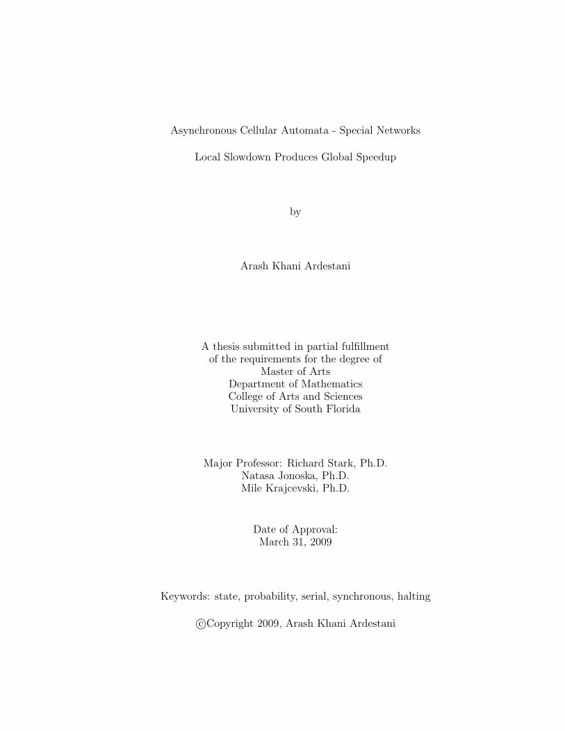
We can compute the average halting time for the 2PartitioN square network with
serial activity. To do so we need to formulate the expected halting time in relation to
the transition probability and the probability of activity for a given initial state:
Hα = 1 +∑
PµHµ
• Hα the expected halting time from the state α for example H0011
• µ the state to which we have a single step transition from state α
• Hµ the expected halting time for the state µ for example H0111
• Pµ the probability that state µ will have one step transition from state α.
Note: In this case Pµ = 1/4 for all µ. As an example let us write a formula for calculating
the expected halting time for state α = 0011:
H0011 = 1 + [1/4(H1011) + 1/4(H0111) + 1/4(H0001) + 1/4(H0010)]
To find the average expected halting time we will follow these simple steps:
Step 1: Using global state transition diagram find the expected halting time for each
initial state in terms of other
Step 2: Write the equation for each expected halting time in terms of each initial state
and other states
Step 3: Set these equations as a system with 16 equations and 14 unknowns 3 and solve
it using Maple
Step 4: Find the average of the expected halting times
Let us begin with step 1:
H0011 = 1 + [1/4(H1011) + 1/4(H0111) + 1/4(H0001) + 1/4(H0010)]
H1011 = 1 + [1/4(H0011) + 1/4(H1010) + 1/4(H1001) + 1/4(H1011)]
H1111 = 1 + [1/4(H0111) + 1/4(H1011) + 1/4(H1101) + 1/4(H1110)]
H1001 = 0
3There are only 14 unknowns because H0110 and H1001 are zero
15

H1010 = 1 + [1/4(H0010) + 1/4(H1110) + 1/4(H1000) + 1/4(H1011)]
H1101 = 1 + [1/4(H0101) + 1/4(H1100) + 1/4(H1001) + 1/4(H1101)]
H1110 = 1 + [1/4(H1100) + 1/4(H1010) + 1/4(H0110) + 1/4(H1110)]
H1000 = 1 + [1/4(H1100) + 1/4(H1010) + 1/4(H1001) + 1/4(H1000)]
H1100 = 1 + [1/4(H0100) + 1/4(H1000) + 1/4(H1110) + 1/4(H1101)]
H0111 = 1 + [1/4(H0011) + 1/4(H0101) + 1/4(H0110) + 1/4(H0111)]
H0101 = 1 + [1/4(H1101) + 1/4(H0001) + 1/4(H0111) + 1/4(H0100)]
H0110 = 0
H0100 = 1 + [1/4(H1100) + 1/4(H0110) + 1/4(H0101) + 1/4(H0100)]
H0001 = 1 + [1/4(H1001) + 1/4(H0101) + 1/4(H0011) + 1/4(H0001)]
H0000 = 1 + [1/4(H1000) + 1/4(H0100) + 1/4(H0010) + 1/4(H0001)]
H0010 = 1 + [1/4(H1010) + 1/4(H0110) + 1/4(H0011) + 1/4(H0010)]
After solving the system of equations using Maple, the following values are obtained:
H0011 = 7.062499992 H1011 = 6.083333325
H1111 = 7.166666657 H1001 = 0.0
H1010 = 7.187499990 H1101 = 6.083333325
H1110 = 6.458333325 H1000 = 6.124999992
H1100 = 7.187499992 H0111 = 6.041666658
H0101 = 7.062499988 H0110 = 0.0
H0100 = 6.083333325 H0001 = 6.041666658
H0000 = 7.083333323 H0010 = 6.083333325 .
The average expected halting time is 6.553571419
As mentioned earlier the basic property of a serial network is apparent in the way the cell
activity takes place. For the purpose of 2PartitioN square network with serial activity,
only one of the four cells can be active at a time. There is an inevitable need for a
mechanism to ensure that no more than one cell can be active at a given time. There
are different methods to implement this mechanism. One mechanism would be using a
16

clock just like the clock mentioned in the 2Partition square network with synchronous
activity. Another mechanism would be to use a token, similar to the technology used in
token ring networks. Depending on the size and structure of the network one mechanism
may be preferred over another, but that subject is out of the scope of this article. In any
event enforcing serial activity on this model requires a substantial computational effort.
The ideal goal with 2PartitioN network -cellular network of automata- is to be able to
design the cells in such a way that the memory requirement is minimal to none and that
they are programmed in the simplest way possible. In the next section we will describe
a special kind of 2PartitioN network that is the closest to the ideal model.
17

5 2PartitioN program on a square network with asyn-
chronous activity
Considering the same 2PartitioN network that we have been analyzing so far, but
the major different this time is that we allow any of the cells to be active at any given time.
Even though this change in the cells’ activity may seem minor at first, yet deeper analysis
of the network proves that the impact on the network’s behavior and more importantly
its halt-ability is absolutely significant. We introduce this network as 2PartitioN square
asynchronous. The word asynchronous here is meant to describe the randomness in each
cell’s activity. At first glance it might appear as if the asynchronous network design
will be more complex but it turns out that the asynchronous network does not need a
clock and each cell is designed with a much simpler program, compared to the networks
examined in the previous sections. A major difference between the 2PartitioN network
with asynchronous activity and the 2PartitioN network with synchronous activity is that
the first one will always halt, while the latter may or may not halt.
It is interesting to notice that the state transition of the 2PartitioN square network
with serial and synchronous activity are both special cases of the 2PartitioN square
network with Asynchronous activity. This also means that the global state diagrams
of the 2PatitioN square network with serial and synchronous activity are subsets of the
global state diagram for the 2PartitioN square network with asynchronous activity. In
2PartitioN square asynchronous network we relax the rules that govern the activity of
the cells; thus giving the network more flexibility and perhaps more complexity.
Before going further let us demonstrate a figure to familiarize ourselves with how this
network behaves.
18

Figure 12: state transitions of 2PartitioN asynchronous network.
Obviously this process continues until it reaches any of the two halting states. As
mentioned earlier the 2PartitioN square network is a halting network. It is important to
mention that 2Partition must halt on bipartite graphs.
Theorem: 2PartitioN on square network in asynchronous mode will always halt.
Proof:
Suppose we are at one of the random initial states. The greatest probability that the
next state is not one of the halting states is at most P where P < 1. Suppose we go
to the next non-halting state and again the probability of going to the next non-halting
state is ≤ P . If we continue in this fashion for n steps, then the probability that we do
not reach a halting state in n steps is ≤ P n. On the other hand the probability that the
network halts in n steps is ≤ 1 − P n. As n goes to ∞ then P n approaches 0 therefore
1− P n approaches 1.
limn→∞ (P n) = 0 ⇒ limn→∞ (1− P n) = 1 �
This shows that 2PartitioN on square network in asynchronous mode will always halt
with probability 1. To make this point clearer let’s demonstrate the case below:
19

Figure 13: Example of state transition and values for P.
.
In the figure on the left the P is calculated as P = (1 − 1/8) = 7/8 where in the right
figure we have P = 1− 1 = 0.
Figure below represents the global state diagram of the 2PartitioN square asynchronous
network:
20

Figure 14: Global state diagram - 2PartitioN square asynchronous Network.
.
To demonstrate this more clearly let’s present the next figure:
21

Figure 15: Partial global state diagram - 2PartitioN square asynchronous Network.
.
The figure above captures a potion of the previous diagram and demonstrates how each
initial state is related to other states including the halting states. Clearly not all the
states are shown, due to lack of space to include all arrows and all states, but the
figure delivers the point. Perhaps, the next few paragraphs explain the dynamics of the
network better. To obtain the next states from each initial state, we consider all possible
22

combinations of active cells a, b, c, and d, skipping the repetitions of course. In general
we will consider the following 16 cases:
None of the cells are active
Case 1: No cell is active
Just single cell being active
Case 2: Only cell ”a” is active
Case 3: Only cell ”b” is active
Case 4: ....
............
All combinations of two cells being active at a time
Case 6: Cells ”a” and ”b” are active
Case 7: Cells ”a” and ”c” are active
Case 8: ....
............
............
All combinations of three cells being active at a time
Case 12: Cells ”a” and ”b” and ”c” are active
Case 13: Cells ”a” and ”b” and ”d” are active
All four cells active at a time
Case 16: Cells ”a” and ”b” and ”c” and ”d” are active
Mathematically we are basically taking all the subsets of the set of cells C = {a, b, c, d}to obtain the set of active cells. In each case the members of each subset define the active
cells for that case.
Let us examine one of initial random states and see how it would go to all other
possible states:
23

Figure 16: State transition from state A to all other possible states.
.
Now that we have seen this construction one can easily see the relation between each
initial state and the next possible states demonstrated in figure-16. One can quickly
notice that some of the initial random states can only change to eight of the sixteen
possible next states. The reason behind this configuration is that in some of the random
initial states one of the cells is what we call a stable cell. A stable cell is cell that does not
have any neighbor with the same value as itself; thus it has no effect on the computation
of the next state. According to the transition function defined in Section 1, the stable
cell does not need to change its value regardless if it is active or not -alone or in any
combination with other cells- Let us demonstrate this behavior in the following figure,
where cell ”b” is the stable cell:
24

Figure 17: State transition when there is a free cell.
.
So far we have established the fact that the 2ParitioN square network with asynchronous
activity will always halt. Additionally we have determined a complete global transition
graph, which shows the relation between every possible random initial state and all the
other states, including the halting states. Now it would be interesting to examine each
random initial state to see how the activity of each cell can affect the next transition
state. To study and analyze this process we will take advantage of the notion of transition
probability. What we mean by transition probability is the probability that a given
random initial state would go to the next possible state. We will study the relation
between the probability of activity (for each cell in a given random initial state) and the
transition probability. Let us begin with the following example:
Figure 18: Example 1 of how transition probabilities are computed.
25

.
For each active cell we assign the value p and for each inactive cell we assign the value
(1 - p). If there is a stable cell, the process is the same, but the total probabilities will
be added together just like in the following example:
Figure 19: Example 2 of how transition probabilities are computed.
.
In example 1 to compute the total probabilities going from 1010 to 1110 we have:
P1010→1110 = (1− p)3(p)
In example 2 to compute the total probabilities going from 0111 to 0110 we have:
P0111→0110 = (1− p)3(p) + (1− p)2(p)2
By design, we let each cell in the square network with asynchronous activity to be active
or inactive at any given time. Therefore the probability of a cell being active is p = 1/2.
Similarly the probability of a cell being inactive is also 1/2 (i.e. 1 - p = 1/2). There
are four cells in the square network, so the total probability for going from one state to
another is calculated as 1/16. Of course in some of the states where we have stable cells,
the probability would be 2P = 1/8.
As seen in figure-17 each random initial state will end on at least one of the halting
states. This is visual confirmation of the proof of Theorem-1. The fact that this network
is a halting network brings up a few interesting questions:
26

• What is the expected halting time of the 2PartitioN asynchronous network?
• Does the choice of initial state affect the average expected halting time?
To answer these question we will use the same method as we used in Section 3 pages 13-14:
Hα = 1 +∑
PµHµ
• Hα the expected halting time from the state α for example H0011
• µ the state from which we have a single step transition from state α
• Hµ the expected halting time for the state µ for example H0111
• Pµ the probability that state µ will be obtained in one step transition from state
α.
It is important to note that in the current case Pµ = 1/16 for all µ. So if we were to
write a formula for calculating the expected halting time for state α = 0011 we would
have:
H0011 = 1 + [1/16(H0011) + 1/16(H1011) + 1/16(H1111) + 1/16(H1001) + 1/16(H1010)
+1/16(H1101) + 1/16(H1110) + 1/16(H1000) + 1/16(H1100) + 1/16(H0111) + 1/16(H0101)
+1/16(H1001) + 1/16(H0100) + 1/16(H0001) + 1/16(H0000) + 1/16(H0010)]
Using the global state diagram and the activity probability P for each state we can
write the equations of halting for each of the random initial state as follows:
H0011 = 1 + 1/16[H0011 +H1011 +H1111 +H1001 +H1010 +H1101 +H1110+
H1000 +H1100 +H0111 +H0101 +H0110 +H0100 +H0001 +H0000 +H0010]
H1011 = 1 + 1/16[2H0011 + 2H1011 + 2H0001 + 2H1000 + 2H1010 + 2H1001 + 2H0010 + 2H0000]
27

H1111 = 1 + 1/16[H0011 +H1011 +H1111 +H1001 +H1010 +H1101 +H1110+
H1000 +H1100 +H0111 +H0101 +H0110 +H0100 +H0001 +H0000 +H0010]
H1001 = 0
H1010 = 1 + 1/16[H0011 +H1011 +H1111 +H1001 +H1010 +H1101 +H1110+
H1000 +H1100 +H0111 +H0101 +H0110 +H0100 +H0001 +H0000 +H0010]
H1101 = 1 + 1/16[2H1101 + 2H0101 + 2H0001 + 2H0100 + 2H0000 + 2H1001 + 2H1000 + 2H1100]
H1110 = 1 + 1/16[2H1110 + 2H0110 + 2H0010 + 2H0100 + 2H0000 + 2H1010 + 2H1000 + 2H1100]
H1000 = 1 + 1/16[2H1000 + 2H1100 + 2H1010 + 2H1001 + 2H1110 + 2H1101 + 2H1111 + 2H1011]
H1100 = 1 + 1/16[H0011 +H1011 +H1111 +H1001 +H1010 +H1101 +H1110+
H1000 +H1100 +H0111 +H0101 +H1001 +H0100 +H0001 +H0000 +H0010]
H0111 = 1 + 1/16[2H0111 + 2H0011 + 2H0101 + 2H0110 + 2H0001 + 2H0010 + 2H0100 + 2H0000]
H0101 = 1 + 1/16[H0011 +H1011 +H1111 +H1001 +H1010 +H1101 +H1110+
H1000 +H1100 +H0111 +H0101 +H1001 +H0100 +H0001 +H0000 +H0010]
H1001 = 0
H0100 = 1 + 1/16[2H0100 + 2H1100 + 2H1110 + 2H1101 + 2H1111 + 2H0110 + 2H0101 + 2H0111]
H0001 = 1 + 1/16[2H0001 + 2H1001 + 2H1101 + 2H1011 + 2H1111 + 2H0101 + 2H0111 + 2H0011]
H0000 = 1 + 1/16[H0011 +H1011 +H1111 +H1001 +H1010 +H1101 +H1110+
28

H1000 +H1100 +H0111 +H0101 +H1001 +H0100 +H0001 +H0000 +H0010]
H0010 = 1 + 1/16[2H0010 + 2H1010 + 2H1110 + 2H1011 + 2H1111 + 2H0110 + 2H0111 + 2H0011]
We consider this as a system of equations with 14 unknowns 4 where Hx interprets
as the expected halting time for state x. Solving this system of equations will result in
a numerical value for the expected halting time for each of 16 possible states.
H0011 = 8.031249990 H1011 = 8.028124995
H1111 = 8.093749991 H1001 = 0.0
H1010 = 8.031249986 H1101 = 8.028124997
H1110 = 8.028124997 H1000 = 8.034374998
H1100 = 8.031249992 H0111 = 8.028124996
H0101 = 8.031249992 H0110 = 0.0
H0100 = 8.034374996 H0001 = 8.034374991
H0000 = 8.031249992 H0010 = 8.034374998 .
The average expected halting time is easily calculated to be 8.035714279
Clearly changing the probability of activity for each cell will change the transition prob-
ability. This brings up a few more interesting questions:
• How will changing cell activity probability affect the transition probability?
• Will changing the transition probability affect the expected halting time?
• How will the change in transition probability affect the expected halting time?
To answer these questions we write the halting equation for each of the random initial
states leaving the cell activity probability as a variable p. To find the minimum halting
time we differentiate the equation again with p staying as a variable. The idea is to write
generic equations based on the formula bottom of page 22 and equations shown on pages
4There are only 14 unknowns because H0110 and H1001 are zero
29

23 - 24, except that not the probability of activity for each cell is left as variable p. To
deliver a clearer point let’s look at the following example: Support we are at the random
initial state [0011] and we want to compute the expected halting. The base formula is:
Hα = 1 +∑
PµHµ
So in this case α is 0011. To find the pµ we will refer to the global state diagram to
see how 0011 will change to other states and find those transition probabilities based on
probability of activity:
30
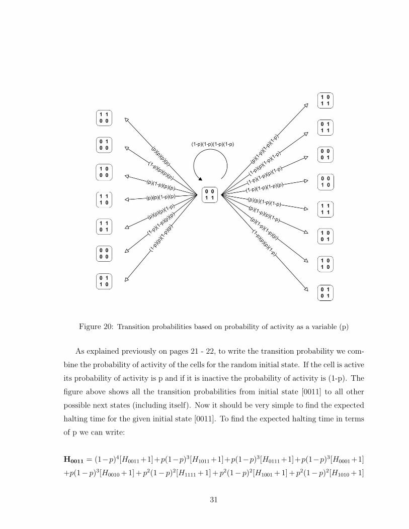
Figure 20: Transition probabilities based on probability of activity as a variable (p)
As explained previously on pages 21 - 22, to write the transition probability we com-
bine the probability of activity of the cells for the random initial state. If the cell is active
its probability of activity is p and if it is inactive the probability of activity is (1-p). The
figure above shows all the transition probabilities from initial state [0011] to all other
possible next states (including itself). Now it should be very simple to find the expected
halting time for the given initial state [0011]. To find the expected halting time in terms
of p we can write:
H0011 = (1−p)4[H0011 +1]+p(1−p)3[H1011 +1]+p(1−p)3[H0111 +1]+p(1−p)3[H0001 +1]
+p(1− p)3[H0010 + 1] + p2(1− p)2[H1111 + 1] + p2(1− p)2[H1001 + 1] + p2(1− p)2[H1010 + 1]
31

+p2(1− p)2[H0101 + 1] + p2(1− p)2[H0110 + 1] + p2(1− p)2[H0000 + 1] + p3(1− p)[H1101 + 1]
+p3(1− p)[H1110 + 1] + p3(1− p)[H1000 + 1] + p3(1− p)[H0100 + 1] + p4[H1100 + 1]
32

.
Let us demonstrate this point with another figure and example, where now the initial
state has a stable cell:
Figure 21: Transition probabilities for an initial state with stable cell
.
similarly to find the expected halting time in terms of (p) for initial state [1101] we have:
H1101 = [(1− p)4 + p(1− p)3][H1101 + 1] + [p(1− p)3 + p2(1− p)2][H0101 + 1]
+[p(1− p)3 + p2(1− p)2][H1001 + 1] + [p(1− p)3 + p2(1− p)2] + [H1100 + 1]
+[p2(1− p)2 + p3(1− p)][H0001 + 1] + [p2(1− p)2 + p3(1− p)][H0100 + 1]
+[p2(1− p)2 + p3(1− p)][H1000 + 1] + [p3(1− p) + p4][H0000 + 1]
Now we can write similar equations corresponding to each of the 16 initial states and
33
find the expected halting time for each initial state in terms of p as a variable. We can
then set these equations as a system with 16 unknowns. Once the equation is solved
we will be left with one final equation in terms of p as a variable. Clearly we can find
the minimum value for that equation by differentiating with respect to p and finding the
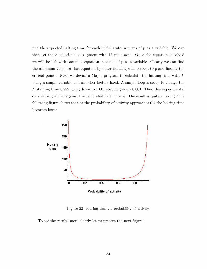
critical points. Next we devise a Maple program to calculate the halting time with P
being a simple variable and all other factors fixed. A simple loop is setup to change the
P starting from 0.999 going down to 0.001 stepping every 0.001. Then this experimental
data set is graphed against the calculated halting time. The result is quite amazing. The
following figure shows that as the probability of activity approaches 0.4 the halting time
becomes lower.
Figure 22: Halting time vs. probability of activity.
To see the results more clearly let us present the next figure:
34

Figure 23: Close up of halting time vs. probability of activity.
By solving the equations we find that at P = 0.406 the halting time is the lowest
halting time for the 2PartitioN square asynchronous network being precisely at 7.5838286.
Interestingly enough this halting time is certainly lower than the one we calculated using
the 16 equations explored earlier. In addition this lower halting time was achieved using
a lower probability of activity than P = 1/2. It is also important to note that when the
probability of activity for the cells is close to 1, meaning each cell is active at all times,
the halting time approaches infinity. In other word, it will take this network forever to
halt.
35
6 Philosophy and conclusion
The results obtained in previous section are not what we would expect. Imagine with
this network was a simple computer with four processors, trying to solve a problem. In
reality by increasing the activity of each processor one would expect to solve the problem
faster, but in this case we realized that slowing down each processor just enough, would
make the simple computer solve the problem faster. Let us consider a scenario where
we have finitely many of these 2PartitioN square asynchronous networks in a large grid.
Each 2PartitioN square network has four links to four other 2PartitioN network. All the
squares are at rest in a random initial state. Randomly we activate one of the 2PartitioN
square networks. As soon as this one network reaches the halting state, it activates its four
links to other four neighboring networks. Then each of those four neighboring networks
become active and begin to work their way towards halting. This process continues for
a finite period of time, until all the 2PartitioN squares are halted in the entire grid.
This process very much simulates the healing process of an organ or tissue in a living
organism. Suppose each 2PartitioN square network in this grid is setup with a probability
of activity as P = 1/2. Then we can easily predict the average time for given number
of cells to reach their goal, in this case healing of the entire tissue. Obviously if there is
a special substance that can lower the probability of activity in each cell, thus slowing
down the 2PartitioN square networks to the desired level –remember the P = 0.406– then
we can certainly achieve a significantly faster healing process when working with large
tissues consisting of millions of cells. So far quite a few mathematicians have attempted
to provide the closest and most ideal mathematical model to cell interaction and growth
as seen in nature. The approach to this mathematical model may seem simple; however
it provides a bridge between traditional computation models and new approaches to
understanding cellular networks in nature. We have all observed the usual computation
models in any regular computing machine, anything from a simple Turing machine to
a fast super computer. The idea has always been to use highly regular and organized
models with strict set of rules governing the model and its elements. Today’s science
36

however demands one to break free of regularity and order, to look at a model seemingly
overwhelmed in chaos, but with just enough order to represent a sophisticated model of
cellular activity in nature.
37

References
.
Brzozowski, J.A. and R. Negulescu, Automata of Asynchronous Behav-
iors, Theoretical Computer Science, Vol. 231, Issue 1, pp. 113-128, 17 January 2000.
Dijkstra, Self-stabilizing systems in spite of distributed control, CACM pp.643-645,
n. 11, v. 17, 1974.
H. Bersini and V. Detours, 1994. Asynchrony induces stability in cellular
automata based models, Proceedings of the IVth Conference on Artificial Life , pages
382-387, Cambridge, MA, July 1994, vol 204, no. 1-2, pp. 70-82.
Nehaniv, C. L. 2004 Asynchronous Automata Networks Can Emulate Any Syn-
chronous Automata Network, International Journal of Algebra and Computation, 14(5-
6):719-739.
Stark W.R. Asynchronous Networks of Automata - A Study of Emergent Phonom-
ena from Mathematical Analysis to Biologically Inspired Applications, Department of
Mathematics and Statistics - University of South Florida, Tampa Florida
Strogatz, Steven, 2003, SYNC, The emerging Science of Spontaneous Order, 1st
Edition, New York
von Neumann, John, 1966, The Theory of Self-reproducing Automata, A. Burks,
ed., Univ. of Illinois Press, Urbana, IL.
38

Appendix A
39

40

41

42

43

44

45

46

47


![A cellular learning automata based algorithm for detecting ... · by combining cellular automata (CA) and learning automata (LA) [22]. Cellular learning automata can be defined as](https://img.pdfslide.us/doc/110x75/601a3ee3c68e6b5bec07f1bb/a-cellular-learning-automata-based-algorithm-for-detecting-by-combining-cellular.jpg)

![Understanding Organism Growth and Cellular Differentiation ......cellular automata (see [44][17] for brief surveys). Cellular automata as described by Von Neumann Cellular automata](https://img.pdfslide.us/doc/110x75/60b713ba0a03b236086940aa/understanding-organism-growth-and-cellular-diierentiation-cellular-automata.jpg)