Asymptotics oforthogonal polynomials in normal

matrix ensemble

Seung-Yeop Lee (University of South Florida)

Cincinnati, September 20th 2014

1 / 32

Joint work with Roman Riser.

Many discussions with Marco Bertola, Robert Buckingham,Maurice Duits, Kenneth McLaughlin, ...

2 / 32

Main actors:

I Orthogonal polynomials

I Two dimensional Coulomb gas

I Hele-Shaw flow

3 / 32

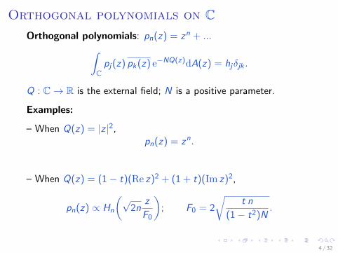
Orthogonal polynomials on COrthogonal polynomials: pn(z) = zn + ...∫

Cpj(z) pk(z) e−NQ(z)dA(z) = hjδjk .

Q : C→ R is the external field; N is a positive parameter.

Examples:

– When Q(z) = |z |2,pn(z) = zn.

– When Q(z) = (1− t)(Re z)2 + (1 + t)(Im z)2,

pn(z) ∝ Hn

(√2n

z

F0

); F0 = 2

√t n

(1− t2)N.

4 / 32

2D Coulomb gas (Eigenvalues)

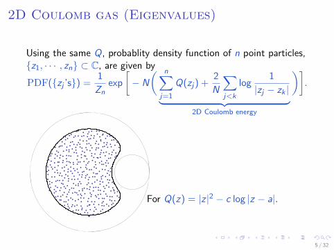
Using the same Q, probablity density function of n point particles,{z1, · · · , zn} ⊂ C, are given by

PDF({zj ’s}) =1

Znexp

[− N

( n∑j=1

Q(zj) +2

N

∑j<k

log1

|zj − zk |︸ ︷︷ ︸2D Coulomb energy

)].

For Q(z) = |z |2 − c log |z − a|.

5 / 32

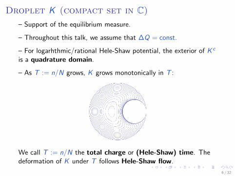
Droplet K (compact set in C)– Support of the equilibrium measure.

– Throughout this talk, we assume that ∆Q = const.

– For logarhthmic/rational Hele-Shaw potential, the exterior of K c

is a quadrature domain.

– As T := n/N grows, K grows monotonically in T :

We call T := n/N the total charge or (Hele-Shaw) time. Thedeformation of K under T follows Hele-Shaw flow.

6 / 32

Exterior conformal map of K

For simplicity, we assume that K is simply connected so that wecan define the unique riemann mapping

f : K c → Dc

such that

f (z) =z

ρ+O(1), ρ > 0, as |z | → ∞.

Geometry of K is encoded in f .

For example, the curvature of the boundary of K is given by

κ = Re

(1− f ′′f

(f ′)2

)|f ′|

where the prime ′ stands for the complex derivative.

7 / 32

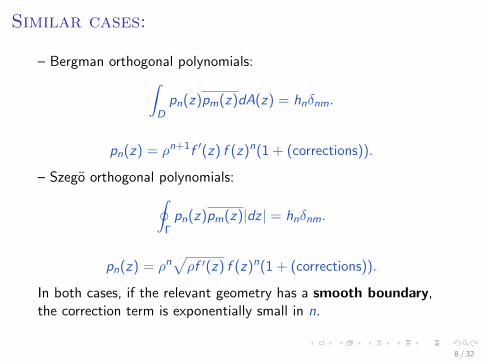
Similar cases:

– Bergman orthogonal polynomials:∫Dpn(z)pm(z)dA(z) = hnδnm.

pn(z) = ρn+1f ′(z) f (z)n(1 + (corrections)).

– Szego orthogonal polynomials:∮Γpn(z)pm(z)|dz | = hnδnm.

pn(z) = ρn√ρf ′(z) f (z)n(1 + (corrections)).

In both cases, if the relevant geometry has a smooth boundary,the correction term is exponentially small in n.

8 / 32

Conjecture

(If the potential Q is such that K has real analytic boundary,) thestrong asymptotics of pn(z) as n→∞ and N →∞ whileT := n/N is finite, is given by

pn(z) =√ρf ′(z) eng(z)

(1 +

1

NΨ(z) +O

(1

N2

)), z /∈ K .

The function g (called g -function) is the complex logarithmicpotential generated by the measure 1K :

g(z) =1

πT

∫K

log(z − ζ)dA(ζ).

The function Ψ is in the next page.

9 / 32

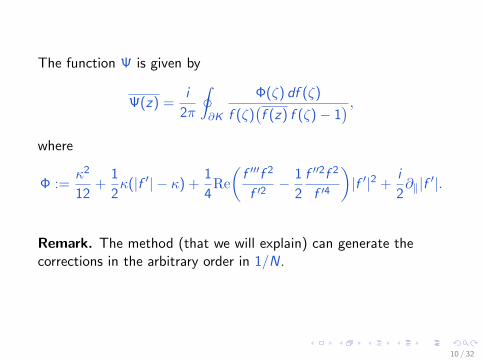
The function Ψ is given by

Ψ(z) =i

2π

∮∂K

Φ(ζ) df (ζ)

f (ζ)(f (z) f (ζ)− 1

) ,where

Φ :=κ2

12+

1

2κ(|f ′| − κ) +

1

4Re

(f ′′′f 2

f ′2− 1

2

f ′′2f 2

f ′4

)|f ′|2 +

i

2∂‖|f ′|.

Remark. The method (that we will explain) can generate thecorrections in the arbitrary order in 1/N.

10 / 32

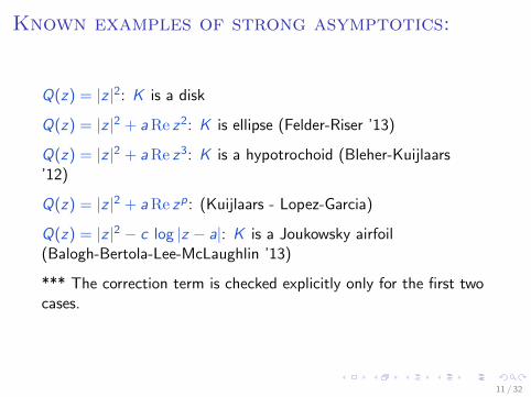
Known examples of strong asymptotics:

Q(z) = |z |2: K is a disk

Q(z) = |z |2 + aRe z2: K is ellipse (Felder-Riser ’13)

Q(z) = |z |2 + aRe z3: K is a hypotrochoid (Bleher-Kuijlaars’12)

Q(z) = |z |2 + aRe zp: (Kuijlaars - Lopez-Garcia)

Q(z) = |z |2 − c log |z − a|: K is a Joukowsky airfoil(Balogh-Bertola-Lee-McLaughlin ’13)

*** The correction term is checked explicitly only for the first twocases.

11 / 32

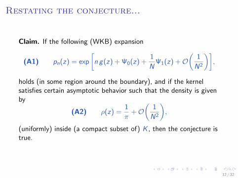
Restating the conjecture...

Claim. If the following (WKB) expansion

(A1) pn(z) = exp

[n g(z) + Ψ0(z) +

1

NΨ1(z) +O

(1

N2

)],

holds (in some region around the boundary), and if the kernelsatisfies certain asymptotic behavior such that the density is givenby

(A2) ρ(z) =1

π+O

(1

N2

),

(uniformly) inside (a compact subset of) K , then the conjecture istrue.

12 / 32

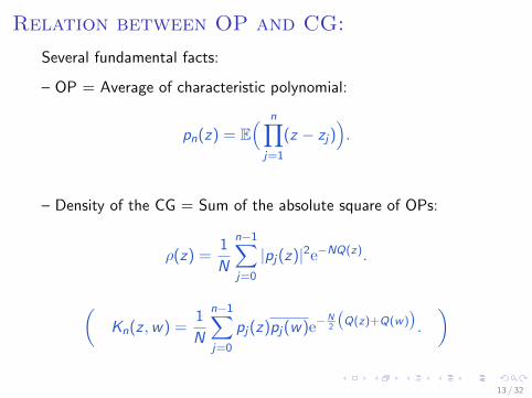
Relation between OP and CG:

Several fundamental facts:

– OP = Average of characteristic polynomial:

pn(z) = E( n∏

j=1

(z − zj)).

– Density of the CG = Sum of the absolute square of OPs:

ρ(z) =1

N

n−1∑j=0

|pj(z)|2e−NQ(z).

(Kn(z ,w) =

1

N

n−1∑j=0

pj(z)pj(w)e−N2

(Q(z)+Q(w)

).

)

13 / 32

Hele-Shaw potential

The density of the Coulomb gas is given by

ρ(z) :=

∫PDF(z , z2, · · · , zn)

n∏j=2

dA(zj)→∆Q

4πwhen z ∈ K .

Q(z) = |z |2 Q(z) = |z |2 − tRe(z2)

14 / 32

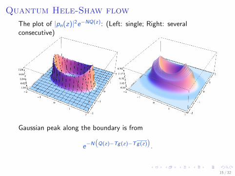
Quantum Hele-Shaw flow

The plot of |pn(z)|2e−NQ(z): (Left: single; Right: severalconsecutive)

Gaussian peak along the boundary is from

e−N(Q(z)−Tg(z)−Tg(z)

).

15 / 32

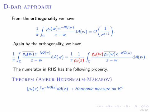
D-bar approach

From the orthogonality we have

1

π

∫C

pn(w) e−NQ(w)

z − wdA(w) = O

(1

zn+1

).

Again by the orthogonality, we have

1

π

∫C

pn(w) e−NQ(w)

z − wdA(w) =

1

π

1

pn(z)

∫C

pn(w) pn(w) e−NQ(w)

z − wdA(w).

The numerator in RHS has the following property.

Theorem (Ameur-Hedenmalm-Makarov)

|pn(z)|2e−NQ(z)dA(z)→ Harmonic measure on K c

16 / 32

1/N-expansion of Cauchy transformFor a smooth test function f ,∫

Cf (ζ) e−N

(Q(ζ)−g(ζ)−g(ζ)+`

)dA(ζ)

=

√π

2N

∮∂K

(f (ζ) +

1

N

(κ2

12f (ζ) +

3κ

8∂nf (ζ) +

1

8∂2

nf (ζ)

)+O

(1

N2

))|dζ|.

(This is obtained by using Schwarz function.)

We take

f (ζ) =|pn(ζ)|2

ζ − z

where pn is all the subleading parts of pn:

pn(z) := pn(z) e−ng(z) = eΨ0

(1 +

1

NΨ1 +O

(1

N2

)).

17 / 32

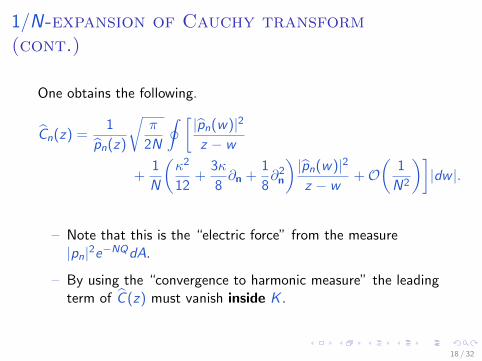
1/N-expansion of Cauchy transform(cont.)

One obtains the following.

Cn(z) =1

pn(z)

√π

2N

∮ [|pn(w)|2

z − w

+1

N

(κ2

12+

3κ

8∂n +

1

8∂2

n

)|pn(w)|2

z − w+O

(1

N2

)]|dw |.

– Note that this is the “electric force” from the measure|pn|2e−NQdA.

– By using the “convergence to harmonic measure” the leadingterm of C (z) must vanish inside K .

18 / 32

Therefore, in the leading order,

|pn(w)|2 ≈ |e2Ψ0 | ∝ |f ′|.

And this leads toeΨ0(z) =

√ρf ′(z).

(This is not the main point.)

To calculate the next order, we claim that Cn vanishes even at thesecond order. This is not proven in general, however it follows fromcertain asymptotics of the kernel (which is also not proven ingeneral).

19 / 32

Kernel → Cauchy transform

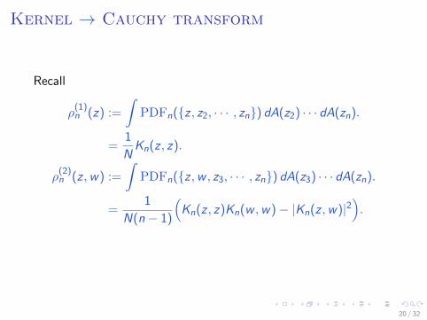
Recall

ρ(1)n (z) :=

∫PDFn({z , z2, · · · , zn}) dA(z2) · · · dA(zn).

=1

NKn(z , z).

ρ(2)n (z ,w) :=

∫PDFn({z ,w , z3, · · · , zn}) dA(z3) · · · dA(zn).

=1

N(n − 1)

(Kn(z , z)Kn(w ,w)− |Kn(z ,w)|2

).

20 / 32

Taking ∂z on the first equation:

∂ρ(1)n (z) =

∫ (− NQ ′(z) +

n∑j=2

1

z − zj

)ρn({z , z2, · · · , zn})

n∏j=2

dA(zj)

= −NQ ′(z)ρ(1)n (z) + (n − 1)

∫dA(w)

z − wρ

(2)n ({z ,w , z3, · · · , zn})

n∏j=3

dA(zj)

= −NQ ′(z)ρ(1)n (z) +

1

N

∫dA(w)

z − w

(Kn(z , z)Kn(w ,w)− |Kn(z ,w)|2

).

Divide the whole equation by ρ(1)n (z) = 1

NKn(z , z). Obtain the

same equation for ρ(1)n+1 and take the difference of the two.

We obtain∫|pn(w)|2e−NQ(w)dA(w)

z − w=

1

Kn(z , z)

∫|Kn(z ,w)|2dA(w)

z − w

+(terms with ∂ρ(1)n (z))

21 / 32

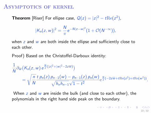
Asymptotics of kernel

Theorem [Riser] For ellipse case, Q(z) = |z |2 − tRe(z2),

|Kn(z ,w)|2 =N

πe−N|z−w |

2(1 +O(N−∞)),

when z and w are both inside the ellipse and sufficiently close toeach other.

Proof) Based on the Christoffel-Darboux identity:

1

N∂w(Kn(z ,w) e

N2

(|z|2+|w |2−2zw))

=

√n

N

t pn(z) pn−1(w)− pn−1(z) pn(w)√hnhn−1

√1− t2

eN2

(−2zw+tRe(z2)+tRe(w2)).

When z and w are inside the bulk (and close to each other), thepolynomials in the right hand side peak on the boundary.

22 / 32

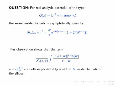
QUESTION: For real analytic potential of the type:

Q(z) = |z |2 + (harmonic)

the kernel inside the bulk is asymptotically given by

|Kn(z ,w)|2 =N

πe−N|z−w |

2(1 +O(N−∞)).

This observation shows that the term

1

Kn(z , z)

∫|Kn(z ,w)|2dA(w)

z − w

and ∂ρ(1)n are both exponentially small in N inside the bulk of

the ellipse.

23 / 32

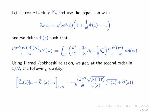
Let us come back to Cn and use the expansion with:

pn(z) =√ρψ′(z)

(1 +

1

NΨ(z) + ...

)and we define Φ(z) such that

ρ|ψ′(w)|Φ(w)

z − wdA(w) :=

∮∂K

(κ2

12+

3κ

8∂n +

1

8∂2

n

)ρ|ψ′(w)|z − w

dA(w).

Using Plemelj-Sokhotski relation, we get, at the second order in1/N, the following identity:[

Cn(z)|in − Cn(z)|out

]1/N

= −√

2π3

N

√ρψ′(z)

ψ(z)

(Ψ(z) + Φ(z)

).

24 / 32

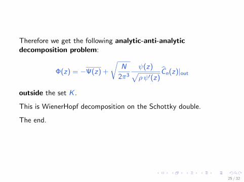
Therefore we get the following analytic-anti-analyticdecomposition problem:

Φ(z) = −Ψ(z) +

√N

2π3

ψ(z)√ρψ′(z)

Cn(z)|out

outside the set K .

This is WienerHopf decomposition on the Schottky double.

The end.

25 / 32

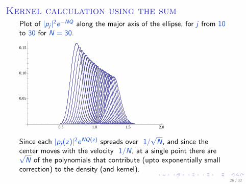
Kernel calculation using the sum

Plot of |pj |2e−NQ along the major axis of the ellipse, for j from 10to 30 for N = 30.

0.5 1.0 1.5 2.0

0.05

0.10

0.15

Since each |pj(z)|2eNQ(z) spreads over 1/√N, and since the

center moves with the velocity 1/N, at a single point there are√N of the polynomials that contribute (upto exponentially small

correction) to the density (and kernel).

26 / 32

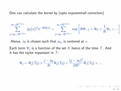
One can calculate the kernel by (upto exponentiall correction)

n0+N1/2+ε∑j=n0−N1/2+ε

|pj(z)|2e−NQ(z) =

n0+N1/2+ε∑j=n0−N1/2+ε

exp

[NΨ−1 + Ψ0 +

1

NΨ1 + ...

]

Above, n0 is chosen such that pn0 is centered at z .

Each term Ψj is a function of the set K hence of the time T . Andit has the taylor expansion in T :

Ψj = Ψj(T0) +j − n0

NΨj(T0) +

(j − n0)2

2N2Ψj(T0) + ...

27 / 32

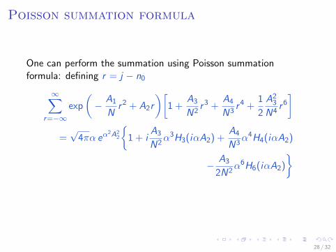
Poisson summation formula

One can perform the summation using Poisson summationformula: defining r = j − n0

∞∑r=−∞

exp

(− A1

Nr2 + A2r

)[1 +

A3

N2r3 +

A4

N3r4 +

1

2

A23

N4r6

]=√

4πα eα2A2

2

{1 + i

A3

N2α3H3(iαA2) +

A4

N3α4H4(iαA2)

− A3

2N2α6H6(iαA2)

}

28 / 32

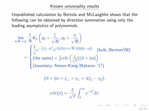
Known universality results

Unpublished calculation by Bertola and McLaughlin shows that thefollowing can be obtained by direction summation using only theleading asymptotics of polynomials.

limn,N→∞

1

NKn

(z0 +

ξ√N, z0 +

η√N

)

=

1

πe−

12|ξ−η|2ei=(ξη)+i

√N =(z0(ξ−η)) (bulk,Berman′08)

(the same)× 12erfc

(1√2

(ξn + ηn))

(boundary, Ameur-Kang-Makarov ’1?)

ξn + ηn = ξ⊥ + η⊥ + i(ξ‖ − η‖).

erfc(z) =2√π

∫ ∞z

e−t2dt.

29 / 32

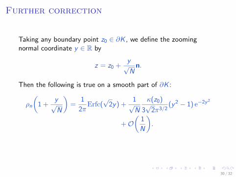
Further correction

Taking any boundary point z0 ∈ ∂K , we define the zoomingnormal coordinate y ∈ R by

z = z0 +y√N

n.

Then the following is true on a smooth part of ∂K :

ρn

(1 +

y√N

)=

1

2πErfc(

√2y) +

1√N

κ(z0)

3√

2π3/2(y2 − 1) e−2y2

+O(

1

N

).

30 / 32

From kernel to orthogonal polynomial

If we use the second assumption (A2) then the correction terms ofthe density in each order or 1/N must vanish. Using Poissonsummation formula, this gives another recursive method to obtainhigher order corrections of OP (work in progress with RomanRiser).

31 / 32

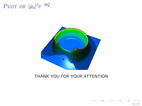
Plot of |pn|2e−NQ

THANK YOU FOR YOUR ATTENTION

32 / 32