Asymptotic Poisson Distributions with Applications to Statistical Analysis of Graphs

Asymptotic Poisson Distributions with Applications to Statistical Analysis of GraphsAuthor(s): Krzysztof NowickiSource: Advances in Applied Probability, Vol. 20, No. 2 (Jun., 1988), pp. 315-330Published by: Applied Probability TrustStable URL: http://www.jstor.org/stable/1427392 .

Accessed: 28/08/2013 04:24

Your use of the JSTOR archive indicates your acceptance of the Terms & Conditions of Use, available at .http://www.jstor.org/page/info/about/policies/terms.jsp

.JSTOR is a not-for-profit service that helps scholars, researchers, and students discover, use, and build upon a wide range ofcontent in a trusted digital archive. We use information technology and tools to increase productivity and facilitate new formsof scholarship. For more information about JSTOR, please contact [email protected].

.

Applied Probability Trust is collaborating with JSTOR to digitize, preserve and extend access to Advances inApplied Probability.

http://www.jstor.org

This content downloaded from 138.251.14.34 on Wed, 28 Aug 2013 04:24:42 AMAll use subject to JSTOR Terms and Conditions

http://www.jstor.org/action/showPublisher?publisherCode=apt

http://www.jstor.org/stable/1427392?origin=JSTOR-pdf

http://www.jstor.org/page/info/about/policies/terms.jsp


Adv. Appl. Prob. 20, 315-330 (1988) Printed in N. Ireland

? Applied Probability Trust 1988

ASYMPTOTIC POISSON DISTRIBUTIONS WITH APPLICATIONS TO STATISTICAL ANALYSIS OF GRAPHS

KRZYSZTOF NOWICKI,* University of Lund

Abstract Various types of graph statistics for graphs and digraphs are presented as

numerators of incomplete U-statistics, with symmetric and asymmetric kernels, respectively. Thus, asymptotic Poisson limits of these statistics are provided by using limit theorems for the sums of dissociated random variables. Several applications to statistical analysis of graphs are given. RANDOM GRAPHS AND DIGRAPHS; SUBGRAPH COUNTS; INCOMPLETE U-STATISTICS;

DISSOCIATED RANDOM VARIABLES; POISSON LIMIT THEOREMS

1. Introduction

The first extensive studies of random graphs were done by Erdis and R6nyi (1959), (1960). They considered undirected graphs and investigated threshold functions for subgraphs of given types, as well as the asymptotic distributions of various subgraph counts. In particular, they proved that under certain conditions the number of isolated trees and k-cycles have a Poisson limit distribution.

Recently, several authors have considered subgraph count statistics for Bernoulli graphs, i.e. undirected random graphs obtained from a complete graph on n vertices by independently deleting its edges with a common probability 1 - p. Bollobais (1981) and Karofiski and Rucifiski (1983) proved that counts of strictly balanced subgraphs tend to either a Poisson limit or a normal limit depending on how fast p tends to 0 with increasing n; see the survey article by Karotiski (1984). Nowicki (1985) represented subgraph count statistics as numerators of incomplete U-statistics and proved their normal limit for the case of a constant p.

Various kinds of statistical analyses of graph data can be based on subgraph counts. In some cases, subgraph counts are sufficient statistics, as, for example, in the case of undirected and directed Markov graphs, see Frank and Strauss (1986). However, for other models and for empirical graph data, subgraph counts are used to describe structural properties, e.g. inconsistency in pairwise comparisons, Kendall

Received 26 February 1986; revision received 19 May 1987. * Postal address: Department of Mathematical Statistics, University of Lund, Box 118, S-221 00 Lund,

Sweden. Partial support for this paper was given by the Swedish Council for Research in the Humanities and

Social Sciences under contract No. F46/84.

315



316 KRZYSZTOF NOWICKI

and Babington Smith (1940), or transitivity of contacts and friendship choices, Frank and Harary (1982).

These and other applications lead to the counting of certain subgraph types. In the case of an undirected graph, of particular interest are k-cycles, k-stars and complete graphs. For a directed graph (digraph), on the other hand, we often want to count induced subgraphs of order 2 and 3, so-called dyads and triads. Dyads can be of three non-isomorphic types depending on whether they have no edge, a single directed edge or two directed edges, respectively; while there are 16 different (non-isomorphic) triads, see Figure 2.

Most digraph models are based on the assumption of stochastic independence between dyads. This assumption leads to log-linear models with parameters representing attraction, reciprocity and other sociometric properties of networks, see Holland and Leinhardt (1981) and Fienberg et al. (1985). In that which follows we always assume that digraphs have independent dyads.

The limit distributions of subgraph counts for Bernoulli graphs and for digraphs can be useful for testing whether empirical graph data have been generated from some more complicated models than pure chance models. Such methods have been proposed by Frank (1980) for Bernoulli graphs and by Moon (1968) for investigation of random tournaments.

In this paper we study limit distributions of subgraph counts for Bernoulli graphs and for digraphs. We show how the U-statistic representation of subgraph counts can be used to prove their Poisson limit distribution by applying the results of Barbour and Eagleson (1984).

In Section 2 we will give basic concepts and notations. Section 3 gives the necessary conditions for the Poisson limit distribution of symmetric and asymmetric U-statistics. In Sections 4 and 5 we use those conditions to investigate the limit distributions of subgraph counts for Bernoulli graphs and for digraphs, respectively. Finally, in Section 6 we present various applications of subgraph counts for the statistical analysis of graphs.

2. Basic concepts and notations of random graphs

Let N be a set of n elements called vertices. Let N(2) be the set of all n(n - 1) ordered sequences of two distinct elements from N.

A graph G on N is a set of unordered pairs of vertices called edges and s = IGI is

called the size of G. The size of G can be at most(2

; such a graph is called a

complete graph and is denoted by K,,. A digraph G on N is a subset of N(2) with elements in G called directed edges.

Moreover, if a pair (u, v) belongs to G we say that there is a directed edge from u to v.



Asymptotic Poisson distributions 317

If A is a subset of N, any graph or digraph on A contained in G is called a subgraph of G and v = IAI is called the order of the subgraph. In this paper we study subgraphs of random graphs defined by specifying their set of edges, i.e. subgraphs without isolated vertices.

A subgraph H of G is called an induced subgraph if there is a subset B of N such that all subgraphs on B are contained in H.

Two graphs or digraphs G and H are isomorphic if there exists a bijection between their vertex sets which maps G into H.

Suppose that G is a graph of size s and order v and define the degree of G as d = s/v. A graph G is strictly balanced if it contains only subgraphs whose degrees are smaller than the degree of graph G. Moreover, a necessary but not sufficient condition for graph G to be strictly balanced is that G does not have isolated vertices.

3. Poisson limit distributions for T-statistics

Let X1, - --, X, be independent, identically distributed random variables and

g(xl, .... , Xk) a zero-one function, symmetric or asymmetric, which we call a kernel. Introduce the statistic

(3.1) To=$gi i=1

where the gi's are obtained by inserting the (n) possible ordered subsequences

Xr, . ..Xr, r, 1 < r1 < ' . <rk 5 n in g, the numbering of the gi's being arbitrary.

We may call To a complete T-statistic. By suitable choice of the function g the statistic To can be used to count the number of certain configurations in data. In the analysis of random graphs, for example, we set X, = 1 if an edge i is present in the observed graph and let g(X,, - - -

Xk)= 1 if edges il, * * *, ik are present. Then To counts the number of all subgraphs with k edges; see Nowicki (1985).

Silverman and Brown (1978) investigated the limit distribution of To under the assumption that the kernel is symmetric and proved that

To > Poisson (A)

as n--- oo under the following conditions on the distribution of the random variables Xr:

and 2k-1~ik-1 0




where p = Eg(X1, ..., Xk)

and

_k-1 = E(g(X1, . . . , Xk)g(X2, . . .

, Xk+1)).

Introduce now

m

(3.2) T = g i=1

where the gi's are obtained by inserting m of the (k) possible ordered k

subsequences of X1, ... , X, in g. We call this an incomplete T-statistic. Nowicki (1985), (1986) represented various types of subgraph count statistics as well as triad counts as incomplete T-statistics with a symmetric or an asymmetric kernel and proved the asymptotic normality of these statistics for Bernoulli graphs and random digraphs.

Even incomplete T-statistics sometimes have a Poisson distribution in the limit. Barbour and Eagleson (1984) generalized the result of Silverman and Brown (1978) by formulating general conditions for the Poisson limit distribution of dissociated statistics. We will use their results to give conditions for the Poisson limit distribution of T-statistics, both for symmetric and asymmetric kernels.

Consider an incomplete T-statistic (3.2). The random variables gl, " ", gm form

m2 pairs (gi, gj) = 1. Let fc, c = 1, , k be the number of pairs with c X-values in common. For a symmetric function g we set

Ic = E(g(X1, ... , Xk)g(X1, .. , Xc, Xk+l, ..., X2k-c)) i.e. Mc is the expectation of the product of two g's with c arguments in common. Then, for a symmetric kernel we obtain the following result.

Theorem 1. If, for n -oo

(3.3) mpA-- and m---oo

and k-1

(3.4) fclc O 0 c=1

then

T -D Poisson (A).

Proof. The theorem can be deduced from Theorem 2 of Barbour and Eagleson




(1984). Their conditions, modified for T-statistics defined as in (3.2), are as follows:

(3.5) mp -> A

(3.6) mp2 + > (p2 + Eg~gi)-->

0

where the sum is taken over pairs gi, gj with at least one and at most k - 1 X-values in common.

First, since the kernel is symmetric, Egigj depends only on the number of common X-values in gi and gj. Since there are fl, "

, fk-1 pairs with 1, .

, k - 1 X-values in common, respectively, we obtain

k-1

S(p2 +Eggj)= fc(p2 + ). c=1

Second, as proved by Hoeffding (1948) we have that

Pc = Eh(Xl,"',

Xc), c = 1,.,

k- 1

where

hc(xl, " "

, Xc) = E(g(X1, , Xk) I X1 = X1, "

, Xc =Xc).

Thus we can write

V(hc(X1, . , Xc))

= PC -P2

which gives

0• p2 + 2_c.

Consequently, condition (3.6) holds if k-1

(3.7) mp2 + 2 Z fcc -> O.

c=1

Finally, since condition (3.3) gives that mp2- 0 we obtain that (3.7) follows from (3.4).

When g is asymmetric, Theorem 2 of Barbour and Eagleson (1984) leads to the following result.

Theorem 2. If, for n -> oo

(3.8) mp -> A

and

k

(3.9) p2 c

fc +

, E(g

g)---O 0

c=1




where the last sum is taken over all pairs of subsequences with at least one X-value and at most k - 1 X-values in common, then

T -D Poisson (A).

4. Poisson limit of subgraph count statistics for Bernoulli graphs

Consider a Bernoulli graph G on a finite set {1, - - - , n} of vertices, i.e. a graph whose edges occur independently with the same probability p, 0<p <1. The

probability of an edge is a function of the number of vertices. Such a graph can be

described by a set of (n) independent random variables, Xt,, 1 5 t < u n, where

{ 1 if an edge occurs between vertices t and u = 0 otherwise.

We want to count the number of subgraphs of G with prescribed properties. For example, we may count the number of subgraphs of G isomorphic to a given subgraph H of size s and order v.

For this purpose, let us introduce the symmetric kernel

g(xl, s x,) = X1X2' ' 's

and the incomplete T-statistic

m (4.1) T = gi.

i=1

Here the gi's are obtained by inserting m suitably chosen subsequences taken from the set

{Xt•} in g. Clearly, g = 1 if and only if all X,, corresponding to the ith

subsequence are equal to 1. For example, take s = 3, n = 4 and let H be a triangle, i.e. a complete graph on

three vertices. The T-statistic

T = g(X12, X13, X23) + g(X12, X14, X24) + g(X13, X14, X34) + g(X23, X24, X34)

counts the number of triangles in G. Nowicki (1985) used (4.1) for investigating the asymptotic normality of subgraph

count statistics for Bernoulli graphs with constant p. Modifying the summation, (4.1) can also be used for counting the number of all

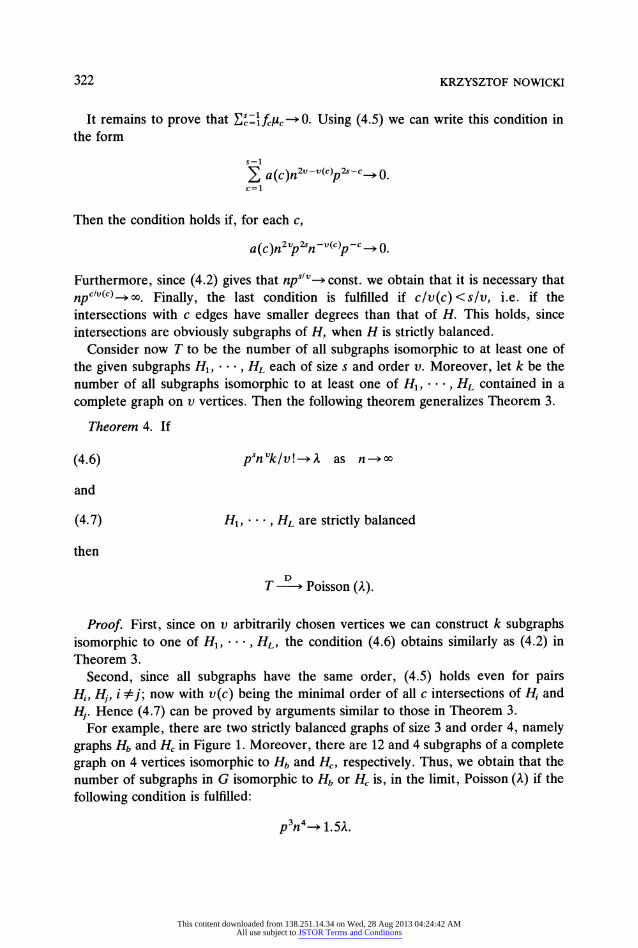
subgraphs isomorphic to at least one of the given graphs H1, -'", HL, each of size s. For example, we want to count the number of connected subgraphs with three edges, i.e. the subgraphs isomorphic to one of the graphs in Figure 1.

We will now prove that subgraph count statistics tend to a Poisson limit under certain conditions. Bollobis (1981) and Karoiiski and Rucifiski (1983) considered a




Hd Fi

Figure 1.

family TP of strictly balanced graphs each of size s and order v. They gave conditions on p required for obtaining a Poisson limit distribution for the number of subgraphs in G isomorphic to at least one graph in P. (See the survey article by Karoriski (1984).) We will show that their results can be obtained as a consequence of Theorem 1.

Let T be defined as in (4.1). Moreover, let s be the size of H and v its order, and k, the number of all subgraphs isomorphic to H contained in a complete graph on v vertices; H, s, v and k, are fixed as n - oo. Then we have the following result.

Theorem 3. If

(4.2) psnk ,/v!--- as n--oo

and

(4.3) H is strictly balanced

then T -D Poisson (A).

Proof. First, by the definition of the kernel g we obtain

Eg(Xl, I . . , X,) =

E(XIX2 .

. X,) =pS

and

y, = E(X2X2. - -

X2Xi+l. . . X2,-i) p2-i, i = 1, . . , S.

Second, since on v arbitrarily chosen vertices we can construct k, subgraphs isomorphic to H, condition (3.3) of Theorem 1 gives

(4.4) k,( )ps" A

which leads to (4.2). Third, we notice that counting pairs gi, gj with c X-values in common is equivalent to counting pairs H,, Hj of subgraphs in a complete graph K,, where both Hi and

H. are isomorphic to H and

H-,n Hj I = c. Thus, fc, c =

1, ... , s - 1 is equal to the number of all possible subgraphs in K,, with c edges arising as the intersection of two graphs isomorphic to H. Hence, we obtain

(4.5) fc - a(c)n2v-v(c)

where v(c) is the minimal order of all c intersections; a(c) and v(c) do not depend on n.




It remains to prove that c1cIc~

0. Using (4.5) we can write this condition in the form

s-1

> a(c)n2v-v(c)p2s-c 0. C=1

Then the condition holds if, for each c,

a(c)n2vp2'n-v(c)p-c- 0.

Furthermore, since (4.2) gives that np"--- const. we obtain that it is necessary that

npc/(c)---.oo Finally, the last condition is fulfilled if clv(c)<s/v, i.e. if the intersections with c edges have smaller degrees than that of H. This holds, since intersections are obviously subgraphs of H, when H is strictly balanced.

Consider now T to be the number of all subgraphs isomorphic to at least one of the given subgraphs H1, - - - , HL each of size s and order v. Moreover, let k be the number of all subgraphs isomorphic to at least one of H1, - - - , HL contained in a complete graph on v vertices. Then the following theorem generalizes Theorem 3.

Theorem 4. If

(4.6) pSnvk/v!--- as n---oo

and

(4.7) H1, - H , HL are strictly balanced

then

D

T -~ Poisson (A).

Proof. First, since on v arbitrarily chosen vertices we can construct k subgraphs isomorphic to one of H1, ... , IHL, the condition (4.6) obtains similarly as (4.2) in Theorem 3.

Second, since all subgraphs have the same order, (4.5) holds even for pairs H,, Hi, i $j; now with v(c) being the minimal order of all c intersections of H, and H,. Hence (4.7) can be proved by arguments similar to those in Theorem 3.

For example, there are two strictly balanced graphs of size 3 and order 4, namely graphs Hb and Hc in Figure 1. Moreover, there are 12 and 4 subgraphs of a complete graph on 4 vertices isomorphic to Hb and

Hc, respectively. Thus, we obtain that the

number of subgraphs in G isomorphic to iHb or Hc

is, in the limit, Poisson (A) if the following condition is fulfilled:

p3n4 -1.5A.




5. Poisson limit distribution of triad count statistics for digraphs

Consider a digraph G on a finite set {1, ... , n} of vertices. Such a graph can be

described by the set of (n) independent random variables Xt,,

15 t < u 5 n, where

0 if no edge between t and u 1 if an edge from t to u and no edge from u to t

-1 if an edge from u to t and no edge from t to u 2 if edges from t to u and from u to t.

Furthermore, let po, Pi and P2 denote the probabilities for outcomes 'no edge', 'single edge' and 'mutual edge', respectively. Moreover, we shall consider only the situations where two directed edges are equally probable, i.e. each of the outcomes 1 and -1 has probability p = p1/2.

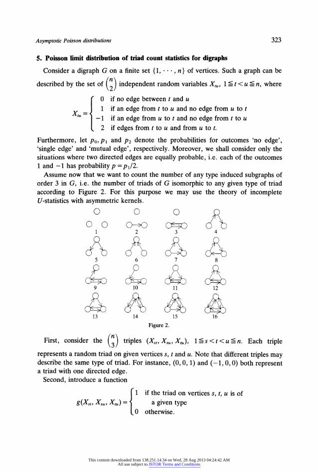
Assume now that we want to count the number of any type induced subgraphs of order 3 in G, i.e. the number of triads of G isomorphic to any given type of triad according to Figure 2. For this purpose we may use the theory of incomplete U-statistics with asymmetric kernels.

00 0-> C-O 1 2 3 4

5 6 7 8

9 10 11 12

13 14 15 16

Figure 2.

(n) First, consider the 3 triples (X,,, X,,, X,), 1 - s < t < u - n. Each triple

represents a random triad on given vertices s, t and u. Note that different triples may describe the same type of triad. For instance, (0, 0, 1) and (-1, 0, 0) both represent a triad with one directed edge.

Second, introduce a function

1 if the triad on vertices s, t, u is of g(X,,, X,,, Xu)=

j a given type 0 otherwise.




Observe that in the case of digraphs, g is not always symmetric. Consider, for example, a triad with two directed edges both pointing into the same vertex, i.e. the triad of type 6 in Figure 2. Then the following outcomes of (X X,,, X,,) describe a triad isomorphic to this triad: (-1, -1, 0), (0, 1, 1) and (1, 0, -1). Hence in this case we define g by

g(x, y, z) = I(x = - 1)I(y = -1)I(z = 0) + I(x = O)I(y = 1)I(z = 1) (5.1) + I(x = 1)I(y = O)I(z = -1)

where I(x = 1) indicates whether or not x = 1. Thus an incomplete T-statistic

T= 9gi i=1

where the gi's are obtained by inserting in g all subsequences Xs, Xu, Xtu, 1 - s < t < u 5 n counts the triads of a given type. We now give conditions under which triad count statistics tend to a Poisson limit

distribution. Let T denote the number of triads of type i with respective kernel g', set Pi = Eg' and h'(X1) = E(g'(X1, X2, X3) I X1). Then we obtain from Theorem 2 the following result.

Theorem 5. If

(5.2) (3nP'->A as n->oo

and

(5.3) n4E(hi)2-> 0 as n ->

then

D

-~-D Poisson (A).

Proof. Condition (5.2) is the same as condition (3.8) of Theorem 2. To prove that condition (3.9) holds observe first that in a pair gi, gj the g's have either no X's in common, one X in common or all three X's in common (in what follows we use g to denote any kernel, gl, ... , g16). Hence, the last sum in (3.9) contains only pairs

with one X in common. Moreover, there are 2() (n22)- and-(n) pairs with one 2 2 3

and three X's in common, respectively. Since condition (5.2) implies that n6P2-• const. we obtain that

3

P: fc-> O. c=l




Second, we calculate the expectations E(gigj) in (3.9). Conditional on the common argument X the functions gi and gj are independent. Hence

E(gigj) = E(E(gi I X)E(gj I X)). Now we prove that the conditional expectation of kernel g is not affected if we

condition it on the first, second or third argument. By definition each kernel is a sum of terms of the form I(X,, = x,,)I(X,, = x,,)I(Xtu = x,t), x,,, x,,, x,, = 0, 1, -1 or 2. The set of outcomes (x,,, x,, ) used to construct a kernel is obtained in the following way: we consider all six labeled triads on vertices s, t, u which are isomorphic to a given type of triad; this gives us a set of, at most, six different outcomes (xs,, xsu, x,). Next, we turn to calculating h1, h2 and h3, which are the conditional expectations of the kernel given Xst, Xs, and Xu, respectively. Observe that to obtain, for example, h1(1) we use only terms containing the expression I(Xs= 1). The conditional expectation of each such term is equal to I(X,, =

1)p2-A-BpApB where A and B are the total number of single and mutual edges respectively between vertices s and u and between vertices t and u. Moreover, the same number of terms in the kernel contain I(Xsu = 1) and I(Xtu = 1), respectively. Hence hi, h2, h3 are identically distributed random variables, which we call h. Finally, the number of terms in the sum has the order of magnitude n4 which gives (5.3).

Let us now use Theorem 5 to find conditions on Po, p and p2 required for obtaining a Poisson limit distribution for T6. By using (5.1) we calculate

and Eg6 = 3p2p0

E(g6 I X) =pop(I(X = 1) + I(X = -1)) +p21(X = 0).

Thus, the conditions (5.2) and (5.3) of Theorem 5 can now be stated in the following form:

(5.4) 33p2_> A

and

(5.5) n4(2pop3 p4p)--0

and by inserting (5.4) into (5.5) we obtain

3(n)p20__>A np2--_0.

6. Applications

Random graphs, both undirected and directed, have been used in many areas as models of data for binary relationships between the elements in a set. This set might, for instance, consist of people (sociology, social psychology), the components




of a system (reliability theory), particles (physics) or different divisions of a company (operations research).

Undirected graphs represent symmetric relationships, i.e. ones in which every two elements can either be related or unrelated to each other. For instance, in cluster analysis it is desirable to partition a set of objects into subsets of similar objects (clusters) by using information about pairwise similarities or dissimilarities between the objects.

Directed graphs, on the other hand, are used for data associated with an

asymmetric relation. In paired comparisons experiments, for instance, a directed graph can indicate which element within each pair is 'better'. Such a paired comparisons procedure, called a complete tournament, can be used to order elements. Other types of tournaments are tournaments with ties and knock-out tournaments. In the former, some comparisons may not distinguish the 'better' player. In the latter, the winners from each game play each other in series of rounds to obtain one final winner.

In the analysis of social networks we may study the friendship relationships within a school class obtained by asking the children to name their best friends in the class. Then friendship can be represented by a directed graph and mutual friendship by an undirected graph. For more references on social networks see, for example, Holland and Leinhardt (1979) or Knoke and Kuklinski (1982).

Several questions of interest about pattern detection and measurement of structures in social networks can be formulated in terms of subgraph counts. For instance, subgraph counts can be used to investigate transitivity and consistency. A symmetric relation is transitive if (u, w) is a related pair of elements whenever (u, v) and (v, w) are related pairs. There are many aspects of pairwise relations, for instance clustering or partial orderings, which are affected by transitivity. A transitive relation leads to a graph which consists of one or more complete components.

Several authors have proposed and investigated indices for measuring transitivity e.g. Harary and Kommel (1979), Holland and Leinhardt (1971, 1979), Frank (1980) and Frank and Harary (1982). A simple transitivity index is

(6.1) r= /(t3

i.e. the proportion of triangles (graphs of order 3 and size 3) in a graph. In order to be able to judge whether an empirical graph has a significantly high or

low degree of transitivity, we need to know the distribution of the transitivity index under a null hypothesis which specifies a pure chance model. Such a model can be

specified by assuming a Bernoulli graph in which p = r 2 where r is the number

of edges in the empirical graph. In this way we obtain a stochastic graph with the same expected number of edges as in the empirical graph.




Different properties of social networks lead to various types of asymptotic distributions of r under such a null hypothesis. Nowicki (1985) considered a case in which the probability p of a relation between two individuals does not depend on the size n of the group. Thus, he obtained that r is normally distributed.

Here, on the other hand, p is a function of n for which we assume that

p = O(1/n). For instance, we may think of a network with a fixed expected number of edges adjacent to each vertex. Thus using the result of Theorem 3 we can establish the asymptotic distribution for r.

Theorem 6. Let r be a transitivity index defined as in (6.1). Then under a pure chance model, i.e. for a Bernoulli graph with parameters n and p = O(1/n), we obtain

P(() = k)- A•

exp(-A)/k!

where

Now we turn to the question of consistency. Ranking the objects using pairwise comparisons often, particularly in psychological work, raises the question of whether the data itself is suitable for ranking. Preferences can be established according to a number of factors and we may thus doubt if a final preference can be expressed on a linear scale. Assume, for instance, that for three given objects u, v and w, we observed the following preferences u -- v -- w -- u or u <- v <-- w <-- u, (u -- v means that v is preferred to u), i.e. there is a 3-cycle on u, v and w. Thus, objects u, v and w can not be ranked. Kendall and Babington Smith (1940) proposed an index based on the number of 3-cycles as a measure of consistency in a tournament.

In order to test the departure of given data from consistency Moran (1947) considered a tournament where its directed edges are independent with equal probability for both directions and proved that then this index is normally distributed; also see Moon (1968). An extension of this index by including ties, i.e. situations when two objects are indistinguishable or no preferences between two objects can be stated, has been studied by Nowicki (1986). Even such an index is asymptotically normally distributed.

However, it is impractical to carry out all comparisons and only then to discover that the pairwise comparisons are in fact inconsistent. Comparisons are often both time-consuming and expensive and since every object must be compared to all other objects, even a medium-sized group requires a considerable number of comparisons. Thus, the following method can be used to reduce the number of pairwise comparisons necessary to investigate the consistency of the procedure.

Consider a group which consists of n objects so that there is a set of (") pairs of these objects. However, we reduce this set by randomly deleting its elements with




the probability 1 - P, independently for each pair. Thus, we obtain an incomplete tournament, i.e. one in which we have the probability P that a given pair of objects participates in it.

Theorem 7. Let c3 denote the number of 3-cycles in an incomplete random tournament with the probability P that a given pair of objects participates in it; P = O(1/n). Moreover, given that the pair (u, v) participates in the tournament, we assume equal probability for both directions. Then

P(c3 = k) A-

k exp (-A)/k! where

A = ()P3/4.

Proof. The result follows from Theorem 5, where we set Po = 1 - P, p = P/2 and P2 =

0.

In order to study the reliability of systems or networks, as for instance their failure or non-failure over a period of time, we represent them in the form of connected components. The state of a system where connections and(or) components either fail or are operative can be described by binary variables. This can apply to, for example, electrical systems, networks of computers or communication networks. (For references see, for instance Barlow and Proschan (1965), (1975)). Moore and Shannon (1956) introduced a reliability model for binary networks by letting components and connections fail randomly, all failures being independent and having known probabilities. This can be conveniently represented by a random graph, where connections and components are represented by edges and vertices, respectively.

Several aspects of reliability have been expressed in terms of properties of graphs. Gilbert (1959) studied the network of telephone offices for which connections between centrals fail independently with a common probability. He obtained the probability that any two offices can reach each other, either directly or via other offices, i.e. the probability that the corresponding Bernoulli graph is connected. Frank and Gaul (1982) extended this result to graphs with randomly failing vertices and edges. However, the disconnection of the graph does not measure the partial usefulness of the system, since for networks of substantial size there will frequently be one or more vertices which is disconnected from the rest. An alternative measure of the reliability of networks is given by the probability that two specified vertices are connected.

The above-mentioned measures of a network's reliability are based on connec- tivity. However, the usefulness of a network can be related to other structural properties. A network can be functioning provided that it has at least k components of a certain property. Thus, reliability measures based on subgraph counts can be of interest.




Other interesting problems are associated with the design of systems in which certain reliability requirements must be met. For instance, consider a system of n reliable components with connections failing randomly, with the same probability p; n >> 1. We want to guarantee that, with the given probability Po, at least a certain number of triples remains connected, i.e. that P(t ? to) ? Po where t is the number of triangles. Thus, using the asymptotic distribution of t we can obtain the minimal expected number of triangles, such that this condition is fulfilled and consequently the required higher bound for p.

Acknowledgement

I am indebted to Professor Gunnar Blom and Professor Ove Frank for kindly offering their time for discussion, valuable suggestions and comments. I also want to thank the referee whose valuable comments led to significant improvements in this paper.

References

BARBOUR, A. D. AND EAGLESON, G. K. (1984) Poisson convergence for dissociated statistics. J. R. Statist. Soc. B 46, 397-402.

BARLOW, R. E. AND PROSCHAN, F. (1965) Mathematical Theory of Reliability. Wiley, New York. BARLOW, R. E. and PROSCHAN, F. (1975) Statistical Theory of Reliability and Life Testing. Holt, New

York. BOLLOBAS, B. (1981) Threshold functions for small subgraphs. Math. Proc. Camb. Phil. Soc. 90,

197-206. ERD6s, P. AND RENYI, A. (1959) On random graphs 1. Publ. Math. Debrecen 6, 290-297. ERD6s, P. AND RENYI, A. (1960) On the evolution of random graphs. Publ. Math. Inst. Hung. Acad.

Sci. 5, 17-61. FIENBERG, S., MEYER, M. AND WASSERMAN, S. (1985) Statistical analysis of multiple sociometric

relations. J. Amer. Statist. Assoc. 80, 51-67. FRANK, 0. (1980) Transitivity in stochastic graphs and digraphs. J. Math. Sociol. 7, 199-213. FRANK, O. AND GAUL, W. (1982) On reliability in stochastic graphs. Networks 12, 119-126. FRANK, O. AND HARARY, F. (1982) Cluster inference by using transitivity indices in empirical graphs.

J. Amer. Statist. Assoc. 77, 835-840. FRANK, O. AND STRAUSS, D. (1986) Markov graphs. J. Amer. Statist. Assoc. 81, 832-842. GILBERT, E. N. (1959) Random graphs. Ann. Math. Statist. 30, 1141-1144. HARARY, F. AND KOMMEL, H. (1979) Matrix measures for transitivity and balance. J. Math. Sociol. 6,

199-210. HOEFFDING, W. (1948) A class of statistics with asymptotically normal distribution. Ann. Math.

Statist. 19, 293-325. HOLLAND, P. AND LEINHARDT, S. (1971) Transitivity in structural models of small groups.

Comparative Group Studies 2, 107-124. HOLLAND, P. AND LEINHARDT, S. (EDS) (1979) Perspectives on Social Network Research. Academic

Press, New York. HOLLAND, P. AND LEINHARDT, S. (1981) An exponential family of probability distributions for

directed graphs. J. Amer. Statist. Assoc. 76, 33-51. KARON1SKI, M. (1984) Balanced Subgraphs of Large Random Graphs. Uniwersytet im. Adama

Mickiewicza w Poznaniu, Seria Matematyka nr. 7. KARONSKI, M. AND RUCIlSKI, A. (1983) On the number of strictly balanced subgraphs of a random

graph. Graph Theory, Lag6w 1981. Lectures Notes in Mathematics 1018, Springer-Verlag, 79-83.




KENDALL, M. AND BABINGTON SMITH, B. (1940) On the method of paired comparisons. Biometrika 31, 324-345.

KNOKE, D. AND KUKLINSKI, J. H. (1982) Network Analysis. Sage Publications, Beverly Hills. MOON, J. W. (1968) Topics in Tournaments. Holt, New York. MOORE, E. F. AND SHANNON, C. E. (1956) Reliable circuits using reliable relays. J. Franklin Inst. 262,

191-208; 281-297. MORAN, P. A. (1947) On the method of paired comparisons. Biometrika 34, 363-365. NOWICKI, K. (1985) Asymptotic normality of graph statistics. J. Statist. Planning Inf. To appear. NOWICKI, K. (1986) Asymptotic normality of triad counts for directed graphs. University of Lund,

Stat. Res. Rep. 1986:7, 1-17. SILVERMAN, B. AND BROWN, T. (1978) Short distances, flat triangles and Poisson limit. J. Appl. Prob.

15, 815-825.



Documents

Asymptotic Poisson Distributions with Applications to Statistical Analysis of Graphs