Asymptotic Nearest Rules Using Data - UGRsci2s.ugr.es/keel/pdf/algorithm/articulo/1972-Wilson-IEEETSMC.pdf · rules and the nearest neighbor rules using edited preclassified samples

IEEE TRANSACTIONS ON SYSTEMS, MAN, AND CYBERNETICS, VOL. SMC-2, NO. 3, JULY 1972

Asymptotic Properties of Nearest NeighborRules Using Edited Data

DENNIS L. WILSON, MEMBER, IEEE

Abstract-The convergence properties of a nearest neighbor rule thatuses an editing procedure to reduce the number of preclassified samplesand to improve the performance of the rule are developed. Editing of thepreclassified samples using the three-nearest neighbor rule followed byclassification using the single-nearest neighbor rule with the remainingpreclassified samples appears to produce a decision procedure whose riskapproaches the Bayes' risk quite closely in many problems with only a

few preclassified samples. The asymptotic risk of the nearest neighborrules and the nearest neighbor rules using edited preclassified samples iscalculated for several problems.

1. INTRODUCTION

A BASIC class of decision problems which includes a

large number of practical problems can be charac-terized in the following way. I) There is a sample to beclassified. 2) There are already classified samples from thesame distributions as the sample to be classified with whicha comparison can be made in making a decision. 3) Thereis no additional information about the distributions of any

of the random variables involved other than the informationcontained in the preclassified samples. 4) There is a measure

of distance between samples. Examples of problems havingthese characteristics are the problems of handwritten charac-ter recognition and automatic decoding of manual Morse.In each of these problems preclassified samples may beprovided by a man, and a simple metric can be devised.

"Nearest neighbor rules" are a collection of simple ruleswhich can have very good performance with only a fewpreclassified samples. We shall develop the asymptotic per-

formance of a nearest neighbor rule using editing. Theasymptotic performance is the performance when thenumber of preclassified samples is very large.

Nearest neighbor rules were originally suggested forsolution of problems of this type by Fix and Hodges [I] in

1952. Nearest neighbor rules are practically always in-

cluded in papers which survey pattern recognition, e.g.,

Sebestyen [2], Nilsson [3], Rosen [4], Nagy [5], and Hoand Agrawala [6]. Analysis of the properties of the nearestneighbor rules was started by Fix and Hodges [I] andcontinued by Cover and Hart [7] and Whitney and Dwyer[8]. Cover [9] summarizes many of the properties of thenearest neighbor rules. Patrick and Fischer [10] generalizethe nearest neighbor rules to include weighting of differenttypes of error and problems "in which the training samplesavailable are not in the same proportions as the a prioriclass probabilities" by using the concept of tolerance regions.

Manuscript received September 16, 1970; revised December28, 1971.The author is with the Electronic Systems Group-Western Division,

GTE Sylvania, Inc., Mountain View, Calif. 94040.

The nearest neighbor decision procedures use the sampleto be classified and the set of preclassified samples in makinga decision.

The Sample to Be ClassifiedLet Xe Ed be a random variable generated as follows.

Select 0 = I with probability t1 and 0 = 2 with prob-ability t12. Given 0, select X from a population with densityfi(x) when 0 = I and from a population with densityf2(x)when 0 = 2 (Ed is a d-dimensional Euclidean space).

The Preclassified SamplesLet (Xi,Oi), i = 1,2, ,N, be generated independently

as follows. Select Oi = I with probability ?1I and 0, = 2with probability 72. Given 0,, select Xi EEd from a popula-tion with densityf1(x) when Oi = I and from a populationf2(x) when Oi = 2. The set {(Xi,O,)} constitutes the set ofpreclassified samples.Two types of rules will be discussed: nearest neighbor

rules and modified nearest neighbor rules.To make a decision using the K-nearest neighbor rule:

Select from among the preclassified samples of the K-nearestneighbors of the sample to be classified. Select the classrepresented by the largest number of the K-nearest neigh-bors. Ties are to be broken randomly.To make a decision using the modified K-nearest neighbor

rule:

a) For each i,I) find the K-nearest neighbors to X, among

(XI,X2, - ,Xi- ,,X,+ X, ,XN};2) find the class 0 associated with the largest number

of points among the K-nearest neighbors, break-ing ties randomly when they occur.

b) Edit the set {(X,,O,)} by deleting (Xi,O,) whenever 0,does not agree with the largest number of theK-nearest neighbors as determined in the foregoing.

Make a decision concerning a new sample using the modifiedK-nearest neighbor rule by using the single-nearest neighborrule with the reduced set of preclassified samples.

Examples of the Power of the Nearest Neighbor RulesThe nearest neighbor rules can be very powerful rules,

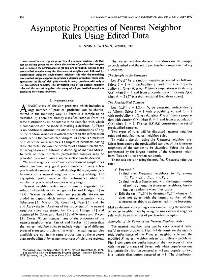
useful in many problems. Figs. 1-4 demonstrate the asymp-totic performance of the K-nearest neighbor rule and themodified K-nearest neighbor rule in four different problems.Fig. I compares the performance of the two types of ruleswith the performance of Bayes' rule when population oneis a logistic distribution centered at - I and population twois a logistic distribution centered at + 1. The distribution

408

Authorized licensed use limited to: UNIVERSIDAD DE GRANADA. Downloaded on May 22, 2009 at 07:38 from IEEE Xplore. Restrictions apply.

WILSON: PROPERTIES OF NEAREST NEIGHBOR RULES

.-X K-NEAREST NEIGHBORRULE

._^ MODIFIED K-NEARESTNEIGHBOR RULE

1 0.4

0.3

co

y- 0.2.

le

L^

0.5

.-I

,___ $^_.-t.- -_:Z=z ts=

>?BAYES'OR M IN IMUMPOSSIBLE RISK

0.4

0.3

0.2

0.10.1I

012 3 4 5 io K 20Fig. 1. Asymptotic risk of using K-nearest neighor rule and the

modified K-nearest neighbor rule compared to Bayes' risk whennl = q2 = 0.5 and population one is logistic centered at - 1 andpopulation two is logistic centered at + 1.

---: -,- .- - =- ---

> BAYES'OR MINIMUMPOSSIBLE RISK

O 1 2 3 4 5 10 K 20

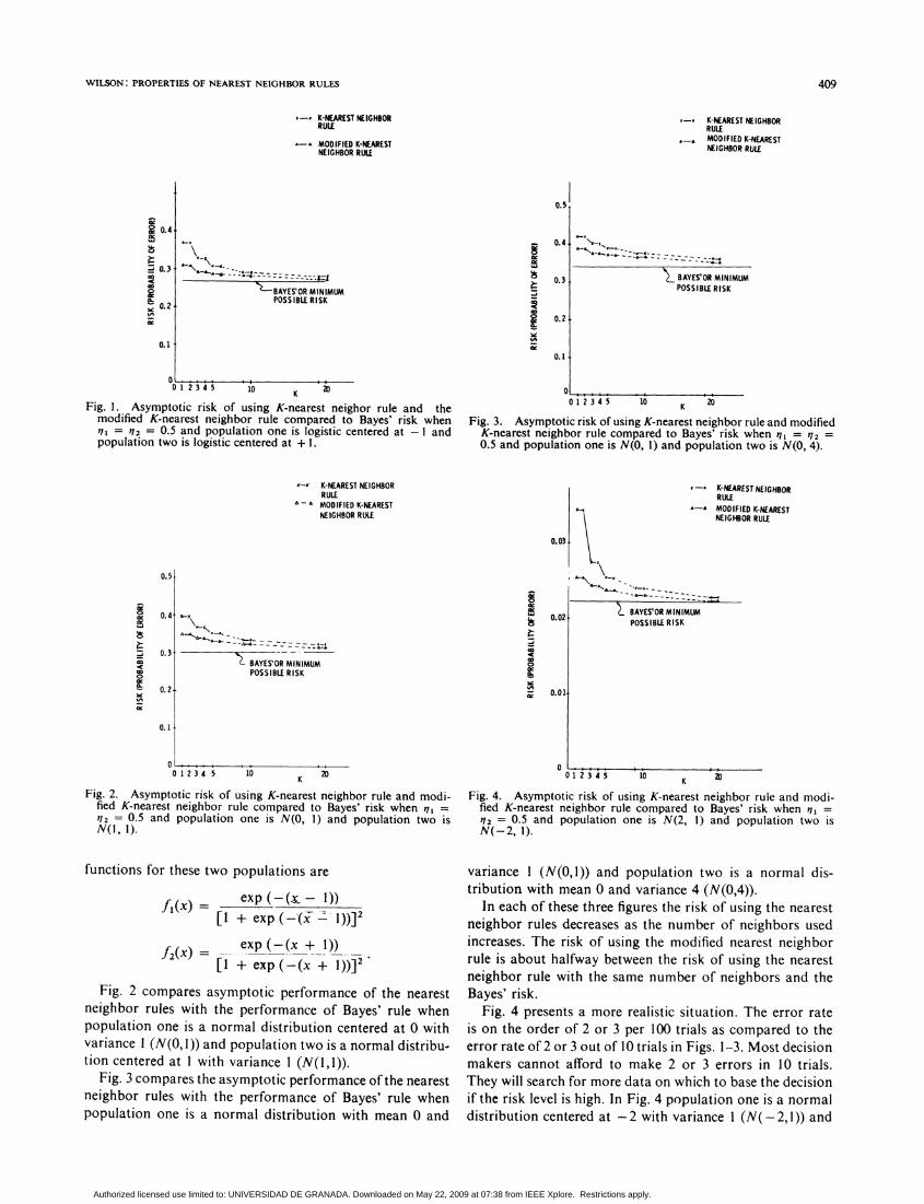
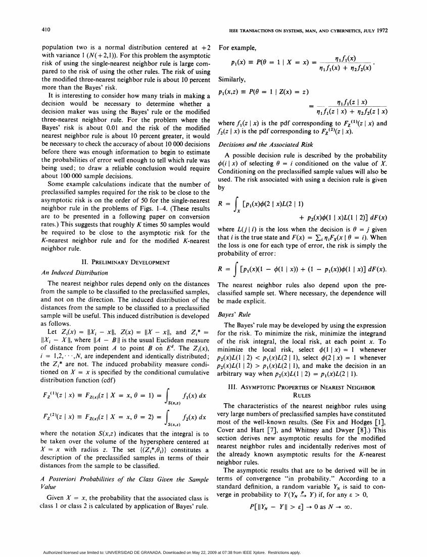
Fig. 3. Asymptotic risk of using K-nearest neighbor rule and modifiedK-nearest neighbor rule compared to Bayes' risk when 711 = 112 =0.5 and population one is N(O, 1) and population two is N(O, 4).

x-x K-NEAREST NEIGHBORRULE

" - " MODIFIED K-NEARESTNEIGHBOR RULE

0.5

0.4

1.3

-k_&k&__

-,J _' ===_7 ==_7Z-7 _

L BAYES'OR MINIMUMPOSSIBLE RISK

0.21J

x-x K-NEAREST NEIGHBORRU E

'-' MODIFIED K-NEARESTNEIGHBOR RULE

0.03

0.02 & BAYES'OR MINIMUMPOSSIBLE RISK

g

4:

-jcC'

0.01.

0.1

O x.,.. ,0 1 2 3 4 5 10 K 20

Fig. 2. Asymptotic risk of using K-nearest neighbor rule and modi-fied K-nearest neighbor rule compared to Bayes' risk when 71 =?I2 = 0.5 and population one is N(O, I) and population two isN(l, 1).

I1 2 3 4 5 10K D

0

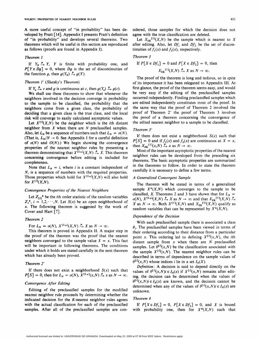
Fig. 4. Asymptotic risk of using K-nearest neighbor rule and modi-fied K-nearest neighbor rule compared to Bayes' risk when ,1 ='12 = 0.5 and population one is N(2, 1) and population two isN(-2, 1).

functions for these two populations are

(x) exp (-(x- 1))

[1 + exp (-1(x_- ))]2

f(x)- exp (-(x + 1))f2 _X= ..

[1 + exp(-(x + 1))]2

Fig. 2 compares asymptotic performance of the nearestneighbor rules with the performance of Bayes' rule whenpopulation one is a normal distribution centered at 0 withvariance I (N(O, 1)) and population two is a normal distribu-tion centered at 1 with variance 1 (N(l,l)).

Fig. 3 compares the asymptotic performance of the nearestneighbor rules with the performance of Bayes' rule whenpopulation one is a normal distribution with mean 0 and

variance 1 (N(O,I)) and population two is a normal dis-tribution with mean 0 and variance 4 (N(0,4)).

In each of these three figures the risk of using the nearestneighbor rules decreases as the number of neighbors usedincreases. The risk of using the modified nearest neighborrule is about halfway between the risk of using the nearestneighbor rule with the same number of neighbors and theBayes' risk.

Fig. 4 presents a more realistic situation. The error rateis on the order of 2 or 3 per 100 trials as compared to theerror rate of 2 or 3 out of 10 trials in Figs. 1-3. Most decisionmakers cannot afford to make 2 or 3 errors in 10 trials.They will search for more data on which to base the decisionif the risk level is high. In Fig. 4 population one is a normaldistribution centered at -2 with variance I (N(-2,1)) and

- NEAREST NEIGHBORRULE

a-, MODIFIED K-NEARESTNEIGHBOR RLXE

0

m

co-Cco0at

U .

.. ,f .

.,,,, . .

409

if9exCAC1.1

.5-j

ViIC4A

cg

0


IEEE TRANSACTIONS ON SYSTEMS, MAN, AND CYBERNETICS, JULY 1972

population two is a normal distribution centered at + 2with variance 1 (N(+ 2,1)). For this problem the asymptoticrisk of using the single-nearest neighbor rule is large com-pared to the risk of using the other rules. The risk of usingthe modified three-nearest neighbor rule is about 10 percentmore than the Bayes' risk.

It is interesting to consider how many trials in making adecision would be necessary to determine whether adecision maker was using the Bayes' rule or the modifiedthree-nearest neighbor rule. For the problem where theBayes' risk is about 0.01 and the risk of the modifiednearest neighbor rule is about 10 percent greater, it wouldbe necessary to check the accuracy of about 10 000 decisionsbefore there was enough information to begin to estimatethe probabilities of error well enough to tell which rule wasbeing used; to draw a reliable conclusion would requireabout 100 000 sample decisions.Some example calculations indicate that the number of

preclassified samples required for the risk to be close to theasymptotic risk is on the order of 50 for the single-nearestneighbor rule in the problems of Figs. 1-4. (These resultsare to be presented in a following paper on conversionrates.) This suggests that roughly K times 50 samples wouldbe required to be close to the asymptotic risk for theK-nearest neighbor rule and for the modified K-nearestneighbor rule.

II. PRELIMINARY DEVELOPMENTAn Induced DistributionThe nearest neighbor rules depend only on the distances

from the sample to be classified to the preclassified samples,and not on the direction. The induced distribution of thedistances from the sample to be classified to a preclassifiedsample will be useful. This induced distribution is developedas follows.

Let Zi(x) = lIXi - xll, Z(x) = IIX - xll, and Zi*IXi- X 11, where IIA - B 11 is the usual Euclidean measureof distance from point A to point B on Ed. The Zi(x),i = 1,2, .. ,N, are independent and identically distributed;the Zj* are not. The induced probability measure condi-tioned on X = x is specified by the conditional cumulativedistribution function (cdf)

Fz((z x) Fz(x)(z X = x, 0 = 1) = J, f1(x) dx

FZ(2)(z x) Fz(x)(z XX = x, 0 = 2) = f f2(x) dx

where the notation S(x,z) indicates that the integral is tobe taken over the volume of the hypersphere centered atX = x with radius z. The set {(Zj*,Oj)} constitutes adescription of the preclassified samples in terms of theirdistances from the sample to be classified.

A Posteriori Probabilities of the Class Given the SampleValue

Given X = x, the probability that the associated class isclass I or class 2 is calculated by application of Bayes' rule.

For example,

Pl(x)-P(0 = I X= X)- l(xnlf1(X) + n2f2(X)

Similarly,

p1(X,z) P(0 = 1 I Z(x) = z)_lfi(z I x)

q1f1(Z I X) + 12f2(z I X)

where fi(z x) is the pdf corresponding to Fz(1)(z x) andf2(Z x) is the pdf corresponding to F(2)(z I x).Decisions and the Associated Risk

A possible decision rule is described by the probability0(i x) of selecting 0 = i conditioned on the value of X.Conditioning on the preclassified sample values will also beused. The risk associated with using a decision rule is givenby

R = [p,(x)q(2 x)L(2 I 1)

+ P2(X)0(l x)L(l 1 2)] dF(x)where L(j I i) is the loss when the decision is 0 = j giventhat i is the true state and F(x) = j q?iFx(x 0 = i). Whenthe loss is one for each type of error, the risk is simply theprobability of error:

R = f [P1(X)(1 - (1 x)) + (1 - pM(x))(l x)] dF(x).

The nearest neighbor rules also depend upon the pre-classified sample set. Where necessary, the dependence willbe made explicit.

Bayes' Rule

The Bayes' rule may be developed by using the expressionfor the risk. To minimize the risk, minimize the integrandof the risk integral, the local risk, at each point x. Tominimize the local risk, select 1(1 I x) = 1 wheneverp2(x)L(l 2) < p,(x)L(21 1), select 0(2 1 x)= 1 wheneverp2(x)L(l 12) > p,(x)L(2 1 1), and make the decision in an

arbitrary way when p2(x)L(l 2) = p1(x)L(2 1).III. ASYMPTOTIC PROPERTIES OF NEAREST NEIGHBOR

RULESThe characteristics of the nearest neighbor rules using

very large numbers of preclassified samples have constitutedmost of the well-known results. (See Fix and Hodges [1],Cover and Hart [7], and Whitney and Dwyer [8].) Thissection derives new asymptotic results for the modifiednearest neighbor rules and incidentally rederives most ofthe already known asymptotic results for the K-nearestneighbor rules.The asymptotic results that are to be derived will be in

terms of convergence "in probability." According to astandard definition, a random variable YN is said to con-verge in probability to Y(YN P Y) if, for any e > 0,

P[IIYN -Y II > -El] 0 as N -+Oo.

410



A more useful concept of "in probability" has been de-veloped by Pratt [14]. Appendix I presents Pratt's definitionof "in probability" and develops several theorems. Twotheorems which will be useful in this section are reproducedas follows (proofs are found in Appendix I).

Theorem I

If YN Y, Y is finite with probability one, andP[Ye Dg] = 0, where Dg is the set of discontinuities ofthe function 9, then g(YN) g(Y).

Theorem I' (Slutsky's Theorem)

If Y1 c and g is continuous at c, then g(Y1) g(c).We shall use these theorems to show that whenever the

neighbors involved in the decision converge in probabilityto the sample to be classified, the probability that theneighbors come from a given class, the probability ofdeciding that a given class is the true class, and the localrisk will converge to easily calculated asymptotic values.

Let Xl'](X,N) be the neighbor which is the ith distantneighbor from X when there are N preclassified samples.Also, let LN be a sequence of numbers such that LN = o(N).(That is, LN/N 0. See Appendix I for a careful definition

of o(N) and O(N).) We begin showing the convergence

properties of the nearest neighbor rules by presenting a

theorem demonstrating that X[LNI(X,N) X. This theoremconcerning convergence before editing is included forcompleteness.Note that LN = i, where i is a constant independent of

N, is a sequence of numbers with the required properties.Those properties which hold for XKLNI(X,N) will also holdfor XK'k(XN).

Convergence Properties of the Nearest Neighbors

Let ZU1* be the ith order statistic of the random variablesZr*, i = 152, ,N. Let S(x) be an open neighborhood ofx. The following theorem is suggested by the work ofCover and Hart [7].

Theorem 2

For LN = o(N), XELN](X,N) X as N -+ oo.

This theorem is proved in Appendix II. A major step inthe proof of the theorem was the proof that the nearestneighbors converged to the sample value X = x. This factwill be important in following theorems. The conditionsunder which it holds are stated carefully in the next theoremwhich has already been proved.

Theorem 2'

If there does not exist a neighborhood S(x) such thatP[S] = 0, then for LN = o(N), X[LN](x,N) P

x as N -+ oo.

Convergence After Editing

Editing of the preclassified samples for the modifiednearest neighbor rule proceeds by determining whether theindicated decision for the K-nearest neighbor rules agrees

with the actual classification for each of the preclassifiedsamples. After all of the preclassified samples are con-

sidered, those samples for which the decision does notagree with the true classification are deleted.

Let XEK"11(X,N) be the sample which is nearest to Xafter editing. Also, let Df1 and Df2 be the set of discon-tinuities off1(x) andf2(x), respectively.

Theorem 3

If P[XE Df1] = Oand P[XE Df2] = 0, then

XEK[1](X,N) A X as N oo.

The proof of the theorem is long and tedious, so in spiteof its importance it has been relegated to Appendix III. Atfirst glance, the proof of the theorem seems easy, and wouldbe very easy if the editing of the preclassified samplesoccurred independently. Finding preclassified samples whichare edited independently constitutes most of the proof. Inthe same way that the proof of Theorem 2 involved theproof of Theorem 2' the proof of Theorem 3 involvesthe proof of a theorem concerning the convergence ofthe edited nearest neighbor to a sample to be classified.

Theorem 3'If there does not exist a neighborhood S(x) such that

P[S] = 0 and iff1(x) and f2(x) are continuous at X = x,then XEK'1](X,N) A x as N -X co.Most of the important asymptotic properties of the nearest

neighbor rules can be developed from the preceding sixtheorems. The basic asymptotic properties are summarizedin the theorems to follow. In order to state the theoremcarefully it is necessary to define a few terms.

A Generalized Convergent SampleThe theorem will be stated in terms of a generalized

sample X*(X,N) which converges to the sample to beclassified, X. Theorems 2 and 3 have shown that for LN =o(N), X[LNI(X,N) P X as N -+ oo and that XEKE13(X,N) P

X as N -+ oo. Both X[13(X,N) and XEKE'1(X,N) qualify asrandom variables that can be represented by X*(X,N).

Dependence of the DecisionWith each preclassified sample there is associated a class

Oi. The preclassified samples have been viewed in terms oftheir ordering according to their distance from a particularpoint x. This ordering led to defining X1'I(x,N), the ithdistant sample from x when there are N preclassifiedsamples. Let 01'(x,N) be the classification associated withthe sample XtI'(x,N). The nearest neighbor rules can bedescribed in terms of dependence on the sample values ofO0'3(x,N) whose indices i lie in a set IN(X).

Definition: A decision is said to depend directly on thevalues of O0i"(x,N)i E IN(X) if XE'3(x,N) remains after edit-ing, the decision can be determined when the values ofO0'3(x,N)i e IN(x) are known, and the decision cannot bedetermined when any of the values of 0'1(x,N)i E IN(X) areunknown.

Theorem 4If P[XeDf1] = 0, P[XeDf2] = 0, and X is bound

with probability one, then for X*(X,N) such that

411



X*(X,N) -P X as N -- oo,a) fi(X*(X,N)) APpfi(X)

f2(X*(X,N)) PAf2(X).b) pi(X*(X,N)) P p1(X)

P2(X*(X,N)) P p2(X).c) For all rules which depend upon 0(i), i E IN such that

for i E IN(X)IIXi-X 11 < IIX*- X 11,

001 X, Xi, i C_ IN(X) P 0-o(I X)where 0k(l X) is obtained by substituting p,(X) forPi (Xi, i E IN(X)) wherever necessary in 'PN(l X, Xi, i E IN(X)).

d) rN(X) P r,(X), where r,(X) is obtained by substitut-ing p,(X) for pl(X,, i e IN(X)) wherever necessary in theexpression for rN(X) for the rules specified in c).

e) RN - ROOfor the rules specified in c).Proof:

a) Direct application of Theorem 1.

b) p1(X(LNJ) = I ) +1(X[LNl)Il1f1(X(LNJ) + fl2f2(X[LN])

by definition. Thus by inspection P1(XELN]) is a continuousfunction of the random variables f1(X(LN]) and f2(X[LN]).Direct application of Theorem 1 using the results of a)yields the desired result.

c) Lemma:

P[A(x) x, (x[11(x,N),x 21(x,N), * * * [N](x,N))]is a continuous function of

P[E)'k(x,N) = O'1(x,N) Xl'](x,N) = xti](x,N)]Proof:- Conditioned on the values of X = x and

Xl'](x,N) = xl'](x,N) the values of the O0i"(x,N) are in-dependent. Therefore,

P[A(x) x,(x[1](x,N)x 2N(x,N), . EN](x,N))]

J{x = ,e[iI

I(A(x)) Hl dP[01'(x,N) xl'](x,N)]

where I(.) is the indicator function. Furthermore, the space{1,2}N has only 2N members. Thus

P[A(X) x,(x1k](x,N),x[2](x,N), . ,x*N](x,N))]- 2 I(A(x)) H P[0'1(x,N) xl'](x,N)].

xN letiJ i

The probability being examined is seen to be a simpleweighted product of the P[01'1(x,N) xlil(x,N)] which iscontinuous by a simple exercise in elementary analysis.

Q.E.D.The probability P[AN(X) I x, (x'1](x,N),. ..* ,xN](x,N))] is

defined as 4(1 x, (xtl (x,N), *. . ,x[N]1(x,N))). The link be-tween the lemma and the description of the decision isprovided. Having proved continuity we can complete theproof of c) by using the result of b) and Theorem 1.

d) The expression for the local risk from Section II isa simple continuous function of random variables whichhave been shown in a)-c) to converge in probability. Directapplication of Theorem 1 yields the desired conclusion.

e) The Asymptotic Risk: The application of thedominated convergence theorem shows that the averageof the asymptotic local risk developed in Section II is thesame as the asymptotic risk. At each point x the local riskis bounded since all of the components of the local riskexcept the losses are probabilities which are, of course, lessthan or equal to one. (We assume that the losses are alsofinite.) Let U be the bound on the local risk so thatIrN(X)I < U. U is integrable:

U dF(x) = U {dF(x) = U < cc.

We have shown that the local risk rN(X) A r.(X) asN -a cc. Application of the dominated convergence theorem[11, p. 152] shows that E(rN(X)) converges to E(r0,(X)).But E(rN(x)) = RN and E(r.(x)) = R0 for all of the typesof rules under discussion. Therefore, it has been shown thatRN - R0. Q.E.D.A theorem similar to Theorem 4 can be stated showing

that for any sample value X = x all of the parameters ofthe rule will converge in probability.

Theorem 4'

If there does not exist a neighborhood S(x) such thatP[S] = 0, and iffi(X) and f2(X) are continuous at X=x,then for X*(x,N) such that X*(x,X) A Xas N -s co,

a) fi(X*(x,N)) A fi(x)f2(X*(x,N)) P f2(x).

b) p,(X*(x,N)) A p,(x)P2(X*(x,N)) Pp2(X).

c) For all rules which depend upon O[i], i E I(x,N) suchthat for i E I(x,N)

lixi - Xii < IIX* - xll

o(I X, Xi, i c- I(x,N)) ±) OJ(1 x)where 401(l x) is obtained by substituting p,(x) forp,(Xj, ieI(x,N) whenever necessary in 'N(O x, Xi, i sI(x,N)).

d) rN(x) A rO>(x) where r,(x) is obtained by substitutingp1(x) for pi(Xi, i E I(x,N) whenever necessary in the expres-sion for rN(x) for the rules specified in c).

Proof: The proof is the same as the proof of Theorem 4using Slutsky's theorem (Theorem 1') instead of Theorem 1.

Asymptotic Probability of Deciding that Class I is the TrueClassFor the K-nearest neighbor rule, the asymptotic value of

the probability of deciding that class I is the correct class,4ooK(I x), is given by the following expression:

K4r (1 x) = :

i=(K+ 1)/2

(,K) pi(1 _ pl)K- ,

=, p AI 1 _p )K- i

i=K/2 i

- I P K/2(1 _ p,)KI2,

for K odd

for K even

412



v6f'Am

t)

RISK

0(#lxI

BAYES- 1-NEAREST

NEIGHBOR- - -- -K-NEAREST

NEIGHBOR- MODIFIED K-

NEAREST< rKM Bayes NEIGHBOR

CA

Ng

0 0:2 0:4 0.6 0.8 1.0P1I(x

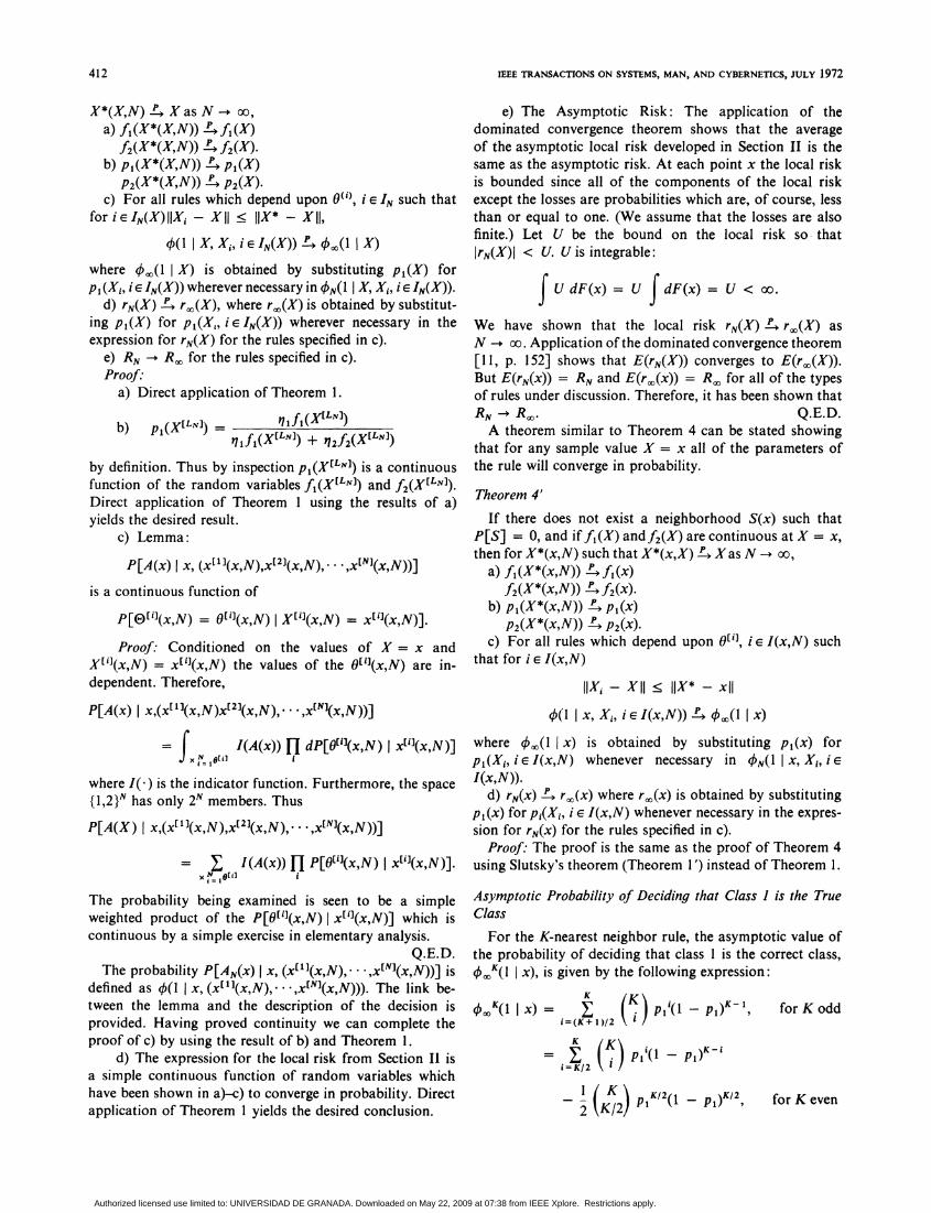
Fig. 5. Comparison of q(1 x) and local risk as function of p1(x)when losses are zero or one and number of preclassified samples islarge. K = 1, 2.

where Pi = p1(x). The probability O.K(1 x) is simply theprobability that more than one-half of the K-nearest pre-classified samples will be from class 1 when the probabilityof one of the samples being from class 1 is p1(x). Ties arebroken randomly.For the modified K-nearest neighbor rule, the probability

of deciding that class 1 is the correct class 0oKM(1 x) is

O. (1 I x) = plqoo (1 x)P1 K,(1 x) + (1 - pOO( - p0K(1 x))

00K( 1 I x)00 (1 x) [(1 l- )/PI](, - X(K(1Ix))

Applying the K-nearest neighbor rule to each of the pre-classified samples results in a probability equal to q5K thata sample from class 1 is retained. The probability that asample is from class 1 is p1(x). Normalizing by the prob-ability that the sample was retained regardless of its classyields the probability that any of the nearby preclassifiedsamples is from class 1, given that it is retained. In par-ticular, this probability applies to the nearest remainingneighbor to the sample to be classified.The asymptotic local risk is obtained by substituting one

of the expressions for 4(1 x) in the expression for thelocal risk in Section I. From Section I

r(x) = L(2 l)pl(x)(l - 4(l x))

+ L(1 2)(1 -p,(x))4(l x).

The comparison of the probabilities of deciding that asample is from class 1 as a function of p1(x) and the com-parison of the local risk as a function of p1(x) are shown inFigs. 5-10. Several facts should be noted from the com-parison.

1) The performance of the K-nearest neighbor rule whenK is even is the same as the performance of the K-nearest

BAYES-- 1-NEAREST NEIGHBOR

--- K-NEAREST NEIGHBOR-- -- MODIFIED K-NEAREST NEIGHBOR

0 O 0.2 0.4 0.6 0.8 1.0P1(X)

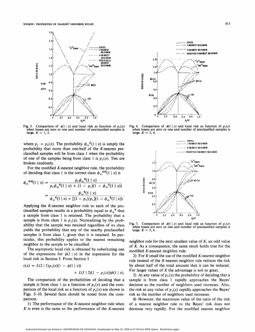
Fig. 6. Comparison of 0(1 x) and local risk as function of p1(x)when losses are zero or one and number of preclassified samples islarge. K = 3, 4.

L^

0Ot0!R

BAYES1-NEAREST NEIGHBOR

-- K-NEAREST NEIGHBOR

- MODIFIED K-NEAREST NEIGHBOR

0.80(1 Ix)

0.6

RISK X

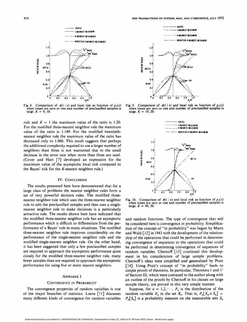
P1i)Fig. 7. Comparison of q(1 x) and local risk as function of p1(x)when losses are zero or one and number of preclassified samples islarge. K = 5, 6.

neighbor rule for the next smallest value of K, an odd valueof K. As a consequence, the same result holds true for themodified K-nearest neighbor rule.

2) For K small the use of the modified K-nearest neighborrule instead of the K-nearest neighbor rule reduces the riskby about half of the total amount that it can be reduced.For larger values of K the advantage is not so great.

3) At any value ofp1(x) the probability of deciding that asample is from class 1 rapidly approaches the Bayes'decision as the number of neighbors used increases. Also,the risk at any value of p1(x) rapidly approaches the Bayes'risk as the number of neighbors used increases.

4) However, the maximum value of the ratio of the riskof a nearest neighbor rule to the Bayes' risk does notdecrease very rapidly. For the modified nearest neighbor

413



BAYES-- 1-NEAREST NEIGHBOR

- --- K-NEAREST NEIGHBORS

MUSIL KaREST Ner.I

Lob*11

RIl

-M-- ODIFIED K-EREST NEI

1.0 ,_- _ ,-__-Rr- BayesI. 02 /,-^ rK/r Bt

///SK~~~ ~~~~~~ X aye

0.1P

0.6

0.4 rj'x\

0.2// /

00 0.2 0.4 0.6 0.18 1.0

IGHBORS

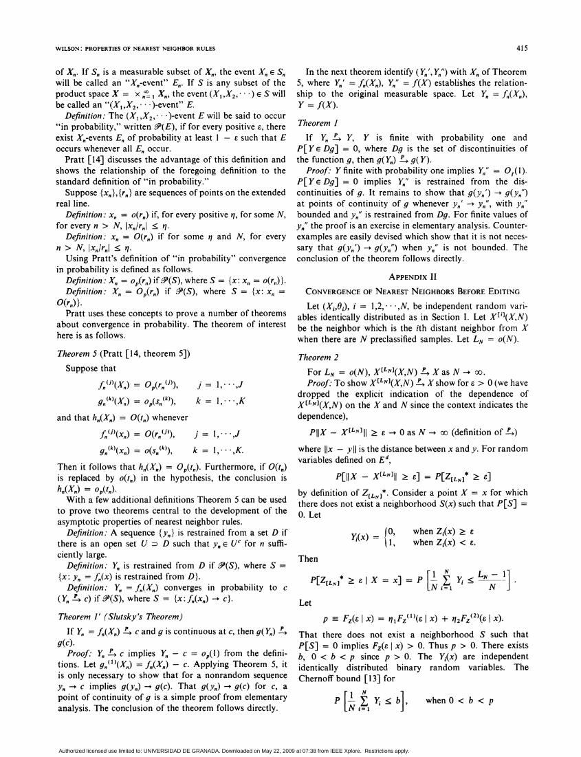
Fig. 8. Comparison of #(l x) and local risk as function of p1(x)when losses are zero or one and number of preclassified samples islarge. K = 9, 10.

4A

I-

z

BAYES- I-NEAREST NEIGHBOR

-- - - K-NEAREST NEIGHBOR

--- - MODIFIED K-NEAREST NEIGHBOR

P1i X

Fig. 9. Comparison of O(1 x) and local risk as function of pl(x)when losses are zero or one and number of preclassified samples islarge. K = 19, 20.

rule and K = I the maximum value of the ratio is 1.20.For the modified three-nearest neighbor rule the maximumvalue of the ratio is 1.149. For the modified twentieth-nearest neighbor rule the maximum value of the ratio hasdecreased only to 1.066. This result suggests that perhapsthe additional complexity required to use a larger number ofneighbors than three is not warranted due to the smalldecrease in the error rate when more than three are used.(Cover and Hart [7] developed an expression for themaximum value of the asymptotic local risk compared tothe Bayes' risk for the K-nearest neighbor rule.)

IV. CONCLUSIONS

The results presented here have demonstrated that for alarge class of problems the nearest neighbor rules form aset of very powerful decision rules. The modified three-nearest neighbor rule which uses the three-nearest neighborrule to edit the preclassified samples and then uses a single-nearest neighbor rule to make decisions is a particularlyattractive rule. The results shown here have indicated thatthe modified three-nearest neighbor rule has an asymptoticperformance which is difficult to differentiate from the per-formance of a Bayes' rule in many situations. The modifiedthree-nearest neighbor rule improves considerably on theperformance of the single-nearest neighbor rule and themodified single-nearest neighbor rule. On the other hand,it has been suggested that only a few preclassified samplesare required to approach the asymptotic performance quiteclosely for the modified three-nearest neighbor rule, manyfewer samples than are required to approach the asymptoticperformance for using five or more nearest neighbors.

APPENDIX I

CONVERGENCE IN PROBABILITY

The convergence properties of random variables is oneof the major branches of statistics. Loeve [11] discussesmany different kinds of convergence for random variables

BAYES-1-NEAREST NEIGHBOR

- - - - K-NEAREST NEIGHBOR-- - MODIFIED K-NEAREST NEIGHBOR

'A

0!i

I=

0.6 0.8 1.P1iX

Fig. 10. Comparison of O(I x) and local risk as function of pl(x)when losses are zero or one and number of preclassified samples islarge. K = 49, 50.

and random functions. The type of convergence that willbe considered here is convergence in probability. Simplifica-tion of the concept of "in probability" was begun by Mannand Wald [ 12] in 1943 with the development of the relation-ship of the operations that could be performed in determin-ing convergence of sequences to the operations that couldbe performed in determining convergence of sequences ofrandom variables. Chernoff [13] continued this develop-ment in his consideration of large sample problems.Chernoff's ideas were simplified and generalized by Pratt[14]. Using Pratt's concept of "in probability" leads tosimple proofs of theorems. In particular, Theorems 1 and 1'of Section III, which were conveyed to the author along withan outline of the proofs by Chernoff in his classes on largesample theory, are proved in this very simple manner.

Suppose, for n = 1,2, , Pn is the distribution of therandom variable Xn in the set X". That is, Pn[Xn e Sn] =P,[S,] is a probability measure on the measurable sets Sn

414



of X,. If S, is a measurable subset of X", the event X, E Snwill be called an "X,-event" E, If S is any subset of theproduct space X = x n I X,, the event (X1,X2, ) S willbe called an "(X1,x2,X2 )-event" E.

Definition: The (X1,X2,. )-event E will be said to occur"in probability," written .4(E), if for every positive e, thereexist X,-events En of probability at least I - E such that Eoccurs whenever all En occur.

Pratt [14] discusses the advantage of this definition andshows the relationship of the foregoing definition to thestandard definition of "in probability."

Suppose {x.},{r.} are sequences of points on the extendedreal line.

Definition: xn = o(r,) if, for every positive i, for some N,for every n > N, IxI/r,l < t1.

Definition: x = O(r") if for some q and N, for everyn > N, Ixn,/rnl < 1

Using Pratt's definition of "in probability" convergencein probability is defined as follows.

Definition: Xn = op(rn) if Y(S), where S = {x: xn = o(rj).}Definition: X. = Op(r,) if Y(S), where S = {x: xn =

O(r)}.Pratt uses these concepts to prove a number of theorems

about convergence in probability. The theorem of interesthere is as follows.

In the next theorem identify (Y,', Y") with Xn of Theorem5, where Y,' = f.(X.), Yn" = f(X) establishes the relation-ship to the original measurable space. Let Y, = f,(X,,),Y = f(X).

Theorem 1

If Y,, A Y, Y is finite with probability one andP[YE Dg] = 0, where Dg is the set of discontinuities ofthe function 9, then g(Y,) A g(Y).

Proof: Y finite with probability one implies Y,," = °rmlP[Ye Dg] = 0 implies Y," is restrained from the dis-continuities of g. It remains to show that g(yn') -+ g(yn")at points of continuity of g whenever y,,' -- y,,", with y,"bounded and Yn," is restrained from Dg. For finite values ofYn" the proof is an exercise in elementary analysis. Counter-examples are easily devised which show that it is not neces-sary that g(yn') -. g(yn") when y,," is not bounded. Theconclusion of the theorem follows directly.

APPENDIX II

CONVERGENCE OF NEAREST NEIGHBORS BEFORE EDITING

Let (X1,Oj), i = 1,2,* ,N, be independent random vari-ables identically distributed as in Section I. Let XE'3(X,N)be the neighbor which is the ith distant neighbor from Xwhen there are N preclassified samples. Let LN = o(N).

j=1, ,J

k I, ,K

j= 1, ,J

"(k)( = o(Sn(k)), k = 1, * ,K.

Then it follows that h.(X,) = Op(tn). Furthermore, if O(tj)is replaced by o(tn) in the hypothesis, the conclusion ish.(X.) = op(tn).With a few additional definitions Theorem 5 can be used

to prove two theorems central to the development of theasymptotic properties of nearest neighbor rules.

Definition: A sequence {y,} is restrained from a set D ifthere is an open set U v D such that yn E U' for n suffi-ciently large.

Definition: Y,, is restrained from D if p(S), where S =

{x: yn = f"(x) is restrained from D}.Definition: Y,, = fn(Xn) converges in probability to c

(Yn c) if 2P(S), where S = {x:f(x,) -4 c}.

Theorem I' (Slutsky's Theorem)

If Yn = fj(X") c and g is continuous at c, then g(Y,) p

g(c).Proof: Yn c implies Yn- c = op(l) from the defini-

tions. Let gn"l(Xn) =-J(Xn) - c. Applying Theorem 5, itis only necessary to show that for a nonrandom sequence

y- c implies g(y,) -4 g(c). That g(y.) -4 g(c) for c, a

point of continuity of g is a simple proof from elementaryanalysis. The conclusion of the theorem follows directly.

Theorem 2

For LN = o(N), X[LN](X,N) X as N -+

Proof: To show X[LNI(X,N) X show for E> 0 (we havedropped the explicit indication of the dependence ofX(LN](X,N) on the X and N since the context indicates thedependence),

PIIX X[LN]II -2 0 as N oo (definition of

where llx - ylI is the distance between x and y. For randomvariables defined on Ed,

P[IIX - X[LNII E] = P[Z[LN]* E]

by definition of Z[LN]*. Consider a point X = x for whichthere does not exist a neighborhood S(x) such that P[S] =

0. Let

Y , when Zi(x) s

(1, when Zi(x) < E.

Then

P[Z( P[iN

LN 1P[Z[LN] >- E X = X] = P [N E < N ]v

Let

P FZ(E X) = q1Fz(1'(8 X) + 12FZ(2)(6 | X).

That there does not exist a neighborhood S such thatP[S] = 0 implies FZ(£ x) > 0. Thus p > 0. There existsb, 0 < b < p since p > 0. The Yi(x) are independentidentically distributed binary random variables. TheChernoff bound [13] for

[N < b] when O< b < p

Theorem 5 (Pratt [14, theorem 5])Suppose that

fn(j(Xn) = °p(rn ())sgn(k)(Xn) = op(Sn (k)),

and that hn(Xn) = O(tj) whenever

fn(j(Xn) = 0(rn (i)),

415



has been developed in [12, p. 102]. This reference shows

p [1N Yi < b] . exp [-N(Tp(b) - H(b))]

where

Tp(b) = -b In p - (I -b) In (I - p)

H(b) = -b In p - (I -b) In (I - b).

Both Tp(b) and H(b) are well-known functions. It is knownthat Tp(b) - H(b) . 0. (See [12].) Since LNIN -. 0, for Nlarger than some No,

LN-1 < b.N

Therefore,

[ NE LN- I] _ Y . ]

for N greater than No. But

exp [-N(Tp(b) - H(b))] -O 0 as N -o.

Therefore,

p tEY.< L nIOasN uo

We have shown that for a sample value X = x, thenearest neighbor converges. It remains to show that therandom variable X has this property with probability one.We shall do this by showing that the set T of points whichdo not have this property has probability zero.

Let S(x,r.) be a sphere of radius rx centered at x, whererx is a rational number. Let T be the set of all x for whichthere exists a rational number rx sufficiently small thatP[S(x,rx)] = 0. The space Ed is certainly a separable space.From the definition of separability of Ed there exists acountable dense subset of A of Ed. For each x E T, thereexists a(x) E A such that a(x) E S(x,rx/3) since A is dense.By a simple geometric argument, there is a sphere centeredat a(x) with radius rx/2 which is strictly contained in theoriginal sphere S(x,rx) and which contains x. ThusP[S(a(x),rx/2)] = 0.The possibly uncountable set T is contained in the

countable union of spheres Ux TS(a(x),rx/2). The prob-ability of the countable union of sets of probability zero iszero. Since T c UXETS(a(x),rX/2), P[T] = 0, as was tobe shown.

APPENDIX III

CONVERGENCE OF NEAREST NEIGHBOR AFTER EDITINGLet (Xi,O,), i = 1,2, ,N, be independent random vari-

ables identically distributed as in Section I. Let (Xi,Oi) beedited as for the modified nearest neighbor rule. That is,

I) find the K-nearest neighbors to Xi among

{XX,X2, * * * ,X - I *Xi + I I* *XN }

2) find the class 0 associated with the largest number ofpoints among the K-nearest neighbors, breaking ties ran-domly when they occur;

3) edit the set {(Xj,Oj)} by deleting (Xi,Oi) whenever Oidoes not agree with the largest number of K-nearestneighbors as determined in the preceding.

Let there be M classes, m = 1,2, X,M. In particular,consider M = 2. (The proof is general enough to cover anyfinite value of M, but for consistency with the remainder ofthe paper M is considered to be 2.) Then

M

f(x) = S llmfm(X)m= 1

Pm(X) = P(O = m X = x) = uZmfm(X)f(x)Let XEK 1](xo,N) be the nearest neighbor to xo after editinghas been performed as outlined in the foregoing.

Theorem 3

If P[Xe Dfm] = 0, m = 1,2, *,M, where Dfm is the setof discontinuities offm(x), then XEKI1](X,N) P.-÷ Xas N o.

Proof: The proof is carried out by first examining pointsxo such that the fm(x) are continuous at xo and f(xo) > 0.For these points the following statements are proved.

I) There is anfsuch thatf(x) . f > 0 for all x lyingwithin a hypersphere of radius e centered at xo.

2) N"2 nonintersecting hyperspheres of radius e/2N i/2dcan be placed within the hypersphere of radius E centeredat xO.

3) As N grows large, the probability that a samplepoint may be found within a hypersphere of radius &I4N 1/2dconcentric to each of the hyperspheres of radius 8I2Ni/2dfor all N"I2 such spheres approaches one. (The fact thatN1/2 may not be an integer will be ignored since it makesno difference to the proof, and the details necessary to findan integer near to N'i2 will obscure an already complicatedproblem.)

4) As N grows large, the probability that at least Kneighbors to such a sample point are located within a radiusEI4NIl'2d of the sample point approaches one.

5) When the K neighbors of one sample point arewithin a hypersphere not intersecting a similar hyperspherecontaining another sample point with its K neighbors, theprobability of retention in the edited set is independent forthe two sample points.

6) As N grows large, the probability of at least onepoint being retained in the edited set approaches one.

7) Finally, the set of points which do not have thisproperty is shown to have probability zero.

Details of Proof: (In what follows XEK'1 will be used forXEK(I](xo,N) and XEK['I(X,N) depending upon the context.)From the definition of convergence in probability XEK[1] P

xo whenever for every E > 0

P[IXEK'1 - xo1 > E] - 0 as N -. oO.

1) The continuity Offm(x), m = 1,2, ,M implies thatM

f(x) = E tlmfm(X)m I

is continuous. Also, pm(x) is continuous since pm(x) is asimple continuous function offm(x) and f(x). (The proof istrivial.) Continuity implies that for every E > 0 there exists

416


417WILSON: PROPERTIES OF NEAREST NEIGHBOR RULES

6 > 0 such that for m = 1,2, *M,

Ifm(x) -fm(X)I < E, whenever Ix - xol < am

Pm(x) -Pm(xo)I < E, whenever Ix - xol < 3M+m

If(X) -f(x)I < £, whenever Ix - xol < 32M+1lSelect 3 = min(61,62,- *,32M+1) Then whenever Ix-xo <3, all of the preceding quantities are less than E. Select Esuch that 0 < E <f(xo) and 0 < E < 1/2M. This selec-tion can be done since f(xo) and 1/2M are positive. Letf = f(x0) -~E. Then Ifl = f > 0 since E < f(xo). ButIf(x) - f(xo)I < E whenever Ix - xol < 3 implies thatf(x) > f whenever Ix - xol < 3. Thus f> 0 is a lowerbound on f(x) whenever Ix - xol < 3. Similarly, =f(x0) + E is an upper bound. Since

IXEK[ ] - XOI > E, E > 3

implies that

IXEK"1] - XOI . e

when E < 3, proving that

P[IXEK"1 XOI2>] -O 0 as N - oo

for every E such that 0 < E < 3 is adequate to prove that

P[IXEK['] - XOI > E] -O 0 as N -- oo

for any E. The proof is continued on that basis.

2) The region Ix - xol < E defines a hypersphere witha volume in d dimensions of

id/2 dVd(E) =E.r'(d/2 + 1)6

Lemma: At least N1/2 nonintersecting hyperspheres ofradius eI2N 1/2d can be placed within a hypersphere ofradius E.

Proof: When as many nonintersecting hyperspheres ascan be packed in randomly have been placed in the hyper-sphere of radius E, there is no point in the E-radius hyper-sphere such that a small hypersphere cannot be found withina distance equal to the radius of the small sphere. If therewere such a point, another small hypersphere could beplaced within the large one by centering a new small hyper-sphere at the point so located. But if there is no point suchthat a small hypersphere cannot be found within a distanceequal to the radius of the small hypersphere, then con-centric spheres having twice the radius of the small sphereswill cover all of the points of the large hypersphere. Thesedouble-radius hyperspheres may be intersecting. However,the total volume covered by the double-radius hyperspherescannot be more than the sum of the volumes of each of theindividual double-radius hyperspheres. The sum of thevolumes of N1/2 hyperspheres of radius 1/N1/2d is

N 1/2 ____d/2 ( Ed d/26d

r(d/2 + 1) \N1/2d = F(d/2 + 1)

The last quantity is identified as the volume of the hyper-sphere of radius 6. ,Thus N1/2 hyperspheres of radiusE/N 1/2d have a combined volume at most equal to the

volume of the hypersphere of radius £, and at least N112hyperspheres of radius s12N1/2d can be placed within thehypersphere of radius E. Q.E.D.

Let U(j) = 0 when there is not a point Xi in the hyper-sphere with radius e/4Nl12d concentric to the jth hyper-sphere of radius sI2Nl/2d. Let U(j) = 1 when there is apoint in the hypersphere. When U(j) = 1 select one of thepoints within the hypersphere of radius &14N1/2d, and letthat point be X(i). Let

,

Yi(j) =

1,

when Xi - X /

when Xi - X < 1

Let E1 = 1 whenever

a) for all j, U(i) = 1;b) for all j, EN= 1 Yi(i) > K + 1; andc) at least one X(i) has an associated O(i) which agrees

with the largest number of the K-nearest neighborsto X(i.

Let E1 = 0 otherwise. When El = I at least one point isretained in the hypersphere of radius E after the editingprocess. (There is an i for which Xi = X(i). For that i,Yj(j) = 1, but X(i) is not one of the K-nearest neighbors toX(j) used in the editing process. Thus it is required that

I Y1(j) > K + I in order that the K-nearest neighborsto X(j) lie within a radius E/4NlI2d of the point X(j).)

Also, when

a) for all j, U(j) = 1; andb) for allj, _ IY(j) > K + 1

none of the K neighbors used in editing one point X(j) isused in editing any other point X(i ) since the conditions onU(i) and the sum of the Y1(i) imply that at least K of thenearest neighbors to each point X(i) lie within the hyper-spheres of radius c/2NlI2d which are nonintersecting.

3) Developing inequalities and using them in the proof:

P[IXEK['] - XOI . 6] < P[E1 = 0]since the one event implies the other. Continuing:

P[E1 = 0] = P[E1 = 0 for allj, UU) = 1]

P[for allj, U(i) = 1]

+ P[E1 = 0 1 for some j, U(i) = 0]

P[for somej, UO) = 0]< P[E1 = 0 1 for all j, U(i) = 1]

+ P[for somej, U(i) = 0]

since probabilities are less than or equal to one.Lemma:

P[for some j, U() = 0] -O 0 as N oo.

Proof:= 0]= i- SjE4N/)f()xN

P[U Mj = O] I f-f(x) dxS(j,E4NI /2d)


IEEE TRANSACTIONS ON SYSTEMS, MAN, AND CYBERNEnCS, JULY 1972

where S(j, c/4Nl/2d) indicates that the integral is taken overthe volume of a hypersphere with radius eI4Nl/2d con-centric with the jth hypersphere of radius 612N 1/2d(P[U(j) = 0] is the probability that no sample lies withinthe jth hypersphere from the definition of U(J)). This istrue since each of N independent samples Xi may be withinthe specified volume with equal probability. But f(x) 2 fin the region occupied by the hypersphere implies that

f(x) dx . T f dx.S(j,el4NI1 2d )fJ,£/4N1/2d)

Thus

( - ff(x) dx) < (1 - f dx)

= (1 - fv(, )d4N 1/2d

where Vd(a) is the volume of a hypersphere with radius a.Then

P[for some j, U(j) = 0]= P[either U(') - 0 or U = 0 or * or U(NI/2) = 0]

N112

< E P[U(j) = 0]j=l

. N'/ (1 -I Vd (4N 1/2d))

But

7rd/26d(4N /2d) =J(d/2 + 1)4dN/2

Let

,td/2EdJ(d/2 + 1)4d

Note that Cd > 0 since it is the product of strictly positivequantities:

N2[1/2 Cd Nand P[U(j) = O] < N 1 -

and

N 12 (i - Cdp N

N 1/2J

= exp ( In (N) + N In (I -N1/2))

= exp ( ln (N) + N ( _2 + (I)))

= 0(1) exp ({ In (N) - N/2cd)-+ 0 as N -+ oo.

Therefore, P[for somej, U(i) = 0] -O 0 as N oo.

Q.E.D.

4) Continuing with the main theorem and recallingthat ', = 1 Yi(i) . K + 1 implies that K neighbors lie withinthe hypersphere of radius sI4Nl/2d centered at X(i),P[El = 0 1 for all j, U (i) = 1]

= P [E1 = Of for all j,

N

Y Yi(j) > K + 1 and for allj, U(J =i=1

-for a] y>lNp for all j, E Yi(J) > K + I for allj, U (J) =-

= 1

1]

1]

+ P [E1 = 0 1 for some j,

N

Yi() < K + l and for all j, U(U) = Ii= 1

* P [forsome]j, Y,(i) < K + I for allj, U(i) = 1]

. P [El = 0 for all j,

N

Yi(j) K + 1 and for allj, U) = 1]i= 1J

+ P [for somej, Y5(j) < K + I for allj, U(3) = 1]

since probabilities are less than or equal to one.Lemma:

NP for some, (J) < K + 1I for all j, U(J) = I

i= 1I

0 as N -- oo.

Proof: Note that Y1(i) = 1 for the point which is x(i).Thus we must show that there are not K other points withina distance E/4Nl/2d of X to show that i = <K + 1. Note also that since Xi, i = 1,2,' ,N, are drawnindependently from one population, the Yi for one j arealso independent. Considering only one j,

P 1o < K + If U (j)I

Let

f(x) dxS(X(i),t14NI12d)

where S(X(j), s/4N1/2d) indicates that the integral is to betaken over the volume of a hypersphere with radiuse14Nl1l2d centered at X(j). p has an upper and a lower bound:

0< = f dx < p < P'(X(j),E/4Nl12d)

= I S(X(J),e d f dxS(X ( }),e14Nl12d)

418



since 0 < f f(x) < f for x such that Ix -xol < e.Evaluating

P = jf dx = fJdx = fVdK,2d)

and

p = f dx = f dx = f Vd (4j12d)For N large enough

0 < K+ 1 < P = idl2gdf < P = E(Yi(j))N - 1 - If(d/2 + l)4dNhI2< ,=EY)

except for the i for which Xi = X(i). Thus for N largeenough Chernoff's bound can be applied:

P[N_11 y (j) K + 1 U M = 1

< exp [-(N - 1) (Tp (N ) - H (NK ))1

where

Tp(a) = -alnp -(1 - a)ln(l -p)

H(a) -a In a - (1 - a) ln (1 - a).

Let7mdl2edf

F(d/2 + 1)4d

and Cd be similarly defined by substituting f for f in thedefinition. Using the upper and lower limits developed,

exp [-(N -1) (TP (N 1) (N 1))< exp (N - 1) {K (In (Cd) + l N -I

+ (1 N- 1) (ln(1 K N1

ln(1 K I)))]

Observing that for y > 0 and y small ln (1 - y) = -y +0(y2) and carrying out some algebra, we modify the lastexpression to

exp [-(N - 1) (T (Nl- 1) H(N- ))]

= 0(1) exp [K In (N) -N 1/2Cd]

Thus

P [ Y(j) < K + I I U=(j) 1]

< 0(1) exp [K ln (N) - N1/2Cd]

_ ~~NP for some j, Yi(i) < K + I I for every j, U (j)=

= P[ Yi(') < K + 1 or y(2) < K + 1 or *.or

,yiN"'2) < K + I I for all j, U() = 1]

N112

<- P[Y Yi(i) < K + 1 U (i) = 1]j=lN112 K

<- 0(1) exp - ln (N)-N12-Cd

= N112 0(1) exp [- ln (N) -N1/2Cd]

= 0(1) exp [K + 1ln (N) -N1/2Cd]

0 as N -+ oo.

Therefore,N

P for some j, , Yi(j) < K + 1 t for every j, U (i) =i= 1

-+ 0 as N -+ 0o.

Ii

).E.D.

5) Continuing with the main proof, let

when X() is retainedotherwise.

Let V = (V(1), V(2) .V(Nf12)_ ~~~~N

P [E1 = Olfor all j, Yy.(i) > K + 1L ~~~~~~~i= 1

and for allj, U(j) = I

= P[V = (0,0, * ,0) for all j, E Yj(j) > K + 1

and for all j, U(j) = 1].But under the conditioning all of the V(j) are independentsince each V(j) depends only on the values of 0 associatedwith sample points within the jth hypersphere of radiuss/2N1/2d, and none of these hyperspheres intersect anothersuch hypersphere. Therefore,

P[V = (0,0, ,0) for all j, E Yj(j) > K + 1

and for allj, U(j) = 1]N112

= l P[V(j) = 0 for all j, Y.(j) > K + 1j=1and for all j, U (j) = 1].

6) Lemma:

P[V(j)= 0 for all]j, Yi(j) > K + 1

and for allj, U(j) = 1] < 1 -, y > 0.

Proof: The lemma states that when there is a samplein every one of the j hyperspheres and when the K-nearestneighbors to each of the samples also lie within the respec-tive hyperspheres, the probability that X(j) is not retained

419

Q

VU) =L

05



is less than one. The equivalent statement that the prob-ability of retaining X(j) is greater than zero will be proved.

Let CG be the event that L Y.(j) > K + 1 and U(j) = 1.Also, let

E2(m) =

kO,

when the plurality of the K-nearest

neighbors is from class motherwise

andM

P[V(U) = 1 C] = P[V( = 1 C}m =1

and E2(m) = 1] * P[E2(m) = 1 C].

Let mi be the class that has the largest probability of havinga plurality. (Ties are broken randomly.) Then

P[Vj) = 1 Cj] P[V(J) = Cjand E2(iz) = 1] P[E2(M) = I CJ]

since the sum is a sum of positive quantities. But

P[EAfh) = 1 C] M.

Since probabilities sum to one, there are M classes, and ih

is the class with the greatest probability. Therefore,

P[V(U) = 1 Cj] P[V(M) = 1 C,

and E2(h) = 1]3-.But

P[E20h) = 1 Cj]

implies that for some x in the hypersphere of radiuss/4Nl/2d centered at X(j)

P,h(x) -P(O = m X = x) > M

since P[E2(mh) = 1 Cj] is an average of p,;(x). However,p,j(x) is a continuous function of x. In particular, theselection of a in step 1) guarantees

Ip,h(x) - ph(xo)lI

for Ix - xol < &.

Therefore, p,&(x(i)) > 0 since

Jp,h(x) PR(X j))l IPh(X) ph(xO) + p,m(XO) - Ah(XUN

< Ip,(x) -p,(xo)I + Ip,W(xO) - P,(x ('))

1 1 1

2M 2M M

Thus there exists a y > 0 such that

P[V(j) = 11 Cj and E2(Qh) = 1] My > 0

since this probability is an average of p,(X(J)) over thepossible values of x(i) and prn(x(i)) > 0. This implies

P[V() = 1 C3] My * = y > 0

M

and finallyP[V(J) = 0 Cj] < 1 - y. Q.E.D.

Completing the main proof by using the results of thelemmas,

P[V = (0,0, *,0) for all j, Ci]N1/2

= H P[V(J) = 0 c3]j= 1

N112< 17 (1 - y= (1 - ,)NI/2

j=1

0 as N -.

Combining all of the inequalities,

P[DXEKI] - xol > E]

. P[for some j, U(J) = 0]N

+ P for some j,N

< K + Il for all]j, U = 1]

N+ P V = (0,0, * ,O) for all j, YyU)

< K + land for allj, U() = 1]

0 as N -+oo

since each of the three components on the right approaches0 as N -- oo.

7) Finally, we must argue that the set of points forwhich the edited nearest neighbor does not converge to thesample to be classified has probability zero. The argumentis very similar to the argument of a theorem of Cover andHart [7]. We have shown that for point of continuity off(x) for which f(x) is greater than zero the edited nearestneighbor converges in probability. It remains to considerpoints for which f(x) is not continuous or for whichf(x) = 0. The set of discontinuities has measure zero byhypothesis. The set for whichf(x) = 0 is more complicated.

Let S(x,r.) be a sphere of radius r. centered at x, rx arational number. Let V be the set of all x such that theredoes not exist an rx sufficiently small that P[S(x,rx)] = 0,but for which f(x) = 0 and f(x) is continuous. For x E Vthe edited nearest neighbor converges in probability. Sincethe set of discontinuities off(x) has probability zero and xis a point of continuity of f(x), there must be a point twithin E/3 of the point x for which f(t) > 0 and which isa point of continuity off. If not, P[S(x,rx)] would be zerofor some rx small enough. If there remains a preclassifiedsample within a distance E/3 of the point t, there will be apreclassified sample within a distance e of the point x by asimple geometric argument. We have shown that for pointswith the property of the point t, the probability of therebeing a preclassified sample within an arbitrarily smalldistance e/3 approaches one as the number of preclassifiedsamples approaches infinity. Therefore, the probability that

420


IEEE TRANSACTIONS ON SYSTEMS, MAN, AND CYBERNETICS, VOL. SMC-2, NO. 3, JULY 1972

there will be at least one preclassified sample within adistance s of the point x approaches one as the number ofpreclassified samples approaches infinity. If at least onepreclassified sample is within s, then the nearest preclassifiedsample is within , and the nearest preclassified sample afterediting converges in probability to the point x.

Let T be the set of all x for which there exists an rxsufficiently small so that P[S(x,rx)] = 0. The set Thas prob-ability zero. Duplicating the argument of Theorem 2 webegin by observing that the space Ed is a separable space.From the definition of separability, there exists a countabledense subset A of Ed. For each x E T there exists a(x) E Asuch that a(x) e S(x,rJ/3) since A is dense. By a simplegeometric argument there is a sphere centered at a(x) withradius rJ/2 which is strictly contained in the original sphereS(x,rx) and which contains x. Thus P[S(a(x),rx/2)] = 0.The possibly uncountable set T is contained in the countableunion of spheres U x e T S(a(x), rx/2). The probability of thecountable union of sets of measure zero is zero. SinceT c UXET S(a(x), rx/2), P[T] = 0, as was to be shown.

ACKNOWLEDGMENT

The author is deeply indebted to Dr. T. Cover andDr. H. Chernoff for their many helpful suggestions andcareful review of the results presented in this paper.

REFERENCES[1] E. Fix and J. L. Hodges, Jr., "Discriminatory analysis, non-

parametric discrimination: consistency properties," U.S. AirForce Sch. Aviation Medicine, Randolf Field, Tex., Project21-49-004, Contract AF 41(128)-31, Rep. 4, Feb. 1951.

[2] G. Sebestyen, Decision-Making Processes in Pattern Recognition.New York: Macmillan, 1962.

[3] N. Nilsson, Learning Machines. New York: McGraw-Hill,1965.

[4] C. A. Rosen, "Pattern classification by adaptive machines,"Science, vol. 156, Apr. 7, 1967.

[5] G. Nagy, "State of the art in pattern recognition," Proc. IEEE,vol. 56, pp. 836-862, May 1968.

[6] Y. C. Ho and A. K. Agrawala, "On pattern classification al-gorithms-introduction and survey," IEEE Trans. Automat.Contr., vol. AC-13, pp. 676-690, Dec. 1968.

[7] T. M. Cover and P. E. Hart, "Nearest neighbor pattern classifica-tion," IEEE Trans. Inform. Theory, vol. IT-13, pp. 21-27, Jan.1967.

[8] A. W. Whitney and S. J. Dwyer, III, "Performance and imple-mentation of K-nearest neighbor decision rule with incorrectlyidentified training samples," in Proc. 4th Annu. Allerton Conf.Circuit and System Theory, 1966.

[9] T. M. Cover, in Methodologies ofPattern Recognition, S. Watanabe,Ed. New York: Academic Press, 1969.

[10] E. A. Patrick and F. P. Fischer, III, "A generalized k-nearestneighbor rule," Inform. Contr., vol. 16, pp. 128-152, Apr. 1970.

[11] M. Loeve, Probability Theory, 3rd ed. Princeton, N.J.: D. VanNostrand, 1963.

[12] H. B. Mann and A. Wald, "On stochastic limit and order relation-ships," Ann. Math. Statist., vol. 14, 1943.

[13] H. Chernoff, "Large sample theory: Parametric case," Ann.Math. Statist., vol. 27, 1956.

[14] J. Pratt, "On a general concept of 'in probability'," Ann. Math.Statist., vol. 30, June 1959.

[15] J. Wozencraft and I. Jacobs, Principles of Communication Engin-eering. New York: Wiley, 1965.

End Points, Complexity, and Visual IllusionsDAVID J. PARKER, STUDENT MEMBER, IEEE, AND DOUGLAS J. H. MOORE, MEMBER, IEEE

Abstract-One aspect of a new theory of feature perception is con-sidered. An algorithm is presented which can perceive and locate variousfeatures of a pattern by analyzing a statistic of the "chords" of thepattern. The procedure is illustrated by applying the algorithm to apattern containing the Muller-Lyer figures. In measuring the length ofthe figures it is found that the algorithm has a visual illusion. A machinecapable of executing the algorithm is described.

I. INTRODUCTIONA LARGE NUMBER of proposals for computers that,

in at least certain senses of the phrase, "recognizepatterns" have been published in the past ten years. In spiteof this the pattern recognition problem can still be said tobe in-its infancy. Levine [12], in his survey on featureextraction, stated that "the literature overwhelmingly con-centrates on the various aspects of classification," even

Manuscript received April 19, 1971; revised November 19, 1971.This work was supported by the Department of Supply.The authors are with the Department of Electrical Engineering,

University of Newcastle, Newcastle, New South Wales, 2308, Aus-tralia.

though David [4], in his review of the book by Sebestyen,raised the objection, "Is not the more significant part ofthe problem that of characterizing the world by a set ofproperties that provide the desired discrimination?" Itwould therefore seem that the problems of feature percep-tion and extraction must be solved before any headway canbe made with the pattern recognition problem. Nilsson [16],commenting on the subject of feature extraction, made thepoint that there exists no general theory which allows us tochoose what features are relevant for a particular problem.He also pointed out that the design of feature extractors isempirical and uses many ad hoc strategies. It would seemfrom these comments that a completely new approach tofeature extraction is necessary.Moore [13] described a theory of feature perception and

extraction. It was shown that the features of two-dimen-sional plane patterns could be perceived and extracted byanalyzing the statistics of the chords of a pattern. The typesof features that could be extracted included metric, angular,and topological structure. A two-dimensional retinal com-

421


Documents

Asymptotic Nearest Rules Using Data - UGRsci2s.ugr.es/keel/pdf/algorithm/articulo/1972-Wilson-IEEETSMC.pdf · rules and the nearest neighbor rules using edited preclassified samples