ASYMPTOTIC ANALYSIS OF THE BOUNDARY LAYERarnold/papers/bdlayer2.pdf · SIAM J. MATH. ANAL. c 1996 Society for Industrial and Applied Mathematics Vol. 27, No. 2, pp. 486{514, March

SIAM J. MATH. ANAL. c© 1996 Society for Industrial and Applied Mathematics

Vol. 27, No. 2, pp. 486–514, March 1996 009

ASYMPTOTIC ANALYSIS OF THE BOUNDARY LAYERFOR THE REISSNER–MINDLIN PLATE MODEL∗

DOUGLAS N. ARNOLD†

and RICHARD S. FALK‡

Abstract. We investigate the structure of the solution of the Reissner–Mindlin plate equations

in its dependence on the plate thickness in the cases of soft and hard clamped, soft and hard simplysupported, and traction free boundary conditions. For the transverse displacement, rotation, and

shear stress, we develop asymptotic expansions in powers of the plate thickness. These expansionsare uniform up to the boundary for the transverse displacement, but for the other variables there is a

boundary layer, which is stronger for the soft simply supported and traction-free plate and weaker for

the soft clamped plate than for the hard clamped and hard simply supported plate. We give rigorouserror bounds for the errors in the expansions in Sobolev norms. As an application, we derive new

regularity results for the solutions and new estimates for the difference between the Reissner–Mindlinsolution and the solution to the corresponding biharmonic model.

Key words. Reissner, Mindlin, plate, boundary layer

AMS(MOS) subject classifications. 73K10, 73K25

1. Introduction. The Reissner–Mindlin model for the bending of an isotropicelastic plate in equilibrium determines ω, the transverse displacement of the midplane,and φ, the rotation of fibers normal to the midplane, as the solution of the partialdifferential equations

−t3 div C E(φ)− λt (gradω − φ) = F ,

−λt div (gradω − φ) = G.

Here F is the applied couple per unit area, G is the applied transverse load densityper unit area, t is the plate thickness, λ = Ek/2(1 + ν) with E the Young’s modulus,ν the Poisson ratio, and k the shear correction factor, E(φ) is the symmetric part ofthe gradient of φ, and the fourth-order tensor C is defined by

CT = D [(1− ν)T + ν tr(T )I] , D =E

12(1− ν2),

for any 2 × 2 matrix T (I denotes the 2 × 2 identity matrix). These equations aresatisfied on the plane region Ω occupied by the midsection of the plate. In this paper,we investigate the dependence on the plate thickness of solutions to some boundaryvalue problems associated to these equations.

∗ Received by the editors March 10, 1993; accepted for publication (in revised form) August 2,

1994.†Department of Mathematics, Pennsylvania State University University Park, PA 16802. The

research of this author was supported by National Science Foundation grants DMS-86-01489, DMS-8902433, and DMS-9205300.

‡Department of Mathematics, Rutgers University, New Brunswick, NJ 08903. The research of

this author was supported by National Science Foundation grants DMS-87-03354, DMS-8902120, andDMS-9106051.

486

boundary layer for the reissner–mindlin plate 487

We consider various homogeneous boundary conditions of physical interest:

φ · n = φ · s = ω = 0 (hard clamped),(1.1)

φ · n = Ms(φ) = ω = 0 (soft clamped),(1.2)

Mn(φ) = φ · s = ω = 0 (hard simply supported),(1.3)

Mn(φ) = Ms(φ) = ω = 0 (soft simply supported),(1.4)

Mn(φ) = Ms(φ) = ∂ω/∂n− φ · n = 0 (free),(1.5)

in which n and s denote the unit normal and counterclockwise tangent vectors, re-spectively, and Mn(φ) := n · C E(φ)n, Ms(φ) := s · C E(φ)n. Each of the first fourboundary value problems admits a unique solution ω ∈ H1(Ω), φ ∈ H1(Ω) for anyF ∈ L2(Ω) and G ∈ L2(Ω). The existence theory for the free plate is slightly morecomplicated and will be discussed in §6.

We do not treat the Reissner–Mindlin model in its full generality. In addition tothe assumption of homogeneous boundary conditions, we shall assume that there isno applied couple, so F ≡ 0, and that the constitutive parameters E, ν, and k areindependent of t. It seems clear that the techniques developed here apply to moregeneral situations as well.

We also suppose that G = gt3, where the function g does not depend on t. This isa convenient normalization, which leads to φ and ω having a nonzero limit as t tends tozero. Given that the first differential equation and the boundary conditions are takento be homogeneous, this normalization is not restrictive. If G were to be proportionalto some other function h(t), we could make the change of dependent variables φ =t3φ/h(t), ω = t3ω/h(t) and the new variables would satisfy the Reissner–Mindlinequations with load proportional to t3.

With these assumptions, the Reissner–Mindlin equations become

−div C E(φ)− λt−2 (gradω − φ) = 0,(1.6)

−λt−2 div (gradω − φ) = g.(1.7)

After a similar normalization of the load, the biharmonic model for plate bendingmay be written

D∆2 ω0 = g in Ω,

and so its solution ω0 is independent of the plate thickness. In contrast, the solutionof the Reissner–Mindlin model exhibits a complex dependence on the plate thickness,which we investigate in the present paper. In previous work [1], we gave an analysisof the boundary layer for the Reissner–Mindlin model of hard clamped and hardsimply supported plates. There are many additional complications in the case of moregeneral boundary conditions, and so the analysis of [1] is not easily extended to thesoft simply supported and free plates, for example. In this paper, we analyze theboundary layer for all the boundary conditions mentioned above in a unified fashion.While the approach here is more complete, it is also simpler than that of [1] in anumber of ways. Thus the present paper essentially supersedes that one. We shallshow that the boundary layer is strongest for the soft simply supported and free plate,somewhat weaker for the clamped and hard simply supported plate, and weakest forthe soft clamped plate. In addition, we shall demonstrate that for the soft clamped

488 douglas n. arnold and richard s. falk

and hard simply supported plates, there is no boundary layer near a flat portion ofthe boundary.

We shall develop asymptotic expansions with respect to t for ω and φ (as wellas for other quantities associated with the solution such as the shear strain). Theexpansions take the forms

ω ∼ ω0 + tω1 + t2ω2 + · · · ,φ ∼ φ0 + χΦ0 + t(φ1 + χΦ1) + t2(φ2 + χΦ2) + · · · ,

where the interior expansion functions ωi and φi are independent of t and the boundarycorrectors Φi depend on t only through the quantity ρ/t, ρ being the distance of apoint of Ω from the boundary. More specifically,

Φi = Φi(ρ/t, θ),

where θ is a coordinate which roughly gives arc length parallel to the boundary (see§2), and the function Φi(η, θ) has the form of a polynomial with respect to η with coef-ficients depending smoothly on θ times exp(−

√12kη). Thus Φi represents a boundary-

layer function, which essentially lives in a strip of width t around the boundary. Fi-nally, χ is a cutoff function which is independent of t and identically equal to unity ina neighborhood of ∂Ω.

After some preliminary material in §2, we construct the terms of the asymptoticexpansions in §3 (for all of the boundary conditions except for those of the free plate,which is treated in §6). Then, in the following two sections, we justify the expansionsrigorously in the case of the soft simply supported plate, proving a priori boundsfor the terms of the expansions in §4 and performing the error analysis in §5. Thisanalysis can be adapted easily to the cases of hard simply supported and hard and softclamped plates, and somewhat less easily to the case of the free plate. The necessarymodifications are discussed in § 6. To make it easier for the reader to follow some of thecomputations performed in the derivation and analysis of the asymptotic expansions,we have included in an appendix a summary of the main formulas we have used. Inthe remainder of this introduction, we summarize some of the principal results.

For each of the boundary conditions, ω0 is the solution of the biharmonic equation

D∆2 ω0 = g

determined by appropriate boundary conditions, namely

ω0 =∂ω0

∂n= 0

for the hard and soft clamped plates,

ω0 = (1− ν)∂2ω0

∂n2 + ν∆ω0 = 0

for the hard and soft simply supported plates, and

(1− ν)∂2ω0

∂n2 + ν∆ω0 =∂∆ω0

∂n+ (1− ν)

∂

∂s

(∂2ω0

∂s∂n− κ∂ω0

∂s

)= 0

for the free plate. In the last expression, κ denotes the curvature of the boundary.


The next term in the expansion of the transverse displacement, ω1, vanishes forthe hard and soft clamped plates and the hard simply supported plate but not forthe soft simply supported or free plates. In these cases, it is the solution of thehomogeneous biharmonic problem

∆2 ω1 = 0 in Ω

with the inhomogeneous boundary conditions

ω1 = 0, (1− ν)∂2ω1

∂n2 + ν∆ω1 = − (1− ν)√3k

∂3ω0

∂s2∂n

for the soft simply supported plate and

(1− ν)∂2ω1

∂n2 + ν∆ω1 =1√3k∂∆ω0

∂n,

∂∆ω1

∂n+ (1− ν)

∂

∂s

(∂2ω1


∂s

)= − (1− ν)√

3k∂

∂s

(κ

[∂2ω0


∂s

])for the free plate.

Note that the expansions for the soft and hard simply supported plates differalready in the term ω1. For the soft and hard clamped plates the terms ω0, ω1, andω2 all agree, but ω3 = 0 for the soft clamped plate and is generally nonzero for thehard clamped plate.

Turning to the expansion of φ, we find that in all five cases that φ0 = gradω0

and φ1 = gradω1 while φ2 − gradω2 = λ−1D∆ω0, which is never zero (except inthe trivial case g ≡ 0). For the boundary correctors, we find that Φ0 vanishes in allfive cases. For the soft simply supported and free plates,

Φ1(η, θ) = − 1√3k

exp(−√

12kη)(∂2ω0


∂s

)(0, θ)s.

For the hard clamped and hard simply supported plate, Φ1 vanishes as well as Φ0 andwe have

Φ2(η, θ) = − 16k(1− ν)

exp(−√

12kη)∂

∂s∆ω0(0, θ)s

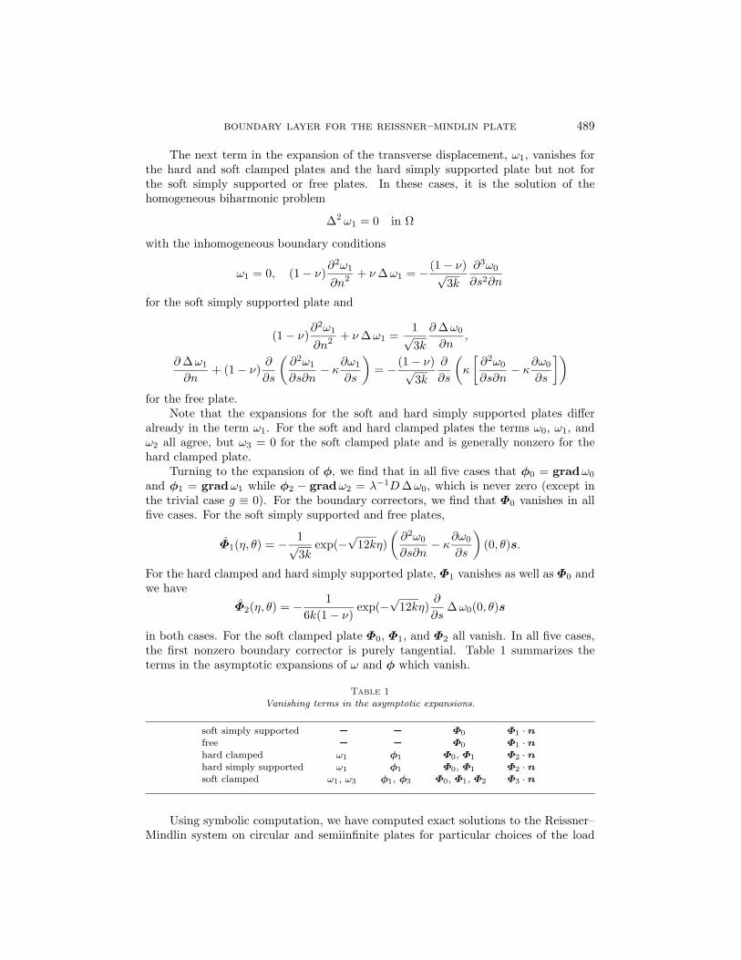
in both cases. For the soft clamped plate Φ0, Φ1, and Φ2 all vanish. In all five cases,the first nonzero boundary corrector is purely tangential. Table 1 summarizes theterms in the asymptotic expansions of ω and φ which vanish.

Table 1

Vanishing terms in the asymptotic expansions.

soft simply supported Φ0 Φ1 · nfree Φ0 Φ1 · nhard clamped ω1 φ1 Φ0, Φ1 Φ2 · nhard simply supported ω1 φ1 Φ0, Φ1 Φ2 · nsoft clamped ω1, ω3 φ1, φ3 Φ0, Φ1, Φ2 Φ3 · n

Using symbolic computation, we have computed exact solutions to the Reissner–Mindlin system on circular and semiinfinite plates for particular choices of the load


function g, and have explicitly computed the asymptotic expansions of ω and φthrough terms of order 6. These computations verify the sharpness of the resultsin this paper in that no terms of the expansions vanish except those given in thetable. These results have been reported in [2].

As an application of our asymptotic analysis, we can determine the asymptoticbehavior of Sobolev norms of solutions of the Reissner–Mindlin system. Supposingthat g is sufficiently smooth, we have the following estimates, valid for both the softsimply supported and free plate, in which the constant C depends on g, Ω, and theelastic constants but is independent of t. Here ‖ · ‖s and | · |s denote the norms inthe Sobolev spaces Hs(Ω) and Hs(∂Ω) (see §2).

The transverse displacement ω and all of its derivatives are bounded uniformlyin t, that is,

‖ω‖s ≤ C, s ∈ R,

but the regularity of the rotation φ is limited by the boundary layer. For example,for the soft simply supported and free plates, we have

‖φ‖s ≤ Ctmin(0,3/2−s), s ∈ R,

so derivatives of order greater than 1 will generally tend to infinity in L2 as t→ 0.The quantity ζ := t−2(gradω − φ), which is proportional to the shear strain, is

often of interest. From the above expansions, we get

ζ ∼ −t−1χΦ1 + (gradω2 − φ2 − χΦ2) + · · · ,

so it has a stronger boundary layer. Indeed, for the soft simply supported and freeplates, ζ is not uniformly bounded in L2, or even in Hs for s > −1/2:

‖ζ‖s ≤ Ctmin(0,−1/2−s), s ∈ R.

The corresponding estimates for the hard clamped and hard simply supportedplates are

‖φ‖s ≤ Ctmin(0,5/2−s), s ∈ R, ‖ζ‖s ≤ Ctmin(0,1/2−s), s ∈ R,

and for the soft clamped plate

‖φ‖s ≤ Ctmin(0,7/2−s), s ∈ R, ‖ζ‖s ≤ Ctmin(0,3/2−s), s ∈ R.

Of course, the boundary layer does not limit the regularity of φ or ζ at a positivedistance from ∂Ω nor does it affect the smoothness of their restrictions to ∂Ω. Thus

‖φ‖Hs(Ωc) + |φ|s + ‖ζ‖Hs(Ωc) + |ζ|s ≤ C, s ∈ R,

for any compact subdomain Ωc of Ω.In the limit as t → 0, the variables ω and φ tend in L2 to the leading terms

of their asymptotic expansions. The number of derivatives which converge and therate of convergence may be determined by examining the first neglected interior andboundary terms of the expansions. For any s ∈ R, we get for the soft simply supportedand free plate

‖ω − ω0‖s ≤ Ct, ‖φ− φ0‖s ≤ Ctmin(1,3/2−s).

Note that the rate of convergence for φ depends on the Sobolev norm under consid-eration. For each of the variables, taking more terms from the expansion increases


the rate of convergence and taking sufficiently many terms in the expansions gives ap-proximation of any desired algebraic order of convergence in t in any desired Sobolevspace (provided g is sufficiently regular). For example,

‖ω − ω0 − tω1‖s ≤ Ct2, ‖φ− φ0 − t(φ1 + χΦ1)‖s ≤ Ctmin(2,5/2−s).

For the hard clamped and hard simply supported plates, the analogous results are

‖ω − ω0‖s ≤ Ct2, ‖φ− φ0‖s ≤ Ctmin(2,5/2−s),

‖ω − ω0 − t2ω2‖s ≤ Ct3, ‖φ− φ0 − t2(φ2 + χΦ2)‖s ≤ Ctmin(3,7/2−s).

For the soft clamped plate,

‖ω − ω0‖s ≤ Ct2, ‖φ− φ0‖s ≤ Ctmin(2,7/2−s),

‖ω − ω0 − t2ω2‖s ≤ Ct3, ‖φ− φ0 − t2φ2‖s ≤ Ctmin(3,7/2−s).

It is also possible to use our asymptotic expansions to derive estimates in functionspaces other than Hs. The technique for doing this is described in [1]. Furtherreferences for the Reissner–Mindlin model and its boundary-layer behavior can alsobe found there. Many of the results in this paper were described without proof in [2],where explicit illustrations of the theory are constructed.

2. Notation and preliminaries. The letter C denotes a generic constant, notnecessarily the same in each occurrence. We assume that Ω is a smooth, bounded, andsimply connected domain in R2. The L2(Ω) and L2(∂Ω) inner products are denoted by( · , · ) and 〈 · , · 〉, respectively. We also use the usual L2-based Sobolev spaces Hs(Ω)and Hs(∂Ω), real s ≥ 0, with norms denoted by ‖ · ‖s and | · |s. When the domainargument is omitted, L2 and Hs refer to L2(Ω) and Hs(Ω). The space Hs = Hs(Ω)is the closure of C∞0 in Hs. The interpolation inequality

(2.1) ‖g‖us+v ≤ C‖g‖u−vs ‖g‖vs+u, s ≥ 0, u ≥ v ≥ 0,

holds. If g ∈ L2 and ∆−1 g denotes the unique function in H2 ∩ H1 whose Laplacianis equal to g, then

C−1‖∆−1 g‖s+2 ≤ ‖g‖s ≤ C‖∆−1 g‖s+2, s ≥ 0,

where the constant C may depend on s and Ω but not on g. In other words,g 7→ ‖∆−1 g‖s+2 defines an equivalent norm on Hs for s ≥ 0. We also define somenegatively indexed norms which maintain this equivalence:

‖g‖s := ‖∆−1 g‖s+2, −2 ≤ s < 0.

For s = −1, this is equivalent to the norm in the dual space of H1. For s = −2, itis equivalent to the norm in the dual space of H2 ∩ H1. With this definition, (2.1)holds for s ≥ −2. We shall make frequent use of this fact to bound sums of the form∑ni=0 t

i‖g‖s+i by a multiple of the sum of the first and last terms.We also require the quotient space Hs/R. An element p ∈ Hs/R is a coset

consisting of all functions in Hs differing from a fixed function by a constant. Thequotient norm is given by

‖p‖s/R = minq∈p‖q‖s.


(In fact, ‖p‖s/R = ‖p‖s, where p is the unique function in the coset p having meanvalue zero.)

We use boldface type to denote 2-vector-valued functions, operators whose valuesare vector-valued functions, and spaces of vector-valued functions. Script type is usedin a similar way for 2× 2-matrix objects. Thus, for example, divψ ∈ L2 for ψ ∈H1,while div T ∈ L2 for T ∈ H1. Finally, we use various standard differential operators:

grad r =(∂r/∂x∂r/∂y

), divψ =

∂ψ1

∂x+∂ψ2

∂y,

div(t11 t12

t21 t22

)=(∂t11/∂x+ ∂t12/∂y∂t21/∂x+ ∂t22/∂y

),

curl p =(−∂p/∂y∂p/∂x

), rotψ =

∂ψ1

∂y− ∂ψ2

∂x.

Note that these differential operators annihilate constants and consequently induceoperators on the quotient space Hs/R for each s. We denote the induced operatorin the same way as the original. Thus, for example, if p ∈ H1/R, curl p denotes theelement of L2 obtained by applying the curl to any element in the coset p.

We record here for later reference the identity

(2.2)n∑i=0

i∑j=0

f(i− j, j) =n∑i=0

n−i∑j=0

f(i, j).

To describe the boundary layer, we define the usual boundary-fitted coordinates in aneighborhood of the boundary. Let ρ0 be a positive number less than the minimumradius of curvature of ∂Ω and define

Ω0 = z − ρnz |z ∈ ∂Ω, 0 < ρ < ρ0 ,

where nz is the outward unit normal to Ω at z. Let z(θ) = (X(θ), Y (θ)), θ ∈ [0, L),be a parametrization of ∂Ω by arclength which we extend L-periodically to θ ∈ R.The correspondence

(ρ, θ) 7→ z − ρnz = (X(θ)− ρY ′(θ), Y (θ) + ρX ′(θ))

is a diffeomorphism of (0, ρ0) × R/L on Ω0. Let κ(θ) denote the curvature of ∂Ω atz(θ) and set

σ(ρ, θ) :=1

1− κ(θ)ρ.

The unit vector fields of the outward normal and the counterclockwise tangent extendfrom ∂Ω to Ω0 as functions of θ, independent of ρ, and satisfy

n = −grad ρ = −σ(ρ, θ)−1 curl θ, s = σ(ρ, θ)−1 grad θ = − curl ρ.

We shall also use the stretched variable ρ = ρ/t. When required for clarity, we usehats to denote the change of variables to (ρ, θ) coordinates, that is,

f(ρ, θ) := f(x, y).


3. An asymptotic expansion of the solution. We now develop asymptoticexpansions of φ and ω with respect to the plate thickness. Such expansions normallyconsist of two parts, an interior expansion and a boundary-layer expansion. Now itfollows easily from (1.6) and (1.7) that the transverse displacement ω satisfies thebiharmonic equation

(3.1) D∆2 ω = g − λ−1Dt2 ∆ g,

which indicates that ω admits no boundary layer and hence can be described byan interior expansion alone. However, the rotation vector φ satisfies the singularperturbation equation given in (1.6) and hence can be expected to include a boundarylayer. Thus we shall seek expansions of the form

ω ∼∞∑i=0

tiωi, φ ∼∞∑i=0

tiφi +∞∑i=1

tiΦi,

where ωi and φi are smooth functions independent of t, while Φi(x, y) = Φi(ρ, θ) withΦ a smooth function on [0,∞)× ∂Ω. We have suppressed the term Φ0 since it turnsout to be zero in all cases. In order that the expansion for φ is defined everywhere in Ωeven though Φi is defined only on Ω0, we introduce a smooth cutoff function χ whichis a function of ρ alone, independent of θ and t, and identically one for 0 ≤ ρ ≤ ρ0/3,identically zero for ρ > 2ρ0/3.

In this section, we give precise definitions of all the functions φi, ωi, and Φi. In §5(Theorems 5.1–5.3), we shall prove the validity of the expansions. More precisely, weshall show that by choosing n large enough we can make the corresponding remainderterms

ωEn := ω −n∑i=0

tiωi, φEn := φ−n∑i=0

tiφi − χn∑i=1

tiΦi

smaller than any desired power of t in any Sobolev norm.Taking the divergence of (1.6) and using (1.7), we see that divφ satisfies Poisson’s

equation:D∆ divφ = g.

This suggests an alternate form for the asymptotic expansion of φ in which the termsof the boundary-layer expansion are divergence free and hence can be written as thecurls of scalar functions. Inserting some convenient factors, the alternate expansion is

φ ∼∞∑i=0

tiφi − λ−1χt2∞∑i=0

ti curlPi

with Pi(x, y) = Pi(ρ, θ) with Pi : [0,∞)× ∂Ω→ R smooth. Now

curlPi =∂Pi∂ρ

curl ρ+∂Pi∂θ

curl θ = −t−1 ∂Pi∂ρs− σ(ρ, θ)

∂Pi∂θn.

Formally inserting the Taylor expansion

σ(ρ, θ) =∞∑j=0

[κ(θ)ρ]j =∞∑j=0

[κ(θ)tρ]j


and equating the two forms of the boundary-layer expansion, we get that

(3.2) −λ−1t2∞∑i=0

ti curlPi =∞∑i=1

tiΦi.

This gives the relation between Φi and Pi:

(3.3) Φi = λ−1

∂Pi−1

∂ρs+

i−2∑j=0

[κ(θ)ρ]j∂Pi−j−2

∂θn

, i ≥ 1.

We now proceed to the definitions of wi, φi, and Pi (with Φi determined from Pi by(3.3)).

In order to motivate the definitions of the expansion functions, we shall reasonformally. Let φI denote

∑∞i=0 t

iφi and let pB denote∑∞i=0 t

iPi (these definitionsare only formal, since the sums need not be convergent). We want pairs (φI , ω) tosolve the Reissner–Mindlin differential equations and −λ−1t2(curl pB , 0) to solve thecorresponding homogeneous differential equations, so that the pair (φ, ω), which (whenχ ≡ 1) is formally their sum, will satisfy the inhomogeneous equations. Inserting theexpansions for φI and ω into the Reissner–Mindlin equations and equating like powersof t gives the equations

λ(φi − gradωi) = div C E(φi−2),(3.4)

λ div(φi − gradωi) = δi2g,(3.5)

where δij is the Kronecker symbol. These equations are to hold for i = 0, 1, . . . withthe convention that φj = 0 for j < 0. From (3.4) and (3.5), we easily deduce that ωisatisfies the biharmonic problem

(3.6) D∆2 ωi = δi0g − δi2λ−1D∆ g,

as is to be expected in view of (3.1). It follows from (3.4) that

φi = grad[i/2]∑k=0

(λ−1D)k ∆k ωi−2k

or, in light of (3.6),

(3.7) φi = grad zi,

with

(3.8) zi = ωi + λ−1D∆ωi−2 + δi4λ−2Dg.

To obtain differential equations satisfied by the boundary-layer functions, we note that(curlP, 0) solves the homogeneous Reissner–Mindlin system if and only if P solvesthe differential equation

(3.9) −t2λ−1D1− ν

2∆P + P = 0.


In (ρ, θ) coordinates, we have (on Ω0)

∆P = |grad ρ|2 ∂2P

∂ρ2 + ∆ ρ∂P

∂ρ+ |grad θ|2 ∂

2P

∂θ2 + ∆ θ∂P

∂θ

=∂2P

∂ρ2 − κ(θ)σ(ρ, θ)∂P

∂ρ+ σ(ρ, θ)2 ∂

2P

∂θ2 + ρκ′(θ)σ(ρ, θ)3 ∂P

∂θ

=∂2P

∂ρ2 +∞∑j=0

ρj(aj1∂P

∂ρ+ aj2

∂2P

∂θ2 + aj3∂P

∂θ

).

In the last step, we have (formally) replaced each coefficient with its Taylor series inρ. It is easy to check that

(3.10) aj1 = −[κ(θ)]j+1, aj2 = (j + 1)[κ(θ)]j , aj3 =j(j + 1)

2[κ(θ)]j−1κ′(θ).

Switching to the stretched variable ρ, this becomes

∆P = t−2 ∂2P

∂ρ2 +∞∑j=0

(tρ)j(aj1t−1 ∂P

∂ρ+ aj2

∂2P

∂θ2 + aj3∂P

∂θ

).

Thus if we write (3.9) in (ρ, θ) variables, insert∑∞i=0 t

iPi for P , and equate like powersof t, we get

(3.11) − λ−1D1− ν

2∂2Pi

∂ρ2 + Pi = Fi(ρ, θ)

:= λ−1D1− ν

2

i−1∑j=0

ρj(aj1∂Pi−j−1

∂ρ+ aj2

∂2Pi−j−2

∂θ2 + aj3∂Pi−j−2

∂θ

), i = 0, 1, . . . ,

where again Pj is to be interpreted as 0 for j < 0. Note that (3.11) is an ordinarydifferential equation for the function Pi in the independent variable ρ in which θ entersas a parameter. We shall only consider solutions which satisfy the decay condition

(3.12) limρ→∞

Pi = 0.

This will ensure that each Pi decays exponentially with ρ and is therefore negligibleoutside of Ω0.

The differential equations (3.6) and (3.11), together with appropriate boundaryconditions, will be used to define the functions ωi and Pi. Then the φi are given by(3.7) and the Φi by (3.3).

We now derive the boundary conditions and, for each of the boundary valueproblems we consider, show that the ωi and Pi are uniquely determined. The bound-ary conditions for ωi and Pi will be obtained from the boundary conditions for theReissner–Mindlin system by inserting the asymptotic expansions and equating likepowers of the thickness, and then using (3.7) to eliminate the φi.

The hard clamped plate. The boundary condition ω = 0 leads, of course, to

(3.13) ωi = 0 on ∂Ω.


The boundary conditions φ · n = 0 and φ · s = 0 give φi · n + Φi · n = 0 andφi · s+Φi · s = 0. Using (3.3), these become

(3.14) φi · n = −λ−1 ∂Pi−2

∂θon ∂Ω

and

(3.15) φi · s = −λ−1 ∂Pi−1

∂ρon ∂Ω.

In view of (3.7), (3.14) can be expressed equivalently as

(3.16)∂ωi∂n

= −λ−1 ∂Pi−2

∂θ− λ−1D

∂∆ωi−2

∂n− δi4λ−2D

∂g

∂non ∂Ω,

and, using (3.13) and (3.7), we can write (3.15) as

(3.17) −∂Pi∂ρ

= D∂∆wi−1

∂s+ δi3λ

−1D∂g

∂son ∂Ω.

We now show that all the ωi and Pi are uniquely determined by (3.6), (3.11),(3.13)–(3.15), and (3.12). Indeed, from (3.11), (3.12), and (3.17), we immediatelyinfer that P0 = 0. We can then uniquely determine ωi for i = 0, 1, 2 from (3.6), (3.13),and (3.16). These being known, Pi, i = 1, 2, 3 are uniquely determined, from whichwe can in turn compute ωi for i = 3, 4, 5 and so forth. Note that ω0 is determinedfrom the usual boundary value problem for a clamped Kirchhoff plate. Also, (3.6),(3.13), and (3.16) all have vanishing right hand sides for i = 1, so ω1 and therefore φ1

vanish.The soft clamped plate. In this case, the boundary conditions (3.13) and (3.14)

apply, but instead of φ · s = 0 we must enforce Msφ = 0 on ∂Ω. Using (3.3) and thefact that

MsΦ =D(1− ν)

2

(−t−1 ∂Φ

∂ρ· s+

∂Φ

∂θ· n),

we get

(3.18)

∂2Pi

∂ρ2 = −κ∂Pi−1

∂ρ+∂2Pi−2

∂θ2 +2λ

D(1− ν)Msφi

= −κ∂Pi−1

∂ρ+∂2Pi−2

∂θ2 + 2(

∂2

∂s∂n− κ ∂

∂s

)(λωi −D∆ωi−2 + δi4λ

−1Dg).

We conclude that ω0 is uniquely determined and that ω1 again vanishes. Now since∂2ω0/∂s∂n = ∂ω0/∂s = 0, we infer that P0 and P1 vanish as well and therefore thatω3 does. The other terms can be computed as follows: first ω2, then P2 and P3, thenω4 and ω5, then P4 and P5, etc. It is interesting to note that ω0, ω1, ω2, and P0 arethe same for the hard and soft clamped plates but ω3 and P1 are not (they vanish forthe latter but not for the former).

We now show that for the soft clamped plate all the Pi vanish for any valuesof θ such that κ(θ) = 0. Thus there is no boundary layer near a flat portion of theboundary. (This property holds as well for the hard simply supported plate but notfor the other boundary conditions we consider.) To prove it in the case of the soft


clamped plate, we note first that by (3.7), φi is a gradient for all i. Using this fact,one computes that

Msφi = D(1− ν)(∂φi · n∂s

− κφi · s).

In view of (3.14), we have

Msφi = −λ−1D(1− ν)∂2Pi−2

∂θ2

wherever κ = 0. Our claim then follows from the defining equations for the Pi andinduction.

The hard simply supported plate. For the hard simply supported plate, the bound-ary conditions are (3.13), (3.15), and, arising from the condition Mnφ = 0,

(3.19) Mnφi = λ−1D(1− ν)(κ∂Pi−2

∂θ+∂2Pi−1

∂θ∂ρ

)on ∂Ω,

where we have used (3.3) and the fact that

MnΦ = D

(−t−1 ∂Φ

∂ρ· n+ ν

∂Φ

∂θ· s).

Using (3.7) and (3.8), we may rewrite this as

D

[(1− ν)

∂2

∂n2 + ν∆] (ωi + λ−1D∆ωi−2 + δi4λ

−2Dg)

(3.20)

= λ−1D(1− ν)(κ∂Pi−2

∂θ+∂2Pi−1

∂θ∂ρ

).

Since (3.17) holds, we again have P0 = 0. Using (3.13) and (3.20), we see that ω0 isdetermined from the usual boundary value problem for a simply supported Kirchhoffplate and that ω1 vanishes. We can then continue by computing P1 and P2, then ω2

and ω3, etc.Now since φi is a gradient, one can verify that

div C E(φi) · s =∂Mnφi∂s

+D(1− ν)∂

∂s

[∂φi · s∂s

− κφi · n].

If we assume that κ vanishes on a nondegenerate interval, then, combining this equa-tion with (3.19) and (3.15), we can express div C E(φi) · s in terms of Pi−2 and Pi−1

for θ in this interval. Now (3.15) and (3.4) combine to give

∂Pi∂ρ

= −div C E(φi) · s.

Thus, on an interval where κ vanishes, ∂Pi/∂ρ may be expressed in terms of Pi−1 andPi−2 on that interval. A simple induction allows us to conclude that all the Pi vanishfor such θ.

The soft simply supported plate. In this case, the boundary conditions are (3.13),(3.18), and (3.19). We can compute ω0 and φ0 from the same equations as for thehard simply supported case. Then P0 can be computed (it need not vanish), and thenω1 (which also need not vanish), P1, etc.


4. A priori estimates for the soft simply supported plate. We now con-sider in detail the case of the soft simply supported plate. An easy computation showsthat

P0(ρ, θ) = D(1− ν)∂2ω0

∂s∂n(0, θ)e−cρ, where c =

√2λ

D(1− ν)=√

12k.

We may show in general that Pi are polynomials in ρ times the decaying exponentiale−cρ. The specific form is given in the following theorem.

Theorem 4.1. For i ∈ N,

Pi(ρ, θ) = e−cρi∑

k=0

i∑j=0

i−j∑l=0

αijkl(θ)ρk∂l

∂θlMsφj(0, θ),

where the αijkl are smooth functions of θ which depend only upon the domain Ω.Proof. Let us say that a function is of type (m,n) if it is a sum of terms of the

form

α(θ)ρk∂l

∂θlMsφj(0, θ)

with k, j, l ∈ N satisfying k ≤ m, j + l ≤ n, and α a smooth function of θ dependingonly on Ω. We wish to show that Pi is of type (i, i) for i ∈ N. We shall use inductionon i. The result is known for i = 0. If we assume its validity for 0, 1, . . . , i − 1, weeasily check that Fi defined in (3.11) is of type (i− 1, i) and that the right hand sideof (3.18) is of type (0, i) (there is no ρ dependence since this is on the boundary). Itis then easy to see that the unique solution Pi of (3.11), (3.12), and (3.18) must be oftype (i, i), as desired.

Using this formula, we now turn to the derivation of a priori estimates for theinterior expansions and boundary correctors. The following estimates are obtainedimmediately from the form of Pi.

Theorem 4.2. For any i ∈ N and s ∈ R there exists a constant C dependingonly on Ω, E, ν, k, s, and i, such that

|Pi|s +∣∣∣∣∂Pi∂ρ

∣∣∣∣s

≤ Ci∑

j=0

|Msφj |s+i−j .

Using this result, we next obtain bounds for the terms in the interior expansionsof φ and ω.

Theorem 4.3. For all real s ≥ 0 and i ∈ N, there exists a constant C such that

‖ωi‖s+2 + ‖φi‖s+1 ≤ C‖g‖s+i−2.

Proof. Let B2 denote the boundary differential operator

B2ω = D[(1− ν)∂2ω

∂n2 + ν∆ω].

It easily follows from (3.8), (3.6), (3.13), and (3.20) that

D∆2 zi = δi0g in Ω, zi = λ−1D∆ωi−2 + δi4λ−2Dg on ∂Ω,

B2zi = λ−1D(1− ν)(κ∂Pi−2

∂θ+∂2Pi−1

∂θ∂ρ

)on ∂Ω.


Applying standard estimates for the biharmonic, we obtain for s ≥ 0 that

‖zi‖s+2

≤ C

(δi0‖g‖s−2 + |∆ωi−2|s+3/2 + δi4|g|s+3/2 + |∂Pi−2

∂θ|s−1/2 +

∣∣∣∣∂2Pi−1

∂θ∂ρ

∣∣∣∣s−1/2

)

≤ C

(δi0‖g‖s−2 + ‖ωi−2‖s+4 + δi4‖g‖s+2 + |Pi−2|s+1/2 +

∣∣∣∣∂Pi−1

∂ρ

∣∣∣∣s+1/2

)

≤ C

δi0‖g‖s−2 + ‖ωi−2‖s+4 + δi4‖g‖s+2 +i−1∑j=0

|Msφj |s+i−j−1/2

≤ C

δi0‖g‖s−2 + ‖ωi−2‖s+4 + δi4‖g‖s+2 +i−1∑j=0

‖φj‖s+i−j+1

.

Now φi = grad zi and by the definition of zi and the triangle inequality, it easilyfollows that

‖ωi‖s+2 ≤ C (‖zi‖s+2 + ‖ωi−2‖s+4 + δi4‖g‖s+2) .

Combining these results, we obtain

‖ωi‖s+2 + ‖φi‖s+1 ≤ C

δi0‖g‖s−2 + ‖ωi−2‖s+4 + δi4‖g‖s+2 +i−1∑j=0

‖φj‖s+i−j+1

.

The result for i = 0 follows directly and the result for i ≥ 1 is then obtained byinduction.

Corollary 4.4. For real s ≥ −1/2 and i ∈ N, there exists a constant C suchthat

|Pi|s +∣∣∣∣∂Pi∂ρ

∣∣∣∣s

+ |Msφi|s ≤ C‖g‖s+i−3/2.

Proof. Since

Msφj = Ms(grad zj) = D(1− ν)(

∂2

∂s∂n− κ ∂

∂s

)zj

on ∂Ω, we have

|Msφj |s+i−j ≤ C

(∣∣∣∣∂zj∂n∣∣∣∣s+i−j+1

+ |zj |s+i−j+1

)≤ C‖zj‖s+i−j+5/2

≤ C(‖ωj‖s+i−j+5/2 + ‖ωj−2‖s+i−j+9/2 + δj4‖g‖s+i−j+5/2

)≤ C‖g‖s+i−3/2, j = 0, 1, . . . , i.

The result follows from this estimate and Theorem 4.2.We next consider the derivation of interior norm estimates for the boundary

correctors. To get these results, we make use of the following elementary lemma.Lemma 4.5. Suppose a > 0, b ≥ 1, and p(x) is a polynomial of degree ≤ n with

positive coefficients. Then there exists a constant Kn(a) depending only on n and a


such that ∫ ∞b

p(x)e−ax dx ≤ Kn(a)e−abp(b).

Proof. It clearly suffices to prove the result for p(x) = xn. In this case, it reducesto showing that ∫ ∞

0

(1 + x/b)ne−ax dx ≤ Kn(a) for all b ≥ 1,

which is obvious.Next recall that

Ω0 = z − ρnz |z ∈ ∂Ω, 0 < ρ < ρ0

and setΩ1 = z − ρnz |z ∈ ∂Ω, ρ0/3 < ρ < ρ0 ,

so χ ≡ 1 on Ω0 \ Ω1 and χ ≡ 0 on a neighborhood of Ω \ Ω0. The following result issimilar to results previously derived in [1] (cf. Theorems 4.1 and 4.5).

Lemma 4.6. Suppose k, l, n, s ∈ N,

P (ρ, θ) = α(θ) exp(−cρ)p(ρ),

and

f(ρ, θ) = ρk∂l+n

∂ρl∂θnP (ρ, θ),

where α is a smooth function depending on ∂Ω and p is a polynomial. Then thereexists a constant C depending only on Ω, p, k, l, n, and s such that

‖f‖s,Ω0 ≤ Ct1/2−ss∑

m=0

tm|α|m+n.

Moreover, for any j ≥ 0, there exists a constant C ′ depending on C and j such that

‖f‖s,Ω1 ≤ C ′t1/2+j−ss∑

m=0

tm|α|m+n.

We now obtain bounds on the Pi in Ω.Theorem 4.7. For any i, j, k, l, n, s ∈ N, there is a constant C such that

‖ρk ∂l+n

∂ρl∂θnPi‖s,Ω0 ≤ C(t1/2−s‖g‖n+i−3/2 + t1/2‖g‖n+s+i−3/2),(4.1)

‖ρk ∂l+n

∂ρl∂θnPi‖s,Ω1 ≤ Ctj(t1/2−s‖g‖n+i−3/2 + t1/2‖g‖n+s+i−3/2).(4.2)

Proof. From Lemma 4.6 and Theorem 4.1, we get

‖ρk ∂l+n

∂ρl∂θnPi‖s,Ω0 ≤ Ct1/2−s

s∑m=0

tmi∑

j=0

|Msφj |n+m+i−j .


By Corollary 4.4, this is bounded by

Ct1/2−ss∑

m=0

tm‖g‖n+m+i−3/2 ≤ C(t1/2−s‖g‖n+i−3/2 + t1/2‖g‖n+s+i−3/2).

Similarly,

‖ρk ∂l+n

∂ρl∂θnPi‖s,Ω1 ≤ Cjt1/2+j−s

s∑m=0

tmi∑

j=0

|Msφj |n+m+i−j

≤ Cjt1/2+j−ss∑

m=0

tm‖g‖n+m+i−3/2

≤ Cjtj(t1/2−s‖g‖n+i−3/2 + t1/2‖g‖n+s+i−3/2).

Using (3.3), we easily obtain the following, where φBn =∑ni=0 t

iΦi and pBn =∑ni=0 t

iPi.Corollary 4.8. For any s, n, j ∈ N, there is a constant C such that

‖pBn ‖s,Ω0 ≤ C(t1/2−s‖g‖−3/2 + tn+1/2‖g‖n+s−3/2),(4.3)

‖Φn‖s,Ω0 ≤ C(t1/2−s‖g‖n−5/2 + t1/2‖g‖n+s−5/2),(4.4)

‖φBn ‖s,Ω0 ≤ C(t3/2−s‖g‖−3/2 + tn+1/2‖g‖n+s−5/2),(4.5)

‖pBn ‖s,Ω1 ≤ Ctj(t1/2−s‖g‖−3/2 + tn+1/2‖g‖n+s−3/2),(4.6)

‖Φn‖s,Ω1 ≤ Ctj(t1/2−s‖g‖n−5/2 + t1/2‖g‖n+s−5/2),(4.7)

‖φBn ‖s,Ω1 ≤ Ctj(t3/2−s‖g‖−3/2 + tn+1/2‖g‖n+s−5/2).(4.8)

5. Error estimates for the soft simply supported plate. In this section, weshall derive estimates for differences between the solution components of the Reissner–Mindlin equations and finite sums of the asymptotic expansions. We shall not boundthese differences directly but rather first bound their images under a differential op-erator and then apply a priori estimates for the operator. The differential operatorwe employ is not the Reissner–Mindlin operator but rather a singularly perturbedStokes-like operator which arises in an equivalent formulation of the Reissner–Mindlinequations due to Brezzi and Fortin [3].

The Brezzi–Fortin formulation begins with the Helmholtz decomposition of thetransverse shear stress vector

(5.1) λt−2(gradω − φ) = grad r + curl p, r ∈ H1, p ∈ H1/R.

Then it is easy to see that r may be determined by the Poisson equation

(5.2) −∆ r = g

together with the homogeneous Dirichlet boundary condition, and then φ and p maybe determined from the perturbed Stokes-like system

−div C E(φ)− curl p = grad r,(5.3)

− rotφ+ λ−1t2 ∆ p = 0(5.4)


together with the boundary conditions

(5.5) Mnφ = 0, Msφ = 0, φ · s+ λ−1t2∂p

∂n= 0.

Note that p is only determined modulo R, i.e., up to an additive constant. Finally, ωsatisfies

(5.6) −∆ω = −divφ− λ−1t2 ∆ r

and vanishes on the boundary.The weak formulation of (5.3), (5.4), and the boundary conditions (5.5) seeks

φ ∈H1, p ∈ H1/R such that

a(φ,ψ)− (curl p,ψ) = (grad r,ψ) for all ψ ∈H1,(5.7)

−(φ+ λ−1t2 curl p, curl q) = 0 for all q ∈ H1/R,(5.8)

wherea(φ,ψ) = (C E(φ), E(ψ)).

To continue, we need to define an asymptotic approximation to p. From (3.5),we see that λ(φi+2 − gradωi+2) + δi0 grad r is divergence free. Therefore, we candetermine a function pi, unique modulo R, by

(5.9) curl pi = −λ(φi+2 − gradωi+2)− δi0 grad r = −div C E(φi)− δi0 grad r.

It follows immediately from Theorem 4.3 and regularity for the Dirichlet problem that

(5.10) ‖pn‖s/R ≤ C‖g‖s+n−2, s ∈ R, s ≥ 0.

Note that, by (3.7), curl pi is a gradient, so pi is harmonic for all i. We may nowwrite our asymptotic expansion of p:

p ∼∞∑i=0

tipi + χ∞∑i=0

tiPi.

Let us now introduce some notation for the finite interior and boundary expansionsums. Set

ωIn =n∑i=0

tiwi, φIn =n∑i=0

tiφi, pIn =n∑i=0

tipi, φBn =n∑i=0

tiΦi, pBn =n∑i=0

tiPi,

andωEn = ω − ωIn, φEn = φ− φIn − χφBn , pEn = p− pIn − χpBn−1.

Note that we deliberately choose one less term in the boundary-layer expansion for pthan for the other terms.

The following three theorems give estimates in Sobolev norms of general indexfor the differences between φ, p, and ω and their finite asymptotic approximations.Note that the rates of convergence for φ and p decline as the index of the Sobolevnorm increases, but this is not true for ω. This reflects the presence of a boundarylayer for the first two variables but not the third.


Theorem 5.1. For any n ∈ N, there exists a constant C independent of t suchthat

‖φEn ‖1 + ‖pEn ‖0/R + t‖ curl pEn ‖0 ≤ C(tn+1/2‖g‖n−3/2 + tn+3/2‖g‖n−1/2).

Theorem 5.2. For any n, s ∈ N, s ≥ 2, there exists a constant C independentof t such that

‖φEn ‖s + t‖pEn ‖s/R ≤ C(tn+3/2−s‖g‖n−3/2 + tn+1‖g‖n+s−2).

Theorem 5.3. For any n, s ∈ N, s ≥ 2, there exists a constant C independentof t such that

‖ωEn ‖2 ≤ C(tn+1‖g‖n−1 + tn+5/2‖g‖n+1/2),

‖ωEn ‖s ≤ C(tn+1‖g‖n+s−3 + tn+s‖g‖n+2s−4), s ≥ 3.

The proofs depend on a number of estimates and equations which we collect hereand prove at the end of the section. These results show that the formal equations(3.2) and (3.9) and the moment boundary conditions are indeed satisfied, at least tohigh order, by the finite boundary-layer expansions.

Lemma 5.4. For any n, s ∈ N, there exists a constant C for which

‖χφBn + λ−1t2 curl(χpBn−1)‖s ≤ C(tn+3/2−s‖g‖n−3/2 + tn+3/2‖g‖n+s−3/2),(5.11)

‖div(χφBn )‖s ≤ C(tn+1/2−s‖g‖n−3/2 + tn+1/2‖g‖n+s−3/2),(5.12)

‖D1− ν2

rot(χφBn )− pBn−1‖s ≤ C(tn+1/2−s‖g‖n−3/2 + tn+1/2‖g‖s+n−3/2),

(5.13)

D1− ν

2rot(χφBn )− pBn−1 + tn

(λ−1D(1− ν)

2∂2Pn

∂ρ2 − Pn

)= 0 on ∂Ω,

(5.14)

Mn(φIn + φBn ) = D divφBn on ∂Ω,(5.15)

Ms(φIn + φBn ) = λ−1D(1− ν)2

tn∂2Pn

∂ρ2 on ∂Ω,(5.16)

Ms(φIn + φBn ) +D1− ν

2rot(χφBn )− pBn−1 = tnPn on ∂Ω.(5.17)

In the interest of brevity, we introduce the following notation for the quantity onthe right-hand side of the estimate in Theorem 5.1:

Λ = tn+1/2‖g‖n−3/2 + tn+3/2‖g‖n−1/2.

Proof of Theorem 5.1. It follows immediately from (5.9) that

−div C E(φIn)− curl pIn = grad r, n = 0, 1, . . . .

Therefore,(5.18)−a(φIn,ψ) + (curl pIn,ψ) = −(grad r,ψ)−〈Mnφ

In,ψ ·n〉− 〈Msφ

In,ψ ·s〉, ψ ∈H1.


Using the identity

a(φ,ψ) = D1− ν

2(rotφ, rotψ) +D(divφ,divψ)

+ 〈Mnφ−D divφ,ψ · n〉+⟨Ms +D

1− ν2

rotφ,ψ · s⟩,

we get

(5.19) − a(χφBn ,ψ) + (curlχpBn−1,ψ)

= −(D1− ν

2rot(χφBn )− χpBn−1, rotψ)−D(div(χφBn ),divψ)

− 〈MnφBn −D divφBn ,ψ · n〉 −

⟨Msφ

Bn +D

1− ν2

rotφBn − pBn−1,ψ · s⟩, ψ ∈H1.

Adding (5.7), (5.18), and (5.19) and using (5.15) and (5.17) gives the error equationcorresponding to (5.7):

(5.20) a(φEn ,ψ)− (curl pEn ,ψ) = −(D

1− ν2

rot(χφBn )− χpBn−1, rotψ)

−D(div(χφBn ),divψ

)− tn〈Pn,ψ · s〉, ψ ∈H1.

Turning to the second equation, we have from (5.9) that

φIn = gradωIn − λ−1t2 grad r − λ−1t2 curl pIn−2.

Combining this with (5.1), we obtain

φEn = grad(ω − ωIn)− λ−1t2 curl pEn− λ−1(tn+1 curl pn−1 + tn+2 curl pn)− [χφBn + λ−1t2 curl(χpBn−1)].

Multiplying by curl q for q ∈ H1, using the orthogonality of gradients and curls, andrearranging, gives the error equation corresponding to (5.8):

(5.21) (φEn + λ−1t2 curl pEn , curl q) = −λ−1(tn+1 curl pn−1 + tn+2 curl pn, curl q)

−(χφBn + λ−1t2 curl(χpBn−1), curl q

), q ∈ H1.

The desired error estimate will be obtained from (5.20) and (5.21) using a few choicesof the test functions ψ and q. For this we will need to bound various terms arising onthe right-hand sides.

Our first choice of test functions is ψ = φEn in (5.20) and q = pEn − tnχPn in(5.21). (The more obvious test function q = pEn could also be used here, but notfor the case of the free plate, since there we will need q to vanish on the boundary.)Adding these equations and rearranging terms, we get

a(φEn ,φEn ) + λ−1t2‖ curl pEn ‖20 = T1 + T2 + · · ·+ T9,

where

T1 = −(D

1− ν2

rot(χφBn )− χpBn−1, rotφEn

),

T2 = −D(div(χφBn ),divφEn

),

T3 = −tn〈Pn,φEn · s〉,


T4 = −λ−1(tn+1 curl pn−1 + tn+2 curl pn, curl pEn

),

T5 = λ−1tn(tn+1 curl pn−1 + tn+2 curl pn, curl(χPn)

),

T6 = −(χφBn + λ−1t2 curl(χpBn−1), curl pEn

),

T7 = tn(χφBn + λ−1t2 curl(χpBn−1), curl(χPn)

),

T8 = tn(φEn , curl(χPn)

)= tn(rotφEn , χPn) + tn〈Pn,φEn · s〉,

T9 = λ−1tn+2(curl pEn , curl(χPn)

).

By (5.13) and (5.12), we get

(5.22) |T1|+ |T2| ≤ CΛ‖φEn ‖1/R.

Next, from (4.1),

(5.23) |T3 + T8| = |tn(rotφEn , χPn)| ≤ CΛ‖φEn ‖1/R.

Since the pn are harmonic, using (5.10) we obtain for any q that

|(tn+1 curlpn−1 + tn+2 curl pn, curl q)| =∣∣∣∣⟨tn+1 ∂pn−1

∂n+ tn+2 ∂pn

∂n, q

⟩∣∣∣∣≤ |q|0

∣∣∣∣tn+1 ∂pn−1

∂n+ tn+2 ∂pn

∂n

∣∣∣∣0

≤ |q|0(tn+1‖pn−1‖3/2 + tn+2‖pn‖3/2

)≤ C‖q‖1/20 (t‖ curl q‖0)1/2Λ ≤ CΛ2 + δ(‖q‖20/R + t2‖ curl q‖20),

where q is the difference between q and its mean value and δ can be any positivenumber and will be chosen later. Applying this twice and using (4.1), we get

(5.24) |T4| ≤ CΛ2 + δ(‖pEn ‖20/R + t2‖ curl pEn ‖20), |T5| ≤ CΛ2.

Finally, by (5.11),

(5.25) |T6| ≤ CtΛ‖ curl pEn ‖0, |T7| ≤ CΛ2,

and, using (4.1),

(5.26) |T9| ≤ CtΛ‖ curl pEn ‖0.

Combining (5.22)–(5.26) gives

(5.27) a(φEn ,φEn )+λ−1t2‖ curl pEn ‖20 ≤ CεΛ2+ε(‖φEn ‖21/R+‖pEn ‖20/R+t2‖ curl pEn ‖20),

where ε > 0 is arbitrary and Cε > 0 depends on ε.To get control over the L2 norm of pEn , we use another test function in (5.20).

Namely, we select ψ ∈ H1 with rotψ = pEn and ‖ψ‖1 ≤ C‖pEn ‖0/R (this is alwayspossible). Then

‖pEn ‖20/R = ‖pEn ‖20 = (pEn , rotψ) = (curl pEn ,ψ) = a(φEn ,ψ)−[a(φEn ,ψ)−(curl pEn ,ψ)].

Using (5.20) and noting that ψ vanishes on ∂Ω, we may write the term in brackets as(D

1− ν2

rot(χφBn )− χpBn−1, curlψ)

+D(div(χφBn ),divψ

).


Using (5.13), (5.12), and Schwarz’s inequality, we easily conclude

(5.28) ‖pEn ‖20/R ≤ CΛ2 + C1‖φEn ‖21.

The above estimates give us control over a(φEn ,φEn ), ‖pEn ‖0/R, and t‖ curl pEn ‖0.

The theorem would follow easily were ψ 7→ a(ψ,ψ)1/2 equivalent to the H1 norm.But this is not so, since a(ψ,ψ) vanishes for ψ in the three-dimensional space

R := (a− by, c+ bx) | a, b, c ∈ R

of plane rigid motions. However, ψ 7→ a(ψ,ψ)1/2 + ‖Pψ‖0 is equivalent to the H1

norm, with P the L2-projection onto R. Therefore, we choose q in (5.21) of meanvalue zero such that curl q = PφEn , which is possible since the functions in R aredivergence free. Then

‖PφEn ‖20 = (φEn , curl q) = (φEn + λ−1t2 curl pEn , curl q)− λ−1t2(curl pEn ,PφEn ).

Using (5.21), (5.11), (5.10), and Schwarz’s inequality, we conclude

(5.29) ‖PφEn ‖20 ≤ CΛ2 + C2t2‖ curl pEn ‖20.

It is a fairly easy matter to conclude the proof from (5.27)–(5.29). Adding 1/(2C2)times (5.29) to (5.27), we get after simple manipulations

‖φEn ‖21 + t2‖ curl pEn ‖20 ≤ CΛ2 + C3ε(‖φEn ‖21 + ‖pEn ‖20/R + t2‖ curl pEn ‖20),

for some constant C3. Then adding 1/(2C1) times (5.28) to this equation and similarlymanipulating, we obtain

‖φEn ‖21 + ‖pEn ‖20/R + t2‖ curl pEn ‖20 ≤ CΛ2 + C4ε(‖φEn ‖21 + ‖pEn ‖20/R + t2‖ curl pEn ‖20).

Finally, choosing ε sufficiently small we obtain the theorem.Proof of Theorem 5.2. By standard regularity results for plane elasticity,

‖φEn ‖s ≤ C(‖div C E(φEn )‖s−2 + |Mnφ

En |s−3/2 + |Msφ

En |s−3/2 + ‖PφEn ‖0

).

From (5.20),

−div C E(φEn ) = curl pEn − curl[D

1− ν2

rot(χφBn )− χpBn−1

]+D grad div(χφBn ).

Then applying (5.13), (5.12), (5.15), (5.16), (4.1), Theorem 5.1, and the trace theorem,we get

‖φEn ‖s ≤ C(‖pEn ‖s−1/R + tn+3/2−s‖g‖n−3/2 + tn+1/2‖g‖s+n−5/2

).

Next, using regularity for the Neumann problem for the Laplacian, we know that

‖pEn ‖s/R ≤ C

(‖∆ pEn ‖s−2 +

∣∣∣∣∂pEn∂n∣∣∣∣s−3/2

).

By (5.21),∆ pEn = λt−2

rotφEn + rot[χφBn + λ−1t2 curl(χpBn−1)]


and

∂pEn∂n

=

− λt−2

φEn · s+ λ−1

(tn+1 ∂pn−1

∂n+ tn+2 ∂pn

∂n

)+ [χφBn + λ−1t2 curl(χpBn−1)] · s

.

Applying (5.11), (5.10), the trace theorem, and (2.1), we obtain

‖pEn ‖s/R ≤ C(t−2‖φEn ‖s−1 + tn+1/2−s‖g‖n−3/2 + tn‖g‖s+n−2).

Combining these bounds, we have

‖φEn ‖s + t‖pEn ‖s/R ≤ C(t−1‖φEn ‖s−1 + ‖pEn ‖s−1/R + tn+1/2−s‖g‖n−3/2 + tn‖g‖s+n−2).

For s = 2, the theorem follows from this relation and Theorem 5.1, and for s > 2, itfollows by induction on s.

Proof of Theorem 5.3. From (5.6) and (3.5), we get

∆(ω − ωIn) = div(φ− φIn) = div

(φEn+s−1 + χφBn+s−1 +

n+s−1∑j=n+1

tjφj

).

The theorem follows by elliptic regularity for Poisson’s problem, Lemma 4.3, (5.12),and Theorems 5.1 and 5.2.

We conclude this section with the proof of Lemma 5.4.Proof of Lemma 5.4. From (3.3) and (2.2), we can express φBn in terms of the Pi:

(5.30)

λφBn =n∑i=1

ti∂Pi−1

∂ρs+

n∑i=2

n−i∑j=0

ti(κρt)j∂Pi−2

∂θn

=n∑i=1

ti∂Pi−1

∂ρs+

n∑i=2

tiσ[1− (κρt)n−i+1]∂Pi−2

∂θn.

Applying the identity

Mnψ −D divψ = −D(1− ν)

[∂(ψ · s)∂θ

+ κ(ψ · n)

]on ∂Ω

and (3.19), we get that

MnφBn −D divφBn = −λ−1D(1− ν)

n∑i=0

ti

[∂2Pi−1

∂θ∂ρ+ κ

∂Pi−2

∂θ

]= −Mnφ

In,

which proves (5.15).Applying the identity

Msψ =D(1− ν)

2

[−t−1 ∂(ψ · s)

∂ρ+∂(ψ · n)∂θ

− κ(ψ · s)

]


to (5.30) and using (3.18), we get

λMsφBn =

D(1− ν)2

n∑i=0

ti

[−t−1 ∂

2Pi−1

∂ρ2 +∂2Pi−2

∂θ2 − κ∂Pi−1

∂ρ

]

=D(1− ν)

2

n∑i=0

ti

(−t−1 ∂

2Pi−1

∂ρ2 +∂2Pi

∂ρ2

)− λMsφ

In

=D(1− ν)

2tn∂2Pn

∂ρ2 − λMsφIn,

which proves (5.16).Using (5.30) and the expansion

t2 curl pBn−1 = −n−1∑i=0

ti+2

(t−1 ∂Pi

∂ρs+ σ

∂Pi∂θn

)= −

n∑i=1

ti∂Pi−1

∂ρs−

n+1∑i=2

tiσ∂Pi−2

∂θn,

we get

(5.31) λφBn + t2 curl pBn−1 = −tn+1σn−1∑i=0

(κρ)n−i−1 ∂Pi∂θn.

It now follows directly from Theorem 4.7 that

‖λφBn + t2 curl pBn−1‖s,Ω0 ≤ C(tn+3/2−s‖g‖n−3/2 + tn+3/2‖g‖n+s−3/2).

Finally, using (4.6), we get

‖λχφBn + t2 curl(χpBn−1)‖s ≤ ‖χ(λφBn + t2 curl pBn−1)‖s + t2‖pBn−1 · curlχ‖s≤ C(‖λφBn + t2 curl pBn−1‖s,Ω0 + t2‖pBn−1‖s,Ω1)

≤ C(tn+3/2−s‖g‖n−3/2 + tn+3/2‖g‖n+s−3/2),

which proves (5.11).Now for any ψ,

divψ = −∂ψ∂ρ· n+ σ

∂ψ

∂θ· s =

(−t−1 ∂

∂ρ+ σκ

)(ψ · n) + σ

∂(ψ · s)∂θ

.

From (5.31), we then have

divφBn =(−t−1 ∂

∂ρ+ σκ

)[−tn+1σ

n−1∑i=0

(κρ)n−i−1 ∂Pi∂θ

].

It then follows easily from Theorem 4.7 that

‖div(χφBn )‖s,Ω0 ≤ C(tn+1/2−s‖g‖n−3/2 + tn+1/2‖g‖n+s−3/2).

To complete the proof of (5.12), we use (4.8).Finally, we give the proof of (5.13) and (5.14). For i = 0, 1, . . . , n, we get by

simple identities that

rotΦi =∂Φi∂ρ· s+ σ

∂Φi∂θ· n =

∂Φi∂ρ· s+

n−i∑j=0

(κρ)j + σ(κρ)n−i+1

∂Φi∂θ· n.


Hence,

rotφBn =n∑i=0

ti rot Φi =n∑i=0

ti

t−1 ∂Φi∂ρ· s+

n−i∑j=0


∂Φi∂θ· n

= λ−1

n−1∑i=0

ti∂2Pi

∂ρ2 +n∑i=0

ti

n−i∑j=0


∂Φi∂θ· n,

where we used (3.3) and reindexed the first sum in the last step. Turning to the doublesum on the left-hand side, we use the identity (2.2) to obtain

n∑i=0

ti

n−i∑j=0

(κρt)j + σ(κρt)n−i+1

∂Φi∂θ· n

=n∑i=0

i∑j=0

ti−j(κρt)j∂Φi−j∂θ

· n+ tn+1n∑i=0

σ(κρ)n−i+1 ∂Φi∂θ· n

=n∑i=0

tii∑

j=0

(κρ)j∂Φi−j∂θ

· n+ tn+1n∑i=0

σ(κρ)n−i+1 ∂Φi∂θ· n.

Using (3.3) and (2.2), we further obtain that

i∑j=0

(κρ)j∂Φi−j∂θ

· n =i∑

j=0

(κρ)j[∂(Φi−j · n)

∂θ− κΦi−j · s

]

= λ−1i∑

j=0

(κρ)j∂

∂θ

[i−j∑l=0

(κρ)l∂Pi−j−l−2

∂θ

]− κ∂Pi−j−1

∂ρ

= λ−1i∑

j=0

j∑l=0

(κρ)j−l∂

∂θ

[(κρ)l

∂Pi−j−2

∂θ

]− λ−1

i∑j=0

κ(κρ)j∂Pi−j−1

∂ρ

= λ−1i∑

j=0

j∑l=0

[(κρ)j

∂2Pi−j−2

∂θ2 + lκj−1κ′ρj∂Pi−j−2

∂θ

]− λ−1

i∑j=0

κ(κρ)j∂Pi−j−1

∂ρ

= λ−1i∑

j=0

[(j + 1)(κρ)j

∂2Pi−j−2

∂θ2 +j(j + 1)

2κj−1κ′ρj

∂Pi−j−2

∂θ−κ(κρ)j

∂Pi−j−1

∂ρ

]

= λ−1i∑

j=0

ρj

[aj2∂2Pi−j−2

∂θ2 + aj3∂Pi−j−2

∂θ+ aj1

∂Pi−j−1

∂ρ

]

= −λ−1 ∂2Pi

∂ρ2 +2

D(1− ν)Pi,

where the aji are defined in (3.10) and we used (3.11) in the last step. Collecting these


results, we have

rotφBn

= λ−1n−1∑i=0

ti∂2Pi

∂ρ2 −n∑i=0

ti

[λ−1 ∂

2Pi

∂ρ2 −2

D(1− ν)Pi

]+ tn+1

n∑i=0

σ(κρ)n−i+1 ∂Φi∂θ· n

= −λ−1tn∂2Pn

∂ρ2 +2

D(1− ν)pBn + tn+1

n∑i=0

σ(κρ)n−i+1 ∂Φi∂θ· n,

and so

D1− ν

2rotφBn − pBn−1 = tn

[−D1− ν

2λ−1 ∂

2Pn

∂ρ2 + Pn

]+ tn+1

n∑i=0

σ(κρ)n−i+1 ∂Φi∂θ

.

Equation (5.14) follows directly. Using Theorem 4.7 and (4.4), we then obtain

‖D1− ν2

rotφBn − pBn−1‖s,Ω0 ≤ C(tn+1/2−s‖g‖n−3/2 + tn+1/2‖g‖s+n−3/2).

Finally, using (4.8), we obtain

‖D1− ν2

rot(χφBn )− χpBn−1‖s

≤ ‖χ(D

1− ν2

rotφBn − pBn−1

)‖s + ‖D1− ν

2φBn · curlχ‖s

≤ C(‖D1− ν2

rotφBn − pBn−1‖s,Ω0 + ‖φBn ‖s,Ω1)

≤ C(tn+1/2−s‖g‖n−3/2 + tn+1/2‖g‖s+n−3/2).

This completes the verification of (5.13).

6. Other boundary conditions. In this section, we discuss the modificationsto the foregoing analysis necessary to handle the remaining four other boundary con-ditions discussed in the introduction: the hard clamped plate, the soft clamped plate,the hard simply supported plate, and the free plate. We shall see that Theorems 5.1–5.3 remain true as stated in all cases.

For the hard clamped and hard simply supported plates, these were proved in [1].(The method of proof was somewhat different and required slightly more regularityto obtain the estimates for ω. However, the present method of proof can easily beadapted to correct this.) Since φ1 = 0 for these boundary conditions, it follows from(5.9) that p1 = 0 as well. Exploiting this, one may slightly improve the regularityrequirements for the estimates of φE1 and pE1 . See [1] for the precise result.

The analysis for the soft clamped plate is very close to that presented here.The space H1 in which φ is sought is replaced by the subspace of H1 consistingof functions whose normal component vanishes on the boundary. Because of this, afew terms which we estimated in §5 are zero, so the analysis is slightly simpler. Amore essential difference between the soft clamped and soft simply supported platesis that the boundary layer for the former is much weaker. In fact, the boundarylayer for the soft clamped plate is weaker than for any of the other four boundaryconditions we consider. Specifically, as shown in §3, the boundary-layer expansionfunctions P0 and P1 and consequently Φ0, Φ1, and Φ2 all vanish. Moreover, the


interior expansion functions ωi, φi, and pi, i = 1 and 3, vanish as well. Consequently,φE0 = φE1 = φE2 + t2φ2 and pE0 = pE1 = pE2 + t2p2. Thus, for example, we see fromTheorem 5.1 that φ−φ0 is O(t2) in H1 and p−p0 is O(t2) in L2. (These quantities areonly order O(t1/2) for the soft simply supported plate and the free plate and O(t3/2)for the hard clamped and hard simply supported plates.)

It remains to consider the case of the free plate. First we summarize some basicexistence results for the biharmonic and Reissner–Mindlin plate models with tractionboundary conditions. Given functions g ∈ L2(Ω), f, h ∈ L2(∂Ω), the variationalproblem to find ω ∈ H2(Ω) satisfying

(C E(gradω), E(gradµ)) = (g, µ)− 〈f, µ〉+⟨h,∂µ

∂n

⟩for all µ ∈ H2(Ω)

has a solution if and only if the given data is compatible in the sense that

(g, µ)− 〈f, µ〉+⟨h,∂µ

∂n

⟩= 0 for all µ ∈ L,

where L denotes the three-dimensional space of linear polynomial functions on Ω. Inthis case, the solution is determined up to the addition of an arbitrary element of L.Performing integration by parts, one obtains the identity

(C E(gradω), E(gradµ)) = (D∆2 ω, µ)− 〈B3ω, µ〉+⟨B2ω,

∂µ

∂n

⟩, ω, µ ∈ H2,

where

B2ω := Mn gradω, B3ω :=∂

∂sMs gradω + [div C E(gradω)] · n.

From this we deduce the boundary value problem corresponding to the weak formu-lation just discussed:

D∆2 ω = g in Ω, B2ω = h, B3ω = f on ∂Ω.

Note that the traction-free biharmonic plate problem, i.e., the case when f = h = 0,has a solution if and only if the load function g is orthogonal to L.

Analogously, the Reissner–Mindlin boundary value problem for a traction-freeplate, given by equations (1.6) and (1.7) and the boundary conditions (1.5), has asolution if and only if the load g is compatible with the traction-free conditions, i.e., itis L2-orthogonal to L. The solution pair (ω,φ) is then determined up to the additionof a pair in

L∇ := (l,grad l) | l ∈ L .

We henceforth assume that g is compatible. We now proceed to the constructionof the expansion functions ωi, φi, Pi, and pi in the case of the free plate. The boundaryconditions we use are (3.18), (3.19), and, from the last equality in (1.5),

(6.1) (φi − gradωi) · n = −λ−1 ∂Pi−2

∂θ

or, in view of (3.4),

(6.2) div C E(φi) · n = −∂Pi∂θ

.


Now, from (3.18) and (6.2), we have

∂

∂sMsφi + div C E(φi) · n = λ−1D

1− ν2

∂

∂θ

(∂2Pi

∂ρ2 + κ∂Pi−1

∂ρ− ∂2Pi−2

∂θ2

)− ∂Pi

∂θ

= λ−1D(1− ν)∂

∂θ

(κ∂Pi−1

∂ρ− ∂2Pi−2

∂θ2

),

where we used (3.11) with ρ = 0 in the last step. Using (3.7), we convert this to aboundary condition on ωi:(6.3)

B3ωi = −B3(λ−1D∆ωi−2 + δi4λ−2Dg) + λ−1D(1− ν)

∂

∂θ

(κ∂Pi−1

∂ρ− ∂2Pi−2

∂θ2

).

The construction of expansion functions satisfying (3.6), (3.7), (3.11), (5.9),(3.18), (3.19), (6.1), and (3.12) proceeds as follows. First we define ωi ∈ H2 fromthe biharmonic equation (3.6) together with the boundary conditions (3.20), whichwe may write as

(6.4) B2ωi = −B2(λ−1D∆ωi−2 + δi4λ−2Dg) + λ−1D(1− ν)

(κ∂Pi−2

∂θ+∂2Pi−1

∂θ∂ρ

),

and (6.3). Note that for i = 0 this is simply the biharmonic problem for a traction-freeplate with load g, so ω0 is determined up to addition of a linear function. As we shallshow shortly, this problem always admits a solution, so that once Pj is known forj < i, ωi is determined up to addition of a linear function. Then φi is given by (3.7)and (3.8) as before, so the pair (ωi,φi) is determined up to addition of an elementof L∇. Note that Msφi is determined completely, and so we can uniquely determinePi by the differential equation (3.11), the boundary condition (3.18), and the decaycondition (3.12). Thus we compute, in order, ω0, φ0, P0, ω1, φ1, P1, . . . , always with(ωi,φi) determined up to addition of an element of L∇, and Pi determined completely.

To see that the biharmonic problems for the ωi admit solutions, we must showthat

(6.5) (δi0g − δi2λ−1D∆ g, µ)− 〈f, µ〉+⟨h,∂µ

∂n

⟩= 0 for all µ ∈ L,

when f is given by the right-hand side of (6.3) and h by the right-hand side of (6.4).Setting u = λ−1D∆ωi−2 + δi4λ

−2Dg and using the biharmonic equation satisfied byωi−2 (which we can assume by induction), we get D∆2 u = δi2λ

−1Dg. Hence if µ ∈ L,

(δi0g − δi2λ−1Dg, µ) = −〈B3u, µ〉+⟨B2u,

∂µ

∂n

⟩.

Thus, to complete the verification of (6.5), it suffices to show⟨∂

∂θ

(κ∂Pi−1

∂ρ

), µ

⟩=

⟨∂2Pi−1

∂θ∂ρ,∂µ

∂n

⟩


and ⟨∂Pi−2

∂θ3, µ

⟩= −

⟨κ∂Pi−2

∂θ,∂µ

∂n

⟩,

for all µ ∈ L. These may be verified with elementary calculus, independent of theparticular functions Pi−1 and Pi−2.

We now define functions pi and r, as was done in the beginning of §5 for the softsimply supported plate. From (3.7), (3.8), and (3.6), we see that div div C E(φi) =δi0g. Hence, defining r ∈ H1/R by

−∆ r = g in Ω,∂r

∂n= 0 on ∂Ω,

we see that div C E(φi) + δi0 grad r is divergence free. Hence we may again define afunction pi ∈ H1, unique modulo R, by (5.9). Now from (5.9) and (6.2), we see that∂(pi + Pi)/∂s = 0. Therefore, we may normalize pi so that

(6.6) pi + Pi = 0 on ∂Ω.

This completes the construction of the expansion functions.In §§4 and 5, we presented the analysis of the asymptotic expansions in such a

way that they adapt with a minimum of effort to the case of the free plate. Due tothe different boundary conditions, we need to use different negatively indexed Sobolevnorms. Instead of the definition given in §2, we define ‖ · ‖s to be the norm in thedual space Hs. With this understanding all of the results of §4 hold with essentiallythe same proofs. Of course, in the proof of Theorem 4.3, we use the traction problemfor the biharmonic rather than the simply supported plate problem.

Turning to the error analysis in §5, we again use the Helmholtz decompositionas in (5.1), except that now r ∈ H1/R and p ∈ H1. We then recover the differentialequations (5.2)–(5.4), and (5.6), now with the boundary conditions

∂r

∂n= Mnφ = Msφ = p =

∂ω

∂n− φ · n = 0.

These determine (r,φ, p, ω) up to an additive constant in r and addition of an elementof L∇ to (ω,φ).

The norms on the left-hand sides of the estimates in Theorems 5.1–5.3 need tobe modified in the obvious ways because of the indeterminancy in (φ, ω) and thedeterminancy of p. That is, the norms of φEn are in the Sobolev spaces modulo R,those on ωEn in the Sobolev spaces modulo L, and those on pEn in the full Sobolevspaces. The proofs of these theorems carry over easily. In particular, Lemma 5.4holds without change.

The main part of the proof of Theorem 5.1 involved the choice of test functionsψ = φEn in (5.20) and q = pEn − tnχPn in (5.21). Notice that this choice of q vanisheson the boundary because of (6.6) and so is an allowable test function. This part ofthe proof carries over to the free case without problem.

Two more choices of test functions complete the proof of the theorem. For thesecond one, we take ψ ∈H1 with rotψ = pEn , which allows us to get control over thefull L2 norm of pEn . Finally, to control the infinitesimal rotation in φEn , we choose a


test function q ∈ H1 in (5.21) with nonvanishing integral and use the fact that

ψ → a(ψ,ψ)1/2 +∣∣∣∣∫

Ω

q rotψ∣∣∣∣

defines a norm equivalent to the usual norm in H1/R2.The proof of Theorem 5.2 adapts easily. Naturally, we use a Dirichlet rather than

a Neumann problem to obtain bounds on pEn , using that fact that pEn = tnPn on ∂Ω.Analogously, to prove Theorem 5.3, we use a Neumann problem for ωEn and the factthat

∂ωEn∂n

= φEn · n = φEn+s−1 · n+n+s−1∑n+1

tj(φj +Φj) · n.

Appendix. In this appendix, we collect some elementary formulas for the con-venience of the reader.

It follows immediately from the definitions of rot and curl that

rot curl q = −∆ q, curl q · n = −∂q∂s, curl q · s =

∂q

∂n,

and(rotψ, q) = (ψ, curl q)− 〈ψ · s, q〉.

Simple computations show that

div C E(grad v) = D grad ∆ v, div C E(curl p) = D1− ν

2curl ∆ p,

div div C E(φ) = D∆ divφ, ∆φ = grad divφ− curl rotφ,

and on ∂Ω,

Mnφ := n · C E(φ)n = D

(∂φ

∂n· n+ ν

∂φ

∂s· s),

Msφ := s · C E(φ)n =D(1− ν)

2

(∂φ

∂n· s+

∂φ

∂s· n),

Mn(grad v) = D

[(1− ν)

∂2v

∂n2 + ν∆ v

],

Ms(grad v) = D(1− ν)[∂2v

∂s∂n− κ∂v

∂s

],

Mn(curl p) = D(1− ν)[− ∂2p

∂s∂n+ κ

∂p

∂s

],

Ms(curl p) = D(1− ν)

2

[∂2p

∂n2 −∂2p

∂s2 − κ∂p

∂n

],

and

∂n

∂s= κs,

∂s

∂s= −κn,

n · H(v)n =∂2v

∂n2 , s · H(v)n =∂2v

∂s∂n− κ∂v

∂s, s · H(v)s =

∂2v

∂s2 + κ∂v

∂n,


where H(v) denotes the Hessian matrix of second partial derivatives of v.

REFERENCES

[1] D. N. Arnold and R. S. Falk, The boundary layer for the Reissner-Mindlin plate model,SIAM J. Math. Anal., 21 (1990), pp. 281–312.

[2] , Edge effects in the Reissner–Mindlin plate theory, in Analytical and Computational

Models for Shells, A. K. Noor, T. Belytschko, and J. Simo, eds., American Society ofMechanical Engineers, New York, 1989, pp. 71–90.

[3] F. Brezzi and M. Fortin, Numerical approximation of Mindlin–Reissner plates, Math. Comp.,47 (1986), pp. 151–158.

Documents

ASYMPTOTIC ANALYSIS OF THE BOUNDARY LAYERarnold/papers/bdlayer2.pdf · SIAM J. MATH. ANAL. c 1996 Society for Industrial and Applied Mathematics Vol. 27, No. 2, pp. 486{514, March