1

Asymmetric Information in Wage Negotiations: Hockey’s Natural Experiment

by

Philip K. Porter pporter@usf.edu

and

Brad Kamp

bkamp@usf.edu

Department of Economics University of South Florida

Tampa, FL 33620

Corresponding author Brad Kamp

1-813-974-6549

2

Abstract

This research develops a model of wage negotiation and tests several implications for

wages when information asymmetries that favor employers are reduced. The model

predicts that given sufficient time to adjust: 1) wages, and labor’s share of the distribution

of earnings, will increase; 2) labor’s job performance will become a more important

determinant of wages; and 3) the personalities of wage negotiators will become less

important. The empirical setting is professional hockey. Beginning in 1989 the National

Hockey League Players’ Association began annually to reveal the salaries of all its

members. Over the next five seasons as contracts were renegotiated wages rose

precipitously. Over the same period the role of player performance in determining wages

gained importance while the identity of the team with which they negotiated lost all

significance.

Key Words: asymmetric information; wage determination

JEL Codes: J3; D80

3

I. Introduction

Asymmetric information exists to one degree or another in almost all markets

where the exchange involves anything even modestly complex. The typical situation is

one in which the seller, because of her familiarity with the good, possesses information

superior to that of the buyer. In product markets this leads sellers to suppress bad

information about product quality and to reveal good information through advertisement

and warranty.1 In labor markets laborers might signal quality by investments in

education (Spence, 1974). Were the buyer to possess superior information about product

quality they would reveal bad information and hide good information. In labor markets

buyers possess superior information they would like to conceal when labor’s output can

easily be observed but the value of labor’s output is known only to the employer.2

The need to bargain exists when each side has monopoly power.3 In labor

markets the typical setting for bargaining is union contract negotiations. Indeed, other

than experiments the only empirical literature on labor bargaining involves contract

negotiations between a union and an employer. The lack of real world empirical tests is

explained, in part, by the fact that “theory predicts how ex post outcomes depend on

realizations of private information, yet the researcher typically is unable to observe

private information variables, even ex post.”4

In this paper we exploit an instance of individuals bargaining in labor markets

where the inferior information of labor in wage negotiations is greatly reduced in

1 The classic example of bad information is lemons in the used car market (Akerlof, 1970). Concerning good information see Nelson (1974) on advertizing and Grossman (1981) on warranties. 2 Crampton and Tracy (1992) consider bargaining between a union and a firm when the union is unsure of the value of labor to the firm. 3 For a thorough review of the theoretical and empirical literature on bargaining with asymmetric information see Ausubel, Crampton, and Deneckere (2002). 4 Ibid. at p. 42.

4

subsequent negotiations by labor cooperation. The setting is professional hockey where

each individual athlete (laborer) bargains for a unique salary. The monopoly power of

labor is created by team production wherein the number of laborers that can be hired and

utilized is fixed. In this setting, bargaining power is created for a worker that has

extraordinary talent relative to alternative team members. The employer, in turn, has

monopsony power governing salaries in excess of opportunity cost when he values the

contribution of the worker more than other employers. In sports employers and

employees can observe the production of each individual employee, but only the

employer knows with certainty the value of a laborer’s production. We posit that this

value is more easily determined by labor when every worker’s salary is known with

certainty and use the initial revelation of all players’ salaries by the players’ union to test

implications of reducing information asymmetries.

II. The Model

Consider a chef. If it is true that two chefs spoil the pot, a restaurateur can hire

only one and for a reasonable wage would prefer to hire the best available. Our chef

example highlights the simplest case where employment is limited to one. When there

are many restaurants the best chef has alternatives and competition, rather than

bargaining, determines the chef’s wage. However, if there is only one restaurant, latitude

for bargaining exists. The best chef would consider any wage higher than her

opportunity cost in other employment and the restaurateur would find advantageous any

wage that generated a surplus in excess of what could be obtained with any alternative

5

chef. Asymmetric information would favor the restaurateur if the chef were unaware of

the revenue generated by the meals she creates.

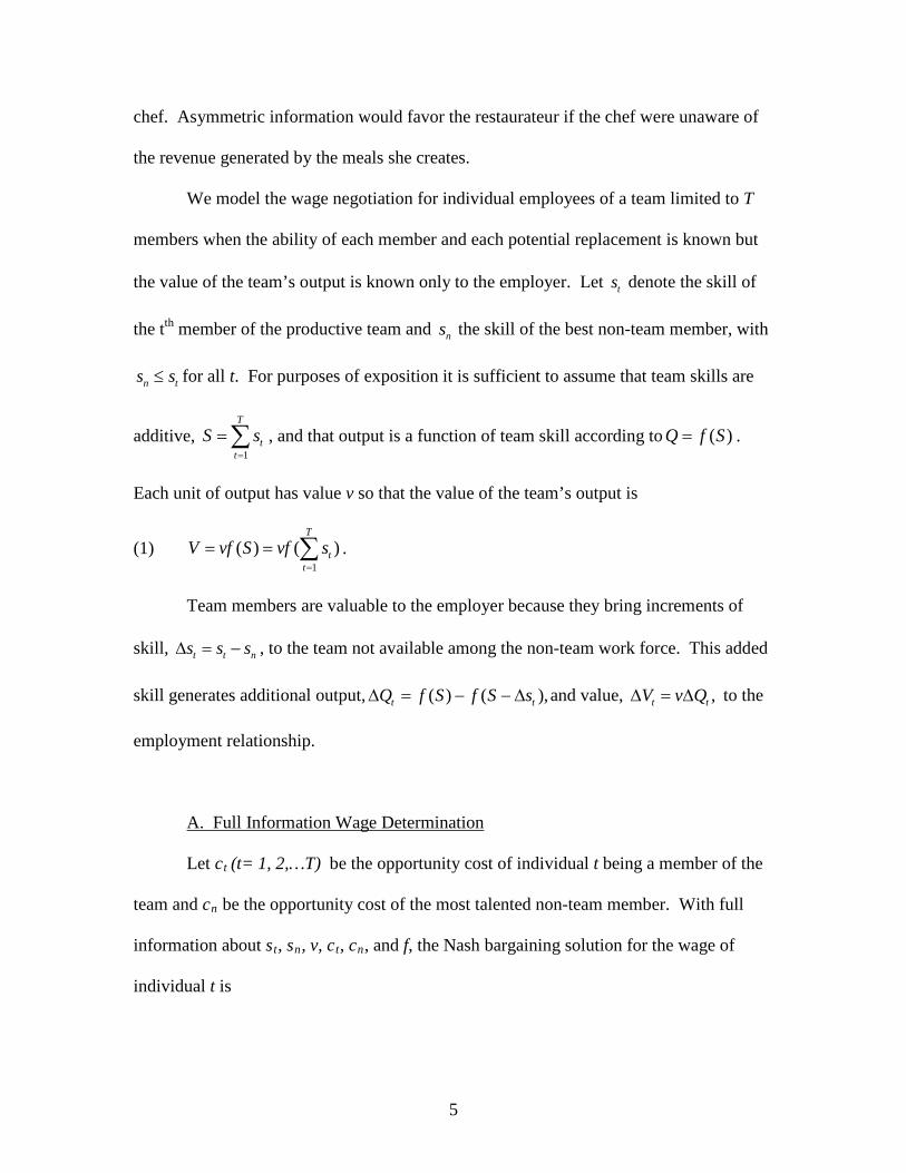
We model the wage negotiation for individual employees of a team limited to T

members when the ability of each member and each potential replacement is known but

the value of the team’s output is known only to the employer. Let ts denote the skill of

the tth member of the productive team and ns the skill of the best non-team member, with

n ts s≤ for all t. For purposes of exposition it is sufficient to assume that team skills are

additive, 1

T

tt

S s=

=∑ , and that output is a function of team skill according to ( )Q f S= .

Each unit of output has value v so that the value of the team’s output is

(1) 1

( ) ( )T

tt

V vf S vf s=

= = ∑ .

Team members are valuable to the employer because they bring increments of

skill, t t ns s s∆ = − , to the team not available among the non-team work force. This added

skill generates additional output, ( ) ( ),t tQ f S f S s∆ = − − ∆ and value, ,t tV v Q∆ = ∆ to the

employment relationship.

A. Full Information Wage Determination

Let ct (t= 1, 2,…T) be the opportunity cost of individual t being a member of the

team and cn be the opportunity cost of the most talented non-team member. With full

information about st, sn, v, ct, cn, and f, the Nash bargaining solution for the wage of

individual t is

6

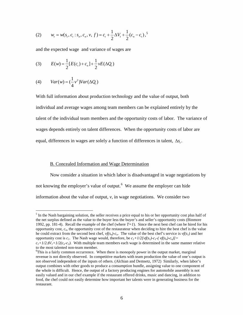
(2) 1 1( , : , , , ) ( )2 2t t t n n t t n tw w s c s c v f c V c c= = + ∆ + − ,5

and the expected wage and variance of wages are

(3) 1 1( ) [ ( ) ] ( )2 2t n tE w E c c vE Q= + + ∆

(4) 21( ) ( ) ( )4 tVar w v Var Q= ∆

With full information about production technology and the value of output, both

individual and average wages among team members can be explained entirely by the

talent of the individual team members and the opportunity costs of labor. The variance of

wages depends entirely on talent differences. When the opportunity costs of labor are

equal, differences in wages are solely a function of differences in talent, .ts∆

B. Concealed Information and Wage Determination

Now consider a situation in which labor is disadvantaged in wage negotiations by

not knowing the employer’s value of output.6 We assume the employer can hide

information about the value of output, v, in wage negotiations. We consider two

5 In the Nash bargaining solution, the seller receives a price equal to his or her opportunity cost plus half of the net surplus defined as the value to the buyer less the buyer’s and seller’s opportunity costs (Binmore 1992, pp. 181-4). Recall the example of the chef (where T=1). Since the next best chef can be hired for his opportunity cost, cn, the opportunity cost of the restaurateur when deciding to hire the best chef is the value he could extract from the second best chef, vf(sn)-cn. The value of the best chef’s service is vf(s1) and her opportunity cost is c1. The Nash wage would, therefore, be c1+1/2[vf(s1)-c1-( vf(sn)-cn)]= c1+1/2∆V1+1/2(cn-c1). With multiple team members each wage is determined in the same manner relative to the most talented non-team member. 6This is a fairly common occurrence. When there is monopoly power in the output market, marginal revenue is not directly observed. In competitive markets with team production the value of one’s output is not observed independent of the inputs of others. (Alchian and Demsetz, 1972) Similarly, when labor’s output combines with other goods to produce a consumption bundle, assigning value to one component of the whole is difficult. Hence, the output of a factory producing engines for automobile assembly is not easily valued and in our chef example if the restaurant offered drinks, music and dancing, in addition to food, the chef could not easily determine how important her talents were in generating business for the restaurant.

7

circumstances of asymmetric information: private negotiations wherein the wage

negotiated by each worker is not known by the other workers, and public negotiations

wherein all workers know the outcome of the other workers’ negotiations. Our intuition

is that in the former situation some workers will be more successful than others in

discovering information about the employer’s value and wages will vary considerably

and in empirically unexplainable ways, while in the latter situation shared knowledge will

help to reduce the variation of wages to that which can be explained by observable

characteristics of labor.

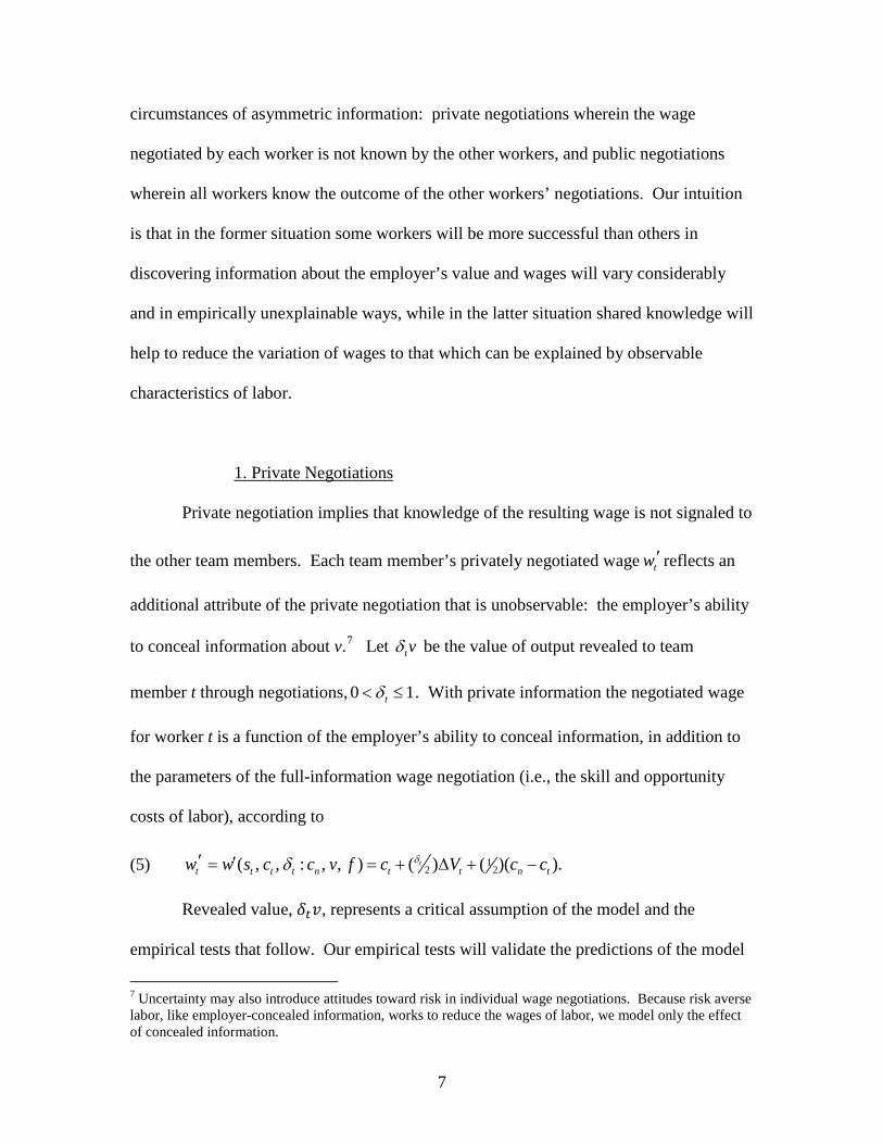
1. Private Negotiations

Private negotiation implies that knowledge of the resulting wage is not signaled to

the other team members. Each team member’s privately negotiated wage tw ′ reflects an

additional attribute of the private negotiation that is unobservable: the employer’s ability

to conceal information about v.7 Let tvδ be the value of output revealed to team

member t through negotiations, 0 1tδ< ≤ . With private information the negotiated wage

for worker t is a function of the employer’s ability to conceal information, in addition to

the parameters of the full-information wage negotiation (i.e., the skill and opportunity

costs of labor), according to

(5) 12 2( , , : , , ) ( ) ( )( ).t

t t t t n t t n tw w s c c v f c V c cδδ′ ′= = + ∆ + −

Revealed value, 𝛿𝑡𝑣, represents a critical assumption of the model and the

empirical tests that follow. Our empirical tests will validate the predictions of the model

7 Uncertainty may also introduce attitudes toward risk in individual wage negotiations. Because risk averse labor, like employer-concealed information, works to reduce the wages of labor, we model only the effect of concealed information.

8

only if tvδ varies significantly from v in the empirical data. There are two sources of

information exchange that might render this difference insignificant. First, if informal

networks sufficed to communicate the information that public negotiations reveal, 𝛿𝑡 = 1

and no new information is revealed by public negotiations. We find evidence of informal

information networks at work in our data when there are private negotiations. Second, to

the extent that public negotiations reveal inaccurate information no convergence is

possible, 𝛿𝑡𝑣 ↛ 𝑣. This might happen for instance if wages were made public but other

dimensions of the employee’s remuneration, such as fringe benefits and work-place

conditions, were not.8

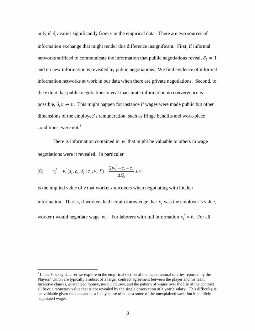
There is information contained in tw ′ that might be valuable to others in wage

negotiations were it revealed. In particular

(6) 2( , , : , , ) t t nt t t t t n

t

w c cv v s c c v f vQ

δ′ − −′ ′= = ≤∆

is the implied value of v that worker t uncovers when negotiating with hidden

information. That is, if workers had certain knowledge that tv ′was the employer’s value,

worker t would negotiate wage .tw ′ For laborers with full information .tv v′ = For all

8 In the Hockey data set we explore in the empirical section of the paper, annual salaries reported by the Players’ Union are typically a subset of a larger contract agreement between the player and his team. Incentive clauses, guaranteed money, no-cut clauses, and the pattern of wages over the life of the contract all have a monetary value that is not revealed by the single observation of a year’s salary. This difficulty is unavoidable given the data and is a likely cause of at least some of the unexplained variation in publicly negotiated wages.

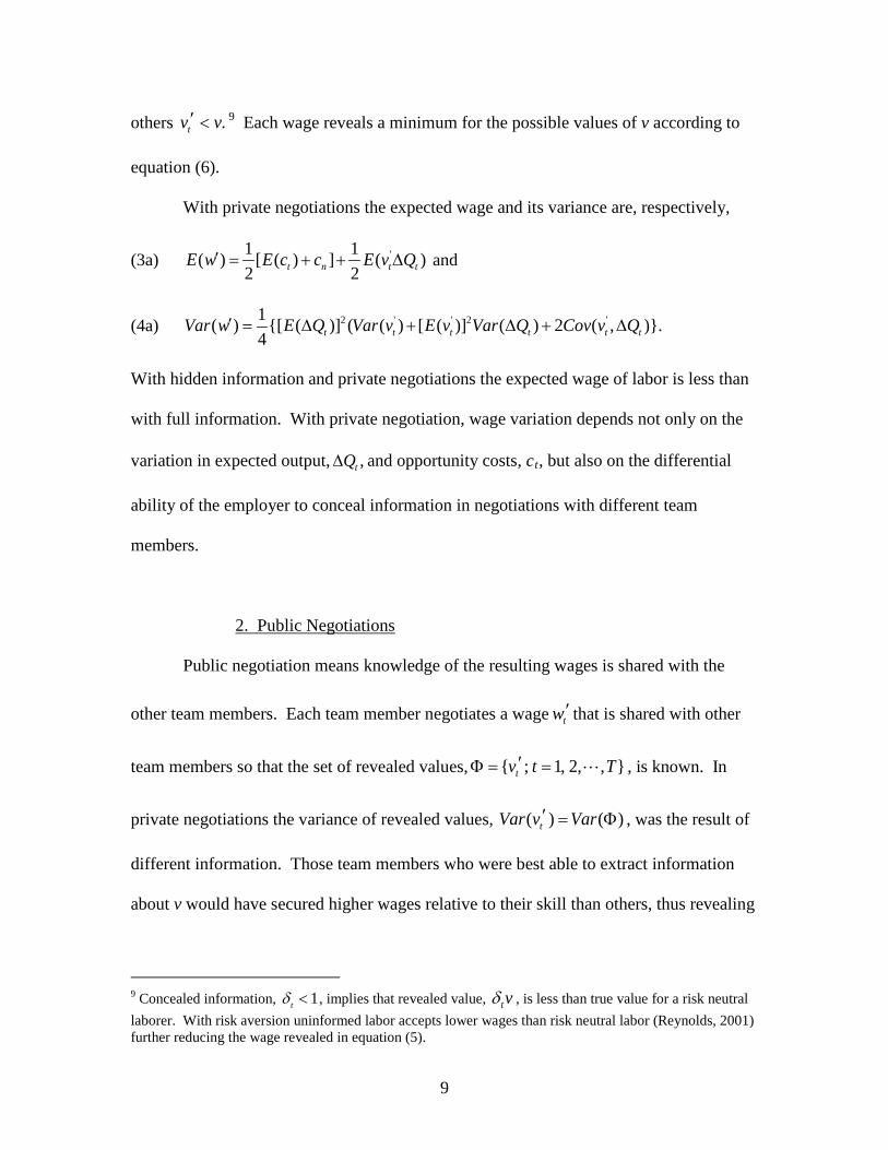
9

others .tv v′ < 9 Each wage reveals a minimum for the possible values of v according to

equation (6).

With private negotiations the expected wage and its variance are, respectively,

(3a) '1 1( ) [ ( ) ] ( )2 2t n t tE w E c c E v Q′ = + + ∆ and

(4a) 2 ' ' 2 '1( ) {[ ( )] ( ( ) [ ( )] ( ) 2 ( , )}.4 t t t t t tVar w E Q Var v E v Var Q Cov v Q′ = ∆ + ∆ + ∆

With hidden information and private negotiations the expected wage of labor is less than

with full information. With private negotiation, wage variation depends not only on the

variation in expected output, ,tQ∆ and opportunity costs, ct, but also on the differential

ability of the employer to conceal information in negotiations with different team

members.

2. Public Negotiations

Public negotiation means knowledge of the resulting wages is shared with the

other team members. Each team member negotiates a wage tw ′ that is shared with other

team members so that the set of revealed values, { ; 1, 2, , }tv t T′Φ = = , is known. In

private negotiations the variance of revealed values, ( ) ( )tVar v Var′ = Φ , was the result of

different information. Those team members who were best able to extract information

about v would have secured higher wages relative to their skill than others, thus revealing

9 Concealed information, 1tδ < , implies that revealed value, tvδ , is less than true value for a risk neutral laborer. With risk aversion uninformed labor accepts lower wages than risk neutral labor (Reynolds, 2001) further reducing the wage revealed in equation (5).

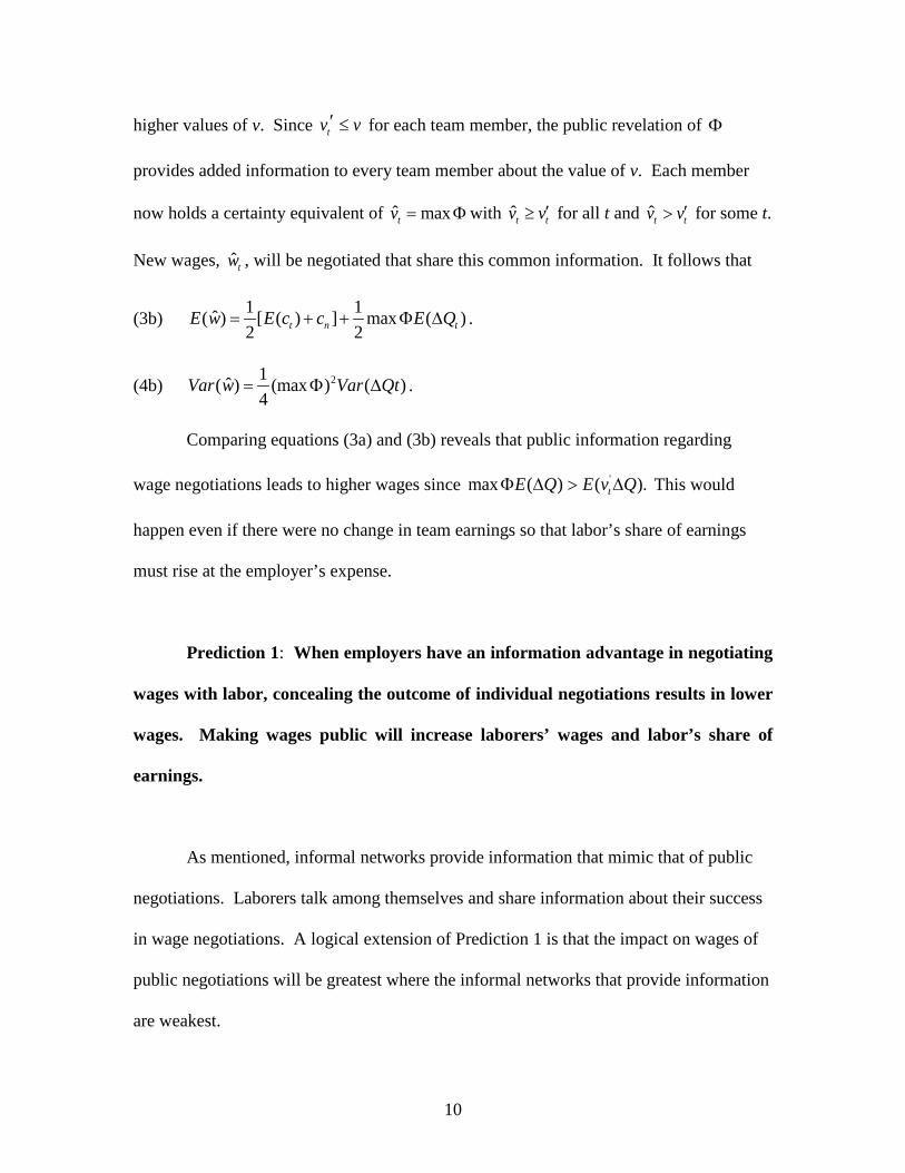
10

higher values of v. Since tv v′ ≤ for each team member, the public revelation of Φ

provides added information to every team member about the value of v. Each member

now holds a certainty equivalent of ˆ maxtv = Φwith t̂ tv v′≥ for all t and t̂ tv v′> for some t.

New wages, ˆ tw , will be negotiated that share this common information. It follows that

(3b) 1 1ˆ( ) [ ( ) ] max ( )2 2t n tE w E c c E Q= + + Φ ∆ .

(4b) 21ˆ( ) (max ) ( )4

Var w Var Qt= Φ ∆ .

Comparing equations (3a) and (3b) reveals that public information regarding

wage negotiations leads to higher wages since 'max ( ) ( ).tE Q E v QΦ ∆ > ∆ This would

happen even if there were no change in team earnings so that labor’s share of earnings

must rise at the employer’s expense.

Prediction 1: When employers have an information advantage in negotiating

wages with labor, concealing the outcome of individual negotiations results in lower

wages. Making wages public will increase laborers’ wages and labor’s share of

earnings.

As mentioned, informal networks provide information that mimic that of public

negotiations. Laborers talk among themselves and share information about their success

in wage negotiations. A logical extension of Prediction 1 is that the impact on wages of

public negotiations will be greatest where the informal networks that provide information

are weakest.

11

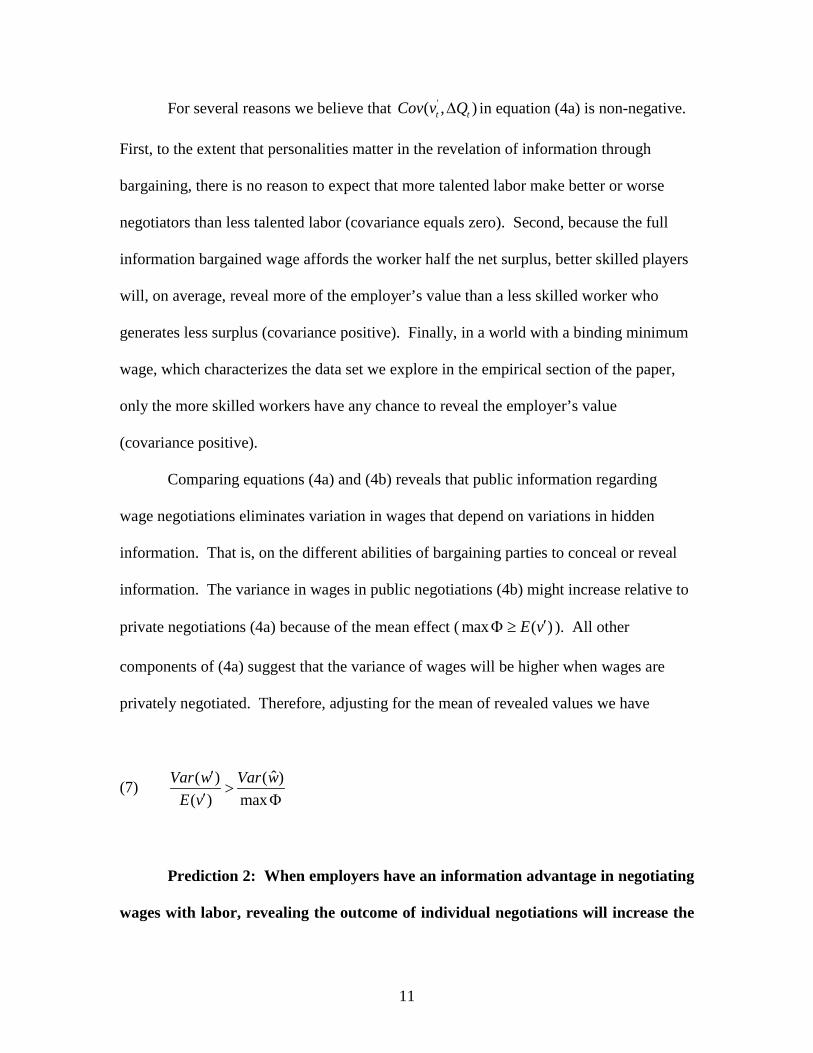
For several reasons we believe that '( , )t tCov v Q∆ in equation (4a) is non-negative.

First, to the extent that personalities matter in the revelation of information through

bargaining, there is no reason to expect that more talented labor make better or worse

negotiators than less talented labor (covariance equals zero). Second, because the full

information bargained wage affords the worker half the net surplus, better skilled players

will, on average, reveal more of the employer’s value than a less skilled worker who

generates less surplus (covariance positive). Finally, in a world with a binding minimum

wage, which characterizes the data set we explore in the empirical section of the paper,

only the more skilled workers have any chance to reveal the employer’s value

(covariance positive).

Comparing equations (4a) and (4b) reveals that public information regarding

wage negotiations eliminates variation in wages that depend on variations in hidden

information. That is, on the different abilities of bargaining parties to conceal or reveal

information. The variance in wages in public negotiations (4b) might increase relative to

private negotiations (4a) because of the mean effect ( max ( )E v′Φ ≥ ). All other

components of (4a) suggest that the variance of wages will be higher when wages are

privately negotiated. Therefore, adjusting for the mean of revealed values we have

(7) ˆ( ) ( )

( ) maxVar w Var w

E v′>

′ Φ

Prediction 2: When employers have an information advantage in negotiating

wages with labor, revealing the outcome of individual negotiations will increase the

12

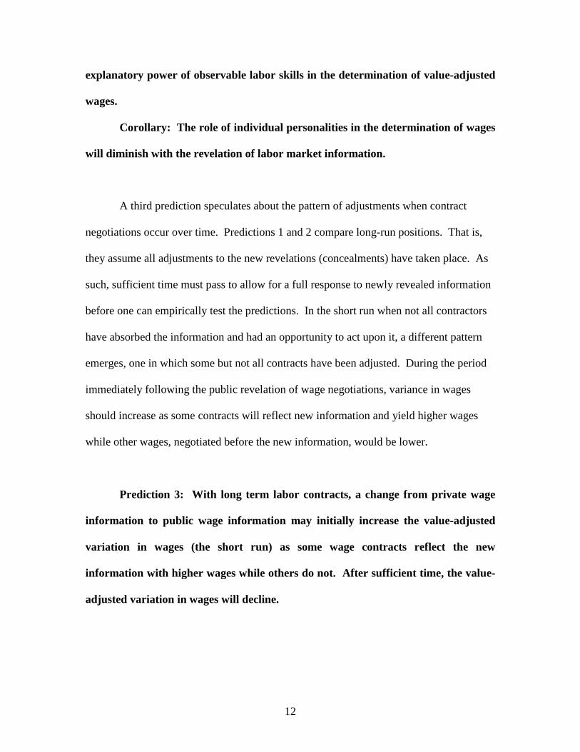
explanatory power of observable labor skills in the determination of value-adjusted

wages.

Corollary: The role of individual personalities in the determination of wages

will diminish with the revelation of labor market information.

A third prediction speculates about the pattern of adjustments when contract

negotiations occur over time. Predictions 1 and 2 compare long-run positions. That is,

they assume all adjustments to the new revelations (concealments) have taken place. As

such, sufficient time must pass to allow for a full response to newly revealed information

before one can empirically test the predictions. In the short run when not all contractors

have absorbed the information and had an opportunity to act upon it, a different pattern

emerges, one in which some but not all contracts have been adjusted. During the period

immediately following the public revelation of wage negotiations, variance in wages

should increase as some contracts will reflect new information and yield higher wages

while other wages, negotiated before the new information, would be lower.

Prediction 3: With long term labor contracts, a change from private wage

information to public wage information may initially increase the value-adjusted

variation in wages (the short run) as some wage contracts reflect the new

information with higher wages while others do not. After sufficient time, the value-

adjusted variation in wages will decline.

13

III. Testing the Model’s Predictions

We test the predictions of the model using data from player salaries in the

National Hockey League. In 1989 the National Hockey League Players’ Association first

published the salaries of every player in the League. Prior to this, players knew only their

own salary with precision.10 Players would have been underpaid in the sense that they

captured less than half the surplus they generated and some players would have been

greatly underpaid. When it is revealed that another player with similar performance

statistics has a higher salary, an owner that had successfully hidden revenue information

in bargaining would no longer be able to do so to the same degree.11 In addition, an

owner’s claim that he or she can hire an alternate player at a favorable salary is reduced

and the player’s sense of his opportunity cost of playing for another team rises.12

To test Prediction 1 we collected annual salary data

from www.hockeyzoneplus.com. Canadian salaries were converted to US dollars by the

site. Team revenue data were collected annually; first from Financial World magazine

and later from Forbes magazine. Financial World began compiling estimates of

10 In the early 1970s several authors estimated salary equations for players in Major League Baseball using data reported in the popular press before the player’s union first revealed salaries [see for example, Pascal and Rapping (1972) and Scully (1974a, 1974b)]. The quality of the regressions in terms of the ability to explain variations in salary were quite good. In part, this is explained by the fact that the samples were heavily weighted with high salaried players who stand out in performance as well as in salaries. However, some, unknown, amount of the variation might be explained by informal networks that disseminate information to be used like the formal information we model in this paper. To the extent that this happens, the results we search for in this paper will be more difficult to find. 11 Knowledge of the model of salary negotiation forecloses the reciprocal argument that owners who had previously paid more could use the new knowledge to bargain for reductions in wages for their players. Knowing that information is asymmetric suggests to the players that errors are systematically biased in favor of owners. 12 There were between 20 and 24 teams and owners over the study period. Arbitrage equates the marginal value of talent across teams making salary comparisons across teams valid. (Rottenberg, 1956; Scully, 1974a).

14

revenues for teams in the four major North American sports leagues in the 1980s. When

Financial World ceased publication, Forbes continued the series.

Team salary relative to team revenue can change because of factors other than the

new information - e.g., League expansion, the liberalization of free agency rules, changes

in the collective bargaining agreement or the hubris of owners. Fortunately for our

purposes, the impact of new information will occur only once following the revelation of

salaries - salaries relative to team value will rise significantly during the subsequent

period when contracts are renegotiated with new information and then return to a normal

pattern of increase or decrease. A period of five years from 1989 to 1994 is chosen to

permit all contracts to be renegotiated. The period 1994 to 2004 serves as a baseline to

test the implications of Prediction 1.

Table 1 presents summary statistics of NHL player salaries relative to team

revenues for skaters and goalies. Individual salaries are normalized by league revenue

per roster spot. This permits an analysis of variance to test whether player shares (and,

by extension, the rate of increase in player shares) were greater in the period immediately

following the revelation of all player salaries than in other periods. In 1989 goalies and

skaters were similarly paid, collecting about 22% of the available revenue. By 1994

skater salaries had risen to 36% and goalies to 45% of available revenue. This represents

a 64% growth in skaters’ share and a whopping 103% increase in goalies’ share. In the

next decade skaters’ share grew 27% each five year period and goalies share grew 25%

per five year period.

[Table 1 here]

15

As indicated, player shares continued to grow from 1989 to 2004. The authors

suspect that this trend began with the formation of the NFLPA in 1967 and was fueled by

free agency and a lack of fiscal control or simple hubris among team owners. As this

trend could not continue indefinitely, owners locked players out of the 2004-05 season

and a hard salary cap set as a fraction of revenues was negotiated. Hence, 2004 was the

last year salaries relative to revenue could rise. We test the null hypothesis that player

shares did not increase more than usual during the period 1989 to 1994 and reject this for

both skaters and goalies at the 98% and 99% confidence levels, respectively. That is, the

14 and 23 percentage point increase in player shares for skaters and goalies, respectively,

during the first five years were significantly greater than the 11 and 13 percentage point

five-year average increases witnessed during the 1994-2004 period. As the absolute five-

year increase is greater during 1989-1994 the growth rate, calculated from a smaller base,

must also be significantly greater, confirming Prediction 1.

We speculated that informal information networks might offset some of the

information disadvantage as players share information purposefully or inadvertently

about the success of their private negotiations. These networks would function best

among players on the same team as communication and trust is greatest here and

observations of life style can provide tangential information. Teams typically carry only

two goalies, the starter and a backup, and 21 skaters.13 As goalies and skaters have

different skill sets and perform different tasks, a starting goalie would have only his back-

up for comparison in this informal network. Among skaters there are five starters (first

line players); the rest being second, third, and fourth line players. We posit that the

13 While there is no limit on the number of goalies allowed on the 23 man roster, most teams carry only two. Only 2 goalies and 18 skaters are allowed to dress for each game.

16

amount of informal information on skaters’ salaries relative to goalies’ salaries in 1989 is

greater and that goalies will benefit more from public information when it is revealed. A

test of the null hypothesis that goalies’ salaries relative to revenue did not increase more

than skaters’ relative salaries yields a t-value of 1.9442 and is rejected with more than

95% confidence.

Predictions 2 and 3 involve the explanatory power of observed characteristics of

labor and personality in salary determination. Because talent in hockey has many

dimensions we use regression analysis to account for the mean effects of talent attributes

and rely on the coefficient t-statistics and regression R2 statistic to reveal the magnitude

and power of these variables to explain salaries across time. If Prediction 2 is correct,

performance statistics will gain importance as indicated by higher and more significant t-

statistics in determining salaries and the personalities of the salary negotiators will cease

to matter once salary information is made public. If prediction 3 is correct, the R2

statistic from annual regressions will first decline and then increase.14

Following the sports literature for hockey we identify performance statistics that

indicate the observed skills of each player and are used in the regression analysis. Data

were collected from several sources. Performance statistics were obtained online from

the site www.hockeydb.com. Allstar appearances are given in the NHL page on

Wikipedia. Salary data were obtained from www.hockeyzoneplus.com. Canadian

salaries were converted to US dollars by the site. Team revenue data were collected

annually from Financial World magazine.

14 The impact of opportunity cost in determining wages in equation (5) is not relevant to the present analysis. The NHL has a minimum salary structure that almost certainly exceeds the opportunity cost of all players and dictates the price an owner must pay for replacement talent. Since each player could sign for the minimum wage without bargaining, the minimum salary defines a player’s opportunity cost as well as the cost of replacement players (ct = cn).

17

1989/90 is the obvious starting point for the study as it is the first year salary data

are provided and therefore represents the last year when all players’ contracts were

negotiated with information asymmetries. 1993/94 was chosen as the last year because

the subsequent strike truncated the reported salary data and altered the collective

bargaining rules. Nearly all contracts will have been re-negotiated within five years.

Two data sets, one of skater and one of goalies, were assembled because goalies have

different performance characteristics than do skaters. We collected performance data for

all players under contract in these years that had at least some NHL experience in two

prior seasons. There are two reasons for requiring two years of prior experience. First,

we posit that performance expectations are created by past performance and use lagged

performance measures as explanatory variables. Hence, some prior NHL performance is

needed to measure expected performance during the contract period. In addition, there

was a significant influx of highly-skilled players from the former Soviet Union and its

satellites starting in 1992. These players were often paid well but had no prior NHL

performance statistics. Limiting our study to players with at least two years of

experience eliminates them. There were between 34 and 44 observations of goalies over

time and between 324 and 389 observations of skaters over the study period.15

With full information, arbitrage among owners equates the marginal value of

talent in producing revenue across teams so that team identity is not typically included as

an explanatory variable in sports salary regressions.16 However, with concealed

information owners (or players) who are better salary negotiators will reveal lower

(higher) values than owners (or players) who are less adept at negotiation. We presented

15 The NHL expanded the number of teams and players under contract, adding one team in 1991, two teams in 1992 and two more in 1993. 16 Rottenberg (1956).

18

this as a Corollary to Prediction 2. To test this we include team dummy variables to

proxy for owner talent in bargaining with the expectation that the relevance of owner

bargaining skills will decline as time passes and information is revealed.17 Because of

the scarce number of goalies, team dummies could only be estimated in the skaters’ data

set.

Definitions of the variables employed are presented below. Table 2 presents

summary statistics for salaries in the various data sets.

A. Salary variables:

SALARY: Nominal salary in US Dollars

ADJSAL: Nominal salary divided by revenue per rostered player.

B. Performance statistics used in the salary regressions for goalies and skaters include:

EXP: The number of years the player has been in the NHL prior to the current

season.

GAMES: The number of games played in the previous season..

ALLSTAR: The number of times a player was named either first or second team

all NHL prior to the current season.

C. Performance statistics used in the salary regressions for goalies only include:

GAA: The goals against average in the previous season.

SHOTS: The number of shots faced in the previous season.

D. Performance statistics used in the salary regressions for skaters only include:

GOALSSQUARED: The number of goals in the previous season squared

ASSISTS: The number of assists in the previous season.

17 It would be interesting to test whether player personalities mattered. However, there are very few identical salaries, except those players earning the minimum wage, so that a matrix of dummies for individual players is nearly perfectly correlated with player salaries making such a test impossible.

19

PENMIN: The number of penalty minutes in the previous season.

DEF: A dichotomous variable that takes the value 1 if the player is a defenseman

and 0 otherwise.

E. Team dummy variables. The Washington Capitals was chosen as the control team for

the following reasons. First, it was a good team – it made the playoffs each year – but

not a great team – it never reached the Stanley Cup Finals, and only once made the

conference championship. Second, it had the same owner throughout the study. Finally it

is in the US, so any issues with exchange rates are minimized.

F. Revenue. Team by team revenue from Financial World.

G. CAN A dummy variable for players on Canadian teams was employed in the goalies

regression to control for exchange rate fluctuations between the contracting period and

the year of observation.

H. EXPAND During the time of this study the NHL expanded three times, adding one

team in 1991 and two teams in both 1992 and 1993. Any potential differences in

expansion teams were captured by a dummy variable for players on expansion teams.

[Table 2 Here]

To test Predictions 2 and 3 concerning the explanatory power of performance

statistics and personalities we estimate the parameters in a set of salary regressions of the

general form

Yi = a0 + ajXij+ bkZik + ei,

where Yi is player i’s salary, Xij is a matrix of performance statistics assigning the

previous season’s performance characteristic j to player i, and Zik is a matrix of non-

20

performance explanatory variables assigned to player i. The a’s and b’s are estimated

parameters and e is the error term.

For goalies there is strong correlation between save percentage (the other most

commonly-employed performance statistic) and goals-against-average, so only goals

against average was used in the analysis that follows. The number of shots the goalies

faced was calculated from the statistics and included in the regressions. For skaters the

number of goals squared rather than the number of goals was included for two reasons.

First, goals and assists are highly correlated, enough so as to raise concerns of

multicolinearity. Second, the perceived value to a team of a goal scorer is convex in

goals (a player with 50 goals is more than twice as valuable as one with 25). Estimates of

regression coefficients were obtained via OLS. As there is a problem with

heteroskedasticity the standard errors relied on for inference are the robust errors

calculated in the method put forth by White (1980).

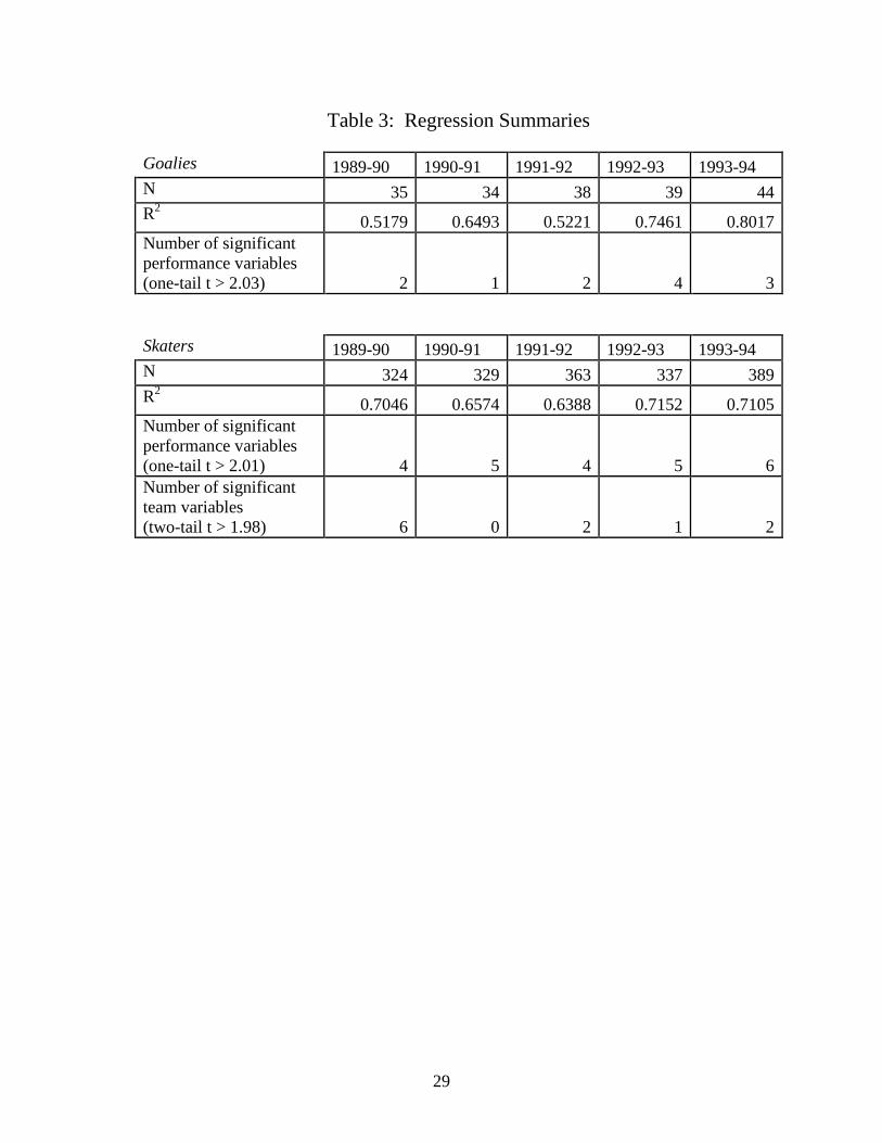
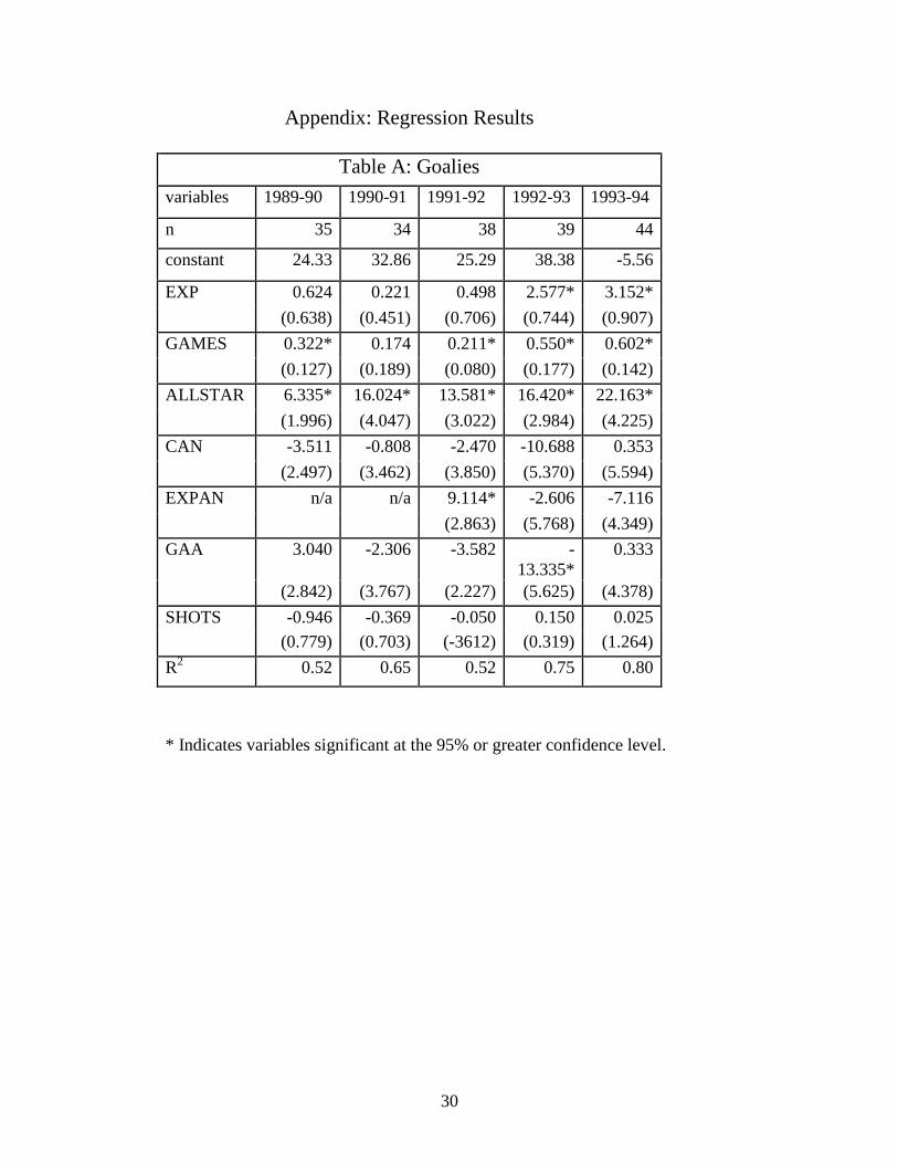
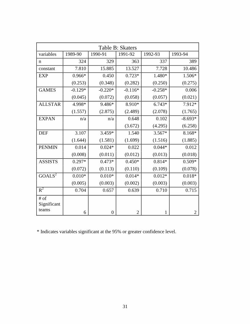
Table 3 presents the relevant regression results for the two data sets.18 To test

Prediction 3 we compare the R2 statistic from consecutive years. Prediction 3 is that R2

should decrease in the second, and perhaps, third year when not all contracts have been

renegotiated and increase thereafter. The skaters’ data set follows this pattern precisely.

In 1989 team and performance variables explained 70% of the salary variation. By 1991

the explanatory power of these variables had decreased to 64% but increased to 71% in

1992 and 1993. In the goalies’ data set the explanatory power of the model is constant in

the first and third year (52%) with an anomalous increase in the second year. The fourth

and fifth years demonstrate a steady increase in the explanatory power of the

performance variables increasing to 80% by the end of the study period. 18 Coefficient estimates and their standard errors are presented in the Appendix.

21

[Table 3 Here]

As further evidence we ask how many of the performance variables are significant

at the 95% confidence level. For the performance statistics this is a one-tailed test. In the

Goalies’ data set there are five such variables: EXP, GAMES, ALLSTAR, GAA and

SHOTS. Of these SHOTS is perhaps the weakest predictors of salary as SHOTS reflects

not only the pressure a goalie faced but also the quality of the defense that supports him.

It is not surprising that it is never significant. The variable ALLSTAR is significant in all

years. In the first two years the variable GAMES was the only other significant variable

and is significant in 4 of the 5 years. Unlike skaters, goalies are rarely substituted and

usually play the entire game. As such, the front-line goalie plays a significantly larger

number of games than the back up and GAMES is positively and significantly associated

with SALARY in each season except 1990-91. By the end of the study period two other

variables – EXP and GAA - had become significant.

In the skaters’ data set there are seven performance variables: GAMES,

PENMIN, ASSISTS, EXP, ALLSTAR, GOALSQUARED and DEF. Unlike with goal

tenders, the variable GAMES has a negative and significant sign in four of the five years.

Skaters are substituted regularly, often in groups known as lines. The first and second

line skaters are the better (higher paid) players and play significantly more minutes per

game than players on the third and fourth line. They are rested and held out of games for

injuries more frequently than third and fourth line players, who play fewer minutes but

more games. Data on minutes played, a better measure of a player’s contribution, were

22

not available. In Table 3 the significance of GAMES is ignored. In 1989 four of the

remaining six explanatory variables were significant. By 1994 all six were significant.19

Predictions 2 and 3 are thus confirmed for both data sets. The explanatory power

as well as the number and importance of the explanatory variables rises significantly after

the revelation of information. Mixing new contracts formed after the revelation of

information with those formed before increases the unexplained variation during the

interim years of the study.

Finally we turn our attention to the impact of owner and front office personalities

in the determination of salaries. For this test we can only use the skaters’ data set.

Including dummy variables for teams is not possible in the goalie data set as there are at

most two goalies per team. Based on the 95% level of confidence used to reject the null

hypothesis that the personalities of team negotiators were NOT important, the probability

of wrongly identifying the TEAM variable as significant when it is not is only five-

percent (5%). Thus with 26 teams in 1993 the likelihood of the null hypothesis being

rejected for one is quite high. The expected number of Type I errors in 1993 is 1.3.

However, the six teams identified as having a significant impact on salary negotiations in

1989 when there were only 21 teams could not possibly be the result of a Type I error.

The expected number of Type I errors in 1989 is 1.05 with a standard deviation of .9988.

We conclude that personalities that were so important in salary negotiations before the

revelation of information lost all significance after and confirm the Corollary to

Prediction 2.

IV. Conclusions 19 Including GAMES does not change this relationship as GAMES was significant in both of these years.

23

Wage bargaining favors the individual with superior information. In particular,

managers with superior knowledge of labor’s marginal revenue product can suppress

wages and separate, to some degree, earnings from performance. In this setting, wages

tend toward the lower bound of possible wages. This increases the share of revenue

captured by management. When information asymmetries are removed, wages and

labor’s share of income rises and wages are better explained by the performance of labor.

Personalities that were so important in determining the bargaining outcome when

information was private become immaterial to the determination of wages when

information is public.

In the National Hockey League public reporting of every NHL player’s salary

began in 1989. At the time, average salary was just over $200,000 US and player

performance did not reasonably explain variations in salary among players. Within five

years average player salary had more than tripled. During this period players’ share of

revenue increased 64% for skaters and 103% for goalies. This rapid increase far exceeds

the increase in any other period for which data are available and is the direct cause of the

owners’ lockout in 2004 and the subsequent cap on player salaries as a fixed percent of

team revenues that was collectively bargained to end the lockout.

Prior to the revelation of salary information, the personalities of team owners and

the front office personnel that negotiate with players over their individual wage were

highly significant and the performance statistic of players compared to others in the

league much less so. After wages became public information personalities lost all

significance and a player’s performance relative to others in the league became the

predominant determinant of salary. This effect was most profound for goalies who, prior

24

to the revelation of all players’ salaries, would have had little opportunity for informal

comparisons with other goalies with similar performance statistics. It would be

interesting to test whether a player’s agent had an effect on his salary prior to 1989. Our

model would predict that an agent with more players and with players on more teams,

would have an advantage over another agent in salary negotiations. Unfortunately, to our

knowledge, this information is not readily available.

Finally, the short run adjustment to new information caused an increase in

unexplained variation among salaries as some salaries were being renegotiated while

others had not. We tried without success to identify the timing of each player’s contract

negotiations. Short-run increases in salary variation could then be explained. This

remains an area for further investigation.

25

References

Akerlof, George A. (1970), “The Market for ‘Lemons:’ Quality Uncertainty and the

Market Mechanism,” Quarterly Journal of Economics, 84, 488-500.

Alchian, Allen and Harold Demsetz (1972), “Production, Information Costs, and

Economic Organization,” American Economic Review, 62, 777-795.

Ausubel, Lawrence M., Peter Crampton, and Raymond J. Deneckere, “Bargaining with

Incomplete Information,” Handbook of Game Theory, Vol. 3, Chapter 50, Robert J.

Aumann and Sergiu Hart, editors, Elsevier Science, Amsterdam, 2002.

Binmore, Ken (1992), Fun and Games: A Text on Game Theory, Lexington: D.C. Heath

Crampton, Peter and Joseph Tracy (1992), “Strikes and Holdouts in Wage Bargaining:

Theory and Data,” American Economic Review, 82, 100-21.

Grossman, Sanford J. (1981), “The Informational role of Warranties and Private

Disclosure About Product Quality,” Journal of Law and Economics, 24, 461-83.

Nelson, Phillip (1974), “Advertising as Information,” Journal of Political Economy, 84,

729-54.

26

Pascal, A. H. and Rapping, L. A. (1972) The Economics of Racial Discrimination in

Organized Baseball, in Racial Discrimination in Economic Life (Ed.) A. H. Pascal, D. C.

Heath, Lexington, Massachusetts, pp. 119-56.

Reynolds, Stanley S. (2001), “Multi-period Bargaining: Asymmetric Information and

Risk Aversion,” Economic Letters, 72, 309-15.

Rottenberg, Simon. (1956), “The Baseball Players’ Market.” Journal of Political

Economy, 64, 242–58.

Scully, Gerald W. (1974a), “Pay and Performance in Major League Baseball,” American

Economic Review, 64, 915-930.

Scully, G. W. (1974b) Discrimination: The Case of Baseball, in Government and the

Sports Business(Ed.) R.G. Noll, Brookings Institution, Washington, DC, pp. 221-73.

Spence, A. Michael (1974), Market Signaling: Informational Transfer in Hiring and

Related Screening Processes, Cambridge: Harvard University Press.

White, Halbert (1980), “A Heteroskedasticity-Consistent Covariance Matrix Estimator

and Direct Test for Heteroskedasticity,” Econometrica, 48, 817-838.

27

Table 1: Summary of Players' Salaries Relative to Team Revenue per Position

Year 1989 1994 2004 Skaters Mean 0.2215 0.3629 0.5858 Standard Deviation 0.1571 0.3159 0.6024 Number 499 559 615 Five Year Growth Rate 0.6384 0.2705 Five Year Change 0.1414 0.1115

H0: 0.1414 ≤ 0.1115 t = 1.9841

Goalies Year 1989 1994 2004 Mean 0.2220 0.4513 0.7075 Standard Deviation 0.1072 0.3284 0.5775 Number 53 59 63 Five Year Growth Rate 1.0331 0.2521 Five Year Change 0.2293 0.1281

H0: 0.2293 ≤ 0.1281 t = 2.2384 H0: 0.2293 ≤ 0.1414 t = 1.9442

28

Table 2: Summary Statistics Goalies 1989-90 1990-91 1991-92 1992-93 1993-94 N 35 34 38 39 44

Mean salary 224,237 287,061 292,333 458,573 672,272 Mean adjusted Salary in % 24.63 26.78 25.74 36.49 49.21 Standard deviation of

adjusted salary 10.096 15.972 16.688 27.645 35.274

Skaters 1989-90 1990-91 1991-92 1992-93 1993-94

N 324 329 363 337 389

Mean salary 228,463 276,676 341,331 405,736 572,303 Mean adjusted Salary in % 25.10 25.81 30.59 32.28 41.89 Standard deviation of

e adjusted salary 17.874 23.277 25.537 27.685 32.828

29

Table 3: Regression Summaries Goalies 1989-90 1990-91 1991-92 1992-93 1993-94 N 35 34 38 39 44 R2 0.5179 0.6493 0.5221 0.7461 0.8017 Number of significant performance variables (one-tail t > 2.03) 2 1 2 4 3

Skaters 1989-90 1990-91 1991-92 1992-93 1993-94 N 324 329 363 337 389 R2 0.7046 0.6574 0.6388 0.7152 0.7105 Number of significant performance variables (one-tail t > 2.01) 4 5 4 5 6 Number of significant team variables (two-tail t > 1.98) 6 0 2 1 2

30

Appendix: Regression Results

Table A: Goalies

variables 1989-90 1990-91 1991-92 1992-93 1993-94

n 35 34 38 39 44

constant 24.33 32.86 25.29 38.38 -5.56

EXP 0.624 0.221 0.498 2.577* 3.152* (0.638) (0.451) (0.706) (0.744) (0.907)

GAMES 0.322* 0.174 0.211* 0.550* 0.602* (0.127) (0.189) (0.080) (0.177) (0.142)

ALLSTAR 6.335* 16.024* 13.581* 16.420* 22.163* (1.996) (4.047) (3.022) (2.984) (4.225)

CAN -3.511 -0.808 -2.470 -10.688 0.353 (2.497) (3.462) (3.850) (5.370) (5.594)

EXPAN n/a n/a 9.114* -2.606 -7.116 (2.863) (5.768) (4.349)

GAA 3.040 -2.306 -3.582 -13.335*

0.333

(2.842) (3.767) (2.227) (5.625) (4.378) SHOTS -0.946 -0.369 -0.050 0.150 0.025

(0.779) (0.703) (-3612) (0.319) (1.264) R2 0.52 0.65 0.52 0.75 0.80

* Indicates variables significant at the 95% or greater confidence level.

31

Table B: Skaters variables 1989-90 1990-91 1991-92 1992-93 1993-94 n 324 329 363 337 389 constant 7.810 15.885 13.527 7.728 10.486 EXP 0.966* 0.450 0.723* 1.480* 1.506*

(0.253) (0.348) (0.282) (0.250) (0.275) GAMES -0.129* -0.220* -0.116* -0.258* 0.006

(0.045) (0.072) (0.058) (0.057) (0.021) ALLSTAR 4.998* 9.486* 8.910* 6.743* 7.912*

(1.557) (2.875) (2.489) (2.078) (1.765) EXPAN n/a n/a 0.648 0.102 -8.693*

(3.672) (4.295) (6.258) DEF 3.107 3.459* 1.540 3.567* 8.168*

(1.644) (1.581) (1.699) (1.516) (1.885) PENMIN 0.014 0.024* 0.022 0.044* 0.012

(0.008) (0.011) (0.012) (0.013) (0.018) ASSISTS 0.297* 0.473* 0.450* 0.814* 0.509*

(0.072) (0.113) (0.110) (0.109) (0.078) GOALS2 0.010* 0.010* 0.014* 0.012* 0.018*

(0.005) (0.003) (0.002) (0.003) (0.003) R2 0.704 0.657 0.639 0.710 0.715

# of Significant teams 6 0 2 1 2

* Indicates variables significant at the 95% or greater confidence level.