ASYMMETRIC INFORMATION, BARGAINING

AND UNEMPLOYMENT FLUCTUATIONS*

Daron Acemoglu1

Department of EconomicsMassachusetts Institute of Technology

JEL Classification: E32Keywords: Asymmetric Information, Bargaining, Dynamic Wage Sluggishness,

Unemployment, Persistence.

AbstractWe construct a dynamic general equilibrium model where wages are determined by bilateral

bargaining and the firm has superior information. The asymmetry of information introducesunemployment fluctuations and dynamic wage sluggishness. Because the information of the firm is onlyrevealed gradually, wages fall slowly in response to a negative shock and unemployment exhibitsadditional persistence. It is shown that high job destruction will generally be followed by a period ofhigher than average job destruction, that the presence of common shocks introduces an informationalexternality, and that bargaining is an inefficient method of wage determination as compared to implicitcontracts.

* Submitted April 1993, Final Version accepted February 1995.

1

1. Introduction

Unemployment both in the US and Europe exhibits considerable persistence; a period of high

unemployment is usually followed by further periods of higher than average unemployment (see for

instance Jaeger and Parkinson 1994). Existing theories have difficulty in explaining this high level of

persistence. In this paper we argue that dynamic bargains and asymmetric information in the wage

determination process can be an additional source of persistence in unemployment fluctuations.

The main intuition is simple; in non-competitive labor markets, both workers and firms receive

rents from the employment relation. However, if one of the parties is imperfectly informed about the size

of the total rents to be distributed, their demand can be excessively high leading to a premature

termination of the employment relation. This feature in our model will lead to the destruction of jobs.

However, in a dynamic bargaining framework, agreements often take time and the relevant information

is only revealed gradually. Thus when a bad shock hits the economy, the severity of this shock is only

revealed slowly and this creates what we call "dynamic wage sluggishness". Wages are not only high

(relative to the marginal product of labor) now but also in the future periods because, with dynamic

bargaining, not all the relevant information about the severity of the shock is revealed immediately.

Therefore a temporary shock will not only lead to jobs being destroyed in the current period but also in

the periods to come. In other words, when information relevant to the formation of wages is only spread

slowly, the adverse effects of this shock will also be spread out over time.

To capture these features we will consider a dynamic general equilibrium model in which the

marginal product of labor is only observed by firms. Jobs are created when unemployed workers are

matched with new firms. Yet the job can be destroyed if the worker and the firm fail to agree on the wage

rate. We will analyze the behavior of this economy in the presence of aggregate and idiosyncratic shocks

to the marginal product of labor and show that the presence of private information will lead to

amplification of the impact of shocks on employment fluctuations and to additional persistence.

2

This channel of persistence differs from the existing ones in the literature; the most usual channel

of persistence in the literature relies on sluggish job creation. A shock increases the unemployment level

and the unemployed workers cannot easily get back into jobs. This can be because of search (e.g.

Pissarides (1985), Wright (1986)) or due to insiders who ask for higher wages and prevent an expansion

of employment (e.g. Lindbeck and Snower (1988), Blanchard and Summers (1986)) or because

unemployed workers lose their skills (Pissarides (1992)). Nevertheless simple regressions of job creation

and destruction on their respective past values show equal degree of persistence2 (Table 1).

TABLE 1 ABOUT HERE

It seems plausible that part of our failure to account for successive periods of high unemployment may

be due to our inability to explain this high degree of persistence in job destruction. Recent models that

endogenize job destruction such as Mortensen and Pissarides (1994) and Caballero and Hammour (1994)

can potentially generate an aggregate flow of job destruction that is persistent. Essentially, a negative

aggregate shock first leads to a large amount of job destruction and then the flow of job destruction may

remain higher than before because each job is more likely to fall below the cut-off level of firm-specific

productivity. However, an important feature of these models is that still most of the persistence has to

come from job creation because job destruction is always a forward-looking (jump) variable whereas job

creation is the backward-looking variable. In contrast, the additional degree of persistence in our model

is provided because, due to the slow revelation of information, job destruction becomes a backward-

looking variable.

The model developed in this paper has some related precedents; the game forms we use are

similar to those studied by Fudenberg, Levine and Tirole (1985), (1987) and Hart and Tirole (1988). The

contribution by Grossman, Hart and Maskin (1983) is also closely related to our model. They construct

a general equilibrium model with incomplete information and show that involuntary unemployment

would result. Our paper differs from theirs in so far as we are using a dynamic bargaining framework

3

for wage determination and this enables us to discuss the slow revelation of information and how this

would contribute to the persistence of unemployment fluctuations. Pissarides (1985) and (1987) analyze

equilibrium in a search economy and obtain unemployment fluctuations in response to productivity

shocks but the effects are obtained through the arrival rate of new firms (which we hold constant) and

persistence is provided by search. Wright (1986) combines search and signal extraction and obtains

similar fluctuations. However in Wright's paper all persistence is provided by search and the only role

of imperfect information is to cause changes in employment. Smith (1989) also constructs a Real

Business Cycle model whereby workers are heterogenous but observationally equivalent, his results are

similar in that the private information of workers lead to unemployment, but again not to persistence.

An important issue for imperfect information general equilibrium models is whether the relevant

information will be revealed by aggregate variables (see for instance Grossman, Hart and Maskin (1983))

and undo the effects that are derived from imperfect information. Our dynamic framework is useful here

because aggregate variables are weighted averages of relevant aggregate information of different periods

and unless the whole past history of unobserved aggregate variables is already in the agents' information

set, each different component of relevant information cannot be deduced. We also argue that in the

absence of a Walrasian auctioneer, the revelation of information by prices and aggregate variables will

be slower.

The plan of the paper is as follows. Section 2 lays down the basic model. Section 3 compares

decentralized bargaining to optimal implicit contracts as a method of wage formation and shows that

bargaining induces additional contractual incompleteness and increases the inefficiency. Section 4

analyzes the consequences of allowing private agents to observe a larger set of aggregate variables and

in particular we discuss whether these variables reveal sufficient information to undo the effects

discussed here. Section 5 considers some extensions. Section 6 concludes and an appendix contains the

proofs.

4

2. The Model

a) Description of the Economy

The economy consists of a continuum of infinitely lived workers normalized to 1. There is no

birth nor death. In each period a constant number of firms arrive to the market and post vacancies to be

matched with unemployed workers. Firms are potentially infinitely lived but may become obsolete and

cease to exist. Each firm is assumed to be able to employ only one worker and the labor services offered

by this worker are indivisible3. The measure of generated matches is denoted by x(u)u where u is the

unemployment rate and in this section we will assume that x(u), the probability that an unemployed

worker will find a match, is constant and equal to x. Generation t firms employ a vintage of technology

that becomes available at time t. We assume that the productivity of each vintage of technology is

independently drawn from the same distribution. Thus there is a new invention that takes place every

period (such as the cotton textile, steam engine, computers, superconductors, etc) but it is not known in

advance how profitable it will be. Moreover, there is firm level heterogeneity and how successful each

firm will be in implementing this technology is uncertain too. As a result, there will be a common and

an idiosyncratic component in the productivity of each firm but once this productivity is determined, it

remains the same until the firm disappears. It also follows from the above assumptions that productivity

is stationary in the sense that the productivity of each firm (of every generation) has the same

unconditional distribution4. It is assumed that after the match with an unemployed worker, the firm finds

out about its productivity, implying that at the wage determination stage the firm has superior

information about the value of the worker.

Both the worker and the firm maximize the expected value of their discounted future income and

have a discount factor equal to *. Wage determination takes the form of bargaining in which the worker

makes all the offers (this is to avoid multiplicity of equilibria that would arise if the informed party, the

firm, also makes offers but does not change our results in any crucial way). The offer of the worker at

5

each stage is a wage demand. If the firm accepts this, it employs the worker at this wage rate in all future

periods until it ceases to exist. Thus the firm and the worker sign an enforceable long-term contract at

the agreed wage rate (it is intuitive to suppose that after an agreement the firm and the worker enter into

a long-term relationship and no more inefficiency arises). Following an agreement there is nevertheless

an exogenous probability, s, in every period that the firm will become obsolete and quit the market

because a new technology makes it unprofitable (the assumption that the probability s is independent of

the profitability of the firm is very convenient but not crucial for our argument). After a separation the

worker joins the unemployment pool and looks for a new match. On the other hand, if the offer of the

worker is refused by the firm, no production takes place in period t and provided that the pair is not

separated, the worker makes a new offer in period t+15. The probability that the firm will become

obsolete is q+s after a disagreement. Thus there is an additional probability, q>0, of separation following

disagreement. Further if agreement is not reached in T periods, the firm again becomes obsolete and the

worker returns to unemployment. These last two assumptions can be justified by an argument similar

to Hart's (1989) that a non-producing firm risks losing its clientele and hence faces a higher probability

of becoming unprofitable6.

We now make a very restrictive assumption that the worker cannot quit the relationship even if

he becomes sufficiently pessimistic. This is in order to prevent the multiplicity of equilibria shown to

exist by Fudenberg, Levine and Tirole (1987) when the worker is free to exercise his outside option. In

section 5(b) an infinite horizon bargaining problem, where the worker has the option to quit the

relationship at any stage, will be discussed. We will then show that the end point of bargaining, T,

assumed exogenous in this section, will be endogenously determined and as assumed here the outside

option will not be exercised before T. Thus this restrictive assumption will be justified later. Moreover,

from the later discussion, it can be seen that our main results would hold with much more general

bargaining models. The key feature of our model is that incomplete information leads to inefficient

6

separations and the revelation of relevant information is gradual and takes time.

Finally we make some assumptions about the macroeconomic environment. In our economy

there is no money; each bargain takes place on an isolated island and agents cannot observe the outcome

of other bargains, the aggregate output that is produced nor the unemployment rate. This assumption,

which implies that the worker is unable to obtain additional information about the productivity of the

firm from aggregate variables, is obviously quite restrictive and will be relaxed in section 4. Also note

that as the probability of a match for a worker is independent of macroeconomic conditions and as the

productivity of each generation of technology is independently drawn, the expected value of workers'

outside opportunity will be constant and its expected value is denoted by R.

Firm i can produce yi units of output per period if it employs the worker it is matched with (i.e.

the firm's productivity is constant over time). It is assumed that yi has a continuous unconditional

distribution function, F(y), with support [ymin, ymax]. However, the distribution of productivity conditional

on the realization of generation t technology is different. The aggregate productivity of vintage t

technology is denoted by zt and the conditional distribution of each firm's productivity is denoted by

H(y*zt). It is assumed that H(.*z') first-order stochastically dominates H(.*z) for all z'>z. As zt is not in

the information set of the worker, as far as the worker is concerned the distribution of yi is F(y). It can

be asked in this context what constitutes zt. Shocks such as oil price or other raw material price changes

are likely to be in the information set of the workers and are thus not good candidates. And yet, machines

used in each period would have an expected level of quality and they will usually be below or above this

level which is ex ante not in the workers' (nor firms') information set. These variations around expected

quality will be captured by the aggregate productivity shock, zt. Thus in terms of our earlier motivation,

the worker may observe that all generation t firms use the steam engine but does not know how

profitable the steam engine will be (zt) nor how successful the firm it has matched with will be in using

this steam engine (yi).

7

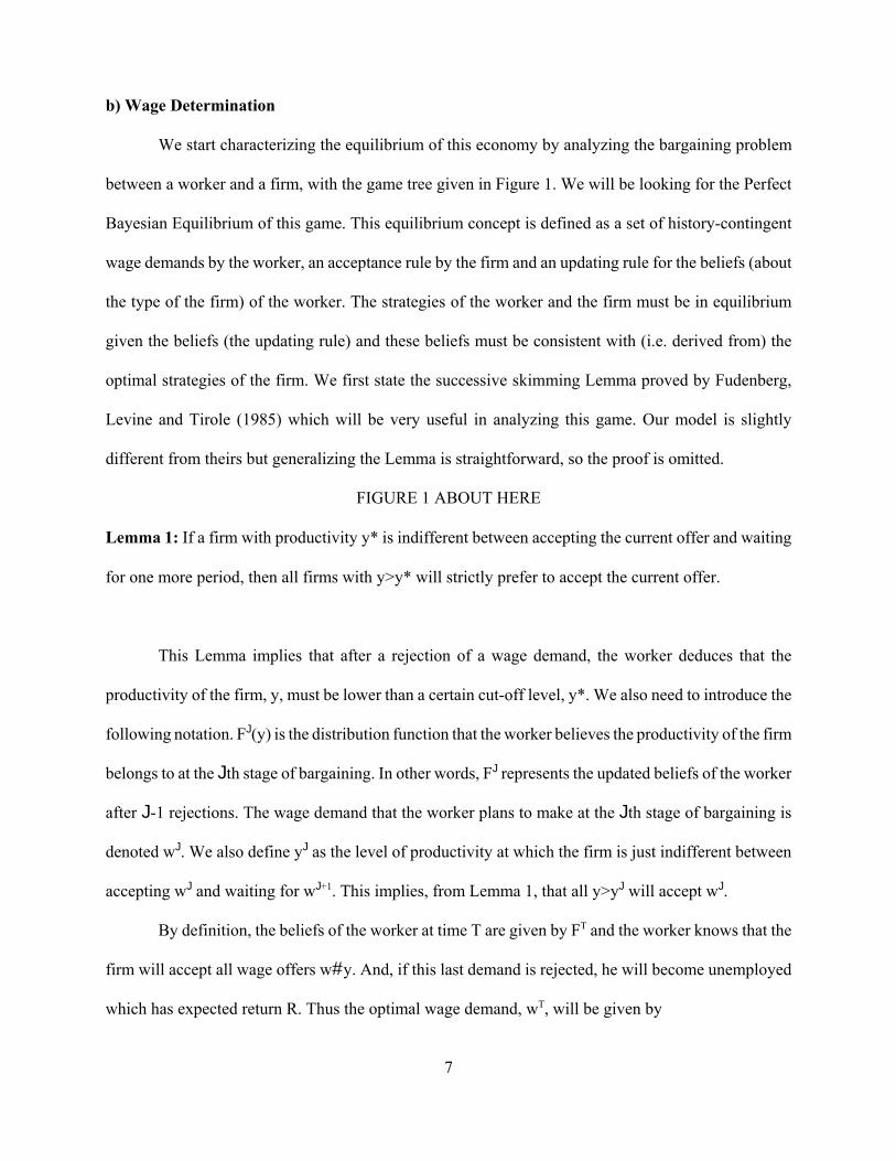
b) Wage Determination

We start characterizing the equilibrium of this economy by analyzing the bargaining problem

between a worker and a firm, with the game tree given in Figure 1. We will be looking for the Perfect

Bayesian Equilibrium of this game. This equilibrium concept is defined as a set of history-contingent

wage demands by the worker, an acceptance rule by the firm and an updating rule for the beliefs (about

the type of the firm) of the worker. The strategies of the worker and the firm must be in equilibrium

given the beliefs (the updating rule) and these beliefs must be consistent with (i.e. derived from) the

optimal strategies of the firm. We first state the successive skimming Lemma proved by Fudenberg,

Levine and Tirole (1985) which will be very useful in analyzing this game. Our model is slightly

different from theirs but generalizing the Lemma is straightforward, so the proof is omitted.

FIGURE 1 ABOUT HERE

Lemma 1: If a firm with productivity y* is indifferent between accepting the current offer and waiting

for one more period, then all firms with y>y* will strictly prefer to accept the current offer.

This Lemma implies that after a rejection of a wage demand, the worker deduces that the

productivity of the firm, y, must be lower than a certain cut-off level, y*. We also need to introduce the

following notation. FJ(y) is the distribution function that the worker believes the productivity of the firm

belongs to at the Jth stage of bargaining. In other words, FJ represents the updated beliefs of the worker

after J-1 rejections. The wage demand that the worker plans to make at the Jth stage of bargaining is

denoted wJ. We also define yJ as the level of productivity at which the firm is just indifferent between

accepting wJ and waiting for wJ+1. This implies, from Lemma 1, that all y>yJ will accept wJ.

By definition, the beliefs of the worker at time T are given by FT and the worker knows that the

firm will accept all wage offers w#y. And, if this last demand is rejected, he will become unemployed

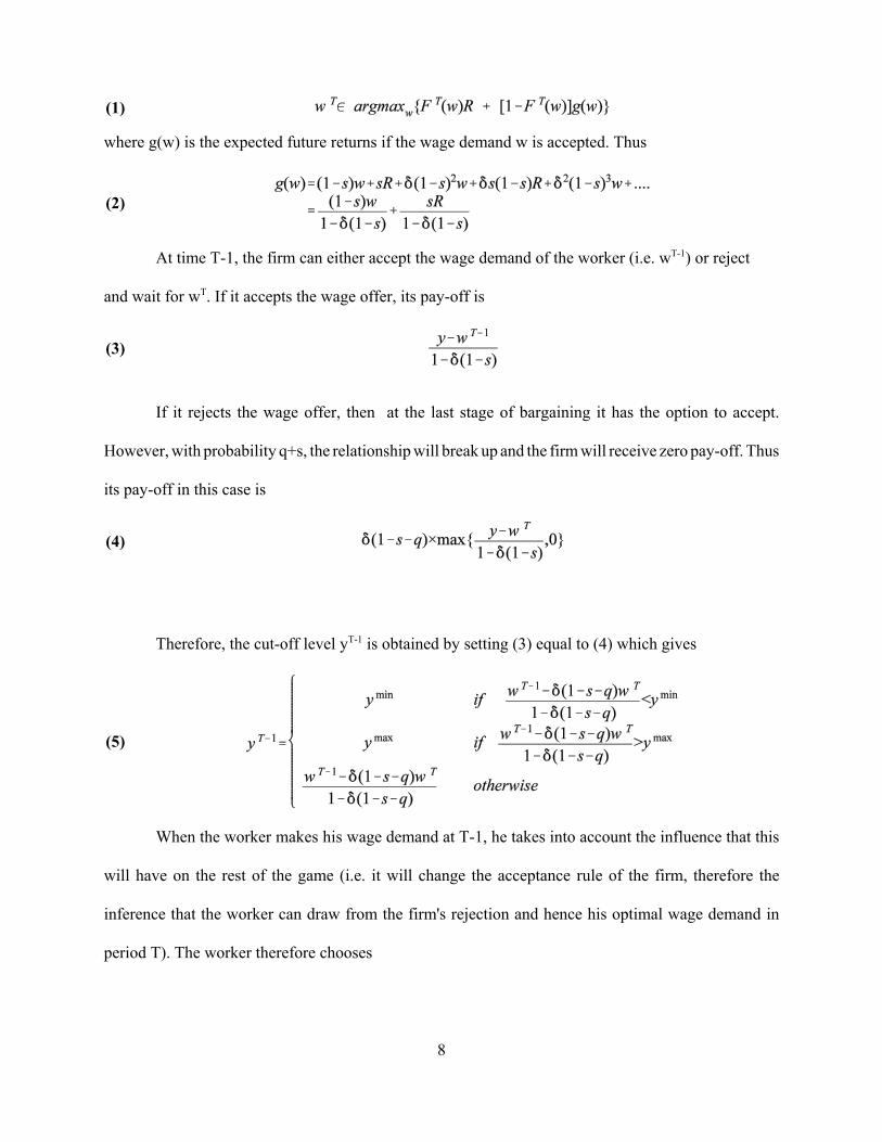
which has expected return R. Thus the optimal wage demand, wT, will be given by

8

(1)

(2)

(3)

(4)

(5)

where g(w) is the expected future returns if the wage demand w is accepted. Thus

At time T-1, the firm can either accept the wage demand of the worker (i.e. wT-1) or reject

and wait for wT. If it accepts the wage offer, its pay-off is

If it rejects the wage offer, then at the last stage of bargaining it has the option to accept.

However, with probability q+s, the relationship will break up and the firm will receive zero pay-off. Thus

its pay-off in this case is

Therefore, the cut-off level yT-1 is obtained by setting (3) equal to (4) which gives

When the worker makes his wage demand at T-1, he takes into account the influence that this

will have on the rest of the game (i.e. it will change the acceptance rule of the firm, therefore the

inference that the worker can draw from the firm's rejection and hence his optimal wage demand in

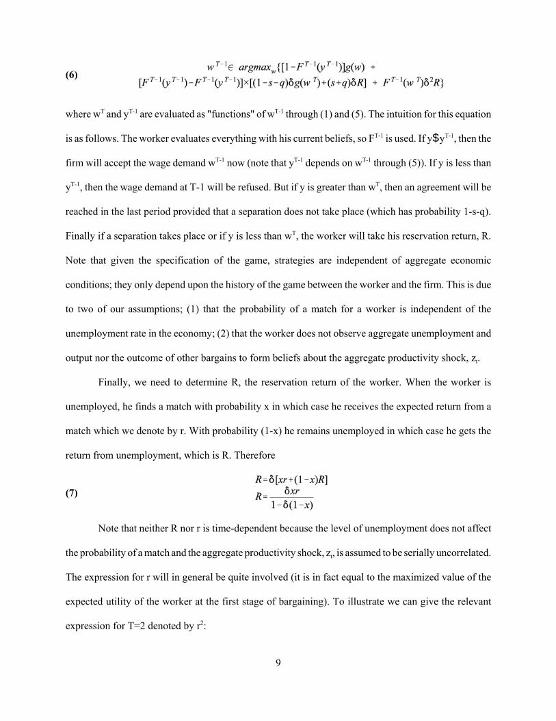
period T). The worker therefore chooses

9

(6)

(7)

where wT and yT-1 are evaluated as "functions" of wT-1 through (1) and (5). The intuition for this equation

is as follows. The worker evaluates everything with his current beliefs, so FT-1 is used. If y$yT-1, then the

firm will accept the wage demand wT-1 now (note that yT-1 depends on wT-1 through (5)). If y is less than

yT-1, then the wage demand at T-1 will be refused. But if y is greater than wT, then an agreement will be

reached in the last period provided that a separation does not take place (which has probability 1-s-q).

Finally if a separation takes place or if y is less than wT, the worker will take his reservation return, R.

Note that given the specification of the game, strategies are independent of aggregate economic

conditions; they only depend upon the history of the game between the worker and the firm. This is due

to two of our assumptions; (1) that the probability of a match for a worker is independent of the

unemployment rate in the economy; (2) that the worker does not observe aggregate unemployment and

output nor the outcome of other bargains to form beliefs about the aggregate productivity shock, zt.

Finally, we need to determine R, the reservation return of the worker. When the worker is

unemployed, he finds a match with probability x in which case he receives the expected return from a

match which we denote by r. With probability (1-x) he remains unemployed in which case he gets the

return from unemployment, which is R. Therefore

Note that neither R nor r is time-dependent because the level of unemployment does not affect

the probability of a match and the aggregate productivity shock, zt, is assumed to be serially uncorrelated.

The expression for r will in general be quite involved (it is in fact equal to the maximized value of the

expected utility of the worker at the first stage of bargaining). To illustrate we can give the relevant

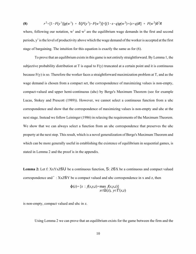
expression for T=2 denoted by r2:

10

(8)

where, following our notation, w1 and w2 are the equilibrium wage demands in the first and second

periods, y1 is the level of productivity above which the wage demand of the worker is accepted at the first

stage of bargaining. The intuition for this equation is exactly the same as for (6).

To prove that an equilibrium exists in this game is not entirely straightforward. By Lemma 1, the

subjective probability distribution at T is equal to F(y) truncated at a certain point and it is continuous

because F(y) is so. Therefore the worker faces a straightforward maximization problem at T, and as the

wage demand is chosen from a compact set, the correspondence of maximizing values is non-empty,

compact-valued and upper hemi-continuous (uhc) by Berge's Maximum Theorem (see for example

Lucas, Stokey and Prescott (1989)). However, we cannot select a continuous function from a uhc

correspondence and show that the correspondence of maximizing values is non-empty and uhc at the

next stage. Instead we follow Leininger (1986) in relaxing the requirements of the Maximum Theorem.

We show that we can always select a function from an uhc correspondence that preserves the uhc

property at the next step. This result, which is a novel generalization of Berge's Maximum Theorem and

which can be more generally useful in establishing the existence of equilibrium in sequential games, is

stated in Lemma 2 and the proof is in the appendix.

Lemma 2: Let f: XxYxZ6U be a continuous function, S: Z6X be a continuous and compact valued

correspondence and ': XxZ6Y be a compact valued and uhc correspondence in x and z, then

is non-empty, compact valued and uhc in z.

Using Lemma 2 we can prove that an equilibrium exists for the game between the firm and the

11

(9)

(10)

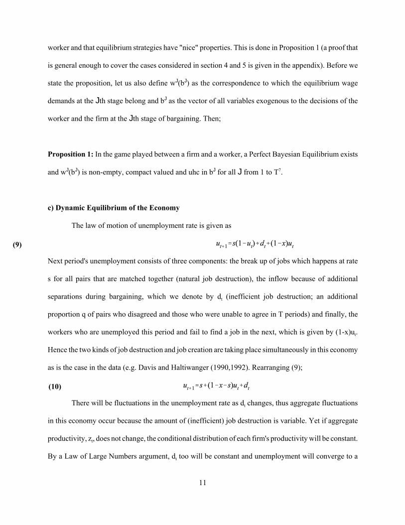
worker and that equilibrium strategies have "nice" properties. This is done in Proposition 1 (a proof that

is general enough to cover the cases considered in section 4 and 5 is given in the appendix). Before we

state the proposition, let us also define wJ(bJ) as the correspondence to which the equilibrium wage

demands at the Jth stage belong and bJ as the vector of all variables exogenous to the decisions of the

worker and the firm at the Jth stage of bargaining. Then;

Proposition 1: In the game played between a firm and a worker, a Perfect Bayesian Equilibrium exists

and wJ(bJ) is non-empty, compact valued and uhc in bJ for all J from 1 to T7.

c) Dynamic Equilibrium of the Economy

The law of motion of unemployment rate is given as

Next period's unemployment consists of three components: the break up of jobs which happens at rate

s for all pairs that are matched together (natural job destruction), the inflow because of additional

separations during bargaining, which we denote by dt (inefficient job destruction; an additional

proportion q of pairs who disagreed and those who were unable to agree in T periods) and finally, the

workers who are unemployed this period and fail to find a job in the next, which is given by (1-x)ut.

Hence the two kinds of job destruction and job creation are taking place simultaneously in this economy

as is the case in the data (e.g. Davis and Haltiwanger (1990,1992). Rearranging (9);

There will be fluctuations in the unemployment rate as dt changes, thus aggregate fluctuations

in this economy occur because the amount of (inefficient) job destruction is variable. Yet if aggregate

productivity, zt, does not change, the conditional distribution of each firm's productivity will be constant.

By a Law of Large Numbers argument, dt too will be constant and unemployment will converge to a

12

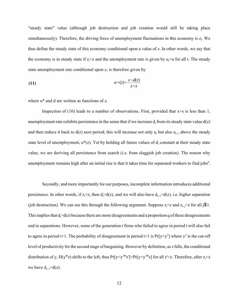
(11)

"steady state" value (although job destruction and job creation would still be taking place

simultaneously). Therefore, the driving force of unemployment fluctuations in this economy is zt. We

thus define the steady state of this economy conditional upon a value of z. In other words, we say that

the economy is in steady state if zt=z and the unemployment rate is given by ut=u for all t. The steady

state unemployment rate conditional upon z, is therefore given by

where u* and d are written as functions of z.

Inspection of (10) leads to a number of observations. First, provided that x+s is less than 1,

unemployment rate exhibits persistence in the sense that if we increase dt from its steady state value d(z)

and then reduce it back to d(z) next period, this will increase not only ut but also ut+1 above the steady

state level of unemployment, u*(z). Yet by holding all future values of dt constant at their steady state

value, we are deriving all persistence from search (i.e. from sluggish job creation). The reason why

unemployment remains high after an initial rise is that it takes time for separated workers to find jobs8.

Secondly, and more importantly for our purposes, incomplete information introduces additional

persistence. In other words, if zt<z, then dt>d(z), and we will also have dt+1>d(z), i.e. higher separation

(job destruction). We can see this through the following argument. Suppose zt<z and zt+j=z for all j$1.

This implies that dt>d(z) because there are more disagreements and a proportion q of these disagreements

end in separations. However, some of the generation t firms who failed to agree in period t will also fail

to agree in period t+1. The probability of disagreement in period t+1 is Pr[y<y2] where y2 is the cut-off

level of productivity for the second stage of bargaining. However by definition, as z falls, the conditional

distribution of y, H(y*z) shifts to the left, thus Pr[y<y2*z']>Pr[y<y2*z] for all z'<z. Therefore, after zt<z

we have dt+1>d(z).

13

The intuition for this additional persistence is as follows: the superior information of the firm is

relevant for a number of periods but in the first stage of bargaining only part of this information is

revealed, i.e. whether y is less than y1 or not. As a result, wages do not perfectly adjust to an adverse

shock leading to "dynamic wage sluggishness". Because after an adverse shock wages are higher than

they should be for a number of periods, separations (job destruction) occur at a higher rate than average.

This intuition survives beyond the specific bargaining game we have chosen to illustrate it. The crucial

requirement for incomplete information to lead to additional persistence is that agreement should take

place overtime, rather than in an instant, while agents grope towards the changed situation

The incomplete information channel of persistence is "short-lived"; after T periods there will no

longer be an effect from the realization of zt because all the information will have been revealed or

become no longer relevant. Therefore, because 1-x-s is less than 1, if zt+j=z for all j$1, the unemployment

rate will return to its steady state value and we can conclude that the steady state equilibrium of this

economy is globally stable. From the above discussion, wage demands are independent of the aggregate

level of unemployment. So wages do not fluctuate much, but are still procyclical: when zt is low,

agreements will be delayed and as wJ>wJ+1, average agreed wages will be low. When zt is low,

unemployment is high and we are in a "recession" thus giving us procyclical real wages. Yet the close

association between wages and the marginal product of labor no longer holds, making wages much less

procyclical than implied by a simple (i.e. full information and competitive) Real Business Cycle model.

In practice we can identify two channels through which wages respond to economic conditions. First,

wages may change in response to changes in the productivity of the firm and second, they may respond

to aggregate economic conditions, for example by falling when unemployment rises. The second channel

is not present as we assume the matching probability to be independent of the amount of unemployment

in the market (we allow this channel to work in the extensions). The first mechanism, on the other hand,

works only imperfectly. To see this consider the special case with T=1; the optimal wage demand will

14

be given by w=(1+R)/2 and if there is no agreement, the relationship will end. Therefore wages do not

respond to aggregate productivity, zt. However for T>1, this channel works to some extent and wages

become procyclical. Related to the delay in information revelation, it is also interesting to note that

wages lag the movement of unemployment over the cycle since they respond to information that

becomes available only slowly.

We can summarize the results of this section in Proposition 2. (The existence of steady state

equilibrium under more general conditions than here, covering the extensions of sections 4 and 5 is

provided in the Appendix).

Proposition 2: Under the assumption that x+s<1, given the equilibrium of the bargaining game, this

economy has a unique and globally stable steady state unemployment level. Unemployment, output and

wages fluctuate around this steady state in response to changes in zt. Fluctuations exhibit persistence due

to search and incomplete information effects.

d) Efficiency

Obviously, there are substantial inefficiencies in this model. Not all potentially productive

relationships are formed due to the existence of search imperfections and once a match is formed

agreement can be delayed or a separation may result because of asymmetric information. We thus say

that the economy is unable to achieve the first-best. However, it can also be asked whether a Social

Planner can improve the welfare of the agents in this economy, when she is subject to the same search

and incomplete information constraints. In our model the answer to this question is in the affirmative and

we refer to this as constrained inefficiency. There are two sources leading to this additional inefficiency.

15

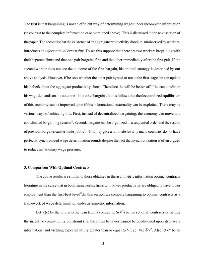
The first is that bargaining is not an efficient way of determining wages under incomplete information

(in contrast to the complete information case mentioned above). This is discussed in the next section of

the paper. The second is that the existence of an aggregate productivity shock, zt, unobserved by workers,

introduces an informational externality. To see this suppose that there are two workers bargaining with

their separate firms and that one pair bargains first and the other immediately after the first pair. If the

second worker does not see the outcome of the first bargain, his optimal strategy is described by our

above analysis. However, if he sees whether the other pair agreed or not at the first stage, he can update

his beliefs about the aggregate productivity shock. Therefore, he will be better off if he can condition

his wage demands on the outcome of the other bargain9. It thus follows that the decentralized equilibrium

of this economy can be improved upon if this informational externality can be exploited. There may be

various ways of achieving this. First, instead of decentralized bargaining, the economy can move to a

coordinated bargaining system10. Second, bargains can be organized in a sequential order and the results

of previous bargains can be made public11. This may give a rationale for why many countries do not have

perfectly synchronized wage determination rounds despite the fact that synchronization is often argued

to reduce inflationary wage pressure.

3. Comparison With Optimal Contracts

The above results are similar to those obtained in the asymmetric information optimal contracts

literature in the sense that in both frameworks, firms with lower productivity are obliged to have lower

employment than the first-best level12.In this section we compare bargaining to optimal contracts as a

framework of wage determination under asymmetric information.

Let V(c) be the return to the firm from a contract c, S(V*) be the set of all contracts satisfying

the incentive compatibility constraint (i.e. the firm's behavior cannot be conditioned upon its private

information) and yielding expected utility greater than or equal to V*, i.e. V(c)$V*. Also let c* be an

16

optimal contract in S(V*) and U(c) be the expected utility of the worker when contract c is signed. It

follows that œc0S(V*), U(c*)$U(c). We also define cb as a contract that implements a Perfect Bayesian

Equilibrium of the bargaining game. Before comparing contracts and bargaining we also need to note

that, in our analysis, we restricted the worker not to make an offer such as "You can employ me at w1

for all future periods or at w2 in alternating periods". In other words, we assumed that if the worker

works at time t, he will also work at time t+1 unless the firm becomes obsolete. If we do not impose the

same restriction on the contracts as well, they will achieve more than bargaining. However, our argument

is that there is an economically more interesting mechanism which makes bargaining less efficient. In

order to highlight this mechanism, we only allow contracts which necessarily employ the worker at t+1

if they did so at t.

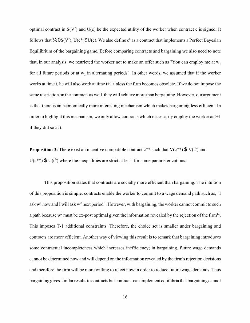
Proposition 3: There exist an incentive compatible contract c** such that V(c**) $ V(cb) and

U(c**) $ U(cb) where the inequalities are strict at least for some parameterizations.

This proposition states that contracts are socially more efficient than bargaining. The intuition

of this proposition is simple: contracts enable the worker to commit to a wage demand path such as, "I

ask w1 now and I will ask w2 next period". However, with bargaining, the worker cannot commit to such

a path because w2 must be ex-post optimal given the information revealed by the rejection of the firm13.

This imposes T-1 additional constraints. Therefore, the choice set is smaller under bargaining and

contracts are more efficient. Another way of viewing this result is to remark that bargaining introduces

some contractual incompleteness which increases inefficiency; in bargaining, future wage demands

cannot be determined now and will depend on the information revealed by the firm's rejection decisions

and therefore the firm will be more willing to reject now in order to reduce future wage demands. Thus

bargaining gives similar results to contracts but contracts can implement equilibria that bargaining cannot

17

implement, hence bargaining leads to more inefficiency and to slower revelation of information which

in our model leads to dynamic wage sluggishness and to additional persistence in unemployment. Of

course, although implicit contracts are more efficient, bargaining often arises because of the enforcement

problems associated with implicit contracts.

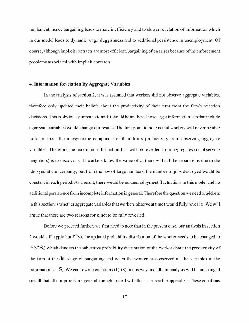
4. Information Revelation By Aggregate Variables

In the analysis of section 2, it was assumed that workers did not observe aggregate variables,

therefore only updated their beliefs about the productivity of their firm from the firm's rejection

decisions. This is obviously unrealistic and it should be analyzed how larger information sets that include

aggregate variables would change our results. The first point to note is that workers will never be able

to learn about the idiosyncratic component of their firm's productivity from observing aggregate

variables. Therefore the maximum information that will be revealed from aggregates (or observing

neighbors) is to discover zt. If workers know the value of zt, there will still be separations due to the

idiosyncratic uncertainty, but from the law of large numbers, the number of jobs destroyed would be

constant in each period. As a result, there would be no unemployment fluctuations in this model and no

additional persistence from incomplete information in general. Therefore the question we need to address

in this section is whether aggregate variables that workers observe at time t would fully reveal zt. We will

argue that there are two reasons for zt not to be fully revealed.

Before we proceed further, we first need to note that in the present case, our analysis in section

2 would still apply but FJ(y), the updated probability distribution of the worker needs to be changed to

FJ(y*St) which denotes the subjective probability distribution of the worker about the productivity of

the firm at the Jth stage of bargaining and when the worker has observed all the variables in the

information set St. We can rewrite equations (1)-(8) in this way and all our analysis will be unchanged

(recall that all our proofs are general enough to deal with this case, see the appendix). These equations

18

will give us a new level of separations at time t, dt, and the question is whether dt depends on zt

(aggregate fluctuations) and whether it depends on past values of zt (persistence in job destruction). It

is straightforward to see that if zt0St there will be no aggregate fluctuations. Next, it is also immediate

that if zt-k0St for all k>0, the relevant aggregate information is revealed immediately and the presence

of incomplete information will not lead to additional persistence. In the rest of this section we will

investigate whether under plausible conditions, St would contain current and past values of zt.

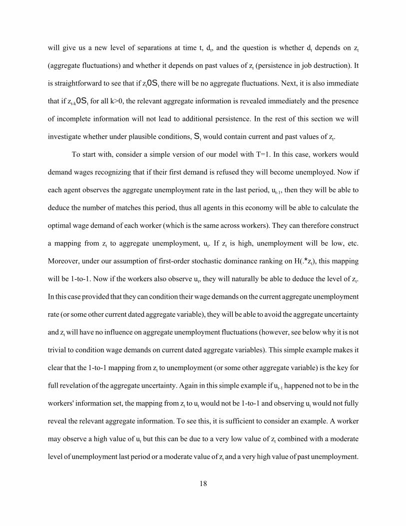
To start with, consider a simple version of our model with T=1. In this case, workers would

demand wages recognizing that if their first demand is refused they will become unemployed. Now if

each agent observes the aggregate unemployment rate in the last period, ut-1, then they will be able to

deduce the number of matches this period, thus all agents in this economy will be able to calculate the

optimal wage demand of each worker (which is the same across workers). They can therefore construct

a mapping from zt to aggregate unemployment, ut. If zt is high, unemployment will be low, etc.

Moreover, under our assumption of first-order stochastic dominance ranking on H(.*zt), this mapping

will be 1-to-1. Now if the workers also observe ut, they will naturally be able to deduce the level of zt.

In this case provided that they can condition their wage demands on the current aggregate unemployment

rate (or some other current dated aggregate variable), they will be able to avoid the aggregate uncertainty

and zt will have no influence on aggregate unemployment fluctuations (however, see below why it is not

trivial to condition wage demands on current dated aggregate variables). This simple example makes it

clear that the 1-to-1 mapping from zt to unemployment (or some other aggregate variable) is the key for

full revelation of the aggregate uncertainty. Again in this simple example if ut-1 happened not to be in the

workers' information set, the mapping from zt to ut would not be 1-to-1 and observing ut would not fully

reveal the relevant aggregate information. To see this, it is sufficient to consider an example. A worker

may observe a high value of ut but this can be due to a very low value of zt combined with a moderate

level of unemployment last period or a moderate value of zt and a very high value of past unemployment.

19

Now, observing ut is still informative but no longer fully revealing.

Next consider another example with T=2. In this case current unemployment would depend on

past level of unemployment and, the two components of job destruction: first, jobs destroyed from

current matches and second, jobs destroyed from matches of the previous period. Also suppose that

workers observe ut-1. Is ut fully revealing about zt? The answer is no because now there is no unique

mapping from zt to ut unless we condition on the amount of job destruction from the matches of the

previous period or on zt-1. This can be generalized quite simply. For the current dated aggregate variables

to be fully revealing, we need zt-k to be in the information set of all workers for all k#T-1. However, in

a dynamic world in which workers move and new entrants come to the market (and many other features

also missing from our formal model because of obvious reasons), it is a very strong assumption to

suppose that all past aggregate incomplete information problems have been solved. Thus under plausible

conditions, all past uncertainty will not have been fully revealed and this will prevent the existence of

a 1-to-1 mapping from the set of current aggregate variables to zt. This argument does not only establish

that incomplete information will cause fluctuations in our model, but also because past information has

not been fully revealed, as in our basic model, relevant information is still revealed gradually thus

incomplete information contributes to persistence in unemployment fluctuations.

An additional argument can also be made for the limited degree of information transmission.

Even when all the relevant information can be revealed by aggregate variables, for this not to have an

effect on the behavior of the aggregate economy, we need this information to be fed into the current

decision rules of agents. In the presence of a Walrasian auctioneer who coordinates trade, this is done

in a straightforward way. Each agent submits a demand schedule to the auctioneer conditional on the

realization of the aggregate variables. For instance, I demand the wage w1 if aggregate unemployment

is u1 but a different wage w2 if the aggregate unemployment rate is u2. However, the distinguishing

feature of our economy is that the auctioneer does not exist. Each agent has to make a wage demand and

20

it is only as a result of these wage demands that the aggregate unemployment level is determined. In the

absence of a coordinating agent, it is not possible to condition current wage demands on the current

realization of the unemployment rate. This is because for the aggregate unemployment rate to be

determined, the firms first have to decide whether they accept the wage demands of their workers;

therefore the exact wage demands of the workers need to be determined first. Consequently in general

the relevant information will only be fed into decision rules with some delay, thus the transmission of

information will be slowed down.

This idea can be formalized in a very simple way. We can define a relation P such that aPb

means a precedes b where a and b refer to decisions by distinct set of agents in the economy. "Precede"

in this context means that decision a can be condition upon the realization of decision b. In a centralized

trading system such as a market coordinated by a Walrasian auctioneer, P does not need to be anti-

symmetric; aPb and bPa can be simultaneously true since the auctioneer can determine both at the same

time. Unemployment is only determined from individual decision rules but individual decision rules can

be conditioned upon the unemployment rate of the same period because agents can submit schedules that

map the aggregate unemployment rate (and other aggregate variables) to their decisions and the

auctioneer finds a general equilibrium as a fixed point vector of all these decision rules. However, in an

environment without an auctioneer, this procedure does not seem plausible and motivated by this, we

define a decentralized trading system as an environment in which P is anti-symmetric for any two

arguments that refer to different sets of agents. If aPb, then bPa cannot be true. Now in our example take

"a" to be individual decisions and "b" to be the aggregate unemployment rate, thus aPb must be true since

without knowing the individual decision rules we cannot determine how many separations will occur.

Thus it is impossible at the same time to condition individual agreements on the current unemployment

rate. Therefore, the current decision rules of workers and firms can only depend on the realization of the

past unemployment rate. These considerations will further limit the degree to which relevant information

21

(12)

(13)

(14)

will be revealed and more importantly will be used by the agents in the decentralized equilibrium.

Overall we can argue that under plausible conditions, not all the relevant aggregate information

will be revealed and fed into decisions rules in an economy like ours and the effects discussed in section

2 will survive even in the presence of larger information sets than considered there.

5. Extensions

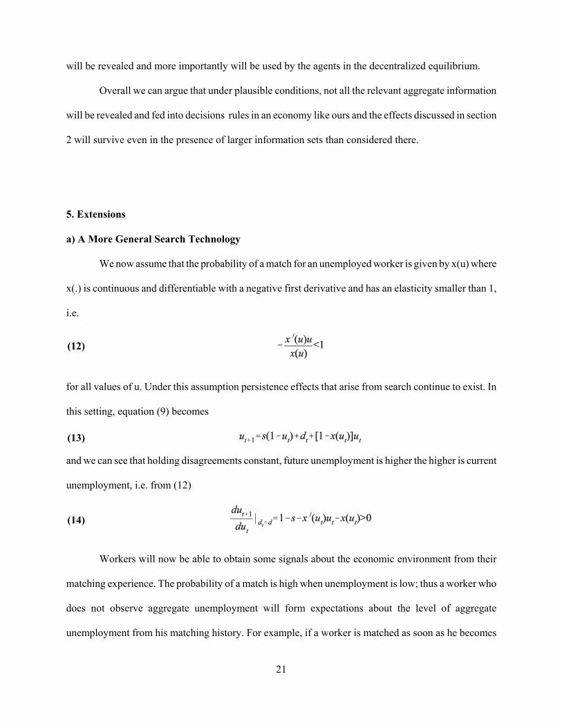
a) A More General Search Technology

We now assume that the probability of a match for an unemployed worker is given by x(u) where

x(.) is continuous and differentiable with a negative first derivative and has an elasticity smaller than 1,

i.e.

for all values of u. Under this assumption persistence effects that arise from search continue to exist. In

this setting, equation (9) becomes

and we can see that holding disagreements constant, future unemployment is higher the higher is current

unemployment, i.e. from (12)

Workers will now be able to obtain some signals about the economic environment from their

matching experience. The probability of a match is high when unemployment is low; thus a worker who

does not observe aggregate unemployment will form expectations about the level of aggregate

unemployment from his matching history. For example, if a worker is matched as soon as he becomes

22

unemployed, he will deduce that the unemployment rate, ut, is low and, judging his reservation return

relatively high, will make higher wage demands. On the other hand a worker who receives no matches

for a few periods will believe unemployment to be high and will make more moderate wage demands

upon being matched with a firm. Also, as unemployment now affects matching probabilities and so

outside opportunities, the second channel, mentioned in section 2(d), through which aggregate economic

conditions influence wages will function, albeit only imperfectly. In the appendix, we prove that a steady

state equilibrium exists, with this general search technology (as well as when a vector of aggregate

variables, kt, is in the information set of the workers)14.

b) Infinite Horizon Bargaining With Outside Options

The assumptions on the bargaining game used in section 2 were quite restrictive. First, we

imposed an end-period to the bargaining game. Second, we have not allowed the worker to opt out of

the relationship and join the unemployment pool. Although these assumptions considerably simplified

the analysis and the exposition, it will be instructive to investigate whether any of our results have

specifically followed from these. A more natural bargaining game to analyze would be one where the

horizon is infinite and the worker can choose to take his outside option at any stage. This is the game that

we will discuss in this section. We will see that the equilibrium of the present game is the same as the

equilibrium of the game analyzed in section 2, when T is chosen appropriately.

Rather than solve this game fully we will borrow from the analysis of Fudenberg, Levine and

Tirole (1987). Also for simplification, we set q=s=0 and take R constant as in section 2. Two results that

are important for us follow from their analysis:

(1) There exist multiple equilibria.

(2) As long as R>g(ymin), at some point, the worker will become sufficiently pessimistic and quit the

relationship.

23

The existence of multiple equilibria poses some problems as well as raise some interesting issues.

It can be asked whether shifts in the relevant equilibrium do contribute to the cyclical fluctuations of the

economy. This is certainly possible but there is not much we can say about it either. A more natural

approach would be to suppose that once one of the possible equilibria is chosen, a change of equilibrium

thereafter is unlikely. However, point (2) above implies that once we are in one of these equilibria, the

firm and the worker will bargain up to a point until which the outside option is not exercised and at that

point the worker switches. Thus we can call this point T and the qualitative results from all of these

equilibria are the same as our basic model analyzed in section 2, with the difference that T is now

endogenously determined15.

6. Conclusion

We have analyzed a dynamic general equilibrium in which wages are determined through

bargaining. Because the firm has superior information, delays and inefficient separations lead to output

and employment fluctuations. This persistence of fluctuations is derived from the incomplete information

channel which introduces "dynamic wage sluggishness", as well as the more conventional search

channel. A feature of this dynamic wage sluggishness compared to conventional channels of persistence

is that it implies persistence in job destruction not only in job creation.

Our model has close links with the RBC models such as Kydland and Prescott (1982) and Long

and Plosser (1983) since we are concerned with the dynamics of the aggregate economy in response to

an exogenous driving force. However, the economic and persistence mechanisms are different and the

presence of missing markets breaks the link between real wages and the marginal product of labour. This

reduces real wage fluctuations while increasing the cyclical variability of employment. Missing markets

also make the equilibrium inefficient. Further, given the informational and technological restrictions, a

Social Planner can still improve upon the decentralized equilibrium by exploiting the informational

24

externalities that are present. We have also emphasized the similarity of our results to optimal contracts

and shown that bargaining is a less efficient way of wage and employment determination. However, it

may nevertheless arise because of enforceability problems associated with complicated implicit

contracts.

As our model was mainly concerned with economic and persistence mechanisms derived from

incomplete information bargaining embedded in a dynamic general equilibrium model, we have not

discussed the driving force of the cycle in great detail and interpreted it as a common productivity shock.

However, the same set-up can be used to generate economic fluctuations in response to real demand

shocks or even changes in "animal spirits" as long as all the effects are not in everyone's information set.

In particular, the persistence channel provided by incomplete information may be important in explaining

the sluggish response of the real economy to unanticipated demand shocks.

25

(A1)

(A2)

Appendix

Proof of Lemma 2: Take an arbitrary z. A function y=h(x,z), upper semi-continuous (usc) in x can

always be selected from '(x,z). Let g(x,z)=f(x,h(x,z),z). Then g(x,z) is usc in x and x belongs to the

continuous and compact valued correspondence S(z), therefore a maximum exists and N(z) is non

empty.

Now take zn6z, xn0N(zn) and xn6x. By definition, there exists yn0'(xn,zn) such that

' is uhc in x and z, therefore, there exists y0'(x,z) such that yn6y. Thus take limits in (1A) and use the

continuity of f, we have:

Therefore, x0N(z) and N is uhc in z.

Finally, NfS and S is compact so N is bounded. Also, take xn6x and xn0N(z). By the above

argument, lim f(xn,yn,z)=f(x,y,z) as f is continuous and x0N(z) and N is closed, therefore compact

valued. As z was arbitrary N is non-empty, uhc and compact valued for all z. QED

Proof of Proposition 1: At T the worker maximizes (1) in the text choosing w from the non-empty

compact set [yT-1,ymax]. From Lemma 1, FT is continuous in yT-1 (and trivially in wT-1,

yT-2,... since it does not directly depend on these). Therefore, the correspondence to which maximizers

of (1) belong to, wT(bT), is non-empty, compact valued and uhc in bT=(yT-1, wT-1, yT-2,....., R) by Berge's

Maximum Theorem. Equation (5) in the text gives yT-1 as a function of wT-1 and wT, thus we can

substitute this function in wT(bT) and obtain a non-empty and compact-valued correspondence, NT, which

is also uhc in wT-1, yT-2, wT-2, ..... and R. At T-1 the worker maximizes (6) which is continuous in wT, wT-1,

yT-1 and R choosing wT from the set [yT-2,ymax] and wT-1 from the set [yT-1,ymax] subject to (1) and (5). We

can substitute from (5) for yT-1 and as (5) is continuous the function to be maximized is continuous in wT,

26

(A3)

(A4)

yT-2, wT-1, ... and R and it is subject to the constraint that wT-1,NT(yT-2, wT-2, ..., R) defined above.

Therefore Lemma 2 implies that wT-1(bT-1) is non-empty, compact valued and uhc in bT-1=(yT-2, wT-2,.....,

R). We can repeat this argument recursively and conclude that wJ(bJ) is non-empty and that it is compact

valued and uhc in bJ for all J. The fact that the optimal strategy correspondence is non-empty also

implies that an equilibrium exists. QED

Proof of Proposition 3: The optimal contract is chosen as a result of a maximization problem subject

to incentive compatibility constraints and subject to the restriction that the firm gets a certain level of

utility. Thus if we denote the maximand by G(w1, w2, ....., wT), the optimal contract, c*, is chosen as T

wages {w1c, w2c,...., wTc} such that

subject to T-1 incentive compatibility constraints which take the form of equations similar to (5) in the

text and that V(c*)$V*. However from the proof of Proposition 1, the solution of the bargaining problem

is given by maximizing (A3) subject to the above constraints and T-1 additional constraints

for J=2,....,T, which say that future wage demands must be ex post optimal for the worker given the

information revealed by the rejection decisions of the firm, e.g. (1) in the text.

Therefore defining the set of contracts to which cb belongs to as Sb, we can see that SbdS(V(cb)),

where, by definition, the firm gets return V(cb) in the equilibrium of the bargaining game and strict

inclusion holds because of the T-1 additional constraints. For the optimal contract in S(V(cb)), c*, it is

true that U(c*)$U(c), œc0S(V(cb)), therefore V(c*)$V(cb). Because of the strict inclusion, the

inequalities will be strict at least for some problems16. Therefore, we can always find c** such that

V(c**)$V(cb) and U(c**)$U(cb) and the strict inequalities will hold at least for some parameterizations.

QED

27

(A5)

(A6)

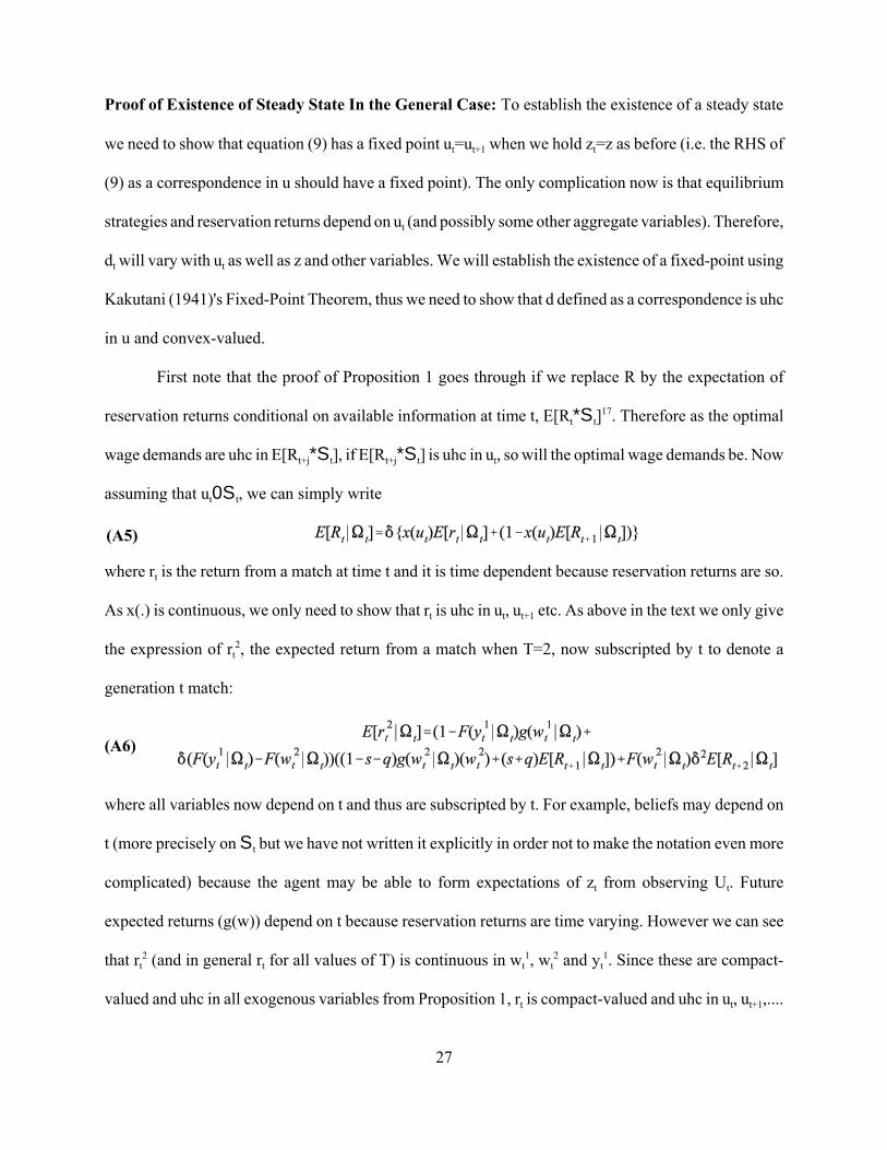
Proof of Existence of Steady State In the General Case: To establish the existence of a steady state

we need to show that equation (9) has a fixed point ut=ut+1 when we hold zt=z as before (i.e. the RHS of

(9) as a correspondence in u should have a fixed point). The only complication now is that equilibrium

strategies and reservation returns depend on ut (and possibly some other aggregate variables). Therefore,

dt will vary with ut as well as z and other variables. We will establish the existence of a fixed-point using

Kakutani (1941)'s Fixed-Point Theorem, thus we need to show that d defined as a correspondence is uhc

in u and convex-valued.

First note that the proof of Proposition 1 goes through if we replace R by the expectation of

reservation returns conditional on available information at time t, E[Rt*St]17. Therefore as the optimal

wage demands are uhc in E[Rt+j*St], if E[Rt+j*St] is uhc in ut, so will the optimal wage demands be. Now

assuming that ut0St, we can simply write

where rt is the return from a match at time t and it is time dependent because reservation returns are so.

As x(.) is continuous, we only need to show that rt is uhc in ut, ut+1 etc. As above in the text we only give

the expression of rt2, the expected return from a match when T=2, now subscripted by t to denote a

generation t match:

where all variables now depend on t and thus are subscripted by t. For example, beliefs may depend on

t (more precisely on St but we have not written it explicitly in order not to make the notation even more

complicated) because the agent may be able to form expectations of zt from observing Ut. Future

expected returns (g(w)) depend on t because reservation returns are time varying. However we can see

that rt2 (and in general rt for all values of T) is continuous in wt

1, wt2 and yt

1. Since these are compact-

valued and uhc in all exogenous variables from Proposition 1, rt is compact-valued and uhc in ut, ut+1,....

28

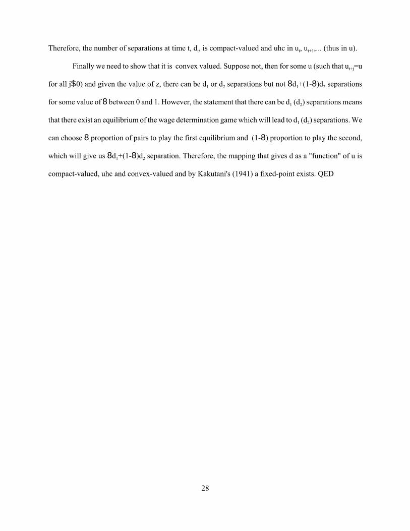
Therefore, the number of separations at time t, dt, is compact-valued and uhc in ut, ut+1,... (thus in u).

Finally we need to show that it is convex valued. Suppose not, then for some u (such that ut+j=u

for all j$0) and given the value of z, there can be d1 or d2 separations but not 8d1+(1-8)d2 separations

for some value of 8 between 0 and 1. However, the statement that there can be d1 (d2) separations means

that there exist an equilibrium of the wage determination game which will lead to d1 (d2) separations. We

can choose 8 proportion of pairs to play the first equilibrium and (1-8) proportion to play the second,

which will give us 8d1+(1-8)d2 separation. Therefore, the mapping that gives d as a "function" of u is

compact-valued, uhc and convex-valued and by Kakutani's (1941) a fixed-point exists. QED

29

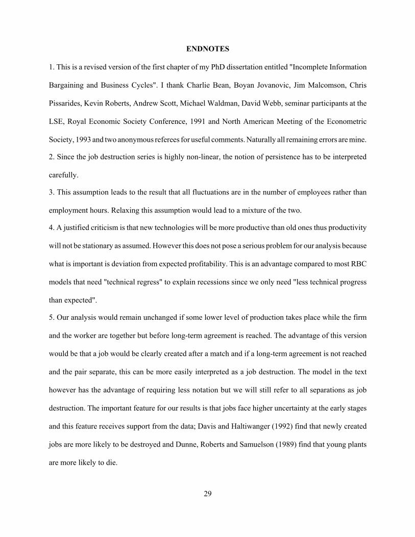
1. This is a revised version of the first chapter of my PhD dissertation entitled "Incomplete Information

Bargaining and Business Cycles". I thank Charlie Bean, Boyan Jovanovic, Jim Malcomson, Chris

Pissarides, Kevin Roberts, Andrew Scott, Michael Waldman, David Webb, seminar participants at the

LSE, Royal Economic Society Conference, 1991 and North American Meeting of the Econometric

Society, 1993 and two anonymous referees for useful comments. Naturally all remaining errors are mine.

2. Since the job destruction series is highly non-linear, the notion of persistence has to be interpreted

carefully.

3. This assumption leads to the result that all fluctuations are in the number of employees rather than

employment hours. Relaxing this assumption would lead to a mixture of the two.

4. A justified criticism is that new technologies will be more productive than old ones thus productivity

will not be stationary as assumed. However this does not pose a serious problem for our analysis because

what is important is deviation from expected profitability. This is an advantage compared to most RBC

models that need "technical regress" to explain recessions since we only need "less technical progress

than expected".

5. Our analysis would remain unchanged if some lower level of production takes place while the firm

and the worker are together but before long-term agreement is reached. The advantage of this version

would be that a job would be clearly created after a match and if a long-term agreement is not reached

and the pair separate, this can be more easily interpreted as a job destruction. The model in the text

however has the advantage of requiring less notation but we will still refer to all separations as job

destruction. The important feature for our results is that jobs face higher uncertainty at the early stages

and this feature receives support from the data; Davis and Haltiwanger (1992) find that newly created

jobs are more likely to be destroyed and Dunne, Roberts and Samuelson (1989) find that young plants

are more likely to die.

ENDNOTES

30

6. Naturally, this story makes more sense when firms sell non-homogenous products but it is assumed,

for simplicity, that all products are homogenous.

7. We can also see from the proof of Proposition 1 that the backward induction that describes the Perfect

Bayesian Equilibrium of this game is unique. However this does not guarantee uniqueness of the

equilibrium because a maximization problem such as (1) or (6) may have multiple solutions. Fudenberg,

Levine and Tirole (1985) have shown that in the infinite horizon version of this game without reservation

returns and with some restrictions on the distribution function, the equilibrium is generically unique.

8. It is useful to note that although this channel of persistence is not related to the asymmetry of

information, in this model there would be no unemployment fluctuations if information were complete.

Thus, the incompleteness of information is the source of all unemployment fluctuations.

9. This will be achieved to some extent when we allow workers to observe aggregate unemployment and

output but not perfectly.

10. In section 5(b) we will argue that observed variables will not transmit much information about

current dated variables because of the absence of a coordinating agent. To have coordinating bargaining

can be in this context recognized as introducing such an agent.

11. The technical details of this argument are developed in section IV of Acemoglu (1992). It has to be

noted that this system would not internalize all the effects of the informational externality and a similar

inefficiency to those encountered in the herding models (e.g. Banerjee 1992) will remain.

12. The contracts we have mind are such that the worker and the firm get together at t=0, and determine

a complete schedule of wage and employment levels (or probabilities). The firm chooses a particular

point on this schedule after finding out about its productivity. For details, see Grossman and Hart (1983),

Hart (1983). All the contracts we refer to are assumed to be enforceable.

13. So far, we have assumed that enforceable contracts could be written after the bargain, motivated by

the observation that once agreement is reached the worker and the firm enter a long-term relationship

31

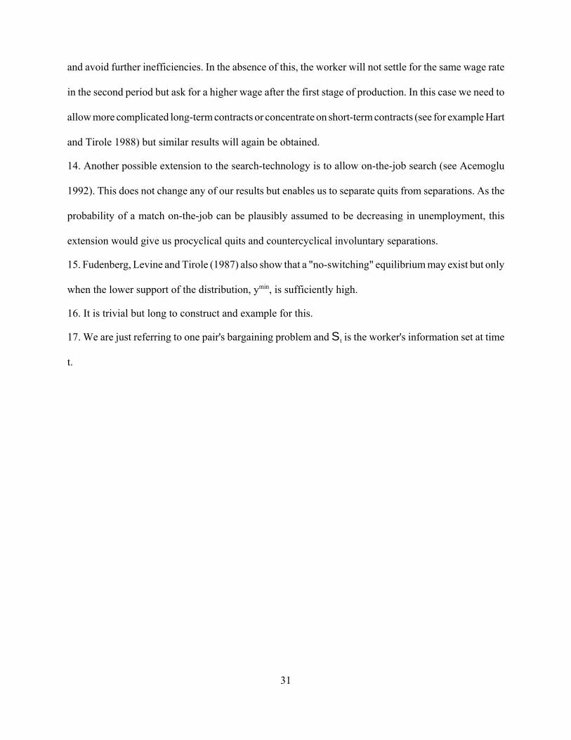
and avoid further inefficiencies. In the absence of this, the worker will not settle for the same wage rate

in the second period but ask for a higher wage after the first stage of production. In this case we need to

allow more complicated long-term contracts or concentrate on short-term contracts (see for example Hart

and Tirole 1988) but similar results will again be obtained.

14. Another possible extension to the search-technology is to allow on-the-job search (see Acemoglu

1992). This does not change any of our results but enables us to separate quits from separations. As the

probability of a match on-the-job can be plausibly assumed to be decreasing in unemployment, this

extension would give us procyclical quits and countercyclical involuntary separations.

15. Fudenberg, Levine and Tirole (1987) also show that a "no-switching" equilibrium may exist but only

when the lower support of the distribution, ymin, is sufficiently high.

16. It is trivial but long to construct and example for this.

17. We are just referring to one pair's bargaining problem and St is the worker's information set at time

t.

32

REFERENCES

Acemoglu, D. (1992);"Incomplete Information Bargaining and Business Cycles" Centre For Economic

Performance, Discussion Paper No. 60.

Banerjee, A. (1992);"A Simple Model of Herd Behavior" Quarterly Journal of Economics Vol 107, pp

797-819.

Blanchard, O. J. and P. A. Diamond (1990);"The Cyclical Behavior of the Gross Flows of US Workers"

Brookings Papers on Economic Activity Vol 2, pp 85-155.

Blanchard, O. J. and L. Summers (1986);"Hysteresis and the European Unemployment Problem" in S.

Fischer ed. NBER Macroeconomic Annual 1986, MIT Press.

Caballero R. and M. Hammour (1994);"The Timing and Efficiency of Job Creation and Destruction"

MIT Mimeo.

Davis, S. and J. Haltiwanger (1990);"Gross Job Creation and Destruction: Microeconomic Evidence and

Macroeconomic Implications" NBER Macroeconomic Annual, Vol 5, pp 123-168.

Davis, S. and J. Haltiwanger (1992);"Gross Job Creation, Gross Job Destruction and Employment

Reallocation" Quarterly Journal of Economics Vol 107, pp 819-864.

Dunne, T., M. Roberts and L. Samuelson (1989);"The Growth and Failure of US Manufacturing Plants"

Quarterly Journal of Economics Vol 104, pp 671-698.

Fudenberg, D., D. Levine and J. Tirole (1985);"Infinite Horizon Models of Bargaining With One-Sided

Incomplete Information" in A. Roth(ed) Game Theoretic Models of Bargaining Cambridge University

Press.

Fudenberg, D., D. Levine and J. Tirole (1987);"Incomplete Information Bargaining with Outside

Options" Quarterly Journal of Economics Vol 102, pp 37-50.

Grossman, S. and O. Hart (1983);"Implicit Contracts under Asymmetric Information" Quarterly Journal

of Economics Vol 98.

33

Grossman, S., O. Hart and E. Maskin (1983);"Unemployment with Observable Aggregate Shocks"

Journal of Political Economy Vol 91, pp 907-928

Hart, O. (1983);"Optimal Labour Contracts Under Asymmetric Information: An Introduction" Review

of Economic Studies Vol 50, pp 3-35.

Hart, O. (1989);"Bargaining and Strikes" Quarterly Journal of Economics Vol 54, pp 25-45.

Hart, O. and J. Tirole (1988);"Contract Renegotiation and Coasian Dynamics" Review of Economic

Studies Vol 55, pp 509-540.

Jaeger A. and M. Parkinson (1994);"Some Evidence on the Hysteresis of Unemployment Rates"

European Economic Review Vol 38, pp 329-342.

Kakutani, S. (1941);"A Generalization of Brouwer's Fixed-Point Theorem" Duke Mathematical \Journal

Vol 3, pp 457-459.

Kydland, F. and E. Prescott(1982);"Time to Build and Aggregate Fluctuations" Econometrica Vol 50,

pp 1345-1371.

Leininger, W. (1986); "The Existence of Perfect Equilibria in a Model of Growth with Altruism between

Generations" Review of Economic Studies Vol 53, pp 349-367.

Lindbeck A. and D. Snower (1988); The Insider-Outsider Theory of Employment and Unemployment,

Cambridge, MIT Press.

Long, J. B. and C. I. Plosser (1983);"Real Business Cycles" Journal of Political Economy, Vol 91, pp

1345-1370.

Mortensen, D. T. and C. A. Pissarides (1994);"Job Creation and Job Destruction in the Theory of

Unemployment" Review of Economic Studies Vol 61, pp 397-416.

Perry, M. and G. Solon (1985);"Wage Bargaining, Labour Turnover and the Business Cycles: A Model

with Asymmetric Information" Journal of Labor Economics Vol 3.

Pissarides, C. A. (1985);"Short-run Equilibrium Dynamics of Unemployment, Vacancies and Real

34

Wages" American Economic Review Vol 75, pp 676-690.

Smith, B (1989); "A Business Cycle Model with Private Information" Journal of Labor Economics Vol

7, pp 210-237.

Stokey, N., R. Lucas and E. Prescott (1989); Recursive Methods in Economic Dynamics, Cambridge,

Harvard University Press.

Wright, R. (1986);"Job Search and Cyclical Unemployment" Journal of Political Economy, Vol 94, 38-

55.

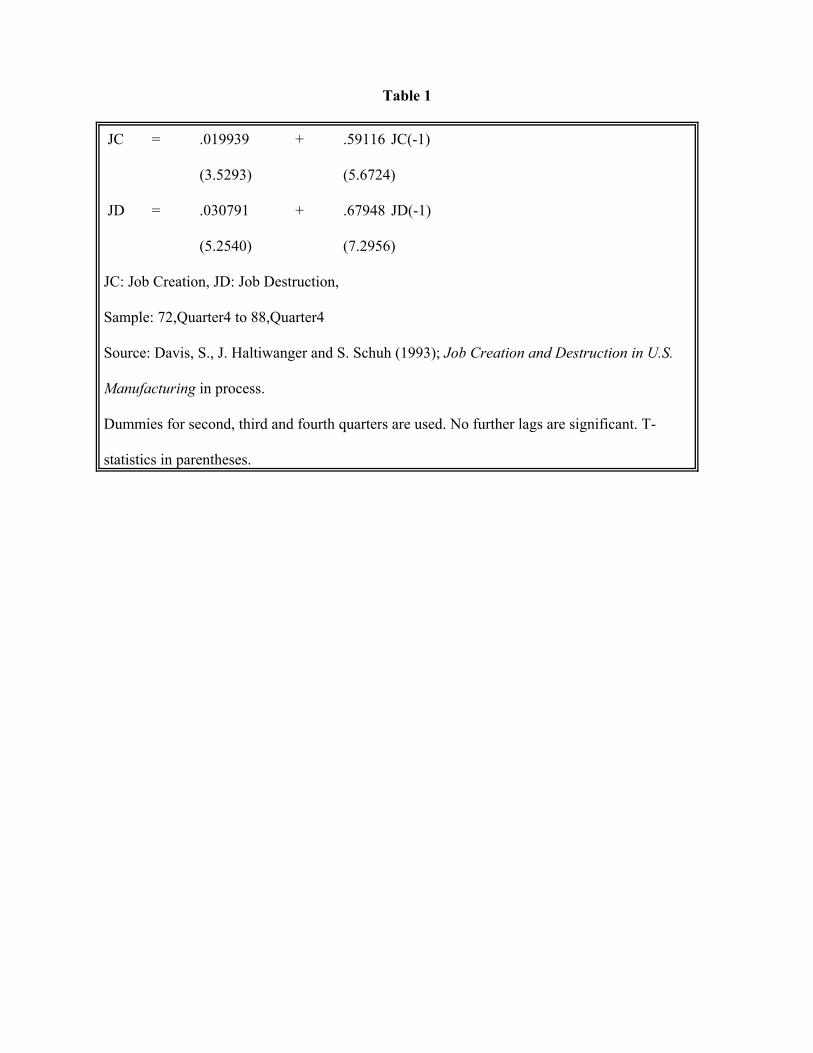
Table 1

JC = .019939 + .59116 JC(-1)

(3.5293) (5.6724)

JD = .030791 + .67948 JD(-1)

(5.2540) (7.2956)

JC: Job Creation, JD: Job Destruction,

Sample: 72,Quarter4 to 88,Quarter4

Source: Davis, S., J. Haltiwanger and S. Schuh (1993); Job Creation and Destruction in U.S.

Manufacturing in process.

Dummies for second, third and fourth quarters are used. No further lags are significant. T-

statistics in parentheses.