Embed Size (px)
Citation preview

1
Asymmetric Behavior of Inflation Uncertainty and
Friedman-Ball Hypothesis: Evidence from Pakistan
Syed Kumail Abbas Rizvi‡
Abstract
This paper is first attempt to measure and analyze inflation uncertainty in Pakistan and
it provides several contributions. Using quarterly data from 1976:01 to 2008:02, at first
stage we model inflation uncertainty as time varying process through GARCH
framework. At second stage asymmetric behavior of inflation uncertainty is analyzed by
using GJR-GARCH and EGARCH models, for further analysis of asymmetry and leverage
effects, we developed news impact curves proposed by Pagan and Schwart (1990).
Finally we investigate the causality and its direction between inflation and inflation
uncertainty by using bivariate Granger-Causality test to know which inflation
uncertainty hypothesis (Friedman-Ball or Cukierman-Meltzer) holds true for Pakistani
data.
We get two important results. First, GJR-GARCH and EGARCH models are more
successful in capturing inflation uncertainty and its asymmetric behavior as compared
to simple GARCH model. This can also be seen from news impact curves. Second, there is
strong evidence that Friedman-Ball inflation uncertainty hypothesis holds true for
Pakistan.
Keywords: Inflation, Uncertainty, GJR-GARCH, EGARCH, Friedman-Ball hypothesis
JEL Classification: C22, E31, E37
‡ Doctoral Student at TEAM laboratories, University of Paris I (Panthéon Sorbonne).
I am grateful to Prof. Christian Bordes (Université Paris 1) for his continuous guidance at the
various stages of the research that eventually helped me to bring this paper in its final shape. I
would also like to thank Prof. Philippe Rous (Université de Limoges) and Prof. Samuel
Maveyraud (Université Montesquieu - Bordeaux IV) for their detailed comments and valuable
suggestions, which greatly improved the quality of this research.

2
Introduction:
Inflation is undoubtedly one of the most largely observed and tested economic variable
both theoretically and empirically. Its causes, impacts on other economic variables and
cost to the overall economy are well known and understood. One cannot say with
certainty whether the Inflation is good or bad for an economy but if the debate focuses
on inflation uncertainty or inflation variability instead of just inflation, economists have
almost consensus about its negative impact over some of the most important economic
variables, like output and growth rate via different channels.
Inflation uncertainty is considered as one of the major cost of Inflation as it not only
distort the decisions regarding the future saving and investment due to less
predictability of real value of future nominal payments, but also extends the adverse
affects of these distortions on the efficiency of resource allocation and the level of real
activity. (Fischer 1981, Golob 1993, Holland 1993b).
One can divide the consequences of Inflation uncertainty in two categories, Ex-ante
consequences and Ex-Post consequences. Ex-ante consequences are primarily based
upon decisions in which an economic agent rationally anticipate about future inflation
and its transmission can be performed via three different channels; Financial market
Channel where Inflation uncertainty makes Investment in long tem debt more riskier
which increases expected return and long term interest rates. High long term interest
rate reduces Investment in both Business and Household sector via reduction in
investment in Plant & Equipment and Housing & Durable goods. Second channel is
Decision Variables Channel where Inflation uncertainty leads to uncertainty about
interest rate and other economic variables, due to which economic agents would not be
able to index contractual payments according to Inflation, which in turn increases
uncertainty about wages, rent, taxes, depreciation and profits and firms will be forced to
delay their hiring, production and mainly investment because these decisions are

3
unlikely to reverse, thus reducing the overall economic activity. Third channel is
Productive vs. Protective Strategies channel where Inflation uncertainty forced firms to
shift their allocation of resources from more productive to less productive uses such as
improved forecast about inflation and hedging activities via derivatives to cop up
increased uncertainty. Firm’s resources will divert from productive strategies to
protective actions which are more costly for small enterprises and households (Golob
1994). Ex-post effects of inflation uncertainty include transfer of wealth due to under or
over valuation of real payments versus nominal payments which disturbs the status quo
between Employer and Employee, Lender and borrower. (Blanchard 1997)
However, the relationship between Inflation and Inflation uncertainty is still debatable
as high inflation cause uncertainty or uncertainty cause high inflation. Friedman (1977)
was the first who formalized the relationship between Inflation and Inflation
Uncertainty and he strongly supported the causality running from inflation to inflation
uncertainty which is generally known as Friedman-Ball Hypothesis. This hypothesis has
also been extensively studied by many authors and the overall results are mixed. Ball
and Cecchetti (1990), Cukierman and Wachtel (1979), Evans (1991), and Grier and
Perry (1998), among others, provide evidence in support of a positive impact of the
average rate of inflation on inflation uncertainty. Grier and Perry (1998) found that in all
G7 countries inflation has a significant and positive effect on inflation uncertainty.
Hafer(1985) also tested the Friedman’s hypothesis that high inflation uncertainty leads
to higher level of unemployment, lower level of output and slower growth in
employment, by considering standard deviation of quarterly inflation forecasts obtained
through the ASA-NBER survey of professional forecasters, as a proxy for Inflation
uncertainty.
On the other hand the causality running in opposite direction from Inflation uncertainty
to Inflation can be considered as Cukierman-Meltzer hypothesis. (Cukierman-Meltzer
4
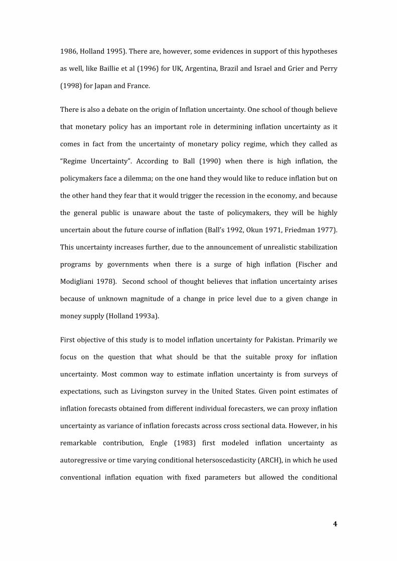
1986, Holland 1995). There are, however, some evidences in support of this hypotheses
as well, like Baillie et al (1996) for UK, Argentina, Brazil and Israel and Grier and Perry
(1998) for Japan and France.
There is also a debate on the origin of Inflation uncertainty. One school of though believe
that monetary policy has an important role in determining inflation uncertainty as it
comes in fact from the uncertainty of monetary policy regime, which they called as
“Regime Uncertainty”. According to Ball (1990) when there is high inflation, the
policymakers face a dilemma; on the one hand they would like to reduce inflation but on
the other hand they fear that it would trigger the recession in the economy, and because
the general public is unaware about the taste of policymakers, they will be highly
uncertain about the future course of inflation (Ball’s 1992, Okun 1971, Friedman 1977).
This uncertainty increases further, due to the announcement of unrealistic stabilization
programs by governments when there is a surge of high inflation (Fischer and
Modigliani 1978). Second school of thought believes that inflation uncertainty arises
because of unknown magnitude of a change in price level due to a given change in
money supply (Holland 1993a).
First objective of this study is to model inflation uncertainty for Pakistan. Primarily we
focus on the question that what should be that the suitable proxy for inflation
uncertainty. Most common way to estimate inflation uncertainty is from surveys of
expectations, such as Livingston survey in the United States. Given point estimates of
inflation forecasts obtained from different individual forecasters, we can proxy inflation
uncertainty as variance of inflation forecasts across cross sectional data. However, in his
remarkable contribution, Engle (1983) first modeled inflation uncertainty as
autoregressive or time varying conditional hetersoscedasticity (ARCH), in which he used
conventional inflation equation with fixed parameters but allowed the conditional

5
variance of inflation shocks (forecast errors) to vary overtime, suggesting that this
variance could be used as a proxy for inflation uncertainty.
Empirical research on ARCH model often identified long lag processes for the squared
residuals, showing persistent effects of shocks on inflation uncertainty. To model this
persistence many researchers subsequently suggested variations or extensions to the
simple ARCH model to test the inflation uncertainty hypothesis. Bollerslev (1986) and
Taylor (1986) independently developed the generalized ARCH (GARCH) model, in which
the conditional variance is a function of lagged values of forecast errors and the
conditional variance. Beside Bollerslev (1986) there are several studies which modeled
inflation uncertainty through GARCH frameworks, such as Bruner and Hess (1993) for
US CPI data, Joyce (1995) for UK retail prices, Della Mea and Peña (1996) for Uruguay,
Corporal and McKiernan (1997) for the annualized US inflation rate, Grier and Perry
(1998) for G7 countries, Grier and Grier (1998) for Mexican Inflation, Magendzo (1998)
for Inflation in Chile, Fountas et al (2000) for G7 countries , and Kontonikas (2004) for
UK. All these studies modeled inflation uncertainty through GARCH model in one or
other way.
The major drawback of ARCH or GARCH models is that both models assume symmetric
response of conditional variance (uncertainty) to positive and negative shocks.
However, it has been argued that the behavior of inflation uncertainty is asymmetric
rather than symmetric. Brunner and Hess (1993), Joyce (1995), Fountas et al (2006),
Bordes et al (2007) are of the view that positive inflation shocks increases inflation
uncertainty more than the negative inflation shocks of equal magnitude. If this is correct,
the symmetric ARCH and GARCH models may provide misleading estimates of inflation
uncertainty [Crawford and Kasumovich, 1996]. The three most commonly used GARCH
formulations to capture asymmetric behavior of conditional variance , are the GJR or
Threshold GARCH (TGARCH) models of Glosten, Jagannathan and Runkle (1993) and

6
Zakoïan (1994), the Asymmetric GARCH (AGARCH) model of Engle and Ng (1993), and
the Exponential GARCH (EGARCH) model of Nelson (1991).
The second objective of this study is to model and analyze asymmetric behavior of
inflation uncertainty in Pakistan, if it exists, at all. We use GRJ-GARCH and EGARCH
models to capture leverage effects and also estimate “news impact curve” for further
analysis of asymmetric behavior of inflation uncertainty.
Third purpose of this study is to check the causality and its direction between inflation
and inflation uncertainty by using bivariate Granger-Causality test. This portion is
carried out specifically to know which inflation uncertainty hypothesis (Friedman-Ball
or Cukierman-Meltzer) holds true for Pakistani data. We follow the two step procedure
suggested by Grier and Perry (1998) in which they first estimate the conditional
variance by GARCH and component GARCH methods and then conduct the Granger-
Causality test between these conditional variances and the inflation series.
This paper is first attempt to measure and analyze inflation uncertainty in Pakistan and
it provides several contributions. We model inflation uncertainty as time varying
conditional variance through GARCH framework. By following Fountas and Karanasos
(2007), Bordes and Maveyraud (2008), we also extract inflation uncertainty using GJR-
GARCH (TGARCH) and EGARCH models to analyze and capture asymmetric behavior of
inflation uncertainty (leverage effects) if it exist, at all. We also present “News Impact
Curves” proposed by Pagan and Schwart (1990), for different GARCH models to estimate
the degree of asymmetry of volatility to positive and negative shocks of previous
periods. And finally, we test Friedman-Ball and Cukierman-Meltzer inflation uncertainty
hypotheses through bivariate Granger-Causality test.
The paper is organized as follows: description of data and preliminary analysis of time
series is provided in section 2; section 3 presents the theoretical framework; section 4
provides estimation and results. Section 5 concludes.

7
2. Description and Preliminary Analysis of Data
2.1 Data Set
Data availability and authenticity of available data are among few major hurdles which
one can possibly have while working on Pakistan. There are two possible sources to find
data with reference to Pakistan, internal sources that include State Bank of Pakistan and
Federal Bureau of Statistics; and external sources that include IMF, World Bank and
other databases. For this paper we have taken all the data from International Financial
Statistics Database of IMF due to a relatively broader coverage of different time series
variables. Following variables are included in our data set.
DATA IFS Series
CPI ifs:s56464000zfq
GDP(Nominal) ifs:s56499b00zfa
GDP Deflator ifs:s56499bipzfa
M2 ifs:s56435l00zfq
We used quarterly data because of its additional relevance and usability in the context
of Inflation in less developed countries as observed by Ryan and Milne (1994) and
calculated quarterly growth rates on Year-on-Year basis for different variables by taking
fourth lagged difference of their natural logarithms, in other words we calculate the
percentage change in concerned variable with its value from the corresponding quarter
in previous year.
��� ��, �� � ���� �� ���� �� ������� �� ��� ���
�������� ����� ��� �� ��� � � � � � ����� � � �� � � ����

8
There are several advantages of using this method for the calculation of growth rates as
compared to traditional Annualized Q-o-Q growth rates. First of all the growth rates
calculated on Y-o-Y basis are implicitly seasonally adjusted as each quarter is compared
with the corresponding quarter in previous year, thus the growth rates not only show
the underlying trend but remains sensitive to irregular shocks as well as capable to
capture deviations from expected seasonal behavior (Neo Poh Cheem 2003).
Our sample ranges from 1976:1 to 2008:2. The reason to drop the data of before 1976 is,
to avoid some of the major Structural breaks exist in large time series reflecting some
major policy changes and historical events that are difficult to model empirically, like
First Martial Law by General Ayub Khan (1958), War between India and Pakistan
(1965), Second Martial Law by General Yahya Khan (1969), Fall of Dhaka and Separation
of East Pakistan (1971).
Although, in Pakistan four different types of price indicators are available, CPI
(Consumer Price Index), WPI (Wholesale Price Index), SPI (Sensitive Price Index) and
GDP deflator, but for our analysis we have taken CPI (Consumer Price Index) as it not
only represents more accurately the cost of living in Pakistan but also because it has
been regularly updated in its composition and calculations (Bokhari and Faridun 2006).
2.2 Descriptive statistics of Data
Using quarterly CPI data obtained from IFS [ifs:s56464000zfq] we calculated quarterly
inflation on Y-o-Y basis. The figure 1 shows clearly that Inflation in Pakistan has been
constantly high (above 5 percent) except for a very short period of times between 1982
to 1984 and 1999 to 2003. There is also a clear increasing trend in inflation from 2003
and onwards which became extremely sharp near the end of our sample (2008Q2).

9
Figure 1: Graphical Representation of Inflation, M2 Growth and Real GDP Growth
For further insight we broke the data into seven sub-samples each consist of 20-
quarters, except the first and last sub-samples which are consist of 12 and 14 quarters
respectively (Table 1).
Table 1: (Breakup of Inflation in different Sub-sample periods)
TIME PERIOD MEAN MEDIAN STANDARD
DEVIATION
1977Q1 TO 1979Q4 7.8363% 7.2573% 2.0237%
1980Q1 TO 1984Q4 8.0773% 7.8391% 3.1100%
1985Q1 TO 1989Q4 5.9010% 5.4854% 2.3643%
1990Q1 TO 1994Q4 10.0005% 9.7697% 1.8899%
1995Q1 TO 1999Q4 8.4914% 9.3256% 3.1891%
2000Q1 TO 2004Q4 4.1264% 3.5828% 1.8980%
2005Q1 TO 2008Q2 8.8458% 8.0588% 2.8640%
From the over all sample statistics and sub-samples statistics, it is evident that average
rate of Inflation in Pakistan is always above 7.5% which is quite high as compared to the
world wide acceptable range of suitable inflation rate of 1 – 3 percent, pointed out by
David E.Altig (2003).
0
10
20
30
0
5
10
15
20
1976 1978 1980 1982 1984 1986 1988 1990 1992 1994 1996 1998 2000 2002 2004 2006
Inflation RateM2 Growth RateReal GDP Growth Rate
10
There are however, two sub-periods, 1985 to 1989 and 2000 to 2004 when average
inflation rate is remarkably less than the overall sample average of 7.5% as well as the
comparative sub-sample averages. But unfortunately the authenticity of these sub-
samples averages is questionable and subject to argument as not only being fallen under
the dictatorship regime, but especially after the statement issued by the officials of
newly democratic government in April 2008 about the gross misrepresentation and
rigging of economic data and manipulation of economic activities by previous prime
minister Mr. Shokat Aziz, under the supervision of Army Chief turned President General
Parvez Musharraf.§
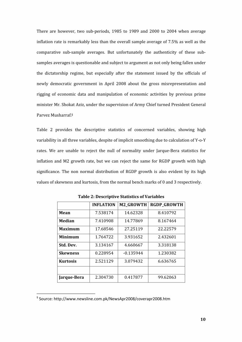
Table 2 provides the descriptive statistics of concerned variables, showing high
variability in all three variables, despite of implicit smoothing due to calculation of Y-o-Y
rates. We are unable to reject the null of normality under Jarque-Bera statistics for
inflation and M2 growth rate, but we can reject the same for RGDP growth with high
significance. The non normal distribution of RGDP growth is also evident by its high
values of skewness and kurtosis, from the normal bench marks of 0 and 3 respectively.
Table 2: Descriptive Statistics of Variables
INFLATION M2_GROWTH RGDP_GROWTH
Mean 7.538174 14.62328 8.410792
Median 7.410908 14.77869 8.167464
Maximum 17.68546 27.25119 22.22579
Minimum 1.764722 3.931652 2.432601
Std. Dev. 3.134167 4.660667 3.318138
Skewness 0.228954 -0.135944 1.230382
Kurtosis 2.521129 3.079432 6.636765
Jarque-Bera 2.304730 0.417877 99.62063
§ Source: http://www.newsline.com.pk/NewsApr2008/coverapr2008.htm

11
Probability 0.315889 0.811445 0.000000
Observations 126 125 124
2.3 Stationarity of Variables and Preliminary Cointegration Analysis
To check the order of integration in considered time series, we conduct the unit root
tests in this section. Augmented Dickey-Fuller (ADF) and Phillips-Perron(PP) tests were
used and the results (Table 3) shows that Inflation is seriously affected by the problem
of unit root and thus Non stationary. On the other hand, for M2 Growth, we have strong
evidences to reject the presence of unit root forcing us to believe on its stationary
behavior. The values of Durbon Watson statistic also strengthen our conclusion about
stationarity of M2 Growth. However the results for Real GDP growth are somewhat
persuasive rather than conclusive. ADF tests clearly reject the possibility of its
stationarity showing strong presence of unit root. But on the other hand Philliip Perron
tests reject the null of unit root at 10% and 5% but this rejection is itself questionable
due to low values of Durbon Watson statistics pointing out us towards the possible
deterioration of results due to serial correlation. Interestingly if we rely on
Kwiatkowski-Phillips-Schmidt-Shin (KPSS) test to check the stationarity of Inflation, M2
Growth and Real GDP growth, we won’t be able to have enough evidences to reject the
null hypotheses of stationarity for all variables (results not reported) which is
contradictory to the results of ADF and PP test for Inflation and Real GDP growth.
Table 3: Unit root testing
INFLATION Statistic Prob Lags/BW AIC SIC DW Stats
ADF (constant term) -1.519847 0.5203 4(SIC) 3.402107 3.540742 1.791038
ADF (constant, trend) -1.370435 0.8648 4(SIC) 3.414736 3.576476 1.798311
PHILLIP PERRON (constant term) -2.200326 0.2073 6 3.600122 3.645375 1.338362
PHILLIP PERRON (constant, trend) -1.918631 0.6389 7 3.605208 3.673088 1.362273
MONEY GROWTH Statistic Prob Lags/BW AIC SIC DW Stats

12
ADF (constant term) -3.560129 0.0080 4(SIC) 4.471723 4.611098 2.014176
ADF (constant, trend) -3.546606 0.0390 4(SIC) 4.487793 4.650396 2.013185
PHILLIP PERRON (constant term) -3.344702 0.0149 1 4.621648 4.667137 2.006133
PHILLIP PERRON (constant, trend) -3.290910 0.0726 1 4.637686 4.705918 2.007551
RGDP GROWTH Statistic Prob Lags/BW AIC SIC DW Stats
ADF (constant term) -2.461377 0.1276 6(SIC) 2.372044 2.560910 1.943435
ADF (constant, trend) -2.477490 0.3387 6(SIC) 2.387854 2.600329 1.943356
PHILLIP PERRON (constant term) -3.301906 0.0169 6 3.621104 3.666831 0.657080
PHILLIP PERRON (constant, trend) -3.299109 0.0712 6 3.636733 3.705323 0.657271
Note:***,**,* respectively indicates rejection of the null at 1%, 5% and 10% significance levels.
The above mentioned results prompt us to conduct Cointegration test, under the
assumption of I(1) covariance stationarity of all variables, to estimate any long run
relationship among them, if it exist.
Table 4: Johansen Cointegration Test for �, ��� � !�
No. of
Cointegrating
Vectors under
the Null
Hypothesis
Trace Test Maximum Eigenvalue Test
"����
5%
Critical
Value
Prob. "��#
5%
Critical
Value
Prob.
None 44.54070 35.19275 0.0037 22.66782 22.29962 0.0444
At most 1 21.87288 20.26184 0.0298 18.03823 15.89210 0.0227
At most 2 3.834646 9.164546 0.4373 3.834646 9.164546 0.4373
The Johansen test statistics (Table 4) show rejection for the null hypothesis of no
cointegrating vectors under both the trace and maximal eigenvalue forms of the test.
Moving on to test the null of at most 1 cointegrating vectors, the trace statistics is 21.87,
while the 5% critical value is 20.26, so the null is just rejected at 5% (and not rejected at
1%). Finally examining the null that there are at most 2 cointegrating vectors, the trace
statistic is now well below the 5% critical value, suggesting that the null should not be
rejected, i.e. there are at most two cointegrating vectors. $1 & ' & 2)

13
We also applied Engle-Granger(EG) approach to test the cointegrating relationship
among variables, according to which equilibrium errors of cointegrating regression
must be stationary for the variables to be cointegrated in long run.
�� � " * +���� * ,!�� * -� Equation 1
Estimated long run coefficients of .2/0 and 1/0calculated from equation 1 are reported
in table 5.
Table 5: Regression Results of Equation 1
Variables Coefficients
Constant 2.116196**
M2 growth rate (.2/) 0.167641***
Real GDP growth rate (1/) 0.339489***
Adjusted R-Square 0.183155
D-W stat 0.286444
Akaike info criterion 4.855724
Schwartz info criterion 4.923956
F-statistics 14.78970***
Note:***,**,* respectively indicates rejection of the null at 1%, 5% and 10% significance levels.
Unit root tests of 20, obtained from equation 1, are given in Table 6 indicating that
residuals of cointegrating regression are I(0) according to ADF and PP test at 10% and
5% respectively. However we cannot reject the presence of unit root in the residuals of
cointegrating regression if we introduce trend term.
Table 6: Unit Root Test for residuals of cointegrating
regression
Statistic
ADF (constant) -2.605347*
ADF (constant, trend) -2.710422
PHILLIP PERRON (constant) -3.027887**
PHILLIP PERRON (constant, trend) -3.023582
Note:***,**,* respectively indicates rejection of the null at 1%, 5% and 10% significance levels.

14
3. Inflation Uncertainty Framework
In this section we discussed ARCH model and its extensions such as GARCH, Asymmetric
GARCH (AGARCH), Threshold GARCH (TGARCH) and Exponential GARCH (EGARCH) to
analyze the relationship between Inflation and Inflation Uncertainty. The formal
presentation of ARCH(q) model given by Engel (1982) is
��|4��5~ 7$89��5, �) Equation 2
:��5-�� � � � ;� * ∑ ;�-����=�>5 Equation 3
Where equation 2 represents conditional mean of Inflation at time t which depends
upon the information set at time period t-1 $?0�@) . Equation 3 is conditional variance of
unanticipated shocks to inflation which is equal to 20 � A0 � BC0�@ and is actually
expected value of conditional variance at time t-1, conditioned upon the information set
available at time t-1.
If D@ � DE � DF � DG � 0 then conditional variance of errors is constant, however to
allow conditional variance as time varying measure of inflation uncertainty (presence of
ARCH) at least one of the DI J 0 KLM'M $N � 1,2, … … . , Q). By applying the restriction
∑ DIGI>@ R 1 we ensure that ARCH process is covariance stationary. Non negativity of all
ARCH parameters DIis sufficient but not necessary condition to ensure that conditional
variance doesn’t become negative.
However, evidence of long lag processes of Squared residuals in ARCH model suggested
that shocks have persistence affects on inflation uncertainty, thus Bollerslev (1986) and
Taylor (1986) independently suggested alternative GARCH approach for modeling
persistence, according to which the linear GARCH(p,q) process in Equation 4 represents
the conditional variance of inflation forecast error which is a function of lagged values
of both one period forecast error and the conditional variance.

15
� � ;� * ∑ ;�-����=�>5 * ∑ ST��T�T>5 Equation 4
Where ;� U 0, ;� J V � � � 5, �, … … . , =
ST J V � T � 5, �, … … . , �
GARCH is more parsimonious compared to ARCH as with only three parameters it
allows an infinite number of past squared errors to influence the current conditional
variance, Chris Brooks (2002), and is less likely to breach non-negativity constraints, but
the primary restriction of GARCH is that it enforce a symmetric response of volatility to
positive and negative shocks. According to Brunner and Hess (1993) and Joyce (1995), a
positive inflation shock is more likely to increase Inflation uncertainty via monetary
policy mechanism, as compared to negative inflation shock of equal size. If it is true then
we cannot rely on the estimates of symmetric ARCH and GARCH models and will have to
go for asymmetric GARCH models. Two popular asymmetric formulations are GJR
model, named after the authors Glosten, Jagannathan and Runkle (1993) and the
exponential GARCH (EGARCH) model proposed by Nelson (1991).
GJR-GARCH is simply an extension of GARCH(p,q) with an additional term to capture the
possible asymmetries (leverage effects). The conditional variance is now
� � ;� * ;5-��5� * S5��5 * W-��5� X��5 Equation 5
Where Y0�@= 1, if 20�@ < 0, otherwise Y0�@= 0. If the asymmetry parameter Z is negative
then negative inflationary shocks result in the reduction of inflation uncertainty.
(Bordes et al. 2007)
The exponential GARCH model was proposed by Nelson (1991). There are various ways
to express the conditional variance equation, but one possible specification is
��[� � ;� * ∑ ST=T>5 ��[��T * ∑ ;���>5 \ -�]�^�]�\ * ∑ W_�_>5 -�]_^�]_ Equation 6

16
EGARCH model has several advantages over the traditional ARCH and GARCH
specifications. First, variance specification represented in equation 6 makes it able to
capture the asymmetric effects of good news and bad news on volatility, which is
preferable in the context of Inflation and Inflation uncertainty. Second, since the `abL0
is modeled, then even in the presence of negative parameters, L0will be positive thus
relieving the non-negativity constraints artificially imposed on GARCH parameters.
4. Estimation and Results
4.1 Construction of Mean Equation
Though the initial unit root tests and cointegration analysis show that A0, .2/0 and
1/0are stationary and they might be cointegrated in the long run, still the results are not
highly significant and we have equal reasons (rejection of null of unit root at 10%
significance level) to formulate a model in the original form of variables instead of their
detrended series. We choose to model inflation in autoregressive distributed lag (ADL)
form:
c$d)�� � " * +$d)���� * ,$d)!�� * -� Equation 7
Where e$f), g$f), and h$f) are appropriate lag polynomials of A0, .2/0, and
1/0respectively. There are strong evidences that Inflation in Pakistan is a monetary
phenomenon, Qayyum (2006), Kemal(2006) strongly suggested that excess money
supply growth has been a significant contributor to the rise in inflation in Pakistan.
Khalid (2005) used Bivariate VAR analysis to conclude that seigniorage and money
depth may be considered among the major determinants of Inflation in Pakistan. Ahmad
et al(1991) found that major determinants of Inflation among others are, lagged
inflation and nominal money growth. In an IMF working paper, Axel Schimmelpfennig et
al(2005) developed three different models to forecast inflation, Univariate model
(ARIMA based), Unrestricted VAR model and Leading Indicators Model (LIM), and they

17
found LIM based on broad money growth, private sector credit growth and lags in
Inflation, best for ex-post inflation forecast in Pakistan. A0 and .2/0has correlation of
0.23 which increases to 0.29, 0.34 and 0.36 if we take .2/0�@, .2/0�Eand .2/0�F
instead of .2/0, which clearly indicates the transmission delay in monetary stance, thus
making us more confident about the selection of ADL model. In this scenario we expect
gi to be positive and significant.
The bidirectional relationship between Inflation and growth is widely accepted,
however according to classical Quantity theory of money, under the assumption of
constant velocity and M2 growth, real GDP growth should have a negative impact on
Inflation. Domac and Elbrit (1998) did cointegration analysis and developed ECM for
Albanian data and found evidence in support of classical supply shocks theory that
growth, through structural reforms and improved infrastructure, can significantly
reduce inflation. Handerson (1999), Becker and Gordon (2005), Murphy (2007), Robert
McTeer (2007) are among many, who strongly believe that increasing growth have
strong impacts of inflation in an opposite direction. Recently in 2008, ECB’s and
Bundesbank presidents said that “Slowing growth may not be sufficient to reduce
inflation in Eurozone” thus negating as well the positive relationship between inflation
and growth therefore despite of obtaining strong positive and significant relationship
found between A0 and 1/0 from cointegrating regression (equation 1), we still expect
negative sign of hi in our model explaining the negative impact of supply shocks on
inflation, especially with lagged values of 1/0.
The reason for the inclusion of autoregressive term e$f)A0is straight forward. Inflation,
like many other economic variables, has shown strong inertia in various studies. There
may be many reasons for this inertia like inability of market agent to interpret and
respond timely after an arrival of a particular announcement or news, or the probability
of uncertainty attached with that news or the overreaction of market participants by

18
following the herd behavior. In case of presence of strong inflationary inertia, as it is
evident from many studies, we expect ei to be positive and highly significant.
The optimal number of lags is obtained by using Akaike and Schwartz information
criteria (AIC) and (BIC) and in that case it is one, both for autoregressive term and
distributed lag term, so we finalized ADL(1, 1) model to estimate mean inflation.
�� � " * c5���5 * +5�����5 * ,5!���5 * -� Equation 8
Regression results of equation 8 are reported in table 7:
Table 7: Regression results of ADL(1,1)
model
Variables Coefficients
j 0.335366
e@ 0.897731***
g@ 0.058195**
h@ -0.049717
Adjusted R-Square
0.810313
AIC = 3.410951,
BIC = 3.501928
F-Statistic
176.1451***
DW-Stat
1.5883
Breusch-Godfrey Serial
Correlation LM Test:
Lag 4 = 20.1297***
ARCH LM Test:
Lag 4 = 6.2354
Note:***,**,* respectively indicates rejection of the null at 1%, 5% and 10% significance levels.
Due to presence of significant serial correlation in residuals of above model as indicated
by Breusch-Godfrey test and Ljung-Box Q statistics, we introduced AR(1) and AR(4)
error term in equation 7. Lag orders of error term identified through partial
autocorrelogram function (PAF) of residuals. So the model becomes:
�� � " * c5���5 * +5�����5 * ,5!���5 * ��
�� � k5���5 * k����� * -� Equation 9

19
Table 8: Results of equation 9
Variables Coefficients
j 0.130386
e@ 0.929164***
g@ 0.051121**
h@ -0.037501
l@ 0.168262*
lm -0.373843***
Adjusted R-Square
0.850537
AIC=3.203545,
BIC=3.342919
F-Statistic
136.43681***
DW-Stat
1.914897
Breusch-Godfrey Serial
Correlation LM Test:
Lag 4=5.75716
ARCH LM Test:
Lag 4=5.14009
Note:***,**,* respectively indicates rejection of the null at 1%, 5% and 10% significance levels.
After introducing AR specification of residuals, we found no evidence of serial
correlation in DW Stat, Breusch-Godfrey test and Ljung Box Q-Statistics (reported in
table 9). R-Square also improved by about 4% due to inclusion of autoregressive
components of errors.
Table 9: Q-Stat table for Residuals
Lag Q-Stat Prob.
3 0.7523 0.386
5 2.1809 0.536
10 5.1320 0.743
15 14.800 0.320
20 19.225 0.378
25 20.991 0.582
30 22.747 0.746
35 25.970 0.803
4.2 Estimation of Uncertainty

20
As far as variance equation is concerned, we didn’t find any ARCH model from ARCH(1)
to ARCH(4) with significant estimated parameters along with conformity of constraints
imposed on ARCH(p) process, so we decided to go for GARCH estimation. Table 10
provides the results of 2 different models.
Table 10: GARCH estimations of
conditional variance
Model 1 Model 2
Mean Equation
Variables GARCH(1,1) GARCH(1,1)
" 0.147506 -0.235069
c5 0.937117*** 0.936293***
+5 0.045557* 0.047618**
,5 -0.031433
k5 0.175788 0.201809*
k� -0.411784*** -0.419355***
Variance Equation
;� 1.645441*** 0.207634
;5 0.235475* 0.315353***
S5 -0.438056 0.608708***
W
R-Square 0.845660 0.831154
DW Stat 1.926282 1.685223
Akaike
criterion 3.214446 3.316416
Schwarz
criterion 3.423507 3.501262
F-Stat 82.50290*** 85.38659***
Note:***,**,* respectively indicates rejection of the null at 1%, 5% and 10% significance levels.
4.3 Tests for Asymmetries in Volatility:
Engle and Ng (1993) have devised a set of tests to confirm the asymmetry present in
volatility, if any. These tests are generally known as Sign and Size bias tests. We used

21
these tests to determine whether an asymmetric model is required to capture the
inflation uncertainty or whether the GARCH model can be an adequate model.
We applied sign and size bias tests on the residuals of GARCH(1, 1) (Model 02) whose
mean and variance equations are given below
Mean Equation:
�� � " * c5���5 * +5�����5 * ��
�� � k5���5 * k����� * -�
Variance Equation:
� � ;� * n ;�-����=
�>5* n ST��T
�
T>5
Where ;� U 0, ;� J V � � � 5, �, … … . , =
ST J V � T � 5, �, … … . , �
The test for sign bias is based on the significance or otherwise of o@ in equation 10.
-p�� � q� * q5r��5� * s� Equation 10
r��5� �� 5 �� -��5 R 0 tuv 0 awLM'KNiM
Where x0is an iid error term. If the impact of positive and negative inflation shocks is
different on conditional variance, then o@will be statistically significant.
It is most likely, especially in case of inflation that the magnitude or size of the inflation
shock will affect whether the response of volatility to shock is symmetric or not. Engle
and Ng originally suggested a negative sign bias test, based on a regression where r��5�
is now used as a slope dummy variable. Negative sign bias is argued to be present if o@ is
statistically significant in the euqtion 11.

22
-p�� � q� * q5r��5� -��5 * s� Equation 11
However we made little change in that and conducted the above test as positive sign
bias test additionally.
-p�� � q� * q5r��5y -��5 * s� Equation 12
r��5z �� 5 �� -��5 U 0 tuv 0 awLM'KNiM
Finally Setting {0�@y � 1 � {0�@� so that {0�@y would become the dummy to capture
positive inflation shocks, Engle and Ng (1993) proposed a joint test for size and sign bias
based on following regression;
-p�� � q� * q5r��5� * q�r��5� -��5 * q|r��5y -��5 * s� Equation 13
Significant value of o@ in equation 13 indicates the presence of sign bias i.e. positive and
negative inflation shocks have different impacts upon future uncertainty. On the other
hand, the significant values of oE and oF would suggest the presence of size bias, where
the sign and the magnitude of shock, both are important. A joint test statistics is }1E
which will asymptotically follow a ~E distribution with 3 degrees of freedom under the
null hypothesis of no asymmetric effects.
Table 11: Tests for Asymmetries in Volatility
Sign Bias Test
Eq. 10
Negative Sign
Bias Test
Eq. 11
Positive Sign
Bias Test
Eq. 12
Joint test for
Sign and Size
Bias
Eq. 13
o� 1.901442*** 1.681014*** 1.001339*** 0.481507
o@ -0.661602 0.224811 1.230697*** 0.557517
oE -0.228534
oF 1.566024***
}1E 8.92332**

23
The individual regression results of Sign bias test and negative sign bias test doesn’t
reveal any evidence of asymmetry as the value of o@is insignificant. But we can see that
the coefficient indicating the positive sign bias is significant in individual as well as in
joint test. In addition, although none of the other coefficients except oF are significant in
the joint regression, the ~E test statistic is significant at 5%, suggesting a rejection of the
null hypothesis of no asymmetries.
The above results lead us to go for asymmetric GARCH models instead of symmetric and
in table 12 we report the results of 3 asymmetric GARCH models.
Table 12: GJR-GARCH and EGARCH estimations of
conditional variance
Model 3 Model 4 Model 5
Variables GJR-GARCH GJR-GARCH EGARCH
" -0.024369 -0.236679 0.065636
c5 0.913173*** 0.914421*** 0.917033***
+5 0.064182** 0.062802 0.053746***
,5 -0.030109 -0.036433*
k5 0.203838** 0.188266 0.160722***
k� -0.424543*** -0.339855** -0.401705***
;� 0.414841* 1.436776 0.220033
;5 0.071345 0.077708 0.265016***
S5 0.671568*** 0.477734 -0.954307***
W -0.151450 -0.293339** 0.139627**
R-Square 0.843248 0.829570 0.842640
DW Stat 1.932040 1.648933 1.844275
Akaike
criterion 3.218947 3.490593 3.160134
Schwarz
criterion 3.452486 3.699655 3.392425
F-Stat 71.53131*** 73.40415*** 71.80327***
Note:***,**,* respectively indicates rejection of the null at 1%, 5% and 10% significance levels.

24
Results from GJR-GARH (Model 3 and 4) confirmed that these models are successful in
modeling asymmetric (leverage effects) of lagged inflation shocks on one period ahead
conditional variance. From both models we obtained the negative values of W as
expected, thus concluding that negative inflation shocks (good news) reduce inflation
uncertainty. On the other hand the value of W is positive and significant in EGARCH
estimation (Model 5) suggesting that when there is an unexpected increase in inflation,
resulting positive inflation shocks (bad news), inflation uncertainty increases more than
when there is a unanticipated decrease in inflation.
4.4 News Impact Curves
For further investigation of asymmetric behavior of inflation uncertainty, we analyzed
the effects of news on volatility or inflation uncertainty with the help of “News Impact
Curve”. By keeping constant all the information at t-2 and earlier, we can examine the
implied relation between 20�@ and L0 which we called as “News Impact Curve”. It is a
pictorial representation of the degree of asymmetry of volatility to positive and negative
shocks and it plots next period uncertainty L0 that would arise from various positive and
negative values (news) of past inflation shocks (20�@) [Pagan and Schwert, 1990]. For
the GARCH model, this curve is a quadratic function centered at 20�@ � 0. The equations
of News impact curve for the GARCH, GJR-GARCH and EGARCH models are provided in
table 13.
Table 13: News Impact Curve for different GARCH processes
GARCH(1,1)
L0 � � * D@20�@E
Where � � D� * �@��E
And ��E � D�/�1 � D@ � �@�
GJR-GARCH(1,1)
Or
TGARCH(1,1)
L0 � � * $D@ * Z@Y0�@)20�@E
Where � � D� * �@��E
And ��E � D�/�1 � D@ � �@ � ���E ��

25
EGARCH(1,1)
L0 � � exp �D@$|20�@| * Z@20�@)�� �
Where � � ��E��exp �D��
��E � exp �D� * D@^2 A⁄1 � �@ �
Source: Eric Zevot (2008), “Practical Issues in the Analysis of Univariate GARCH Models”
Where L0is the conditional variance at time t, 20�@is inflation shock at time t-1, �� is the
unconditional standard deviation of inflation shocks, D� and �@ are constant term and
parameter corresponding to L0�@in GARCH variance equation respectively.
The resulting news impact curves for GARCH, GJR-GARCH and EGARCH models are given
in figure 5.
Figure 5(a) Figure 5(b)
It can be seen in figure 5(a) and 5(b), that GARCH news impact curves are of course
symmetrical about zero, so that a shock of given magnitude will have the same impact
on the future volatility, irrespective of its sign. On the other hand GJR news impact
curves [figure 5(c) and 5(d)] are asymmetric where negative inflation shocks are in fact
reducing the future volatility exactly as it was aimed to model through equation 5.
1
2
3
4
5
-4 -3 -2 -1 0 1 2 3 4
RES_MODEL02(-1)
HT_MODEL02
1.0
1.5
2.0
2.5
3.0
3.5
4.0
-4 -3 -2 -1 0 1 2 3 4
RES_MODEL01(-1)
HT_MODEL01

26
Figure 5(c) Figure 5(d)
Figure 5(e)
Figure 5(e) is also according to our expectation where we see that unexpected increase
in inflation (positive inflation shocks) increases volatility more than when there is a
decrease in inflation that is what we can also interpret from the positive and significant
value of W reported for EGARCH model in table 12.
4.4 Testing of Friedman-Ball Hypothesis (Granger causality)
In order to assess Friedman-Ball and Cukierman-Meltzer hypotheses, we implement
Bivariate Granger-Causality test up to 10 lags, between inflation and inflation
0.5
0.6
0.7
0.8
0.9
1.0
1.1
1.2
1.3
-4 -3 -2 -1 0 1 2 3 4
RES_EG(-1)
XHT
-0.8
-0.4
0.0
0.4
0.8
1.2
-4 -3 -2 -1 0 1 2 3 4
RES_GJR01(-1)
HT_GJR01
0.0
0.4
0.8
1.2
1.6
2.0
2.4
2.8
3.2
3.6
-4 -3 -2 -1 0 1 2 3 4
RES_GJR02(-1)
HT_GJR02

27
uncertainty(one period ahead conditional forecast of variance), derived from model 1 to
model 5. The results for GARCH models (model 1 and 2) are reported in table 14(a). We
report only p-values of Wald statistics for the null hypothesis that “Inflation does not
cause Uncertainty” in the first column and that “Uncertainty does not cause Inflation” in
the second column for each model. The results reported in table 14(a) are not very
encouraging and they refused almost both Friedman-Ball and Cukierman-Meltzer
hypotheses, and it appears that neither of inflation or inflation uncertainty causes each
other.
Table 14(a): Granger Causality test (P-values of Wald Statistics)
Lags
GARCH (Model 01) GARCH (Model 02)
A vaMi uaw �t�iM L0
L0 vaMi uaw
�t�iM A A vaMi uaw
�t�iM L0
L0 vaMi uaw
�t�iM A 1 0.26888 0.72597 0.08924 0.62038
2 0.56460 0.25638 0.07732 0.72482
3 0.73427 0.38953 0.18948 0.51783
4 0.64214 0.46390 0.09205 0.29570
5 0.91466 0.30105 0.17072 0.12520
6 0.95092 0.12722 0.29456 0.10380
7 0.48360 0.18771 0.42834 0.21033
8 0.61851 0.37005 0.45173 0.18022
9 0.42338 0.53233 0.31722 0.21285
10 0.43627 0.31679 0.37353 0.21144
However results which we report in table 14(b) for GJR-GARCH (model 3 and 4) and
EGARCH (model 5), are consistent and strongly reject the null of “Inflation doest not
cause uncertainty” thus supporting Friedman-Ball hypothesis.

28
Table 14(b): Granger Causality test (P-values of Wald Statistics)
Lags
GJR-GARCH (Model 03) GJR-GARCH (Model 04) EGARCH (Model 05)
A vaMi uaw �t�iM L0
L0 vaMi uaw
�t�iM A A vaMi uaw
�t�iM L0
L0 vaMi uaw
�t�iM A A vaMi uaw
�t�iM L0
L0 vaMi uaw
�t�iM A 1 2.6E-05 0.41844 0.00446 0.63392 0.00058 0.07367
2 2.2E-25 0.84589 3.0E-17 0.54390 9.9E-08 0.02533
3 4.3E-27 0.84114 7.4E-20 0.17518 1.5E-08 0.07124
4 1.3E-27 0.00128 9.4E-24 0.08609 1.2E-08 0.00387
5 6.7E-33 0.94750 1.2E-25 0.99978 4.9E-08 0.27712
6 1.5E-35 0.39302 4.7E-26 0.85809 2.1E-09 0.52711
7 1.4E-33 0.08357 2.5E-25 0.69109 7.5E-08 0.17706
8 1.7E-32 0.18487 1.2E-23 0.08138 1.4E-07 0.21410
9 1.4E-30 0.02934 1.3E-22 0.16555 3.7E-06 0.45088
10 9.3E-32 0.11950 1.6E-23 0.33863 1.3E-05 0.45551
5. Conclusion
This study provides several interesting results. First of all we estimated inflation
uncertainty as time varying conditional variance of inflation shocks and found
performance of asymmetric GARCH models (GJR-GARCH and EGARCH) better than
simple GARCH models. GJR-GARCH estimates negative and significant value of “leverage
effect” parameter which suggests that negative shocks of inflation tends to decrease next
period uncertainty, this conclusion is also supported by the results of EGARCH models..
News Impact curves graphically reflect the asymmetric behavior of inflation uncertainty
from GJR-GARCH and EGARCH models. Finally bivariate Granger-Causality test strongly
support Friedman-Ball hypothesis for GJR-GARCH and EGARCH models, i.e. high
inflation causes inflation uncertainty and that the causality is running from inflation to
inflation uncertainty. We do not find any evidence in support of Cukierman-Meltzer
hypotheses.

29
References
Andersen, T.G., Bollerslev, T. (2006), "Volatility and Correlation Forecasting", Handbook
of Economic Forecasting, Vol. 1.
Apergis, N. (2006), “Inflation, output growth, volatility and causality: evidence from
panel data and G7 countries”, Economics Letters, 83 (2004) 185-191.
Ball, L. (1992), “How does inflation raise inflation uncertainty?”, Journal of Monetary
Economics, 29, 371‐388.
Berument, H. et al (2001), “Modeling Inflation Uncertainty Using EGARCH: An
Application to Turkey”, Bilkent University Discussion Paper.
Bilquees, F. (1988), “Inflation in Pakistan: Empirical Evidence on the Monetarist and
Structuralist Hypotheses”, The Pakistan Development Review 27:2, 109–130.
Bollerslev, T. (1986), “Generalized Autoregressive Conditional Heteroscedasticity”,
Journal of Econometrics, 31, 307‐27.
Bollerslev, T., and J.M. Wooldridge, (1992), “Quasi-Maximum Likelihood Estimation and
Inference in Dynamic Models with Time-Varying Covariances”, Econometric Reviews, 11,
143-172.
Bokil, M. and Schimmelpfennig, A. (2005), “Three Attempts at Inflation Forecasting in
Pakistan”, IMF Working Paper, WP/05/105.
Bordes, C. et al (2007), “Money and Uncertainty in the Philippines: A Friedmanite
perspective”, Conference paper, Asia-Link Program.
Bordes, C. and Maveyraud, S. (2008), “The Friedman’s and Mishkin’s Hypotheses
(re)considered”, Unpublished.
Brunner, A.D. and Hess, G.D. (1993), “Are Higher Levels of Inflation Less Predictable? A
State-Dependent Conditional Heteroscedasticity Approach”, Journal of Business &
Economic Statistics, Vol. 11, No. 2, (Apr., 1993), pp. 187-197.
Brunner, A.D. and Simon, D.P. (1996), “Excess Returns and Risk at the long End of The
Treasury Market: an EGARCH-M Approach”, The Journal of Financial Research, 14, 1, 443-
457.
Caporale, T and McKiernan, B. (1997), “High and Variable Inflation: Further Evidence on
the Friedman Hypothesis”, Economic Letters 54, 65-68.
Chaudhary, M. Aslam, and Naved Ahmad, (1996), “Sources and Impacts of Inflation in
Pakistan,” Pakistan Economic and Social Review, Vol. 34, No. 1, pp. 21–39.
Cosimano, T. and Dennis, J. (1988), “Estimation of the Variance of US Inflation Based
upon the ARCH Model”, Journal of Money, Credit, and Banking, 20(3) 409-423.
Crowford, A. and Kasumovich, M. (1996), “Does Inflation Uncertainty vary with the Level
of Inflation?”, Bank of Canada, Ottawa Ontario Canada K1A 0G9.

30
Engle, R. (1982), “Autoregressive Conditional Heteroscedasticity with Estimates of
United Kingdom Inflation”, Econometrica, 987-1007.
Fountas, S. et al (2000), “A GARCH model of Inflation and Inflation Uncertainty with
Simultaneous Feedback”.
Fountas, S. et al (2006), “Inflation Uncertainty, Output Growth Uncertainty and
Macroeconomic Performance”, Oxford Bulletin of Economics and Statistics, 68, 3 (2006)
0305-9049.
Franses, P.H. (1990), “Testing For Seasonal Unit Roots in Monthly Data”, Econometric
Institute Report, No.9032A, Erasmus University, Rotterdam.
Friedman, M. (1977), “Nobel Lecture: Inflation and Unemployment”, Journal of Political
Economy, Vol. 85, 451-472.
Glosten, L. R., R. Jagannathan and D. Runkle, (1993), “On the Relations between the
Expected Value and the Volatility of the Normal Excess Return on Stocks”, Journal of
Finance, 48, 1779‐1801.
Golob, John E. (1994), “Does inflation uncertainty increase with inflation?”, Federal
Reserve Bank of Kansas City - Economic Review. Third Quarter 1994.
Grier,K., Perry, M. (2000), “The effects of real and nominal uncertainty on inflation and
output growth: some GARCH-M evidence”, Journal of Applied Econometric 15, 45-48.
Holland, A. S. (1984), “Does Higher Inflation Lead to More Uncertain Inflation?”, Federal
Reserve Bank of St. Louis Review 66, 15-26.
Hafer, R. W. (1985), “Inflation Uncertainty and a test of the Friedman Hypothesis”,
Federal Reserve Bank of St. Louis Working Paper 1985-006A.
Hu, M.Y., C.X. Jiang, and C. Tsoukalas, (1997), “The European Exchange Rates Before and
After the Establishment of the European Monetary System”, Journal of International
Financial Markets, Institutions and Money, 7, 235- 253.
Khalid, A. M. (2005), “Economic Growth, Inflation and Monetary Policy in Pakistan:
Preliminary Empirical Estimates”, The Pakistan Development Review,44 : 4 Part II
(Winter 2005) pp. 961–974.
Khan, M. S., and S. A. Senhadji (2001), “Threshold Effects in the Relationship between
Inflation and Growth”, IMF Staff Papers 48:1.
Khan, A. H., and M. A. Qasim (1996)’ “Inflation in Pakistan Revisited”, The Pakistan
Development Review 35:4, 747–759.
Khan, M. S., and A. Schimmelpfennig (2006), “Inflation in Pakistan: Money or Wheat?”,
IMF Working Paper, wp/06/60.
Koutmos, G., and G.G. Booth, (1995), “Asymmetric Volatility Transmission in
International Stock Markets”, Journal of International Money and Finance, 14, 747-762.
Malik, W. Shahid and Ahmad, A. Maqsood (2007), “The Taylor Rule and the
Macroeconomic performance in Pakistan”, The Pakistan Development Review, 2007:34.

31
Malik, W. Shahid (2006), “Money, Output and Inflation: Evidence from Pakistan”, The
Pakistan Development Review 46:4.
Nas, T. F. and M.J. Perry, (2000), “Inflation, Inflation Uncertainty and Monetary Policy in
Turkey”, Contemporary Economic Policy, 18, 170-180.
Nelson, D.B. (1991), “Conditional Heteroscedasticity in Asset Returns: A New Approach”,
Econometrica, 59, 347-370.
Price, Simon, and Anjum Nasim, (1999), “Modeling Inflation and the Demand for Money
in Pakistan: Cointegration and the Causal Structure,” Economic Modeling, Vol. 16, pp. 87–
103.
Thornton, J. (2006), “High and variable inflation: further evidence on the Fried- man
hypothesis”, Southern African Journal of Economics, 74, 167-71.
Tse, Y., and G.G. Booth, (1996), “Common Volatility and Volatility Spillovers Between U.S.
and Eurodollar Interest Rates: Evidence from The Features Market”, Journal of
Economics and Business, 48, 299-312
Qayyum, A. (2006), “Money, Inflation and Growth in Pakistan”, The Pakistan
Development Review 45 : 2 (Summer 2006) pp. 203–212.
Zivot, E. (2008), “Practical Issues in the Analysis of Univariate GARCH Models”,
Unpublished.

32
Appendix
Figure 6: Forecast of Conditional Variance (Inflation Uncertainty)
0
1
2
3
4
1980 1985 1990 1995 2000 2005
VAR_GARCH01
0
1
2
3
4
5
6
1980 1985 1990 1995 2000 2005
VAR_GARCH02
0.0
0.5
1.0
1.5
2.0
2.5
3.0
1980 1985 1990 1995 2000 2005
VAR_GJR01
0.0
0.4
0.8
1.2
1.6
2.0
2.4
2.8
3.2
3.6
1980 1985 1990 1995 2000 2005
VAR_GJR02
0.4
0.8
1.2
1.6
2.0
2.4
2.8
3.2
3.6
4.0
1980 1985 1990 1995 2000 2005
VAR_EG

33

34
Figure 7: Impulse Response Functions of Uncertainty to Inflation
-.12
-.08
-.04
.00
.04
.08
.12
.16
1 2 3 4 5 6 7 8 9 10
Response of VAR_GARCH01 to INFLATION
-.1
.0
.1
.2
.3
1 2 3 4 5 6 7 8 9 10
Response of VAR_GARCH02 to INFLATION
-.10
-.05
.00
.05
.10
.15
.20
1 2 3 4 5 6 7 8 9 10
Response of VAR_GJR01 to INFLATION
-.2
-.1
.0
.1
.2
.3
.4
1 2 3 4 5 6 7 8 9 10
Response of VAR_GJR02 to INFLATION
-.2
-.1
.0
.1
.2
.3
1 2 3 4 5 6 7 8 9 10
Response of VAR_EG to INFLATION
Response to Cholesky One S.D. Innovations ± 2 S.E.


![Dua-e-Kumail - in Conceptual Style€¦ · DUA-E-KUMAIL - IN CONCEPTUAL STYLE [Document subtitle] ABSTRACT Dua-e-Kumail is now one of the most read supplications of Imam Ali (AS)](https://img.pdfslide.us/doc/110x75/605b21c8479bfc022b674715/dua-e-kumail-in-conceptual-style-dua-e-kumail-in-conceptual-style-document.jpg)