Astronomy c ESO 2006 Astrophysics - CORE · from La Palma (Spain) and SAAO (South Africa). However, due to poor weather conditions, the only useful data were those taken at La Palma

A&A 452, 987–1000 (2006)DOI: 10.1051/0004-6361:20053615c© ESO 2006

Astronomy&

Astrophysics

Analysis and modeling of high temporal resolution spectroscopicobservations of flares on AD Leonis

I. Crespo-Chacón1, D. Montes1, D. García-Alvarez2,3, M. J. Fernández-Figueroa1,J. López-Santiago1,4, and B. H. Foing5

1 Departamento de Astrofísica, Facultad de Ciencias Físicas, Universidad Complutense de Madrid, 28040 Madrid, Spaine-mail: [email protected]

2 Harvard-Smithsonian Center for Astrophysics, 60 Garden Street, Cambridge, MA 02138, USA3 Armagh Observatory, College Hill, Armagh BT61 9DG, Northern Ireland4 Osservatorio Astronomico di Palermo, Piazza del Parlamento 1, 90134 Palermo, Italy5 Research Division, ESA Space Science Department, ESTEC/SCI-R, PO Box 299, 2200 AG Noordwijk, The Netherlands

Received 10 June 2005 / Accepted 1 February 2006

ABSTRACT

We report the results of a high temporal resolution spectroscopic monitoring of the flare star AD Leo. During 4 nights, more than600 spectra were taken in the optical range using the Isaac Newton Telescope (INT) and the Intermediate Dispersion Spectrograph(IDS). We observed a large number of short and weak flares occurring very frequently (flare activity > 0.71 h−1). This is consistent withthe very important role that flares can play in stellar coronal heating. The detected flares are non white-light flares and, although mostsolar flares are of this kind, very few such events have been observed previously in stars. The behaviour of different chromosphericlines (Balmer series from Hα to H11, Ca iiH & K, Na iD1 and D2, He i 4026 Å and He iD3) was studied in detail for a total of 14 flares.We estimated the physical parameters of the flaring plasma by using a procedure that assumes a simplified slab model of flares. Allthe obtained physical parameters are consistent with previously derived values for stellar flares, and the areas – less than 2.3% ofthe stellar surface – are comparable with the size inferred for other solar and stellar flares. We studied the relationships between thephysical parameters and the area, duration, maximum flux and energy released during the detected flares.

Key words. stars: activity – stars: chromospheres – stars: flare – stars: late-type – stars: individual: AD Leo

1. Introduction

Stellar flares are events where a large amount of energy is re-leased in a short interval of time, with changes taking place atalmost all frequencies in the electromagnetic spectrum. Flaresare believed to be the result of the release of part of the magneticenergy stored in the corona through magnetic reconnection (seereviews by Mirzoyan 1984; Haisch et al. 1991; García-Alvarez2000). However, the exact mechanisms leading to the energy re-lease and subsequent excitation of various emission features re-main poorly understood. Many types of cool stars produce flares,sometimes at levels several orders of magnitude more energeticthan their solar counterparts (Pettersen 1989; García-Alvarezet al. 2002). In dMe stars (UV Ceti-type stars) optical flares are acommon phenomenon. On the contrary, in more luminous starsflares are usually only detected through UV or X-ray observa-tions (Doyle et al. 1989), although some optical flares have beenobserved in young early K dwarfs like LQ Hya and PW And(Montes et al. 1999; López-Santiago et al. 2003).

We would like to be able to trace all the energetic processesin a flare to a common origin, although the released energy canbe very different. The largest solar flares involve energies of1032 erg (Gershberg 1989). Large flares on dMe stars can betwo orders of magnitude larger (Doyle & Mathioudakis 1990;Byrne & McKay 1990), while very energetic flares are producedby RS CVn binary systems, where the total energy may exceed1038 erg (Doyle et al. 1992; Foing et al. 1994; García-Alvarezet al. 2003). Such a change in the star’s radiation field modi-fies drastically the atmospheric properties over large areas, fromphotospheric to coronal layers. Models by Houdebine (1992)

indicate that heating may be propagated down to low photo-spheric levels, with densities higher than 1016 cm−3. However,electrons with energies in the MeV range would be required toattain such depths.

Spectral emission lines are the most appropriate diagnos-tics to constrain the physical properties and motion of theflaring plasma (see Houdebine 2003, and references therein).Unfortunately, only a few sets of observations with adequatetime and spectral resolution are available so far (Rodonòet al. 1989; Hawley & Pettersen 1991; Houdebine 1992; Gunnet al. 1994b; García-Alvarez et al. 2002; Hawley et al. 2003).Furthermore, there are also few attempts to derive the physi-cal parameters of the flaring plasma (Donati-Falchi et al. 1985;Kunkel 1970; Gershberg 1974; Katsova 1990; Jevremovic et al.1998). García-Alvarez et al. (2002) obtained the first detailedtrace of physical parameters during a large optical flare, onAT Mic, using the Jevremovic et al. (1998) procedure. Goodquality spectroscopic observations, such as those analyzed in thiswork for AD Leo, and a correct description of the different flarecomponents are required to constrain numerical simulations.

AD Leo is well-known as a frequent source of flares. Ithas been the subject of numerous studies in the optical, EUVand X-ray because of its nature as one of the most activeM dwarfs (Pettersen et al. 1984, 1990; Lang & Willson 1986;Güdel et al. 1989; Hawley & Pettersen 1991; Hawley et al.1995, 2003; Abada-Simon et al. 1997; Cully et al. 1997; Favataet al. 2000; Sanz-Forcada & Micela 2002; van den Besselaaret al. 2003; Maggio et al. 2004; Robrade & Schmitt 2005;Smith et al. 2005). AD Leo (GJ 388) is classified as dM3Ve

Article published by EDP Sciences and available at http://www.edpsciences.org/aa or http://dx.doi.org/10.1051/0004-6361:20053615

http://www.edpsciences.org/aa

http://dx.doi.org/10.1051/0004-6361:20053615

988 I. Crespo-Chacón et al.: Analysis and modeling of flares on AD Leo

Table 1. Observing log INT/IDS (2–5 April 2001).

R1200B R1200YNight N UT texp(s) SNR N UT texp(s) SNR

start–end min–max min–max start–end min–max min–maxHβ Hγ Hδ Ca ii H H8 Hα Na i D1

Ca ii K H9 Na i D2

H10 He i D3

1 18 00:02–01:47 180–300 76–85 53–58 45–49 33–37 28–31 0 – – – –2 91 20:19–01:58 60–120 46–73 32–48 26–40 20–29 17–25 0 – – – –3 246 20:10–02:37 15–120 33–89 21–58 18–51 13–38 12–31 0 – – – –4 104 20:28–22:44 15–120 27–72 18–48 15–41 11–30 10–25 189 23:38–03:13 5–120 32–172 23–114

(Henry et al. 1994). This star has an unseen companion – de-tected using speckle interferometry – with a period of about27 years, which is expected to have a very low mass (Balegaet al. 1984). AD Leo is located in the immediate solar neigh-bourhood, at a distance of ∼4.9 pc (from the ground-based par-allax (Gray & Johanson 1991) – it was not a Hipparcos target).Its high activity is probably due to its high rotation rate (Pphot ∼2.7 days, Spiesman & Hawley 1986). Its rotational velocity(v sin i = 6.2 ± 0.8 km s−1) places AD Leo in the tail of rare fastrotating M dwarfs (Delfosse et al. 1998). The radius and massof AD Leo are R ∼ 0.44 R� and M ∼ 0.40 M� (Pettersen 1976;Favata et al. 2000). At this mass, stars are expected to have a sub-stantial radiative core, so that the interior structure is still “solar-like” (Chabrier & Baraffe 1997). Saar & Linsky (1985) de-tected, through infrared line measurements, photospheric fieldson AD Leo showing the presence of strong magnetic fields. Theyinferred that 73% of AD Leo’s surface is covered by active re-gions outside of dark spots containing a mean field strength ofB = 3800 ± 260 G.

Here we present the results of a long spectroscopic monitor-ing of AD Leo that was carried out using an intermediate dis-persion spectrograph and high temporal resolution. This workhas considerably extended the existing sample of stellar flaresanalyzed with good quality spectroscopy in the optical range.Details about the technical information of the observations anddata reduction are given in Sect. 2. Section 3 describes theanalysis of the observations and the detected flares, includingequivalent widths, line fluxes, released energy, line profiles andasymmetries. In Sect. 4 we present the main physical plasmaparameters obtained for the observed flares using the code de-veloped by Jevremovic et al. (1998). The discussion of the re-sults and conclusions are given in Sect. 5, where the relation-ships between the physical and observational parameters are alsoanalyzed. The preliminary results for this star and V1054 Ophwere presented by Montes et al. (2003) and Crespo-Chacón et al.(2004).

2. Observations and data reduction

The data were taken during the MUlti-SIte COntinuousSpectroscopy (MUSICOS) 2001 campaign. It involved obser-vations at two sites: El Roque de los Muchachos Observatoryfrom La Palma (Spain) and SAAO (South Africa). However,due to poor weather conditions, the only useful data were thosetaken at La Palma. This observing run was carried out with the2.5 m Isaac Newton Telescope (INT) from 2 to 5 April 2001.The Intermediate Dispersion Spectrograph (IDS) was utilizedtogether with the 2148 × 4200 EEV10a CCD detector. Twogratings were used: R1200B (every night) and R1200Y (sec-ond half of the last night). The wavelength covered by R1200B(blue spectrum) ranges from 3554 Å to 5176 Å (including the

Balmer lines from Hβ to H11 as well as the Ca ii H & K andHe i 4026 Å lines). The reciprocal dispersion of these spec-tra is 0.48 Å/pixel. The wavelength covered by R1200Y (redspectrum) ranges from 5527 Å to 7137 Å (including the Hα,Na i D1 & D2 and He i D3 lines) with a reciprocal dispersionof 0.47 Å/pixel. The spectral resolution, determined as the fullwidth at half maximum (FWHM) of the arc comparison lines, is1.22 Å for the blue region and 1.13 Å for the red one.

We took series of spectra with short exposure times: from 15to 300 s for R1200B and from 5 to 120 s for R1200Y. The spec-tra in each series were separated only by the CCD readout time(less than 60 s) in order to obtain the highest temporal resolu-tion possible. During 4 nights, a total of 459 spectra of AD Leowere obtained with R1200B and 189 with R1200Y. The observ-ing log (Table 1) lists the number of spectra taken each night (N),the universal time (UT) at the beginning and end of the AD Leoobservations, the minimum and maximum exposure time (texp)of the spectra, and the signal-to-noise ratio (SNR) of the contin-uum near each line region. These quantities are given for bothgratings (R1200B and R1200Y). Note that, despite the shortexposure times, the SNR is large enough to perform a reliableanalysis.

The reduction was done following the standard procedure:bias and dark subtraction, flat-field correction using exposuresof a tungsten lamp, cosmic rays correction, and sky backgroundsubtraction from the region of the aperture chosen for doing anoptimal extraction of each spectrum. The software packages ofIRAF1 were used. The wavelength calibration was done by usingspectra of Cu–Ar lamps. All the spectra were normalized to theirmaximum flux value of the observed continuum.

3. Analysis of the observations

In Fig. 1 we have plotted the observed blue spectrum of AD Leoin its quiescent state (minimum observed emission level) and atthe maximum of the strongest flare detected with the R1200Bgrating (flare 2, see Sect. 3.1). Figure 2 is similar to Fig. 1but for the red spectra, taken with the R1200Y grating, and thestrongest flare detected with this spectral configuration (flare 12,see Sect. 3.1). In addition, the spectra of Gl 687B and GJ 725Bhave been plotted as examples of inactive stars with a spec-tral type and luminosity class (M 3.5V) very similar to those ofAD Leo (M 3V). Note that the origin of the Y-axis is differentfor each spectrum in order to avoid overlap between them.

AD Leo shows a high level of chromospheric activity. Astrong emission in the Balmer series and the Ca ii H & K lines is

1 IRAF is distributed by the National Optical AstronomyObservatories, which are operated by the Association of Universitiesfor Research in Astronomy, Inc., under cooperative agreement with theNational Science Foundation.

I. Crespo-Chacón et al.: Analysis and modeling of flares on AD Leo 989

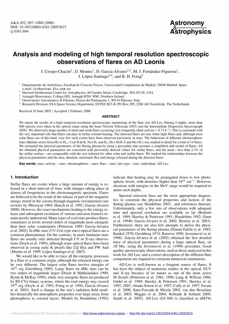
Fig. 1. Observed spectrum of AD Leo at the maximum of the strongest flare detected with the R1200B grating (flare 2, see Sect. 3.1) and in itsquiescent state. The observed spectrum of the reference star Gl 687B is shown at the bottom. The chromospheric lines are identified.

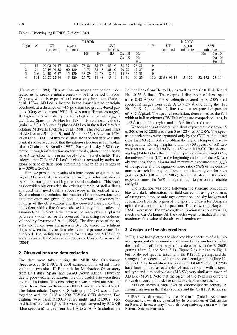
Fig. 2. As Fig. 1 but for the spectra taken with the R1200Y grating, the strongest flare detected using this spectral configuration (flare 12, seeSect. 3.1), and the reference star GJ 725B.

observed even in its quiescent state (see Figs. 1 and 2). The great-est emission in these lines is found at the maximum of the de-tected flares. The He i D3 and He i 4026 Å lines also show emis-sion above the continuum, which is more noticeable during thestrongest flares. The Na iD1 & D2 absorption lines only present aslight filled-in profile in the quiescent state, although a low emis-sion is observed in their core during flares. High resolution spec-troscopic observations of the quiescent state of AD Leo confirmthe presence of chromospheric emission lines that range froma weak emission in the center of the Ca ii IRT and the Na i D1& D2 lines to a strong emission in the He i D3, Mg ii h & k,Ca ii H & K and H i Balmer lines (Pettersen & Coleman 1981;Doyle 1987; Crespo-Chacón et al. 2006). In addition, Sundlandet al. (1988) suggested that Balmer lines are the most importantcomponents of chromospheric radiation loss.

AD Leo is well-known for having strong flares (see, for ex-ample, Hawley & Pettersen 1991). However, after overlappingthe normalized spectra and comparing the depth of the absorp-tion lines and the shape of the continuum, we have not de-tected any noticeable continuum change (see also Figs. 1 and 2).Therefore the flares analyzed in this work are non white-lightflares and, within the studied wavelength range, they only af-fect the emission in the chromospheric lines. Even though thiskind of flare is the most typical in the Sun, in which no de-tectable signature in white-light is generally observed, very fewsuch events had been detected previously in stars (see Butleret al. 1986; Houdebine 2003). Conversely to the Sun, stellar nonwhite-light flares seldom have been observed because very lit-tle time has been dedicated to spectroscopy in comparison tophotometry. However, Houdebine (1992) suggested that the low


Table 2. Minimum and maximum relative error in the EW of the different chromospheric lines.

Night �EWrel (%)(min–max)

Hβ Hγ Hδ He i λ4026 Å Ca ii K Ca ii H+Hε H8 H9 H10 H11 Hα Na i D1 Na i D2 He i D3

1 10–13 6–9 8–14 20–46 5–8 5–8 9–20 9–17 11–24 16–37 – – – –2 9–15 6–10 7–17 19–57 5–9 5–10 9–23 9–22 12–34 17–62 – – – –3 10–17 6–12 8–20 24–109 5–13 5–13 10–28 9–29 12–41 17–61 – – – –4 10–20 6–15 8–23 27–152 5–14 6–15 10–34 10–39 12–56 18–145 9–20 2–5 1–5 32–328

frequency observed for stellar non white-light flares could be dueto a strong contrast effect. In other words, many flares have beendetected as white-light flares on dMe stars because of the rela-tive weakness of their photospheric background, but they wouldhave been classified as non white-light flares on the Sun becauseof its much higher photospheric background.

3.1. Equivalent widths

The equivalent width (EW) of the observed chromospheric lineshas been measured very carefully in order to detect possibleweak flares in our observations. Two methods have been used.The first one consists of obtaining the EW with the routineSPLOT included in IRAF, taking the same wavelength limits foreach line in all the spectra. The second method uses the rou-tine SBANDS of IRAF, which generally introduces less noisein the EW measurement because it takes into account a largernumber of points to calculate the continuum value. For this rea-son, we only present the results obtained with SBANDS. Notethat the line regions have been taken wide enough to include theenhancement of the line wings during flares.

SBANDS uses Eq. (1) to obtain the EW of a line: Wl is thewidth at the base of the line, d is the reciprocal dispersion (pixelsize in Å), Fc,i is the flux per pixel in the continuum under theline, Fl,i is the observed flux in the pixel i of the line, and n is thenumber of pixels within the line region.

EW = Wl − dFc,i

i=n∑i=1

Fl,i . (1)

The EW uncertainty has been estimated using Eq. (2). We haveconsidered �Wl = 0 Å and �d = 0.01 Å/pixel. Equation (2) hasbeen obtained by applying the standard quadratic error propa-gation theory to Eq. (1), taking into account that n = Wl/d andassuming �Fl,i ≈ �Fc,i = Fc,i/SNR.

�EW =√

(C1)2 + (C2)2 + (C3)2 + (C4)2 (2)

where

C1 =∂EW∂Wl�Wl = �Wl

C2 =∂EW∂d�d =

EW −Wl

d�d

C3 =∂EW∂Fc,i�Fc,i =

Wl − EWSNR

C4 =∂EW∂Fl,i�Fl,i =

√Wl d

SNR·

Table 2 shows the minimum and maximum values of the rela-tive error in EW (�EWrel) for each chromospheric line and each

night. The �EWrel of the Ca ii H & K, Na i D1 & D2, Hβ, Hγand Hδ lines is between 1% and 20%. For H8 and H9 the �EWrelis less than 40%, while for H10 and H11 is higher than the un-certainty estimated for the other Balmer lines (up to 50% in thecase of H10 and even larger than 100% in the case of H11). The�EWrel of He i D3 and He i 4026 Å is frequently greater than100%. For this reason, the results obtained for the He i lines areless reliable. In addition, because of the short exposure times andthe relative faintness of AD Leo in the blue, the region bluewardof H10 is usually too noisy for reliable measurements.

The observed flares have been detected using the Hβ and Hαlines (for the blue and red spectra, respectively). Hβ and Hαwerechosen because they suffer from large variations during flaresand are the chromospheric lines with the best SNR in each spec-tral configuration.

Figure 3 shows the temporal evolution found for the EW ofthe Hβ line. The observed flares are marked with numbers. Othersmaller changes can also be seen. The temporal evolution foundfor the EW of the Hα line is given in Fig. 4. No strong varia-tions have been observed during our spectroscopic monitoring.However, 14 short and weak flares have been detected: 11 amongthe blue spectra and 3 among the red ones. The Julian Date (JD)at the beginning of each flare (JDstart) is shown in Table 3. Theseflares also have been observed in the other chromospheric lines.Nevertheless, it is more difficult to distinguish between flaresand noise for lower SNR and/or weaker lines. In addition, a mod-ulation with a period of ∼2 days is also observed in the quiescentemission of AD Leo, although the photometric period of this starwas found to be 2.7 days (Spiesman & Hawley 1986).

The flare frequency is very high, and sometimes new flarestake place when others are still active (see, for example, flares 8and 11 and the points before flares 2 and 7 in Fig. 3). Notealso that the flares on night 4 seem to erupt over the grad-ual decay phase of another stronger flare (Fig. 4). To calcu-late the flare frequency we have taken the total observed timeas the sum of UTend – UTstart for all the nights (see Table 1).Note that, within a night, the series of observations are notcontinuous in time. Therefore the flare frequency should begreater than the obtained one. This implies that the flare activ-ity of AD Leo, found from the variations of the chromosphericemission lines, is >0.71 flares/h. This value is slightly higherthan those that other authors measured by using photometry:Moffett (1974) observed 0.42 flares/h, Pettersen et al. (1984) de-tected 0.57 flares/h, and Konstantinova-Antova & Antov (1995)found 0.33−0.70 flares/h. Given that the detected flares are nonwhite-light flares, we conclude that non white-light flares maybe more frequent on stars than white-light flares as observed onthe Sun. As the total time of the gaps between the series of obser-vations is similar to the total real observed time, the flare activityof AD Leo could even double that obtained. As far as we know,this is the first time that such a high flare frequency is inferredfrom the variation of the chromospheric emission lines.


Fig. 3. Temporal evolution of the EW of the Hβ line. The strongest observed flares are labeled.

Table 3. JD of the flare onset (JDstart), total duration of the detected flares and length of their phases (seen in the Hβ line in the case of flares 1to 11 and seen in the Hα line in the case of flares 12 to 14). The time delay between the maximum of the chromospheric lines and the one of Hβor Hα, depending on the spectral configuration, is also shown. Blanks are given when the beginning, maximum and/or end of the flare was notobserved in the line under consideration.

Flare JDstart (days) Duration (min) Delay of the maximum (min)(2 452 000+)

Total Impulsive phase Gradual decay Ca ii K He i 4026 Å(Hβ) (Hβ) (Hβ)

1 2.513 ± 0.003 – 13 ± 7 – – 0 ± 62 3.3903 ± 0.0016 25 ± 4 11 ± 5 14 ± 4 0 ± 5 0 ± 53 3.5321 ± 0.0016 – 10 ± 4 – 0 ± 4 0 ± 44 3.5608 ± 0.0013 31 ± 3 10 ± 4 22 ± 3 0 ± 4 0 ± 45 4.3781 ± 0.0010 18 ± 4 6 ± 2 11 ± 3 0 ± 1 –6 4.4193 ± 0.0005 22 ± 1 4 ± 2 17 ± 2 5 ± 3 0 ± 37 4.4804 ± 0.0010 25 ± 2 9 ± 3 16 ± 2 3 ± 2 1 ± 28 4.5479 ± 0.0009 – 10 ± 2 – 1 ± 1 1 ± 19 4.5978 ± 0.0005 17 ± 2 5 ± 1 12 ± 2 2 ± 1 –

10 – – – – – –11 5.3968 ± 0.0005 14 ± 1 1 ± 1 12 ± 1 3 ± 1 –

Flare JDstart (days) Duration (min) Delay of the maximum (min)(2 452 000+)

Total Impulsive phase Gradual decay Na i D1, D2 He i D3

(Hα) (Hα) (Hα)12 5.5341 ± 0.0003 31 ± 2 5.9 ± 0.9 25 ± 2 0.9 ± 0.9 –13 5.5763 ± 0.0005 14 ± 1 2 ± 1 12 ± 1 1 ± 1 1 ± 114 – – – – – –

3.2. Equivalent widths relative to the quiescent state

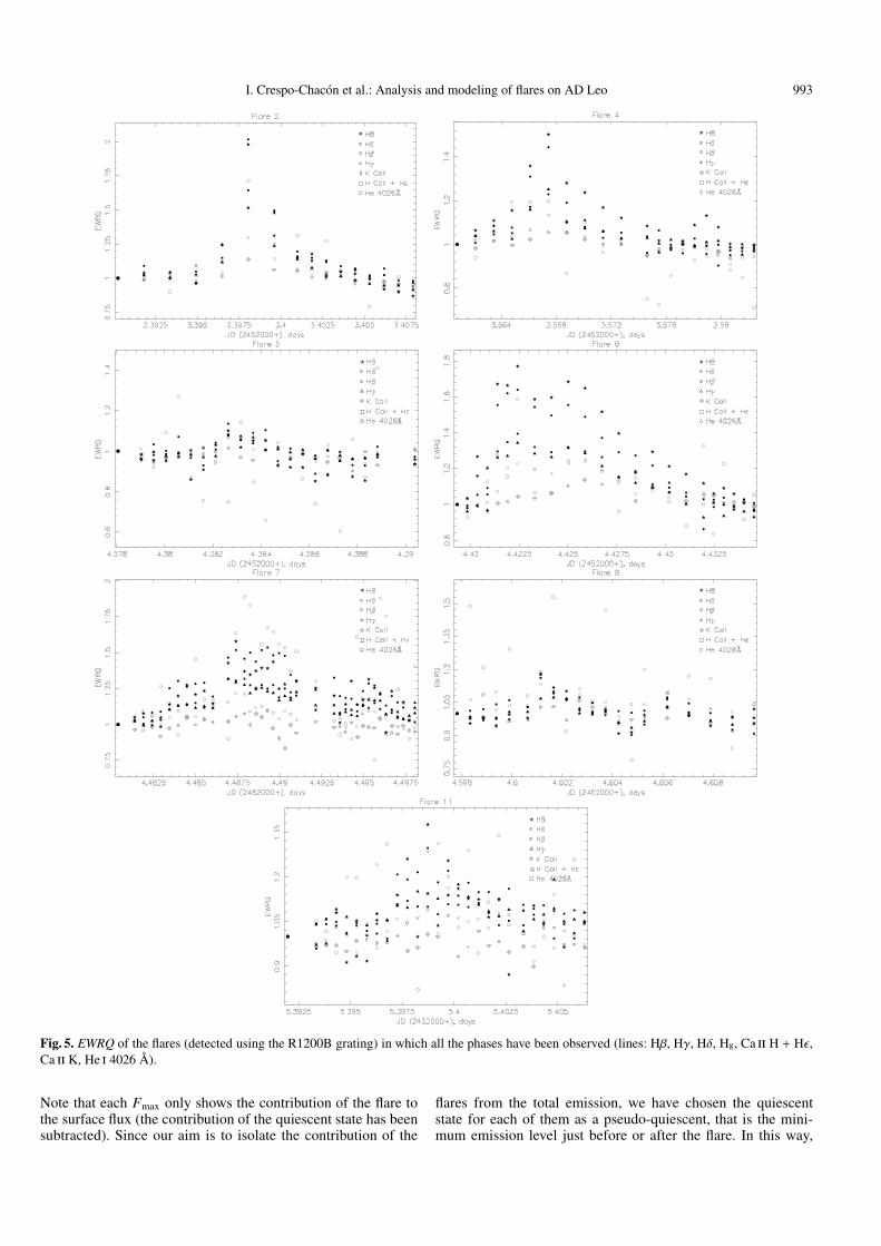
In order to compare the behaviour of the different chromosphericlines, we have used the equivalent width relative to the quies-cent state (EWRQ), defined as the ratio of the EW to the EW inthe quiescent state. Figures 5 and 6 show the EWRQ of severallines for a representative sample of the detected flares (those inwhich all the phases have been observed). The chromosphericlines plotted in these two figures are those with less uncertaintyin the EW measurement. We can observe two different kinds offlares: for some of them (see flares 6, 9, 11, 12 and 13) the grad-ual decay phase of the Balmer lines is much longer than the im-pulsive phase; in contrast, other flares (2, 4, 5 and 7) are lessimpulsive. This resembles the classification of solar flares madeby Pallavicini et al. (1977): eruptive flares or long-decay eventsand confined or compact flares. However, all these flares always

show the same behaviour in the Ca ii H & K lines, that is, a slowevolution throughout all the event. The evolution of the Na i D1

& D2, He i D3 and He i 4026 Å lines is quite similar to that of theBalmer series. However, it is less clear for the He i lines becausesometimes they have a very high error.

In some flares (5, 6, 11, 12 and 13) we can see two max-ima in the Na i and Balmer lines, but it is not so evident for theHe i and Ca ii lines. Sometimes variations on shorter time scalesare also detected during the gradual decay phase, in which dif-ferent peaks, decreasing in intensity, are observed in the EWRQ(see, for instance, flare 12). This could be interpreted as the suc-cession of different reconnection processes, decreasing in effi-ciency, within the same flare – following the original suggestionof Kopp & Pneuman (1976) – or as a series of flares occuring asa result of wave disturbances along the stellar surface from thefirst flare region.


Table 4. EWRQ at flare maximum (EWRQmax) for the different chromospheric lines. Blanks are given when the flare maximum was not detectedin the line under consideration. Flares with no maximum data in any line have been omitted.

Flare EWRQmax

Hβ Hγ Hδ H8 H9 H10 H11 Ca ii H + Hε Ca ii K He i 4026 Å1 1.26 ± 0.18 1.28 ± 0.11 1.47 ± 0.17 1.53 ± 0.22 1.52 ± 0.20 1.7 ± 0.3 1.6 ± 0.4 1.16 ± 0.09 – 1.5 ± 0.52 1.65 ± 0.25 1.52 ± 0.14 2.0 ± 0.3 2.0 ± 0.3 1.8 ± 0.3 1.5 ± 0.3 2.0 ± 0.7 1.30 ± 0.11 1.14 ± 0.09 1.7 ± 0.63 1.09 ± 0.19 1.06 ± 0.10 1.10 ± 0.17 1.11 ± 0.21 1.13 ± 0.22 0.99 ± 0.23 1.0 ± 0.4 1.1 ± 0.1 1.01 ± 0.09 1.3 ± 0.54 1.23 ± 0.20 1.25 ± 0.12 1.44 ± 0.21 1.5 ± 0.3 1.5 ± 0.3 1.6 ± 0.3 1.6 ± 0.6 1.13 ± 0.10 1.06 ± 0.09 1.2 ± 0.55 1.08 ± 0.20 1.08 ± 0.13 1.14 ± 0.21 1.1 ± 0.3 1.1 ± 0.3 1.0 ± 0.3 1.5 ± 0.6 1.06 ± 0.13 1.01 ± 0.12 –6 1.4 ± 0.3 1.34 ± 0.17 1.6 ± 0.3 1.8 ± 0.5 1.4 ± 0.4 1.5 ± 0.5 1.3 ± 0.5 1.23 ± 0.16 1.14 ± 0.13 1.6 ± 0.97 1.32 ± 0.24 1.32 ± 0.17 1.5 ± 0.3 1.4 ± 0.4 1.7 ± 0.4 1.5 ± 0.5 1.9 ± 0.8 1.15 ± 0.15 1.09 ± 0.14 1.9 ± 1.18 1.27 ± 0.23 1.25 ± 0.14 1.49 ± 0.25 1.5 ± 0.3 1.5 ± 0.3 1.4 ± 0.4 1.5 ± 0.6 1.16 ± 0.13 1.06 ± 0.11 1.6 ± 0.89 1.16 ± 0.21 1.07 ± 0.13 1.18 ± 0.21 1.2 ± 0.3 1.3 ± 0.3 1.1 ± 0.3 1.0 ± 0.4 1.13 ± 0.14 1.06 ± 0.14 –11 1.12 ± 0.22 1.10 ± 0.15 1.19 ± 0.24 1.3 ± 0.3 1.1 ± 0.3 1.2 ± 0.4 1.0 ± 0.5 1.05 ± 0.13 1.07 ± 0.13 –

Flare EWRQmax

Hα Na i D1 Na i D2 He i D3

12 1.09 ± 0.15 0.95 ± 0.04 0.95 ± 0.03 –13 1.13 ± 0.18 0.98 ± 0.04 0.98 ± 0.04 1.5 ± 1.1

Fig. 4. As Fig. 3 but for the Hα line. The observed flares have beennumbered following the order in Fig. 3.

Table 3 contains the total duration of the detected flares, thelength of their impulsive and gradual decay phases, and the timedelay between the maximum of each chromospheric line and thatof Hβ or Hα (depending on the spectral configuration). The de-tected flares last from 14 ± 1 to 31 ± 3 min. Regarding the firstmaximum of emission, we have found that the Balmer seriesreach it simultaneously while the rest of the lines are delayed.The delay is negligible for the He i and Na i lines (∼1 min) but itis very evident for Ca ii H & K (up to 5 ± 3 min). It seems thatthis delay is greater for the flares with a shorter impulsive phaseof the Balmer lines. However, the total duration of the flare doesnot seem to be related. For the first five flares, we cannot as-sume that the delay of the maximum is completely zero becausetheir uncertainties, particularly those of He i 4026 Å, are evengreater than the delay found in the other cases. The moment atwhich a line reaches its maximum is related to the height wherethe line is formed above the stellar surface. This is also relatedto the temperature that characterizes the formation of the line.According to the line formation models in stellar atmospheres,the Ca ii H & K lines are formed at deeper and cooler layers

than the Balmer series. Therefore, the gas that is heated andevaporated into the newly formed loop after magnetic reconnec-tion (Cargill & Priest 1983; Forbes & Malherbe 1986) cools andreaches the formation temperature of the Balmer series beforethe one of the Ca ii H & K lines. Houdebine (2003) found thatthe rise and decay times in the Ca ii K and Hγ lines obey goodrelationships, which implies that there is a well-defined under-lying mechanism responsible for the flux time profiles in theselines.

Table 4 lists the EWRQ of the chromospheric lines at theirmaximum in each flare (EWRQmax). The lower the wavelength,the greater EWRQmax is found for the Balmer lines. However,Hβ and Hγ have a very similar variation. For He i 4026 Å andHe i D3 the EWRQmax is analogous to that of the Balmer series,whereas for the Ca ii H & K and Na i D1 & D2 lines is smaller.Our results show that the duration of flares tends to be largerwhen the EWRQmax of the Balmer lines is greater. This effect ismore noticeable for the less impulsive flares. Nevertheless, thereare no clear relationships between the EWRQmax of the otherlines and the duration of the flare.

3.3. Line fluxes and released energy

In order to estimate the flare energy released in the observedchromospheric lines, we have converted the EW into absolutesurface fluxes and luminosities.

The absolute line fluxes (F) have been computed from theEW measured for each line and its local continuum. The abso-lute flux of the continuum near each line has been determinedmaking use of the method given by Pettersen & Hawley (1989).For AD Leo, they interpolate between the R and I filter pho-tometric fluxes to estimate the observed flux in the continuumnear 8850 Å. This value is then transformed into a continuumsurface flux of F(8850 Å) = 6.5 × 105 erg s−1 cm−2 Å−1, using0.44 R� for the radius and 0.203 arcsec for the parallax. Directscaling from the flux-calibrated spectrum of AD Leo, shownby Pettersen & Hawley (1989), has allowed us to estimate thecontinuum surface fluxes near the emission lines of interest. Wemultiply this continuum value by the measured EW to determinethe line surface flux. The absolute fluxes of the Balmer lines atthe different flare maxima (Fmax) are listed in Table 5. These val-ues will be used in Sect. 4 to calculate the Balmer decrements.


Fig. 5. EWRQ of the flares (detected using the R1200B grating) in which all the phases have been observed (lines: Hβ, Hγ, Hδ, H8, Ca ii H + Hε,Ca ii K, He i 4026 Å).

Note that each Fmax only shows the contribution of the flare tothe surface flux (the contribution of the quiescent state has beensubtracted). Since our aim is to isolate the contribution of the

flares from the total emission, we have chosen the quiescentstate for each of them as a pseudo-quiescent, that is the mini-mum emission level just before or after the flare. In this way,


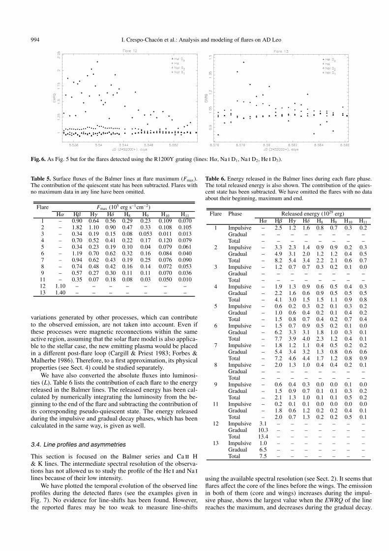
Fig. 6. As Fig. 5 but for the flares detected using the R1200Y grating (lines: Hα, Na i D1, Na i D2, He i D3).

Table 5. Surface fluxes of the Balmer lines at flare maximum (Fmax).The contribution of the quiescent state has been subtracted. Flares withno maximum data in any line have been omitted.

Flare Fmax (105 erg s−1cm−2)Hα Hβ Hγ Hδ H8 H9 H10 H11

1 – 0.90 0.64 0.56 0.29 0.23 0.109 0.0702 – 1.82 1.10 0.90 0.47 0.33 0.108 0.1053 – 0.34 0.19 0.15 0.08 0.053 0.011 0.0134 – 0.70 0.52 0.41 0.22 0.17 0.120 0.0795 – 0.34 0.23 0.19 0.10 0.04 0.079 0.0616 – 1.19 0.70 0.62 0.32 0.16 0.084 0.0407 – 0.94 0.62 0.43 0.19 0.25 0.076 0.0908 – 0.74 0.48 0.42 0.16 0.14 0.072 0.0539 – 0.57 0.27 0.30 0.11 0.11 0.070 0.03611 – 0.35 0.07 0.18 0.08 0.03 0.050 0.01012 1.10 – – – – – – –13 1.40 – – – – – – –

variations generated by other processes, which can contributeto the observed emission, are not taken into account. Even ifthese processes were magnetic reconnections within the sameactive region, assuming that the solar flare model is also applica-ble to the stellar case, the new emitting plasma would be placedin a different post-flare loop (Cargill & Priest 1983; Forbes &Malherbe 1986). Therefore, to a first approximation, its physicalproperties (see Sect. 4) could be studied separately.

We have also converted the absolute fluxes into luminosi-ties (L). Table 6 lists the contribution of each flare to the energyreleased in the Balmer lines. The released energy has been cal-culated by numerically integrating the luminosity from the be-ginning to the end of the flare and subtracting the contribution ofits corresponding pseudo-quiescent state. The energy releasedduring the impulsive and gradual decay phases, which has beencalculated in the same way, is given as well.

3.4. Line profiles and asymmetries

This section is focused on the Balmer series and Ca ii H& K lines. The intermediate spectral resolution of the observa-tions has not allowed us to study the profile of the He i and Na ilines because of their low intensity.

We have plotted the temporal evolution of the observed lineprofiles during the detected flares (see the examples given inFig. 7). No evidence for line-shifts has been found. However,the reported flares may be too weak to measure line-shifts

Table 6. Energy released in the Balmer lines during each flare phase.The total released energy is also shown. The contribution of the quies-cent state has been subtracted. We have omitted the flares with no dataabout their beginning, maximum and end.

Flare Phase Released energy (1029 erg)Hα Hβ Hγ Hδ H8 H9 H10 H11

1 Impulsive – 2.5 1.2 1.6 0.8 0.7 0.3 0.2Gradual – – – – – – – –Total – – – – – – – –

2 Impulsive – 3.3 2.3 1.4 0.9 0.9 0.2 0.3Gradual – 4.9 3.1 2.0 1.2 1.2 0.4 0.5Total – 8.2 5.4 3.4 2.2 2.1 0.6 0.7









12 Impulsive 3.1 – – – – – – –Gradual 10.3 – – – – – – –Total 13.4 – – – – – – –

13 Impulsive 1.0 – – – – – – –Gradual 6.5 – – – – – – –Total 7.5 – – – – – – –

using the available spectral resolution (see Sect. 2). It seems thatflares affect the core of the lines before the wings. The emissionin both of them (core and wings) increases during the impul-sive phase, shows the largest value when the EWRQ of the linereaches the maximum, and decreases during the gradual decay.


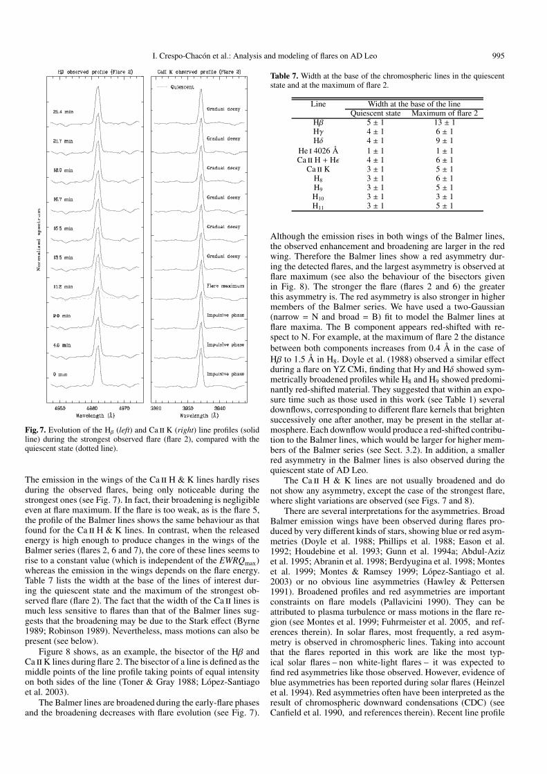
Fig. 7. Evolution of the Hβ (left) and Ca ii K (right) line profiles (solidline) during the strongest observed flare (flare 2), compared with thequiescent state (dotted line).

The emission in the wings of the Ca ii H & K lines hardly risesduring the observed flares, being only noticeable during thestrongest ones (see Fig. 7). In fact, their broadening is negligibleeven at flare maximum. If the flare is too weak, as is the flare 5,the profile of the Balmer lines shows the same behaviour as thatfound for the Ca ii H & K lines. In contrast, when the releasedenergy is high enough to produce changes in the wings of theBalmer series (flares 2, 6 and 7), the core of these lines seems torise to a constant value (which is independent of the EWRQmax)whereas the emission in the wings depends on the flare energy.Table 7 lists the width at the base of the lines of interest dur-ing the quiescent state and the maximum of the strongest ob-served flare (flare 2). The fact that the width of the Ca ii lines ismuch less sensitive to flares than that of the Balmer lines sug-gests that the broadening may be due to the Stark effect (Byrne1989; Robinson 1989). Nevertheless, mass motions can also bepresent (see below).

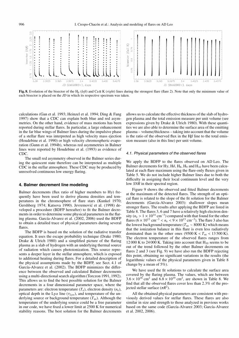
Figure 8 shows, as an example, the bisector of the Hβ andCa iiK lines during flare 2. The bisector of a line is defined as themiddle points of the line profile taking points of equal intensityon both sides of the line (Toner & Gray 1988; López-Santiagoet al. 2003).

The Balmer lines are broadened during the early-flare phasesand the broadening decreases with flare evolution (see Fig. 7).

Table 7. Width at the base of the chromospheric lines in the quiescentstate and at the maximum of flare 2.

Line Width at the base of the lineQuiescent state Maximum of flare 2

Hβ 5 ± 1 13 ± 1Hγ 4 ± 1 6 ± 1Hδ 4 ± 1 9 ± 1

He i 4026 Å 1 ± 1 1 ± 1Ca ii H + Hε 4 ± 1 6 ± 1

Ca ii K 3 ± 1 5 ± 1H8 3 ± 1 6 ± 1H9 3 ± 1 5 ± 1H10 3 ± 1 3 ± 1H11 3 ± 1 5 ± 1

Although the emission rises in both wings of the Balmer lines,the observed enhancement and broadening are larger in the redwing. Therefore the Balmer lines show a red asymmetry dur-ing the detected flares, and the largest asymmetry is observed atflare maximum (see also the behaviour of the bisectors givenin Fig. 8). The stronger the flare (flares 2 and 6) the greaterthis asymmetry is. The red asymmetry is also stronger in highermembers of the Balmer series. We have used a two-Gaussian(narrow = N and broad = B) fit to model the Balmer lines atflare maxima. The B component appears red-shifted with re-spect to N. For example, at the maximum of flare 2 the distancebetween both components increases from 0.4 Å in the case ofHβ to 1.5 Å in H8. Doyle et al. (1988) observed a similar effectduring a flare on YZ CMi, finding that Hγ and Hδ showed sym-metrically broadened profiles while H8 and H9 showed predomi-nantly red-shifted material. They suggested that within an expo-sure time such as those used in this work (see Table 1) severaldownflows, corresponding to different flare kernels that brightensuccessively one after another, may be present in the stellar at-mosphere. Each downflow would produce a red-shifted contribu-tion to the Balmer lines, which would be larger for higher mem-bers of the Balmer series (see Sect. 3.2). In addition, a smallerred asymmetry in the Balmer lines is also observed during thequiescent state of AD Leo.

The Ca ii H & K lines are not usually broadened and donot show any asymmetry, except the case of the strongest flare,where slight variations are observed (see Figs. 7 and 8).

There are several interpretations for the asymmetries. BroadBalmer emission wings have been observed during flares pro-duced by very different kinds of stars, showing blue or red asym-metries (Doyle et al. 1988; Phillips et al. 1988; Eason et al.1992; Houdebine et al. 1993; Gunn et al. 1994a; Abdul-Azizet al. 1995; Abranin et al. 1998; Berdyugina et al. 1998; Monteset al. 1999; Montes & Ramsey 1999; López-Santiago et al.2003) or no obvious line asymmetries (Hawley & Pettersen1991). Broadened profiles and red asymmetries are importantconstraints on flare models (Pallavicini 1990). They can beattributed to plasma turbulence or mass motions in the flare re-gion (see Montes et al. 1999; Fuhrmeister et al. 2005, and ref-erences therein). In solar flares, most frequently, a red asym-metry is observed in chromospheric lines. Taking into accountthat the flares reported in this work are like the most typ-ical solar flares – non white-light flares – it was expected tofind red asymmetries like those observed. However, evidence ofblue asymmetries has been reported during solar flares (Heinzelet al. 1994). Red asymmetries often have been interpreted as theresult of chromospheric downward condensations (CDC) (seeCanfield et al. 1990, and references therein). Recent line profile


Fig. 8. Evolution of the bisector of the Hβ (left) and Ca ii K (right) lines during the strongest flare (flare 2). Note that only the minimum value ofeach bisector is placed on the JD in which its respective spectrum was taken.

calculations (Gan et al. 1993; Heinzel et al. 1994; Ding & Fang1997) show that a CDC can explain both blue and red asym-metries. On the other hand, evidence of mass motions has beenreported during stellar flares. In particular, a large enhancementin the far blue wings of Balmer lines during the impulsive phaseof a stellar flare was interpreted as high velocity mass ejection(Houdebine et al. 1990) or high velocity chromospheric evapo-ration (Gunn et al. 1994b), whereas red asymmetries in Balmerlines were reported by Houdebine et al. (1993) as evidence ofCDC.

The small red asymmetry observed in the Balmer series dur-ing the quiescent state therefore can be interpreted as multipleCDC in the stellar atmosphere. These CDC may be produced byunresolved continuous low energy flaring.

4. Balmer decrement line modeling

Balmer decrements (flux ratio of higher members to Hγ) fre-quently have been used to derive plasma densities and tem-peratures in the chromosphere of flare stars (Kunkel 1970;Gershberg 1974; Katsova 1990). Jevremovic et al. (1998) de-veloped a procedure (BDFP hereafter) to fit the Balmer decre-ments in order to determine some physical parameters in the flar-ing plasma. García-Alvarez et al. (2002, 2006) used the BDFPto obtain a detailed trace of physical parameters during severalflares.

The BDFP is based on the solution of the radiative transferequation. It uses the escape probability technique (Drake 1980;Drake & Ulrich 1980) and a simplified picture of the flaringplasma as a slab of hydrogen with an underlying thermal sourceof radiation which causes photoionization. This source repre-sents a deeper layer in the stellar atmosphere, which is exposedto additional heating during flares. For a detailed description ofthe physical assumptions made by the BDFP, see Sect. 4.1 ofGarcía-Alvarez et al. (2002). The BDFP minimizes the differ-ence between the observed and calculated Balmer decrementsusing a multi-directional search algorithm (Torczon 1991, 1992).This allows us to find the best possible solution for the Balmerdecrements in a four dimensional parameter space, where theparameters are: electron temperature (Te), electron density (ne),optical depth in the Lyα line (τLyα), and temperature of the un-derlying source or background temperature (Tus). Although thetemperature of the underlying source could be a free parameterin our code, we have fixed a lower limit at 2500 K for numericalstability reasons. The best solution for the Balmer decrements

allows us to calculate the effective thickness of the slab of hydro-gen plasma and the total emission measure per unit volume (seeexpressions given by Drake & Ulrich 1980). With these quanti-ties we are also able to determine the surface area of the emittingplasma – volume/thickness – taking into account that the volumeis the ratio of the observed flux in the Hβ line to the total emis-sion measure (also in this line) per unit volume.

4.1. Physical parameters of the observed flares

We apply the BDFP to the flares observed on AD Leo. TheBalmer decrements for Hγ, Hδ, H8, H9 and H10 have been calcu-lated at each flare maximum using the flare-only fluxes given inTable 5. We do not include higher Balmer lines due to both thedifficulty in assigning their local continuum level and the verylow SNR in their spectral region.

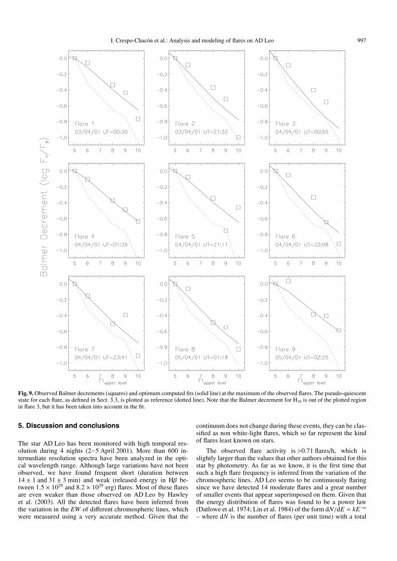
Figure 9 shows the observed and fitted Balmer decrementsat the maximum of the detected flares. The strength of an opti-cal flare is related to the slope of the fit solution for the Balmerdecrements (García-Alvarez 2003): shallower slopes meanstronger flares. The results after applying the BDFP are listed inTable 8. The flares 3, 6 and 7 have a relatively high electron den-sity (ne > 1 × 1014 cm−3) compared with that found for the otherflares (6 × 1013 cm−3 < ne < 9 × 1013 cm−3). The flare 3 also hasthe lowest background temperature (Tus ∼ 8000 K) which meansthat the ionization balance in this flare is even less radiativelydominated than in the other ones (9500 K < Tus < 13 500 K).The electron temperature of the observed flares ranges from12 000 K to 24 000 K. Taking into account that H10 seems to beout of the trend followed by the other Balmer decrements onflares 2 and 3 (see Fig. 9) we have also run the BDFP rejectingthis point, obtaining no significant variations in the results (thelogarithmic values of the physical parameters given in Table 8change by a mean of 5%).

We have used the fit solutions to calculate the surface areacovered by the flaring plasma. The values, which are between3.6 × 1018 cm2 and 6.8 × 1019 cm2, are shown in Table 8. Wefind that all the observed flares cover less than 2.3% of the pro-jected stellar surface (πR2).

All the obtained physical parameters are consistent with pre-viously derived values for stellar flares. These flares are alsosimilar in size and strength to those analyzed in previous worksbased on the same code (García-Alvarez 2003; García-Alvarezet al. 2002, 2006).


Fig. 9. Observed Balmer decrements (squares) and optimum computed fits (solid line) at the maximum of the observed flares. The pseudo-quiescentstate for each flare, as defined in Sect. 3.3, is plotted as reference (dotted line). Note that the Balmer decrement for H10 is out of the plotted regionin flare 3, but it has been taken into account in the fit.

5. Discussion and conclusions

The star AD Leo has been monitored with high temporal res-olution during 4 nights (2−5 April 2001). More than 600 in-termediate resolution spectra have been analyzed in the opti-cal wavelength range. Although large variations have not beenobserved, we have found frequent short (duration between14 ± 1 and 31 ± 3 min) and weak (released energy in Hβ be-tween 1.5 × 1029 and 8.2 × 1029 erg) flares. Most of these flaresare even weaker than those observed on AD Leo by Hawleyet al. (2003). All the detected flares have been inferred fromthe variation in the EW of different chromospheric lines, whichwere measured using a very accurate method. Given that the

continuum does not change during these events, they can be clas-sified as non white-light flares, which so far represent the kindof flares least known on stars.

The observed flare activity is >0.71 flares/h, which isslightly larger than the values that other authors obtained for thisstar by photometry. As far as we know, it is the first time thatsuch a high flare frequency is inferred from the variation of thechromospheric lines. AD Leo seems to be continuously flaringsince we have detected 14 moderate flares and a great numberof smaller events that appear superimposed on them. Given thatthe energy distribution of flares was found to be a power law(Datlowe et al. 1974; Lin et al. 1984) of the form dN/dE = kE−α– where dN is the number of flares (per unit time) with a total


Table 8. Physical parameters obtained for the observed flares. The area and stellar surface percentage covered by these flares are also shown.

Flare Date UT log τLyα log ne log Te log Tus Area Surface(×1019 cm2) (%)

1 03/04/01 00:30 3.71 13.75 4.31 4.13 1.17 0.402 03/04/01 21:32 4.62 13.79 4.07 3.99 6.79 2.303 04/04/01 00:55 4.18 14.22 4.09 3.90 1.45 0.494 04/04/01 01:36 3.78 13.95 4.30 3.98 0.89 0.305 04/04/01 21:11 4.54 13.79 4.12 4.02 0.76 0.266 04/04/01 22:08 4.43 14.12 4.07 4.04 3.14 1.077 04/04/01 23:41 4.41 14.39 4.09 4.02 2.13 0.728 05/04/01 01:18 4.15 13.78 4.17 3.98 2.12 0.729 05/04/01 02:25 3.60 13.88 4.38 4.09 0.36 0.12

energy (thermal or radiated) in the interval [E, E + dE], and α isgreater than 0 – we can expect very weak flares occurring evenmore frequently than the observed ones. Therefore our resultscan be interpreted as additional evidence of the important rolethat flares can play as heating agents of the outer atmosphericstellar layers (Güdel 1997; Audard et al. 2000; Kashyap et al.2002; Güdel et al. 2003; Arzner & Güdel 2004).

A total of 14 flares have been studied in detail. The Balmerlines allow us to distinguish two different morphologies: someflares show a gradual decay much longer than the impulsivephase while another ones are less impulsive. This resembles thetwo main types of solar flares (eruptive and confined) describedby Pallavicini et al. (1977). However, the Ca ii H & K lines al-ways show the same behaviour and their evolution is less impul-sive than that found for the Balmer lines. The two maxima and/orweak peaks, observed sometimes during the detected flares, canbe interpreted as the succession of different magnetic reconnec-tion processes, which would be caused as consequence of thedisturbance produced by the original flare, as Kopp & Pneuman(1976) suggested for the Sun. The Ca ii H & K lines reach theflare maximum after the Balmer series. It seems that the timedelay is higher when the impulsive phase of the Balmer lines isshorter. The moment at which a line reaches its maximum is re-lated to the temperature that characterizes the formation of theline and, therefore, is also related to the height where the lineis formed. During the detected flares, the relative increase ob-served in the emission of the Balmer lines is greater for lowerwavelengths. We have also found that not only are the detectedflares like the most typical solar flares (non white-light flares),but the asymmetries observed in chromospheric lines (red asym-metries) are also like the most frequent asymmetries observedin the Sun during flares. The detected broad Balmer emissionwings and red asymmetries can be attributed to plasma turbu-lence, mass motions or CDC. The Ca ii H & K lines seem to beless affected by flare events and their broadening is negligible. Asmall red asymmetry in the Balmer series is also observed dur-ing the quiescent state, which could be interpreted as multipleCDC probably due to continuous flaring of very low energy.

We have used the Balmer decrements as a tracer of physi-cal parameters during flares by using the model developed byJevremovic et al. (1998). The physical parameters of the flar-ing plasma (electron density, electron temperature, optical thick-ness and temperature of the underlying source), as well as thecovered stellar surface, have been obtained. The electron den-sities found for the analyzed flares (6 × 1013−2 × 1014 cm−3)are in general agreement with those that other authors findby using semi-empirical chromospheric modeling (Hawley &Fisher 1992a,b; Mauas & Falchi 1996). The electron temper-atures are between 12 000 K and 24 000 K. The temperature ofthe background source ranges from 8000 K to 13 500 K. All the

Fig. 10. Flare duration, stellar surface and temperature of the underlyingsource at flare maximum vs. energy released in Hβ during the detectedflares.

obtained physical parameters are consistent with previously de-rived values for stellar flares. The areas – no larger than 2.3%of the projected stellar surface – are comparable with the size ofother solar and stellar flares (Tandberg-Hanssen & Emslie 1988;García-Alvarez 2003; García-Alvarez et al. 2002, 2006).

We have also analyzed the relationships between the flareparameters. The released energy is correlated with the flare du-ration and the area covered by the flaring plasma, but not withthe temperature of the underlying source (see Fig. 10). Theseresults are in general agreement with those found by Hawleyet al. (2003) using only 4 flares and a different method for ob-taining the physical parameters. We have found a clear relationbetween the released energy and the flux at flare maximum (seeFig. 11). Also, the higher the flux, the longer the flare. This fluxis also correlated with the area covered by the emitting plasma atflare maximum, but not with the temperature of the underlyingsource (Fig. 11). No correlations between the area, temperatureand duration have been found: i.e. these parameters seem to beindependent. The magnetic geometry seems to be a very impor-tant factor in flares: firstly, the flare duration can be related tothe loop length, as in X-rays (see review by Reale 2002), in thesense that a fast decay implies a short loop and a slow decay


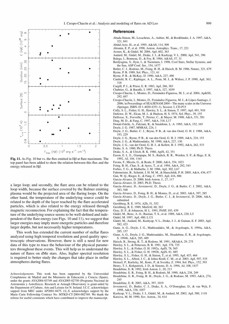
Fig. 11. As Fig. 10 but vs. the flux emitted in Hβ at flare maximum. Thetop panel has been added to show the relation between this flux and theenergy released in Hβ.

a large loop; and secondly, the flare area can be related to theloop width, because the surface covered by the Balmer emittingplasma would be the projected area of the flaring loops. On theother hand, the temperature of the underlying source could berelated to the depth of the layer reached by the flare acceleratedparticles, which is also related to the energy released throughmagnetic reconnection. For explaining the fact that the tempera-ture of the underlying source seems to be well-defined and inde-pendent of the flare energy (see Figs. 10 and 11), we suggest thatlarger energies may imply more energetic particles and thereforelarger depths, but not necessarily higher temperatures.

This work has extended the current number of stellar flaresanalyzed using high temporal resolution and good quality spec-troscopic observations. However, there is still a need for newdata of this type to trace the behaviour of the physical parame-ters throughout these events. This will help us to understand thenature of flares on dMe stars. Also, higher spectral resolutionis required to better study the changes that take place in stellaratmospheres during flares.

Acknowledgements. This work has been supported by the UniversidadComplutense de Madrid and the Ministerio de Educación y Ciencia (Spain),under the grants AYA2004-03749 and AYA2005-02750 (Programa Nacional deAstronomía y Astrofísica). Research at Armagh Observatory is grant-aided bythe Department of Culture, Arts and Leisure for N. Ireland. I.C.C. acknowledgessupport from MEC under AP2001-0475. J.L.S. acknowledges support by theMarie Curie Fellowship Contract No. MTKD-CT-2004-002769. We thank thereferee for useful comments which have contributed to improve the manuscript.

ReferencesAbada-Simon, M., Lecacheux, A., Aubier, M., & Bookbinder, J. A. 1997, A&A,

321, 841Abdul-Aziz, H., et al. 1995, A&AS, 114, 509Abranin, E. P., et al. 1998, Astron. Astrophys. Trans., 17, 221Arzner, K., & Güdel, M. 2004, ApJ, 602, 363Audard, M., Güdel, M., Drake, J. J., & Kashyap, V. L. 2000, ApJ, 541, 396Balega, I., Bonneau, D., & Foy, R. 1984, A&AS, 57, 31Berdyugina, S., Ilyin, I., & Tuominen, I. 1998, Cool Stars, Stellar Systems, and

the Sun, ASP Conf. Ser., 154, 1477Butler, C. J., Rodono, M., Foing, B. H., & Haisch, B. M. 1986, Nature, 321, 679Byrne, P. B. 1989, Sol. Phys., 121, 61Byrne, P. B., & McKay, D. 1990, A&A, 227, 490Canfield, R. C., Kiplinger, A. L., Penn, M. J., & Wülser, J. P. 1990, ApJ, 363,

318Cargill, P. J., & Priest, E. R. 1983, ApJ, 266, 383Chabrier, G., & Baraffe, I. 1997, A&A, 327, 1039Crespo-Chacón, I., Montes, D., Fernández-Figueroa, M. J., et al. 2004, Ap&SS,

292, 697Crespo-Chacón, I., Montes, D., Fernández-Figueroa, M. J., & López-Santiago, J.

2006, in Proceedings of SEA/JENAM 2004 – The many scales in the Universe(Springer, ISBN-10 1-4020-4351-1), Session 3, CD-P15

Cully, S. L., Fisher, G. H., Hawley, S. L., & Simon, T. 1997, ApJ, 491, 910Datlowe, D. W., Elcan, M. J., & Hudson, H. S. 1974, Sol. Phys., 39, 155Delfosse, X., Forveille, T., Perrier, C., & Mayor, M. 1998, A&A, 331, 581Ding, M. D., & Fang, C. 1997, A&A, 318, L17Donati-Falchi, A., Falciani, R., & Smaldone, L. A. 1985, A&A, 152, 165Doyle, J. G. 1987, MNRAS, 224, 1Doyle, J. G., Butler, C. J., Bryne, P. B., & van den Oord, G. H. J. 1988, A&A,

193, 229Doyle, J. G., Byrne, P. B., & van den Oord, G. H. J. 1989, A&A, 224, 153Doyle, J. G., & Mathioudakis, M. 1990, A&A, 227, 130Doyle, J. G., van der Oord, G. H. J., & Kellett, B. J. 1992, A&A, 262, 533Drake, S. A. 1980, Ph.D. ThesisDrake, S. A., & Ulrich, R. K. 1980, ApJS, 42, 351Eason, E. L. E., Giampapa, M. S., Radick, R. R., Worden, S. P., & Hege, E. K.

1992, AJ, 104, 1161Favata, F., Micela, G., & Reale, F. 2000, A&A, 354, 1021Foing, B. H., Char, S., & Ayres, T., et al. 1994, A&A, 292, 543Forbes, T. G., & Malherbe, J. M. 1986, ApJ, 302, L67Fuhrmeister, B., Schmitt, J. H. M. M., & Hauschildt, P. H. 2005, A&A, 436, 677Gan, W. Q., Rieger, E., & Fang, C. 1993, ApJ, 416, 886Garcia-Alvarez, D. 2000, Irish Astron. J., 27, 117Garcia-Alvarez, D. 2003, Ph.D. ThesisGarcía-Alvarez, D., Jevremovic, D., Doyle, J. G., & Butler, C. J. 2002, A&A,

383, 548García-Alvarez, D., Foing, B. H., & Montes, D., et al. 2003, A&A, 397, 285García-Alvarez, D., Doyle, J. G., Butler, C. J., & Jevremovic, D. 2006, A&A,

submittedGershberg, R. E. 1974, AZh, 51, 552Gershberg, R. E. 1989, MmSAI, 60, 263Gray, D. F., & Johanson, H. L. 1991, PASP, 103, 439Güdel, M., Benz, A. O., Bastian, T. S., et al. 1989, A&A, 220, L5Güdel, M. 1997, ApJ, 480, L121Güdel, M., Audard, M., Kashyap, V. L., Drake, J. J., & Guinan, E. F. 2003, ApJ,

582, 423Gunn, A. G., Doyle, J. G., Mathioudakis, M., & Avgoloupis, S. 1994a, A&A,

285, 157Gunn, A. G., Doyle, J. G., Mathioudakis, M., Houdebine, E. R., & Avgoloupis,

S. 1994b, A&A, 285, 489Haisch, B., Strong, K. T., & Rodono, M. 1991, ARA&A, 29, 275Hawley, S. L., & Pettersen, B. R. 1991, ApJ, 378, 725Hawley, S. L., & Fisher, G. H. 1992a, ApJS, 78, 565Hawley, S. L., & Fisher, G. H. 1992b, ApJS, 81, 885Hawley, S. L., Fisher, G. H., & Simon, T., et al. 1995, ApJ, 453, 464Hawley, S. L., Allred, J. C., & Johns-Krull, C. M., et al. 2003, ApJ, 597, 535Heinzel, P., Karlicky, M., Kotrc, P., & Svestka, Z. 1994, Sol. Phys., 152, 393Henry, T. J., Kirkpatrick, J. D., & Simons, D. A. 1994, AJ, 108, 1437Houdebine, E. R. 1992, Irish Astron. J., 20, 213Houdebine, E. R., Foing, B. H., & Rodonò, M. 1990, A&A, 238, 249Houdebine, E. R., Foing, B. H., Doyle, J. G., & Rodono, M. 1993, A&A, 274,

245Houdebine, E. R. 2003, A&A, 397, 1019Jevremovic, D., Butler, C. J., Drake, S. A., O’Donoghue, D., & van Wyk, F.

1998, A&A, 338, 1057Kashyap, V. L., Drake, J. J., Güdel, M., & Audard, M. 2002, ApJ, 580, 1118Katsova, M. M. 1990, Sov. Astron., 34, 614


Konstantinova-Antova, R. K., & Antov, A. P. 1995, in Proc. IAU Coll., 151,Lecture Notes in Physics (Berlin: Springer Verlag), 454, 87

Kopp, R. A., & Pneuman, G. W. 1976, Sol. Phys., 50, 85Kunkel, W. E. 1970, ApJ, 161, 503Lang, K. R., & Willson, R. F. 1986, ApJ, 305, 363Lin, R. P., Schwartz, R. A., Kane, S. R., Pelling, R. M., & Hurley, K. C. 1984,

ApJ, 283, 421López-Santiago, J., Montes, D., Fernández-Figueroa, M. J., & Ramsey, L. W.

2003, A&A, 411, 489Maggio, A., Drake, J. J., Kashyap, V., et al. 2004, ApJ, 613, 548Mauas, P. J. D., & Falchi, A. 1996, A&A, 310, 245Mirzoyan, L. V. 1984, Vistas Astron., 27, 77Moffett, T. J. 1974, ApJS, 29, 1Montes, D., & Ramsey, L. W. 1999, Solar and Stellar Activity: Similarities and

Differences, ASP Conf. Ser., 158, 226Montes, D., Saar, S. H., Collier Cameron, A., & Unruh, Y. C. 1999, MNRAS,

305, 45Montes, D., Crespo-Chacón, I., Fernández-Figueroa, J., & García Alvarez, D.

2003, IAU Symp., 219, CD-910Pallavicini, R. 1990, in Basic plasma processes on the sun, IAU Symp., 142, 77Pallavicini, R., Serio, S., & Vaiana, G. S. 1977, ApJ, 216, 108Pettersen, B. R. 1976, Institute of Theoretical Astrophysics Blindern Oslo

Reports, 46, 1Pettersen, B. R. 1989, Sol. Phys., 121, 299Pettersen, B. R., & Coleman, L. A. 1981, ApJ, 251, 571Pettersen, B. R., & Hawley, S. L. 1989, A&A, 217, 187Pettersen, B. R., Coleman, L. A., & Evans, D. S. 1984, ApJS, 54, 375

Pettersen, B. R., Panov, K. P., & Ivanova, M. S., et al. 1990, in Flare Stars in StarClusters, Associations and the Solar Vicinity, IAU Symp., 137, 15

Phillips, K. J. H., Bromage, G. E., Dufton, P. L., Keenan, F. P., & Kingston, A. E.1988, MNRAS, 235, 573

Reale, F. 2002, Stellar Coronae in the Chandra and XMM-NEWTON Era, ASPConf. Ser., 277, 103

Robinson, R. D. 1989, in Solar and Stellar Flares – Posters Papers, ed. B. M.Haisch, & M. Rodonò, 83

Robrade, J., & Schmitt, J. H. M. M. 2005, A&A, 435, 1073Rodonò, M., Houdebine, E. R., Catalano S., et al. 1989, in Solar and Stellar

Flares – Posters Papers, ed. B. M. Haisch, & M. Rodonò, 53Saar, S. H., & Linsky, J. L. 1985, ApJ, 299, L47Sanz-Forcada, J., & Micela, G. 2002, A&A, 394, 653Smith, K., Güdel, M., & Audard, M. 2005, A&A, 436, 241Spiesman, W. J., & Hawley, S. L. 1986, AJ, 92, 664Sundland, S. R., Pettersen, B. R., Hawley, S. L., Kjeldseth-Moe, O., & Andersen,

B. N. 1988, in Activity in Cool Star Envelopes, Astrophysics and SpaceScience Library (Dordrecht, Holland: D. Reidel Publishing Company, KluwerAcademic Publishers), 143, 61

Tandberg-Hanssen, E., & Emslie, A. G. 1988, in The physics of solar flares(Cambridge, New York: Cambridge University Press), 286

Toner, C., & Gray, D. F. 1988, ApJ, 334, 1008Torczon, V. 1991, SIAM J. Optimization, 1, 123Torczon, V. 1992, Tech. Report 92-9, Dep. of Mathematical Sciences, Rice

University, Houstonvan den Besselaar, E. J. M., Raassen, A. J. J., Mewe, R., et al. 2003, A&A, 411,

587

Documents

Astronomy c ESO 2006 Astrophysics - CORE · from La Palma (Spain) and SAAO (South Africa). However, due to poor weather conditions, the only useful data were those taken at La Palma