Astronomical Observational Techniques and Instrumentation

1

Astronomical Observational Techniques and Instrumentation

RIT Course Number 1060-771Professor Don Figer

Quantum-Limited Detectors

2

Aims for this lecture• Motivate the need for future detectors

• Describe physical principles of future detectors

• Review some promising technologies for future detectors

3

Motivation for Future Detectors

4

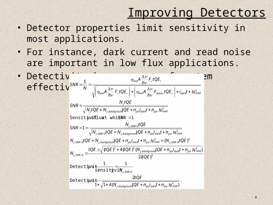
Improving Detectors• Detector properties limit sensitivity in most applications.

• For instance, dark current and read noise are important in low flux applications.

• Detectivity is a measure of system effectiveness.

.)(411

2yDetectivit

1

ysensitivit

1yDetectivit

)(2

)()(4)(

)(

1

1SNRat which flux y Sensitivit

2,

1,

2

2,

22

1,

21,

2,1,

2,1,

1,

2,

2,

NntintQEN

tQE

N

tQE

NntintQENtQEtQEtQEN

tQENNntintQENtQEN

NntintQENtQEN

tQENSNR

NntintQENtQEN

tQENSNR

NtitQEFh

AtQEFh

A

tQEFh

A

N

SSNR

readpixdarkpixbackground

SNR


SNR

SNRreadpixdarkpixbackgroundSNR

readpixdarkpixbackgroundSNR

SNR


readdarkbackinstinst

inst

5

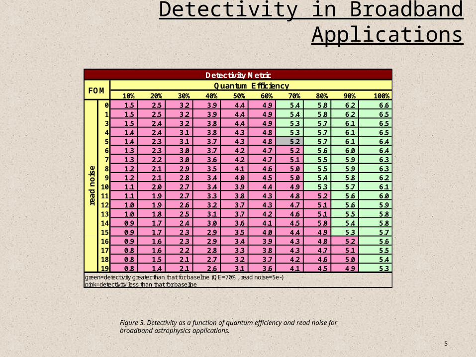
Detectivity in Broadband Applications

10% 20% 30% 40% 50% 60% 70% 80% 90% 100%0 1.5 2.5 3.2 3.9 4.4 4.9 5.4 5.8 6.2 6.6 1 1.5 2.5 3.2 3.9 4.4 4.9 5.4 5.8 6.2 6.5 3 1.5 2.4 3.2 3.8 4.4 4.9 5.3 5.7 6.1 6.5 4 1.4 2.4 3.1 3.8 4.3 4.8 5.3 5.7 6.1 6.5 5 1.4 2.3 3.1 3.7 4.3 4.8 5.2 5.7 6.1 6.4 6 1.3 2.3 3.0 3.7 4.2 4.7 5.2 5.6 6.0 6.4 7 1.3 2.2 3.0 3.6 4.2 4.7 5.1 5.5 5.9 6.3 8 1.2 2.1 2.9 3.5 4.1 4.6 5.0 5.5 5.9 6.3 9 1.2 2.1 2.8 3.4 4.0 4.5 5.0 5.4 5.8 6.2

10 1.1 2.0 2.7 3.4 3.9 4.4 4.9 5.3 5.7 6.1 11 1.1 1.9 2.7 3.3 3.8 4.3 4.8 5.2 5.6 6.0 12 1.0 1.9 2.6 3.2 3.7 4.3 4.7 5.1 5.6 5.9 13 1.0 1.8 2.5 3.1 3.7 4.2 4.6 5.1 5.5 5.8 14 0.9 1.7 2.4 3.0 3.6 4.1 4.5 5.0 5.4 5.8 15 0.9 1.7 2.3 2.9 3.5 4.0 4.4 4.9 5.3 5.7 16 0.9 1.6 2.3 2.9 3.4 3.9 4.3 4.8 5.2 5.6 17 0.8 1.6 2.2 2.8 3.3 3.8 4.3 4.7 5.1 5.5 18 0.8 1.5 2.1 2.7 3.2 3.7 4.2 4.6 5.0 5.4 19 0.8 1.4 2.1 2.6 3.1 3.6 4.1 4.5 4.9 5.3

read

no

ise

green=detectivity greater than that for baseline (QE=70%, read noise=5e-)pink=detectivity less than that for baseline

Detectivity Metric

FOMQuantum Efficiency

Figure 3. Detectivity as a function of quantum efficiency and read noise for broadband astrophysics applications.

6

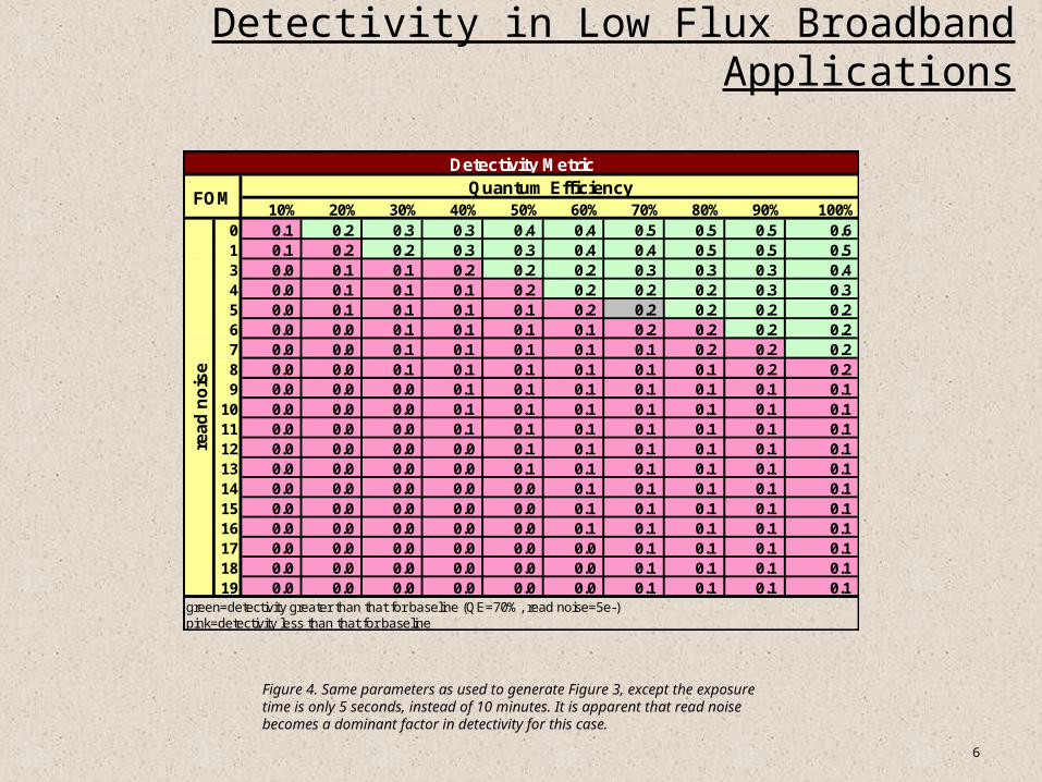
Detectivity in Low Flux Broadband Applications

10% 20% 30% 40% 50% 60% 70% 80% 90% 100%0 0.1 0.2 0.3 0.3 0.4 0.4 0.5 0.5 0.5 0.6 1 0.1 0.2 0.2 0.3 0.3 0.4 0.4 0.5 0.5 0.5 3 0.0 0.1 0.1 0.2 0.2 0.2 0.3 0.3 0.3 0.4 4 0.0 0.1 0.1 0.1 0.2 0.2 0.2 0.2 0.3 0.3 5 0.0 0.1 0.1 0.1 0.1 0.2 0.2 0.2 0.2 0.2 6 0.0 0.0 0.1 0.1 0.1 0.1 0.2 0.2 0.2 0.2 7 0.0 0.0 0.1 0.1 0.1 0.1 0.1 0.2 0.2 0.2 8 0.0 0.0 0.1 0.1 0.1 0.1 0.1 0.1 0.2 0.2 9 0.0 0.0 0.0 0.1 0.1 0.1 0.1 0.1 0.1 0.1

10 0.0 0.0 0.0 0.1 0.1 0.1 0.1 0.1 0.1 0.1 11 0.0 0.0 0.0 0.1 0.1 0.1 0.1 0.1 0.1 0.1 12 0.0 0.0 0.0 0.0 0.1 0.1 0.1 0.1 0.1 0.1 13 0.0 0.0 0.0 0.0 0.1 0.1 0.1 0.1 0.1 0.1 14 0.0 0.0 0.0 0.0 0.0 0.1 0.1 0.1 0.1 0.1 15 0.0 0.0 0.0 0.0 0.0 0.1 0.1 0.1 0.1 0.1 16 0.0 0.0 0.0 0.0 0.0 0.1 0.1 0.1 0.1 0.1 17 0.0 0.0 0.0 0.0 0.0 0.0 0.1 0.1 0.1 0.1 18 0.0 0.0 0.0 0.0 0.0 0.0 0.1 0.1 0.1 0.1 19 0.0 0.0 0.0 0.0 0.0 0.0 0.1 0.1 0.1 0.1

read

no

ise


Detectivity Metric


Figure 4. Same parameters as used to generate Figure 3, except the exposure time is only 5 seconds, instead of 10 minutes. It is apparent that read noise becomes a dominant factor in detectivity for this case.

7

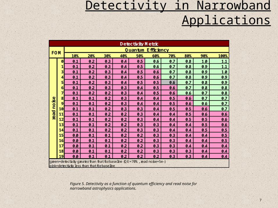
Detectivity in Narrowband Applications

10% 20% 30% 40% 50% 60% 70% 80% 90% 100%0 0.1 0.2 0.3 0.4 0.5 0.6 0.7 0.8 1.0 1.1 1 0.1 0.2 0.3 0.4 0.5 0.6 0.7 0.8 0.9 1.1 3 0.1 0.2 0.3 0.4 0.5 0.6 0.7 0.8 0.9 1.0 4 0.1 0.2 0.3 0.4 0.5 0.6 0.7 0.8 0.9 0.9 5 0.1 0.2 0.3 0.4 0.5 0.5 0.6 0.7 0.8 0.9 6 0.1 0.2 0.3 0.3 0.4 0.5 0.6 0.7 0.8 0.8 7 0.1 0.2 0.2 0.3 0.4 0.5 0.6 0.6 0.7 0.8 8 0.1 0.1 0.2 0.3 0.4 0.4 0.5 0.6 0.7 0.7 9 0.1 0.1 0.2 0.3 0.4 0.4 0.5 0.6 0.6 0.7

10 0.1 0.1 0.2 0.3 0.3 0.4 0.5 0.5 0.6 0.7 11 0.1 0.1 0.2 0.2 0.3 0.4 0.4 0.5 0.6 0.6 12 0.1 0.1 0.2 0.2 0.3 0.4 0.4 0.5 0.5 0.6 13 0.1 0.1 0.2 0.2 0.3 0.3 0.4 0.4 0.5 0.6 14 0.1 0.1 0.2 0.2 0.3 0.3 0.4 0.4 0.5 0.5 15 0.0 0.1 0.1 0.2 0.2 0.3 0.3 0.4 0.4 0.5 16 0.0 0.1 0.1 0.2 0.2 0.3 0.3 0.4 0.4 0.5 17 0.0 0.1 0.1 0.2 0.2 0.3 0.3 0.4 0.4 0.4 18 0.0 0.1 0.1 0.2 0.2 0.3 0.3 0.3 0.4 0.4 19 0.0 0.1 0.1 0.2 0.2 0.2 0.3 0.3 0.4 0.4

read

no

ise


Detectivity Metric


Figure 5. Detectivity as a function of quantum efficiency and read noise for narrowband astrophysics applications.

8

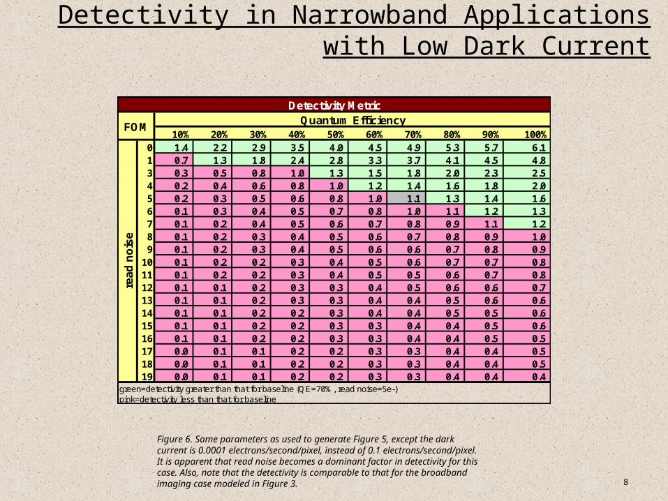
Detectivity in Narrowband Applications with Low Dark Current

10% 20% 30% 40% 50% 60% 70% 80% 90% 100%0 1.4 2.2 2.9 3.5 4.0 4.5 4.9 5.3 5.7 6.1 1 0.7 1.3 1.8 2.4 2.8 3.3 3.7 4.1 4.5 4.8 3 0.3 0.5 0.8 1.0 1.3 1.5 1.8 2.0 2.3 2.5 4 0.2 0.4 0.6 0.8 1.0 1.2 1.4 1.6 1.8 2.0 5 0.2 0.3 0.5 0.6 0.8 1.0 1.1 1.3 1.4 1.6 6 0.1 0.3 0.4 0.5 0.7 0.8 1.0 1.1 1.2 1.3 7 0.1 0.2 0.4 0.5 0.6 0.7 0.8 0.9 1.1 1.2 8 0.1 0.2 0.3 0.4 0.5 0.6 0.7 0.8 0.9 1.0 9 0.1 0.2 0.3 0.4 0.5 0.6 0.6 0.7 0.8 0.9

10 0.1 0.2 0.2 0.3 0.4 0.5 0.6 0.7 0.7 0.8 11 0.1 0.2 0.2 0.3 0.4 0.5 0.5 0.6 0.7 0.8 12 0.1 0.1 0.2 0.3 0.3 0.4 0.5 0.6 0.6 0.7 13 0.1 0.1 0.2 0.3 0.3 0.4 0.4 0.5 0.6 0.6 14 0.1 0.1 0.2 0.2 0.3 0.4 0.4 0.5 0.5 0.6 15 0.1 0.1 0.2 0.2 0.3 0.3 0.4 0.4 0.5 0.6 16 0.1 0.1 0.2 0.2 0.3 0.3 0.4 0.4 0.5 0.5 17 0.0 0.1 0.1 0.2 0.2 0.3 0.3 0.4 0.4 0.5 18 0.0 0.1 0.1 0.2 0.2 0.3 0.3 0.4 0.4 0.5 19 0.0 0.1 0.1 0.2 0.2 0.3 0.3 0.4 0.4 0.4

read

no

ise


Detectivity Metric


Figure 6. Same parameters as used to generate Figure 5, except the dark current is 0.0001 electrons/second/pixel, instead of 0.1 electrons/second/pixel. It is apparent that read noise becomes a dominant factor in detectivity for this case. Also, note that the detectivity is comparable to that for the broadband imaging case modeled in Figure 3.

9

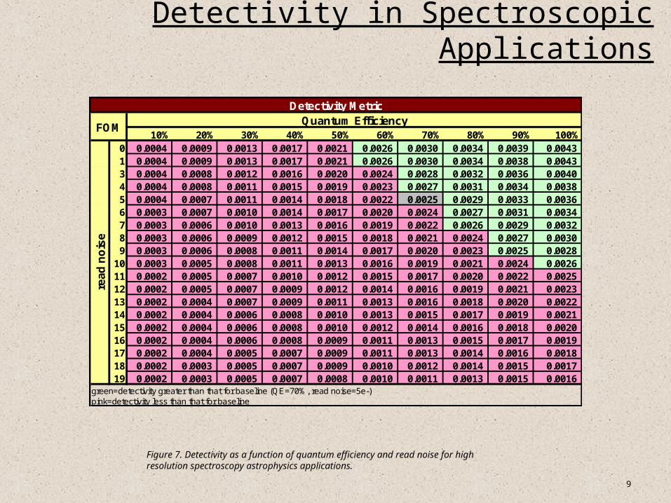
Detectivity in Spectroscopic Applications

10% 20% 30% 40% 50% 60% 70% 80% 90% 100%0 0.0004 0.0009 0.0013 0.0017 0.0021 0.0026 0.0030 0.0034 0.0039 0.0043 1 0.0004 0.0009 0.0013 0.0017 0.0021 0.0026 0.0030 0.0034 0.0038 0.0043 3 0.0004 0.0008 0.0012 0.0016 0.0020 0.0024 0.0028 0.0032 0.0036 0.0040 4 0.0004 0.0008 0.0011 0.0015 0.0019 0.0023 0.0027 0.0031 0.0034 0.0038 5 0.0004 0.0007 0.0011 0.0014 0.0018 0.0022 0.0025 0.0029 0.0033 0.0036 6 0.0003 0.0007 0.0010 0.0014 0.0017 0.0020 0.0024 0.0027 0.0031 0.0034 7 0.0003 0.0006 0.0010 0.0013 0.0016 0.0019 0.0022 0.0026 0.0029 0.0032 8 0.0003 0.0006 0.0009 0.0012 0.0015 0.0018 0.0021 0.0024 0.0027 0.0030 9 0.0003 0.0006 0.0008 0.0011 0.0014 0.0017 0.0020 0.0023 0.0025 0.0028

10 0.0003 0.0005 0.0008 0.0011 0.0013 0.0016 0.0019 0.0021 0.0024 0.0026 11 0.0002 0.0005 0.0007 0.0010 0.0012 0.0015 0.0017 0.0020 0.0022 0.0025 12 0.0002 0.0005 0.0007 0.0009 0.0012 0.0014 0.0016 0.0019 0.0021 0.0023 13 0.0002 0.0004 0.0007 0.0009 0.0011 0.0013 0.0016 0.0018 0.0020 0.0022 14 0.0002 0.0004 0.0006 0.0008 0.0010 0.0013 0.0015 0.0017 0.0019 0.0021 15 0.0002 0.0004 0.0006 0.0008 0.0010 0.0012 0.0014 0.0016 0.0018 0.0020 16 0.0002 0.0004 0.0006 0.0008 0.0009 0.0011 0.0013 0.0015 0.0017 0.0019 17 0.0002 0.0004 0.0005 0.0007 0.0009 0.0011 0.0013 0.0014 0.0016 0.0018 18 0.0002 0.0003 0.0005 0.0007 0.0009 0.0010 0.0012 0.0014 0.0015 0.0017 19 0.0002 0.0003 0.0005 0.0007 0.0008 0.0010 0.0011 0.0013 0.0015 0.0016

read

no

ise


Detectivity Metric


Figure 7. Detectivity as a function of quantum efficiency and read noise for high resolution spectroscopy astrophysics applications.

10

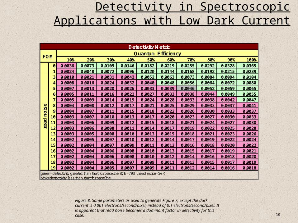
Detectivity in Spectroscopic Applications with Low Dark Current

10% 20% 30% 40% 50% 60% 70% 80% 90% 100%0 0.0036 0.0073 0.0109 0.0146 0.0182 0.0219 0.0255 0.0292 0.0328 0.0365 1 0.0024 0.0048 0.0072 0.0096 0.0120 0.0144 0.0168 0.0192 0.0215 0.0239 3 0.0010 0.0021 0.0031 0.0042 0.0052 0.0063 0.0073 0.0084 0.0094 0.0104 4 0.0008 0.0016 0.0024 0.0032 0.0040 0.0048 0.0056 0.0064 0.0072 0.0080 5 0.0007 0.0013 0.0020 0.0026 0.0033 0.0039 0.0046 0.0052 0.0059 0.0065 6 0.0005 0.0011 0.0016 0.0022 0.0027 0.0033 0.0038 0.0044 0.0049 0.0055 7 0.0005 0.0009 0.0014 0.0019 0.0024 0.0028 0.0033 0.0038 0.0042 0.0047 8 0.0004 0.0008 0.0012 0.0017 0.0021 0.0025 0.0029 0.0033 0.0037 0.0041 9 0.0004 0.0007 0.0011 0.0015 0.0018 0.0022 0.0026 0.0030 0.0033 0.0037

10 0.0003 0.0007 0.0010 0.0013 0.0017 0.0020 0.0023 0.0027 0.0030 0.0033 11 0.0003 0.0006 0.0009 0.0012 0.0015 0.0018 0.0021 0.0024 0.0027 0.0030 12 0.0003 0.0006 0.0008 0.0011 0.0014 0.0017 0.0019 0.0022 0.0025 0.0028 13 0.0003 0.0005 0.0008 0.0010 0.0013 0.0015 0.0018 0.0021 0.0023 0.0026 14 0.0002 0.0005 0.0007 0.0010 0.0012 0.0014 0.0017 0.0019 0.0022 0.0024 15 0.0002 0.0004 0.0007 0.0009 0.0011 0.0013 0.0016 0.0018 0.0020 0.0022 16 0.0002 0.0004 0.0006 0.0008 0.0010 0.0013 0.0015 0.0017 0.0019 0.0021 17 0.0002 0.0004 0.0006 0.0008 0.0010 0.0012 0.0014 0.0016 0.0018 0.0020 18 0.0002 0.0004 0.0006 0.0007 0.0009 0.0011 0.0013 0.0015 0.0017 0.0019 19 0.0002 0.0004 0.0005 0.0007 0.0009 0.0011 0.0012 0.0014 0.0016 0.0018

read

no

ise


Detectivity Metric


Figure 8. Same parameters as used to generate Figure 7, except the dark current is 0.001 electrons/second/pixel, instead of 0.1 electrons/second/pixel. It is apparent that read noise becomes a dominant factor in detectivity for this case.

11

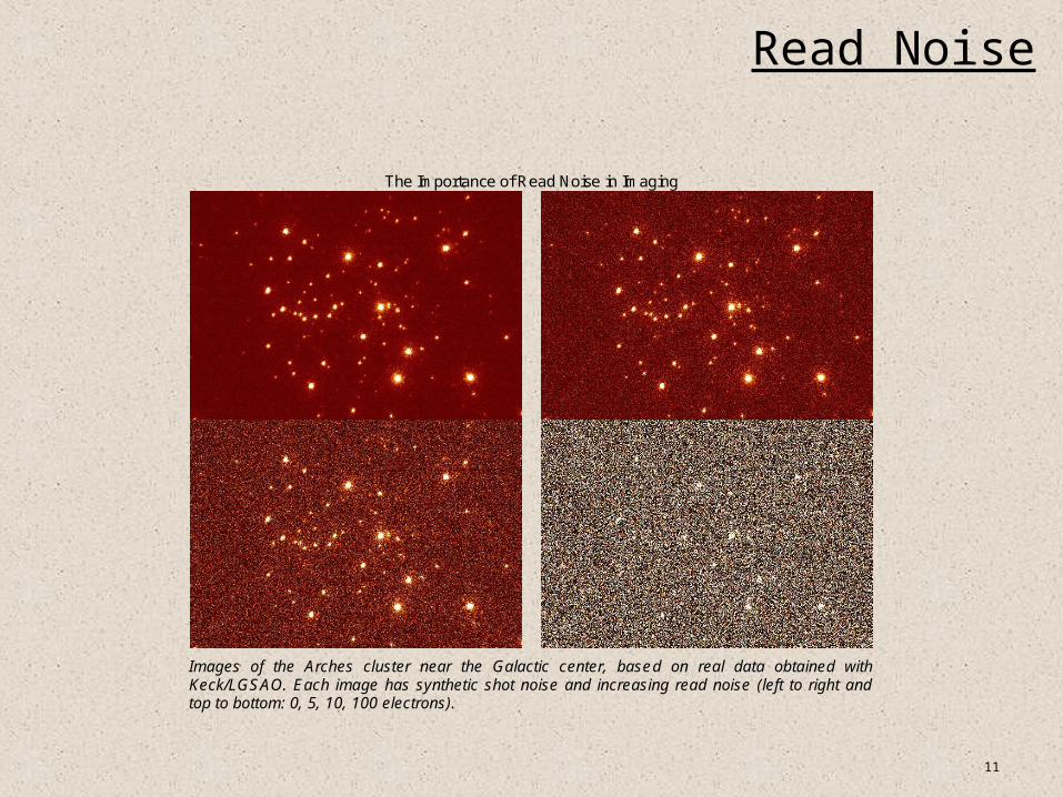
Read Noise

The Importance of Read Noise in Imaging

Images of the Arches cluster near the Galactic center, based on real data obtained with Keck/LGSAO. Each image has synthetic shot noise and increasing read noise (left to right and top to bottom: 0, 5, 10, 100 electrons).

12

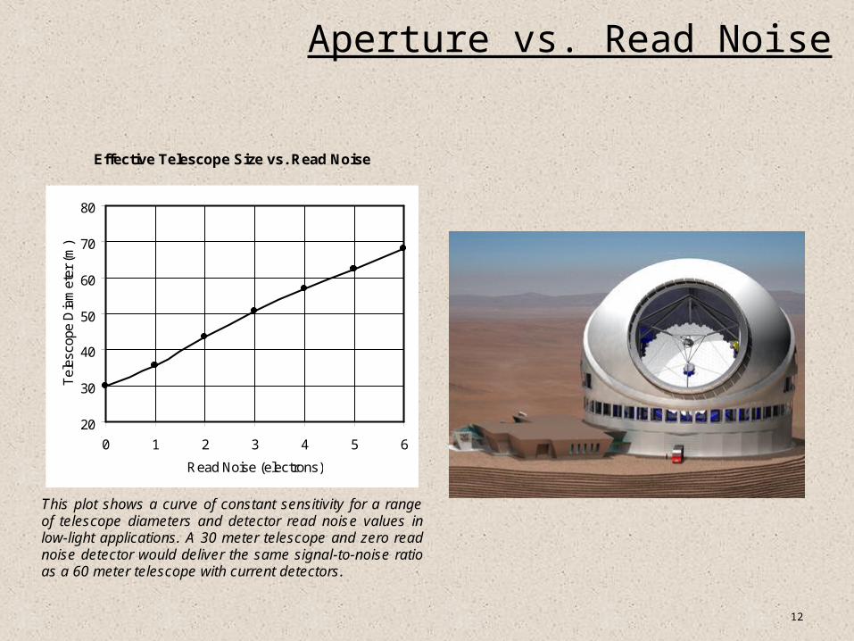
Aperture vs. Read Noise

Effective Telescope Size vs. Read Noise

20

30

40

50

60

70

80

0 1 2 3 4 5 6

Read Noise (electrons)

Tel

esco

pe D

iam

eter

(m

)

This plot shows a curve of constant sensitivity for a range of telescope diameters and detector read noise values in low-light applications. A 30 meter telescope and zero read noise detector would deliver the same signal-to-noise ratio as a 60 meter telescope with current detectors.

13

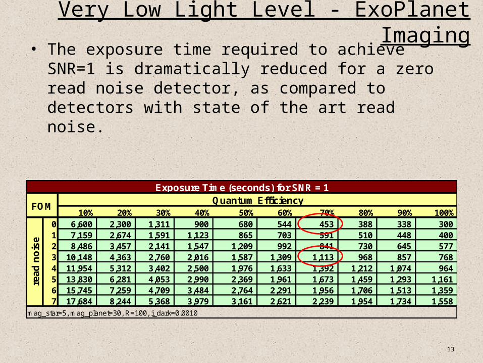
Very Low Light Level - ExoPlanet Imaging• The exposure time required to achieve SNR=1 is dramatically

reduced for a zero read noise detector, as compared to detectors with state of the art read noise.

10% 20% 30% 40% 50% 60% 70% 80% 90% 100%0 6,600 2,300 1,311 900 680 544 453 388 338 300 1 7,159 2,674 1,591 1,123 865 703 591 510 448 400 2 8,486 3,457 2,141 1,547 1,209 992 841 730 645 577 3 10,148 4,363 2,760 2,016 1,587 1,309 1,113 968 857 768 4 11,954 5,312 3,402 2,500 1,976 1,633 1,392 1,212 1,074 964 5 13,830 6,281 4,053 2,990 2,369 1,961 1,673 1,459 1,293 1,161 6 15,745 7,259 4,709 3,484 2,764 2,291 1,956 1,706 1,513 1,359 7 17,684 8,244 5,368 3,979 3,161 2,621 2,239 1,954 1,734 1,558

rea

d n

ois

e

mag_star=5, mag_planet=30, R=100, i_dark=0.0010

Exposure Time (seconds) for SNR = 1


14

Principles of Quantum Limited Detectors

15

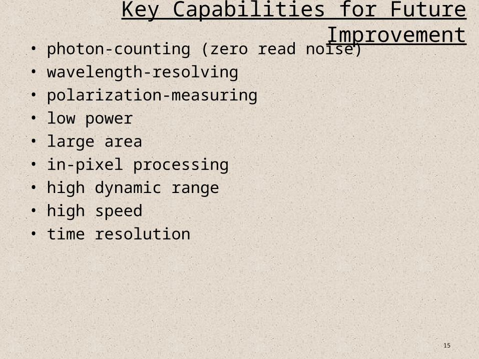
Key Capabilities for Future Improvement• photon-counting (zero read noise)

• wavelength-resolving

• polarization-measuring

• low power

• large area

• in-pixel processing

• high dynamic range

• high speed

• time resolution

16

QLID Technology Contenders

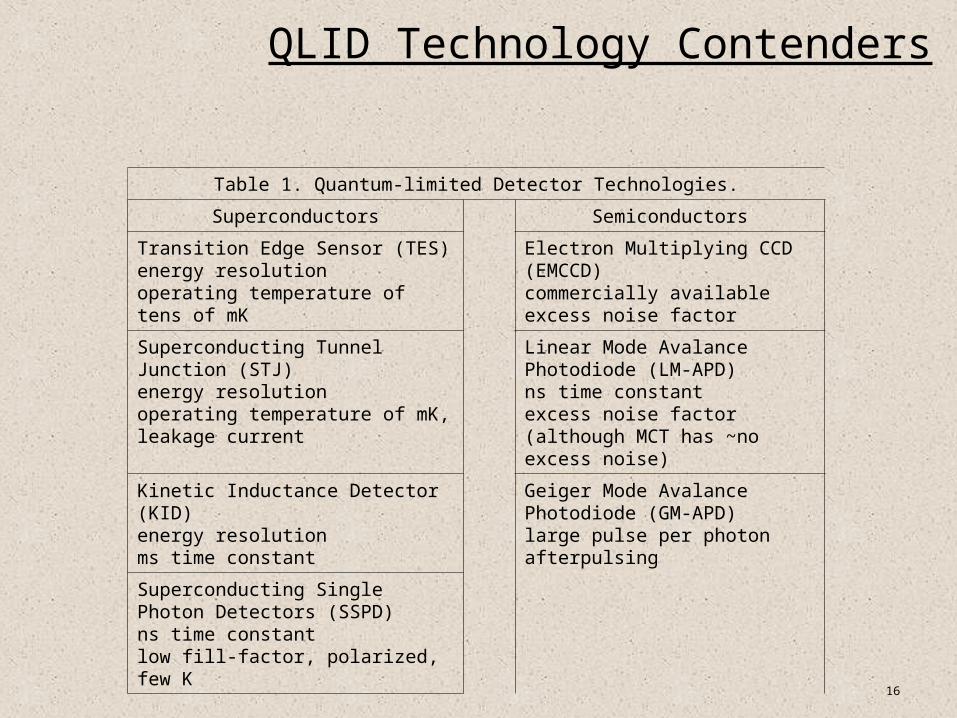
Table 1. Quantum-limited Detector Technologies.

Superconductors Semiconductors

Transition Edge Sensor (TES)energy resolutionoperating temperature of tens of mK

Electron Multiplying CCD (EMCCD)commercially availableexcess noise factor

Superconducting Tunnel Junction (STJ)energy resolutionoperating temperature of mK, leakage current

Linear Mode Avalance Photodiode (LM-APD)ns time constantexcess noise factor (although MCT has ~no excess noise)

Kinetic Inductance Detector (KID)energy resolutionms time constant

Geiger Mode Avalance Photodiode (GM-APD)large pulse per photonafterpulsingSuperconducting Single Photon Detectors

(SSPD)ns time constantlow fill-factor, polarized, few K

17

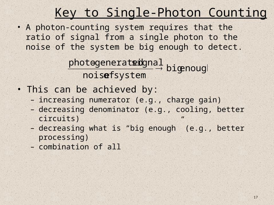
Key to Single-Photon Counting• A photon-counting system requires that the ratio of signal

from a single photon to the noise of the system be big enough to detect.

enough bigsystem of noise

signal generated-photo

• This can be achieved by:– increasing numerator (e.g., charge gain)– decreasing denominator (e.g., cooling, better circuits)– decreasing what is “big enough” (e.g., better processing)– combination of all

18

Superconductors• Most metals have descreased resistance with lower

temperature, but they still have finite resistance at T=0 K.

• Superconductors lose all resistance to electrical current at some temperature, Tc. Examples include: Pb, Al, Sn, and Nb.

• Electrons in superconductors bond as “Cooper pairs” that do not interact with the ion lattice below Tc because the required interaction energy exceeds the thermal energy in the crystal.

• In general, Tc<4.2 K.

• Recent developments have produced “high” temperature superconductors, for which Tc>77 K (temperature of liquid nitrogen).

19

Slide Title

20

Avalanche Photodiodes (APDs)

21

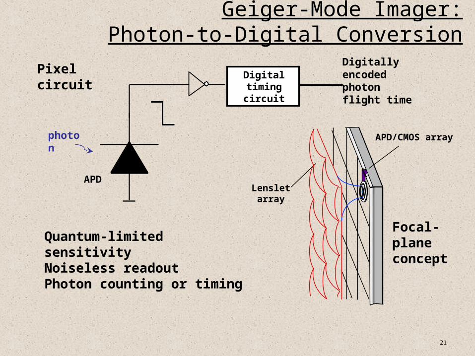
Geiger-Mode Imager:Photon-to-Digital Conversion

Quantum-limited sensitivityNoiseless readout Photon counting or timing

APD

Digitaltimingcircuit

Digitallyencodedphotonflight time

photon

Lensletarray

APD/CMOS array

Focal-plane concept

Pixel circuit

22

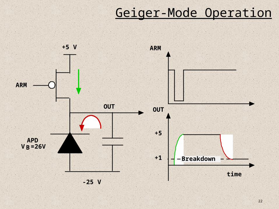
Geiger-Mode Operation

-25 V

+5 V

ARM

+5

+1 Breakdown

ARM

OUT OUT

time

APD VB=26V

23

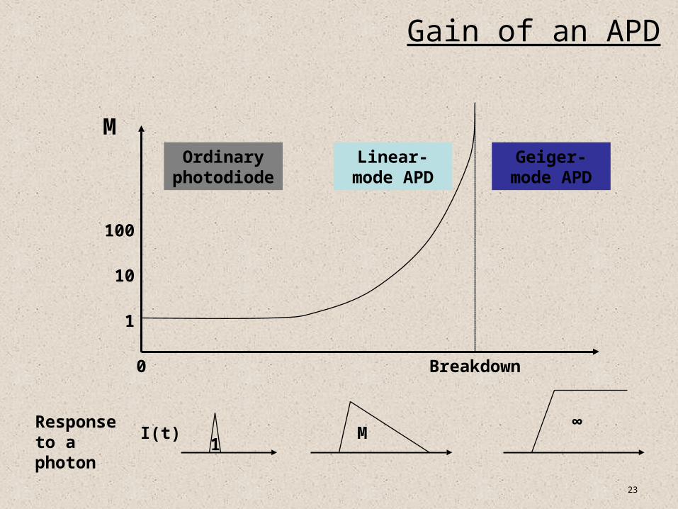
Gain of an APD

1

10

100

M

Breakdown0

Ordinary photodiode

Linear-mode APD

Geiger-mode APD

Response to a photon M

1∞

I(t)

24

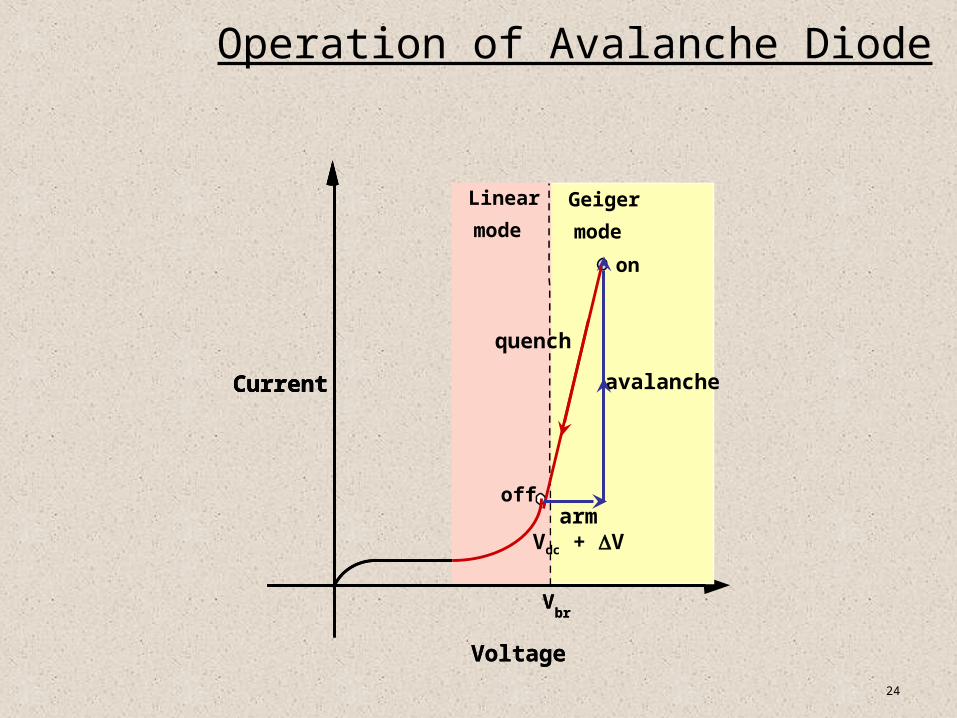
Current

Voltage

Current

Linear

mode

Geiger

mode

Vbr

on

off

Current

Voltage

Current

Linear

mode

Geiger

mode

Vbr

on

avalanche

off

quench

armVdc + V

Operation of Avalanche Diode

25

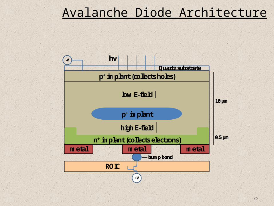
Avalanche Diode Architecture

10 µm

0.5 µm

metal metal

p+ implant (collects holes)

p+ implant

n+ implant (collects electrons)

low E-field

high E-field

-V hν

ROIC

metalbump bond

Quartz substrate

+V

10 µm

0.5 µm

metal metal

p+ implant (collects holes)

p+ implant

n+ implant (collects electrons)

low E-field

high E-field

-V hν

ROIC

metalbump bond

Quartz substrate

+V

26

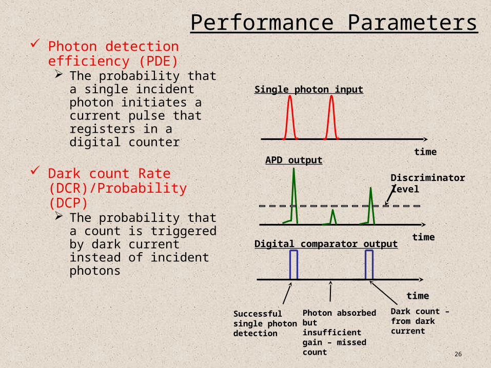
Performance Parameters Photon detection efficiency

(PDE) The probability that a single

incident photon initiates a current pulse that registers in a digital counter

Dark count Rate (DCR)/Probability (DCP) The probability that a count is

triggered by dark current instead of incident photons

timetime

timetime

time

Single photon input

APD output

Discriminatorlevel

Digital comparator output

Successfulsingle photondetection

Photon absorbed but insufficient gain – missed count

Dark count – from dark current

27

APD Charge Gain• Show animation with thumping euro-techno disco music

http://techresearch.intel.com/spaw2/uploads/files/SiliconPhotonics.html

http://techresearch.intel.com/spaw2/uploads/files/SiliconPhotonics.html

28

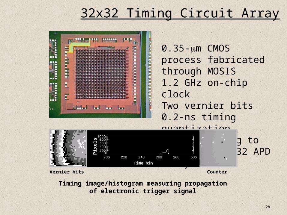
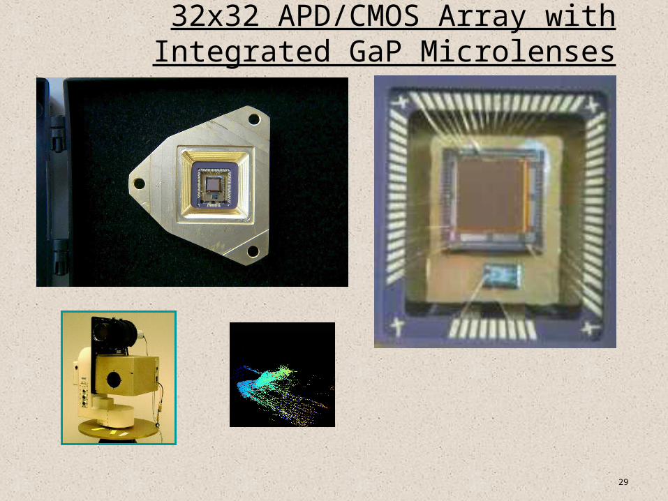
32x32 Timing Circuit Array

0.35-m CMOS process fabricated through MOSIS1.2 GHz on-chip clockTwo vernier bits0.2-ns timing quantization100-m spacing to match the 32x32 APD array

Timing image/histogram measuring propagation of electronic trigger signal

Vernier bits Counter

Time bin

Pix

els

29

32x32 APD/CMOS Array with Integrated GaP Microlenses

30

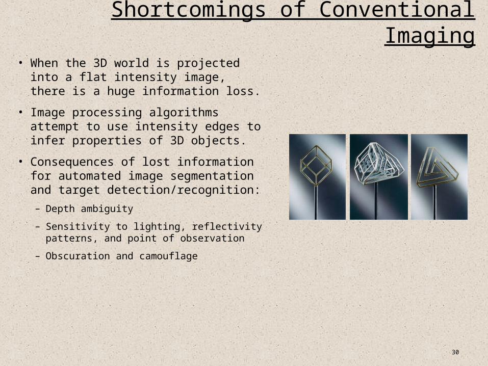
Shortcomings of Conventional Imaging

• When the 3D world is projected into a flat intensity image, there is a huge information loss.

• Image processing algorithms attempt to use intensity edges to infer properties of 3D objects.

• Consequences of lost information for automated image segmentation and target detection/recognition:

– Depth ambiguity

– Sensitivity to lighting, reflectivity patterns, and point of observation

– Obscuration and camouflage

31

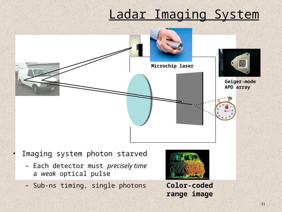
Ladar Imaging System

• Imaging system photon starved

– Each detector must precisely time a weak optical pulse

– Sub-ns timing, single photons

Microchip laser

Geiger-mode APD array

Color-codedrange image

32

Laser Radar Brassboard System (Gen I)

• 4 4 APD array• External rack-mounted timing circuits

• Doubled Nd:YAG passively Q-switched microchip laser

(produces 30 µJ, 250 ps pulses at = 532 nm)

• Transmit/receive field of view scanned to generate 128 128 images

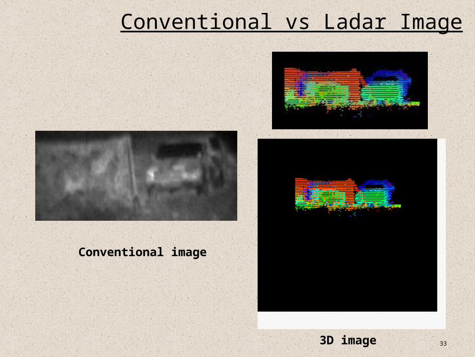
Taken at noontime on a sunny day

33

Conventional vs Ladar Image

Conventional image

3D image

34

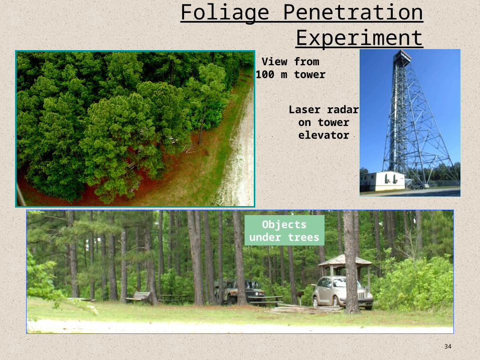
Foliage Penetration Experiment

Laser radar on tower elevator

View from100 m tower

Objectsunder trees

35

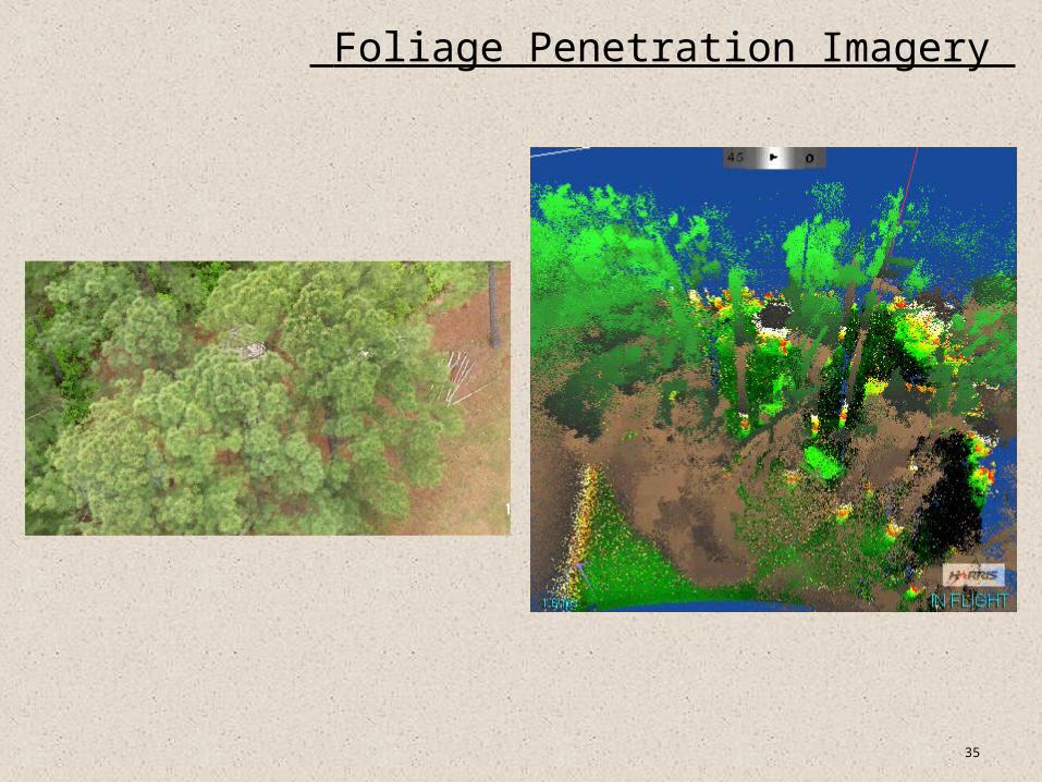
Foliage Penetration Imagery

36

Transition Edge Sensors (TESs)

37

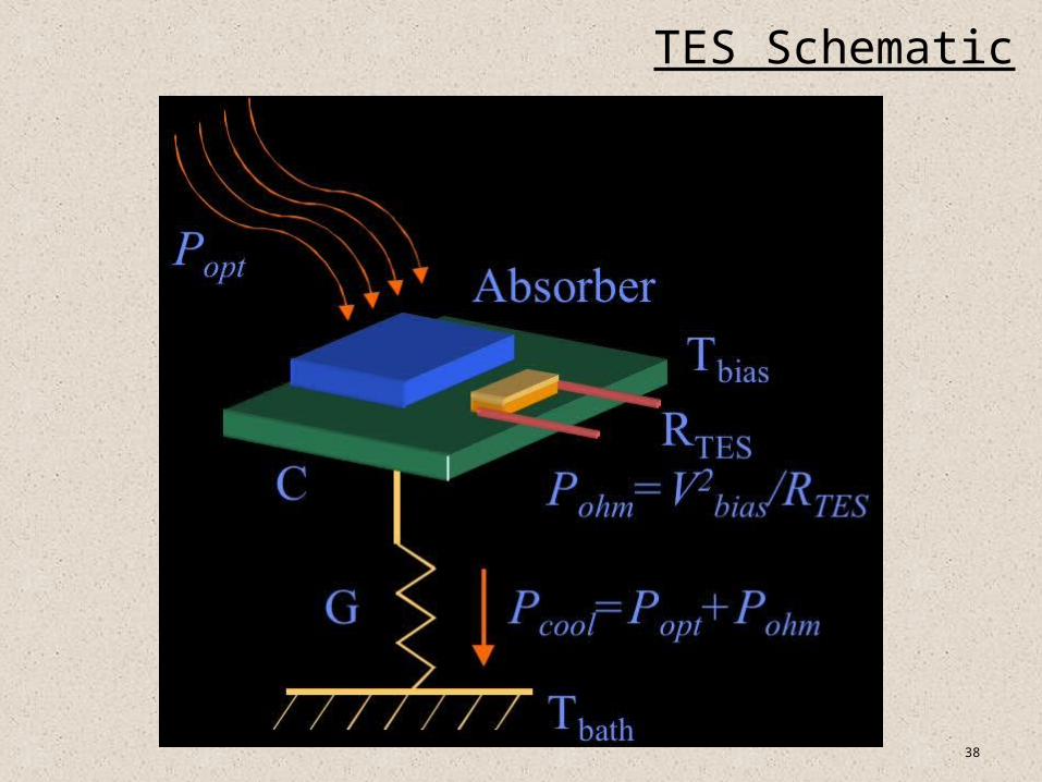
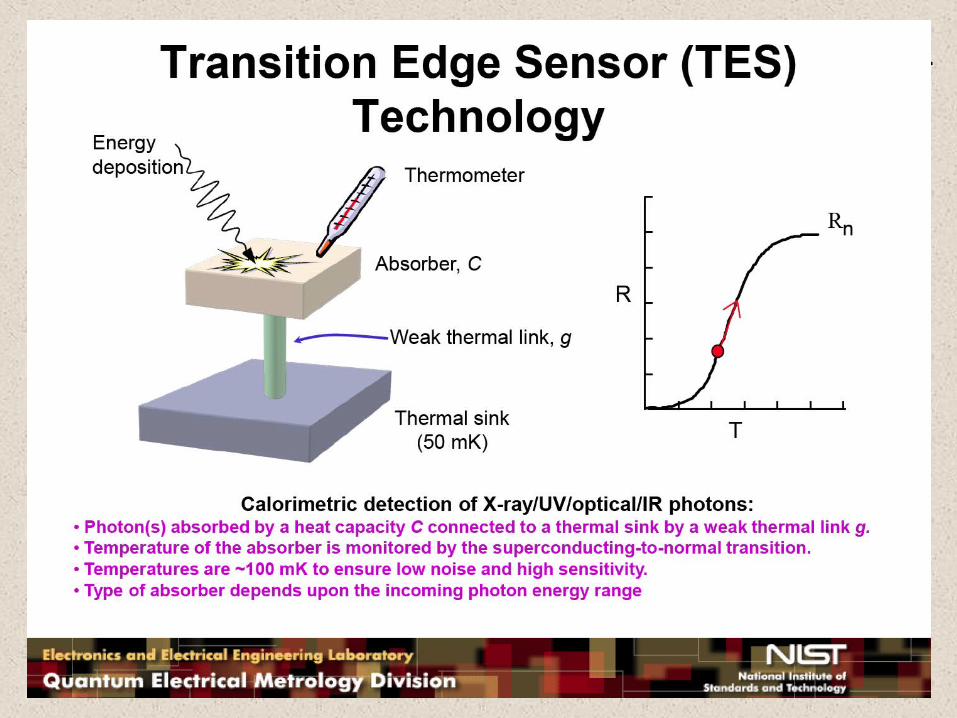
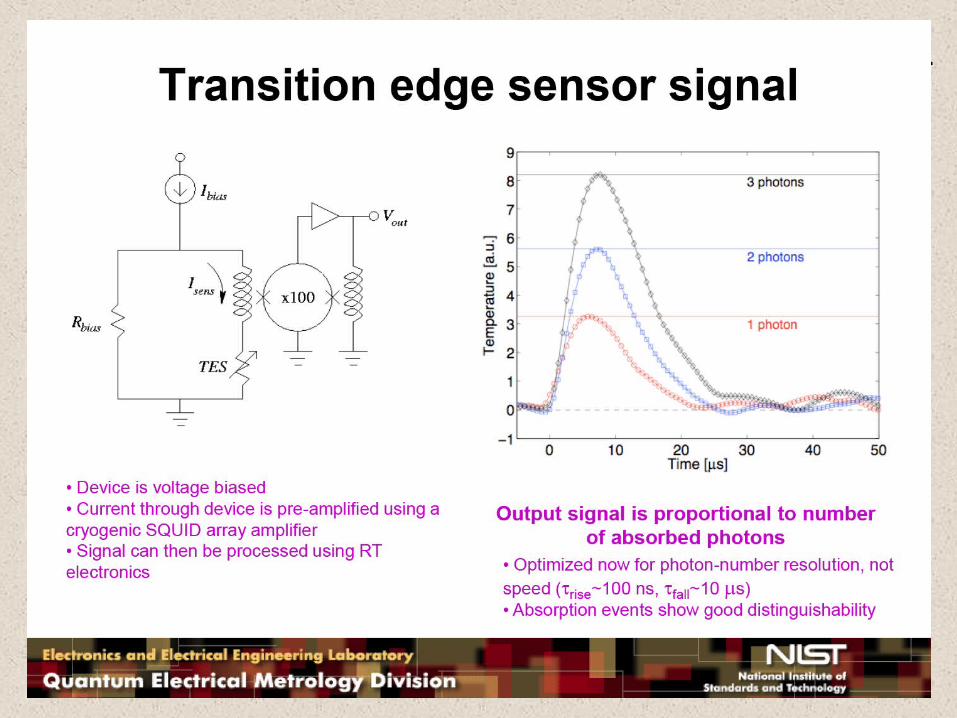
Transition Edge Sensors (TES)• A TES is similar to a bolometer, in that photon energy is

detected when it is absorbed in a material that changes resistance with temperature.

• The difference is that a TES is held at a temperature just below the transition temperature at which the material becomes supconducting.

• The effective change in resistance when photons are absorbed is very large (and easy to detect).

• One of the disadvantages of using TES’s is that the transition temperature is usually very low, requiring exotic cooling techniques.

38

TES Schematic

39

Slide Title• xxxxxx

40

TES Wavelength Resolution

41

Slide Title

42

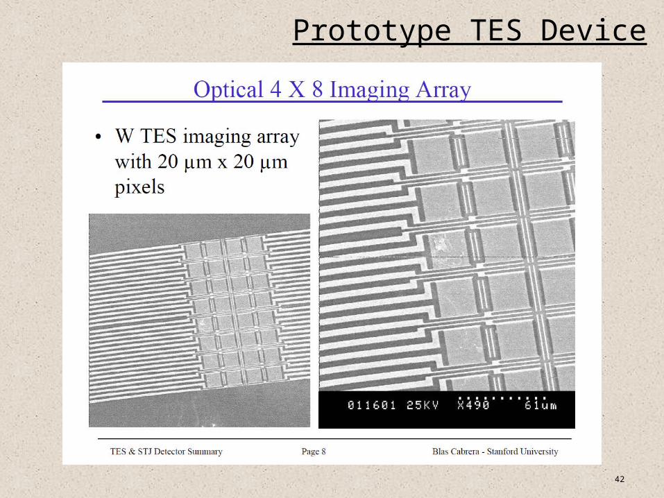
Prototype TES Device

43

Superconducting Tunneling Junctions (STJs)

44

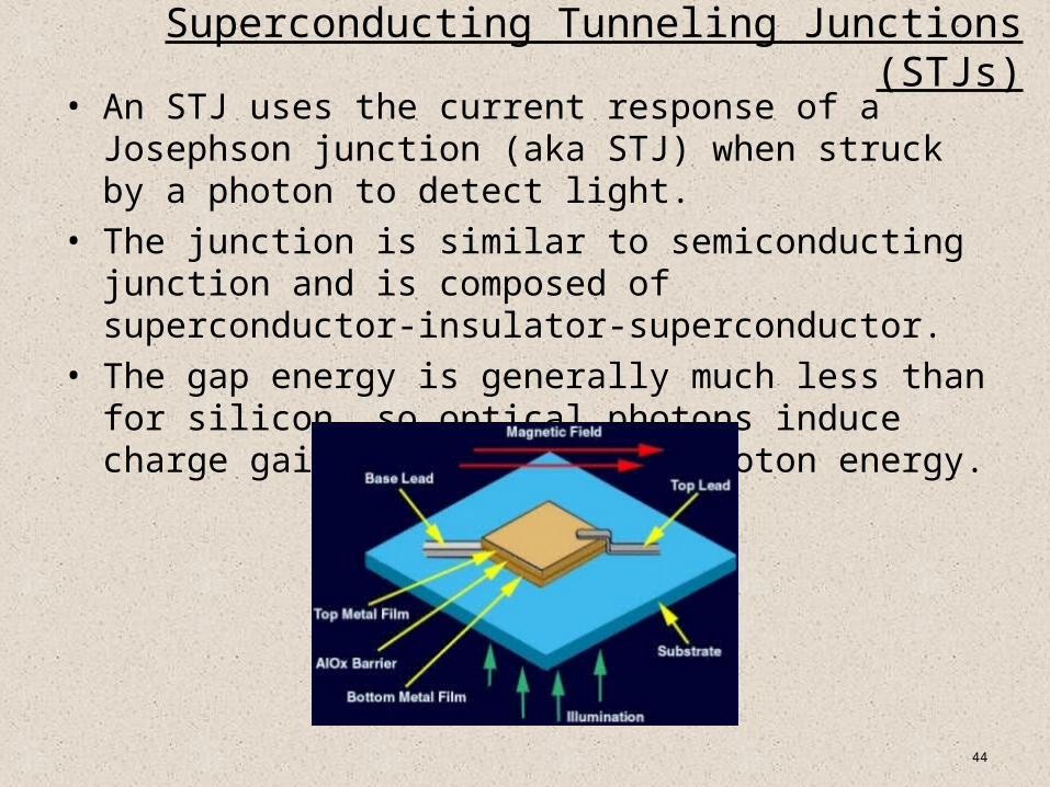
Superconducting Tunneling Junctions (STJs)• An STJ uses the current response of a Josephson junction (aka

STJ) when struck by a photon to detect light.

• The junction is similar to semiconducting junction and is composed of superconductor-insulator-superconductor.

• The gap energy is generally much less than for silicon, so optical photons induce charge gain that depends on photon energy.

45

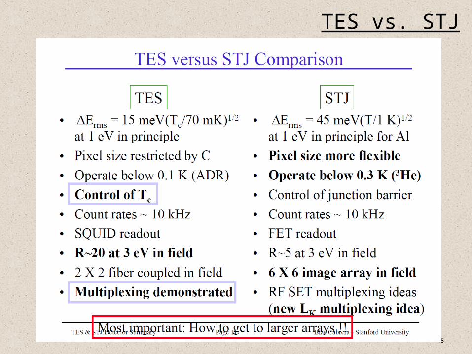
TES vs. STJ

46

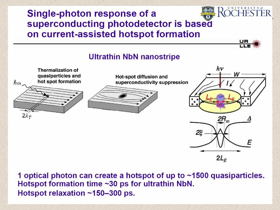
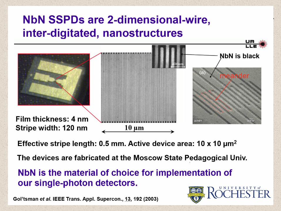
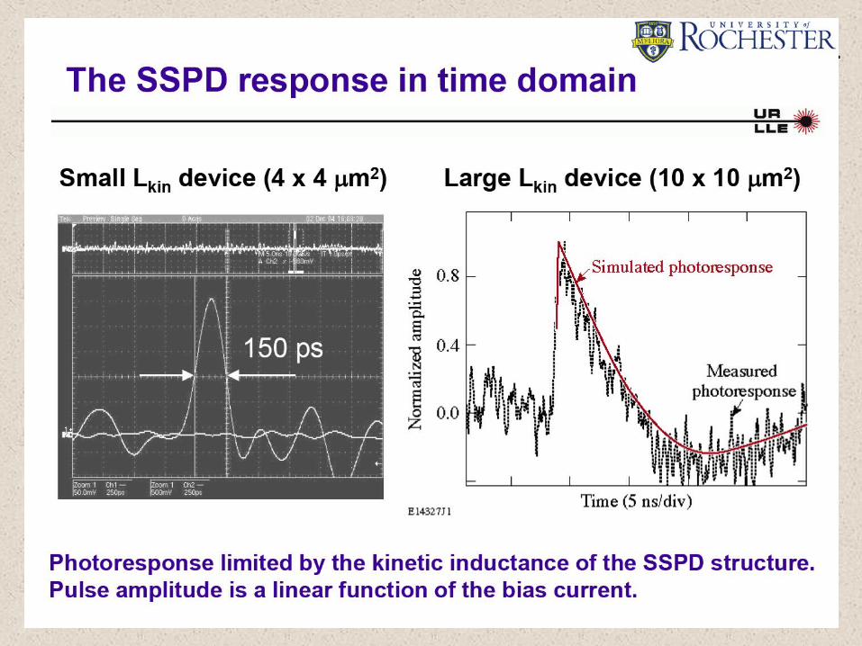
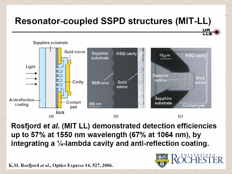
Superconducting Single Photon Detectors (SSPDs)

47

Slide Title

48

Slide Title

49

Slide Title

50

Slide Title

51

Slide Title

52

Slide Title• xxxxxx

53

Slide Title

Documents

Astronomical Observational Techniques and Instrumentation