Astron. Astrophys. 351, 1139–1148 (1999) ASTRONOMYAND

ASTROPHYSICS

Temporal variability in the electron densityat the solar transition region

M.E. Perez1, J.G. Doyle1, E. O’Shea2, and F.P. Keenan2

1 Armagh Observatory, College Hill, Armagh BT61 9DG, Ireland (epp,jgd@star.arm.ac.uk)2 Department of Pure and Applied Physics, Queen’s University Belfast, Belfast BT7 1NN, Ireland (E.Oshea,F.Keenan@qub.ac.uk)

Received 23 July 1999 / Accepted 6 October 1999

Abstract. The electron density as measured in the transitionregion of a coronal hole, a ‘quiet’ Sun region at disk center plusan active region shows variations of up to a factor of two atTe ∼ 1.5 105 K, lasting at most only a few minutes. There isremarkable agreement between the number of such variations,their temporal variability and duration in the coronal hole and‘quiet’ Sun datasets, consistent with an earlier bright point study.There appears to be evidence of super-granular cells, with the in-creases in electron density occurring along the network bound-aries. At some locations, periodicities of between 8 and 16 minare visible in the electron density variations. We associate thesevariations with the sites of explosive events.

Key words: line: profiles – Sun: activity – Sun: corona – Sun:transition region – Sun: UV radiation

1. Introduction

There are abundant references to solar electron density (Ne)diagnostics in the literature, with e.g. emission lines arisingfrom transitions in Oivproviding accurate determinations of Ne

(Griffiths et al. 1999, Doschek et al. 1998, O’Shea et al. 1998,Spadaro et al. 1994, Dwivedi & Gupta 1991, Hayes & Shine1987, Feldman & Doschek 1978). For instance, Hayes & Shine(1987) used the ratio of Siiv 1402.8A and Oiv 1401.2A, andfound that short-lived bursts typically showed electron densityincreases coupled with a small line shift to the red. They sug-gested this might be caused by ‘ micro-flares ’. Cheng (1980),analysing coronal loops in Fexv & Fexvi lines, found a den-sity enhancement of∼ 30% in a loop within 7 minutes, plus aslower variation over a longer time interval. He suggested thatthis increase in density could be due to mass ejection from lowerregions, and the associated dissipation of the electric currentassociated with the resulting high-density twisted flux strands(Nakagawa & Stenflo 1979) contributing to the coronal heating.

In this paper we use the Oiv 2s22p2P o → 2s2p4P density-sensitive multiplet around 1400A to analyse time-series solarspectra. More precisely, we use the Oiv 1399.8A and 1401.2Alines for our analysis.

Send offprint requests to: M.E. Perez

The Solar Ultraviolet Measurements of Emitted Radiation(SUMER) instrument (Wilhelm et al. 1997) onSOHOprovidesthe opportunity to observe the solar atmosphere in the spectralrange from∼500 to 1600A with high spectral and spatial res-olution. In first order, the spectral resolution is∼43mA, while∼22mA is achieved in second order. The spatial resolution is ap-proximately 1 arc sec in the E-W direction and 2 arc sec along theslit (N-S direction). It should be pointed out that only lines sep-arated by less than 40A in first order, and 20A in second order,can be observed simultaneously with SUMER due to the size ofthe CCD. Surprisingly few lines can be used for density diag-nostics, due to blending problems, the weakness of some lines,and the fact that possible useful lines cannot be observed simul-taneously. The line pair most useful for diagnosing the transitionregion is probably Oiv 1399.8/1401.2 (Wikstol et al. 1997).

2. Theoretical line ratios

The model ion for Oiv consisted of the 8 energetically lowestLS states, namely 2s22p 2P; 2s2p2 4P, 2D, 2S, 2P; 2p3 4S, 2Dand2P, making a total of 15 fine-structure levels. Energies forall of these were obtained from Safronova et al. (1996).

Electron impact excitation rates for transitions in Oiv weretaken from Zhang et al. (1994). For Einstein A-coefficients, thecalculations of Nussbaumer & Storey (1982), Brage et al. (1996)and Dankworth & Trefftz (1978) were adopted for the 2s22p2P1/2 – 2s22p 2P3/2, 2s22p – 2s2p2 and 2s2p2 – 2p3 transitions,respectively. As noted by, for example Seaton (1964), excitationby protons may be important for fine-structure transitions. Inthe present analysis we have used the proton rates of Foster etal. (1996, 1997) for transitions within 2s22p 2P and 2s2p2 4P,respectively.

Using the atomic data discussed above in conjunction withthe statistical equilibrium code of Dufton (1977), relative Oivlevel populations and hence emission line strengths were calcu-lated for a range of electron temperatures and densities. Detailsof the procedures involved and approximations made may befound in Dufton (1977) and Dufton et al. (1978).

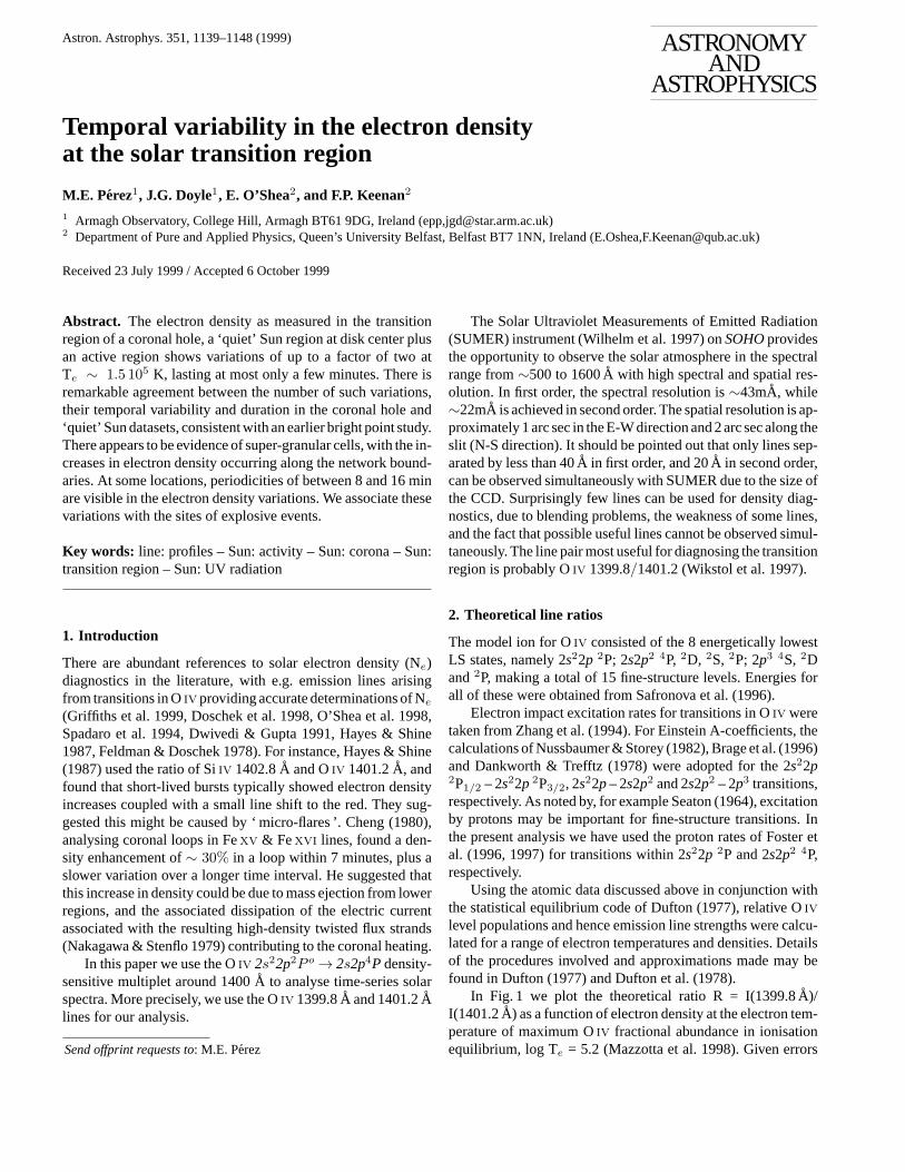
In Fig. 1 we plot the theoretical ratio R = I(1399.8A)/I(1401.2A) as a function of electron density at the electron tem-perature of maximum Oiv fractional abundance in ionisationequilibrium, log Te = 5.2 (Mazzotta et al. 1998). Given errors

1140 M.E. Perez et al.: Temporal variability in the electron density at the solar transition region

Table 1.Description of observational data

Date 10 July 1996 14 July 1996

Start UT 07:36:15 17:09:42 22:32:46 01:07:23End UT 08:42:56 18:16:42 00:00:09 02:14:04Pointing: X,Y (630,-200) (3,0) (3,0) (0,910)Slit 〈n〉 (arc sec2) 〈6〉 0.3 × 120 〈4〉 1.0 × 120 〈4〉 1.0 × 120 〈4〉 1.0 × 120Location AR QS QS Northern CHX Width/Y Width ∼7 × 82 ∼10 × 112 ∼10 × 85 ∼1 × 112Exposure time 20 s 20 s 20 s 20 s

Fig. 1.Theoretical Oiv I(1399.8A)/I(1401.2A) line ratios, calculatedat an electron temperature of log Te = 5.2. The present results are shownwith a continuous line, and those from the CHIANTI database with adashed line.

of typically ±10% in the adopted atomic data (see referencesabove), we would expect the theoretical values of R to be ac-curate to better than±15%. We note that R is very insensitiveto variations in the adopted electron temperature. For example,varying Te by 0.2 dex leads to a<1% change in the theoreticalR ratio.

Also shown for comparison in Fig. 1 are the values of Robtained from the CHIANTI database (Landi et al. 1999). Aninspection of the figure shows that the current diagnostic calcu-lations are quite similar to those from CHIANTI. We thereforeadopt the former in the present analysis, but note that use of theCHIANTI ratios would not significantly affect our results nordiscussion.

3. SUMER observations and data reduction

3.1. Data

The data used here were obtained with SUMER on-boardSOHOon 10 and 14 July 1996 (see Table 1). These datasets were takenin order to look for variations in electron density in the solartransition region, using the density sensitive line ratio of Oiv1399/1401. The pointing for our observations were centered ondifferent regions in the Sun: one extended active region (AR),two ‘quiet’ Sun regions (henceforth QS1 and QS2) and one

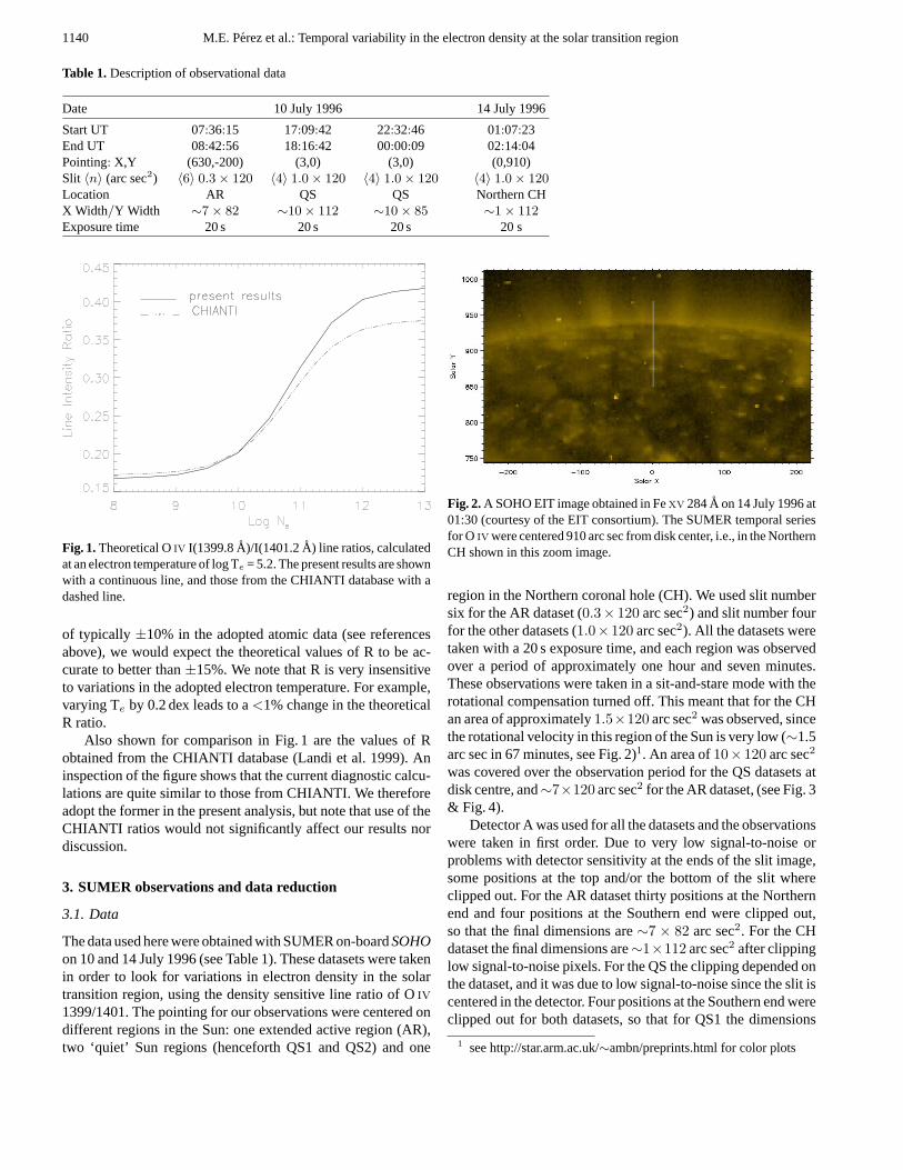
Fig. 2.A SOHO EIT image obtained in Fexv 284A on 14 July 1996 at01:30 (courtesy of the EIT consortium). The SUMER temporal seriesfor O iv were centered 910 arc sec from disk center, i.e., in the NorthernCH shown in this zoom image.

region in the Northern coronal hole (CH). We used slit numbersix for the AR dataset (0.3× 120 arc sec2) and slit number fourfor the other datasets (1.0×120 arc sec2). All the datasets weretaken with a 20 s exposure time, and each region was observedover a period of approximately one hour and seven minutes.These observations were taken in a sit-and-stare mode with therotational compensation turned off. This meant that for the CHan area of approximately1.5×120 arc sec2 was observed, sincethe rotational velocity in this region of the Sun is very low (∼1.5arc sec in 67 minutes, see Fig. 2)1. An area of10× 120 arc sec2

was covered over the observation period for the QS datasets atdisk centre, and∼7×120 arc sec2 for the AR dataset, (see Fig. 3& Fig. 4).

Detector A was used for all the datasets and the observationswere taken in first order. Due to very low signal-to-noise orproblems with detector sensitivity at the ends of the slit image,some positions at the top and/or the bottom of the slit whereclipped out. For the AR dataset thirty positions at the Northernend and four positions at the Southern end were clipped out,so that the final dimensions are∼7 × 82 arc sec2. For the CHdataset the final dimensions are∼1×112 arc sec2 after clippinglow signal-to-noise pixels. For the QS the clipping depended onthe dataset, and it was due to low signal-to-noise since the slit iscentered in the detector. Four positions at the Southern end wereclipped out for both datasets, so that for QS1 the dimensions

1 see http://star.arm.ac.uk/∼ambn/preprints.html for color plots

M.E. Perez et al.: Temporal variability in the electron density at the solar transition region 1141

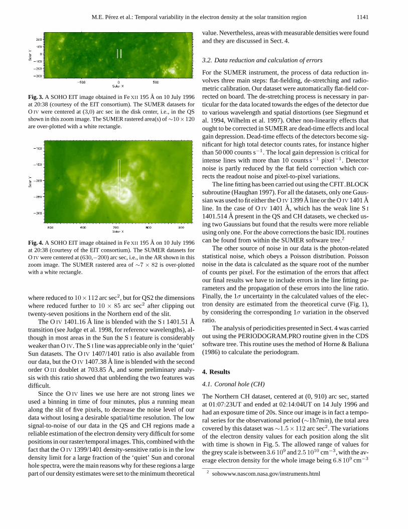
Fig. 3. A SOHO EIT image obtained in Fexii 195A on 10 July 1996at 20:38 (courtesy of the EIT consortium). The SUMER datasets forO iv were centered at (3,0) arc sec in the disk center, i.e., in the QSshown in this zoom image. The SUMER rastered area(s) of∼10×120are over-plotted with a white rectangle.

Fig. 4. A SOHO EIT image obtained in Fexii 195A on 10 July 1996at 20:38 (courtesy of the EIT consortium). The SUMER datasets forO iv were centered at (630,−200) arc sec, i.e., in the AR shown in thiszoom image. The SUMER rastered area of∼7 × 82 is over-plottedwith a white rectangle.

where reduced to10×112 arc sec2, but for QS2 the dimensionswhere reduced further to10 × 85 arc sec2 after clipping outtwenty-seven positions in the Northern end of the slit.

The Oiv 1401.16A line is blended with the Si 1401.51Atransition (see Judge et al. 1998, for reference wavelengths), al-though in most areas in the Sun the Si feature is considerablyweaker than Oiv. The Si line was appreciable only in the ‘quiet’Sun datasets. The Oiv 1407/1401 ratio is also available fromour data, but the Oiv 1407.38A line is blended with the secondorder Oiii doublet at 703.85A, and some preliminary analy-sis with this ratio showed that unblending the two features wasdifficult.

Since the Oiv lines we use here are not strong lines weused a binning in time of four minutes, plus a running meanalong the slit of five pixels, to decrease the noise level of ourdata without losing a desirable spatial/time resolution. The lowsignal-to-noise of our data in the QS and CH regions made areliable estimation of the electron density very difficult for somepositions in our raster/temporal images. This, combined with thefact that the Oiv 1399/1401 density-sensitive ratio is in the lowdensity limit for a large fraction of the ‘quiet’ Sun and coronalhole spectra, were the main reasons why for these regions a largepart of our density estimates were set to the minimum theoretical

value. Nevertheless, areas with measurable densities were foundand they are discussed in Sect. 4.

3.2. Data reduction and calculation of errors

For the SUMER instrument, the process of data reduction in-volves three main steps: flat-fielding, de-stretching and radio-metric calibration. Our dataset were automatically flat-field cor-rected on board. The de-stretching process is necessary in par-ticular for the data located towards the edges of the detector dueto various wavelength and spatial distortions (see Siegmund etal. 1994, Wilhelm et al. 1997). Other non-linearity effects thatought to be corrected in SUMER are dead-time effects and localgain depression. Dead-time effects of the detectors become sig-nificant for high total detector counts rates, for instance higherthan 50 000 counts s−1. The local gain depression is critical forintense lines with more than 10 counts s−1 pixel−1. Detectornoise is partly reduced by the flat field correction which cor-rects the readout noise and pixel-to-pixel variations.

The line fitting has been carried out using the CFITBLOCKsubroutine (Haughan 1997). For all the datasets, only one Gaus-sian was used to fit either the Oiv1399A line or the Oiv1401Aline. In the case of Oiv 1401A, which has the weak line Si1401.514A present in the QS and CH datasets, we checked us-ing two Gaussians but found that the results were more reliableusing only one. For the above corrections the basic IDL routinescan be found from within the SUMER software tree.2

The other source of noise in our data is the photon-relatedstatistical noise, which obeys a Poisson distribution. Poissonnoise in the data is calculated as the square root of the numberof counts per pixel. For the estimation of the errors that affectour final results we have to include errors in the line fitting pa-rameters and the propagation of these errors into the line ratio.Finally, the 1σ uncertainty in the calculated values of the elec-tron density are estimated from the theoretical curve (Fig. 1),by considering the corresponding 1σ variation in the observedratio.

The analysis of periodicities presented in Sect. 4 was carriedout using the PERIODOGRAM.PRO routine given in the CDSsoftware tree. This routine uses the method of Horne & Baliuna(1986) to calculate the periodogram.

4. Results

4.1. Coronal hole (CH)

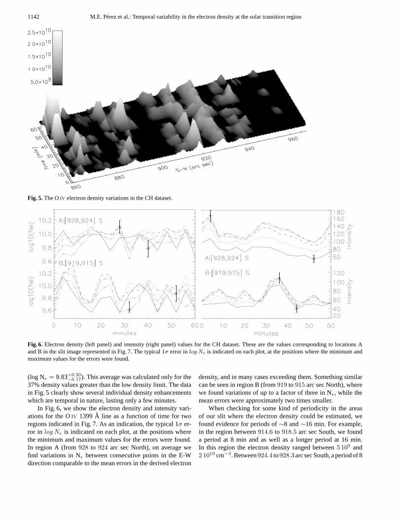
The Northern CH dataset, centered at (0, 910) arc sec, startedat 01:07:23UT and ended at 02:14:04UT on 14 July 1996 andhad an exposure time of 20s. Since our image is in fact a tempo-ral series for the observational period (∼1h7min), the total areacovered by this dataset was∼1.5×112 arc sec2. The variationsof the electron density values for each position along the slitwith time is shown in Fig. 5. The allowed range of values forthe grey scale is between3.6 109 and2.5 1010 cm−3, with the av-erage electron density for the whole image being6.8 109 cm−3

2 sohowww.nascom.nasa.gov/instruments.html

1142 M.E. Perez et al.: Temporal variability in the electron density at the solar transition region

Fig. 5. The Oiv electron density variations in the CH dataset.

Fig. 6. Electron density (left panel) and intensity (right panel) values for the CH dataset. These are the values corresponding to locations Aand B in the slit image represented in Fig. 7. The typical 1σ error in log Ne is indicated on each plot, at the positions where the minimum andmaximum values for the errors were found.

(log Ne = 9.83+0.20−0.17). This average was calculated only for the

37% density values greater than the low density limit. The datain Fig. 5 clearly show several individual density enhancementswhich are temporal in nature, lasting only a few minutes.

In Fig. 6, we show the electron density and intensity vari-ations for the Oiv 1399A line as a function of time for tworegions indicated in Fig. 7. As an indication, the typical 1σ er-ror in log Ne is indicated on each plot, at the positions wherethe minimum and maximum values for the errors were found.In region A (from928 to 924 arc sec North), on average wefind variations in Ne between consecutive points in the E-Wdirection comparable to the mean errors in the derived electron

density, and in many cases exceeding them. Something similarcan be seen in region B (from919 to 915 arc sec North), wherewe found variations of up to a factor of three in Ne, while themean errors were approximately two times smaller.

When checking for some kind of periodicity in the areasof our slit where the electron density could be estimated, wefound evidence for periods of∼8 and∼16 min. For example,in the region between914.6 to 918.5 arc sec South, we founda period at 8 min and as well as a longer period at 16 min.In this region the electron density ranged between5 109 and2 1010 cm−3. Between924.4 to928.3arc sec South, a period of 8

M.E. Perez et al.: Temporal variability in the electron density at the solar transition region 1143

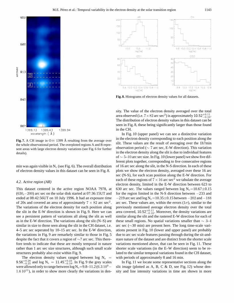
Fig. 7. A CH image in Oiv 1399A resulting from the average overthe whole observational period. The overploted regions A and B repre-sent areas with large electron density variations (see Fig. 6 for furtherdetails).

min was again visible in Ne (see Fig. 6). The overall distributionof electron density values in this dataset can be seen in Fig. 8.

4.2. Active region (AR)

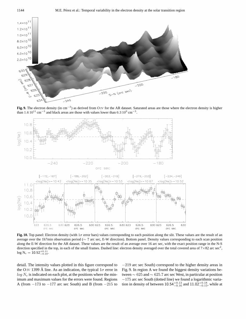
This dataset centered in the active region NOAA 7978, at(630,−200) arc sec on the solar disk started at 07:36:15UT andended at 08:42:56UT on 10 July 1996. It had an exposure timeof 20s and covered an area of approximately7 × 82 arc sec2.The variations of the electron density for each position alongthe slit in the E-W direction is shown in Fig. 9. Here we cansee a persistent pattern of variations all along the slit as wellas in the E-W direction. The variations along the slit (N–S) aresimilar in size to those seen along the slit in the CH dataset, i.e.4–5 arc sec seperated by 10–15 arc sec. In the E-W direction,the variations in Fig. 9 are remarkely similar to those in Fig. 5despite the fact that it covers a region of∼7 arc sec. This there-fore tends to indicate that these are mostly temporal in naturerather than 1 arc sec size structures, although such small scalestructures probably also exist within Fig. 9.

The electron density values ranged between log Ne =9.56+0.28

−0.25 and log Ne = 11.45+0.23−0.18. In Fig. 9 the grey scales

were allowed only to range between log Ne=9.8–11.2 (6.3 109−1.6 1011), in order to show more clearly the variations in den-

Fig. 8. Histograms of electron density values for all datasets.

sity. The value of the electron density averaged over the totalarea observed (i.e.7×82 arc sec2) is approximately10.52+0.11

−0.10.The distribution of electron density values in this dataset can beseen in Fig. 8, these being significantly larger than those foundin the CH.

In Fig. 10 (upper panel) we can see a distinctive variationin the electron density corresponding to each position along theslit. These values are the result of averaging over the 1h7minobservation period (∼ 7 arc sec, E-W direction). This variationin the electron density along the slit is due to individual featuresof ∼ 5–10 arc sec size. In Fig. 10 (lower panel) we show five dif-ferent plots together, corresponding to five consecutive regionsof 16 arc sec along the slit, in the N-S direction. In each of theseplots we show the electron density, averaged over these 16 arcsec (N-S), for each scan position along the E-W direction. Foreach of these regions of7× 16 arc sec2 we tabulate the averageelectron density, limited in the E-W direction between 623 to630 arc sec. The values ranged between log Ne=10.67±0.15for the region limited in the N-S direction between−233 and−219 arc sec and log Ne=10.35±0.15 between−202 and−188arc sec. These values are, within the errors (1σ), similar to thepreviously mentioned average electron density over the totalarea covered,10.52+0.11

−0.10. Moreover, the density variations aresimilar along the slit and the rastered E-W direction for each ofthese small regions. No spatial variations smaller than∼ 3–4arc sec (∼30 min) are present here. The long time-scale vari-ations present in Fig. 10 (lower and upper panel) are probablydue to arc sec scale features passing through during the sit-and-stare nature of the dataset and are distinct from the shorter scalevariations mentioned above, that can be seen in Fig. 11. Theseshorter scale variations (in the E–W direction) seem to be re-lated to the similar temporal variations found in the CH dataset,with periods of approximately 8 and 16 min.

In Fig. 11 we locate some representative sections along theslit image (plotted as A, B, C & D, seeFig. 12) whose den-sity and line intensity variations in time are shown in more

1144 M.E. Perez et al.: Temporal variability in the electron density at the solar transition region

Fig. 9. The electron density (in cm−3) as derived from Oiv for the AR dataset. Saturated areas are those where the electron density is higherthan1.6 1011 cm−3 and black areas are those with values lower than6.3 109 cm−3.

Fig. 10.Top panel: Electron density (with1σ error bars) values corresponding to each position along the slit. These values are the result of anaverage over the 1h7min observation period (∼ 7 arc sec, E-W direction). Bottom panel. Density values corresponding to each scan positionalong the E-W direction for the AR dataset. These values are the result of an average over 16 arc sec, with the exact position range in the N-Sdirection specified in the top, in each of the small frames. Dashed line: electron density averaged over the total covered area of 7×82 arc sec2,log Ne = 10.52+0.11

−0.10.

detail. The intensity values plotted in this figure correspond tothe Oiv 1399A line. As an indication, the typical 1σ error inlog Ne is indicated on each plot, at the positions where the min-imum and maximum values for the errors were found. RegionsA (from −173 to −177 arc sec South) and B (from−215 to

−219 arc sec South) correspond to the higher density areas inFig. 9. In region A we found the biggest density variations be-tween∼ 625 and∼ 625.7 arc sec West, in particular at position−175 arc sec South (dotted line) we found a logarithmic varia-tion in density of between10.54+0.13

−0.16 and11.02+0.18−0.15, while at

M.E. Perez et al.: Temporal variability in the electron density at the solar transition region 1145

Fig. 11.Some of the electron density and intensity values for the AR dataset. These are the values corresponding to locations A, B, C and Din the slit image represented in Fig. 12. The exact range in arc sec is given here in brackets for each of these locations. The typical 1σ error inlog Ne is indicated on each plot, at the positions where the minimum and maximum values for the errors were found.

position−176 arc sec South (dashed line) there was a variationof between10.46+0.13

−0.15 and10.89+0.12−0.12. Between∼ 626.7 and

∼ 627.5 arc sec West, the variations were between10.92+0.12−0.11

and11.44+0.30−0.22 at −173 arc sec South (continuous line). In re-

gion B, between∼ 623.6 and∼ 624.5 arc sec West, we founda logarithmic variation in density of between10.94+0.08

−0.08 and11.45+0.23

−0.18 at −216 (dotted line) and−217 (dashed line) arcsec South. For this same area, between∼ 626.8 and∼ 627.5arc sec West, this variation was between the logaritmic values10.34+0.07

−0.08 and10.76+0.06−0.06 at −215 arc sec South (continuous

line). On average we found a variation of a factor of 1.5 in Ne

between consecutive positions E-W, that is over 0.44 arc sec,while the mean errors in the electron density were a factor oftwo less.

In region C (from−227 to −230 arc sec South), on averagewe found a variation of a factor of 1.3 between consecutive po-sitions E-W. For instance, we found from−227 to−230 arc secSouth variations of a factor of two in Ne between∼ 628.6 and∼ 629.7 arc sec West, i.e. within 1 arc sec, thus suggesting thatthese are temporal in nature. In region D (from−242 to −246

arc sec South), we find three areas in the E-W direction withvariations in the electron density greater than a factor of two;namely between∼ 624.2 and∼ 624.8 arc sec West, between∼ 626.4 and∼ 627.1 arc sec West, and between∼ 628.5 and∼ 629.2 arc sec West. Again, these are temporal in nature dueto the small area covered in the E-W direction.

When checking for some kind of periodicity we found that,while for some regions along the slit there was no appreciableperiodicity, for others there was evidence for approximately 0.8,1.1 and 1.6 arc sec periodicities which corresponds to∼8,∼11and∼16 min period. Our binning on the E-W direction was4 min which corresponds to∼0.4 arc sec. The longer periodsappear mainly in the northern half of the image, that is the lessintense part of the AR, although the electron densities are higherin this region. These were in areas of five arc sec (the runningmean for this analysis) at around−195 and−177 arc sec South.From −221 to −230.5 arc sec South there was evidence forperiodicities of 0.8 arc sec (8 min) and 1.1 arc sec (11 min) inthe density, that extended to approximately−245 arc sec (seealso Fig. 11).

1146 M.E. Perez et al.: Temporal variability in the electron density at the solar transition region

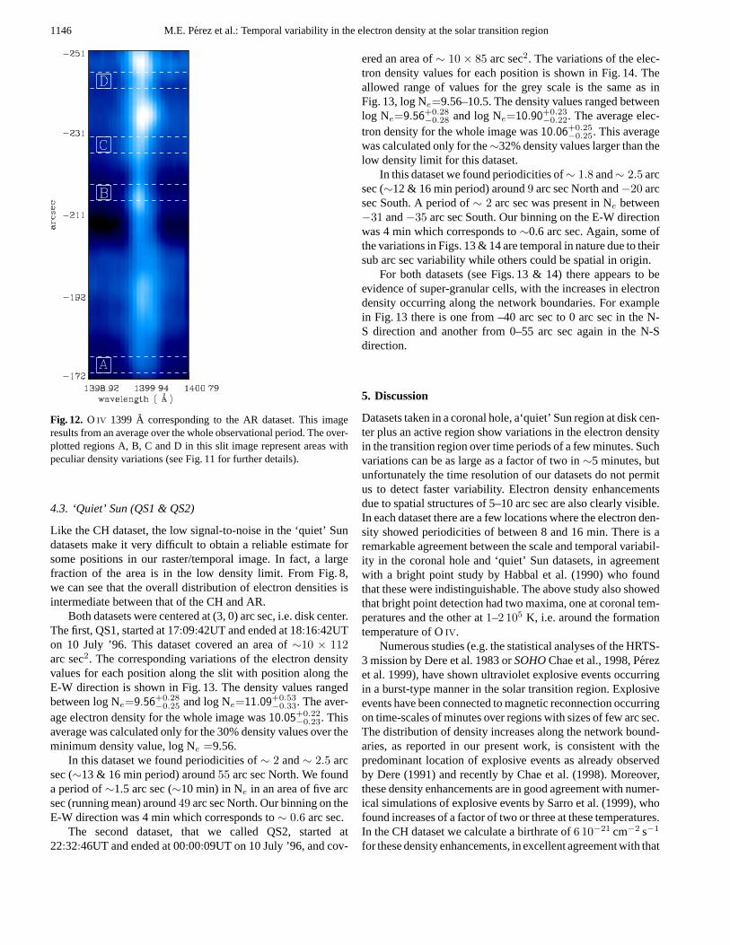
Fig. 12. O iv 1399 A corresponding to the AR dataset. This imageresults from an average over the whole observational period. The over-plotted regions A, B, C and D in this slit image represent areas withpeculiar density variations (see Fig. 11 for further details).

4.3. ‘Quiet’ Sun (QS1 & QS2)

Like the CH dataset, the low signal-to-noise in the ‘quiet’ Sundatasets make it very difficult to obtain a reliable estimate forsome positions in our raster/temporal image. In fact, a largefraction of the area is in the low density limit. From Fig. 8,we can see that the overall distribution of electron densities isintermediate between that of the CH and AR.

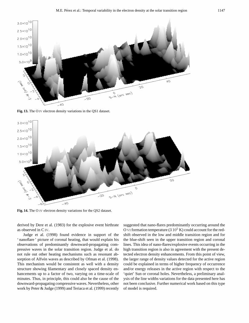
Both datasets were centered at (3, 0) arc sec, i.e. disk center.The first, QS1, started at 17:09:42UT and ended at 18:16:42UTon 10 July ’96. This dataset covered an area of∼10 × 112arc sec2. The corresponding variations of the electron densityvalues for each position along the slit with position along theE-W direction is shown in Fig. 13. The density values rangedbetween log Ne=9.56+0.28

−0.25 and log Ne=11.09+0.53−0.33. The aver-

age electron density for the whole image was10.05+0.22−0.23. This

average was calculated only for the 30% density values over theminimum density value, log Ne =9.56.

In this dataset we found periodicities of∼ 2 and∼ 2.5 arcsec (∼13 & 16 min period) around55 arc sec North. We founda period of∼1.5 arc sec (∼10 min) in Ne in an area of five arcsec (running mean) around49 arc sec North. Our binning on theE-W direction was 4 min which corresponds to∼ 0.6 arc sec.

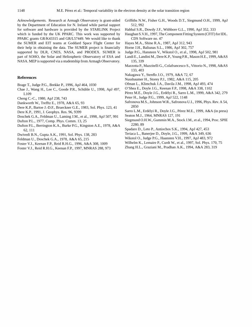
The second dataset, that we called QS2, started at22:32:46UT and ended at 00:00:09UT on 10 July ’96, and cov-

ered an area of∼ 10 × 85 arc sec2. The variations of the elec-tron density values for each position is shown in Fig. 14. Theallowed range of values for the grey scale is the same as inFig. 13, log Ne=9.56–10.5. The density values ranged betweenlog Ne=9.56+0.28

−0.28 and log Ne=10.90+0.23−0.22. The average elec-

tron density for the whole image was10.06+0.25−0.25. This average

was calculated only for the∼32% density values larger than thelow density limit for this dataset.

In this dataset we found periodicities of∼ 1.8 and∼ 2.5 arcsec (∼12 & 16 min period) around9 arc sec North and−20 arcsec South. A period of∼ 2 arc sec was present in Ne between−31 and−35 arc sec South. Our binning on the E-W directionwas 4 min which corresponds to∼0.6 arc sec. Again, some ofthe variations in Figs. 13 & 14 are temporal in nature due to theirsub arc sec variability while others could be spatial in origin.

For both datasets (see Figs. 13 & 14) there appears to beevidence of super-granular cells, with the increases in electrondensity occurring along the network boundaries. For examplein Fig. 13 there is one from –40 arc sec to 0 arc sec in the N-S direction and another from 0–55 arc sec again in the N-Sdirection.

5. Discussion

Datasets taken in a coronal hole, a‘quiet’ Sun region at disk cen-ter plus an active region show variations in the electron densityin the transition region over time periods of a few minutes. Suchvariations can be as large as a factor of two in∼5 minutes, butunfortunately the time resolution of our datasets do not permitus to detect faster variability. Electron density enhancementsdue to spatial structures of 5–10 arc sec are also clearly visible.In each dataset there are a few locations where the electron den-sity showed periodicities of between 8 and 16 min. There is aremarkable agreement between the scale and temporal variabil-ity in the coronal hole and ‘quiet’ Sun datasets, in agreementwith a bright point study by Habbal et al. (1990) who foundthat these were indistinguishable. The above study also showedthat bright point detection had two maxima, one at coronal tem-peratures and the other at1–2 105 K, i.e. around the formationtemperature of Oiv.

Numerous studies (e.g. the statistical analyses of the HRTS-3 mission by Dere et al. 1983 orSOHOChae et al., 1998, Perezet al. 1999), have shown ultraviolet explosive events occurringin a burst-type manner in the solar transition region. Explosiveevents have been connected to magnetic reconnection occurringon time-scales of minutes over regions with sizes of few arc sec.The distribution of density increases along the network bound-aries, as reported in our present work, is consistent with thepredominant location of explosive events as already observedby Dere (1991) and recently by Chae et al. (1998). Moreover,these density enhancements are in good agreement with numer-ical simulations of explosive events by Sarro et al. (1999), whofound increases of a factor of two or three at these temperatures.In the CH dataset we calculate a birthrate of6 10−21 cm−2 s−1

for these density enhancements, in excellent agreement with that

M.E. Perez et al.: Temporal variability in the electron density at the solar transition region 1147

Fig. 13.The Oiv electron density variations in the QS1 dataset.

Fig. 14.The Oiv electron density variations for the QS2 dataset.

derived by Dere et al. (1983) for the explosive event birthrateas observed in Civ.

Judge et al. (1998) found evidence in support of the‘ nanoflare ’ picture of coronal heating, that would explain hisobservations of predominantly downward-propagating com-pressive waves in the solar transition region. Judge et al. donot rule out other heating mechanisms such as resonant ab-sorption of Alfven waves as described by Ofman et al. (1998).This mechanism would be consistent as well with a densitystructure showing filamentary and closely spaced density en-hancements up to a factor of two, varying on a time-scale ofminutes. Thus, in principle, this could also be the cause of thedownward-propagating compressive waves. Nevertheless, otherwork by Peter & Judge (1999) and Teriaca et al. (1999) recently

suggested that nano-flares predominantly occurring around theOvi formation temperature (3 105 K) could account for the red-shift observed in the low and middle transition region and forthe blue-shift seen in the upper transition region and coronallines. This idea of nano-flares/explosive events occurring in thehigh transition region is also in agreement with the present de-tected electron density enhancements. From this point of view,the larger range of density values detected for the active regioncould be explained in terms of higher frequency of occurrenceand/or energy releases in the active region with respect to the‘quiet’ Sun or coronal holes. Nevertheless, a preliminary anal-ysis of the line widths variations for the data presented here hasnot been conclusive. Further numerical work based on this typeof model is required.

1148 M.E. Perez et al.: Temporal variability in the electron density at the solar transition region

Acknowledgements.Research at Armagh Observatory is grant-aidedby the Department of Education for N. Ireland while partial supportfor software and hardware is provided by the STARLINK Projectwhich is funded by the UK PPARC. This work was supported byPPARC grants GR/K43315 and GR/L57449. We would like to thankthe SUMER and EIT teams at Goddard Space Flight Center fortheir help in obtaining the data. The SUMER project is financiallysupported by DLR, CNES, NASA, and PRODEX. SUMER ispart of SOHO, the Solar and Heliospheric Observatory of ESA andNASA. MEP is supported via a studentship from Armagh Observatory.

References

Brage T., Judge P.G., Brekke P., 1996, ApJ 464, 1030Chae J., Wang H., Lee C., Goode P.R., Schuhle U., 1998, ApJ 497,

L109Cheng C.-C., 1980, ApJ 238, 743Dankworth W., Trefftz E., 1978, A&A 65, 93Dere K.P., Bartoe J.-D.F., Brueckner G.E., 1983, Sol. Phys. 123, 41Dere K.P., 1991, J. Geophys. Res. 96, 9399Doschek G.A., Feldman U., Laming J.M., et al., 1998, ApJ 507, 991Dufton P.L., 1977, Comp. Phys. Comm. 13, 25Dufton P.L., Berrington K.A., Burke P.G., Kingston A.E., 1978, A&A

62, 111Dwivedi B.N., Gupta A.K., 1991, Sol. Phys. 138, 283Feldman U., Doschek G.A., 1978, A&A 65, 215Foster V.J., Keenan F.P., Reid R.H.G., 1996, A&A 308, 1009Foster V.J., Reid R.H.G., Keenan F.P., 1997, MNRAS 288, 973

Griffiths N.W., Fisher G.H., Woods D.T., Siegmund O.H., 1999, ApJ512, 992

Habbal S.R., Dowdy J.F., Withbore G.L., 1990, ApJ 352, 333Haughan S.V.H., 1997, The Component Fitting System (CFIT) for IDL.

CDS Software no. 47Hayes M.A., Shine R.A., 1987, ApJ 312, 943Horne J.H., Baliunas S.L., 1986, ApJ 302, 757Judge P.G., Hansteen V., Wikstol O., et al., 1998, ApJ 502, 981Landi E., Landini M., Dere K.P., Young P.R., Mason H.E., 1999, A&AS

135, 339Mazzotta P., Mazzitelli G., Colafrancesco S., Vittorio N., 1998, A&AS

133, 403Nakagawa Y., Stenflo J.O., 1979, A&A 72, 67Nussbaumer H., Storey P.J., 1982, A&A 115, 205Ofman L., Klimchuk J.A., Davila J.M., 1998, ApJ 493, 474O’Shea E., Doyle J.G., Keenan F.P., 1998, A&A 338, 1102Perez M.E., Doyle J.G., Erdelyi R., Sarro L.M., 1999, A&A 342, 279Peter H., Judge P.G., 1999, ApJ 522, 1148Safronova M.S., Johnson W.R., Safronova U.I., 1996, Phys. Rev. A 54,

2850Sarro L.M., Erdelyi R., Doyle J.G., Perez M.E., 1999, A&A (in press)Seaton M.J., 1964, MNRAS 127, 191Siegmund O.H.W., Gummin M.A., Stock J.M., et al., 1994, Proc. SPIE

2280, 89Spadaro D., Leto P., Antiochos S.K., 1994, ApJ 427, 453Teriaca L., Banerjee D., Doyle, J.G., 1999, A&A 349, 636Wikstol O., Judge P.G., Haansten V.H., 1997, ApJ 483, 972Wilhelm K., Lemaire P., Curdt W., et al., 1997, Sol. Phys. 170, 75Zhang H.L., Graziani M., Pradhan A.K., 1994, A&A 283, 319