AST242 LECTURE NOTES PART 1 Contentsastro.pas.rochester.edu/~aquillen/ast242/lecturenotes1.pdf · 4 AST242 LECTURE NOTES PART 1 Figure 2. Streamlines, paths and streaks. Another example

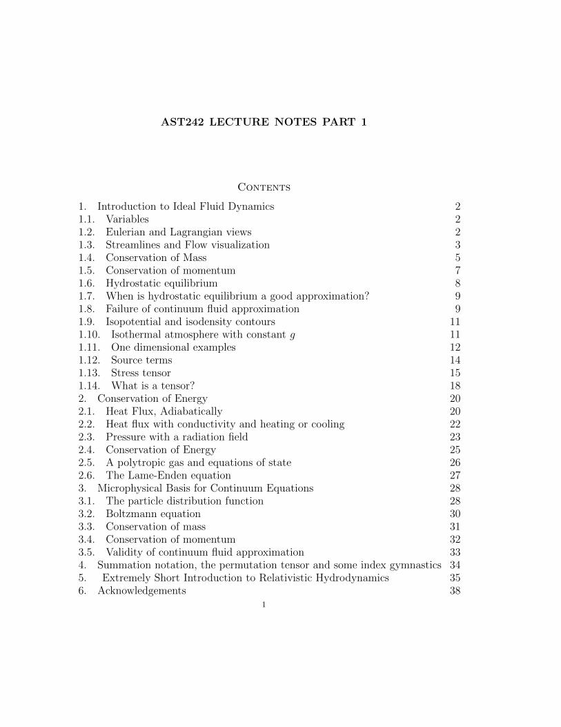
AST242 LECTURE NOTES PART 1

Contents

1. Introduction to Ideal Fluid Dynamics 21.1. Variables 21.2. Eulerian and Lagrangian views 21.3. Streamlines and Flow visualization 31.4. Conservation of Mass 51.5. Conservation of momentum 71.6. Hydrostatic equilibrium 81.7. When is hydrostatic equilibrium a good approximation? 91.8. Failure of continuum fluid approximation 91.9. Isopotential and isodensity contours 111.10. Isothermal atmosphere with constant g 111.11. One dimensional examples 121.12. Source terms 141.13. Stress tensor 151.14. What is a tensor? 182. Conservation of Energy 202.1. Heat Flux, Adiabatically 202.2. Heat flux with conductivity and heating or cooling 222.3. Pressure with a radiation field 232.4. Conservation of Energy 252.5. A polytropic gas and equations of state 262.6. The Lame-Enden equation 273. Microphysical Basis for Continuum Equations 283.1. The particle distribution function 283.2. Boltzmann equation 303.3. Conservation of mass 313.4. Conservation of momentum 323.5. Validity of continuum fluid approximation 334. Summation notation, the permutation tensor and some index gymnastics 345. Extremely Short Introduction to Relativistic Hydrodynamics 356. Acknowledgements 38

1

2 AST242 LECTURE NOTES PART 1

1. Introduction to Ideal Fluid Dynamics

1.1. Variables. A fluid is characterized by a mean velocity field u(x, t) and at leasttwo integrated or thermodynamic quantities. Often these are the mass density, ρ(x, t)and pressure p(x, t). The energy density e, or temperature, T , can treated as anadditional variable or can be related to ρ and p.

There can be additional degrees of freedom, such as the molecular or nuclearcomposition and the ionization state.

1.2. Eulerian and Lagrangian views. We view the system from a fixed coordinatesystem and describe each variable as a function of (x, t). The partial time derivative

∂

∂t

describes how variables change in time from the point of view of a fixed point inspace attached to a coordinate system or an inertial frame. This is the Eulerianviewpoint.

We could also describe the system from the view point of particles moving withthe fluid. Suppose we have a scalar quantity like T . We would like to predict whatwould cause a small change δT as our fluid element moves. Over a small change intime δt and with small changes in coordinates δx, δy, δz.

δT =∂T

∂tδt+

∂T

∂xδx+

∂T

∂yδy +

∂T

∂zδz

We now divide by δt.

(1)δT

δt=∂T

∂t+∂T

∂x

δx

δt+∂T

∂y

δy

δt+∂T

∂z

δz

δt

If we chose δx, δy, δt to be an element of the fluid that is moving along with the fluidthen δx

δt= u and we can write the above as

δT

δt=∂T

∂t+ u ·∇T

If we consider derivatives from the point of view of particles moving with the fluidthen we can describe changes with the Lagrangian time-derivative or

D

Dt=

∂

∂t+ u ·∇

Let us write this out in terms of components

D

Dt=

∂

∂t+∑i

ui∂

∂xi

as we had done in equation (56).

AST242 LECTURE NOTES PART 1 3

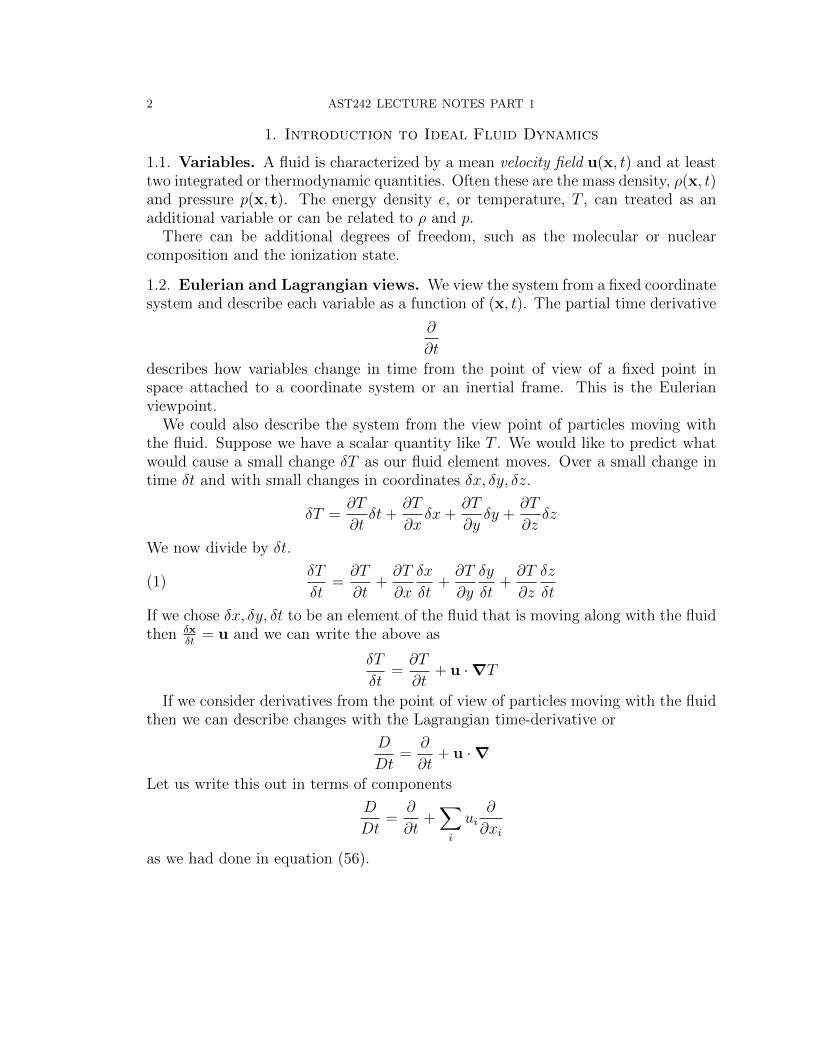
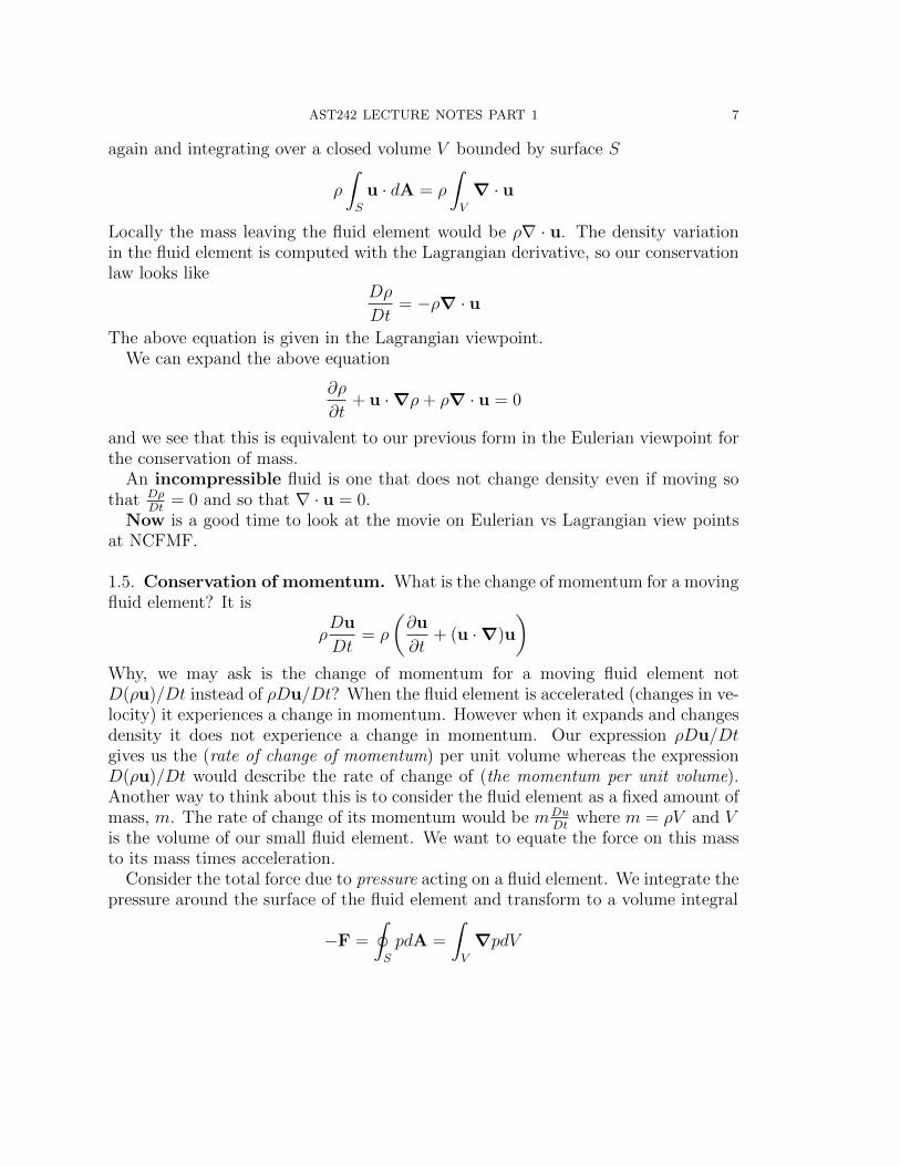
Figure 1. A fluid element moving within a larger flow.

Another way to think about this is to consider a fluid element at x that has movedby uδt in a time δt. If we consider T for that fluid element we can write T as

T (x + uδt, t+ δt)

so the change in T moving with the fluid element

DT

Dt= lim

δt→0

(T (x + uδt, t+ δt)− T (x, t)

δt

)=

[∂

∂t+ u ·∇

]T

If we write equations from the view point of fluid elements that are moving we saywe are using the Lagrangian view point.

Consider traffic flow. We can describe traffic flow in terms of density, ρ, (cars perunit length) and a velocity, u, the speed of cars on the road. If we describe ρ andu as a function of position on the road we are using the Eulerian view point. If wedescribe ρ and u in terms of those seen by individual drivers we say we are using theLagrangian viewpoint.

Numerical methods that use fixed grids work in the Eulerian view point. Numericalmethods that allow particles to move in the simulation and compute forces on theseparticles work in the Lagrangian viewpoint. Smooth Particle Hydrodynamics (SPH)codes use the Lagrangian viewpoint.

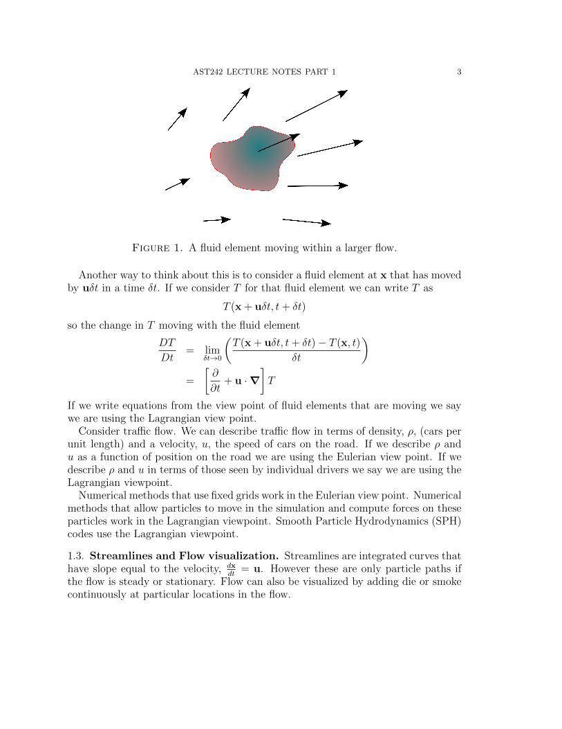
1.3. Streamlines and Flow visualization. Streamlines are integrated curves thathave slope equal to the velocity, dx

dt= u. However these are only particle paths if

the flow is steady or stationary. Flow can also be visualized by adding die or smokecontinuously at particular locations in the flow.


Figure 2. Streamlines, paths and streaks.

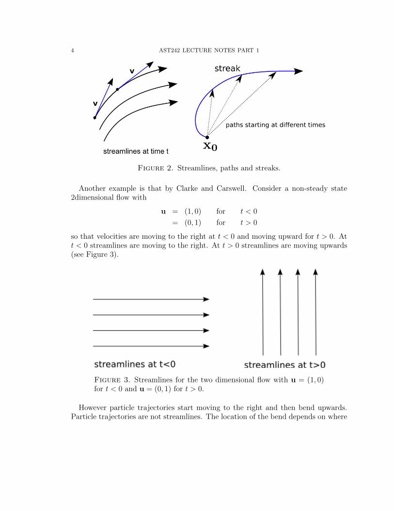
Another example is that by Clarke and Carswell. Consider a non-steady state2dimensional flow with

u = (1, 0) for t < 0

= (0, 1) for t > 0

so that velocities are moving to the right at t < 0 and moving upward for t > 0. Att < 0 streamlines are moving to the right. At t > 0 streamlines are moving upwards(see Figure 3).

Figure 3. Streamlines for the two dimensional flow with u = (1, 0)for t < 0 and u = (0, 1) for t > 0.

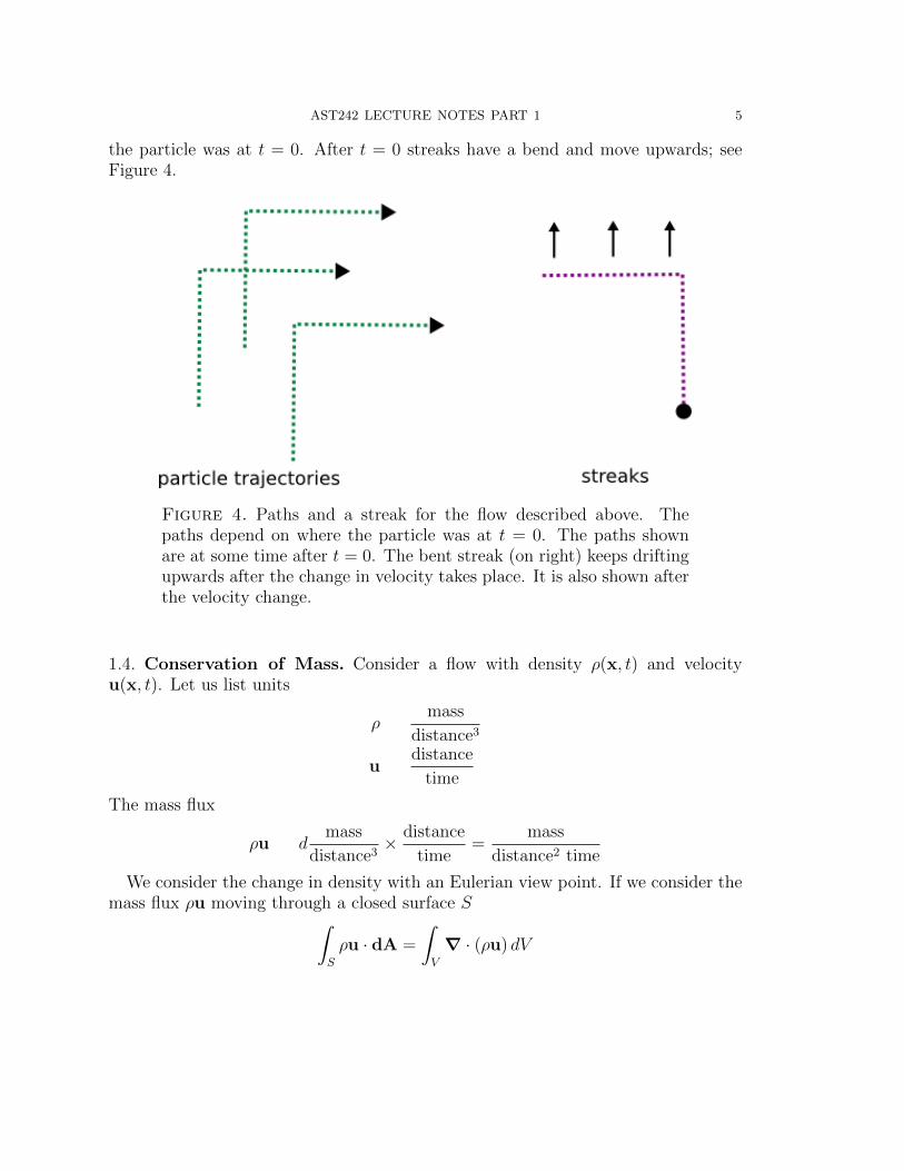
However particle trajectories start moving to the right and then bend upwards.Particle trajectories are not streamlines. The location of the bend depends on where


the particle was at t = 0. After t = 0 streaks have a bend and move upwards; seeFigure 4.

Figure 4. Paths and a streak for the flow described above. Thepaths depend on where the particle was at t = 0. The paths shownare at some time after t = 0. The bent streak (on right) keeps driftingupwards after the change in velocity takes place. It is also shown afterthe velocity change.

1.4. Conservation of Mass. Consider a flow with density ρ(x, t) and velocityu(x, t). Let us list units

ρmass

distance3

udistance

time

The mass flux

ρu dmass

distance3× distance

time=

mass

distance2 time

We consider the change in density with an Eulerian view point. If we consider themass flux ρu moving through a closed surface S∫

S

ρu · dA =

∫V

∇ · (ρu) dV


Figure 5. For a flow with density ρ and velocity u the mass flowthrough a surface oriented in direction dA and with area |dA| is ρu·dA.

where I have used Gaus’s law to write this as an integral over a volume V enclosedby the surface S. The mass flux through the surface S must be balanced by changeof density in V or ∫

V

∂ρ

∂tdV = −

∫V

∇ · (ρu) dV

Equating the two expressions (locally)

∂ρ

∂t+ ∇ · (ρu) = 0

This is the general form for a conservation law for a scalar quantity, which in thiscase is the mass density ρ.

We can write a conservation law in the form

∂

∂t(quantity) + ∇ · (flux of quantity) = 0.

Our example for conservation of mass is a scalar. However when we discuss momen-tum we can consider more general (vector or tensor) forms for conservation laws.

Some numerical algorithms require putting differential equations in conservationlaw form. The above equation does not involve a Lagrangian derivative and so is inthe Eulerian view point.

Consider the form of the conservation of mass using the Lagrangian viewpoint.The mass flux of a fluid element moving with the fluid is reduced if there is massleaving the fluid element boundary. The rate that mass leaves the fluid elementdepends on the velocity field and the density in the fluid element. Using Gaus’s law


again and integrating over a closed volume V bounded by surface S

ρ

∫S

u · dA = ρ

∫V

∇ · u

Locally the mass leaving the fluid element would be ρ∇ · u. The density variationin the fluid element is computed with the Lagrangian derivative, so our conservationlaw looks like

Dρ

Dt= −ρ∇ · u

The above equation is given in the Lagrangian viewpoint.We can expand the above equation

∂ρ

∂t+ u ·∇ρ+ ρ∇ · u = 0

and we see that this is equivalent to our previous form in the Eulerian viewpoint forthe conservation of mass.

An incompressible fluid is one that does not change density even if moving sothat Dρ

Dt= 0 and so that ∇ · u = 0.

Now is a good time to look at the movie on Eulerian vs Lagrangian view pointsat NCFMF.

1.5. Conservation of momentum. What is the change of momentum for a movingfluid element? It is

ρDu

Dt= ρ

(∂u

∂t+ (u ·∇)u

)Why, we may ask is the change of momentum for a moving fluid element notD(ρu)/Dt instead of ρDu/Dt? When the fluid element is accelerated (changes in ve-locity) it experiences a change in momentum. However when it expands and changesdensity it does not experience a change in momentum. Our expression ρDu/Dtgives us the (rate of change of momentum) per unit volume whereas the expressionD(ρu)/Dt would describe the rate of change of (the momentum per unit volume).Another way to think about this is to consider the fluid element as a fixed amount ofmass, m. The rate of change of its momentum would be mDu

Dtwhere m = ρV and V

is the volume of our small fluid element. We want to equate the force on this massto its mass times acceleration.

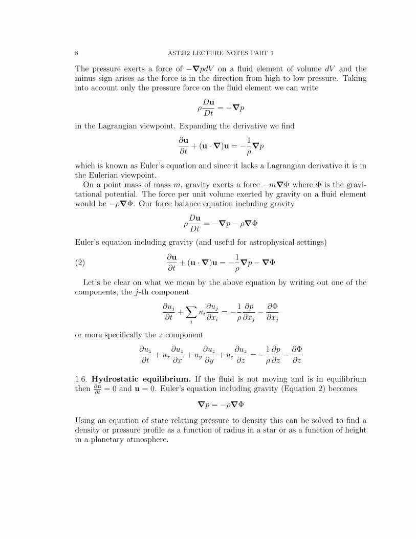
Consider the total force due to pressure acting on a fluid element. We integrate thepressure around the surface of the fluid element and transform to a volume integral

−F =

∮S

pdA =

∫V

∇pdV


The pressure exerts a force of −∇pdV on a fluid element of volume dV and theminus sign arises as the force is in the direction from high to low pressure. Takinginto account only the pressure force on the fluid element we can write

ρDu

Dt= −∇p

in the Lagrangian viewpoint. Expanding the derivative we find

∂u

∂t+ (u ·∇)u = −1

ρ∇p

which is known as Euler’s equation and since it lacks a Lagrangian derivative it is inthe Eulerian viewpoint.

On a point mass of mass m, gravity exerts a force −m∇Φ where Φ is the gravi-tational potential. The force per unit volume exerted by gravity on a fluid elementwould be −ρ∇Φ. Our force balance equation including gravity

ρDu

Dt= −∇p− ρ∇Φ

Euler’s equation including gravity (and useful for astrophysical settings)

(2)∂u

∂t+ (u ·∇)u = −1

ρ∇p−∇Φ

Let’s be clear on what we mean by the above equation by writing out one of thecomponents, the j-th component

∂uj∂t

+∑i

ui∂uj∂xi

= −1

ρ

∂p

∂xj− ∂Φ

∂xj

or more specifically the z component

∂uz∂t

+ ux∂uz∂x

+ uy∂uz∂y

+ uz∂uz∂z

= −1

ρ

∂p

∂z− ∂Φ

∂z

1.6. Hydrostatic equilibrium. If the fluid is not moving and is in equilibriumthen ∂u

∂t= 0 and u = 0. Euler’s equation including gravity (Equation 2) becomes

∇p = −ρ∇Φ

Using an equation of state relating pressure to density this can be solved to find adensity or pressure profile as a function of radius in a star or as a function of heightin a planetary atmosphere.


1.7. When is hydrostatic equilibrium a good approximation? A planetaryatmosphere may be turbulent and so not perfectly static. We can ask when is itjustified to drop the first two terms in Euler’s equation? Let’s do some dimensionalanalysis on Euler’s equation. Recall Euler’s equation including gravity,

∂u

∂t+ u ·∇u = −1

ρ∇p−∇Φ

The term∂u

∂t∼ δu

δt∼ (δu)2

lwhere δu is the velocity of a typical turbulent motion of eddy size l that would lasta time δt ∼ l/δu. The term

u · ∇u ∼ (δu)2

lis of the same order of magnitude. The pressure term

1

ρ∇p ∼ c2s

h

where h is the atmosphere scale height and cs the sound speed. The gravity term

|∇Φ| = g

the acceleration due to gravity. We expect we can neglect the velocity terms inEuler’s equation when they are small compared to the pressure and gravity terms.We find that hydrostatic equilibrium is a good approximation as long as

(δu)2

l g

This is equivalent to saying accelerations in the eddies are smaller than that due togravity. The other condition would be

(δu)2

l c2s

hwhich for large eddies is equivalent to saying that eddies are subsonic.

1.8. Failure of continuum fluid approximation. Above we considered when ve-locity perturbations make hydrostatic equilibrium a bad approximation. Hydrostaticequilibrium is based on a continuum fluid approximation. The continuum fluid ap-proximation is no longer valid on a lengthscale shorter than the mean free path ofa particle or on a timescale shorter than the mean collision timescale. Consider thegas number density (particles per unit volume),

n =ρ

µmp


where µ is the mean molecular weight and mp the mass of a proton (we should beusing an atomic mass unit but that is approximately the mass of a proton). If thegas is molecular then we should correct the above to take into account the mass ofthe average molecule. Given a collision cross section σ and a gas number density n,the mean collision timescale

τcol = (nvσ)−1

where v is a mean velocity usually set by the temperature, and of order v ∼ cs. Themean free path is

(3) λ ∼ vτcol ∼ (nσ)−1

Since our fluid approximation fails on length scales shorter than the mean free path,our hydrostatic equilibrium approximation would fail when the atmospheric scaleheight h < λ.

To evaluate collision timescales or the mean free path an estimate for the crosssection is required. For molecules typically

σmolecules ∼ 10−15cm2

(Note the Bohr radius is 5× 10−9 cm.)In astrophysics we often have an ionized gas, but Coulomb interactions have an

infinite range. However we can define an effective radius, reff , for an encounter with

e2

reff∼ kBT

were e is the electron charge. Our cross section σ ∼ r2eff . The previous equation andequation 3 gives us a mean free path

λ ∼ n−1e e−4(kBT )2

where ne is the electron density and a timescale using the thermal velocity vthermal ∼√kBT/me of

τcol ∼ λ/vthermal ∼m

1/2e (kBT )3/2

nee4∼ 0.9 T 3/2n−1e second

Note the interesting temperature dependence. We will see similar temperature de-pendence in astrophysical settings where collisions are important such as radiativecooling, ionization and recombination, and conduction.


1.9. Isopotential and isodensity contours. Consider our equation for hydro-static equilibrium

∇p = −ρ∇Φ

Take the curl of both sides of the equation

0 = ∇× (ρ∇Φ) = ∇ρ×∇Φ + ρ∇×∇Φ

or

∇ρ×∇Φ = 0

Taken the length of both sides of the equation

|∇ρ||∇Φ| sin θ = 0

where sin θ is the angle between the two gradients. The angle θ must be 0 or π.This implies that isopotential contours are the same as isodensity contours (evenunderwater). Furthermore the equation ∇p = ρ∇Φ implies that isopressure contours(isobars) are the same as isopotential contours. We could describe any of p, ρ, or Φin terms of one of them, for example dP/dΦ = −ρ(Φ).

1.10. Isothermal atmosphere with constant g. For a small change in radius thegravitational potential is constant and the pressure at height z is the weight of thefluid above it

P (z) = g

∫ ∞z

ρ(z)dz

Assuming we have an idea gas, pressure is related to density and temperature withthe ideal gas law

p =ρkBT

µmp

Here kB is Boltzmann’s constant, mp the mass of the proton, p pressure, T tempera-ture, and µ the mean atomic weight. (Here mp loosely used as an atomic mass unit).If the atmosphere is isothermal then pressure is proportional to density;

p = Aρ

with constant A. Insert this into our equation for hydrostatic equilibrium (Euler’sequation neglecting velocity)


1

ρ∇p = −∇Φ

A

ρ

∂ρ

∂z= −g

∂

∂zln ρ = − g

A

ln ρ = −gzA

+ constant

and solution

ρ(z) = ρ0e− g(z−z0)

A

We call h = A/g the exponential scale height of the atmosphere. Checking units: Ais in units of velocity2 and g in units of velocity2/distance so the ratio gives a length.The constant A is approximately the sound speed in the gas. The scale heights ofthe atmospheres for the planets and planetesimals in our solar system can be quicklyestimated from their temperatures and surface gravities.

1.11. One dimensional examples. Recall Euler’s equation without gravity

∂u

∂t+ (u ·∇)u = −1

ρ∇p

Let’s write one component out completely, the z component.

∂uz∂t

+ ux∂uz∂x

+ uy∂uz∂y

+ uz∂uz∂z

= −1

ρ

∂p

∂z

Consider a one dimensional problem where quantities only vary in the z direction.The above equation reduces to

(4)∂uz∂t

+ uz∂uz∂z

= −1

ρ

∂p

∂z

The left hand side is the change of the velocity of a fluid element. The fluid elementslows down or speeds depending upon the pressure gradient it encounters. If the fluidelement encounters an increase in pressure then it slows down and if it encounters adecrease in pressure then it speeds up.

Consider what the equation looks like if the pressure gradient is zero. In this case

∂uz∂t

+ uz∂uz∂z

= 0

which we can write short hand

u,t + uu,z = 0


The above equation is a non-linear partial differential equation known as the inviscidBurger’s equation. Even in the most simplest case (zero pressure gradient and inone-dimension) we find a non-trivial non-linear equation.

Let’s go back to equation 4 but now assume that the system is steady state ortime independent so ∂u

∂t= 0. In this case

uu,z = −1

ρp,z

which we can write∂

∂z

(u2

2

)= −1

ρ

∂p

∂z

This illustrates that changes in pressure lead to corresponding changes in velocity.We will discuss this again in the context of Bernoulli’s equation.

Let’s consider our equation for conservation of mass.

∂ρ

∂t+ ∇ · u = 0

Now consider the above equation in one dimension

(5)∂ρ

∂t+

∂

∂z(ρuz) =

∂ρ

∂t+∂ρ

∂zuz +

∂uz∂z

ρ = 0

If we consider a fluid element with density ρ, this implies that only when there is avelocity gradient does the density of a fluid element increase or decrease. If we takethe above equation and consider the solution in steady state and divide by ρu theequation takes a useful form

(6)ρ,zρ

+u,zu

= 0

or

(7)d

dzln ρ+

d

dzlnu = 0

We can also write

(8)∂

∂z(ρu) = 0

so that a mass flux

(9) M = ρu

is independent of z. The above two examples show common manipulations of ourfluid equations in one dimension.

Often in astrophysics we will be working in spherical or cylindrical coordinatesand assuming that quantities only depend on radius. In this case our equation for


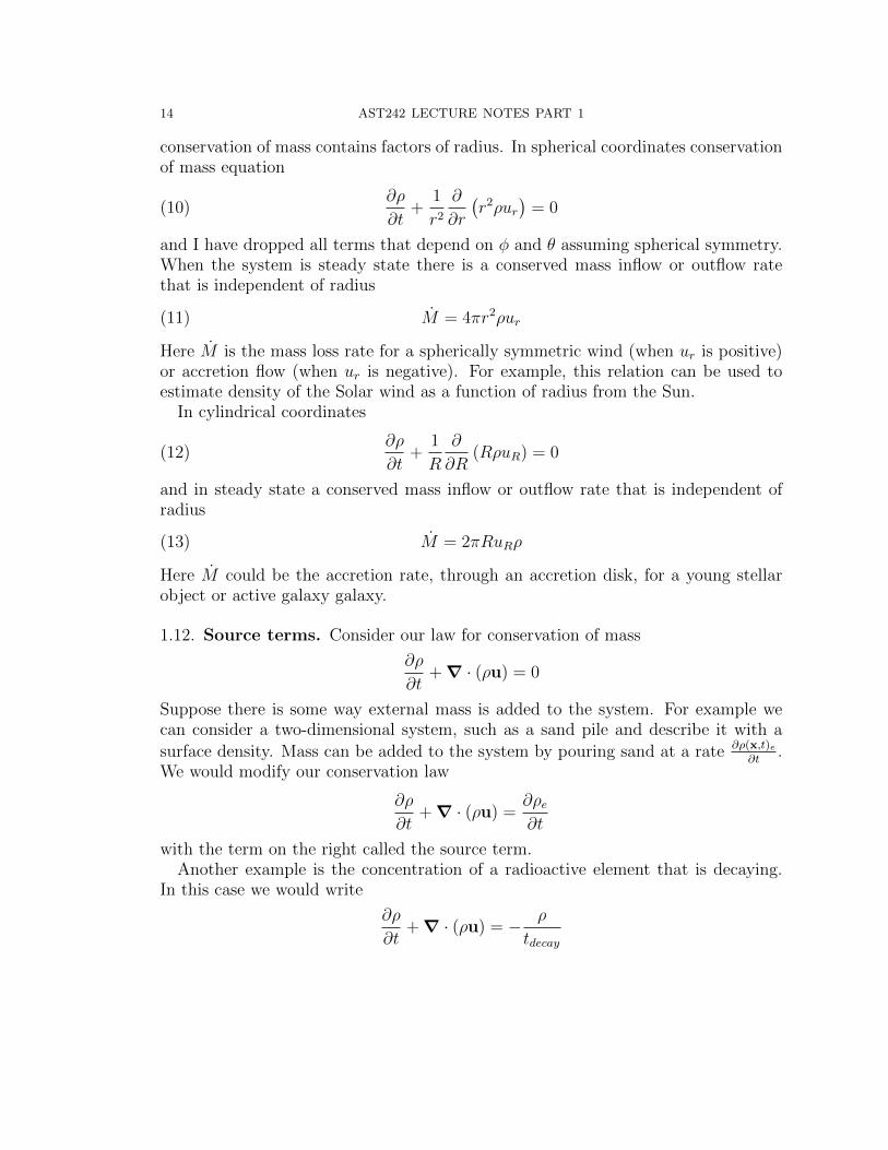
conservation of mass contains factors of radius. In spherical coordinates conservationof mass equation

(10)∂ρ

∂t+

1

r2∂

∂r

(r2ρur

)= 0

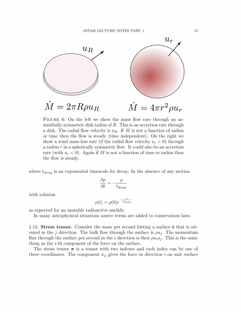
and I have dropped all terms that depend on φ and θ assuming spherical symmetry.When the system is steady state there is a conserved mass inflow or outflow ratethat is independent of radius

(11) M = 4πr2ρur

Here M is the mass loss rate for a spherically symmetric wind (when ur is positive)or accretion flow (when ur is negative). For example, this relation can be used toestimate density of the Solar wind as a function of radius from the Sun.

In cylindrical coordinates

(12)∂ρ

∂t+

1

R

∂

∂R(RρuR) = 0

and in steady state a conserved mass inflow or outflow rate that is independent ofradius

(13) M = 2πRuRρ

Here M could be the accretion rate, through an accretion disk, for a young stellarobject or active galaxy galaxy.

1.12. Source terms. Consider our law for conservation of mass

∂ρ

∂t+ ∇ · (ρu) = 0

Suppose there is some way external mass is added to the system. For example wecan consider a two-dimensional system, such as a sand pile and describe it with a

surface density. Mass can be added to the system by pouring sand at a rate ∂ρ(x,t)e∂t

.We would modify our conservation law

∂ρ

∂t+ ∇ · (ρu) =

∂ρe∂t

with the term on the right called the source term.Another example is the concentration of a radioactive element that is decaying.

In this case we would write

∂ρ

∂t+ ∇ · (ρu) = − ρ

tdecay


Figure 6. On the left we show the mass flow rate through an az-imuthally symmetric disk radius of R. This is an accretion rate througha disk. The radial flow velocity is uR. If M is not a function of radiusor time then the flow is steady (time independent). On the right weshow a wind mass loss rate (if the radial flow velocity ur > 0) througha radius r in a spherically symmetric flow. It could also be an accretionrate (with ur < 0). Again if M is not a function of time or radius thenthe flow is steady.

where tdecay is an exponential timescale for decay. In the absence of any motion

∂ρ

∂t= − ρ

tdecay

with solution

ρ(t) = ρ(0)e− ttdecay

as expected for an unstable radioactive nuclide.In many astrophysical situations source terms are added to conservation laws.

1.13. Stress tensor. Consider the mass per second hitting a surface s that is ori-ented in the j direction. The bulk flow through the surface is ρuj. The momentumflux through the surface per second in the i direction is then ρuiuj. This is the samething as the i-th component of the force on the surface.

The stress tensor π is a tensor with two indexes and each index can be one ofthree coordinates. The component πij gives the force in direction i on unit surface


with normal in direction j. The force in direction given by n

F = π · n or Fi =∑j

πijnj

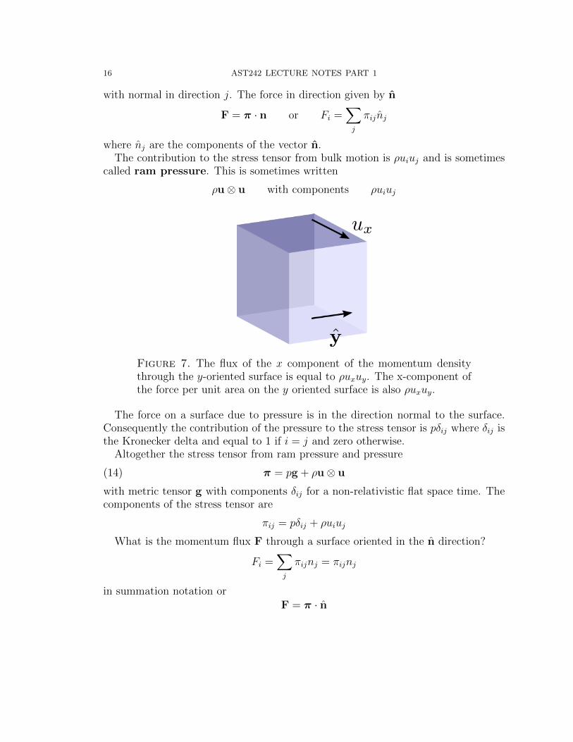
where nj are the components of the vector n.The contribution to the stress tensor from bulk motion is ρuiuj and is sometimes

called ram pressure. This is sometimes written

ρu⊗ u with components ρuiuj

Figure 7. The flux of the x component of the momentum densitythrough the y-oriented surface is equal to ρuxuy. The x-component ofthe force per unit area on the y oriented surface is also ρuxuy.

The force on a surface due to pressure is in the direction normal to the surface.Consequently the contribution of the pressure to the stress tensor is pδij where δij isthe Kronecker delta and equal to 1 if i = j and zero otherwise.

Altogether the stress tensor from ram pressure and pressure

(14) π = pg + ρu⊗ u

with metric tensor g with components δij for a non-relativistic flat space time. Thecomponents of the stress tensor are

πij = pδij + ρuiuj

What is the momentum flux F through a surface oriented in the n direction?

Fi =∑j

πijnj = πijnj

in summation notation orF = π · n


And all components individually

Fx = πxxnx + πxyny + πxznz

Fy = πyxnx + πyyny + πyznz

Fz = πzxnx + πzyny + πzznz

What is the force per unit area F on a surface with normal n? Identical to theabove expression.

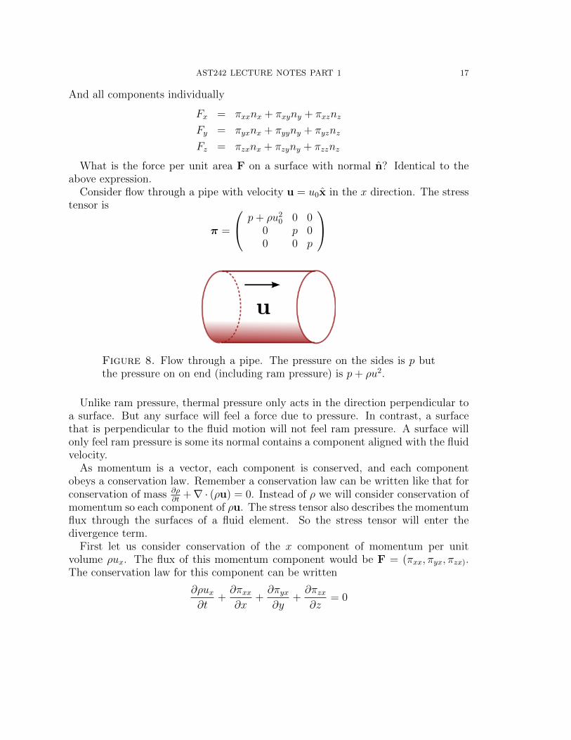
Consider flow through a pipe with velocity u = u0x in the x direction. The stresstensor is

π =

p+ ρu20 0 00 p 00 0 p

Figure 8. Flow through a pipe. The pressure on the sides is p butthe pressure on on end (including ram pressure) is p+ ρu2.

Unlike ram pressure, thermal pressure only acts in the direction perpendicular toa surface. But any surface will feel a force due to pressure. In contrast, a surfacethat is perpendicular to the fluid motion will not feel ram pressure. A surface willonly feel ram pressure is some its normal contains a component aligned with the fluidvelocity.

As momentum is a vector, each component is conserved, and each componentobeys a conservation law. Remember a conservation law can be written like that forconservation of mass ∂ρ

∂t+∇ · (ρu) = 0. Instead of ρ we will consider conservation of

momentum so each component of ρu. The stress tensor also describes the momentumflux through the surfaces of a fluid element. So the stress tensor will enter thedivergence term.

First let us consider conservation of the x component of momentum per unitvolume ρux. The flux of this momentum component would be F = (πxx, πyx, πzx).The conservation law for this component can be written

∂ρux∂t

+∂πxx∂x

+∂πyx∂y

+∂πzx∂z

= 0


We can describe conservation of all three momentum components all together with

∂(ρu)

∂t+ ∇ · π = 0

where ∇ ·π has j-th component =∑

i∂∂xiπij. The above equation is in conservation

law form but the conserved quantity is a vector ρu and the flux of the vector is atensor π.

In your problem set you will show that the above equation is consistent withEuler’s equation.

In the above equation we have neglected gravity. However the force due to gravitycan be included as a source term

(15)∂(ρu)

∂t+ ∇ · π = −ρ∇Φ

To make it clear what the notation means we will write out the j-th componentof this equation

∂(ρuj)

∂t+∑i

∂πij∂xi

= −ρ ∂Φ

∂xj

We use equation 14 for π to evaluate the second term term on the left using sum-mation notation (so dropping the

∑i)

∂πij∂xi

=∂(pδij)

∂xi+∂(ρuiuj)

∂xi=

∂p

∂xj+∂(ρuiuj)

∂xi

More specifically let us write out the z component for equation 15

∂(ρuz)

∂t+∂p

∂z+∂(ρuxuz)

∂x+∂(ρuyuz)

∂y+∂(ρu2z)

∂z= −ρ∂Φ

∂z

1.14. What is a tensor? We have been discussing the stress tensor π. It’s anobject with two indices πij where each index refers to a specific coordinate. We havebeen calling it a tensor. A tensor is a multi-index generalization of a vector. Avector v can be written as v = viei (using summation notation) where e1, e2....en isan orthonormal coordinate basis. If we have a matrix R that transfers to a differentcoordinate basis fi = Rj

i ej then we can write

v = viei = vi(R−1)jiRkj ek = wifi

The vector in the new basis is wifi. The components of the vector transform as

wi = (R−1)ijvj


A tensor is a generalization of this using more than one index. It is important thatthe components of the tensor can transform with the coordinate system. A tensorwith n indices on the top and m indices on the bottom

T i1,i2....inj1,j2....jm[e]

transforms as

(16) T i1,i2....inj1,j2....jm[f ] = (R−1)i1k1(R

−1)i2k2 ....(R−1)inknT

k1,k2....knl1,l2..,lm

Rl1j1Rl2j2...Rlm

jm

The components of the stress tensor we should have written as πij with upperindices so that we are precise that the tensor can be written as

π = πij ei ⊗ ej

The moment of inertia of a solid body is also an example of a tensor with twoindices.

1.14.1. Comparison of conservation of mass and momentum equations. To reviewlet us compare the different forms we have for conservation of mass and momentum(but here neglecting gravity).

Dρ

Dt= −ρ∇ · u

ρDu

Dt= −∇p

∂ρ

∂t+ ∇ · (ρu) = 0

∂u

∂t+ (u ·∇)u = −1

ρ∇p

Above on the left using Lagrangian derivatives and on the right expanded in theEulerian viewpoint. Below given in conservation law form

∂ρ

∂t+ ∇ · (ρu) = 0

∂(ρu)

∂t+ ∇ · π = 0

We have a total of 4 equations (one for mass, and one for each component of momen-tum). However we have 5 free variables, ρ, p,u and we have counted each componentof velocity. Using an equation of state we can relate p(ρ) giving us a complete set(four variables and four equations). Or we can consider a third equation that takesinto account energy.

With the including of gravity the Lagrangian form of the momentum equationgains −ρ∇Φ on the right hand side, and the Eulerian form gains −∇Φ on the righthand side. The conservation law form gains a source term −ρ∇Φ. It is called asource term because it cannot be lumped into the divergence term.


2. Conservation of Energy

2.1. Heat Flux, Adiabatically. The first law of thermodynamics, is an expressionof conservation of energy and is

dQ = de+ pdV

where dQ is the quantity of heat absorbed per unit mass of fluid from its surround-ings, pdV is the work done by the unit mass of fluid if its volume changes by dV andde is the change in the internal energy content per unit mass of the fluid. This lawneglects viscous, dissipative, and radiative processes. It is equivalent to assumingthat the entropy per unit mass of fluid does not change.

In the absence of non-adiabatic heating and cooling (for example by radiation)entropy is conserved in a fluid element and we can write

DS

Dt= 0

where S is the specific entropy or the entropy per unit mass. This condition can beviolated (in for example shocks). However it is satisfied in many situations and so isoften assumed. This condition can be used to relate T, S to p, ρ and so construct anequation of state. This description is equivalent to saying dQ = 0 for a small parcelof fluid.

In terms of thermodynamic quantities

(17) dQ = TdS = de+ pdV = de− pdρρ2

where e is the internal energy per unit mass. This means that the quantity ρe is theinternal energy per unit volume. In the above equation I have used V as the volumeper unit mass so that V = 1/ρ and

dV = −dρ/ρ2.

For a fluid element we can modify equation 17 to describe the rate of change ofheat

(18)DQ

Dt= T

DS

Dt=De

Dt− p

ρ2Dρ

Dt

Recall the ideal gas law

(19) p =ρ

µmp

kBT

Here kB is Boltzmann’s constant, mp the mass of the proton, p pressure, T tem-perature, and µ the mean atomic weight. (Here mp loosely used as an atomic mass


unit). The mean molecular weight µ is equal to 1.0 if the gas is composed of neutral(unionized) atomic hydrogen. Let us consider changes in T, ρ and p.

dp =dρ

µmp

kBT +ρ

µmp

kBdT

Solving for dT

(20) dT =µmp

kB

[dp

ρ− pdρ

ρ2

]Recall Equation 17

TdS = de− pdρρ2

Setting dS = 0

de = pdρ

ρ2

We replace de with cV dT using the specific heat cV , so that

p

ρ2dρ = de = cV dT

Now replace dT using the equation 20, giving us

cVµ

R

[dp

ρ− pdρ

ρ2

]=pdρ

ρ2

and I have used R = kBµmp

. With some manipulation:

(21)dP

dρ=p

ρ

(cV +RcV

)=cPcV

p

ρ=γp

ρ

where γ = cP/cV is the ratio of specific heats and cP = cV + kBµmp

. Often you see this

written asRµ

= cP − cV

where R is the ideal gas constant and µ the mean molecular mass. I have beenusing R ∼ kB/mp (which is not quite correct, I should be using an atomic mass unitinstead of mp) because it allows us to check our units quickly. Another way to writeequation 21 is

γ =

(∂ ln p

∂ ln ρ

)S

which we can recognize as appropriate for an ideal gas.


Consider equation 21 again and regrouping

dp

p= γ

dρ

ρ

d ln p = γ ln ρ

implying a scalingp ∝ ργ

With some manipulation it is also possible to show the scalings

p ∝ Tγγ−1

ρ ∝ T1

γ−1

2.2. Heat flux with conductivity and heating or cooling. The above equation(18) gives the heat change for a particular volume element of a given mass (as e andS are energy and entropy per unit mass). To describe the rate of change per unitvolume we multiple by density. The rate of change of heat (units energy per unitvolume per unit time) is

ρTDS

DtThis quantity should be equal to the divergence of the heat flux and the rate ofchange of internal energy Q per unit mass.

(22) ρTDS

Dt= −∇ · h− ρQcool

where h is the heat flux (units energy per unit area per unit time). Heat flux couldbe due to conduction, convection or radiation (optically thick limit). The sign ofQcool is such that it is a cooling rate. Internal energy loss or gain could be due toheating or cooling (optically thin limit).

Heat flux is often described by a conductivity equation

(23) h = −λ∇Twhere λ is the thermal conductivity. Conductivity of heat can occur via a varietyof processes such as thermal conduction, turbulence and convection or radiationtransport. In some of these cases the above form for the heat conduction can beused. If we set

TdS = de = cV dT

depending on the specific heat cV (here we have ignored the energy change due towork and that is like assuming that density does not change so dρ = 0). In theabsence of cooling, (Qcoo = 0), equation 22 becomes

ρcV∂T

∂t= −∇ · h


and using equation 23 we find

(24) ρcV∂T

∂t= λ∇2T

This is a diffusion equation for temperature. This equation can be used todescribe temperature variations in asteroids, planets or frying pans. It is often usefulto consider the units for equation 24

Temperature

time=

Temperature

distance2λ

ρcV

giving a diffusion coefficient

D ≡ λ

ρcVwith units

(distance2

time

)Cooling timescales for planets or planetesimals, or skin depths on spinning asteroidscan be estimated from the diffusion coefficient, computed from the density, heatconductivity and specific heat.

Equations for conservation of mass, momentum and thermal energy are sufficientto describe evolution of a system. Below we will develop a third conservation lawdirectly describing energy.

2.3. Pressure with a radiation field. Often important in astrophysical applica-tions is the important case of an ideal gas together with a radiation field that is ablack body. In this case

(25) p =kBρT

µmp

+4σSBT

4

3c

Here c the speed of light and σSB the Stefan-Boltzmann constant. The second termin the above equation is due to radiation pressure and is important in high massstars, near neutron stars and black holes and in the early universe.

Recall that the energy flux of emission from the surface of a black body onlydepends on a single quantity, the temperature T . This energy flux is σSBT

4 so thetotal luminosity of a spherical black body of radius R is L = 4πR2σSBT

4. Energy fluxis in units of energy/area/time. Pressure is in units of energy density. Consequentlysomething that has units of pressure would be the energy flux divided by a velocity,and since we are considering radiation pressure, the appropriate velocity would bethe speed of light. This account for the term on the right hand side of equation 25except for the factor of 4/3. I will take a moment to explain why there is a factor of4/3 in the above equation.

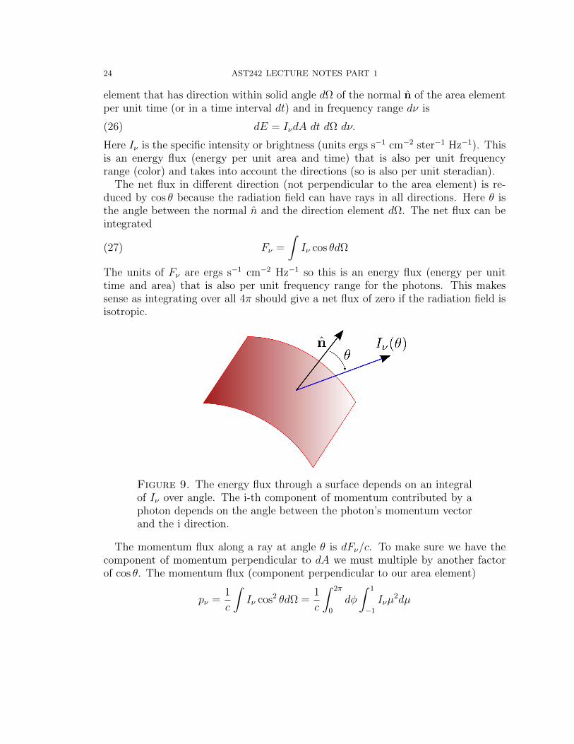
Consider an area element dA with normal n. We would like to know the energyand momentum flux through this element. We chose a coordinate system with anglesθ, φ oriented with respect to n. The energy of radiation crossing through the area dA


element that has direction within solid angle dΩ of the normal n of the area elementper unit time (or in a time interval dt) and in frequency range dν is

(26) dE = IνdA dt dΩ dν.

Here Iν is the specific intensity or brightness (units ergs s−1 cm−2 ster−1 Hz−1). Thisis an energy flux (energy per unit area and time) that is also per unit frequencyrange (color) and takes into account the directions (so is also per unit steradian).

The net flux in different direction (not perpendicular to the area element) is re-duced by cos θ because the radiation field can have rays in all directions. Here θ isthe angle between the normal n and the direction element dΩ. The net flux can beintegrated

(27) Fν =

∫Iν cos θdΩ

The units of Fν are ergs s−1 cm−2 Hz−1 so this is an energy flux (energy per unittime and area) that is also per unit frequency range for the photons. This makessense as integrating over all 4π should give a net flux of zero if the radiation field isisotropic.

Figure 9. The energy flux through a surface depends on an integralof Iν over angle. The i-th component of momentum contributed by aphoton depends on the angle between the photon’s momentum vectorand the i direction.

The momentum flux along a ray at angle θ is dFν/c. To make sure we have thecomponent of momentum perpendicular to dA we must multiple by another factorof cos θ. The momentum flux (component perpendicular to our area element)

pν =1

c

∫Iν cos2 θdΩ =

1

c

∫ 2π

0

dφ

∫ 1

−1Iνµ

2dµ


where µ = cos θ. If the radiation field is isotropic then Iν does not depend on θ and

pν =2π

c

∫ 1

−1Iνµ

2dµ =4π

3cIν

Now consider the surface of a star that is a black body. Integrating over ν andover 2π in directions we know that the net flux is

F = σBT4 =

∫ 1

0

2πIµdµ = πI

where I =∫Iνdν. The above equation implies that I = σBT

4/π. We can nowestimate the momentum flux in radiation assuming isotropic black body radiation

pr =4

3cσBT

4

This momentum flux is the flux of momentum through an area element with com-ponent perpendicular to the area element. Consequently it is part of the stress tensorπii but only contributes to a term that has two indexes the same (on the diagonal).This is why it can be considered as a pressure.

2.4. Conservation of Energy. Recall that from the first law of thermodynamicsthe internal energy per unit mass

De

Dt=DW

Dt+DQ

DT

where DWDt

is the work done per unit mass and DQDT

is the energy/heat gained per unitmass. We can rewrite the work

DW

Dt= −pD(1/ρ)

Dt=

p

ρ2Dρ

Dt

giving usDe

Dt=

p

ρ2Dρ

Dt− Qcool

where we have defined Qcool as a cooling rate, or the heat lost per unit mass and thisgives us the minus sign in the above equation.

Define a total energy per unit volume E

E ≡ ρ

(u2

2+ Φ + e

)Each term is recognizable as the kinetic energy per unit volume, the potential energyand the internal energy. For a fluid element expanding out the directional derivative

DE

Dt=u2

2

Dρ

Dt+ ρu · Du

Dt+ ρ

DΦ

Dt+ ρ

De

Dt+ (Φ + e)

Dρ

Dt


Our heat equation gives

TdS = de− p

ρ2dρ

If I set TdS equal to a cooling rate Q then we can write our conservation of energyequation as

DE

Dt=

[E

ρ+p

ρ

]Dρ

Dt− ρQ+ ρu · Du

Dt+ ρ

DΦ

Dt

Using some Lagrangian derivatives

E

ρ

Dρ

Dt= −E

ρρ∇ · u continuity/cons. mass

ρu · Du

Dt= ρu ·

[∂u

∂t+ u ·∇u

]Lagrang deriv.

= u · (−∇p− ρΦ) momentum cons.

ρDΦ

Dt= ρ

∂Φ

∂t+ ρu ·∇Φ Lagrange deriv.

p

ρ

Dρ

Dt= −p

ρρ∇ · u = −p∇ · u continuity

By combining the above with our equations for conservation of momentum, con-servation of mass and our definition for the directional derivative we can write con-servation of energy in the following form

(28)∂E

∂t+∇ · [(E + p)u] = −ρQcool + ρ

∂Φ

∂t

where Qcool is the heating cooling function, energy lost or gained per unit mass dueto heating and cooling with Qcool > 0 when cooling. The terms in the above relationshould make sense physically. The divergence term involving pu arrises from pdVwork.

Note we have taken care to keep in a term from heating and cooling, commonlyimportant in astrophysical settings. Here we have not taken into account dissipa-tive processes such as viscosity that would give a heat term dependent on velocitygradients. We have also not taken into account heat conductivity.

2.5. A polytropic gas and equations of state. A barytropic fluid is one where wecan form a relation p(ρ). In this case we need not use an additional energy equation(along with that for momentum and mass) but can determine the dynamics with theequations for conservation of momentum and mass alone alone with an equation ofstate. Baritropic flow is more general than isentropric flow and includes isothermalflow as well as a polytropic approximation.


A polytropic gas is an ideal gas with constant cP , cV , γ, and µ. The polytropicindex n (not necessarily an integer) is defined by γ = 1 + 1/n and

(29) p ∝ ρ1+1/n

Equipartition of energy with N degrees of freedom gives

(30) e =kBT

µmp

N

2= cV T

and so cV = kBµmp

N2

. Using the relations cP = cV + kB/(µmp) and γ = cP/cV we can

show that γ = 1+2/N . A popular value for γ is 5/3 corresponding to N = 3 degreesof freedom.

We can also show that the specific internal energy of a polytropic gas is

(31) e =p

(γ − 1)ρ

If the gas cools rapidly above a particular temperature then an isothermal equationof state can be adopted. This is often used for global simulations of molecular cloudsor the interstellar medium in galaxies.

(32) p = c2sρ

where cs is the sound speed.If the gas is polytropic and isentropic then

(33) p = Kργ

with constant K. The isentropic ideal gas has sound speed γP/ρ. Note that anisothermal fluid is also one with γ → 1.

An incompressible fluid is one where DρDt

= 0 and so ∇·u = 0. This approximationcan also be considered the limit γ →∞. A completely incompressible fluid will nottransmit sound waves.

2.6. The Lame-Enden equation. Taking a polytropic equation of state and hy-drostatic equilibrium, it is possible to solve for the density, potential and gravitationalpotential as a function of radius. The polytropic equation of state with index n

p = Kρ1+1n

Manipulating derivatives and using a derivative operator D

1

ρDp =

1

ρD(Kρ1+

1n

)= K(n+ 1)D

(ρ

1n

)Hydrostatic equilibrium is

−∂Φ

∂r=

1

ρ

∂p

∂r


Combing the previous two equations

dρ1/n

dΦ= − 1

K(n+ 1)

with solution

ρ1n = − Φ

K(n+ 1)+ constant

or

(34) ρ = ρc

(ΦT − Φ

ΦT − Φc

)nwith constants ρc,Φc the density and potential at the core and ρ = 0,ΦT the densityand potential at the surface. We define new variables

θ ≡ ΦT − Φ

ΦT − Φc

ξ =

(4πGρc

ΦT − Φc

)1/2

r(35)

where θ ranges from 0 at the surface to 1 at the core and ξ = 0 at the core. Poisson’sequation in spherical coordinates gives

(36)1

r2d

dr

(r2dΦ

dr

)= 4πGρ

Combining equations 34, 35, 36 gives

(37)1

ξ2d

dξ

(x2dθ

dξ

)= −θn

and this is known as the Lane-Emden equation. A boundary condition is dθdξ

= 0

at ξ = 0 corresponding to no gradient in potential energy at the core (no forceat the core). It is possible to solve the Lane-Emden equation analytically only forn = 0, 1, 5.

3. Microphysical Basis for Continuum Equations

3.1. The particle distribution function. To describe a distribution of particleswe can consider a particle distribution function that depends on position, velocityand time, f(x,v, t). Here f(x,v, t)dx3du3 represents the number of particles foundin a volume element of volume dx3 and in a velocity bin of size dv3 at time t. Thenumber density (number of particles per unit volume) at position x and at time twould be

n(x, t) =

∫ ∞−∞

f(x,v, t)d3v


where we perform the integral in 3 dimensions. If each particle has mass m then thedensity ρ(x, t) = mn(x, t). We can consider the average of any quantity Q as

〈Q〉 = n−1∫Qf(x,v, t)d3v

For example the bulk or average velocity would be

u = n−1∫

vf(x,v, t)d3v

and ∫vivjf(x,v, t)d3v = n〈vivj〉 for i 6= j

For a single component we can write∫v2i f(x,v, t)d3v = n〈v2i 〉

But this is not necessarily the same as nu2i which depends on the square of theaverage velocity. Usually

〈v2i 〉 6= u2i 〈vivj〉 6= uiuj

We can define a total velocity dispersion, σa, averaged over all directions, as

σ2a ≡

1

3

(〈(vx − ux)2〉+ 〈(vy − uy)2〉+ 〈(vz − uz)2〉

)=

1

3n

∫|v − u|2fd3v

Evaluating σ2a

σ2a =

1

3n

∫(v2 + u2 − 2u · v)d3v

=1

3(〈v2〉+ u2)− 2

3nu ·∫

vd3v

=1

3(〈v2〉+ u2)− 2

3u2

=1

3(〈v2〉 − u2)

so we can write

n〈v2〉 =

∫v2fd3f = n(u2 + 3σ2

a)

We can think about the velocity vi as a sum of the mean velocity ui plus a randomcomponent. Let

wij ≡ 〈(vi − ui)(vj − uj)〉 = 〈vivj〉 − uiuj


Here wij is a symmetric dispersion tensor with two indexes where each index canassume one of three values (x, y, z). When wij contains off diagonal components orits diagonal components are not equal we say the dispersion tensor is “anisotropic.”If the system is “isotropic” then the diagonal components would all be the same andthe off diagonal components would be zero.

We can write the trace of w as wii in summation notation and

σ2a =

1

3(〈v2〉 − u2) =

wii3

=1

3trace w

If wxx = wyy = wzz then σ2a = wxx. The dispersion tensor is symmetric. We can

decompose the dispersion tensor, wij, into the sum of a trace component that haszeros off the diagonal and a symmetric traceless component, yij;

yij =wij + wji

2− trace w

δij3

=wij + wji

2− σ2

aδij

Note that yij can contain components on the diagonal but their sum would be zero.If the system is isotropic then all components of yij would be zero.

We will associate pressure with the trace of wij or σ2a.

3.2. Boltzmann equation. In the absence of collisions the collisionless Boltzmannequation describes the evolution of the density distribution.

Df

Dt=∂f(x,v, t)

∂t+∂f(x,v, t)

∂x· dxdt

+∂f(x,v, t)

∂v· dvdt

= 0.

The derivative here is done with respect to all degrees of freedom of the distributionfunction. As v = dx/dt and dv/dt = −∇Φ for a force field with potential Φ we canwrite

(38)∂f(x,v, t)

∂t+ ∇xf(x,u, t) · v −∇vf(x,v, t) ·∇Φ = 0.

We have used gradient operators

∇x =

(∂

∂x,∂

∂y,∂

∂z

)∇v =

(∂

∂vx,∂

∂vy,∂

∂vz

)Below we often drop the x subscript on the spatial gradient operator. Equation 38is known as the collisionless Boltzmann equation. It is used to study the kinetictheory of gases, atomic nuclei and for stellar dynamical systems such as galaxies andglobular clusters. The collisionless Boltzmann equation is sufficiently complex thatit is usually difficult to solve. Equation 38 is sometimes written

Df

Dt= 0


where the Lagrangian derivative is

D

Dt=

∂

∂t+ v ·∇x −∇Φ ·∇v

Here the Lagrangian derivative describes a small element moving in phase space or(x,v). Previously we used a Lagrangian derivative for a small element moving onlyin Cartesian space.

When collisions are important we can use the full Boltzmann equation by addinga source term that is due to collisions

Df

Dt=

(∂f

∂t

)C

where the term on the right hand side depends on the cross sections of particles andtheir velocity differences. In many situations collisions conserve mass, momentumand kinetic energy. When these are conserved∫

m

(∂f

∂t

)C

d3v = 0∫mv

(∂f

∂t

)C

d3v = 0∫mv2

(∂f

∂t

)C

d3v = 0

3.3. Conservation of mass. The simplest continuum equation can be made byintegrating the Boltzmann equation over all possible velocities. The first term givesus the time derivative of the particle density as shown in the previous equation.Integrating the first term in the collisionless Boltzmann equation∫ ∞

−∞

∂f(x,v, t)

∂td3v ≈ ∂

∂tn(x, t)

As derivatives with x and v commute we can integrate the second term in thefollowing way ∫ ∞

−∞∇f(x,v, t) · v d3v = ∇ ·

∫fvd3v = ∇ · (nu)

where we have rewritten the last term in terms of the average velocity u. The lastterm in the collisionless Boltzmann equation

−∫

∇vf(x,v, t) ·∇Φd3v


we can integrate and write in terms of f at infinity and so will be zero. Putting thesetogether with the integral of the collision term (also zero) we find

∂n

∂t+ ∇ · (nu) = 0

To summarize: the integral over velocity space of the Boltzmann equation gives anequation that looks just like the equation for conservation of mass for a fluid.

3.4. Conservation of momentum. To derive an equation similar to Euler’s equa-tion (conservation of momentum) we multiply the Boltzmann equation by v andthen again integrate over velocity space. Taking the i-the component of the velocityand using summation notation for the other indices

(39)

∫ (∂f

∂tvi +

∂f

∂xjvjvi −

∂f

∂vj

∂Φ

∂xjvi

)d3v =

∫ (∂f

∂t

)C

d3v = 0

Consider the first term∫∂f

∂tvid

3v =∂

∂t

∫fvid

3v =∂(nvi)

∂t

Consider the second term of equation 39. This can be written∫∂f

∂xjvjvid

3v =∂

∂xj[n〈vjvi〉]

We can decompose this in terms of the dispersion tensor (w) and then the tracelesscomponent of the dispersion tensor (y) and the average dispersion (σ2

a)

∂

∂xj[n〈vjvi〉] =

∂

∂xj[n(uiuj + wij)]

=∂

∂xj[n(uiuj + σ2

aδij + yij)]

=∂

∂xj[n(uiuj + yij) + Pδij]

where we define a pressure in terms of the trace of the dispersion tensor

P ≡ nσ2a =

nwii3.

Altogether the second term in the momentum equation (39) becomes

∂

∂xj(nuiuj + Pδij + nyij)

We recognize the first two terms inside the derivative, nuiuj +Pδij as resembling thestress tensor. The last term nyij depends in the traceless component of the dispersiontensor and is only non-zero when the velocity distribution is anisotropic.


The third term in the momentum equation (39) requires us to evaluate

∂Φ

∂xj

∫∂f

∂vjvi d

3v =∂Φ

∂xjδij

∫ ∫(fvi|∞−∞ −

∫fdvi)dvkdvl

= −n ∂Φ

∂xjδij = −n ∂Φ

∂xi

We integrate the integral by parts finding a non-zero term unless i = j. So the thirdterm in equation 39 becomes

+n∂Φ

∂xiAltogether our equation for conservation of momentum becomes

∂

∂t(nui) +

∂

∂xj(nuiuj + Pδij + nyij) + n

∂Φ

∂xi= 0

This is familiar! Except for the term associated with anisotropy this looks just likeour relation for conservation of momentum in conservation law form.

By making use of the equation of continuity we can manipulate this equation sothat it becomes a force equation that resembles Euler’s equation

Du

Dt= − 1

n∇P −∇Φ− 1

n∇ · (ny)

where the last term is a divergence of the traceless component of the dispersion tensor.If the velocity dispersion is isotropic then y = 0 and we recover Euler’s equation. Tosummarize: by multiplying the Boltzmann equation by velocity and integrating overall velocities we recover an equation that looks remarkably like Euler’s equation.

Here we have integrated over velocity. If one integrates over all space insteadone can derive tensor “virial” equations. Integrating only over velocity and workingin cylindrical or spherical coordinates the equations, and in the setting of stellardynamics, the equations are called the Jeans equations.

3.5. Validity of continuum fluid approximation. When collisions are frequentwe expect the distribution function to become Maxwellian. A crude approximationknown as the BGK approximation for the collision term that approximates thiscondition is

(40)

(∂f

∂t

)c

≈ −1

τ(f − fM)

where fM is a Maxwellian distribution that has the same n, u and velocity dispersionas f . The timescale τ is known as the relaxation time. We expect τ to be approxi-mately the mean free flight time. The continuum or fluid approximation is good ifthe collision time dominates and so characteristic timescales are longer than τ . Anequivalent way to describe this is to require that the mean free path, λ be smaller


than the characteristic lengthscale L or λ L. The mean free flight time and meanfree path are related by λ ∼ στ where σ is the velocity dispersion.

Above we have used a distribution function to show that moments of the dis-tribution function look similar to equations describing conservation of mass andmomentum for a fluid. When collisions are taken into account in a more detailedway dissipative or non-conservative processes can be modeled such as viscosity andtransport effects such as heat conduction.

4. Summation notation, the permutation tensor and some indexgymnastics

We will often be manipulating vectors in this class, so it will be useful to speedup calculations with summation notation and using a permutation tensor εijk. Thetensor εijk is known as the Levi-Civita tensor or the permutation tensor and is

(41) εijk ≡

1−1

0for

ijk is an even permutationijk is an odd permuationtwo or more of ijk are equal

Each of ijk is a coordinate like xyz. For example εxyz = 1 however εxzy = −1.Consider the cross product of two vectors

(42) C = A×B

The iith component of C can be written

Ci = εijkAjBk

and we have implicitly summed over all indices that appear twice in the equation.Here the indices j, k appear twice in the equation and so are summed over all coor-dinates, xyz. The Levi-Civita tensor is zero unless all indices differ. Each Ci can bewritten as a sum of two terms one with positive sign corresponding to the even per-mutation and the other with a negative sign corresponding to the odd permutation.

Using summation notation

(43) ∇ ·A =∂Ai∂xi

and we have implicitly summed over i. Here xx represents x and xy gives y and xzgives z. Alternatively one can let ijk range from 1-3 and let A1 = Ax, A2 = Ay,A3 = Az,

∂∂x1

= ∂∂x

, ∂∂x2

= ∂∂y

, ... etc.

The expression δij is the Kronecker delta which is a discrete version of the deltafunction.

(44) δij ≡

10

fori = ji 6= j


When there are expressions with the Levi-Civita tensor it is often useful to use therelation

(45) εijkεilm = δjlδkm − δjmδklOnce you notice the patterns in the indices it is not hard to remember the relation.

In computations, it is useful to remember that indices in the Levi-Civita tensorcan be rotated

εijk = εjki = εkij

while maintaining the same sign in the permeation. Any two indices can be flipped

εijk = −εjikand reversing the sign.

Let us prove a vector identity that we will use in the next lecture.Example: Prove the vector identity using summation notation

(u · ∇)u = ∇(u2

2

)− u× (∇× u)

The i-th component for the expression on the right

uj∂uj∂xi− εijkujεklm

∂um∂xl

= uj∂uj∂xi− εkijεklmuj

∂um∂xl

= uj∂uj∂xi− (δilδjm − δjlδim)uj

∂um∂xl

= uj∂ui∂xi− uj

∂uj∂xi

+ uj∂ui∂xj

= uj∂ui∂xj

This is the i-th component for the expression on the left (u · ∇)u. We have provedthe identity.

5. Extremely Short Introduction to Relativistic Hydrodynamics

To make sure expressions are relativistically invariant (under Lorenz transforma-tions or boosted frame of reference) it is desirable to work with 4 vectors. In aparticular reference frame the 4 momentum of a massive particle or photon

(46) P = (E,p)

where E is the energy and p is the momentum (a three dimensional vector).From here we set the speed of light c = 1. A pseudo metric is

(47) ds2 = −dt2 + dx2 + dy2 + dz2 = gµνdxµdxν


with

(48) g00 = −1 g11 = g22 = g33 = 1 gij,i6=j = 0

The metric gives a Minkowski norm

(49) |P|2 = gµνPµP ν

The norm |P|2 = −m2 for a massive particle and 0 for a photon.A particle with mass m, that is moving with velocity v with respect to an observer

has four-momentum (as seen by the observer)

(50) P = (γm, γβm)

where γ = (1 − β2)−1/2 and β = v/c with v the velocity in three dimensions. Torestore units multiply the energy by c2 and the momentum by c. Either the spaceor time parts of the metric then gain a factor of c2.

A Lorenz boost transforms four-vectors

(51) Λ(β) =

γ −γβ1 −γβ2 −γβ3−γβ1 (γ − 1)

β21

β2+ 1 (γ − 1)

β1β2β2

(γ − 1)β1β3β2

−γβ2 (γ − 1)β2β1β2

(γ − 1)β22

β2+ 1 (γ − 1)

β2β3β2

−γβ3 (γ − 1)β3β1β2

(γ − 1)β3β2β2

(γ − 1)β23

β2+ 1

from one relativistic coordinate frame to another. Here β = (β1, β2, β3). Lorenzboosts conserve the Minkowski norm.

A particle or an observer can be described by a 4-velocity u. In the observer’sframe, he or she is not moving so the 4-velocity u = (1, 0, 0, 0). The norm |u|2 = −1.In a different frame u = (γ, γβ). The first component of u describes time dilation,or how time advances in the observer’s frame compared to the reference frame inwhich the 4-vector is written. u0 = dt

dτrelating world time to proper time. For

hydrodynamics a relevant quantity is the velocity of a fluid element. We describethis with a 4-velocity u.

Baryon conservation can be written with 4-vectors

(52) ∇ · (nu) = 0 or (nui),i = 0

where n is the number of baryons per unit volume. In an observer frame u = (γ, γβ)which in the non-relativistic limit is u → (1,v) with v the three-vector velocity.Inserting this into above relation we find

(53)∂n

∂t+ ∇ · (nv) = 0


where the divergence is in three-dimensions. This looks like a normal conservationlaw, giving us some confidence that the relativistic version is correct.

The condition for adiabatic motions in terms of the 4-velocity is similar

(54) ∇ · (su) = 0 or (sui),i = 0

where s is the entropy per unit volume.In the frame moving with the fluid the energy momentum tensor or stress-

energy tensor is

(55) T =

e 0 0 00 p 0 00 0 p 00 0 0 p

with p the pressure and e the energy density. Ignoring internal degrees of freedomand photons e = ρc2. The T 00 component gives the energy density, and the otherdiagonal components, T xx, T yy, T zz, the momentum flux or the pressure.

In another coordinate system, the stress energy tensor (for an ideal fluid) is moregenerally

(56) T = (e+ p)u⊗ u + pg

with g the metric tensor with g00 = −1, g11 = g22 = g33 = 1 and gij,i6=j = 0. Recallthat u is the flow four vector of the fluid. Using indices of the four vector u

(57) T ij = (e+ p)uiuj + pgij,

or if we lower indices with the metric tensor

(58) Tij = (e+ p)uiuj + pgij.

Here components T 0i or T i0 with i > 0 describe energy flux or momentum density.The components T ij with i, j > 0 describe components of momentum flux, as wastrue when we worked with the stress tensor. We can compare the stress-energy tensorto the stress tensor we previously used in the non-relativistic limit

(59) π = pg + ρu⊗ u

where u is only a 3-vector. The two tensors are similar in form, and that’s comforting.The stress energy tensor is a tensor with two indices. Each index of a tensor

transfers separately during a coordinate transformation. Here the coordinate trans-formation is the Lorenz boost.

(60) T ij = T klΛikΛ

jl

Using a Lorenz boost we can transform equation 55 into equation 56.


The 4-momentum is conserved, giving rise to four conservation laws. Conservationof energy and momentum is equivalent to

(61) T ij,j = 0

Writing this out

(62)∂T i0

∂x0+∂T i1

∂x1+∂T i2

∂x2+∂T i3

∂x3= 0

or

(63)∂T it

∂t+∂T ix

∂x+∂T iy

∂y+∂T iz

∂z= 0

for each index i.

6. Acknowledgements

These lecture notes are loosely based on Shu’s book Gas Dynamics, lecture notesby Gordon Ogilvie and Cathy Clarke’s and Carswell’s book on Astrophysical Fluiddynamics. For relativistic hydrodynamics Landau and Lifshitz or Misner, Thorneand Wheeler.

Documents

AST242 LECTURE NOTES PART 1 Contentsastro.pas.rochester.edu/~aquillen/ast242/lecturenotes1.pdf · 4 AST242 LECTURE NOTES PART 1 Figure 2. Streamlines, paths and streaks. Another example