Assortative Matching of Exporters and Importers

Yoichi Sugita

SSE

Kensuke Teshima

ITAM

Enrique Seira

ITAM

Preliminary and Incomplete

First Draft: November 2013

Abstract: This paper examines what determines matching of exporters and importers. Both exporters

and importers concentrate more than 80% of product-level trade volume on trade with the largest

partner firm in Mexican textile/apparel exports to the US. Motivated by this new fact, we develop a

one-to-one matching model of exporters and importers where the complementarity/substitutability of

capability (productivity/quality) within matches determines the sign of sorting in matching. Increases

in Chinese exporters to the US at the end of the Multi-Fiber Arrangement in 2005 caused Mexican

exporters to downgrade and US importers to upgrade their main partners. This pattern is consistent

with complementary-driven positive assortative matching, but not with capability-independent random

matching or substitutability-driven negative assortative matching. Our finding suggests trade liberal-

ization improves matching of firms in global supply chains as a part of within industry reallocation that

improves the aggregate industrial performance.

Keywords: Firm heterogeneity, assortative matching, two-sided heterogeneity, trade liberalization

Acknowledgments: We thank Secretaría de Economía of Mexíco and the Banco de Mexíco for helpwith the data. Financial supports from the Private Enterprise Development in Low-Income Countries(PEDL) and the Wallander Foundation are gratefully acknowledged. Francisco Carrera, Diego de laFuente and Carlos Segura provided excellent research assistance.

Author: Yoichi Sugita, Stockholm School of Economics, Department of Economics, Box 6501, 11383Stockholm, Sweden (E-mail: yoichi.sugita@hhs.se, Tel: +46-8-7369254, Fax: +46-8-313207).

Author: Kensuke Teshima, Centro de Investigación Económica, Instituto Tecnológico Autónomo deMéxico Av. Santa Teresa # 930, México, D. F. 10700 (E-mail: kensuke.teshima@itam.mx)

Author: Enrique Seira, Centro de Investigación Económica, Instituto Tecnológico Autónomo deMéxico Av. Santa Teresa # 930, México, D. F. 10700 +52(55) 56284000 ext 6776 E-mail: en-rique.seira@itam.mx

1 Introduction

The last decade has witnessed a rise in research in heterogeneous firms and trade. A robust finding that

firms with relatively high productivity/quality (capability) participate in exporting and/or importing

within industries (e.g. Bernard and Jensen, 1995, 1999) has developed new theories emphasizing

within industry reallocation by trade (Melitz, 2003; Bernard, Eaton, Jensen, and Kortum, 2003): trade

improves aggregate industrial performance by shifting production factors to more capable firms within

industries as empirical studies observed (e.g. Pavcnik, 2002). This new reallocation mechanims have

been applied for various issues and centered in the trade research of the last decade.1

In contrast to the level of our knowledge about which firms participate in trade, we know little about

which exporters trade with which importers, i.e. matching of exporters and importers. Do exporters

and importers match based systematically on any firm characteristics? Do trade liberalization change

matching of exporters and importers in any systematic way? This paper is one of the first attempts to

answer these questions empirically.

Workhorse trade models consider types of international trade where matching of exporters and

importers is not important. Perfectly competitive models such as the Ricardo and Heckscher-Ohlin

models do not predict any systematic matching pattern because in equilibrium exporters and importers

are indifferent on whom they trade with.2 The love of variety model also abstracts away from matching,

predicting that all exporters trade with all importers.

Data suggests matching is important at least for some industries. In our customs transaction data

set of Mexican textile/apparel exports to the US, we are able to observe the identities of exporters

and importers at transaction level. Table 1 presents a striking fact on matching: a one-to-one matching

model is a good approximation for markets of HS 6 digit textile/apparel products. Each column in Table

1 reports the volume share of a type of trade in the total export volume for Mexico’s Textile/Apparel

(HS50-63) exports to the US. The “One to One” column reports the share of trade in which both the

exporter and the importer are the only partners of each other in a given product-year combination.

Trade between one-to-one relationship accounts for around 28% of textile/apparel trade. Furthermore,

even firms trading with multiple partners conduct most of their product-level trade with a single partner.1See survey papers e.g. Bernard, Jensen, Redding, and Schott (2007; 2012) and Redding (2011) for more papers in the

literature.2Because of this prediction, perfectly competitive models are sometimes called “anonymous market” models.

1

For each product-year combination, we identify the “main partner” of each firm, with whom the firm

makes the largest trade volume. The “Main to Main” column reports the share of trade in which the

exporter is the main partner of the importer and at the same time the importer is the main partner of

the exporter. The column shows that trade within one-to-one matches of the main partners accounts

for 80% of textile/apparel trade volume.3 This huge share of trade between the main partners suggests

that understanding matching of the main partners is important for better understanding of international

trade.

Year One to One Main to Main Main2 to Main22004 0.32 0.77 0.922005 0.29 0.79 0.922006 0.25 0.80 0.942007 0.28 0.81 0.932008 0.26 0.78 0.94

Note: Each column reports the volume share of a type of transactions in the totalexport volume for Mexico’s Textile/Apparel (HS50-63) exports to the US. In a “Oneto One” transaction, the exporter and the importer trade in the product only with eachother; in a “Main to Main” transaction, the exporter and the importer trade in theproduct by the largest volume with each other; In a “Main2 to Main2” transaction,the exporter and the importer trade in the product by the largest or the second largestvolumes with each other. Data cover transaction from June to December for 2004 andfrom January to December for other years. See section 4 for the data source.

Table 1: Shares of trade volume with the Main Partners in Mexico’s Textile/Apparel exports to the US

Motivated by Table 1, we analyze the determinants of matching of the main partners in Mexico’s

Textile/Apparel exports to the US in light of a one-to-one matching model of exporters and importers.

Our base model is Sugita (2013) who developed a Becker (1973) type positive assortative matching

model of quality-differentiated exporters and importers and integrated it to a standard Melitz type

model. To guide our empirical exercise, we extend the Sugita (2013) model to allow for more general

sorting patterns and consider the heterogeneity in firm’s “capability” nesting two types of firm het-

erogeneity considered in productivity (e.g. Melitz, 2003) and in quality (e.g. Baldwin and Harrigan,

2010; Johnson, 2012). Suppliers (exporters) and final producers (importers) are both heterogeneous3We identify the second main partner for each firm with whom the firm makes the second largest trade volume for a given

product-year combination. The “Main2 to Main2” column in Table 2 reports the share of trade in which the exporter is themain partner or the second main partner of the importer and the importer is the main partner or the second main partner ofthe exporter.

2

in capability and match in one-to-one to form global supply chains under perfect information. As

well known from classic matching models (e.g. Becker, 1973), the interaction of capabilities within

matches determines the sign of sorting in matching. If capabilities are complement, a positive assor-

tative matching (PAM) holds that firms match with those with similar capabilities. If capabilities are

substitute, a negative assortative matching (NAM) holds that firms with high capability match with

those with low capability. If capabilities are independent, matching patterns are not determined and

firms match randomly.

The model demonstrates the importance of identifying the sorting in matching of exporters and

importers in two respects. First, if matching is systematically determined by complementarity or sub-

stitutability of firms, trade liberalization may improve matching of firms in global supply chains as a

part of within industry reallocation that improves the aggregate industrial performance as Antras, Gar-

icano, and Rossi-Hansberg (2006) and Sugita (2013) demonstrated in their models exhibiting PAM.

Second, the sign of sorting and the existence of importer heterogeneity may affect the measurement of

firm’s performance in empirical research. Our model is suitable for analyzing this question since the

model nests standard models of heterogeneous exporters with no importer heterogeneity as a special

case. We consider a conventional measure of productivity, revenue productivity, as an example. We

found that the existence of importer heterogeneity affects revenue productivity of exporters and that

the direction of the effect is the opposite between the case of PAM and the case of NAM.

Finally, we empirically identify the sign of sorting exploiting a large scale and arguably exogenous

trade liberalization episode, the end of the Multi-Fiber Arrangement (MFA) in 2005. Before 2005

Mexican exporters had already acquired free access to the US market through the North American

Free Trade Agreement and enjoyed the advantage over exporters from other countries that faced se-

vere quota restrictions to the US market. In 2005 when the US removed quota restrictions, there was

a surge in imports in the US apparel/textile market mostly due to the new entry of Chinese exporters

(Brambilla, Khandelwal, and Schott, 2010; Khandelwal, Schott, and Wei, 2013). As a result of this,

Mexican exporters faced an increase in competition with Chinese exporters in the US market. If the

matching of Mexican exporters and US importers were positive assortative due to the complementarity

of capabilities, after the end of the MFA we should observe the following change. Some US im-

porters terminate trade with Mexican exporters to import form Chinese exporters.Mexican exporters

3

are forced to switch to US importers with lower capability than their previous partners. This means

that US importers who continue to imports from Mexico now can trade with Mexican exporters with

higher capability than their previous partners. Using firm’s trade volume in 2004 as a proxy for firm’s

capability, we create a ranking of Mexican exporters and a ranking of US importers and investigate

the difference in the rank of the main partner in 2004 and the rank of the main partner in 2007 for

Mexican exporters and US importers. We found a strong support for the above prediction of comple-

mentary driven positive assortative matching. Namely, Mexican exporters downgraded US importers

and US importers upgraded Mexican importers more often in industries liberalized in 2005 than in

industries already liberalized before 2005. Furthermore, we found no other systematic pattern of part-

ner changes, which rejects the capability independent random matching and the substitutability driven

negative assortative matching.

Our finding provides the first support for complementarity-driven assortative matching in Antras et

al. (2006) and Sugita (2003). The systematic change in matching we observed suggests that trade lib-

eralization improves matching of firms in global supply chains as a part of within industry reallocation

that improves the aggregate industrial performance.

Related Literature

Our paper is related to the growing literature on importer-exporter matched transaction data. As pio-

neering studies on the static characteristics of matching of exporters and importers, Blume, Claro, and

Horstmann (2011, 2012) and Eaton, Eslava, Jinkins, Krizan, and Tybout (2012) studied trade between

two countries, Chile-Colombia trade, Argentina-Chile trade, and Colombia-US trade, respectively.

Bernard, Moxnes, and Ulltveit-Moe (2013) and Carballo, Ottaviano, and Volpe Martincus (2013) stud-

ied exports from one country to multiple destinations in Norwegian customs data and in the customs

data of Costa Rica, Ecuador, and Uruguay, respectively. These studies typically decompose firm’s

exports into extensive margins and intensive margins, extending the method of Eaton, Kortum and

Kramartz (2010), to include the number of buyers as another extensive margin and investigate how the

difference in the number of buyers explains the difference in export volumes across exporters.

Our focus is different from these studies in several points. First, while these studies define a match

of an exporter and an importer at destination-year level, we define a match more narrowly at product-

4

destination-year level. Second, motivated by Table 1, our main interest is in the determinant of match-

ing between the main partners, which was not studied in the above mentioned papers. Third, while

these studies analyze matching at one point of time, our main focus is on the response of matching to

a specific type of shock.

Those transaction data sets that these studies and our study used do not contain financial infor-

mation of exporters and importers for the estimation of capability. Our contribution is to develop a

methodology for identifying the sign of sorting in matching without estimating capability.

Regarding dynamic characteristics of matching, Machiavello (2010) and Eaton et al. (2012) are

pioneering studies on how new exporters acquire or change buyers in Chilean exports of wine to the

UK and in Colombian exports to the US. While these two studies consider steady state dynamics, we

focus on how matching responds to a specific shock to a market.

Our theoretical part rests on positive assortative matching models of exporters and importers de-

veloped by Antras, Garicano, and Rossi-Hansberg (2006) and Sugita (2013).4 Antras et al. (2006)

and Sugita (2013) differ in the source of the heterogeneity of production teams (firms). In Antras

et al. (2006), firms are heterogeneous in the skills of workers and technology is identical; in Sugita

(2013), firms are heterogeneous in technology but workers are homogeneous.5 Our finding supports

for positive assortative matching Antras et al. (2006) and Sugita (2013) though we need to work further

to distinguish the two models. Our theoretical contribution is to extend Sugita (2013) in two points.

First, the model introduce firm heterogeneity in capability, which nests firm heterogeneity in produc-

tivity and quality. Second, the model allows for the cases of negative assortative matching and random

matching to derive predictions that can be used for identifying the sign of sorting from data.4The trade literature has also developed other matching models. The early models analyze random matching of symmetric

and horizontally differentiated exporters and importers (Casella and Rauch, 2001; Rauch and Casella, 2003; Rauch andTrindade, 2003; Grossman and Helpman, 2005).

5The difference between Sugita (2013) and Antras et al. (2006) is reminiscent of the difference between Melitz (2003)and Yeaple (2005).

5

2 Theoretical Framework

2.1 A Matching Model of Global Supply Chains

We consider a partial equilibrium model of global supply chains producing differentiated goods. Our

model is a partial equilibrium version of Sugita (2010; 2013), but consider three countries and more

general sorting patterns.6 The production involves three countries, Mexico, China, and the US. There

are two types of firms, final producers and intermediate goods suppliers (suppliers). Suppliers in Mex-

ico and in China export intermediate goods to the US. Final producers in the US import intermediate

goods, produce differentiated final goods, and sell them in the US market. At this moment, no trade

barrier is imposed on exports from Mexico or China.

The representative consumer in the US maximizes the following utility function:

U =

�

⇢

lnˆ

!2⌦✓(!)

↵

q(!)

⇢

d!

�+ q0 s.t.

ˆ!2⌦

p(!)q(!)d! + q0 = I.

where ⌦ is a set of available differentiated final goods, ! is a variety of differentiate final goods,

p (!) is a price of !, q(!) is consumption of !, q0 is consumption of a numeraire good, and I is an

exogenously given income. Parameter � captures industry-wide demand shocks. Parameter ✓(!) is

“capability” of the producer of ! and ↵ � 0 determines the interpretation of capability. When ↵ > 0,

capability ✓ expresses quality as a positive demand shifter. Consumer’s demand for a variety with price

p and capability ✓ is derived as q(p, ✓) = �P

��1(p/✓

↵

)

��, where � ⌘ 1/ (1� ⇢) > 1 is the elasticity

of substitution and P ⌘⇥´

!2⌦ p(!)

1��

✓ (!)

↵�

d!

⇤1/(1��) is a price index.

Firms are heterogeneous in their own capability. Capability expresses either productivity or quality,

depending on other parameters in the model.7 Let x and y be the capability of suppliers and final

producers, respectively. There are mass M

M

of suppliers in Mexico, MC

of suppliers in China and

M

U

of final producers in the US. For simplicity, a Chinese supplier is a perfect substitute for a Mexican

supplier with the same capability. The capability of Mexican suppliers and that of Chinese suppliers6Sugita (2013) integrates a positive assortative matching model of quality-differentiated final producers and suppliers

with Melitz (2003) type of heterogeneous firms with endogenous entry and a Ricardian comparative advantage model ofglobal supply chains. Our model is more similar to Sugita (2013)’s old version, Sugita (2010). The main difference betweenSugita (2010) and Sugita (2013) is that the former uses a CES utility function and the latter uses a quadratic utility function.

7The heterogeneous firm trade literature has considered two types of firm heterogeneity, productivity and quality. Weborrow the term “capability” from Sutton (2007).

6

also follow an identical distribution and the c.d.f. is given by F (x). The c.d.f. for the capability of the

US final producers is given by G(y).

Final goods are produced in team. A final producer and a supplier form a team to produce one

variety of final goods. Once teams are formed, suppliers tailor intermediate goods for a particular

variety of final goods; therefore, firms transact intermediate goods only within their team. Each firm

joins only one team.

We introduce the capability of a team ✓ and assume ✓(x, y) is an increasing function of capabilities

of team members, ✓x

⌘ @✓/@x � 0 and ✓

y

⌘ @✓/@y � 0. The cross partial derivative ✓

xy

⌘

@

2✓/@x@y expresses the complementarity or substitutability of capabilities within teams. Throughout

the paper, we focus on the following three cases that generate sharp predictions on matching patterns:

(1) Case-C (Complement) ✓xy

> 0 (✓ is strict supermodular) for all x and y; (2) Case-I (Independent)

✓

xy

= 0 (✓ is additive separable) for all x and y; (3) Case-S (Substitute) ✓

xy

< 0 (✓ is strict sub

modular) for all x and y. Both Case-C and Case-S (and the intermediate Case-I) are theoretically

plausible (e.g. Grossman and Maggi, 2000). An example for Case-C is the complementarity of quality

of tasks in a production process (Kremer, 1993; Kugler and Verhoogen, 2012; Sugita, 2013). For

instance, a high quality car part is more useful when it is combined with other high quality car parts.

An example for Case-S is technological spillovers through learning and teaching. Gains from learning

from high capable partners might be greater for low capable firms.

Production technology is of Leontief type. When a team produces q units of final goods, the

supplier in the team produces q unit of intermediate goods with costs c

x

✓

�

q + f

x

; then, using them,

the final producer assemble final goods with costs cy

✓

�

q + f

y

. Team’s total costs are c✓

�

q + f , where

c ⌘ c

x

+ c

y

and f ⌘ f

x

+ f

y

. Parameter � determines the interpretation of capability. Capability

expresses quality when � > 0 and productivity when � < 0. The marginal cost of each firm is assumed

to depend on team’s capability. This assumption is mainly for simplicity, but it also aims to express

externality within teams that makes marginal costs to depend on partner’s capability as well as its

own.8

The model has two stages. In Stage 1, final producers and suppliers form teams under perfect8One example for this is that producing high quality final goods need extra costs of quality control at each production

stage because even one defective component can destroy the whole product (Kremer, 1993). Another example is productivityspillovers through teaching and learning within a team.

7

information. After teams are formed, in stage 2, teams compete in the US final good market in a

monopolistically competitive fashion.

Stage 2 We obtain an equilibrium by backward induction. Team’s optimal price is p(✓) = c✓

�

/⇢.

Hence, team’s revenue R(✓), total costs C(✓), and joint profits ⇧ (✓) are

R(✓) = �A✓

�

, C(✓) = (� � 1)A✓

�

+ f, and ⇧ (✓) = A✓

� � f,

where A ⌘ �

�

⇣⇢P

c

⌘��1

. Parameter � ⌘ �+(↵��)� summarizes how capability affects demand and

costs. When � = 1, the sign of the cross derivative of joint profits @2⇧/@x@y is equal to the sign of

✓

xy

. We assume � = 1 in the following to simplify expositions.9

Stage 1 Firms choose their partners, taking A as given. Since no resale of intermediate goods is

possible, each supplier charges a non-linear price (payment per match) instead of a conventional linear

price (payment per good). The payment between a final producer and a supplier is endogenously

determined so as to make matching stable. Profit schedules, ⇡x

(x) and ⇡

y

(y), and matching functions,

m

x

(x) and m

y

(y), characterize equilibrium matching. A supplier with capability x matches with

a final producer with capability m

x

(x) and receives the residual profit ⇡x

(x) after paying profits

⇡

y

(m

x

(x)) for the partner. A function m

y

(y) is the inverse function of mx

(x) such that mx

(m

y

(y)) =

y. We focus on stable matching that satisfies two conditions: (i) (individual rationality) all firms earn

non-negative profit, ⇡x

(x) � 0 and ⇡

y

(y) � 0 for all x and y; (ii) (pair-wise stability) each firm is the

optimal partner for the other team member:

⇡

x

(x) = A✓(x,m

x

(x))� ⇡

y

(m

x

(x))� f = max

y

A✓ (x, y)� ⇡

y

(y)� f

⇡

y

(y) = A✓(m

y

(y), y)� ⇡

x

(m

y

(y))� f = max

x

A✓ (x, y)� ⇡

x

(x)� f.

9The cross derivative of joint profits becomes

⇧xy

⌘ @

2⇧ (✓ (x, y))@x@y

= �A✓

��1

✓

xy

+ (� � 1)✓

y

✓

�.

Therefore, the sign of ⇧xy

is equal to the sign of ✓xy

if � = 1. If � > 1, there is a possibility that ⇧xy

> 0 and ✓

xy

0hold; if � < 1, there is a possibility that ⇧

xy

< 0 and ✓

xy

� 0.

8

The first order conditions become

⇡

0x

(x) = A✓

x

(x,m

x

(x)) and ⇡

0y

(y) = A✓

y

(m

y

(y), y) (1)

and prove that profit schedules are increasing in capability. Because of fixed costs, final goods with

the lowest quality ✓

L

are not sold on the market. There are quality cutoffs x

L

and y

L

such that only

final producers with x � x

L

and suppliers with y � y

L

participate in the matching market, i.e. in

international trade. These cutoffs satisfy

⇡

x

(x

L

) = ⇡

y

(y

L

) = 0 and (M

M

+M

C

) [1� F (x

L

)] = M

U

[1�G(y

L

)] . (2)

The second condition in (2) expresses the mass of suppliers in the matching market is equal to that of

final producers.

Integrating the first order conditions (1) with initial conditions (2), we obtain profit schedules as

⇡

x

(x) = A

ˆx

x

L

✓

x

(t,m

x

(t))dt and ⇡

y

(y) = A

ˆy

y

L

✓

y

(m

y

(t), t)dt.

The export volume X(x) and the total costs Cx

(x) of a supplier depend on its capability as well as that

of the partner:

X(x) = C

x

(x) + ⇡

x

(x) and C

x

(x) =

c

x

c

(� � 1)A✓(x,m(x)) + f

X

. (3)

It is known that the sign of the cross derivative of team’s joint payoff, which corresponds to the sign

of ✓xy

, determines the sign of sorting in stable matching in a frictionless one-to-one matching model

(e.g. Becker, 1973). In Case-C, we have positive assortative matching (PAM) (m0x

(x) > 0): high

quality firms match high quality firms while low quality firms match low quality firms. In Case-S, we

have negative assortative matching (NAM) (m0x

(x) < 0): high quality firms match low quality firms.

In Case-I, we cannot determine a matching pattern (mx

(x) cannot be defined as a function) since each

firm is indifferent about partner’s capability. Therefore, we assume matching is random in Case-I. A

formal proof for these results is given in Appendix.

9

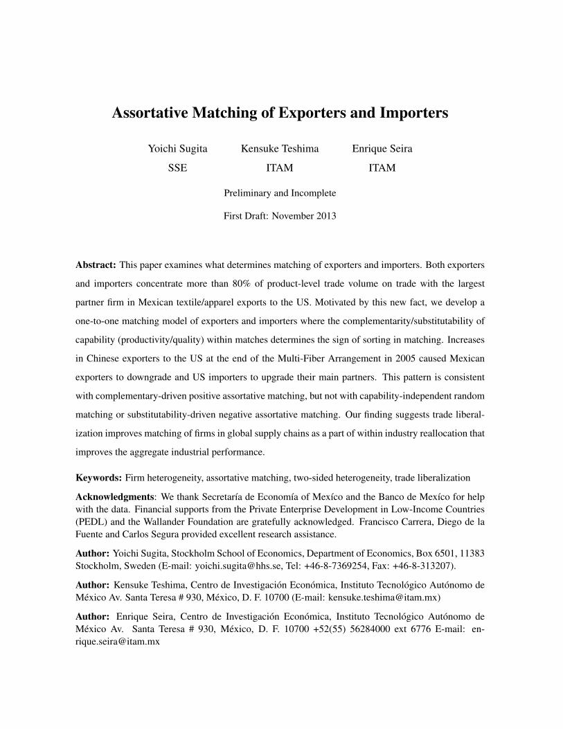
In Case-C, matching functions mx

(x) satisfies the following “matching market clearing” condition.

(Case-C) (M

M

+M

C

) [1� F (x)] = M

U

[1�G (m

x

(x))] for all x � x

L

, (4)

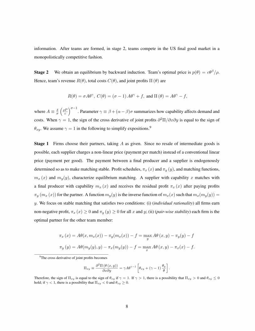
The left hand side of (4) is the mass of suppliers that have higher capability than x and the right hand

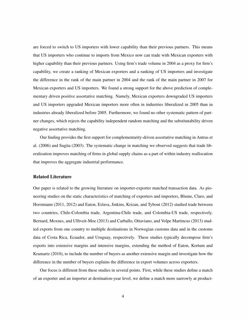
side is the mass of final producers who match with them. Figure 1 describes the matching market

clearing condition (4). Each rectangle describes the capability distribution in each sector. The width

of the left rectangle is equal to the mass of Mexican and Chinese suppliers and the width of the right

rectangle is equal to the mass of US final producers. The left vertical axis expresses the value of

F (x) and the right vertical axis does the value of G(y). The left gray area is equal to the mass of

suppliers with higher capability than x and the right gray area is the mass of final producers with

higher capability them m

x

(x). The matching market clearing condition (4) requires the two areas to

have the same size.

1

00

1

F(x) G(y)

F(x )L

G(y )LExit

F(x)

G(m (x))x

=

MU

Exit

=

MM MC

Suppliers Final Producers

Mexico China The US

Figure 1: Case-C: Positive Assortative Matching (PAM)

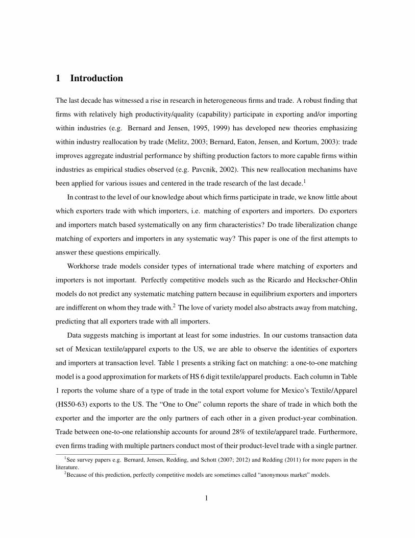
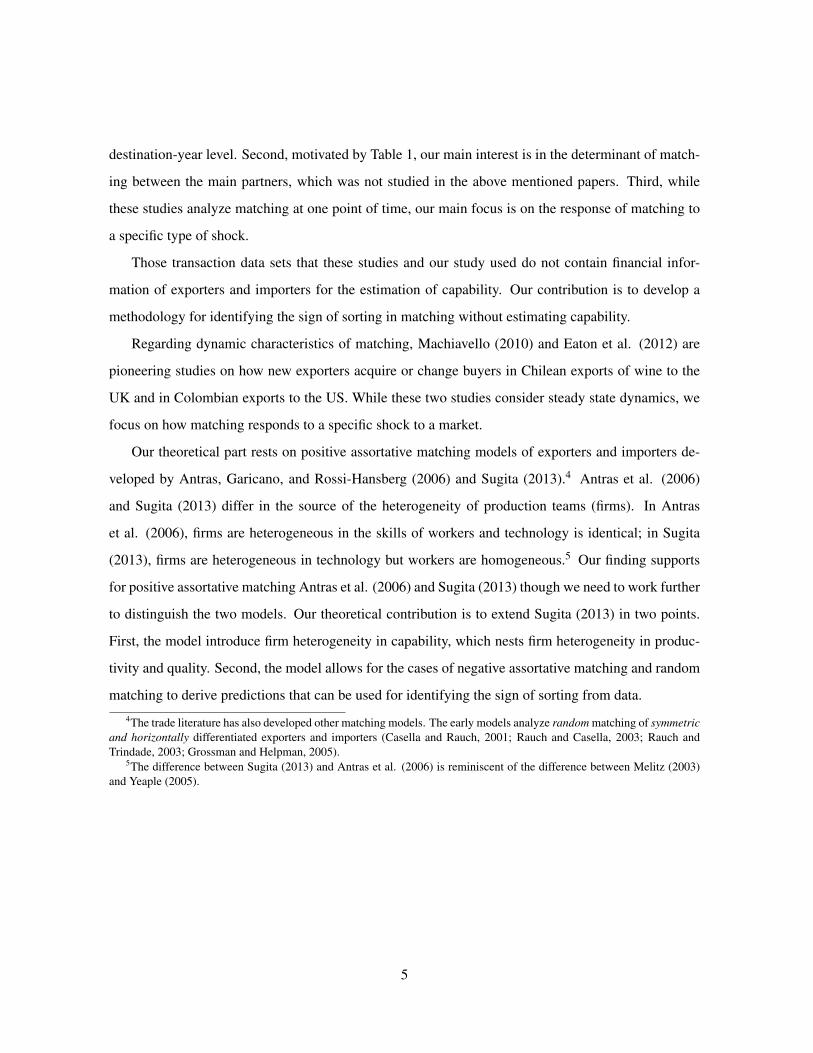
In Case-S, matching function m

x

(x) satisfies the following “matching market clearing” condition.

(Case-S) (M

M

+M

C

) [1� F (x)] = M

U

[G(m

x

(x))�G(y

L

)] for all x � x

L

. (5)

10

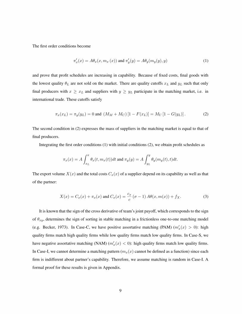
The left hand side of (4) is the mass of suppliers that have higher capability than x and the right hand

side is the mass of final producers who match with them. Figure 2 describes the matching market

clearing condition (5). The left rectangle for suppliers is described in the same way as in Figure 1.

The right rectangle describes the rectangle for US final producers in Figure 1 turned upside down.

Therefore, a lower position in the rectangle expresses a high capability. The right gray area is equal

to the mass of US final producers whose capability is between m

x

(x) and x

L

. The matching market

clearing condition (4) requires the two gray areas to have the same size.

1

0

0

1

F(x)

G(y)

F(x )L

G(y )LExit

F(x)

G(m (x))x

=

MU

Exit

=

MM MC

Suppliers Final Producers

Mexico ChinaThe US

Figure 2: Case-S: Negative Assortative Matching (NAM)

In Case-C and Case-S when systematic matching exist, equilibrium matching depends on the dis-

tributions of final producers and suppliers. As shown in Sugita (2003) for the case of PAM, trade

liberalization causes an additional mechanism of within industry reallocation. In addition to well

known reallocation of production factors among firms, trade liberalization reshuffles matching of firms

in global supply chains as additional mechanism of within industry reallocation.

2.2 Revenue Productivity and Assortative Matching

One of the important differences between workhorse trade models and our matching model is the

divisibility of transaction. On the one hand, workhorse models consider markets where transaction

11

is infinitely divisible and an arbitrage is possible for each unit of good. Sellers are forced to set a

linear price (price per unit of good) that is common for all consumers. Because sellers are indifferent

across buyers, by which markets are sometime called “anonymous”, no systematic matching of buyers

and sellers arises. On the other hand, our matching model considers markets where transaction is

indivisible and arbitrage for each unit of good is not possible. Systematic matching of buyers and

sellers may arise to reflect the complementarity or substitutability of capabilities of buyers and sellers.

Empirical research have developed several empirical measures of firm’s performance under the

assumption of anonymous markets. How do those measures work in a matching market we are con-

sidering? To fully answer this question is clearly beyond the scope of this paper. As one example, this

section chooses one measure, productivity, and analyzes how the sign of sorting (the sign of ✓xy

) and

the coexistence of heterogeneity of importers affect the measurement of productivity of exporters.

We consider “revenue productivity” (or revenue-based total factor productivity), which is estimated

as the residual of a regression of a firm’s revenue, instead of physical outputs, on inputs.10 Revenue

productivity is one of the most widely estimated measures because it is usually difficult for researchers

to obtain information on output prices of each firm. We assume labor is the only production factor for

simplicity. Then, revenue productivity is obtained as real value-added per worker V (x) =

X(x)/PC

x

(x)/w ,

where w is (exogenously given) wage and ˜

P is a price deflator. From X (x) = C

x

(x)+⇡

x

(x), revenue

productivity is written as an increasing function of profits per costs:

V (x) =

w

eP

1 +

⇡

x

(x)

C

x

(x)

�and

⇡

x

(x)

C

x

(x)

=

´x

x

L

✓

x

(t,m

x

(t))dt

c

x

c

(� � 1) ✓(x,m

x

(x)) +

f

x

f

✓

L

. (6)

Our model deviates from standard models of heterogeneous exporters in three points: (1) one-to-

one matching; (2) heterogeneous importers; (3) interactions of capabilities within matches (✓xy

). We

first eliminate the second and the third factors by considering a special case of Case-I, ✓y

= 0, where

there is no essential heterogeneity among final producers. We call this case Case-N (No importer

heterogeneity). In Case-N, all importer receive zero profits and exporter’s profits become ⇡

x

(x) =

A✓(x) � f

x

. Then, profits per costs ⇡x

(x)/C

x

(x) and revenue productivity V (x) behave in the same

way as in standard models of heterogeneous exporters with constant markups and fixed costs such as10See Foster, Haltiwanger, and Syversson (2008) for the differences between revenue productivity and ideal physical

productivity.

12

Melitz (2003) and Baldwin and Harrigan (2008). Second, we introduce importer heterogeneity ✓

y

> 0

in Case-I with ✓

xy

= 0. Revenue productivity turns to behave very differently. The denominator of

⇡

x

(x)/C

x

(x) in (6) increases in m

x

(x) but the numerator does not depend on it. Therefore, V (x)

decreases in partner’s capability m

x

(x). Since matching is random in Case-I, revenue productivity

V (x) is a decreasing function of a random variable of the capability y of partner importers.

Proposition 1. In Case-I (✓xy

= 0) with importer heterogeneity (✓y

> 0), revenue productivity V (x)

of exporters is a decreasing function of a random variable of the capability y of partner importers.

Proposition 1 implies that in Case-I, revenue productivity is a noisy measure of true capability

x even in an environment with no fundamental uncertainty. This would impose a challenge on the

inference of the distribution of true capability x from observed revenue productivity because V (x)

includes partner capability m

x

(x) in a non linear way and the distribution of capability y is typically

unobservable. The gap between the distributions of V (x) and true x would become large when the

capability of final producers is important (✓y

is large) and when the dispersion of y is large.

Finally, we compare revenue productivity V (x) of Case-C and Case-S with that in Case-N. We

consider three models, model-i (i = N,C, S).

Definition 1. Model-i (i = N,C, S) is defined as follows. (1) Each model-i has a ✓ function of

Case-i and an identical set of parameters (except ✓i) and identical distributions of capabilities x and

y; (2) ✓i function and matching function m

i

x

(x) of model i satisfy that ✓N (x, y) = ✓

C

(x,m

C

x

(x)) =

✓

S

(x,m

S

x

(x)) for all x � x

L

.

It is straightforward to show that each model generates an identical cutoff x

L

and an identical

distribution of employment Cx

(x) for active Mexican suppliers. In sum, we compare revenue produc-

tivity under three ✓ functions that generate identical employment. Using these models, we obtain the

following Proposition 2.

Proposition 2. Revenue productivity in model-i (i=N,C, S), V i

(x), satisfy that V S

(x

L

) = V

N

(x

L

) =

V

C

(x

L

) and that V S

(x) > V

N

(x) > V

C

(x) for all x > x

L

.

Proof. d✓

i

(x)/dx = ✓

i

x

(x,m

i

x

(x)) + ✓

i

y

(x,m

i

x

(x))m

i0x

(x) is identical across the three models. Since

✓

C

y

(x,m

C

x

(x))m

C0x

(x) > 0, ✓Ny

(x,m

N

x

(x)) = 0, and ✓

S

y

(x,m

S

x

(x))m

S0x

(x) < 0, we obtain ✓

S

x

(x,m

x

(x)) >

13

✓

N

x

(x,m

x

(x)) > ✓

C

x

(x,m

x

(x)) for all x � x

L

. Since C

x

(x) is identical across the three models and

⇡

i

x

(x

L

) = 0, we obtain the proposition.

The intuition for Proposition 2 is simple. Revenue productivity is increasing in profits per costs. On

one hand, exporter’s costs are increasing in the sales of final goods and depend on the team capability

(✓), which includes partner’s as well as its own capability. On the other hand, exporter’s profits depends

on its contribution within team (✓x

). In Case-S, a high capable supplier matches a low capable final

producer, while in Case-C, a high capable supplier matches a high capable supplier. When producing

the same level of team capability, high capable suppliers in Case-S should make greater contributions

within teams and receive greater profits than those in Case-C.

Proposition 2 implies that the existence of importer heterogeneity affects revenue productivity and

the direction of the effect depends on the sign of sorting. With comkplementarity, the importer het-

erogeneity tends to reduce revenue productivity, while with substitutability, the importer heterogeneity

tends to increase revenue productivity. This may have a potential implication for studies of produc-

tivity involving multiple industries. If industries have different signs of sorting, one should be careful

when comparing revenue productivity across industries.

2.3 Identifying the Sign of Sorting

How can we identify the sign of sorting (the sign of ✓xy

) from typical trade data? One strategy may

be to estimate capabilities x and y for each firm and then to look at their correlation across matches.

However, this strategy faces two difficulties. First, it is difficult to assemble a data set linking detail

financial variables of both exporters and importers to customs transaction data. Second, even with such

detail data, the methodology of estimating capabilities in a matching market is not well established.

A conventional measure of capability developed for a market with infinitely divisible transaction may

not work in a matching market with indivisible transaction.11

11For example, think about using firm’s employment as a proxy for firm’s capability and looking at a correlation ofemployment of exporters and importers across matches. One might want to interpret their positive correlation as evidencefor complementarity-driven PAM and their negative correlation as evidence for substitutability-driven NAM. This strategymight appear reasonable since using employment as a proxy for capability has appeared in previous studies assuming amodel with infinitely divisible transaction. However, looking at employment correlations of exporters and importers is notinformative at all about the sign of sorting in the current matching model. All Case-i (i = I,N, S,C,) including evenCase-S of NAM predict positive correlations simply because importer’s employment is increasing in the amount of importedintermediate goods, which is again increasing in exporter’s employment.

14

We develop an alternative strategy to identify the sign of sorting that uses only customs transaction

data documenting the identities (names or id numbers) of exporters and importers, product categories,

and trade volume. Similar data have recently become available for several countries. The key idea

is that the way firms change their partners in response to a shock to a matching market could differ

across models-i depending on the sign of sorting. Although there will be multiple shocks creating such

changes, we consider a particular shock, an exogenous increase in the mass of Chinese suppliers in the

US market.

2.3.1 Comparative Statics: an Increase in the mass of Chinese Suppliers

Suppose that the mass of Chinese suppliers increases (dMC

> 0). We call this shock “liberalization”

because we will analyze an event of liberalization later that induced a surge in Chinese suppliers in the

US market. For simplicity, we assume positive but negligible switching costs so that a firm changes its

partner only if it strictly prefers the new match to the current match.

We consider how Mexican suppliers and US importers change their partners. Particularly, we focus

on Mexican suppliers that export to the US both before and after liberalization and US final producers

that import from Mexico both before and after liberalization. We call them “continuing Mexican

exporters” and “continuing US importers”, respectively.

In Case-I including Case-N, firms are indifferent about partner’s capability. Therefore, the change

in matching is minimized. Therefore, continuing Mexican exporters and continuing US importers do

not change their partners

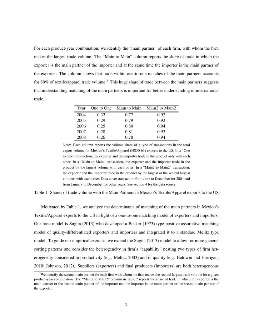
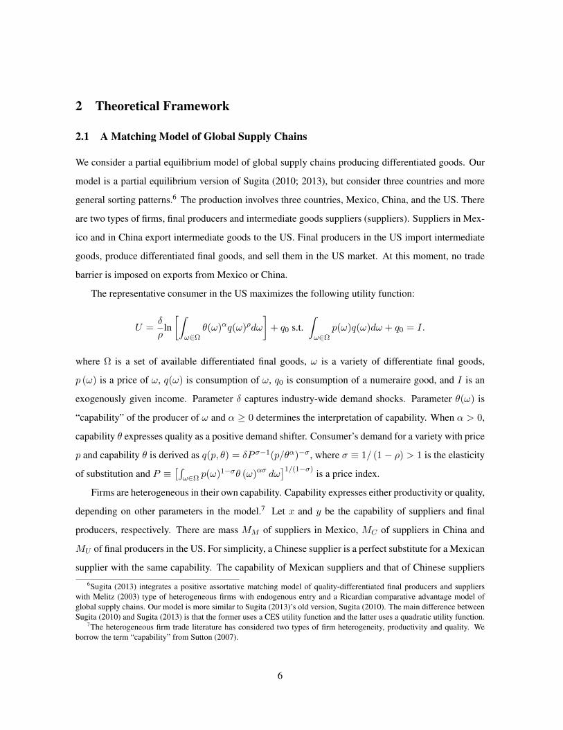
In Case-C, matching function m

x

(x) systematically changes to satisfy the matching market clear-

ing condition (4). Figure 3 describes how Mexican exporters with capability x changes the capability

of their partners from m

0x

(x) to m

1x

(x). After liberalization, the mass of suppliers with higher capa-

bility than x increases by dM

C

[1� F (x)], which is expressed as the left striped area. The mass of US

final producers with higher quality than m

1x

(x) should increase by the size of the right striped area,

the size of which is equal to the size of the left striped area. Therefore, continuing Mexican exporters

downgrade partner’s capability. This means that continuing US importers upgrade partner’s capability.

In Case-S, the change in matching is more complex since the matching market clearing condition

includes the cutoff of final producers y

L

. The change of yL

is in general ambiguous, depending on

15

’

1

00

1

F(x) G(y)

F(x )L

G(y )L

F(x)

G(m (x))x

MUMM MC

Suppliers Final Producers

Mexico China The US

0

dMC

0

0

G(m (x))x1

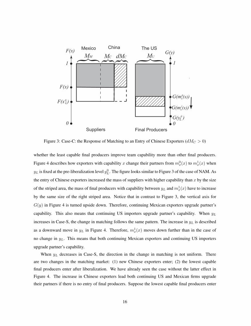
Figure 3: Case-C: the Response of Matching to an Entry of Chinese Exporters (dMC

> 0)

whether the least capable final producers improve team capability more than other final producers.

Figure 4 describes how exporters with capability x change their partners from m

0x

(x) to m

1x

(x) when

y

L

is fixed at the pre-liberalization level y0L

. The figure looks similar to Figure 3 of the case of NAM. As

the entry of Chinese exporters increased the mass of suppliers with higher capability than x by the size

of the striped area, the mass of final producers with capability between y

L

and m

1x

(x) have to increase

by the same size of the right striped area. Notice that in contrast to Figure 3, the vertical axis for

G(y) in Figure 4 is turned upside down. Therefore, continuing Mexican exporters upgrade partner’s

capability. This also means that continuing US importers upgrade partner’s capability. When y

L

increases in Case-S, the change in matching follows the same pattern. The increase in y

L

is described

as a downward move in y

L

in Figure 4. Therefore, m1x

(x) moves down further than in the case of

no change in y

L

. This means that both continuing Mexican exporters and continuing US importers

upgrade partner’s capability.

When y

L

decreases in Case-S, the direction in the change in matching is not uniform. There

are two changes in the matching market: (1) new Chinese exporters enter; (2) the lowest capable

final producers enter after liberalization. We have already seen the case without the latter effect in

Figure 4. The increase in Chinese exporters lead both continuing US and Mexican firms upgrade

their partners if there is no entry of final producers. Suppose the lowest capable final producers enter

16

1

0

0

1

F(x)

G(y)

F(x )L

G(y )=L

F(x)

G(m (x))x

MUMM MC

Suppliers Final Producers

Mexico China The US

0

dMC

G(m (x))x

0

1

G(y )L1

0

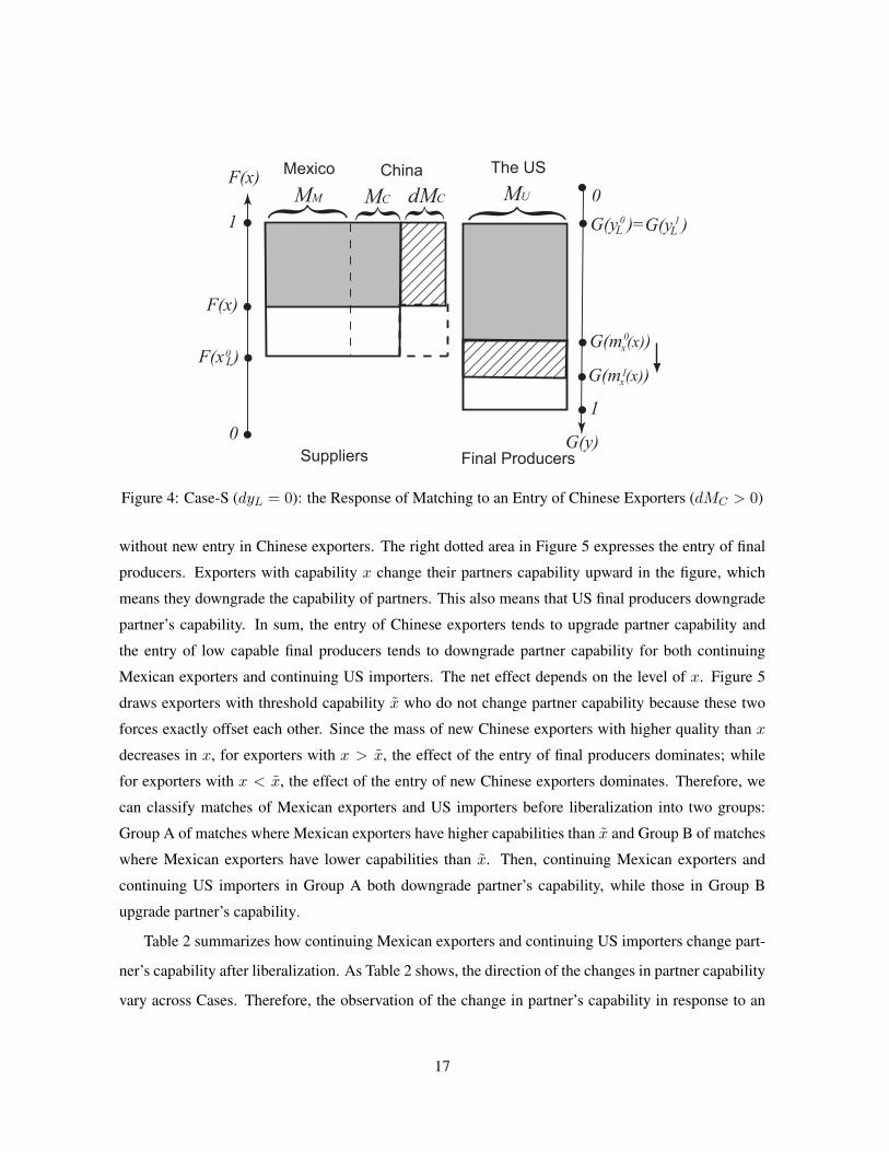
Figure 4: Case-S (dyL

= 0): the Response of Matching to an Entry of Chinese Exporters (dMC

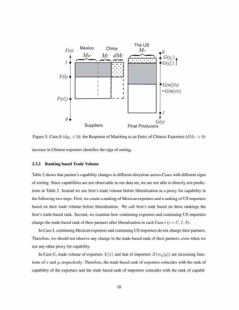
> 0)

without new entry in Chinese exporters. The right dotted area in Figure 5 expresses the entry of final

producers. Exporters with capability x change their partners capability upward in the figure, which

means they downgrade the capability of partners. This also means that US final producers downgrade

partner’s capability. In sum, the entry of Chinese exporters tends to upgrade partner capability and

the entry of low capable final producers tends to downgrade partner capability for both continuing

Mexican exporters and continuing US importers. The net effect depends on the level of x. Figure 5

draws exporters with threshold capability x who do not change partner capability because these two

forces exactly offset each other. Since the mass of new Chinese exporters with higher quality than x

decreases in x, for exporters with x > x, the effect of the entry of final producers dominates; while

for exporters with x < x, the effect of the entry of new Chinese exporters dominates. Therefore, we

can classify matches of Mexican exporters and US importers before liberalization into two groups:

Group A of matches where Mexican exporters have higher capabilities than x and Group B of matches

where Mexican exporters have lower capabilities than x. Then, continuing Mexican exporters and

continuing US importers in Group A both downgrade partner’s capability, while those in Group B

upgrade partner’s capability.

Table 2 summarizes how continuing Mexican exporters and continuing US importers change part-

ner’s capability after liberalization. As Table 2 shows, the direction of the changes in partner capability

vary across Cases. Therefore, the observation of the change in partner’s capability in response to an

17

1

0

0

1

F(x)

G(y)

F(x )L

G(y )L

F(x)G(m (x))x

MUMM MC

Suppliers Final Producers

Mexico ChinaThe US

0

dMC

0

G(m (x))x1

G(y )L1

0

=˜

˜

˜

Figure 5: Case-S (dyL

< 0): the Response of Matching to an Entry of Chinese Exporters (dMC

> 0)

increase in Chinese exporters identifies the sign of sorting.

2.3.2 Ranking based Trade Volume

Table 2 shows that partner’s capability changes in different directions across Cases with different signs

of sorting. Since capabilities are not observable in our data set, we are not able to directly test predic-

tions in Table 2. Instead we use firm’s trade volume before liberalization as a proxy for capability in

the following two steps. First, we create a ranking of Mexican exporters and a ranking of US importers

based on their trade volume before liberalization. We call firm’s rank based on these rankings the

firm’s trade-based rank. Second, we examine how continuing exporters and continuing US importers

change the trade-based rank of their partners after liberalization in each Case-i (i = C, I, S).

In Case-I, continuing Mexican exporters and continuing US importers do not change their partners.

Therefore, we should not observe any change in the trade-based rank of their partners, even when we

use any other proxy for capability.

In Case-C, trade volume of exporters X(x) and that of importers X(m

y

(y)) are increasing func-

tions of x and y, respectively. Therefore, the trade based rank of exporters coincides with the rank of

capability of the exporters and the trade based rank of importers coincides with the rank of capabil-

18

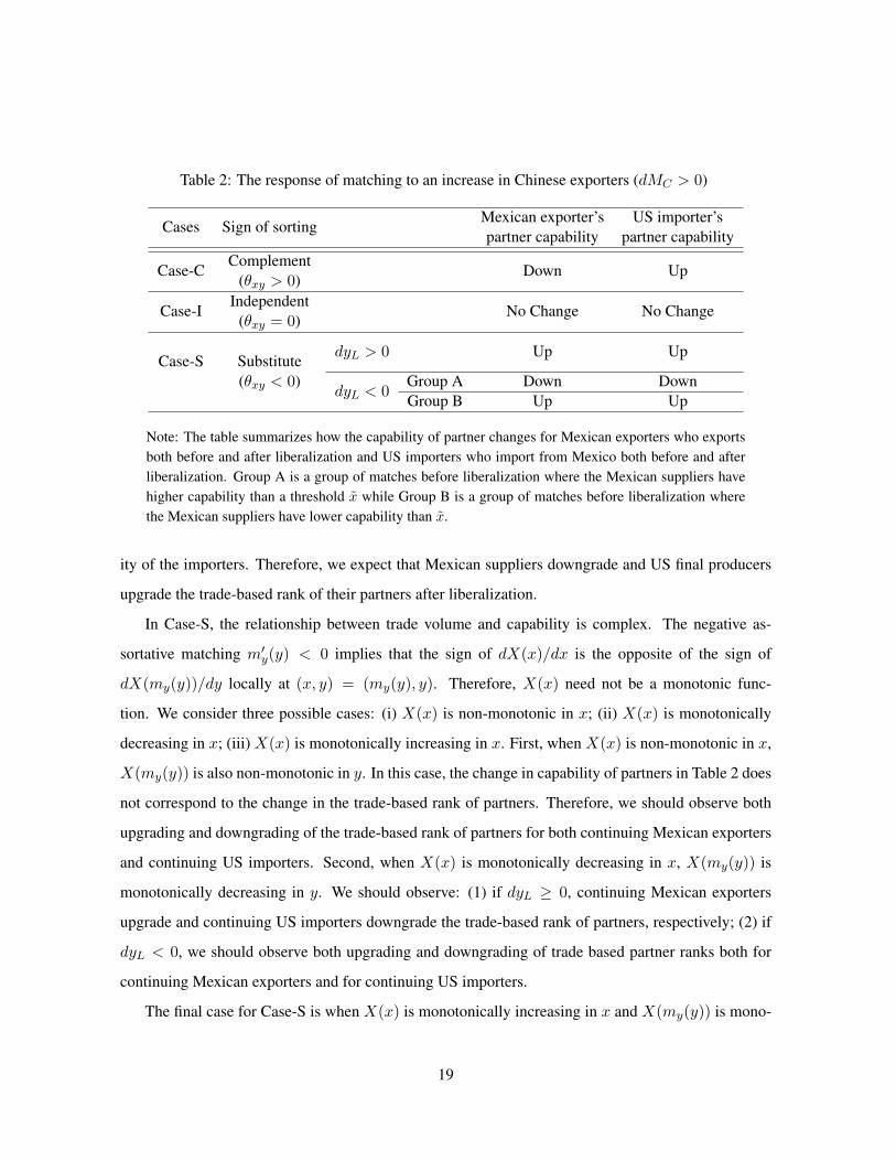
Table 2: The response of matching to an increase in Chinese exporters (dMC

> 0)

Cases Sign of sorting Mexican exporter’s US importer’spartner capability partner capability

Case-C Complement Down Up(✓xy

> 0)

Case-I Independent No Change No Change(✓xy

= 0)

dy

L

> 0 Up UpCase-S Substitute(✓

xy

< 0)dy

L

< 0

Group A Down DownGroup B Up Up

Note: The table summarizes how the capability of partner changes for Mexican exporters who exportsboth before and after liberalization and US importers who import from Mexico both before and afterliberalization. Group A is a group of matches before liberalization where the Mexican suppliers havehigher capability than a threshold x while Group B is a group of matches before liberalization wherethe Mexican suppliers have lower capability than x.

ity of the importers. Therefore, we expect that Mexican suppliers downgrade and US final producers

upgrade the trade-based rank of their partners after liberalization.

In Case-S, the relationship between trade volume and capability is complex. The negative as-

sortative matching m

0y

(y) < 0 implies that the sign of dX(x)/dx is the opposite of the sign of

dX(m

y

(y))/dy locally at (x, y) = (m

y

(y), y). Therefore, X(x) need not be a monotonic func-

tion. We consider three possible cases: (i) X(x) is non-monotonic in x; (ii) X(x) is monotonically

decreasing in x; (iii) X(x) is monotonically increasing in x. First, when X(x) is non-monotonic in x,

X(m

y

(y)) is also non-monotonic in y. In this case, the change in capability of partners in Table 2 does

not correspond to the change in the trade-based rank of partners. Therefore, we should observe both

upgrading and downgrading of the trade-based rank of partners for both continuing Mexican exporters

and continuing US importers. Second, when X(x) is monotonically decreasing in x, X(m

y

(y)) is

monotonically decreasing in y. We should observe: (1) if dyL

� 0, continuing Mexican exporters

upgrade and continuing US importers downgrade the trade-based rank of partners, respectively; (2) if

dy

L

< 0, we should observe both upgrading and downgrading of trade based partner ranks both for

continuing Mexican exporters and for continuing US importers.

The final case for Case-S is when X(x) is monotonically increasing in x and X(m

y

(y)) is mono-

19

tonically decreasing. We reject this case because the model predicts the following unrealistic pattern

on the selection of importers when they face the change in industrial demand, i.e. the change in �.

Lemma 1. Suppose X(x) is monotonically increasing in x in Case-S. A negative shock to the demand

for final goods induce the largest importers to exit.

The reason for Lemma 1 is simple. As in normal cases, a negative demand shock increases y

L

(� #) y

L

") and forces final producer with the lowest capability to exit. If X(x) is increasing in x,

import volume X(m

y

(y)) is decreasing in y. Therefore, final producers who exit due to the negative

demand shock are the largest importers in the industry. It is well established that the probability of

firm’s exit is negatively related to firm size and that facing import competition, smaller firms are more

likely to exit. Lemma 1 contradicts with these established facts on the selection of firms; therefore,

we reject the case that X(x) is monotonically increasing in x. Therefore, for Case-S, we expect two

possibilities: (i) both upgrading and downgrading of the trade-based rank of partners are observed for

both continuing Mexican exporters and US importers; (ii) continuing Mexican exporters upgrade and

continuing US importers downgrade the trade based rank of their main partners.

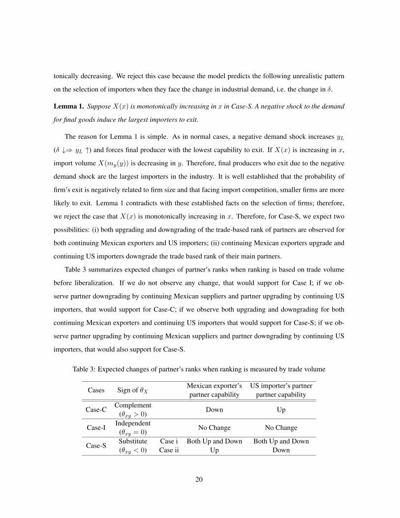
Table 3 summarizes expected changes of partner’s ranks when ranking is based on trade volume

before liberalization. If we do not observe any change, that would support for Case I; if we ob-

serve partner downgrading by continuing Mexican suppliers and partner upgrading by continuing US

importers, that would support for Case-C; if we observe both upgrading and downgrading for both

continuing Mexican exporters and continuing US importers that would support for Case-S; if we ob-

serve partner upgrading by continuing Mexican suppliers and partner downgrading by continuing US

importers, that would also support for Case-S.

Table 3: Expected changes of partner’s ranks when ranking is measured by trade volume

Cases Sign of ✓X

Mexican exporter’s US importer’s partnerpartner capability partner capability

Case-C Complement Down Up(✓xy

> 0)

Case-I Independent No Change No Change(✓xy

= 0)

Case-S Substitute Case i Both Up and Down Both Up and Down(✓

xy

< 0) Case ii Up Down

20

3 The End of the MFA in 2005

As Table 3 summarizes, an exogenous increase in third country exporters at various capability level

(dMC

> 0) can identify the sign of sorting between exporters and importers. This section explains that

the end of the Multi-Fiber Arrangement (MFA) in 2005 brought this type of shock to Mexican exports

of some textile/apparel goods to the US. Specifically, we will exploit three natures of this event. First,

in the US market, the increase in imports from China after the end of the MFA dominated imports from

other countries. Second, the exports by new entrants rather than incumbents accounted for the increase

in Chinese exports after 2005. These new entrants have various levels of capability and some of them

are more productive than incumbents assigned quota licenses before 2005. Third, Mexican exports to

the US significantly dropped among products China faced binding quota in 2004. These features of

the end of the MFA are known from previous studies, so we briefly summarize them here.

The Surge in Chinese Exports to the US The MFA and its successor, the Agreement on Textile

and Clothing, are agreements on quota restriction on textile/apparel imports among the GATT/WTO

member countries. At the GATT Uruguay round, the US (and other member countries) promised to

abolish their quota in four steps: quotas that are equivalent with 16, 17, 18, and 49% of imports in

1990 were removed on January 1, 1995, 1998, 2002, and 2005, respectively.

The quota removal of 2005 triggered a surge in imports to the US, mostly from China. Bram-

billa, Khandelwal, and Schott (2009) estimated that in 2005, US imports from China disproportionally

increased by 271%, while imports from almost all other countries decreased. Seeing a huge import

growth, the US and China had agreed to impose new quota until 2008, but imports from China never

went back to the pre-2005 level. The new quota system covered fewer product categories than the old

system (Dayaranta-Banda and Whalley, 2007 ) and the level of quota is substantially greater than the

MFA level (see Table 2 in Brambilla et al., 2009).

Exports by New and More Productive Entrants Khandelwal, Schott, and Wei (2013) investigated

Chinese customs transaction data and decomposed the increase in Chinese exports after the quota

removal into intensive and extensive margins. The authors found that the increase in Chinese exports

of quota constrained products were mostly driven by the entry of Chinese firms who did not export the

21

product before 2005. Furthermore, while incumbent exporters include a number of state owned firms,

these new exporters include more private and foreign firms, which are more productive than state

owned firms. Indeed, the distribution of unit prices of new entrants has a lower mean and a greater

support than that of unit prices of incumbent exporters. These findings suggest that the removal of

import quota induced new entrants at various levels of capability, which corresponds dMC

> 0 in the

previous section.12

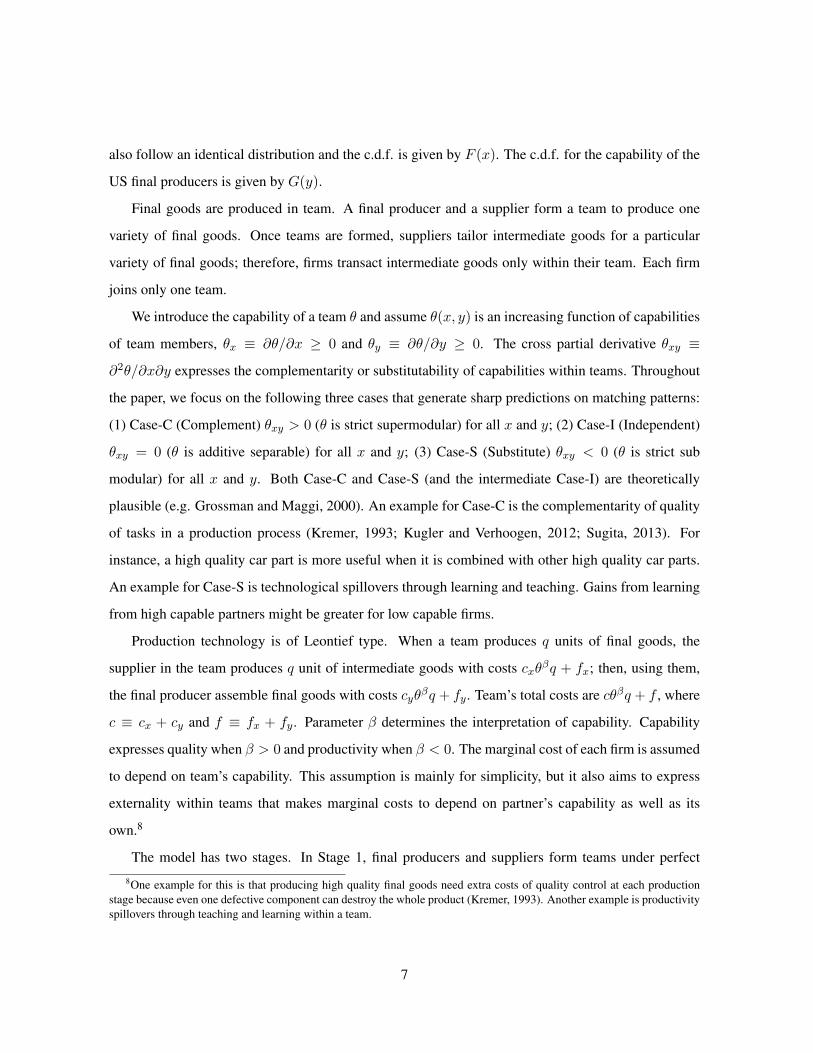
Mexican Exports and Competition from China Mexico had already had tariff-and-quota free ac-

cess to the US market through the North American free trade agreement before 2005.13 At the end of

MFA, Mexico had lost its advantage to third country exporters and faced an increase in competition

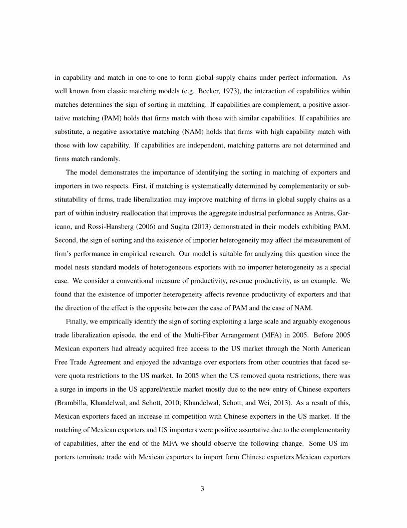
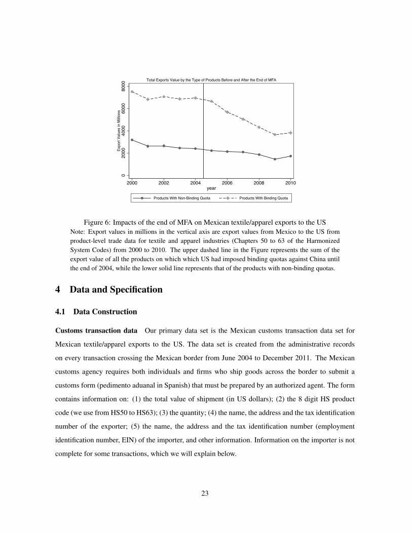
with Chinese exporters in the US market. Figure 6 is based on the data on Mexican product-level ex-

ports to the US for textile and apparel industries (Chapters 50 to 63 of the Harmonized System Codes)

from 2000 to 2010. The upper dashed line in Figure 6 represents the sum of the export value of all the

products on which the US had imposed binding quotas against China until the end of 2004, while the

lower solid line represents that of the products with non-binding quotas. The vertical line in year 2005

represents the year in which the MFA expired, implying that any of the products that were included in

the MFA had no longer quotas. The figure shows that the two series had moved in parallel before the

expiration of the MFA, while the total value of the exports of the products with the US binding quotas

against China exhibits a much larger decline after the expiration, suggesting that the surge of Chinese

exports to the U.S. due to the end of MFA had a substantial impact on the competition that Mexican

exporters face in the U.S. market and on the availability of foreign sellers for the U.S. importers.12These findings contradicts with the predictions of models of optimal quota allocations. If quota licenses are efficiently

allocated to the most capable firms, then the removal of quota mainly increases exports by incumbents and the new exportersare the least capable firms. See Khandelwal, Schott, and Wei (2013) for a formal demonstration of this claim. Seeing theopposite patten in data, Khandelwal, Schott, and Wei (2013) therefore concluded the allocation of quota licenses were fardifferent from the optimal allocation and produced additional inefficiency.

13In NAFTA, the US market was liberalized to Mexican exports in 1994, 1999, and 2003.

22

020

0040

0060

0080

00Ex

port

Valu

es in

Milli

ons

2000 2002 2004 2006 2008 2010year

Products With Non-Binding Quota Products With Binding Quota

Total Exports Value by the Type of Products Before and After the End of MFA

Figure 6: Impacts of the end of MFA on Mexican textile/apparel exports to the USNote: Export values in millions in the vertical axis are export values from Mexico to the US fromproduct-level trade data for textile and apparel industries (Chapters 50 to 63 of the HarmonizedSystem Codes) from 2000 to 2010. The upper dashed line in the Figure represents the sum of theexport value of all the products on which which US had imposed binding quotas against China untilthe end of 2004, while the lower solid line represents that of the products with non-binding quotas.

4 Data and Specification

4.1 Data Construction

Customs transaction data Our primary data set is the Mexican customs transaction data set for

Mexican textile/apparel exports to the US. The data set is created from the administrative records

on every transaction crossing the Mexican border from June 2004 to December 2011. The Mexican

customs agency requires both individuals and firms who ship goods across the border to submit a

customs form (pedimento aduanal in Spanish) that must be prepared by an authorized agent. The form

contains information on: (1) the total value of shipment (in US dollars); (2) the 8 digit HS product

code (we use from HS50 to HS63); (3) the quantity; (4) the name, the address and the tax identification

number of the exporter; (5) the name, the address and the tax identification number (employment

identification number, EIN) of the importer, and other information. Information on the importer is not

complete for some transactions, which we will explain below.

23

Assign firm IDs We assigned identification numbers for both Mexican exporters and US importers

(exporter-ID and importer-ID) throughout the data set. It is straightforward to assign exporter-ids for

Mexican exporters since the Mexican tax number uniquely identifies each Mexican firm. However,

there exists a challenge for assigning importer-ids for US firms. It is known that one US firm often has

multiple names, addresses, and EINs. This happens because a firm sometimes uses multiple names or

changes names, owns multiple plants, and changes tax numbers. Therefore, simply matching firms by

one of three linking variables (names, addresses and EINs) would wrongly assign more than one id for

one US buyer and would result in overestimating the number of US buyers for each Mexican exporter.

We used a series of methods developed in the record linkage research for data cleaning to assign

importer-ID.14 First, since the focus of our study is firm-to-firm matching, we dropped transactions for

which exporters were individuals and courier companies (e.g. FedEx, UPS, etc.). Second, a company

name often included generic words that did not help identify a particular company such as legal terms

(e.g. “Co.”) and words commonly appearing in the industry (e.g. “apparel”). We removed these

words from company names. Third, we standardized addresses by a software, ZP4, which received a

CASS certification of address cleaning by the United States Postal Services. Fourth, we prepared lists

of fictitious names, previous names and name abbreviations, a list of addresses of company branches,

and a list of EINs from data on company information, Orbis made by Bureau van Dijk, which covered

20 millions company branches, subsidiaries, and headquarters in the US. We used Orbis information

for manufacturing firms and intermediary firms (wholesales and retails) due to the capacity of our

workstation. For each HS 2 digit industry, we matched names within customs data and names between

customs data and name lists from Orbis mentioned above; we did similar matches for address and

EIN. When matching them, we used fuzzy matching techniques allowing small typographical errors.15

Fifth, using matched relations and a software of the network theory, we created clusters of information

(names, addresses, EINs) in which one cluster identifies one firm. We identified a cluster basically

under a rule that each entry in a cluster fuzzy matches with some other entries in the cluster through

two of three linking variables (names, addresses, EINs). Finally, we assigned importer-ids for clusters.14An excellent textbook for record linkage is Herzog, Scheuren, and Winkler (2007). A webspage of “Virtual

RDC@Cornell” (http://www2.vrdc.cornell.edu/news/) at Cornell University is also a great source of information on datacleaning. We particularly benefit from lecture slides on “Record Linkage” by John Abowd and Lars Vilhuber. We plan toprepare a long Appendix on data cleaning in the next version of this paper.

15We used Jaro-Winkler metric in the Record Linkage package of R and other methods, which will be explained in thenext version.

24

Dropping missing information From the above processes, the data set includes information on ex-

porter ids, importer ids, value of shipment, product code, and transaction date. We then aggregated

value of shipment for a given combination of exporter, importer, HS 6 digit product, and year.16 In-

formation on importers was not complete for some transactions. Mexican customs do not mandate

the custom agents to report information of US importers for processing re-exports called Maquiladora

(now called IMMEX since 2007) exports which are exports by the outsourcing contracts between

Mexican firms and the foreign (in most cases US) firms. The exemption of the information is because

Maquiladora/IMMEX exporters register the information of buyers in advance.

The Mexican customs transaction data set covers only information from June to December for

2004. To make the information of other years comparable to that of 2004, we dropped observations

from January to May for other years, too. We remark that the “Main to Main” shares in Table 1 changed

very little (a 1 percentage point change only for 2007) from the drop of January-May observations.

Therefore, we believe this drop of observations caused little selection problems.

For each exporter-product (HS6)-year combination, we dropped entries for which we could not

identify importers for more than 20 percent of export values. Though we dropped around 30-40 per-

cent of exporters and around 60-70 percent of export values, we think sample selection problems are

likely to be small. Non-Maquiladora trade and Maquiladora trade show very similar patterns on firm’s

average number of partners and Main-to-Main trade shares (as in Table 1). Further notes of the data

construction and the section issue will be available in the next version of this paper.

Ranking The next step is to create rankings of exporters and importers based on their trade volume.

In the model, all matches are one-to-one, but in data, exporters and importers may have multiple

partners. We created rankings of firms by trade volume with their main partners in 2004. Let xempt

be exports of product p from exporter e to importer m in year t, Mpt

(e) be the set of importers with

which exporter e trade p in year t and E

pt

(m) be the set of exporters with which importer m trade p

in year t. Exporter e’s export to the main partner was obtained as EX

ept

= max

m2Mpt

(e) xempt

and

importer m’s import from the main partner was obtained as IMmpt

= max

e2Ept

(m) xempt

. Finally, we

created the trade-based ranking of exporters by EX

ep2004 and the trade-based ranking of importers by16We decided to aggregate the data from the Mexican 8-digit to 6-digit because the Mexican 6-digit code is same as the

HS code while it is difficult to construct a concordance between the Mexican 8-digit and the U.S. 10-digit, at which the MFAquotas are defined.

25

IM

mp2004. 17

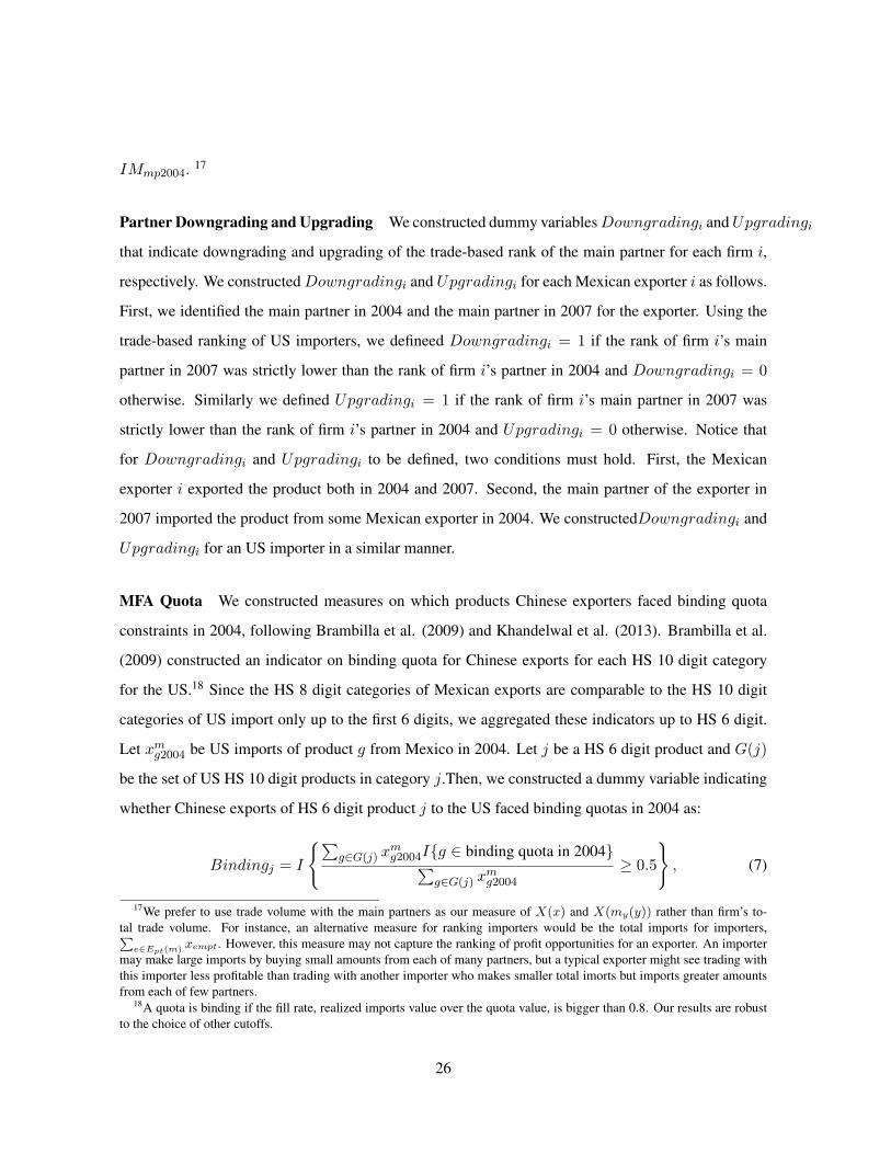
Partner Downgrading and Upgrading We constructed dummy variables Downgrading

i

and Upgrading

i

that indicate downgrading and upgrading of the trade-based rank of the main partner for each firm i,

respectively. We constructed Downgrading

i

and Upgrading

i

for each Mexican exporter i as follows.

First, we identified the main partner in 2004 and the main partner in 2007 for the exporter. Using the

trade-based ranking of US importers, we defineed Downgrading

i

= 1 if the rank of firm i’s main

partner in 2007 was strictly lower than the rank of firm i’s partner in 2004 and Downgrading

i

= 0

otherwise. Similarly we defined Upgrading

i

= 1 if the rank of firm i’s main partner in 2007 was

strictly lower than the rank of firm i’s partner in 2004 and Upgrading

i

= 0 otherwise. Notice that

for Downgrading

i

and Upgrading

i

to be defined, two conditions must hold. First, the Mexican

exporter i exported the product both in 2004 and 2007. Second, the main partner of the exporter in

2007 imported the product from some Mexican exporter in 2004. We constructedDowngrading

i

and

Upgrading

i

for an US importer in a similar manner.

MFA Quota We constructed measures on which products Chinese exporters faced binding quota

constraints in 2004, following Brambilla et al. (2009) and Khandelwal et al. (2013). Brambilla et al.

(2009) constructed an indicator on binding quota for Chinese exports for each HS 10 digit category

for the US.18 Since the HS 8 digit categories of Mexican exports are comparable to the HS 10 digit

categories of US import only up to the first 6 digits, we aggregated these indicators up to HS 6 digit.

Let xmg2004 be US imports of product g from Mexico in 2004. Let j be a HS 6 digit product and G(j)

be the set of US HS 10 digit products in category j.Then, we constructed a dummy variable indicating

whether Chinese exports of HS 6 digit product j to the US faced binding quotas in 2004 as:

Binding

j

= I

(Pg2G(j) x

m

g2004I{g 2 binding quota in 2004}P

g2G(j) xm

g2004

� 0.5

), (7)

17We prefer to use trade volume with the main partners as our measure of X(x) and X(my

(y)) rather than firm’s to-tal trade volume. For instance, an alternative measure for ranking importers would be the total imports for importers,P

e2Ept(m) xempt

. However, this measure may not capture the ranking of profit opportunities for an exporter. An importermay make large imports by buying small amounts from each of many partners, but a typical exporter might see trading withthis importer less profitable than trading with another importer who makes smaller total imorts but imports greater amountsfrom each of few partners.

18A quota is binding if the fill rate, realized imports value over the quota value, is bigger than 0.8. Our results are robustto the choice of other cutoffs.

26

where the indicator function I{X} = 1 if X is true and I{X} = 0 otherwise. We chose the cutoff

value as 0.5 but the choice of this value is not likely to affect the results since most of values inside the

indicator function are close to either one or zero.

4.2 Specification

4.2.1 Mexican exporter’s change of US partners

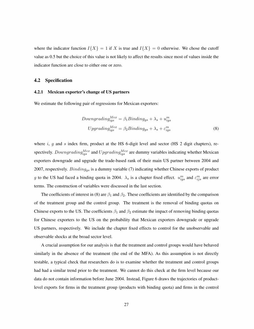
We estimate the following pair of regressions for Mexican exporters:

Downgrading

Mex

igs

= �1Binding

gs

+ �

s

+ u

m

igs

Upgrading

Mex

igs

= �2Binding

gs

+ �

s

+ "

m

igs

(8)

where i, g and s index firm, product at the HS 6-digit level and sector (HS 2 digit chapters), re-

spectively. Downgrading

Mex

igs

and Upgrading

Mex

igs

are dummy variables indicating whether Mexican

exporters downgrade and upgrade the trade-based rank of their main US partner between 2004 and

2007, respectively. Binding

gs

is a dummy variable (7) indicating whether Chinese exports of product

g to the US had faced a binding quota in 2004. �

s

is a chapter fixed effect. u

m

igs

and "

m

ijs

are error

terms. The construction of variables were discussed in the last section.

The coefficients of interest in (8) are �1 and �2. These coefficients are identified by the comparison

of the treatment group and the control group. The treatment is the removal of binding quotas on

Chinese exports to the US. The coefficients �1 and �2 estimate the impact of removing binding quotas

for Chinese exporters to the US on the probability that Mexican exporters downgrade or upgrade

US partners, respectively. We include the chapter fixed effects to control for the unobservable and

observable shocks at the broad sector level.

A crucial assumption for our analysis is that the treatment and control groups would have behaved

similarly in the absence of the treatment (the end of the MFA). As this assumption is not directly

testable, a typical check that researchers do is to examine whether the treatment and control groups

had had a similar trend prior to the treatment. We cannot do this check at the firm level because our

data do not contain information before June 2004. Instead, Figure 6 draws the trajectories of product-

level exports for firms in the treatment group (products with binding quota) and firms in the control

27

group (products with non-binding quota). The figure shows no differential trend in exports of the two

groups several years before the end of the MFA (the treatment).

Positive values of �1 and �2 mean that Mexican exporters downgrade or upgrade more frequently

in industries (products) that faced an increase in competition with Chinese exporters than in other

industries. Table 4 summarizes expected combinations of �1 and �2 for each sign of sorting in

matching: (1) �1 > 0 and �2 = 0 for complementarity-driven positive assortative matching (Case-

C); (2) �1 = 0 and �2 = 0 for capability-independent random matching (Case-I); (3)�1 > 0 and

�2 > 0 for substitutability-driven negative assortative matching (Case-S); (4) �1 = 0 and �2 > 0 for

substitutability-driven negative assortative matching (Case-S).

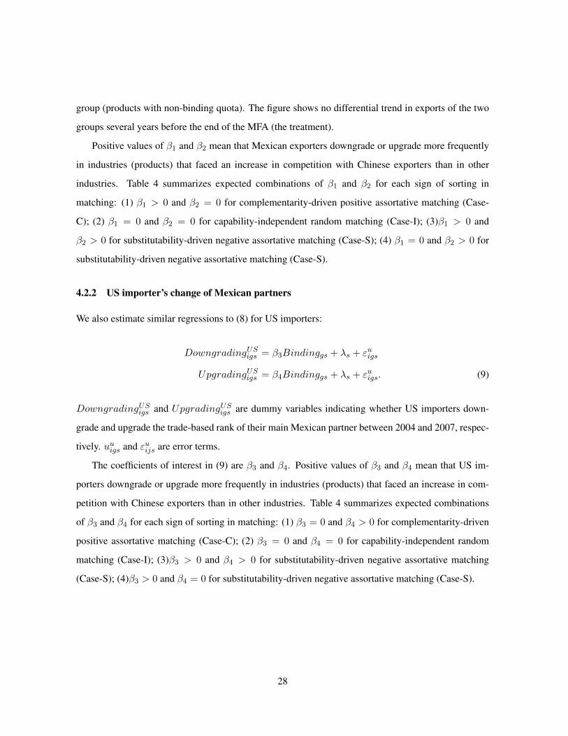
4.2.2 US importer’s change of Mexican partners

We also estimate similar regressions to (8) for US importers:

Downgrading

US

igs

= �3Binding

gs

+ �

s

+ "

u

igs

Upgrading

US

igs

= �4Binding

gs

+ �

s

+ "

u

igs

. (9)

Downgrading

US

igs

and Upgrading

US

igs

are dummy variables indicating whether US importers down-

grade and upgrade the trade-based rank of their main Mexican partner between 2004 and 2007, respec-

tively. uuigs

and "

u

ijs

are error terms.

The coefficients of interest in (9) are �3 and �4. Positive values of �3 and �4 mean that US im-

porters downgrade or upgrade more frequently in industries (products) that faced an increase in com-

petition with Chinese exporters than in other industries. Table 4 summarizes expected combinations

of �3 and �4 for each sign of sorting in matching: (1) �3 = 0 and �4 > 0 for complementarity-driven

positive assortative matching (Case-C); (2) �3 = 0 and �4 = 0 for capability-independent random

matching (Case-I); (3)�3 > 0 and �4 > 0 for substitutability-driven negative assortative matching

(Case-S); (4)�3 > 0 and �4 = 0 for substitutability-driven negative assortative matching (Case-S).

28

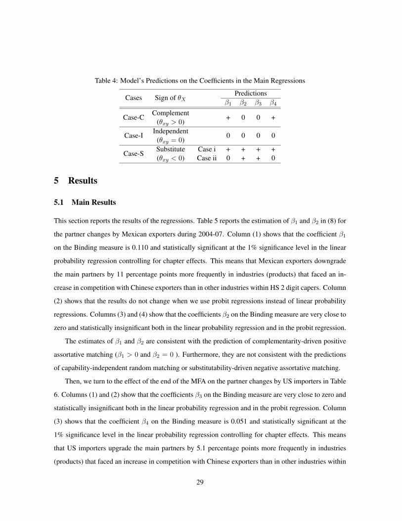
Table 4: Model’s Predictions on the Coefficients in the Main Regressions

Cases Sign of ✓X

Predictions�1 �2 �3 �4

Case-C Complement + 0 0 +(✓xy

> 0)

Case-I Independent 0 0 0 0(✓xy

= 0)

Case-S Substitute Case i + + + +(✓

xy

< 0) Case ii 0 + + 0

5 Results

5.1 Main Results

This section reports the results of the regressions. Table 5 reports the estimation of �1 and �2 in (8) for

the partner changes by Mexican exporters during 2004-07. Column (1) shows that the coefficient �1

on the Binding measure is 0.110 and statistically significant at the 1% significance level in the linear

probability regression controlling for chapter effects. This means that Mexican exporters downgrade

the main partners by 11 percentage points more frequently in industries (products) that faced an in-

crease in competition with Chinese exporters than in other industries within HS 2 digit capers. Column

(2) shows that the results do not change when we use probit regressions instead of linear probability

regressions. Columns (3) and (4) show that the coefficients �2 on the Binding measure are very close to

zero and statistically insignificant both in the linear probability regression and in the probit regression.

The estimates of �1 and �2 are consistent with the prediction of complementarity-driven positive

assortative matching (�1 > 0 and �2 = 0 ). Furthermore, they are not consistent with the predictions

of capability-independent random matching or substitutability-driven negative assortative matching.

Then, we turn to the effect of the end of the MFA on the partner changes by US importers in Table

6. Columns (1) and (2) show that the coefficients �3 on the Binding measure are very close to zero and

statistically insignificant both in the linear probability regression and in the probit regression. Column

(3) shows that the coefficient �4 on the Binding measure is 0.051 and statistically significant at the

1% significance level in the linear probability regression controlling for chapter effects. This means

that US importers upgrade the main partners by 5.1 percentage points more frequently in industries

(products) that faced an increase in competition with Chinese exporters than in other industries within

29

HS 2 digit capers. Column (4) shows that the results do not change when we use probit regressions

instead of linear probability regressions.

The positive estimate of �4 implies that US importers improve their matching from liberalization

of imports from China even when they do not directly use products made in China. This finding is

similar to Amiti and Konings (2007) who found liberalization of tariffs on intermediate goods improve

the productivity of even firms not using imported intermediate goods for Indonesian firms. These

findings are surprising in views of standard models of heterogeneous importers where only firms that

use imported intermediate goods can benefit from liberalization of intermediate goods (Kasahara and

Lapham, 2013; Halpern, Koren, and Szeidl, 2011). As a theoretical explanation for the Amiti-Konings

finding, Sugita (2013) demonstrated that final producers improve matching with domestic intermediate

goods suppliers in face to liberalization of intermediate goods in a positive assortative matching model.

Our finding supports for Sugita(2013)’s prediction.

Again, the estimates of �3 and �3 are consistent with the prediction of complementarity-driven

positive assortative matching (�3 = 0 and �4 > 0 ). Furthermore, they are not consistent with the

predictions of capability-independent random matching or substitutability-driven negative assortative

matching.

In sum, for both Mexican exporter and US importer regressions, we find evidence of complementarity-

based positive assortative matching, ruling out the possibility of random matching and negative assor-

tative matching.

5.2 Robustness Check

5.2.1 Upgrading and Downgrading Analysis at the Same Time

So far we have analyzed downgrading and upgrading separately, one at a time. In the earlier analysis

we have put together upgrading and staying in the same category as opposed to downgrading when

we analyze downgrading, and downgrading and staying in the same category as opposed to upgrading

when we analyze upgrading. We run ordered probit regressions, in which we use the dependent variable

indicating downgrading if the value is -1, staying if the value is zero and upgrading if the value is 1,

to take into account the fact that these two categories are different. Table 7 shows the results. The

coefficients in these regressions do not have quantitative information themselves, and their signs do not

30

contain even qualitative information on the probability of staying but do convey qualitative information

on the relative probability of downgrading and upgrading. The results that the coefficient from Mexican

exporters regression is negative and significant while that from the US importer regression is positive

and significant suggest that Mexican exporters of the affected products are more likely to downgrade

rather than upgrade their US buyers than those of the non-affected products and that US importers of

the affected products are more likely to upgrade rather than downgrade their Mexican sellers than those

of the non-affected products.

5.2.2 Different Time Periods

In table , we present the results of the effect of the end of the MFA on downgrading of US partners for

Mexican exporters for the period (1) between 2004 and 2006 (2) between 2004 and 2007, which were

already reported, and (3) between 2004 and 2008. Column (1) shows that the coefficient is still positive

0.050 but statistical significant only at the 10% significance level in the linear probability regression.

Column (2) shows that the effect becomes bigger in 2007 than in 2006, suggesting that the changes

of partners take place gradually. Column (3) shows that the coefficient is a little smaller for the case

of using 2008 as the final period than that of 2007. One reason for this may be that the trade crisis,

which started in the second half of 2008, produces the demand shock hitting both types of exporters.

Another reason may be that the composition of exporters and importers remaining in the sample differ

between 2007 and 2008. Column (4), (5) and (6) show that the results do not change when we use

probit regressions instead of linear probability regressions.

In table we present the corresponding results for US importers. Column (1) shows that the coef-

ficient on the Binding measure is 0.033 and statistically significant at the 5% significance level in the

linear probability regression for the case of 2006 as the final period. This coefficient now increases

for the case of 2007, which is shown in Column (2). Column (3) shows that the coefficient is further

a little bigger for the case of using 2008 as the final pored than that of 2007. Again, this may also

be because of the difference in the composition of exporters and importers remaining in the sample

in 2007 and 2008. Column (4), (5) and (6) show that the results do not change when we use probit

regressions instead of linear probability regressions. The results are again consistent with the gradual

adjustment.

31

The results of this section suggest that our qualitative conclusion is robust to the choice of the final

period and that the adjustment of the partner upgrading and downgrading happens gradually.

6 Conclusion

This paper has examined the determinants of exporters-importers matches using customs transaction

data from Mexican textile/apparel exports to the US. We found evidence of one-to-one positive as-

sortative matching driven by complementarity of productivity/quality within matches in Antras et al.

(2006) and Sugita (2010). First, both exporters and importers concentrate more than 80% of product-

level trade volume on transaction with a single partner firm. Second, increases in Chinese exporters to

the US market due to the end of the multi-fiber arrangement caused Mexican exporters to downgrade

but allowed US importer to upgrade the trade-based rank of their main partners.

Our finding suggests trade liberalization improves matching of firms in global supply chains as a

part of within industry reallocation that improves the aggregate industrial productivity. Quantification

of this new gains using more detail data on exporters and importers is left for future research.

References

[1] Amiti, Mary, and Jozef Konings. 2007. “Trade Liberalization, Intermediate Inputs, and Produc-

tivity: Evidence from Indonesia.” American Economic Review, 97(5): 1611–38.

[2] Antràs, Pol, Luis Garicano, and Esteban Rossi-Hansberg. 2006. “Offshoring in a Knowledge

Economy.” Quarterly Journal of Economics, 121(1): 31–77.

[3] Baldwin, Richard, and James Harrigan. 2011. “Zeros, Quality and Space: Trade Theory and

Trade Evidence.” American Economic Journal: Microeconomics, 3(May): 1–3.

[4] Becker, Gary S. 1973. “A Theory of Marriage: Part I.” Journal of Political Economy, 81(4):

813–46.

[5] Bernard, Andrew B., and J. Bradford Jensen. 1995. “Exporters, Jobs, and Wages in U.S. Manu-

facturing: 1976-1987.” Brookings Papers on Economic Activity. Microeconomics,1995: 67-119

32

[6] Bernard, Andrew B., and J. Bradford Jensen. 1999. “Exceptional Exporter Performance: Cause,

Effect, or Both?” Journal of International Economics, 47(1): 1–25.

[7] Bernard, Andrew B., J. Bradford Jensen, Stephen J. Redding, and Peter K. Schott. 2007. “Firms

in International Trade.” Journal of Economic Perspectives, 21(3): 105–30.

[8] Bernard, Andrew B., J. Bradford Jensen, Stephen J. Redding, and Peter K. Schott. 2012. “The

Empirics of Firm Heterogeneity and International Trade,” Annual Review of Economics, 4, 283-

313

[9] Bernard, Andrew B., Andreas Moxnes, and Karen Helene Ulltveit-Moe. 2013. “Two-Sided Het-

erogeneity and Trade.” CEPR Discussion Paper 9681.

[10] Blum, Bernardo S., Sebastian Claro, and Ignatius Horstmann. 2010. “Facts and Figures on Inter-

mediated Trade.” American Economic Review Paper and Proceedings, 100(2): 419-23.

[11] Blum, Bernardo S., Sebastian Claro, and Ignatius Horstmann. 2011. “In-

termediation and the Nature of Trade Costs: Theory and Evidence.”

http://www.rotman.utoronto.ca/bblum/personal/front.htm.

[12] Brambilla, Irene, Amit K. Khandelwal, and Peter K. Schott. 2010. “China’s Experience under the

Multi-fiber Arrangement (MFA) and the Agreement on Textiles and Clothing (ATC).” Robert C.

Feenstra and Shang-Jin Wei ed., China’s Growing Role in World Trade. University of Chicago

Press: 345-387.

[13] Carballo, Jerónimo, Gianmarco Ottaviano, Christian Volpe Martincus. 2013. “The Buyer Margins

of Firms’ Exports.” CEPR Discussion Paper 9584.

[14] Casella, Alessandra, and James E. Rauch. 2002 “Anonymous market and group ties in interna-

tional trade.” Journal of International Economics, 58(1): 19-47.

[15] Dayarantna-Banda, OG and John Whalley. 2007. “After the MFA, the CCAs (China Containment

Agreements).” CIGI working paper No. 24.

[16] Drozd, Lukasz A., and Jaromir B. Nosal. 2012. “Understanding international prices: Customers

as capital.” American Economic Review, 102(1): 364-395.

33

[17] Eaton, Jonathan, Marcela Eslava, David Jinkins, C. J. Krizan, and James Tybout. 2012 “A Search

and Learning Model of Export Dynamics.” mimeo.

[18] Eaton, Jonathan, Samuel Kortum, and Francis Kramarz. 2011. “An Anatomy of International

Trade: Evidence from French Firms.” Econometrica, 79(5): 1453-1498.

[19] Foster, Lucia, John Haltiwanger, and Chad Syverson. 2008. “Reallocation, Firm Turnover, and

Efficiency: Selection on Productivity or Profitability?” American Economic Review, 98(1): 394–

425.

[20] Grossman, Gene M., and Elhanan Helpman. 2005. “Outsourcing in a Global Economy.” Review

of Economic Studies, 72(1): 135-59.

[21] Halpern, László, Miklós Koren, and Adam Szeidl. 2011. “Imported Inputs and Productivity.”

http://miklos.koren.hu/view/list/.

[22] Herzog, Thomas N., Fritz J. Scheuren, and William E. Winkler. Data quality and record linkage

techniques. Springer, 2007.

[23] Johnson, Robert C. 2012. “Trade and Prices with Heterogeneous Firms.” Journal of International

Economics, 86 (1): 43-56.

[24] Khandelwal, Amit K., Peter K. Schott, and Shang-Jin Wei. 2013. “Trade Liberalization and Em-

bedded Institutional Reform: Evidence from Chinese Exporters.” American Economics Review,

103(6): 2169-95

[25] Kasahara, Hiroyuki, and Beverly Lapham. 2013. “Productivity and the Decision to Import and

Export: Theory and Evidence.” Journal of International Economics, 89(2): 297-316.

[26] Kremer, Michael. 1993. “The O-Ring Theory of Economic Development.” Quarterly Journal of

Economics, 108(3): 551–75.

[27] Kugler, Maurice, and Eric Verhoogen. 2012. “Prices, Plant Size, and Product Quality.” Review

of Economic Studies, 79(1): 307-339

34

[28] Macchiavello, Rocco. 2010. “Development Uncorked: Reputation Ac-

quisition in the New Market for Chilean Wines in the UK.”

http://www2.warwick.ac.uk/fac/soc/economics/staff/academic/macchiavello/

[29] Melitz, Marc J. 2003. “The Impact of Trade on Intra-Industry Reallocations and Aggregate In-

dustry Productivity.” Econometrica, 71(6): 1695–725.

[30] Pavcnik, Nina. 2002. “Trade Liberalization, Exit, and Productivity Improvements: Evidence from

Chilean Plants.” Review of Economic Studies, 69(1): 245-76.

[31] Rauch, James E., and Alessandra Casella. 2003. “Overcoming Informational Barriers to Interna-

tional Resource Allocation: Prices and Ties.” Economic Journal, 113(484): 21-42.

[32] Rauch, James E., and Vitor Trindade. 2003. “Information, International Substitutability, and

Globalization.” American Economic Review, 93(3): 775-91.

[33] Redding, Stephen J. 2011. “Theories of Hetrogeneous Firms and Trade,” Annual Review of Eco-

nomics, 3, 77-105.

[34] Roth, Alvin E., and Marilda A. Oliveira Sotomayor. 1990. Two-sided Matching: A Study in

Game-theoretic Modeling and Analysis, Cambridge University Press, Cambridge.

[35] Sattinger, Michael. 1979. “Differential Rents and the Distribution of Earnings.” Oxford Economic

Papers, 31(1): 60–71.

[36] Sugita, Yoichi. 2010. “Matching, Quality, and Comparative Advantage: A Unified Theory of

Heterogeneous Firm Trade.” mimeo.

[37] Sugita, Yoichi. 2013. “A Matching Theory of Global Supply Chains with Two-Sided Firm Het-

erogeneity.” mimeo. https://sites.google.com/site/yoichisugita/index

[38] Sutton, John. 2007. “Quality, Trade and the Moving Window: The Globalisation Process.” Eco-

nomic Journal, 117(524): F469-F498.

[39] Yeaple, Stephen Ross. 2005. “A simple model of firm heterogeneity, international trade, and

wages.” Journal of international Economics 65(1): 1-20.

35

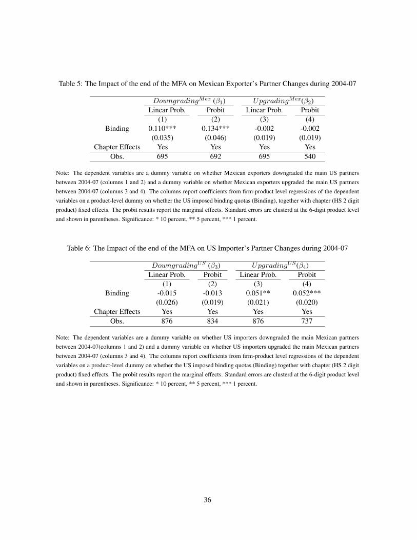
Table 5: The Impact of the end of the MFA on Mexican Exporter’s Partner Changes during 2004-07

Downgrading

Mex (�1) Upgrading

Mex(�2)Linear Prob. Probit Linear Prob. Probit

(1) (2) (3) (4)Binding 0.110*** 0.134*** -0.002 -0.002

(0.035) (0.046) (0.019) (0.019)Chapter Effects Yes Yes Yes Yes

Obs. 695 692 695 540

Note: The dependent variables are a dummy variable on whether Mexican exporters downgraded the main US partnersbetween 2004-07 (columns 1 and 2) and a dummy variable on whether Mexican exporters upgraded the main US partnersbetween 2004-07 (columns 3 and 4). The columns report coefficients from firm-product level regressions of the dependentvariables on a product-level dummy on whether the US imposed binding quotas (Binding), together with chapter (HS 2 digitproduct) fixed effects. The probit results report the marginal effects. Standard errors are clusterd at the 6-digit product leveland shown in parentheses. Significance: * 10 percent, ** 5 percent, *** 1 percent.

Table 6: The Impact of the end of the MFA on US Importer’s Partner Changes during 2004-07

Downgrading

US (�3) Upgrading

US(�4)Linear Prob. Probit Linear Prob. Probit

(1) (2) (3) (4)Binding -0.015 -0.013 0.051** 0.052***

(0.026) (0.019) (0.021) (0.020)Chapter Effects Yes Yes Yes Yes

Obs. 876 834 876 737

Note: The dependent variables are a dummy variable on whether US importers downgraded the main Mexican partnersbetween 2004-07(columns 1 and 2) and a dummy variable on whether US importers upgraded the main Mexican partnersbetween 2004-07 (columns 3 and 4). The columns report coefficients from firm-product level regressions of the dependentvariables on a product-level dummy on whether the US imposed binding quotas (Binding) together with chapter (HS 2 digitproduct) fixed effects. The probit results report the marginal effects. Standard errors are clusterd at the 6-digit product leveland shown in parentheses. Significance: * 10 percent, ** 5 percent, *** 1 percent.

36

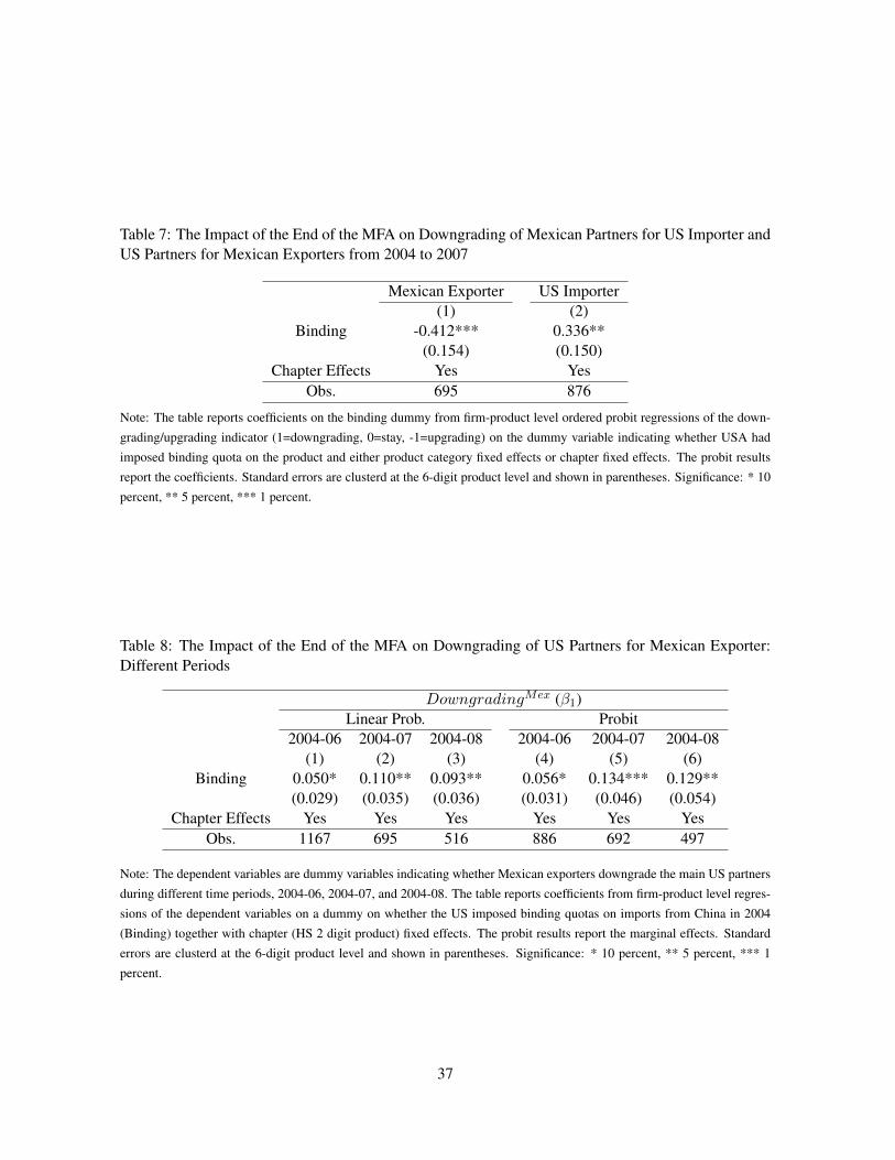
Table 7: The Impact of the End of the MFA on Downgrading of Mexican Partners for US Importer andUS Partners for Mexican Exporters from 2004 to 2007

Mexican Exporter US Importer(1) (2)

Binding -0.412*** 0.336**(0.154) (0.150)

Chapter Effects Yes YesObs. 695 876

Note: The table reports coefficients on the binding dummy from firm-product level ordered probit regressions of the down-grading/upgrading indicator (1=downgrading, 0=stay, -1=upgrading) on the dummy variable indicating whether USA hadimposed binding quota on the product and either product category fixed effects or chapter fixed effects. The probit resultsreport the coefficients. Standard errors are clusterd at the 6-digit product level and shown in parentheses. Significance: * 10percent, ** 5 percent, *** 1 percent.

Table 8: The Impact of the End of the MFA on Downgrading of US Partners for Mexican Exporter:Different Periods

Downgrading

Mex (�1)Linear Prob. Probit

2004-06 2004-07 2004-08 2004-06 2004-07 2004-08(1) (2) (3) (4) (5) (6)

Binding 0.050* 0.110** 0.093** 0.056* 0.134*** 0.129**(0.029) (0.035) (0.036) (0.031) (0.046) (0.054)

Chapter Effects Yes Yes Yes Yes Yes YesObs. 1167 695 516 886 692 497

Note: The dependent variables are dummy variables indicating whether Mexican exporters downgrade the main US partnersduring different time periods, 2004-06, 2004-07, and 2004-08. The table reports coefficients from firm-product level regres-sions of the dependent variables on a dummy on whether the US imposed binding quotas on imports from China in 2004(Binding) together with chapter (HS 2 digit product) fixed effects. The probit results report the marginal effects. Standarderrors are clusterd at the 6-digit product level and shown in parentheses. Significance: * 10 percent, ** 5 percent, *** 1percent.

37

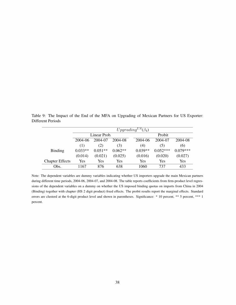
Table 9: The Impact of the End of the MFA on Upgrading of Mexican Partners for US Exporter:Different Periods

Upgrading

US(�4)Linear Prob. Probit

2004-06 2004-07 2004-08 2004-06 2004-07 2004-08(1) (2) (3) (4) (5) (6)

Binding 0.033** 0.051** 0.062** 0.039** 0.052*** 0.079***(0.014) (0.021) (0.025) (0.016) (0.020) (0.027)

Chapter Effects Yes Yes Yes Yes Yes YesObs. 1167 876 638 1060 737 433

Note: The dependent variables are dummy variables indicating whether US importers upgrade the main Mexican partnersduring different time periods, 2004-06, 2004-07, and 2004-08. The table reports coefficients from firm-product level regres-sions of the dependent variables on a dummy on whether the US imposed binding quotas on imports from China in 2004(Binding) together with chapter (HS 2 digit product) fixed effects. The probit results report the marginal effects. Standarderrors are clusterd at the 6-digit product level and shown in parentheses. Significance: * 10 percent, ** 5 percent, *** 1percent.

38

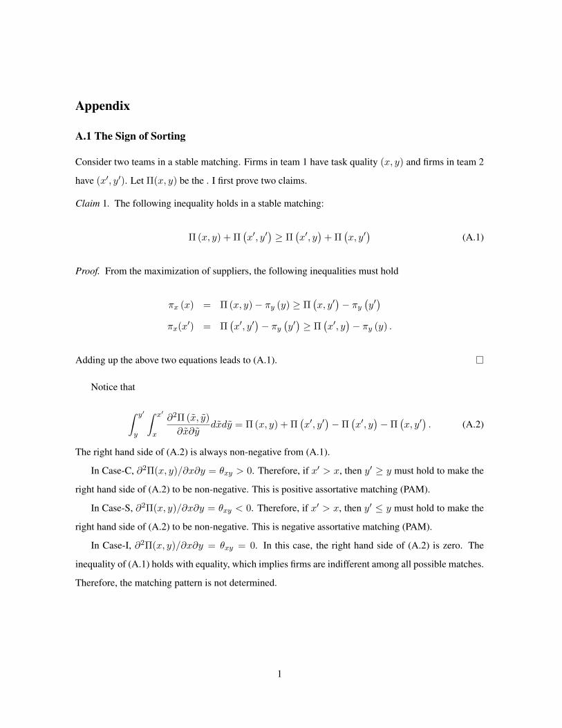
Appendix

A.1 The Sign of Sorting

Consider two teams in a stable matching. Firms in team 1 have task quality (x, y) and firms in team 2

have (x

0, y

0). Let ⇧(x, y) be the . I first prove two claims.

Claim 1. The following inequality holds in a stable matching:

⇧ (x, y) +⇧

�x

0, y

0� � ⇧

�x

0, y

�+⇧

�x, y

0� (A.1)

Proof. From the maximization of suppliers, the following inequalities must hold

⇡

x

(x) = ⇧ (x, y)� ⇡

y

(y) � ⇧

�x, y

0�� ⇡

y

�y

0�

⇡

x

(x

0) = ⇧

�x

0, y

0�� ⇡

y

�y

0� � ⇧

�x

0, y

�� ⇡

y

(y) .

Adding up the above two equations leads to (A.1).

Notice that

ˆy

0

y

ˆx

0

x

@

2⇧ (x, y)

@x@y

dxdy = ⇧ (x, y) +⇧

�x

0, y

0��⇧

�x

0, y

��⇧

�x, y

0�. (A.2)

The right hand side of (A.2) is always non-negative from (A.1).

In Case-C, @2⇧(x, y)/@x@y = ✓

xy

> 0. Therefore, if x0 > x, then y

0 � y must hold to make the

right hand side of (A.2) to be non-negative. This is positive assortative matching (PAM).

In Case-S, @2⇧(x, y)/@x@y = ✓

xy

< 0. Therefore, if x0 > x, then y

0 y must hold to make the

right hand side of (A.2) to be non-negative. This is negative assortative matching (PAM).

In Case-I, @2⇧(x, y)/@x@y = ✓

xy

= 0. In this case, the right hand side of (A.2) is zero. The

inequality of (A.1) holds with equality, which implies firms are indifferent among all possible matches.

Therefore, the matching pattern is not determined.

1