Assimilation of HF Radar Data into Coastal Wave Models

NERC-funded PhD work also supervised byClive W Anderson (University of Sheffield)

Judith Wolf (Proudman Oceanographic Laboratory)

Lee Siddons and Lucy Wyatt

Department of Applied Mathematics

University of Sheffield, UK

Overview

• OSCR HF radar at Holderness

• SWAN Wave Model

• Data Assimilation and Algorithms

• Results

• Future Work

Surface current Wind direction

OSCR measurements

Wave height and peak direction

Peak wave period and direction

Energy spectrum m2/Hz

Mean direction spectrum

Directional frequency spectrum m2/Hz/rad

OSCR

buoy

OSCR wind direction

Wave Modelling

SWAN (Simulating WAves Nearshore)• The Action Balance equation:

• A is the action that is a function of frequency and direction i.e.

• C is the wave group velocity in relevant direction.• S is the forcing to the system. Winds, non-linear

interactions etc.

inyA

yxA

xtA SCC

See Holthuijsen L. H. et al (1999)

)()( fEfAf

SWAN Application to Holderness

Boundary DataBoundary Data

Action

1.2km

1.2km

Data Assimilation

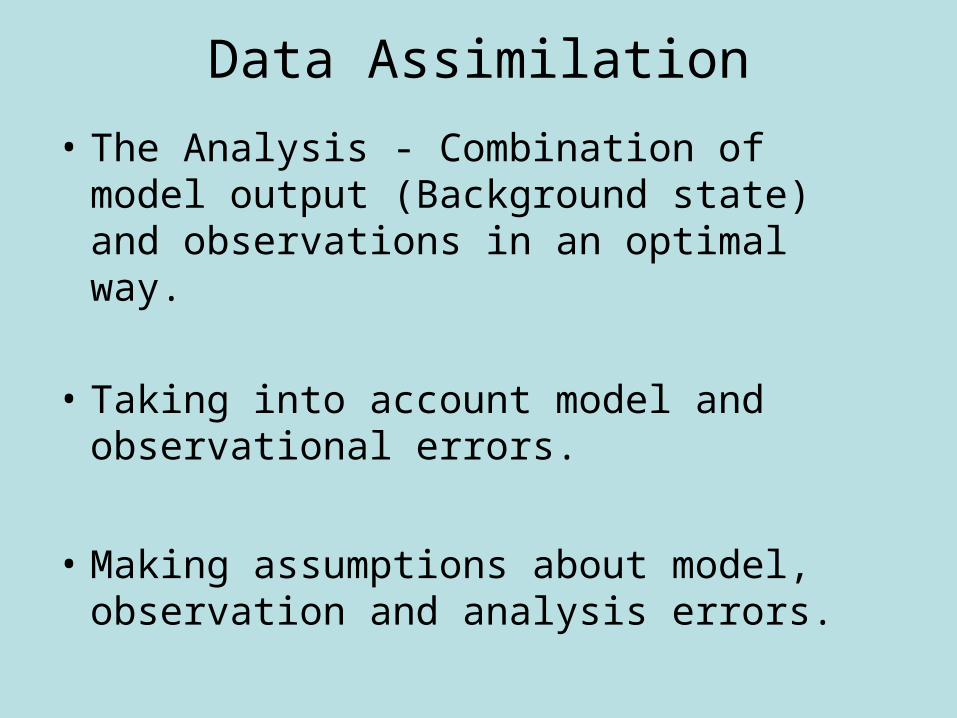
• The Analysis - Combination of model output (Background state) and observations in an optimal way.

• Taking into account model and observational errors.

• Making assumptions about model, observation and analysis errors.

Data Assimilation Formulation

000

111

11

bt

ktk

tk

ktk

tk

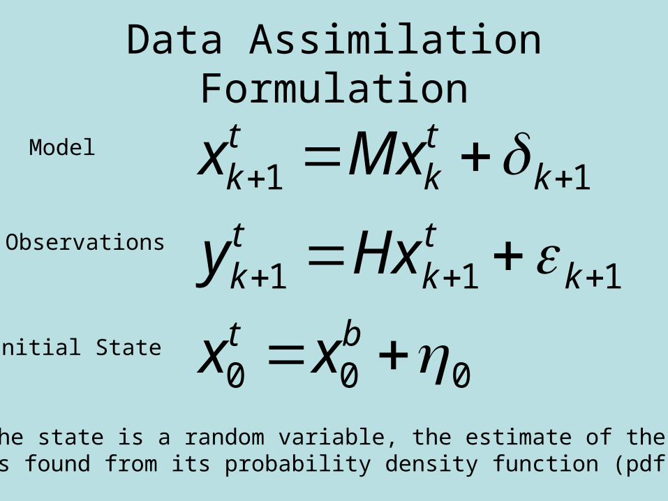
xx

Hxy

MxxModel

Observations

Initial State

Since the state is a random variable, the estimate of the state is found from its probability density function (pdf).

The State of the Ocean The state of the ocean is often described in terms of a few wave parameters, for example: • Significant Wave Height Hs

• Mean wave period T1

These are the state variables used in our assimilations

ddffEHs ,*4

dfdfEf

dfdfE

MT

f )(

)(11

Assimilation AlgorithmsThere are two main approaches of assimilation.

Sequential Assimilation

Only considers observations from the past and to the time of the analysis. Some examples of sequential algorithms are:

• Optimal interpolation• Kalman Filters

Variational Assimilation

Observations from the future can be used at the time of the analysis.Some examples of variational algorithms are:

• Three-dimensional variational assimilation – 3DVAR• Four-dimensional variational assimilation – 4DVAR

The Kalman Filter

)( bkkk

bk

ak HxyKxx

][ Tkk

ak

akkk

eeEP

xxe

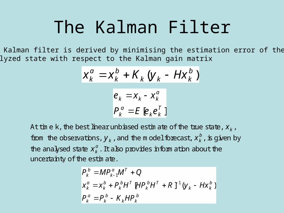
The Kalman filter is derived by minimising the estimation error of the analyzed state with respect to the Kalman gain matrix

bkk

bk

ak

bkk

Tbk

Tbk

bk

ak

Tak

bk

HPKPP

HxyRHHPHPxx

QMMPP

)(][ 1

1

At time k, the best linear unbiased estimate of the true state, kx ,

from the observations, ky , and the model forecast, bkx , is given by

the analysed state akx . It also provides information about the

uncertainty of the estimate.

Variational Assimilation

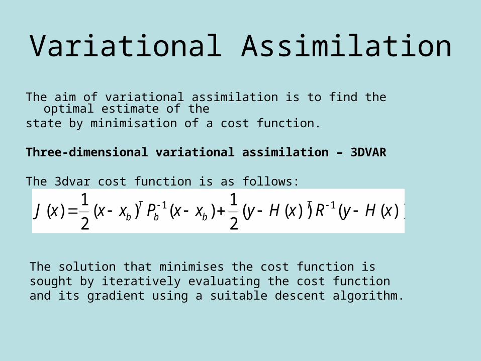
The aim of variational assimilation is to find the optimal estimate of thestate by minimisation of a cost function.

Three-dimensional variational assimilation – 3DVAR

The 3dvar cost function is as follows:

))(())((2

1)()(

2

1)( 11 xHyRxHyxxPxxxJ T

bbT

b

The solution that minimises the cost function is sought by iteratively evaluating the cost function and its gradient using a suitable descent algorithm.

Ensemble Kalman Filter (EnKF)

• EnKF introduced by Evensen - to avoid the computational load associated with

• Sequential method where the error statistics are predicted using Monte Carlo or ensemble integration.

• An ensemble of model states in integrated forward in time and statistical information is calculated from the ensemble.

QMMPP Tak

bk 1

Assimilation with Ideal Data

Before assimilating radar data, thealgorithms have been validated usingsimulated data.

– SWAN is used to generate a ‘true’ state.– Model errors are assumed to be uniform over

the grid and equal to background uncertainty estimated from buoy data.

– Radar measurements are assumed to be available at all sites and errors also uniform.

Results for Simulated Case - 3DVAR

Results for Simulated Case - ENKF

Performance Error Statistics

Scheme MSE Hs MSE Tm

No Assimilation 5.26 * 10-3 6.57 * 10-2

3DVAR 2.679 * 10-3 2.209 * 10-2

Ens_OI 2.709 * 10-3 2.267 * 10-2

ENKF-16 1.05 * 10-3 2.45 * 10-2

Assimilation with Real Data ENS-OI

Assimilation with Real Data EnKF

Assimilation of Band Parameters

• Assimilation of Hs and Tm in the following frequency bands.

Band 1 = 0.03Hz - 0.1Hz

Band 2 = 0.1Hz - 0.2Hz

Band 3 = 0.2Hz - 0.3Hz

Band 4 = 0.3Hz - 0.4Hz

Performance Error Statistics for Test Case Assimilation of Band Parameters

Scheme B1 Hs *10-3

B1 Tm *10-3

B2 Hs *10-3

B2 Tm *10-3

B3 Hs *10-3

B3 Tm *10-3

B4 Hs *10-3

B4 Tm *10-3

No Assimilation

0.16 0.18 11.9 12.0 5.8 4.5 16.3 0.16

3DVAR 0.16 0.13 6.8 6.7 3.6 2.5 8.2 0.17

Ens-OI 0.16 0.14 6.7 6.8 3.7 2.6 8.7 0.16

ENKF-16 0.02 0.15 0.7 3.5 3.1 1.8 3.6 0.29

Assimilation with Real Data 3DVAR

Assimilation with Real Data EnKF

Future Work

• Re-estimate model and radar errors to use in the assimilation schemes.

• Perform a probability sensitivity analysis on the model to find model sensitivities.

• Extend range of assimilated parameters e.g. by using partitioned directional spectra

Energy spectrum m2/Hz

Mean direction spectrum

Directional frequency spectrum m2/Hz/rad

OSCR

buoy

OSCR wind direction