Assignment 01fac.ksu.edu.sa/.../files/Lecture19_DigitalFilters01.docx · Web viewfor 20 samples using MATLAB. Solution A MATLAB program to compute the system response for 20 samples

CEN352 Digital Signal Processing by Dr. Anwar M. Mirza

Lecture No. 19Date: November, 2012

Digital FiltersAims and Objectives

Design filters that have specified frequency characteristics.Analyze frequency selective filters in the z-transform domain.Apply windowing on a signal and explain how it improves the transform properties (some part of this has already been covered in Lecture 11 (Sec. 4.3, Li Tan’s Book).Be able to design, analyze and implement filters in MATLAB.

Department of Computer EngineeringCollege of Computer & Information Sciences, King Saud University

Ar Riyadh, Kingdom of Saudi Arabia



What is Filtering?





The term “Filter” is commonly used to describe“something that holds back elements or modifies the appearance of the contents passing through it”.

Examples could be ofA porous material (such as paper or sand) through which gas or liquid is passed to separate the particles that are present in the gas or liquid. “Air-filters” and “oil-filters” are examples of such filters as used in automobiles.A transparent material (such as colored glass) that absorbs light of certain wavelengths or colors selectively and is used to modify light that reaches the photographic material.A device or material for suppressing or minimizing waves or oscillations of certain frequencies (as of electricity, light or sound).



An LTI System

Digital Input Digital Output



1. The Difference Equation and the Digital Filtering

Consider a DSP system in the form of an LTI system as shown in the figure below

The relationship between its input and output can be expressed in the form of a difference equation as,

y (n )=b0 x (n )+b1 x (n−1 )+…+bM x (n−M )

−a1 y (n−1 )−a2 y (n−2 )−…−aN y (n−N ) (1)

whereb i ,0≤i ≤M anda j ,1≤ j ≤N represent the coefficients of the system andn is the time index. This equation can also be written as

y (n )=∑i=0

M

bi x (n−i )−∑j=1

N

a j y (n− j ) (2)





The equation shows that the current value of the output y (n ) depends on the currentx (n ) and past valuesx (n−1 ) , x (n−2 ) ,…, x (n−M ) of the input as well as the past valuesy (n−1 ) , y (n−2 ) ,…, y (n−N ) of the output.

We have already seen that a system expressed in this form of difference equation fulfills the conditions of linearity, time-invariance and causality.

If the initial conditions are given, the system output (i.e. time response), y (n ), can be obtained recursively (illustrated below by the examples). This process is called digital filtering.

Example 1

Compute the system output

y (n )=0.5 y (n−2 )+x (n−1)

for the first four samples using the following initial conditions

(a) Initial conditions:y (−2 )=1 , y (−1 )=0 , x (−1 )=−1, and input x (n )=(0.5 )nu(n).(b) Zero initial conditions:y (−2 )=0 , y (−1 )=0 , x (−1 )=0, and input x (n )=(0.5 )nu(n).

Solution

(a) Settingn=0, and using the initial conditions, we obtain the input and output as

x (0 )=(0.5 )0u (0 )=1y (0 )=0.5 y (−2 )+x (−1 )=0.5×1−1=−0.5

Settingn=1, and using the initial conditions, we obtain the input and output asx (1 )=(0.5 )1u (1 )=0.5y (1 )=0.5 y (−1 )+ x (0 )=0.5×0+1=1.0

Settingn=2, and using the past values of the input and output,





x (2 )=(0.5 )2u (2 )=0.25y (2 )=0.5 y (0 )+x (1 )=0.5× (−0.5 )+0.5=0.25

Settingn=3, and using the past values of the input and output,x (3 )=(0.5 )3u (1 )=0.125y (3 )=0.5 y (1 )+x (2 )=0.5×1+0.25=0.75

Clearly, it can be seen that the further value of the output can be obtained recursively.

(b) Settingn=0, and using the initial conditions, we obtain the input and output as

x (0 )=(0.5 )0u (0 )=1y (0 )=0.5 y (−2 )+x (−1 )=0.5×0+0=0

Settingn=1, and using the initial conditions, we obtain the input and output asx (1 )=(0.5 )1u (1 )=0.5y (1 )=0.5 y (−1 )+ x (0 )=0.5×0+1=1.0



Clearly, it can be seen that the further value of the output can be obtained recursively.

Example 2

Compute the DSP system output

y (n )=2 x (n )−4 x (n−1 )−0.5 y (n−1 )− y (n−2)





with the initial conditionsy (−2 )=1 , y (−1 )=0 , x (−1 )=−1, and input x (n )=(0.8 )nu(n).

(a) Compute the system response y (n ) for 20 samples using MATLAB.

Solution

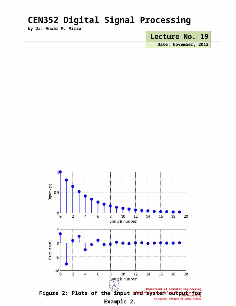
A MATLAB program to compute the system response for 20 samples is given below along with the corresponding output shown in graphical form.

% Example 2%% Compute the response y(n) of a DSP system expressed by% y(n)=2x(n)-4x(n-1)-0.5y(n-1)-y(n-2)% for the first 20 samples. Initial conditions are% y(-2)=1, y(-1)=0, x(-1)=-1 and the system input is% x(n)=(0.8)^n*u(n).% % Initialize the input and output vectorsxi = [0 -1]; % for n=-2 and n=-1yi = [1 0]; % for n=-2 and n=-1 % Compute time indicesn = 0:1:19;% Compute the input samples x(n) for these time instants nx = (0.8).^n;% Include the initial values of input into this vectorx = [xi x]; % Now compute the system responsey = []; % an empty vectory = [yi y]; % after including the initial conditions% compute y(n) recursivelyfor k = 3:1:22 r = 2*x(k-2)-4*x(k-1)-0.5*y(k-1)-0.5*y(k-2); y = [y r];end subplot(2,1,1), stem(n,x(3:22),'filled','LineWidth',2), grid onxlabel('Sample number'); ylabel('Input x(n)');subplot(2,1,2), stem(n,y(3:22),'filled','LineWidth',2), grid onxlabel('Sample number'); ylabel('Output x(n)');





There are two MATLAB functions (syntax given below), that can used to perform this filtering process:

Zi = filtic(B, A, Yi, Xi)

y = filter(B, A, x, Zi)

where B and A are vectors for the coefficients given as

0 2 4 6 8 10 12 14 16 18 200

0.5

1

Sample number

Inpu

t x(n

)

0 2 4 6 8 10 12 14 16 18 20-10

-5

0

5

Sample number

Out

put x

(n)

Figure 2: Plots of the input and system output for Example 2.





A=[1a1a2…aN ] and B=[b0b1b2…bM ]

Xi and Yi are the vectors containing the initial conditions. Also x, y are the input and system output vectors.

The function filtic is used to obtain the initial states required by the second function filter. The function filter is based on the direct-form II realization to implement a digital filter from its difference equation form. This will be studied in a coming lecture.

The following MATLAB code, illustrates how to solve Example 1, using filtic and filter MATLAB functions.

These are the same results as obtained in Example 1.

2. The Difference Equation and the Transfer Function

From Equation 1, we have

y (n )=b0 x (n )+b1 x (n−1 )+…+bM x (n−M )

>> B = [0 1];>> A = [1 0 -0.5];>> Xi = [-1 0];>> Yi = [0 1];>> Zi = filtic(B, A, Yi, Xi);>> n = 0:3;>> x = (0.5).^n;>> y = filter(B, A, x, Zi)

y =

-0.5000 1.0000 0.2500 0.7500





−a1 y (n−1 )−a2 y (n−2 )−…−aN y (n−N )

Assuming that all initial conditions for this system are zero, we take the z-transform of both sides to get

Y ( z )=b0X ( z )+b1 z−1X ( z )+…+bM z

−M X ( z )

−a1 z−1Y ( z )−a2 z

−2Y ( z)−…−aN z−NY ( z ) (3)

We have made use of the shift-theorem in the above equation. Rearranging, we obtain

H ( z )=Y ( z )X (z )

=b0+b1 z

−1+…+bM z−M

1+a1 z−1+…+aN z

−N =B ( z )A ( z ) (4)

whereH ( z ) is defined as the z-transfer function with its numerator and denominator polynomials given by

B (z )=b0+b1 z−1+…+bM z

−M(5)

A ( z )=1+a1 z−1+…+aN z

−N (6)

It can clearly be notices that the z-tranfer function is the ratio of the z-transform of the output with the z-transform of the input. This can diagrammatically be shown as

The z-transfer function can be used to determine the stability and frequency response of the digital filter.

Example 3

A DSP system is described by the following difference equation

Digital Filter Transfer function

z-transform Input z-transform Output





y (n )=x (n )−x (n−2 )−1.3 y (n−1 )−0.36 y (n−2)

Find the z-transfer functionH ( z ), the denominator polynomialA ( z ), and the numerator polynomialB (z ).

Solution

Taking the z-transform of both sides of the given difference equation, and using the shift-theorem, we get

Y ( z )=X ( z )−z−2 X ( z )−1.3 z−1Y ( z )−0.36 z−2Y (z)

It can also be written as

Y ( z )+1.3 z−1Y (z )+0.36 z−2Y (z )=X ( z )−z−2 X (z )

Y ( z ) (1+1.3 z−1+0.36 z−2 )=X ( z ) (1−z−2 )

Y ( z )X ( z )

=(1−z−2 )

(1+1.3 z−1+0.36 z−2 )

The transfer function, is therefore, given by

H ( z )=Y( z )

X (z )=

(1−z−2)(1+1.3 z−1+0.36 z−2 )

The denominator and numerator polynomials are

A ( z )=1+1.3 z−1+0.36 z−2

B (z )=1−z−2

Example 4

A digital system is described by the following difference equation

y (n )=x (n )−0.5 x (n−1 )+0.36 x (n−2)





Find the z-transfer functionH ( z ), the denominator polynomialA ( z ), and the numerator polynomialB (z ).

Solution

Taking the z-transform of both sides of the given difference equation, and using the shift-theorem, we get

Y ( z )=X ( z )−0.5 z−1 X (z )+0.36 z−2 X (z )

It can also be written as

Y ( z )=X ( z ) (1−0.5 z−1+0.36 z−2 )

Y ( z )X ( z )

= 1(1−0.5 z−1+0.36 z−2 )

The transfer function, is therefore, given by

H ( z )=Y ( z )X (z )

= 1(1−0.5z−1+0.36 z−2 )

The denominator and numerator polynomials are

A ( z )=1−0.5 z−1+0.36 z−2

B (z )=1

In some DSP applications, the given transfer function of a digital system can be converted into a difference equation for DSP implementation. The following example illustrates this procedure.

Example 5

Convert each of the following transfer functions into its difference equation

(a) H ( z )= z2−1z2+1.3 z+0.36





(b)H ( z )= z2−0.5 z+0.36

z2

Solution

Part (a): We first divide the numerator and denominator byz2 to obtain the transfer function whose numerator and the denominator polynomials have the negative powers ofz, it follows that

H ( z )=( z2−1 )/ z2

( z2+1.3 z+0.36 ) /z2=

(1−z−2 )(1+1.3 z−1+0.36 z−2 )

According to the definition of the transfer function

H ( z )=Y ( z )X (z )

Therefore, in this case,

Y ( z )X ( z )

=(1−z−2 )

(1+1.3 z−1+0.36 z−2 )

Cross multiplication gives

(1+1.3 z−1+0.36 z−2 )Y ( z )=(1−z−2 ) X ( z )

Y ( z )+1.3 z−1Y (z )+0.36 z−2Y (z )=X ( z )−z−2 X (z )

Applying the inverse z-transform and applying the shift-theorem

y (n )+1.3 y (n−1 )+0.36 y (n−2 )=x (n )−x (n−2 )

This equation can be re-arranged to give the required difference equation for the DSP system, as

y (n )=x (n )−x (n−2 )−1.3 y (n−1 )−0.36 y (n−2 )





Part (b): In this case also, we first divide the numerator and denominator byz2 to obtain the transfer function whose numerator and the denominator polynomials have the negative powers ofz, it follows that

H ( z )=( z2−0.5 z+0.36 )/ z2

( z2 )/ z2=

(1−0.5 z−1+0.36 z−2)1

According to the definition of the transfer function

H ( z )=Y ( z )X (z )


Y ( z )X ( z )

=(1−0.5 z−1+0.36 z−2 )

It can be written as

Y ( z )=(1−0.5 z−1+0.36 z−2 ) X ( z )

Y ( z )=X ( z )−0.5 z−1 X (z )+0.36 z−2 X ( z )

Applying the inverse z-transform and applying the shift-theorem

y (n )=x (n )−0.5x (n−1 )+0.36x (n−2 )

This is the required difference equation for the DSP system.

Transfer Function in Pole-Zero Form





From Equation 4, we know that the transfer function for a digital filter can be written as

H ( z )=Y ( z )X (z )

=b0+b1 z

−1+…+bM z−M

1+a1 z−1+…+aN z

−N =B ( z )A ( z )

The numeratorB (z ) and the denominatorA ( z ) polynomials of the transfer functionH ( z ) can be factorized. The transfer functionH ( z ) can therefore, be written in its pole-zero form as

H ( z )=b0 ( z−z1 ) ( z−z2)… ( z− zM )( z−p1 ) ( z−p2 )… ( z−pN )

(7)

where the zerosz i and polesp j can be found by solving (finding the roots of) the polynomial equations

zM+( b1b0 ) zM−1+…+( bMb0 )=0a1 z

N+a2 zN−1+…+bN=0

This is explained with the following example.

Example 6

Given the following transfer function

H ( z )=(1−z−2 )

(1+1.3 z−1+0.36 z−2 )

Convert it into its pole-zero form.

Solution

We first multiply the numerator and denominator byz2 to obtain the transfer function whose numerator and the denominator polynomials have the positive powers ofz, as follows





H ( z )=(1−z−2 ) z2

(1+1.3 z−1+0.36 z−2 ) z2= z2−1z2+1.3 z+0.36

Putting the numerator polynomial equal to zero and then finding the roots, gives us the zeros of the transfer function,

z2−1=0

( z−1 )(z+1)=0

Therefore, we getz1=1 andz2=−1 as the roots.

Now, setting the denominator polynomial equal to zero and find the roots, gives us the poles of the transfer function,

z2+1.3 z+0.36=0

z=−1.3±√(1.3 )2−4 (1 )(0.36)2(1)

=−1.3±√1.69−1.442

=−1.3±√0.252

=−1.3±0.52

=−0.4 ,−0.9

Therefore, the poles arep1=−0.4 andp21=−0.9. The transfer function can now be written in the pole-zero form as

H ( z )= ( z−1 ) ( z+1 )(z+0.4 ) ( z+0.9 )

Impusle Response, Step Response and System Response

Example 6.7

Given a transfer function depicting a DSP system

H ( z )= z+1z−0.5





Determine

(a) The impulse responseh (n )

(b) The step responsey (n ), and(c) The system responsey (n ), if the input is given asx (n )=(0.25 )nu(n).

Solution

Part (a): In this casex (n )=δ (n ), thusX ( z )=1. As

H ( z )=Y ( z )X (z )

Therefore, in this case, the z-transform of the output is equal to the transfer function:

H ( z )=Y ( z )

By taking the inverse z-transform of the transfer function we can find out the unit impulse responseh (n ) of the system. The transfer function can be written as

H ( z )z

= z+1z ( z−0.5 )

This can further be written in the form of partial fractions as

H ( z )z

= Az+ B

( z−0.5 )

where

A= z+1( z−0.5 )|z=0= 0+1

(0−0.5 )=−2

B= z+1z |

z=0.5=0.5+1

0.5=3

Thus we have





H ( z )z

=−2z

+ 3( z−0.5 )

Or

H ( z )=−2+ 3 z( z−0.5 )

Taking inverse z-transform of both sides (and using Table 5.1), we get

h (n )=−2δ (n )+3 (0.5 )nu (n )

which is the required impulse response of the system.

Part (b): In this casex (n )=u (n ), thusX ( z )= zz−1 . As

H ( z )=Y ( z )X (z )


Y ( z )=H ( z )X ( z )= ( z+1 )( z−0.5 )

z( z−1 )


Y ( z )z

= z+1( z−0.5 ) ( z−1 )


Y ( z )z

= A( z−0.5 )

+ B(z−1 )

where

A= z+1( z−1 )|z=0.5= 0.5+1

(0.5−1 )=−3





B= z+1( z−0.5 )|z=1= 1+1

1−0.5=4

Thus we have

Y ( z )z

= −3( z−0.5 )

+ 4(z−1 )

Or

Y ( z )= −3 z(z−0.5 )

+ 4 z( z−1 )


y (n )=−3 (0.5 )nu (n )+4u (n )

which is the required step response of the system.

Part (c): In this casex (n )=(0.25 )nu (n ), thus from Table 5.1,X ( z )= zz−0.25 . As

H ( z )=Y ( z )X (z )


Y ( z )=H ( z )X ( z )= ( z+1 )( z−0.5 )

z( z−0.25 )


Y ( z )z

= z+1( z−0.5 ) ( z−0.25 )


Y ( z )z

= A( z−0.5 )

+ B(z−0.25 )

where





A= z+1( z−0.25 )|z=0.5= 0.5+1

(0.5−0.25 )= 1.50.25

=6

B= z+1( z−0.5 )|z=0.25= 0.25+1

0.25−0.5= 1.25

−0.25=−5

Thus we have

Y ( z )z

= 6( z−0.5 )

+ −5(z−0.25 )

Or

Y ( z )= 6 z(z−0.5 )

− 5 z( z−0.25 )


y (n )=6 (0.5 )nu (n )+5 (0.25 )nu (n )

which is the required system response.

Table 5.1 Table of z-transform pairs (for causal sequences)

Line No.

Signalx (n ) ,n≥0

z-TransformZ (x (n ) )=X (z)

Region of Convergence

1 x (n) ∑n=0

∞

x (n ) z−n

2 δ (n) 1 Entire z-plane

3 au(n)azz−1 |z|>1

4 nu(n)z

( z−1 )2|z|>1

5 n2u(n)z( z+1)( z−1 )3

|z|>1

6 anu(n)zz−a |z|>|a|





7 e−nau(n)z

z−e−a|z|>e−a

8 nanu(n)az

( z−a )2|z|>|a|

9 sin (an )u(n)z sin (a )

z2−2 z cos (a )+1|z|>|1|

10 cos ( an )u (n)z ( z−cos (a ) )

z2−2 z cos (a )+1|z|>|1|

11 ansin (bn )u(n)[a sin (b ) ] z

z2−[2acos (b ) ] z+a2|z|>|a|

12 ancos (bn )u (n)z [z−acos (b ) ]

z2−[2acos (b ) ] z+a2|z|>|a|

13 e−an sin (bn )u (n)[e−a sin (b ) ] z

z2−[2e−acos (b ) ] z+e−2a |z|>e−a

14 e−an cos (bn )u(n)z [ z−e−a cos (b ) ]

z2−[2e−acos (b ) ] z+e−2a |z|>e−a

152|A||P|ncos (nθ+ϕ )u (n ) whereP andA are complex constants defined byP=|P|∠θ, A=|A|∠ϕ

Azz−P

+ A ¿zz−P¿

Shift Theorem: Z (x (n−m ) )=z−mZ (x (n ) )



Documents

Assignment 01fac.ksu.edu.sa/.../files/Lecture19_DigitalFilters01.docx · Web viewfor 20 samples using MATLAB. Solution A MATLAB program to compute the system response for 20 samples