Asset Specificity of Non-Financial Firms*

Amir Kermani1 and Yueran Ma2

1Berkeley Haas2Chicago Booth

August 10, 2020

Abstract

We study asset specificity of US non-financial firms using a new dataset on the

liquidation recovery rates of all major asset categories across industries. First, we find

a high average level of asset specificity. Second, across industries, physical attributes

of assets account for substantial variations in liquidation recovery rates. Over time,

macroeconomic and industry conditions have the most impact when assets are not firm-

specific. Third, higher asset specificity is associated with less disinvestment, greater

investment response to uncertainty, and more Q dispersion, consistent with theories

of investment irreversibility. Finally, rising intangibles have had a limited impact on

firms’ liquidation values.

JEL: E22, E32, G31, G33.Key words: Asset specificity; Investment irreversibility; Rising intangibles.

*We thank Douglas Baird, Effi Benmelech, Ricardo Caballero, Larry Christiano, Emanuele Colonnelli,Nicolas Crouzet, Marty Eichenbaum, Emmanuel Farhi, Murray Frank, Victoria Ivashina, Steve Kaplan,Anya Kleymenova, Christian vom Lehn, Jacob Leshno, Lisa Yao Liu, Max Maksimovic, Akhil Mathew,Michael Minnis, Justin Murfin, Gordon Phillips, Jose Scheinkman, Andrei Shleifer, Alp Simsek, JamesTraina, Rob Vishny, Wei Wang, Michael Weber, Tom Winberry, Chunhui Yuan, seminar participants atBocconi, Chicago Booth, the Chicago Fed, and conference participants at NBER Summer Institute forvaluable comments and suggestions. We are grateful to finance professionals John Coons and Doug Jungfor sharing their valuable knowledge and insights. We are indebted to Fatin Alia Ali, Leonel Drukker,Bianca He, and Julien Weber for outstanding research assistance. First draft: March 2020. Emails: ker-mani@berkeley.edu, yueran.ma@chicagobooth.edu.

1 Introduction

Asset specificity is a key feature of production activities in practice. As Bertola and

Caballero (1994) articulate, once installed, capital often has “little or no value unless used

in production.” Asset specificity also plays a prominent role in a wide range of economics

research. It can lead to investment irreversibility (Pindyck, 1991; Bertola and Caballero,

1994; Abel and Eberly, 1996), and influence price setting (Woodford, 2005; Altig, Christiano,

Eichenbaum, and Linde, 2011). It may also affect the form of organizations (Williamson,

1981), as well as debt contracting (Shleifer and Vishny, 1992; Kiyotaki and Moore, 1997).

The central challenge for studying asset specificity and its implications is measurement.

What is the value of different assets if they were displaced, separated from current use and

moved to alternative use? Such data has been sparse so far, and secondary market trading

information is only readily available for a limited and selected subset of assets. An important

prior work is Ramey and Shapiro (2001), which collects comprehensive data from auctions of

aerospace manufacturing equipment, and estimates that the transaction value of equipment

is on average 28% of replacement cost. Other studies generally rely on imputations or

indirect proxies such as the prevalence of asset usage across industries (Berger, Ofek, and

Swary, 1996; Almeida and Campello, 2007; Gulen and Ion, 2016; Kim and Kung, 2017).

With the lack of systematic data on the degree of asset specificity, models have also used a

wide range of parameter values.

In this paper, we tackle the challenge by constructing a new dataset that directly mea-

sures asset specificity for all major asset types (e.g., fixed asset, inventory, receivable) and

major industries. We document that assets are highly specific in most industries. We

then investigate the key determinants of variations in asset specificity, including physical

attributes of assets used in different industries (such as mobility, durability, standardiza-

tion/customization), as well as macroeconomic and industry conditions. We finally show

that the data has a wide range of applications. It sheds further light on several aspects of

investment theories; it also informs our understanding of the impact of rising intangibles.

To fix ideas, for each type of asset, we quantify the degree of asset specificity using the

liquidation value relative to the replacement cost, henceforth referred to as the liquidation

recovery rate. This ratio corresponds to the degree of investment irreversibility in a number

of models (Abel and Eberly, 1996; Bloom, 2009). Alternatively, one might also think of

asset specificity defined as the ratio of the value in alternative use relative to the value in

1

current use. The value in current use is unfortunately difficult to assess for each individual

asset category (since a firm has multiple types of assets and one can only observe the market

value of the firm as a whole). To the extent that the value in current use is typically higher

than the replacement cost, this alternative ratio would lead to an even higher degree of

asset specificity. In addition, the nature of the data also implies that it captures the value

from reallocating standalone and separable assets by themselves, not combined with human

capital or organizational capital.1

The first step of our work is to collect data on the liquidation recovery rates of major

types of assets across industries. The most systematic reporting of this information comes

from the liquidation analysis in US Chapter 11 bankruptcy filings, and we hand collect this

data from 2000 to 2016. Specifically, firms in Chapter 11 continue to operate, but are also

required to document the estimated value of their assets if they were to be liquidated in

Chapter 7—in which case the firm would cease operations and liquidate its assets. These

estimates commonly derive from specialist appraisers who perform on-site field examinations

and simulate live liquidations. The large cases typically report in detail the estimated

liquidation recovery rate for each category of asset, such as plant, property, and equipment

(PPE), inventory, receivable, cash, and book intangible. We take the average recovery rate

for each type of asset in a two-digit SIC industry in the baseline analysis to reduce noise,

which currently covers nearly 50 non-financial two-digit SIC industries.

We find that firms’ assets are highly specific on average, but there are meaningful vari-

ations across industries. The industry-level liquidation recovery rate for PPE is 35% on

average, and it ranges from close to 70% for transportation to less than 10% for certain

services. The industry-level liquidation recovery rate for inventory is 44% on average, and

it ranges from about 80% for auto dealers and retailers to less than 20% for restaurants. If

we take the industry-level liquidation recovery rate and estimate the total liquidation value

of firms in Compustat based on their industries and the book value of each type of asset,

we find that the total liquidation value of PPE and working capital combined is 23% of

total book assets for the average firm (and 46% when other assets and all cash are also

included). In addition to the comparison with book values, at the firm level, the estimated

total liquidation value (including all assets and cash) is about 50% of the enterprise value for

the median firm in the Chapter 11 sample, and 33% in Compustat. Overall, non-financial

1If human capital and organizational capital remain, then the value would be akin to the value undercurrent use, rather than the liquidation value (Kiyotaki and Moore, 1997), and the former is much higher.

2

firms’ assets are specialized and the piecemeal value to alternative users tends to be low,

relative to both replacement costs and firm values from current use.

We perform extensive checks about the informativeness of the data. The checks verify

that the liquidation value estimates in our data are consistent with market-based transac-

tions (in settings where such data is available). They also verify that although the liquidation

recovery rate data is most comprehensive for Chapter 11 firms, it is relevant for firms in the

same industry more generally. First, for aerospace manufacturing equipment that Ramey

and Shapiro (2001) study using auctions data, the recovery rate is 28% in their analysis and

32% in our sample. Second, the total liquidation value in our data is comparable to the

total liquidation proceeds in actual Chapter 7 liquidations (unfortunately Chapter 7 cases

offer much less information beyond the total proceeds realized by the trustee).2 Third, the

liquidation recovery rates in our data are also in line with lenders’ benchmarks for non-

financial firms in general, which are 20% to 30% for industrial PPE for instance according

to a large bank. Fourth, we compute the industry-average recovery rates implied by PPE

sales among all Compustat firms, and find them to be similar to PPE liquidation recovery

rates in our data, with a significant positive correlation between the two measures across

industries. Finally, the informativeness of the data is further reflected by its consistency

with the physical attributes of assets used in different industries (measured for all firms in

each industry from separate data sources), and importantly with the investment behavior

of firms overall, which we analyze in the rest of the paper.

The second step of our work is to examine the key determinants of variations in asset

specificity, using PPE liquidation recovery rates as the main example. We begin by studying

the impact of three physical attributes: 1) mobility, measured using the transportation costs

of PPE; 2) durability, measured using the depreciation rate of PPE, since asset reallocation

takes time; and 3) degree of standardization/customization, measured using the average

share of design costs in the production costs of PPE. To construct these measures, we collect

detailed information on the composition of each industry’s asset stock using the fixed asset

tables from the Bureau of Economic Analysis (BEA), as well as transportation costs and

design costs using the BEA’s input-output tables. We show that asset specificity is higher

and liquidation recovery rates are lower when the asset is less mobile, less durable, and more

customized. Indeed, these three attributes can account for around 40% of the variations

2In Chapter 7 cases, it is difficult to calculate the liquidation recovery rate for each type of asset.Assets foreclosed by lenders or abandoned by the trustee are also generally excluded from the reported totalproceeds, which requires additional imputation (Bris, Welch, and Zhu, 2006).

3

in the average PPE recovery rate across industries, despite potential measurement noise.

Moreover, the estimates also imply that if PPE has no transportation cost, no depreciation,

and no customization, the recovery rate would be 100%. Overall, the findings indicate strong

physical foundations for the degree of asset specificity.

We also study the impact of time-varying macroeconomic conditions and industry con-

ditions. We find that their impact on PPE recovery rates is in the direction of theoretical

predictions for the average industry, but could be somewhat weak. However, the impact

tends to be much stronger for industries where a larger share of PPE is not customized to the

firm. In other words, when natural buyers are economy-wide (i.e., vehicles) or industry-wide

(e.g., aircraft, ships, oil and gas equipment), macro and industry conditions are particularly

relevant. When assets are firm-specific and not very useful to others in any case, macro and

industry conditions appear less relevant. We also find that the cross-industry differences in

PPE recovery rates (driven by physical attributes) are not easily offset by cyclical variations.

In addition, the magnitudes shown by the data suggest that while better macroeconomic

conditions and industry conditions could increase liquidation recovery rates (e.g., by five or

ten percentage points), they do not seem to change the overall picture of fairly high asset

specificity in many non-financial industries.

After analyzing the determinants of asset specificity, the third step of our work is to

investigate the implications of asset specificity for firms’ behavior. We start with traditional

investment theories. As observed by a large literature, when asset specificity is higher, it

is more difficult to disinvest and downsize the capital stock: investment is more irreversible

(Pindyck, 1991; Bertola and Caballero, 1994; Abel and Eberly, 1996; Bloom, 2009, 2014).

We first verify that in industries with lower PPE recovery rates, firms have less PPE sales,

in terms of both frequency and dollar amount. We then show that, as predicted by theory,

capital expenditures (i.e., investment in PPE) are more negatively affected by uncertainty

shocks when PPE recovery rates are lower. Indeed, the sensitivity is estimated to become

roughly zero if the PPE recovery rate is 100%. We also find that inventory investment is

sensitive to uncertainty shocks when inventory recovery rates are low, while the estimated

sensitivity is again around zero if the inventory recovery rate is 100%. Furthermore, the

sensitivity of PPE investment to uncertainty is affected by PPE recovery rates, but not by

inventory recovery rates, and vice versa. Our results hold based on direct measurement of re-

covery rates, as well as recovery rates “instrumented” (or “fitted”) using the assets’ physical

attributes. Overall, we find a high level of alignment, both qualitatively and quantitatively,

4

between theoretical predictions and the data.

We also find evidence in line with several other implications of costly capital adjustment

and irreversibility. First, for pricing behavior, we find that industries with higher asset speci-

ficity display more price rigidity, based on price change data from Nakamura and Steinsson

(2008). The results appear consistent with the literature on firm-specific capital and price

stickiness (Woodford, 2005; Altig et al., 2011). Second, for productivity dispersion, we find

that industries with higher asset specificity display more dispersion in Q, in line with the

observations of Eisfeldt and Rampini (2006) and Lanteri (2018). This phenomenon holds

for large firms as well, where liquidation values are not a primary driver of financial frictions

like borrowing constraints (Lian and Ma, 2020), which suggests that asset specificity likely

has its impact through costly adjustment.

In addition to implications for traditional investment theories, our data also has implica-

tions for understanding the impact of rising intangible assets (Corrado, Hulten, and Sichel,

2009; Peters and Taylor, 2017; Crouzet and Eberly, 2019), broadly defined as production

assets without physical presence. They include identifiable intangibles such as software,

patents, usage rights, as well as organizational capital that is not necessarily independently

identifiable. A key concern in recent research is that rising intangibles could decrease firms’

liquidation values, and then tighten borrowing constraints (Giglio and Severo, 2012; Caggese

and Perez-Orive, 2018; Falato, Kadyrzhanova, Sim, and Steri, 2020). We find that the change

in firms’ liquidation values in recent years may not be substantial, for three reasons. First,

as discussed above, physical assets are highly specific to begin with. Second, in many in-

dustries, the average liquidation recovery rates of identifiable intangibles do not appear to

be much lower than those of PPE, in part because reallocating intangibles does not face

transportation costs given their lack of physical presence. Third, industries with a greater

increase in intangibles have been the ones with more specific physical assets in the first

place. Taken together, the aggregate liquidation value among Compustat firms in 2016 is

similar to that in 1996.

It would be natural to ask how asset specificity affects firms’ debt contracts and borrowing

capacity, which we study in detail in a companion paper (Kermani and Ma, 2020). We find

that liquidation values do not affect the total amount of borrowing for large firms and

firms with positive earnings. They do have a significant positive impact on total borrowing

for small firms and firms with negative earnings. Meanwhile, asset specificity does affect

the composition of debt: firms with higher liquidation values have more asset-based debt

5

(lending on the basis of the liquidation value of discrete assets like PPE), while firms with

lower liquidation values have more cash flow-based debt (lending on the basis of cash flows

from firms’ operations) and debt with strong control rights. The results are consistent

with observations in Lian and Ma (2020) about the importance of cash flow-based lending

among non-financial firms. When firms have positive earnings (e.g., most large firms), total

debt capacity is typically driven by earnings-based borrowing constraints, instead of the

liquidation value of discrete assets.

Finally, we connect our data with parameters in models, which have used or estimated

a variety of values for the degree of investment irreversibility or the amount of liquidation

value from physical capital. We hope that our micro data helps inform modeling analyses.

Our work has three main contributions. First, we provide comprehensive data on the

degree of asset specificity across different types of assets and industries. Second, we investi-

gate the effect of physical attributes, as well as macro and industry conditions, on variations

in asset specificity. Third, the granular and quantitative nature of our data allows us to per-

form a rich set of analyses about the implications of asset specificity. Our findings shed light

on the impact of investment irreversibility and rising intangibles. The physical attributes of

assets we measure also allow us to establish these links based on physical foundations.

The paper is organized as follows. Section 2 explains the data collection and presents

basic statistics. Section 3 studies the determinants of asset specificity, including physical at-

tributes as well as macro and industry conditions. Section 4 investigates several implications.

Section 5 summarizes the comparison with parameters in models. Section 6 concludes.

2 Data and Basic Statistics

In this section, we discuss the data and measurement of asset specificity. We collect

data on the liquidation recovery rate—i.e., liquidation value as a fraction of net book value

(historical cost net of depreciation)—of major asset categories (e.g., PPE, inventory, receiv-

able, book intangible) across major industries. The liquidation value estimates represent

proceeds from a typical orderly liquidation process, and provide information about the value

of each type of asset in alternative use. By definition, high asset specificity means limited

value in alternative use, and correspondingly a low liquidation recovery rate. Importantly,

the liquidation value captures the value from reallocating standalone and separable assets

by themselves, not combined with human capital or organizational capital.

6

We normalize the liquidation value using replacement costs, similar to Ramey and

Shapiro (2001). An alternative approach is to normalize the liquidation value using the

value of the asset in current use. Our approach is driven by three main reasons. First, data

on the net book value is available for each type of asset, while the value in current use is

difficult to assess for a particular category of assets. Second, the liquidation value relative

to costs is commonly used in models, which we discuss in more detail in Section 5. Third,

the ratio of the liquidation value relative to costs is, to a large extent, determined by the

inherent attributes of assets used in a given industry (as we further verify in Section 3), and

can be more reliably generalized to firms in the same industry. The ratio of the liquidation

value relative to the value in current use, on the other hand, could depend on each firm’s

managerial quality that affects the denominator. Nonetheless, for the firm as a whole, we

can still provide some information about the ratio of the total liquidation value relative to

the firm’s enterprise value, which we discuss in Section 2.4.

2.1 Data Collection

To systematically measure the degree of asset specificity of non-financial firms, secondary

market transactions data faces a number of challenges. First, such data is available for cer-

tain types of relatively standardized assets (e.g., vehicles, aircraft, construction equipment),

but difficult to obtain for many types of real assets. Second, it is also difficult to know

the pool of assets firms own, in which case one cannot aggregate individual items to an

estimate at the firm level. To overcome these obstacles, a setting with comprehensive re-

porting covering all assets firms own is the liquidation analysis performed in Chapter 11

corporate reorganization. When firms complete Chapter 11, they are required to document

the estimated liquidation value that their assets can obtain if they were to be liquidated in

Chapter 7, where the firm ceases operations and a trustee liquidates its assets (largely piece-

meal with a roughly one year time frame). The estimates generally derive from appraisal

specialist firms, who usually serve as liquidators of real assets as well.3 They perform field

exams and simulate live liquidations to appraise the liquidation value of different types of

assets. They are also commonly responsible for assessing liquidation values for lenders who

lend against particular assets and set borrowing limits accordingly, which follows a similar

3The appraisal firms have extensive knowledge, experience, and historical data about what would be afeasible way to conduct a liquidation: how much can be sold to buyers from primary, secondary, and tertiarymarkets, and at what price, etc.

7

appraisal process.

We hand collect liquidation recovery rate data from disclosure statements of Chapter

11 filings, for US non-financial firms from 2000 to 2016. Specifically, we begin with a

list of bankruptcy filings by public US non-financial firms from New Generation Research

BankruptcyData.Com. We then retrieve the disclosure statements of Chapter 11 cases from

Public Access to Court Electronic Records (PACER) and BankruptcyData.Com.4 The

liquidation analysis typically includes a summary table with the net book value, liquidation

value, and liquidation recovery rate (liquidation value as a fraction of net book value) for

each main category of asset (e.g., PPE, inventory, receivable) and for the entity as a whole,

together with notes that explain in more detail the sources and assumptions of the estimates.

Internet Appendix Figure IA1 shows two examples of the summary tables, from Lyondell

Chemical and Sorenson Communications. Internet Appendix Section IA2 shows the detailed

information behind the summary table for Lyondell Chemical, which includes the procedure

for the estimates and facility-level appraisals for Lyondell’s PPE. We use the midpoint

estimate in the summary table, and the average of low and high scenarios when the midpoint

is not available. We have been able to retrieve liquidation analysis summary tables for 360

cases so far, covering 48 two-digit non-financial SICs.

This data has several advantages. First, as mentioned above, it covers all assets owned

by a firm, instead of only assets with secondary market trading data (which tend to exclude

specialized assets) or are chosen to be sold off, which only include certain types of assets or

may entail selection (Ramey and Shapiro, 2001; Maksimovic and Phillips, 2001; Ottonello,

2018). Second, it shows not just the liquidation value in dollar amounts, but also the recovery

rate, i.e., liquidation value as a fraction of book value. Having recovery rates is important

for comparing specificity across different types of assets, and for constructing specificity

measures more broadly applicable for each industry as we discuss below. Third, the data

includes firms from all major industries in a reasonably standardized format. Finally, relative

to indirect proxies of asset specificity, our data allows for the assessment of the dollar

magnitude (important in many applications such as issues analyzed in Section 4), provides

a uniform metric across different sets of assets (e.g., PPE and inventory), and connects

directly to model parameters (discussed in Section 5).

Our data covers assets owned by firms. Some assets that firms use may be under op-

4When a case has multiple disclosure statements, we use the earliest version. If the information we needis not available in the first version, we then use the latest version.

8

erating lease, instead of being owned. The owned assets within the boundary of the firm

are our primary focus for several reasons. First, real decisions like investment expenditures

capture spending on owned assets. Second, owned assets appear to dominate in quantity in

most industries. Specifically, starting in 2019, a new accounting rule (Accounting Standards

Update 842) requires firms to report the capitalized value of leased (right-of-use) assets and

corresponding operating lease liabilities. Based on the new disclosure, the median ratio of

leased assets to owned assets is about 2% among Compustat firms (the inter-quartile range

is 0% to 5.3%).5 The prevalence of operating leases also appears to be largely an industry

attribute, and industry fixed effects (e.g., two-digit SIC) account for about 30% of R2 in the

variation of the ratio of leased assets to owned assets. The ratio of leased to owned assets

is particularly high for certain retail industries (median above 20% for restaurants, depart-

ment stores, apparel, furniture, hardware, and food stores), modest for airlines and cinemas

(median around 10%),6 and very low (median well below 10%) for most other industries.

2.2 Checks of Data Informativeness

We perform extensive checks to examine the reliability of the data. One might be

concerned that the liquidation values are based on estimates, which may introduce inac-

curacies.7 One might also be concerned that firms in Chapter 11 are special and different

from the typical non-financial firm, because the Chapter 11 restructuring may occur when

the firm, its industry, or the economy experiences unfavorable conditions. This may lead

to lower liquidation values, or distortions in the differences across industries. We examine

these concerns in detail. Our checks verify that the liquidation value estimates in our data

are consistent with market-based outcomes (in settings where such data is available), such

5Another way to estimate the prevalence of operating leases is to calculate assets owned by the twolessor sectors in BEA data, which are 5320 (Rental and Leasing Services and Lessors of Intangible Assets)and 5310 (Real Estate, which includes REITs that lease real estate properties to others). The total (non-residential) assets owned by these two sectors are also less than 5% of total assets owned by non-financialcorporate businesses in the Flow of Funds. Since the lessor sectors also include some lessors to households(e.g., car rentals), this estimate would be upward biased.

6For instance, the 2019 Annual Report of Southwest Airlines shows that it has a total of 747 aircraft,among which 625 is owned and 122 is leased.

7Because the liquidation recovery rates are normalized by the net book value of assets, in addition to thechecks below, we also check that the depreciation rates firms use for book assets are reasonable. For eachfirm in Compustat, we calculate its PPE depreciation rate, as well as the fixed asset depreciation rate in itsindustry according to BEA’s fixed asset tables. We find that depreciation rates used by firms are very similarto those used by the BEA (the correlation is over 0.5 and the average difference is about one percentagepoint). Nonetheless, firms generally apply linear depreciation while the BEA uses geometric depreciation.Given the depreciation rate is similar, this implies that the net book value using firms’ depreciation methodstend to be smaller (which if anything would bias the liquidation recovery rate upward).

9

as liquidation proceeds in Chapter 7 and auction proceeds. They also show that although

detailed liquidation recovery rate data is mainly available for Chapter 11 firms, it is con-

sistent with information about non-financial firms more generally. As we further analyze in

Section 3, the degree of asset specificity is substantially driven by the physical attributes of

assets used in an industry, which apply to firms in the industry in general. We also show in

Section 3 that while macroeconomic and industry conditions can affect liquidation recovery

rates, they do not seem to offset the impact of physical attributes: they do not easily erase

differences across industries or lead to drastically different overall recovery rates.

First, in Kermani and Ma (2020), we perform a detailed comparison between total liq-

uidation value estimates from Chapter 11 filings and actual liquidation values in Chapter 7

cases. Chapter 7 cases only produce a Trustee’s Final Report with total liquidation proceeds,

but not liquidation recovery rates for each asset type, so the information is more limited.8

For firms in the same industry, we find the estimated total liquidation values (normalized

by total assets at filing) in Chapter 11 liquidation analyses are similar to total proceeds in

Chapter 7 liquidations.

Second, we cross check with other studies that use data from liquidation auctions. Specif-

ically, Ramey and Shapiro (2001) analyze equipment liquidations of three large aerospace

manufacturing plants. They estimate that the equipment liquidation recovery rate is around

28%. In our data, based on the same 3-digit SIC (SIC 372), the liquidation recovery rate

on machinery and equipment is 32%, which is very close. The high average level of asset

specificity we find is also broadly in line with the evidence of significant challenges in rede-

ploying commercial real estate documented by Ottonello (2018), even though commercial

real estate is among the most generic types of fixed assets.

Third, as explained in detail in Kermani and Ma (2020), the average liquidation recovery

rates in our data also line up with benchmarks and debt limits lenders use when they lend

against the liquidation value of particular assets such as PPE, inventory, and receivable.

For instance, lenders typically lend 20% to 30% against the book value of PPE, according

to a large bank, which is similar to the average PPE recovery rate of 35% in our data. The

ratios lenders use are based on their assessment of the liquidation value of PPE, and derive

8In addition, in Chapter 7 cases the trustee may also abandon assets that have little value, or returnassets that have negative equity (i.e., assets with liquidation value less than the amount of liabilities againstthem) to lenders to foreclose. The value of these assets is not recorded in the total liquidation proceedsrealized by the trustee, which can create complications. We follow Bris, Welch, and Zhu (2006) to computelower bound and upper bound estimates of total liquidation values, by assuming either none or all assetspledged to creditors are abandoned and foreclosed.

10

from their experiences with non-financial firms in general.

Fourth, we also estimate the recovery rates implied by PPE sales among Compustat

firms. Specifically, firms’ financial statements report proceeds from sales of PPE (Compustat

variable SPPE). For each firm-year with positive PPE sales, we can construct the net book

value of PPE sold (i.e., lagged net PPE + capital expenditures − depreciation − current

net PPE). We exclude firm-years with positive acquisition spending as it is difficult to tease

out PPE changes due to acquisitions. We construct the PPE sale recovery rate as PPE sale

proceeds normalized by the net book value of PPE sold. We calculate the average PPE sale

recovery rate in each two-digit SIC industry over our sample period (2000 to 2016), and

compare it to the industry-average PPE liquidation recovery rate in our data. We find the

difference is small: the average (median) difference is 0.036 (0.027), and the inter-quartile

range is -0.07 to 0.11. In addition, Internet Appendix Figure IA2 shows that the liquidation

recovery rates and the sale recovery rates are fairly correlated. The raw correlation is 0.35,

significant at the 1% level. The limitation of PPE sale recovery rates is that they only

capture a subset of PPE, and only one type of asset, so we focus on the liquidation recovery

rate data for our main analyses.

Fifth, we investigate whether the liquidation recovery rates or sale recovery rates of

PPE are affected by firm characteristics within an industry, which we analyze in Internet

Appendix Table IA1. We find that PPE recovery rates have a positive association with

firms’ operating earnings (EBITDA). In terms of the economic magnitude, if profitability

(EBITDA normalized by book assets) changes by ten percentage points, PPE recovery rates

would change by around one percentage point. This sensitivity is relatively small, given

that the inter-quartile range of profitability among Compustat firms is around 25 percentage

points (from -0.08 to 0.16). We do not find a significant relationship between PPE recovery

rates and book leverage.9

Finally, in Section 3 below, we demonstrate that variations of liquidation recovery rates

across industries are closely tied to the physical attributes of assets different industries use,

measured among all firms in each industry using separate data sources. In Section 4, we show

that the liquidation recovery rates in our data explain an important set of firm outcomes,

among Compustat firms in general.

9There may not be a very strong link between firm-specific conditions and the liquidation value of itsphysical assets because the liquidation value derives from the value in alternative use, rather than the qualityor the performance of the current business (e.g., the real estate of a book store making losses may have highliquidation value, while the customized equipment of a pharmaceutical company with higher cash flows mayhave little liquidation value).

11

Taken together, we do not find evidence of systematic biases in the data. While we have

the most comprehensive data from the Chapter 11 sample, it reflects general features of

assets used by firms in the same industry and contains valuable information. As we analyze

in Section 3.2, macroeconomic or industry conditions can affect liquidation recovery rates,

but do not seem to easily offset the fundamental features of assets used by many firms

(which are customized or immobile—not necessarily valuable to alternative users on their

own, or need to be substantially modified to be useful as articulated by Ramey and Shapiro

(2001)). Inevitably the data may still contain noise which could attenuate the analyses on

firm outcomes, and we also present results “instrumenting” the raw recovery rates using the

physical attributes of assets discussed below. We find consistent results in both cases.

2.3 Asset-Level Recovery Rates

We construct the measure of asset specificity, for each type of asset in an industry, by

calculating the average liquidation recovery rates among all Chapter 11 cases. The main

asset categories include PPE, inventory, receivable, and book intangible, among others,

which correspond to the standard asset categories in financial statements. Each industry

is a two-digit SIC code. Averaging by industry has two functions. First, it can reduce

idiosyncratic noise at the individual case level. Second, as mentioned above, asset specificity

is to a large extent an industry attribute, driven by the nature of production activities in

different industries (e.g., physical attributes of assets used by different industries). These

industry-level measures can be extended to firms in an industry more broadly.

Table 1 provides a summary of the industry-level liquidation recovery rates of PPE,

inventory, and receivable. For PPE, the average industry-level liquidation recovery rate is

35%, i.e., the liquidation value of PPE is on average 35% of net book value (cost net of

depreciation). This number is reasonably low, indicating that PPE is often specialized and

the value in alternative use can be limited. Some industries, however, have more generic

PPE, such as transportation (average liquidation recovery rate for PPE around 70%). For

inventory, the average industry-level liquidation recovery rate is 44%. It is very high for

industries such as auto dealers (close to 90%), as well as retailers like apparel stores and

supermarkets (around 75%), given the generic nature of their inventory. It is very low

for restaurants (around 15%), since their inventory primarily consists of fresh food which is

highly perishable. For receivable, the average industry-level liquidation recovery rate is 63%.

12

Receivables may not have full liquidation recovery rates because of foreign receivables, gov-

ernment receivables, and receivables from concentrated large customers, which are difficult

to enforce. Some receivables may also be offset by payables to the same counterparties.

2.4 Firm-Level Liquidation Values

We can also combine the liquidation value of different types of assets, and construct

the estimated firm-level liquidation value Liqi,t =∑

j λi,jKi,j,t, where Liqi,t is the total

liquidation value of firm i at time t from different types of assets, j denotes the asset type

(e.g., PPE, inventory), λi,j is the liquidation recovery rate of this type of asset based on the

firm’s industry (as explained above in Section 2.3), and Ki,j,t is the book value of asset j for

firm i at time t. The baseline sample period for Compustat firms is 1996 to 2016.

The firm-level liquidation value estimate relies on the assumption that the attributes

of assets within an industry are broadly similar (e.g., steel mills use similar equipment).

While there can be variations across firms in an industry based on their location, equipment

vintage, etc. (as is well-acknowledged by appraisal specialists), we need some industry-

level aggregation of recovery rates to make the data more widely applicable. As discussed

above, there is substantial consistency within an industry and substantial information in the

industry-average recovery rate. In Section 3, we show that variations in industry-average

recovery rates are closely linked to the physical attributes of assets used in each industry. In

Section 4, we show that these variations also have significant explanatory power for firms’

investment behavior in each industry.

Table 2, Panel A, shows summary statistics of firm-level liquidation values (normalized

by total book assets) estimated for Compustat firms. We include PPE and working capital

(inventory and receivable) in the baseline variable. The mean and median are about 23%;

the inter-quartile range is 12% to 33%. We can additionally include cash holdings. In this

case, the mean and median are around 43%; the inter-quartile range is 30% to 54%. Table

2, Panel B, shows other basic statistics of firms in the sample. Internet Appendix Figure

IA3, Panel A, shows the distribution of firm-level liquidation values. Figure IA3, Panel B,

shows the liquidation value composition for the average Compustat firm.

As explained at the beginning of this section, our main analysis compares liquidation

values to replacement costs (book values) of each type of asset. Nevertheless, for the firm

as a whole, we can also compare the total liquidation value (from all types of assets) with

13

the enterprise value of the firm. This comparison sheds light on the piecemeal liquidation

value of a firm (the “intrinsic” value of standalone assets if the firm is “dead”) relative to its

going-concern value (the present value of cash flows from the firm’s continuing operations if

it is “alive”). For firms in the Chapter 11 sample, we can directly observe the assessment

of their total liquidation value and going-concern value (we use post-emergence firm market

value data for those firms that emerged as public firms, and estimated going-concern value

in the Chapter 11 confirmation plan otherwise). The median ratio is 50% (inter-quartile

range 32% to 74%). For Compustat firms, we compare the estimated liquidation value

Liqi,t including all major types of assets (PPE, working capital, as well as cash and book

intangible), with their market values. The median ratio is 34% (inter-quartile range 20% to

52%). The data suggests that in most cases, if a living firm were to be dismantled into only

its standalone separable assets, a substantial amount of value could dissipate.

Overall, we find that liquidation values are fairly limited for many firms. Their assets,

if redeployed for alternative use on a standalone basis, have limited value. This applies not

only to the traditional stereotypes of technology or health care industries, but represents a

more general phenomenon for many firms in manufacturing and services.

3 Determinants of Asset Specificity

In this section, we analyze the determinants of asset specificity. In particular, we inves-

tigate what explains the variations in liquidation recovery rates across industries and over

time. In Section 3.1, we analyze the role of physical attributes of the assets used in different

industries. In Section 3.2, we study the impact of time-varying macroeconomic conditions

and industry conditions. Below we focus on PPE. We examine the determinants of the

specificity of inventory and other assets in the Internet Appendix Sections IA4 and IA5.

3.1 Physical Attributes

We analyze three key physical attributes that affect the specificity of PPE. The first

attribute is mobility: some assets are very mobile (e.g., aircraft, ships, vehicles), which

helps them reach alternative users more easily, while other assets are location-specific (e.g.,

buildings) or difficult to transport (e.g., nuclear fuel). The second attribute is durability:

reallocation takes time and assets that depreciate faster can be less valuable by the time

they are delivered to alternative users (fresh food being an extreme example). The third

14

attribute is the degree of standardization or customization: some assets are standardized or

can be relatively readily used by any firm that needs such assets (e.g., railroad cars, trucks),

while other assets are customized for a particular user (e.g., eyeglasses for individuals or

optical lenses for industrial production). These three attributes all affect the distribution

of the productivity of the asset for alternative users, which can be illustrated using the

modeling framework in Gavazza (2011) and Bernstein, Colonnelli, and Iverson (2019). If an

asset is less mobile, less durable, or more customized, the number of alternative users with

high valuation of the asset decreases, and the equilibrium liquidation value would be lower.

3.1.1 Measurement of Physical Attributes

To study the physical attributes of PPE in each industry, a helpful starting point is the

BEA’s fixed asset table, which records the stock of 71 types of equipment and structures

(39 types of equipment and 32 types of buildings and structures) across 58 BEA industries.

We denote the fixed asset stock as Kij, where i is a BEA industry and j is one type of

fixed asset. The 71 types of equipment and structures are listed in Internet Appendix Table

IA4. With this granular information, we can analyze the physical attributes of each type

of fixed asset (j), and assess the overall characteristics of PPE in an industry (i) using the

fixed asset composition (the share of Kij in Ki =∑

j Kij).10 We explain the details of the

measurement below.

Mobility

We measure the mobility mj for each type of PPE using the ratio of transportation costs

(from its producers to its users) relative to production costs. For each of the 71 fixed assets,

we obtain this ratio using BEA’s input-output table (we link assets in the fixed asset table

with output in the input-output table using BEA’s PEQ bridge). For equipment, this data

is generally available. For fixed structures like buildings, this data may not be available, in

which case we estimate the ratio to be one (i.e., buildings are completely immobile). Among

non-structures, assets with the lowest transportation costs (highest mobility) include storage

devices and computer terminals, ships, and aircraft. Assets with the highest transportation

costs include nuclear fuel and furniture.

10The stock of fixed assets in each industry in the BEA data is based on ownership, i.e., the asset stockof each industry includes owned assets and assets under capital lease (which implies ultimate ownership),and does not include assets under operating leases (where ownership belongs to the lessor not the lessee).This is the same convention as our data on liquidation recovery rates, which includes all assets that firmsown and does not include assets under operating lease as discussed in Section 2.1.

15

We calculate the industry-level PPE mobility Mi by taking the weighted average across

the 71 types of assets, where the weight is the share of the asset in the industry’s total

fixed asset stock based on the BEA fixed asset table: Mi =∑

j mj × (Kij/Ki). Accordingly,

the industry-level mobility measure is the ratio of total transportation costs of all PPE

to the total production costs of all PPE. We match BEA industries with two-digit SICs

(which are the industry codes in our Chapter 11 liquidation analysis data). Table IA5 in

the Internet Appendix lists the 58 industries in the BEA fixed asset table, and the corre-

sponding two-digit SIC industries. Industries with the highest overall PPE mobility (lowest

transportation costs for overall PPE) include water transportation and air transportation.

Industries with the lowest overall PPE mobility (highest transportation costs for overall

PPE) include educational services, hotels, and pipelines.

Durability

We measure the durability using depreciation rates. The simplest approach is to cal-

culate the average depreciation rate of PPE (depreciation divided by lagged net PPE) in

each two-digit SIC industry using Compustat data, which avoids translating BEA industries

to SIC. Alternatively, we can also calculate the depreciation rate for each industry in the

BEA fixed asset table, and match it to two-digit SIC industries. This approach produces

qualitatively similar results, but can be noisier due to industry matching. Fixed assets with

the highest durability (lowest depreciation rate) include electricity structures and sewage

systems. Fixed assets with the lowest durability (highest depreciation rate) include com-

puters and office equipment. Industries with the highest overall PPE durability (lowest

overall PPE depreciation rate) include railroad transportation, fishing, and utilities. Indus-

tries with the lowest overall PPE durability (highest overall PPE depreciation rate) include

business services, motion pictures, and construction.

Customization

We construct a proxy for the degree of customization cj for each type of PPE using

the share of design costs in its total production costs. The idea is that customized assets

tend to require more design and related input in the production of such assets, while stan-

dardized assets can be directly produced. For each of the 71 fixed assets, we calculate this

share using BEA’s input-output table (i.e., we look at what it takes to produce each type

of PPE).11 Nonetheless, an imperfection in this measure is that some standardized assets

11In the BEA input-output table, we calculate design and related costs as input costs from the followingcategories: design, information services, data processing services, custom computer programming services,

16

may also be somewhat design-intensive, such as aircraft, which can make the measure noisy

and may work against us. A related proxy for the degree of standardization/customization

is the share of cost of goods sold (it includes the cost of raw materials but not the cost of

design, R&D, etc.) in total operating cost in the production of an asset. This alternative

measure produces similar results. Input assets with the lowest degree of customization in-

clude mobile structures, trucks/cars, mining equipment, and nuclear fuel. Input assets with

the highest degree of customization include communication equipment, fabricated metals,

medical equipment, and special industrial machinery.

We calculate the industry-level PPE customization Ci by taking the weighted average

across the 71 types of assets: Ci =∑

j cj × (Kij/Ki). Correspondingly, the industry-level

customization measure is the share of design costs in total production costs of all PPE in

each industry. We match BEA industries with two-digit SICs. Industries with the lowest

overall degree of PPE customization include transportation industries. Industries with the

highest overall degree of PPE customization include communications industries.

Other Attributes

Kim and Kung (2017) use another attribute to proxy for asset redeployability, which

measures the number of industries that use a certain type of asset. So far we do not find that

measures following Kim and Kung (2017) explain variation in PPE liquidation recovery rates

in our data. Some of the most mobile, durable, and standardized assets are used primarily

in a few industries (e.g., ships and railroad equipment). Meanwhile, many assets used in a

large number of industries are relatively costly to move, not durable, or customized (e.g.,

furniture, computers and office equipment, and optical lenses). These issues can weaken the

relationship between asset redeployability and how widely an asset is used across industries.

Relatedly, within the airline industry, Gavazza (2011) finds that aircraft types with larger

outstanding stock, and therefore “thicker” markets, have higher sale prices. Using 19th cen-

tury railroads, Benmelech (2008) proxies for asset redeployability using the size of railroads

with a particular gauge. In our data, we do not find that the amount of fixed asset stock is

linked to PPE liquidation recovery rates. There are several possibly important differences

between our setting and the settings of Gavazza (2011) and Benmelech (2008). First, for

aircraft of different types or railroads of different gauges, the other attributes (mobility,

durability, and customization) are fairly homogeneous. In comparison, for different types of

software, database, other computer related services, architectural and engineering services, research, man-agement consulting, advertising.

17

PPE across industries, these other attributes have substantial variations, which can be first-

order. Second, a given type of aircraft is reasonably well defined (Boeing 737-700/800/900

etc.), and railroads with a given gauge are also well defined. On the other hand, the catego-

rization of assets in the BEA fixed asset table is looser. For instance, in the BEA fixed asset

table, the asset type with the largest stock is manufacturing structures. If BEA alternatively

breaks down manufacturing structures by industry (e.g., chemical plants vs. steel plants),

then the stock for each type of manufacturing structure would be smaller. Overall, in our

data, the size of the stock of a particular type of asset may not be an ideal measure, given

the asset categorization in the BEA fixed asset table (there can be further subdivisions or

customization within a BEA category).

Finally, Rauch (1999) classifies internationally traded commodities based on whether

they are traded on organized exchanges. Our work in this section focuses on PPE, rather

than commodities or intermediate goods. Since inventory is more closely connected with

these commodities, we provide more discussion about Rauch (1999) when we investigate

determinants of inventory recovery rates in Internet Appendix Section IA4. In principle,

the physical attributes of commodities could also be an important foundation of market

structures documented by Rauch (1999), such as whether they are traded on exchanges. In

Internet Appendix Section IA4, we find that when commodities are customized, they are

less likely to be traded on organized exchanges.

In summary, we use mobility, durability, and customization as the primary measures of

physical attributes. Our baseline analysis relies on the 1997 BEA fixed asset table and input-

output table. The BEA only produces input-output accounts every five years, and 1997 has

the most comprehensive information. 1997 is also around the beginning of our liquidation

recovery rate data. Internet Appendix Table IA6 shows the industry-level summary statistics

for two-digit SIC industries.

3.1.2 Explanatory Power of Physical Attributes

In Table 3, Panel A, we study the relationship between industry-level PPE liquidation

recovery rates and the physical attributes of PPE in each industry. Columns (1) and (2)

use two-digit SIC industries. Columns (3) and (4) use BEA sectors. We find that physical

attributes have substantial explanatory power for the variation in PPE liquidation recovery

rates across industries. Industries where PPE has high transportation cost, high depreciation

18

rate, and high customization have low PPE liquidation recovery rates. The effect is both

statistically and economically significant. A one standard deviation change in mobility

(transportation cost), durability (depreciation rate), and standardization (design cost) is

associated with changes in PPE recovery rate of 0.60, 0.36, and 0.24 standard deviations

respectively, based on column (1). In addition, the constant in the regression is about

one, indicating that when transportation costs, depreciation, and design costs are all zero

(PPE is costless to transport, non-depreciating, and fully standardized), the recovery rate is

estimated to be 100%. Finally, the R2 is close to 40%: at least 40% of the variation in PPE

liquidation recovery rates can be explained by proxies of the physical attributes. Given that

the proxies of physical attributes may be imperfect, and the matching between BEA sectors

and SICs can also be imperfect (e.g., the BEA groups all retail industries into one industry,

while there are eight two-digit SIC retail industries), the true explanatory power of physical

attributes could be even higher.

In Table 3, Panel A, columns (2) and (4), we also include measures of industry size (sales

share of industry in Compustat and value-added share of industry in BEA data), following

the observations of Gavazza (2011) that larger and thicker markets may face fewer frictions

for asset resales. We find a positive but relatively weak impact of industry size in our data.

Taken together, a central part of the variations in the specificity of fixed assets is linked

to their physical attributes, given by the nature of the industry. The physical attributes of

PPE in an industry, measured using independent data sources, have a strong explanatory

power for PPE recovery rates in the liquidation analysis data.

3.2 Macroeconomic and Industry Conditions

Next we examine how macroeconomic and industry conditions affect PPE liquidation

recovery rates on top of their physical attributes. A long literature analyzes the impact of

time-varying capacity of alternative users of assets, driven by business cycles (Kiyotaki and

Moore, 1997; Lanteri, 2018) or industry conditions (Shleifer and Vishny, 1992; Benmelech

and Bergman, 2011). For macroeconomic conditions, we use real GDP growth in the past

twelve months. For industry conditions, we study industry leverage following the spirit of

Shleifer and Vishny (1992): if the alternative users of certain assets are primarily from the

same industry, then liquidation values are likely to fall when firms in the industry have

constrained capacity to purchase due to high indebtedness. We also find similar results

19

using alternative proxies of industry conditions, such as sales growth in the industry.

For this analysis, it is useful to understand the scope of alternative users for a given type

of assets: are they economy-wide or industry-wide, or conversely difficult to find in any case?

Accordingly, we identify assets that are firm-specific (if the customization measure is in the

top tercile) versus not. Examples of assets that are not firm-specific include vehicle, aircraft,

ship, and commercial real estate. Examples of assets that are firm-specific include electronic

transmission devices, communication equipment, medical instruments, and special industry

machinery. After assigning each of the 71 assets in the BEA fixed asset table into a category,

we calculate the (value-weighted) share of an industry’s assets that belong to each category.

In Table 3, Panel B, we use the PPE liquidation recovery rate of each case to study the

impact of time-varying macro conditions and industry conditions. We control for industry

fixed effects, and merge in GDP growth rate and industry leverage at the time of the

liquidation analysis. For macroeconomic conditions, column (1) shows that, on average

there is a weak positive correlation between GDP growth and PPE liquidation recovery

rates. Nonetheless, column (2) shows that a stronger positive relationship exists when a

high fraction of PPE is not firm-specific—if no PPE is firm-specific, then a one percentage

point increase in GDP growth would be associated with a roughly 5.3 percentage point

increase in PPE recovery rates. For industry conditions, columns (3) and (4) show that,

on average PPE liquidation recovery rates are lower when industry leverage is higher and

firms in the industry have more limited capacity. This relationship is also especially strong

when most PPE is not firm-specific. In other words, when assets are widely used across the

economy, or widely used in a given industry, the liquidation recovery rate is most sensitive

to macro and industry conditions. When assets are customized to the firm and there are

few alternative users to begin with, macro and industry conditions matter less.

Based on these estimates, we can also evaluate how much industry conditions need

to change to bring PPE liquidation recovery rate from the highest industries (e.g., trans-

portation services at around 69%) to the median (e.g., a typical manufacturing indus-

try at around 35%). Even if all of an industry’s PPE is not firm-specific, to induce a

34 percentage point change, real GDP growth needs to change by 6.5 percentage points

(0.34/(12.13− 6.86) = 0.065), and industry leverage would need to change by about 11 per-

centage points (0.34/(3.07−0.05) = 0.11). Both are roughly 1.5 times or more the standard

deviation of these variables. Internet Appendix Figure IA4 visualizes the impact of industry

conditions, using binscatters of PPE recovery rates against industry leverage. The red solid

20

dots represent industries with more general PPE (industry-average PPE recovery rate in the

top tercile) and the blue hollow dots represent industries with more specific PPE (industry-

average PPE recovery rate in the bottom tercile). The plot shows that PPE recovery rates

are more sensitive to industry conditions when PPE is more general, as discussed above.

Meanwhile, there is substantial cross-industry variation in asset specificity, not easily offset

by time-varying industry conditions.

To further verify our findings, we also utilize auctions of heavy equipment (mostly for

construction, farm, and transportation) studied by Murfin and Pratt (2019). In this data, we

cannot easily construct recovery rates since book values are difficult to obtain, but we can use

hedonic regressions to analyze the impact of macro conditions on auction values (controlling

for equipment type, manufacturer, age, etc.). We find that a one percentage increase in real

GDP growth is associated with a roughly 0.03 log point increase in auction values among

this set of relatively generic equipment, as shown in Internet Appendix Table IA2. This

sensitivity is comparable to what we find in column (2) of Table 3, Panel B. Because we

do not know exactly the industry that uses the equipment in this data, we cannot perform

the corresponding tests about the impact of industry conditions. Overall, this analysis also

shows that economic conditions can affect liquidation values, but the magnitude of this effect

would not lead to drastic changes in the level of liquidation recovery rates.

4 Basic Implications

After analyzing the determinants of asset specificity, we study the basic implications

of asset specificity in this section, with a focus on investment activities. These tests shed

light on several research topics, and further demonstrate the informativeness of our data. In

Section 4.1, we examine implications related to classic investment theories with irreversibil-

ity: when asset specificity is high, firms have less flexibility in downsizing and investment

is more irreversible, which can induce a higher sensitivity of investment activities to uncer-

tainty. Frictions in capital adjustment may also affect pricing behavior. In Section 4.2, we

analyze implications related to the growing literature on the impact of rising intangibles.

The firm-level analyses in this section use all non-financial firms in Compustat.

It is also natural to ask how asset specificity affects debt contracts and borrowing capac-

ity. We study these issues in a companion paper (Kermani and Ma, 2020). We show that

asset specificity and liquidation values do not affect the total amount of borrowing (e.g.,

21

total book leverage) for large firms and firms with positive earnings. Asset specificity and

liquidation values do have a significant positive relationship with the total amount of bor-

rowing for small firms and firms with negative earnings. Meanwhile, asset specificity does

affect the composition of debt: firms with higher liquidation values have more asset-based

debt (lending on the basis of the liquidation value of discrete assets like PPE, inventory,

etc.), while firms with lower liquidation values have more cash flow-based debt (lending on

the basis of firms’ going-concern value and operating earnings) and debt with strong control

rights. The results are consistent with the observations in Lian and Ma (2020) about the

importance of cash flow-based lending among non-financial firms in most industries. When

firms have positive earnings (most large firms), total debt capacity is typically driven by

earnings-based borrowing constraints, instead of liquidation values of discrete assets.

4.1 Traditional Investment Theories

Below we investigate the implications of asset specificity in investment theories. We

first show how asset specificity affects investment activities, including the prevalence of

disinvestment and the response of investment to uncertainty. We then study the link between

asset specificity and pricing behavior, as well as the relationship with productivity dispersion.

4.1.1 Investment Behavior

When asset specificity is higher, disinvestment is more costly. Classic models of invest-

ment irreversibility predicts that investment would also be more sensitive to uncertainty,

which we test using investment in both fixed assets and inventory.

Prevalence of Disinvestment

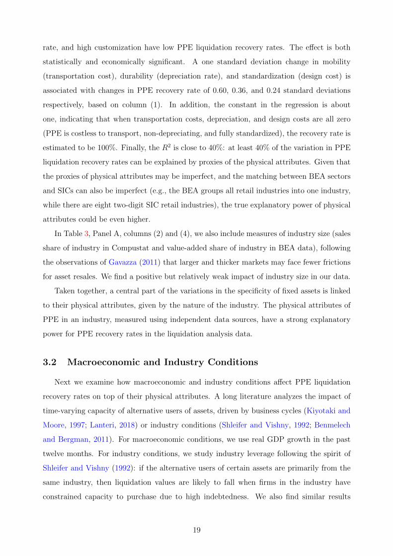
We first verify that disinvestment is less common when asset specificity is higher. For

instance, when PPE has low liquidation values, firms lose more from directly selling it, which

should lead to a lower prevalence of selling PPE on a standalone basis.

For firms in Compustat, we can measure the prevalence of PPE sales using information

from the variable “Sale of Property, Plant, and Equipment” (SPPE), which documents

proceeds from PPE sales. We can measure both the frequency of PPE sales (the fraction of

firm–years with SPPE>0) and the amount of sales (SPPE normalized by lagged net PPE).

Figure 1 plots the average frequency (Panel A) and amount (Panel B) of PPE sales per

year in each two-digit SIC industry on the y-axis, and the industry-average PPE liquidation

22

recovery rate on the x-axis. We see that it is more common to observe PPE sales in industries

with lower PPE specificity (higher recovery rates). Internet Appendix Figure IA5 shows the

corresponding plots using predicted PPE recovery rates based on physical attributes (using

Table 3, Panel A, column (1)), and the patterns are similar. Table 4 shows the relationship

in regressions, using both the raw industry-average PPE recovery rates and PPE recovery

rates predicted by the physical attributes of PPE in each industry (mobility, durability, and

standardization/customization). A one standard deviation increase in industry-average PPE

recovery rate is associated with a roughly 0.32 standard deviation increase in the average

frequency of PPE sales (based on column (1)), and a roughly 0.55 standard deviation increase

in the average amount of PPE sold (based on column (4)).

For industries with high asset specificity, we find that capital reallocation primarily takes

the form of mergers and acquisitions: purchases of firms or segments as a whole (installed

assets together with teams and organizational structures), instead of capital on a standalone

basis. In other words, when assets are specialized, it is important to combine them with

human capital and organizational capital, and assembling human capital and organizational

capital is not frictionless. While such firms can potentially downsize through selling an entire

division or segment, these changes are inevitably lumpier and more drastic. Consequently,

overall firms with more specialized assets would have less flexibility for disinvestment and

face higher investment irreversibility.

Impact of Uncertainty

A key implication of investment irreversibility is that investment is sensitive to uncer-

tainty shocks (see Bloom (2014) for a summary). We test this prediction in Table 5. We

use firm-level uncertainty shocks based on high-frequency stock returns data, similar to the

measure in Gilchrist, Sim, and Zakrajsek (2014). In particular, we study annual regressions:

Yi,t+1 = αi + ηj,t + βσi,t + φλi × σi,t + γXi,t + εi,t, (1)

where σi,t denotes the return volatility of firm i in year t, and λi denotes the liquidation

recovery rate of firm i’s assets based on its industry. The outcome Yi,t+1 is the investment

rate in year t + 1 to allow for lags in investment implementation: investment decisions

may translate into actual investment spending with a delay (Lamont, 2000). The control

variables Xi,t include Q, book leverage cash holdings, EBITDA, size (log book assets), and

ratings at the end of year t, as well as the level of stock returns in year t and its interaction

23

with λ. We include firm fixed effects (αi) and industry-year fixed effects (ηj,t), and double-

cluster standard errors by firm and time. To allow for more variation in uncertainty, we use

a longer sample of 1980 to 2016.

Table 5, Panel A, columns (1) to (4) study capital expenditures (CAPX investment) on

the left hand side, which represent investment in PPE (normalized by lagged net PPE). We

interact PPE liquidation recovery rate (λ) with firm-level return volatility (σ). In columns

(1) and (2), we find that higher uncertainty is associated with significant decreases in capital

expenditures when PPE recovery rates are low, but not when PPE recovery rates are high.

Indeed, when the PPE recovery rate is zero, the coefficient on volatility (β) is significantly

negative; when the PPE recovery rate is one, the coefficient on volatility (β + φ) becomes

roughly zero. In columns (3) and (4), we instrument PPE recovery rates using predicted

values based on physical attributes measured in Section 3.1, and the results are similar.

Table 5, Panel A, columns (5) to (8) study inventory investment, which a large literature

finds to be important for economic fluctuations as well (see Ramey and West (1999) for a

summary). We interact inventory liquidation recovery rate (λ) with firm-level return volatil-

ity (σ). Similarly, we find that higher uncertainty is associated with significant decreases

in inventory investment when inventory recovery rates are low, but not when inventory re-

covery rates are high. The response to uncertainty is again roughly zero if the inventory

recovery rate is one. We can also instrument inventory recovery rate using predicted values

based on the physical attributes of inventory discussed in Internet Appendix Section IA4,

and the results are similar.12

Furthermore, in Table 5, Panel B, we find that the sensitivity of CAPX investment to un-

certainty is affected by PPE recovery rates, but not by inventory recovery rates. Conversely,

the sensitivity of inventory investment to uncertainty is affected by inventory recovery rates,

but not by PPE recovery rates. This clear mapping is supportive of the mechanisms of in-

vestment irreversibility. It shows that the liquidation recovery rates of different types of

assets capture their disinvestment costs (instead of proxying for the severity of financial

frictions the firm faces).

Overall, the empirical findings display a fairly precise correspondence with predictions of

theories on investment irreversibility. They also suggest that the liquidation recovery rates

data performs well both qualitatively and quantitatively.

12Specifically, we use the predicted value from Internet Appendix Table IA7, Panel B, column (1).

24

4.1.2 Pricing Behavior

Woodford (2005) and Altig et al. (2011) point out that when capital is firm-specific

(instead of generic and available from an economy-wide rental market), firms can display

higher price stickiness. As Altig et al. (2011) explain, when a firm considers raising prices,

it understands that a higher price implies less demand and less output; if the capital stock is

costly to adjust, the firm would be left with excess capital, which can decrease its incentive

to increase prices in the first place.

In Table 6, we collect information on industry-level price rigidity using the frequency of

price change data from Nakamura and Steinsson (2008).13 We match and aggregate this

data to two-digit SICs, and study the relationship with industry-level asset specificity. Given

that in practice both PPE and inventory can be relevant for production, we investigate the

connection with the specificity of PPE and inventory. Columns (1) and (2) show that in

industries where asset specificity is lower (i.e., recovery rate is higher, or fraction of firm-

specific PPE as defined in Section 3 is lower), prices appear more flexible. In column

(3) we combine the specificity of different types of assets and compute the firm-level total

liquidation value from PPE and working capital (normalized by book assets) as in Section

2.4. The independent variable is then the industry average of firm-level liquidation value.

Again, we see that in industries where overall firm-level liquidation values are higher (i.e.,

assets more generic), prices are more flexible. Conversely, in industries where overall firm-

level liquidation values are lower (i.e., assets more specific), prices appear stickier. Figure

2 visualizes this relationship by plotting the industry-level frequency of price change on the

y-axis and the industry-average firm liquidation value on the x-axis. Finally, in column (4)

we also “instrument” firm-level total liquidation value using the physical attributes of PPE

(described in Section 3.1) and inventory (described in Internet Appendix Section IA4), and

the results are similar.

In Internet Appendix Tables IA11 and IA12, we also find that firms with a higher degree

of asset specificity have more countercyclical markups, conditional on output gap (log real

GDP minus log potential GDP) and conditional on demand shocks from defense spending

using data from Nekarda and Ramey (2011). While the measurement of markups can be

non-trivial and the mechanisms that affect markup cyclicality can be complicated, this

13In the model of Altig et al. (2011) with Calvo pricing, having firm-specific capital affects the magnitudeof price change. In the data, what is typically measured is instead the frequency of price change. Smallchanges in desired prices in practice may translate to no price change if there are fixed costs of price changeas in menu cost models.

25

stylized fact seems fairly strong.

4.1.3 Productivity Dispersion

Greater investment irreversibility may also imply greater productivity dispersion (Eis-

feldt and Rampini, 2006; Lanteri, 2018), and we show the model prediction in Lanteri (2018)

in Internet Appendix Figure IA6. We present the empirical relationship in our data in Figure

3. The y-axis shows the average annual dispersion in Q within each two-digit SIC industry

(y-axis). The x-axis shows the average firm-level liquidation value of PPE and working

capital (normalized by total book assets) in the industry. We use both regular Q (market

value of assets over book value of assets) in Panel A, and Q accounting for potential impact

of intangibles from Peters and Taylor (2017) in Panel B. We see that industries with lower

liquidation values tend to have higher Q dispersion. Furthermore, this holds for both large

firms (total assets greater than median in Compustat each year) and small firms (total assets

smaller than median). This pattern suggests that the impact of liquidation values is not

necessarily through borrowing constraints, since large firms’ debt capacity is not primar-

ily driven by liquidation value (Lian and Ma, 2020; Kermani and Ma, 2020). Instead, low

liquidation values can work through higher irreversibility of capital investment. Table IA3

presents the corresponding results in regressions, where we also instrument the liquidation

value using the physical attributes of PPE and inventory and find similar results.

4.2 The “New Economy” and Rising Intangibles

In the above, we investigate traditional investment theories, with a focus on fixed assets.

A vibrant recent literature documents that an important trend in the past few decades is

the growing prevalence of intangible assets (Corrado, Hulten, and Sichel, 2009; Peters and

Taylor, 2017; Haskel and Westlake, 2018; Crouzet and Eberly, 2019, 2020), broadly defined

as production assets without physical presence. They include identifiable intangibles such

as computerized information (software, data, recordings, films), usage rights (licenses, ex-

ploration rights, route rights, domain names, etc.), patents and technologies, and brands,

which could be separable and transferable to alternative users on a standalone basis. Intan-

gible assets also include organizational capital, firm-specific human capital, and other forms

of “economic competencies” (Corrado, Hulten, and Sichel, 2005), which are not necessarily

independently identifiable or separable from the firm.

26

How does rising intangibles affect firms’ asset specificity? A major theme in recent

research is the concern that rising intangibles could substantially decrease firms’ liquidation

values (Giglio and Severo, 2012; Caggese and Perez-Orive, 2018; Haskel and Westlake, 2018;

Falato et al., 2020). We analyze this issue in the following. For identifiable intangibles,

many are transferable on a standalone basis (e.g., software, excavation rights, airlines’ gate

and route rights, patents), and our data provides some information about their liquidation

recovery rates. For other intangibles that are integral to the firm (e.g., organizational

capital), they cannot be separated from the firm and have no liquidation value.

We provide several findings relevant for understanding the impact of rising intangibles.

First, building on the discussions above, we further flesh out that physical assets of non-

financial firms are already highly specific and liquidation values are low to begin with.

Second, in many industries, the liquidation recovery rate of identifiable intangibles is not

necessarily much lower than that of PPE, in part because intangibles do not face trans-

portation costs given the absence of physical presence. Third, based on existing measures

of intangible assets, the rise in intangibles is more pronounced in industries where physical

assets are more specific (PPE liquidation recovery rate is lower) in the first place. Taken to-

gether, we find that the impact of rising intangibles on firms’ asset specificity and liquidation

values has been relatively limited so far.

We discuss each of these findings in detail below. First, as shown in Section 2, physical

assets are already quite specific in many industries. For instance, the mean industry-level

liquidation recovery rate for PPE is about 35%. In this case, even if PPE is increasingly

replaced by intangible assets with minimal liquidation recovery rates, the change in the total

liquidation value may not be substantial.

Second, we investigate the liquidation recovery rate of identifiable intangibles. In partic-

ular, our data includes the estimated liquidation recovery rate of book intangibles, which are

intangible assets acquired from external parties and therefore capitalized on balance sheet

based on the current accounting rules in the US. Intangible assets developed internally, on

the other hand, are expensed rather than capitalized under US accounting rules, and do not

show up among book assets. Book intangibles have two components. The first component

mainly represents identifiable intangibles (such as software, customer data, usage rights,

patents, among others), which can be acquired independently from external parties. This

part generally has positive liquidation recovery rates. The second component is goodwill

(i.e., the premium between the total purchase price in an acquisition and the net book value

27

of all identifiable assets, which may come from the value of human capital, organizational

capital, or from over-pricing), and has zero liquidation value almost by definition.

Figure 4 plots the average liquidation recovery rate of PPE versus book intangibles for

Fama-French 12 industries. For each industry, the first bar represents the average PPE

recovery rate; the second bar represents the average book intangible recovery rate; the third

bar represents the implied recovery rate of non-goodwill book intangibles, calculated as the

average book intangible recovery rate divided by one minus the industry-average share of

goodwill in total book intangibles. We see that the second bar, and especially the third bar,

are not much lower than the first bar. For two-digit SIC industries, the mean industry-level

recovery rate of book intangibles is about 18%, with an inter-quartile range from 2% to 25%;

the mean industry-level recovery rate of non-goodwill book intangibles is about 37%, with

an inter-quartile range from 2% to 50%. The level of non-goodwill book intangible recovery

rates is comparable to that of PPE recovery rates, although with more variance.14 In sum,

identifiable intangibles can obtain liquidation values on their own, and may not necessarily

be more specific than tangible assets like PPE.

Third, we find that rising intangibles seem especially pronounced in industries where

physical assets are more specific in the first place. We measure the stock of intangibles in

several ways. One is the BEA’s estimate of the stock of intellectual property for each BEA

industry (relative to BEA’s estimate of the stock of fixed assets in the industry). Another is

Peters and Taylor (2017)’s estimate of the stock of intangibles for Compustat firms (relative

to their net PPE), which includes both book intangibles and the estimated stock of off-

balance sheet intangibles. Peters and Taylor (2017) capitalize R& D spending to estimate

knowledge capital, and capitalize 30% of Selling, General, and Administration expenses

to estimate organizational capital. They then combine these values with book intangibles

to form an estimate of the total stock of intangibles. Although these measures could be

imperfect, the pattern we document is fairly robust to the measurement of intangibles.

Figure 5 plots the change in the industry-level share of intangible assets relative to

the sum of PPE and intangibles from 1996 and 2016 (y-axis) against industry-level PPE

recovery rates (x-axis). We use the BEA’s measurement of intangibles in Panel A, and

14To put the level of intangible recovery rate in perspective, we may need to bear in mind several factors.One is that given the eligibility criteria for book intangibles (i.e., acquired from external parties), they mayselect for intangible assets that are easier to trade and purchase, and select for those with higher liquidationrecovery rates. Another is that the market for trading intellectual properties and other identifiable intangi-bles (various types of rights) is developing over time (Mann, 2018), so intangible recovery rates in the futuremay be enhanced as more markets develop and mature.

28

Peters and Taylor (2017)’s estimate in Panel B. Table 7 shows the results in regressions,

using both direct measurement of PPE recovery rates and PPE recovery rates instrumented

by physical attributes of PPE. In all cases, industries with low PPE recovery rates have

seen the most substantial increase in the relative prevalence of intangibles. In other words,

even if intangibles have lower liquidation values, the shift from physical assets like PPE to

intangibles has been greater where PPE’s recovery rates are already small, and there is not

much to “lose” further.

Finally, putting these observations together, Figure 6 shows the estimated liquidation

value of all Compustat firms, as a share of total book value (Panel A) and as a share of

total enterprise value (Panel B), from 1996 to 2016. Liquidation values include those from

book intangibles, PPE, working capital, and cash. We see that the estimated liquidation

value from PPE declines slightly over this period (by about 2% of book assets), which is

offset by an increase in the liquidation value of book intangibles. Meanwhile, firms have less

receivables and more cash. Overall, total liquidation values do not seem to change drastically,

although by many measures the prevalence of intangibles has increased substantially over

this period (Crouzet and Eberly, 2019). Indeed, the sum of liquidation value from PPE and

book intangibles (the bottom two bars) has stayed roughly constant (and always below 20%

of both book value of assets and firm enterprise value).

Accordingly, based on our data, it does not appear that rising intangibles has led to a

significant drop in firms’ liquidation values. Correspondingly, it is not necessarily the case

that rising intangibles substantially tighten firms’ borrowing constraints as many papers have

feared. Furthermore, in the US, firms’ debt capacity is not necessarily tied to the liquidation

value of particular assets (Kermani and Ma, 2020; Lian and Ma, 2020), especially when

firms have positive earnings. Similarly, the results also suggest that it is not clear whether

irreversibility increases significantly with rising intangibles. A set of identifiable intangibles

such as licenses and usage rights, data and customer lists, certain patents, etc. could be

reasonably sold off and such investment could be partially reversible.

What then is different about intangibles? An interesting hypothesis is that intangibles

can be more “scalable” (Haskel and Westlake, 2018; Crouzet and Eberly, 2019). Given

that intangibles are not bound by physical presence and physical locations, some intangibles

could be used simultaneously at multiple places (e.g., enterprise planning systems, brands,

data). This effect may lead to higher concentration and the prominence of “superstar”

firms (Hsieh and Rossi-Hansberg, 2020; Covarrubias, Gutierrez, and Philippon, 2020). In

29

addition, rising intangibles may also lead to an apparent decline in investment activities

measured using traditional capital expenditures, which is relevant for national accounting

and understanding economic dynamism (Corrado, Hulten, and Sichel, 2005; Crouzet and

Eberly, 2020). These implications of rising intangibles are likely to be more central than

changes in liquidation values.

5 Connections to Model Parameters

Finally, we summarize the connection between our findings and the parameters used in

two common classes of models.

5.1 Models of Investment Irreversibility

Models of investment irreversibility often need to calibrate or estimate the loss from

disinvestment of the capital stock. In particular, this class of models postulate that firms

spend I+ when they invest, and receive λI− when they disinvest, where λ denotes the

fraction of the purchase price of capital that firms can recover from disinvestment (Bloom,

2009; Abel and Eberly, 1996). Bloom (2009) estimates the loss from disinvestment to be

43%, which translates into a liquidation recovery rate λ of 57%. Lanteri (2018) estimates

the equilibrium loss from disinvesting used capital to be around 7% (i.e., λ as high as 93%).

Our data, like Ramey and Shapiro (2001), implies larger losses from disinvesting fixed assets

on a standalone basis. Our data also suggests that this loss can vary substantially across

industries, which may lead to different patterns in industry dynamics.

Overall, our measurement suggests that if capital reallocation takes the form of directly

selling used fixed assets on a standalone basis, the loss can be significant. However, if

reallocation takes the form of mergers and acquisitions, which transfer not just fixed assets

but also human capital and organizational capital, the loss may not be as substantial, but

such adjustments are inevitably much lumpier and are difficult to implement if the firm

simply wants to downsize its capital stock. Accordingly, high asset specificity inevitably

limits firms’ flexibility to disinvest and downsize.

30

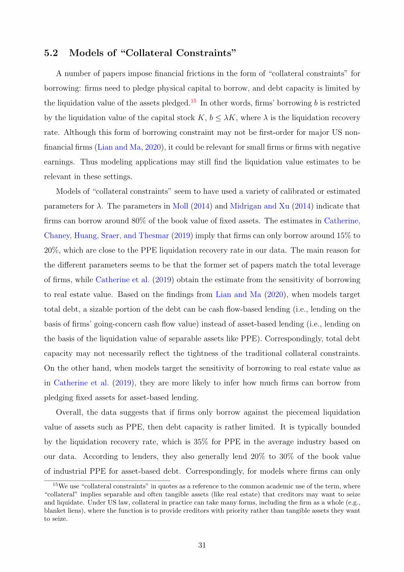
5.2 Models of “Collateral Constraints”

A number of papers impose financial frictions in the form of “collateral constraints” for

borrowing: firms need to pledge physical capital to borrow, and debt capacity is limited by

the liquidation value of the assets pledged.15 In other words, firms’ borrowing b is restricted

by the liquidation value of the capital stock K, b ≤ λK, where λ is the liquidation recovery

rate. Although this form of borrowing constraint may not be first-order for major US non-

financial firms (Lian and Ma, 2020), it could be relevant for small firms or firms with negative

earnings. Thus modeling applications may still find the liquidation value estimates to be

relevant in these settings.

Models of “collateral constraints” seem to have used a variety of calibrated or estimated

parameters for λ. The parameters in Moll (2014) and Midrigan and Xu (2014) indicate that

firms can borrow around 80% of the book value of fixed assets. The estimates in Catherine,

Chaney, Huang, Sraer, and Thesmar (2019) imply that firms can only borrow around 15% to

20%, which are close to the PPE liquidation recovery rate in our data. The main reason for

the different parameters seems to be that the former set of papers match the total leverage

of firms, while Catherine et al. (2019) obtain the estimate from the sensitivity of borrowing

to real estate value. Based on the findings from Lian and Ma (2020), when models target

total debt, a sizable portion of the debt can be cash flow-based lending (i.e., lending on the

basis of firms’ going-concern cash flow value) instead of asset-based lending (i.e., lending on

the basis of the liquidation value of separable assets like PPE). Correspondingly, total debt

capacity may not necessarily reflect the tightness of the traditional collateral constraints.

On the other hand, when models target the sensitivity of borrowing to real estate value as

in Catherine et al. (2019), they are more likely to infer how much firms can borrow from

pledging fixed assets for asset-based lending.

Overall, the data suggests that if firms only borrow against the piecemeal liquidation

value of assets such as PPE, then debt capacity is rather limited. It is typically bounded

by the liquidation recovery rate, which is 35% for PPE in the average industry based on

our data. According to lenders, they also generally lend 20% to 30% of the book value

of industrial PPE for asset-based debt. Correspondingly, for models where firms can only

15We use “collateral constraints” in quotes as a reference to the common academic use of the term, where“collateral” implies separable and often tangible assets (like real estate) that creditors may want to seizeand liquidate. Under US law, collateral in practice can take many forms, including the firm as a whole (e.g.,blanket liens), where the function is to provide creditors with priority rather than tangible assets they wantto seize.

31

borrow against the liquidation value of their fixed assets, the low level of debt capacity

would apply for most industries.

6 Conclusion

Asset specificity is a central issue in many lines of research. Obtaining systematic mea-

sures of the degree of asset specificity across industries has been a long-standing challenge.

We tackle this challenge by constructing a new dataset that measures the liquidation recov-

ery rates of all major asset categories across industries.

We find that non-financial firms’ assets are generally highly specific. For instance, in

the average industry, the liquidation recovery rate of a firm’s plant, property, and equip-

ment (PPE) is about 35%. We also investigate the key determinants of variations in asset

specificity. We find that physical attributes of assets used in different industries have a

strong link with cross-industry variations in asset specificity. We collect a rich set of data

to measure physical attributes such as mobility, durability, and standardization, and show

that they can account for at least around 40% of the variation in industry-average PPE

liquidation recovery rates. We also find that macro and industry conditions affect recovery

rates the most when PPE is not firm-specific. When PPE is customized and firm-specific,

there are few alternative users who want to directly purchase such PPE in any case, and

recovery rates are less responsive to macro or industry conditions.

We then show that the data on asset specificity has broad applications for macro-finance

questions. It aligns closely with firms’ investment behavior, such as the prevalence of dis-

investment and the investment sensitivity to uncertainty shocks, as predicted by classic

theories of investment irreversibility. It also helps understand patterns in price setting and

productivity dispersion, generally in line with model predictions as well. Furthermore, the

data suggests that the first-order impact of rising intangibles may not be to compress firms’

liquidation values. Other implications of rising intangibles, such as the impact on scalabil-

ity, could be more interesting and they may interact with the attributes of physical assets.

Finally, the physical attributes of assets we measure also allow us to establish the links

between asset specificity and macro-finance outcomes based on physical foundations.

Overall, we hope the data is useful for informing key parameters in models, and for

testing and uncovering economic mechanisms.

32

References

Abel, Andrew B, and Janice C Eberly, 1996, Optimal investment with costly reversibility,Review of Economic Studies 63, 581–593.

Almeida, Heitor, and Murillo Campello, 2007, Financial constraints, asset tangibility, andcorporate investment, Review of Financial Studies 20, 1429–1460.

Altig, David, Lawrence J Christiano, Martin Eichenbaum, and Jesper Linde, 2011, Firm-specific capital, nominal rigidities and the business cycle, Review of Economic Dynamics14, 225–247.

Benmelech, Efraim, 2008, Asset salability and debt maturity: Evidence from nineteenth-century american railroads, Review of Financial Studies 22, 1545–1584.

Benmelech, Efraim, and Nittai K Bergman, 2011, Bankruptcy and the collateral channel,Journal of Finance 66, 337–378.

Berger, Philip G, Eli Ofek, and Itzhak Swary, 1996, Investor valuation of the abandonmentoption, Journal of Financial Economics 42, 259–287.

Bernstein, Shai, Emanuele Colonnelli, and Benjamin Iverson, 2019, Asset allocation inbankruptcy, Journal of Finance 74, 5–53.

Bertola, Guiseppe, and Ricardo J Caballero, 1994, Irreversibility and aggregate investment,Review of Economic Studies 61, 223–246.

Bloom, Nicholas, 2009, The impact of uncertainty shocks, Econometrica 77, 623–685.

Bloom, Nicholas, 2014, Fluctuations in uncertainty, Journal of Economic Perspectives 28,153–76.

Bris, Arturo, Ivo Welch, and Ning Zhu, 2006, The costs of bankruptcy: Chapter 7 liquidationversus Chapter 11 reorganization, Journal of Finance 61, 1253–1303.

Caggese, Andrea, and Ander Perez-Orive, 2018, Capital misallocation and secular stagna-tion, Working paper.

Catherine, Sylvain, Thomas Chaney, Zongbo Huang, David Sraer, and David Thesmar,2019, Aggregate effects of collateral constraints, Working paper.

Corrado, Carol, Charles Hulten, and Daniel Sichel, 2005, Measuring capital and technology:An expanded framework, in Measuring capital in the new economy , 11–46 (University ofChicago Press).

Corrado, Carol, Charles Hulten, and Daniel Sichel, 2009, Intangible capital and US economicgrowth, Review of Income and Wealth 55, 661–685.

Covarrubias, Matias, German Gutierrez, and Thomas Philippon, 2020, From good to badconcentration? US industries over the past 30 years, NBER Macroeconomics Annual 34,1–46.

Crouzet, Nicolas, and Janice Eberly, 2020, Rents and intangible capital: A q+ framework,Working paper.

Crouzet, Nicolas, and Janice C Eberly, 2019, Understanding weak capital investment: Therole of market concentration and intangibles, Jackson Hole Symposium.

De Loecker, Jan, Jan Eeckhout, and Gabriel Unger, 2020, The rise of market power and themacroeconomic implications, Quarterly Journal of Economics .

33

Eisfeldt, Andrea L, and Adriano A Rampini, 2006, Capital reallocation and liquidity, Journalof Monetary Economics 53, 369–399.

Falato, Antonio, Dalida Kadyrzhanova, Jae Sim, and Roberto Steri, 2020, Rising intangiblecapital, shrinking debt capacity, and the US corporate savings glut, Working paper.

Flynn, Zach, Amit Gandhi, and James Traina, 2019, Identifying market power in productiondata, Working paper.

Gavazza, Alessandro, 2011, The role of trading frictions in real asset markets, AmericanEconomic Review 101, 1106–43.

Giglio, Stefano, and Tiago Severo, 2012, Intangible capital, relative asset shortages andbubbles, Journal of Monetary Economics 59, 303–317.

Gilchrist, Simon, Raphael Schoenle, Jae Sim, and Egon Zakrajsek, 2017, Inflation dynamicsduring the financial crisis, American Economic Review 107, 785–823.

Gilchrist, Simon, Jae W Sim, and Egon Zakrajsek, 2014, Uncertainty, financial frictions,and investment dynamics, Working paper.

Gulen, Huseyin, and Mihai Ion, 2016, Policy uncertainty and corporate investment, Reviewof Financial Studies 29, 523–564.

Haskel, Jonathan, and Stian Westlake, 2018, Capitalism without capital: The rise of theintangible economy (Princeton University Press).

Hsieh, Chang-Tai, and Esteban Rossi-Hansberg, 2020, The industrial revolution in services,Working paper.

Kermani, Amir, and Yueran Ma, 2020, Two tales of debt, Working paper.

Kim, Hyunseob, and Howard Kung, 2017, The asset redeployability channel: How uncer-tainty affects corporate investment, Review of Financial Studies 30, 245–280.

Kiyotaki, Nobuhiro, and John Moore, 1997, Credit cycles, Journal of Political Economy105.

Lamont, Owen A, 2000, Investment plans and stock returns, Journal of Finance 55, 2719–2745.

Lanteri, Andrea, 2018, The market for used capital: Endogenous irreversibility and reallo-cation over the business cycle, American Economic Review 108, 2383–2419.

Lian, Chen, and Yueran Ma, 2020, Anatomy of corporate borrowing constraints, Workingpaper.

Maksimovic, Vojislav, and Gordon Phillips, 2001, The market for corporate assets: Whoengages in mergers and asset sales and are there efficiency gains?, Journal of Finance 56,2019–2065.

Mann, William, 2018, Creditor rights and innovation: Evidence from patent collateral,Journal of Financial Economics 130, 25–47.

Midrigan, Virgiliu, and Daniel Yi Xu, 2014, Finance and misallocation: Evidence fromplant-level data, American Economic Review 104, 422–58.

Moll, Benjamin, 2014, Productivity losses from financial frictions: Can self-financing undocapital misallocation?, American Economic Review 104, 3186–3221.

Murfin, Justin, and Ryan Pratt, 2019, Who finances durable goods and why it matters:Captive finance and the coase conjecture, Journal of Finance 74, 755–793.

34

Nakamura, Emi, and Jon Steinsson, 2008, Five facts about prices: A reevaluation of menucost models, Quarterly Journal of Economics 123, 1415–1464.

Nekarda, Christopher J, and Valerie A Ramey, 2011, Industry evidence on the effects ofgovernment spending, American Economic Journal: Macroeconomics 3, 36–59.

Nunn, Nathan, 2007, Relationship-specificity, incomplete contracts, and the pattern of trade,Quarterly Journal of Economics 122, 569–600.

Ottonello, Pablo, 2018, Capital unemployment, Working paper.

Peters, Ryan H, and Lucian A Taylor, 2017, Intangible capital and the investment-q relation,Journal of Financial Economics 123, 251–272.

Pindyck, Robert S, 1991, Irreversibility, uncertainty, and investment, Journal of EconomicLiterature 29, 1110.

Ramey, Valerie A, and Matthew D Shapiro, 2001, Displaced capital: A study of aerospaceplant closings, Journal of Political Economy 109, 958–992.

Ramey, Valerie A, and Kenneth D West, 1999, Inventories, Handbook of Macroeconomics 1,863–923.

Rauch, James E, 1999, Networks versus markets in international trade, Journal of Interna-tional Economics 48, 7–35.

Shleifer, Andrei, and Robert W Vishny, 1992, Liquidation values and debt capacity: Amarket equilibrium approach, Journal of Finance 47, 1343–1366.

Traina, James, 2018, Is aggregate market power increasing? Production trends using finan-cial statements, Working paper.

Williamson, Oliver E, 1981, The economics of organization: The transaction cost approach,American Journal of Sociology 87, 548–577.

Woodford, Michael, 2005, Firm-specific capital and the New Keynesian Phillips Curve,International Journal of Central Banking .

35

Main Figures and Tables

Figure 1: PPE Liquidation Recovery Rates and Prevalence of PPE Sales

The x-axis is the industry-average PPE liquidation recovery rate. The y-axis is the industry-average fre-quency of having non-zero PPE sales in Panel A, and the industry-average PPE sale value (normalized bylagged net PPE) in Panel B. Sample period is 1996 to 2016. Each industry is a two-digit SIC.

Panel A. Frequency of PPE Sales

0.2

.4.6

.81

Annu

al %

Firm

s Se

lling

PPE

0 20 40 60 80 100PPE Liquidation Recovery Rate

Panel B. PPE Sold/Net Book PPE

0.0

5.1

.15

Sale

of P

PE/T

otal

PPE

0 20 40 60 80 100PPE Liquidation Recovery Rate

36

Figure 2: Asset Specificity and Frequency of Price Change

The x-axis is the industry-average firm liquidation value (including PPE and working capital, normalizedby total book assets) as constructed in Section 2.4. The y-axis is the industry-level frequency of pricechange, based on data from Nakamura and Steinsson (2008) (% price change per month). Each industry isa two-digit SIC.

020

4060

80Pr

ice

Cha

nge

Freq

uenc

y in

Indu

stry

.1 .2 .3 .4Average Firm Liquidation Value in Industry

37

Figure 3: Asset Specificity and Dispersion of Q

This figure shows binscatter plots of industry-level dispersion in Q. We calculate cross-sectional standarddeviation of Q for each two-digit SIC industry and each year. The x-axis is the industry-average firmliquidation value (including PPE and working capital, normalized by total book assets) constructed inSection 2.4. The y-axis is the average annual standard deviation in Q. In Panel A, Q is market value ofassets (book assets minus book equity plus market value of equity) divided by book value of assets. In PanelB, Q is the estimate adjusted for intangibles from Peters and Taylor (2017). We calculate Q dispersion forlarge firms (assets above Compustat median in each year) and small firms (assets below Compustat median),and show binscatter plots for each group. Sample period is 1996 to 2016.

Panel A. Standard Average Q

.51

1.5

2St

anda

rd D

evia

tion

of Q

.1 .2 .3 .4Average Firm Liquidation Value in Industry

Large Firms Small Firms

Panel B. Q Adjusted for Intangibles (Peters and Taylor, 2017)

.51

1.5

22.

5St

anda

rd D

evia

tion

of Q

.1 .2 .3 .4Average Firm Liquidation Value in Industry

Large Firms Small Firms

38

Figure 4: Industry-Average Recovery Rate: PPE vs. Book Intangibles

This figure shows the average recovery rate of PPE versus book intangibles in each Fama-French 12 industry(except financials). For each industry, the first bar shows the mean PPE recovery rate. The second barshows the mean book intangible recovery rate. The third bar shows the estimated book intangible recoveryrate excluding goodwill, which is calculated as the mean book intangible recovery rate divided by one minusthe share of goodwill in book intangibles in the industry. In other words, we assume (as is generally thecase) that the liquidation recovery rate of goodwill is zero. Then all the liquidation value of book intangiblescomes from non-goodwill assets.

020406080

100

020406080

100

020406080

100

Consumer NonDurables Consumer Durables Manufacturing Energy

Chemicals Business Equipment Telecommunications Utilities

Wholesale/Retail Healthcare Others

PPEBook IntangibleBook Intangibles (ex. Goodwill)

Mea

n Li

quid

atio

n R

ecov

ery

Rat

e

39

Figure 5: PPE Specificity and Rising Intangibles

Binscatter plots of rising intangibles for different levels of PPE recovery rate. Panel A uses BEA’s estimatesof intellectual property assets in each BEA sector, and the y-axis is the change in intellectual property as ashare of intellectual property plus fixed assets from 1996 to 2016. The x-axis is the estimated average PPErecovery rate in each BEA sector. Panel B uses Peters and Taylor (2017)’s estimate of total capitalizedintangibles (including book intangibles, capitalized R&D, and capitalized value of 30% of Selling, General,and Administrative Expenses for each Compustat firm. The y-axis is the firm-level change in the capitalizedintangibles as a share of capitalized intangibles plus net PPE from 1996 to 2016. The x-axis is the PPErecovery rate of the firm based on its industry.

Panel A. Sector-Level Intellectual Property Assets (BEA)

-.2-.1

0.1

.2IP

Sha

re: 2

006

min

us 1

996

0 .2 .4 .6 .8 1PPE Recovery Rate

Panel B. Firm-Level Intangibles (Compustat)

0.0

5.1

.15

.2In

tang

ible

Sha

re: 2

016

min

us 1

996

.1 .2 .3 .4 .5PPE Recovery Rate

40

Figure 6: Estimated Firm-Level Liquidation Value and Composition Over Time(Compustat Aggregate)

This figure shows the estimated total liquidation value from PPE, working capital, book intangibles, andcash of all Compustat firms from 1996 to 2016. Panel A shows total liquidation value as a share of totalbook assets. Panel B shows total liquidation value as a share of total enterprise value.

Panel A. Total Liquidation Value over Total Book Assets

0

.2

.4

.6

.8

1

1996 2006 2016

Book Intangible PPEInventory ReceivableCash

Panel B. Total Liquidation Value over Total Enterprise Value

0

.2

.4

.6

.8

1

1996 2006 2016

Book Intangible PPEInventory ReceivableCash

41

Table 1: Summary of Industry-Average Recovery Rates

This table presents summaries of industry-average recovery rates. Each industry is a two-digit SIC code.

Panel A. Plant, Property, and Equipment (PPE)

Mean: 0.35; 75th: 0.44; 25th: 0.24High: Transportation (0.69), Lumber (0.58), Wholesale (0.57)Low: Personal services (0.08), Educational services (0.15)

Panel B. Inventory

Mean: 0.44; 75th: 0.56; 25th: 0.34High: Auto dealers (0.88), Apparel stores (0.75), Supermarkets (0.75)Low: Restaurants (0.15), Special construction (0.2), Communications (0.26)

Panel C. Receivable

Mean: 0.63; 75th: 0.71; 25th: 0.55High: Utilities (0.90), Medical/optical devices (0.89), Coal (0.79)Low: Airlines (0.37), Educational services (0.37)

42

Table 2: Summary Statistics of Compustat Firms

Panel A shows the statistics of firm-level liquidation value estimates, which combine the book value ofassets with liquidation recovery rates based on the firm’s industry (two-digit SIC). Liquidation values arenormalized by total book assets. Panel B shows other basic statistics. The sample covers annual data from1996 to 2016.

Panel A. Liquidation Value Statistics

Variable mean p25 p50 p75 s.d. N

Liquidation value: PPE, inventory, receivable 0.23 0.12 0.23 0.33 0.13 107,378Liquidation value: PPE, inventory, receivable, cash 0.44 0.30 0.41 0.54 0.20 106,482Liquidation value: PPE 0.09 0.02 0.05 0.12 0.09 110,222Liquidation value: inventory 0.05 0.00 0.02 0.07 0.07 110,523Liquidation value: receivable 0.09 0.03 0.07 0.13 0.09 112,031Cash/assets 0.21 0.02 0.10 0.31 0.25 117,588

Panel B. Other Statistics

Variable mean p25 p50 p75 s.d. N

Log assets 4.80 3.08 4.94 6.76 2.83 118,594Log market cap 5.58 4.02 5.54 7.03 2.14 81,687EBITDA 278.91 -1.12 9.39 102.53 1592.02 118,305EBITDA/l.assets -0.19 -0.06 0.09 0.17 1.49 108,705Debt/assets 0.35 0.02 0.21 0.41 0.77 116,929Q 2.05 1.10 1.49 2.32 1.67 79,937MTB 2.92 1.12 1.96 3.53 3.88 79,824PPE/assets 0.25 0.06 0.17 0.39 0.24 115,734Inventory/assets 0.10 0.00 0.04 0.17 0.13 116,212Receivable/assets 0.15 0.04 0.11 0.21 0.14 117,754

43

Table 3: Determinants of PPE Recovery Rates

This table examines the determinants of PPE recovery rates. Panel A studies the relationship between thephysical attributes of assets in each industry and industry-average PPE recovery rate. Transportation cost(in total production cost of PPE) measures mobility. Depreciation rate measures durability. Design costshare (in total production cost of PPE) measures standardization/customization. Sales share of an industryin Compustat and value added share of an industry in BEA data capture industry size. All attributes aremeasured using BEA input-output table or Compustat data in 1997. Columns (1) and (2) use two-digitSICs; columns (3) and (4) use BEA sectors. Panel B studies the relationship between macroeconomic andindustry conditions and firm-level recovery rate within each industry. Past 12-month GDP growth andindustry leverage are measured as of the quarter of the liquidation analysis. In columns (2) and (4), weinteract GDP growth and industry leverage with the fraction of fixed assets in the industry that are notfirm-specific (the top tercile of the 71 types of fixed assets in BEA fixed asset table by design costs aredesignated as firm-specific). Controls include interactions of transportation cost and depreciation rate withGDP growth (column (2)) and industry leverage (column (4)). Industry fixed effects (two-digit SICs) areincluded. R2 does not include industry fixed effects.

Panel A. Physical Attributes and Industry-Average Recovery Rates

Industry-level PPE Recovery RateIndustry Classification

Two-digit SICs BEA sectors

Transportation cost -0.49*** -0.50*** -0.48*** -0.56***(0.12) (0.12) (0.12) (0.13)

Depreciation rate -0.57*** -0.58*** -1.62** -1.83**(0.19) (0.19) (0.73) (0.76)

Design cost share -1.56* -1.71** -2.47** -2.49**(0.81) (0.84) (0.95) (0.94)

Industry size (sales share) 0.39(0.58)

Industry size (value-added share) 1.48(1.12)

Constant 1.00*** 1.02*** 1.13*** 1.16***(0.21) (0.21) (0.19) (0.19)

Obs 48 48 45 45R2 0.40 0.40 0.29 0.33

Robust standard errors in parentheses

Panel B. Impact of Time-Varying Macroeconomic and Industry Conditions

Case-level PPE Recovery Rate(1) (2) (3) (4)

GDP growth 0.37 -6.86(0.69) (4.28)

GDP growth × fraction PPE not firm-specific 12.13*(5.98)

Industry leverage -0.46*** 0.05(0.14) (1.65)

Industry leverage × fraction PPE not firm-specific -3.07*(1.59)

Fixed effect IndustryControls N Y N Y

Obs 349 349 349 349R2 0.001 0.018 0.011 0.020

Standard errors in parentheses, double-clustered by industry and time

44

Table 4: PPE Liquidation Recovery Rate and Prevalence of PPE Sales

The left-hand-side variable is the average fraction of firms with non-zero PPE sales every year in columns(1) and (2), and average PPE sale proceeds (Compustat SPPE) normalized by lagged net PPE (CompustatPPENT) in columns (3) and (4). The right-hand-side is raw industry-average PPE liquidation recovery rateswhen “IV” is labeled “N,” and PPE recovery rates predicted by physical attributes (mobility, durability,standardization/customization shown in Table 3, Panel A, column (1)) when “IV” is labeled “Y.”

Frequency of PPE Sales PPE Sold/Net Book PPE(1) (2) (3) (4)

PPE recovery rate 0.330** 0.887*** 0.061* 0.079***(0.133) (0.289) (0.033) (0.028)

Constant 0.362*** 0.165* -0.001 -0.008(0.060) (0.099) (0.011) (0.009)

IV N Y N Y

Obs 48 48 48 48R2 0.10 0.30

Robust standard errors in parentheses

45

Table 5: Asset Specificity and Investment Response to Uncertainty

Firm-level annual regressions: Yi,t+1 = αi+ηj,t+βσi,t+φλi×σi,t+γXi,t+εi,t. In Panel A columns (1) to (4), Yi,t+1

is capital expenditures (normalized by lagged net PPE), and λi is the PPE recovery rate based on firm i’s industry.In columns (5) to (8), Yi,t+1 is inventory investment (changes in total inventory, normalized by lagged inventory),and λi is the inventory recovery rate based on firm i’s industry. In columns (3) and (4), the PPE recovery rateis instrumented by the predicted recovery rate based on PPE physical attributes discussed in Section 3.1 (“IV”labeled “Y”). In columns (7) and (8), the inventory recovery rate is instrumented by the predicted recovery ratebased on inventory physical attributes discussed in Internet Appendix Section IA4 (“IV” labeled “Y”). σi,t isfirm-level annual stock return volatility in columns (1), (3), (5) and (7), and annual abnormal volatility (based onthe Fama-French three-factor model) in columns (2), (4), (6), and (8). In Panel B, the variables are the same asthose in Panel A columns (1), (2), (5), and (6). The controls Xi,t include Q (market value of assets/book valueof assets), book leverage, cash holdings, EBITDA (normalized by lagged book assets), and size (log book assets)at the end of year t, as well as the level of stock returns in year t and its interaction with λ. Firm, industry-year,and ratings fixed effects are included. R2 does not include fixed effects. Standard errors are double-clustered byfirm and time. The sample period is 1980 to 2016.

Panel A. Baseline Results

CAPX Invest Rate Inventory Invest Rate(1) (2) (3) (4) (5) (6) (7) (8)

Vol -3.00*** -5.03*** -4.24*** -4.40***(0.40) (0.80) (0.56) (0.94)

Vol × PPE recovery rate 2.88** 9.04***(1.06) (2.26)

Vol × Invt recovery rate 3.96*** 4.38*(1.24) (2.20)

Abnormal vol (3-fac) -3.17*** -5.60*** -4.47*** -5.51***(0.40) (0.86) (0.55) (1.14)

Abnormal vol (3-fac) × PPE recovery rate 2.83** 10.17***(1.09) (2.43)

Abnormal vol (3-fac) × Invt recovery rate 4.07*** 6.57**(1.27) (2.80)

IV N N Y Y N N Y YFixed effect Firm. Industry-Year. Rating.

Obs 113,319 113,319 113,319 113,319 95,764 95,764 94,722 94,722R2 0.09 0.09 0.06 0.06

Standard errors in parentheses, clustered by firm and time

Panel B. Additional Results

CAPX Invest Rate Inventory Invest Rate(1) (2) (3) (4)

Vol -3.64*** -3.86***(0.46) (0.82)

Vol × PPE recovery rate 2.65** -1.26(1.08) (1.66)

Vol × Invt recovery rate 1.76* 4.06***(0.89) (1.22)

Abnormal vol (3-fac) -3.80*** -4.10***(0.46) (0.82)

Abnormal vol (3-fac) × PPE recovery rate 2.59** -1.23(1.11) (1.69)

Abnormal vol (3-fac) × Invt recovery rate 1.73* 4.16***(0.87) (1.24)

Fixed effect Firm. Industry-Year. Rating.

Obs 113,319 113,319 95,764 95,764R2 0.09 0.09 0.06 0.06

Standard errors in parentheses, clustered by firm and time

46

Table 6: Asset Specificity and Price Rigidity

The left-hand-side variable is the industry-level frequency of price change, based on data from Nakamuraand Steinsson (2008) (% price change per month). The right-hand-side variables include PPE recoveryrates, inventory recovery rates, the fraction of PPE firm-specific following the categorization in Section3.2, and industry-average firm liquidation values (including PPE and working capital, normalized by totalbook assets) as constructed in Section 2.4. In column (4), the industry-average firm liquidation value isinstrumented using the predicted PPE recovery rate based on physical attributes of PPE (see Section 3.1)and the predicted inventory recovery rate based on physical attributes of inventory (see Internet AppendixSection IA4). Each industry is a two-digit SIC.

Frequency of Price Change in Industry(1) (2) (3) (4)

PPE recovery rate 8.43(18.21)

Frac of PPE firm-specific -19.51*(10.49)

Inventory recovery rate 38.52*** 39.57***(10.71) (9.27)

Ind avg firm liq val 85.68*** 57.29**(22.83) (26.98)

Constant 1.53 9.76* -1.22 6.38(5.24) (5.92) (4.86) (7.39)

IV N N N Y

Obs 44 44 44 42R2 0.16 0.19 0.22

Robust standard errors in parentheses

47

Table 7: PPE Specificity and Rising Intangibles

This table shows the relationship between PPE specificity and rising intangibles. Panel A measures intan-gibles using BEA’s estimates of intellectual property assets in each BEA sector. The left-hand-side variableis IP asset stock as a share of fixed asset plus IP asset. Panel B uses Peters and Taylor (2017)’s estimateof total capitalized intangibles (including book intangibles, capitalized R&D, and capitalized value of 30%of Selling, General, and Administrative Expenses for each Compustat firm. The left-hand-side variable isintangible stock as a share of intangibles and net PPE. Columns (1) and (2) show the relationship betweenintangibles in 1996 and PPE specificity. Columns (3) and (4) show the relationship between intangible sharechange between 1996 and 2016 and PPE specificity. Columns (2) and (4) instrument PPE recovery ratesusing predicted values based on PPE physical attributes (“IV” labeled “Y”).

Panel A. Sector-Level Intellectual Property Assets (BEA)

IP/(IP+Fixed Asset)1996 2016 minus 1996

(1) (2) (3) (4)

PPE recovery rate -0.163** -0.523** -0.081** -0.177**(0.079) (0.221) (0.033) (0.076)

Constant 0.178*** 0.303*** 0.055*** 0.088***(0.045) (0.093) (0.016) (0.030)

IV N Y N Y

Obs 45 45 45 45R2 0.03 0.08

Standard errors in parentheses

Panel B. Firm-Level Intangibles (Compustat)

Intangibles/(Intangibles+PPE)1996 2016 minus 1996

(1) (2) (3) (4)

PPE recovery rate -0.442 -0.675 -0.249*** -0.501***(0.383) (0.541) (0.095) (0.159)

Constant 0.762*** 0.839*** 0.197*** 0.280***(0.117) (0.189) (0.034) (0.056)

IV N Y N Y

Obs 6,964 6,964 1,509 1,509R2 0.02 0.01

Standard errors in parentheses, clustered by industry

48

Internet Appendix

IA1 Additional Figures and Tables

Figure IA1: Liquidation Analysis Reporting Examples

This figure shows examples of summary tables in liquidation analysis in Chapter 11. Panel A comes fromLyondell Chemical (case number 09-10023). Panel B comes from Sorensen Communications (case number14-10454).

Panel A. Lyondell Chemical

Panel B. Sorenson Communications

49

Figure IA2: PPE Liquidation Recovery Rates and PPE Sale Recovery Rates (Compustat)

The x-axis is the industry-average liquidation recovery rate of PPE from liquidation analysis in Chapter 11filings. The y-axis is the industry-average sale recovery rate of PPE computed among Compustat firms. Webegin with firm-years with positive PPE sale proceeds (Compustat variable SPPE). We compute the netbook value of PPE sold based on lagged net book value of PPE plus capital expenditures minus depreciationminus current net book value of PPE. We exclude firm-years with positive acquisition spending, where it isdifficult to tease out the change in PPE book value due to acquisitions. We compute the PPE sale recoveryrate as PPE sale proceeds divided by the net book value of PPE sold. We winsorize this variable at onepercent and take average in each two-digit SIC industry (from 2000 to 2016, same as the time period forthe liquidation recovery rate data), which produces the industry-level PPE sale recovery rate.

0.2

.4.6

.8PP

E Sa

le R

ecov

ery

Rat

e

0 .2 .4 .6 .8 1PPE Liquidation Recovery Rate

50

Figure IA3: Firm-Level Liquidation Value Estimates: Distribution and Composition

Panel A shows the distribution of estimated firm-level liquidation value, including PPE, inventory, andreceivable, normalized by total book assets. Panel B shows the composition for the average firm. Thesample period covers 1996 to 2016.

Panel A. Firm-Level Liquidation Value (PPE, Inventory, Receivable)

0.5

11.

52

2.5

Den

sity

0 .2 .4 .6 .8Liquidation Value/Book Assets

Panel B. Composition of Liquidation Value for Average Firm

9.3%

4.7%

8.5%

Cash Receivables InventoryPPE Unaccounted

51

Figure IA4: PPE Recovery Rates and Industry Conditions

This figure shows binscatter plots of PPE recovery rates for each case (y-axis) and industry conditionsmeasured based on the average book leverage in the industry of Compustat firms. The solid red dotsrepresent observations from industries where the average PPE recovery rate is in the top tercile (industrieswith the most general PPE). The hollow blue dots represent observations from industries where the averagePPE recovery rate is in the bottom tercile (industries with the most specific PPE).

0.1

.2.3

.4.5

.6PP

E R

ecov

ery

Rat

e

.2 .25 .3 .35 .4 .45 .5Industry Leverage

Top Tercile Bottom Tercile

52

Figure IA5: PPE Liquidation Recovery Rate and Prevalence of PPE Sales

The x-axis is the industry-average PPE liquidation recovery rate, predicted based on physical attributes (asin Table 3, Panel A, column (1)). The y-axis is industry-average frequency of having non-zero PPE salesin Panel A, and industry-average PPE sale value (normalized by lagged net PPE) in Panel B. The sampleperiod is 1996 to 2016.

Panel A. Frequency of PPE Sales0

.2.4

.6.8

1An

nual

% F

irms

Sellin

g PP

E

0 20 40 60Predicted PPE Liquidation Recovery Rate

Panel B. PPE Sold/Net Book PPE

0.0

5.1

.15

Sale

of P

PE/T

otal

PPE

0 20 40 60Predicted PPE Liquidation Recovery Rate

53

Figure IA6: Investment Irreversibility and Productivity Dispersion

This figure shows the relationship between MRK dispersion (y-axis) and the parameter of investment irre-versibility ε in the model of Lanteri (2018) (x-axis). Lower ε means higher investment irreversibility. z isthe productivity parameter, and we use two values of z as in Figure 5 of Lanteri (2018).

54

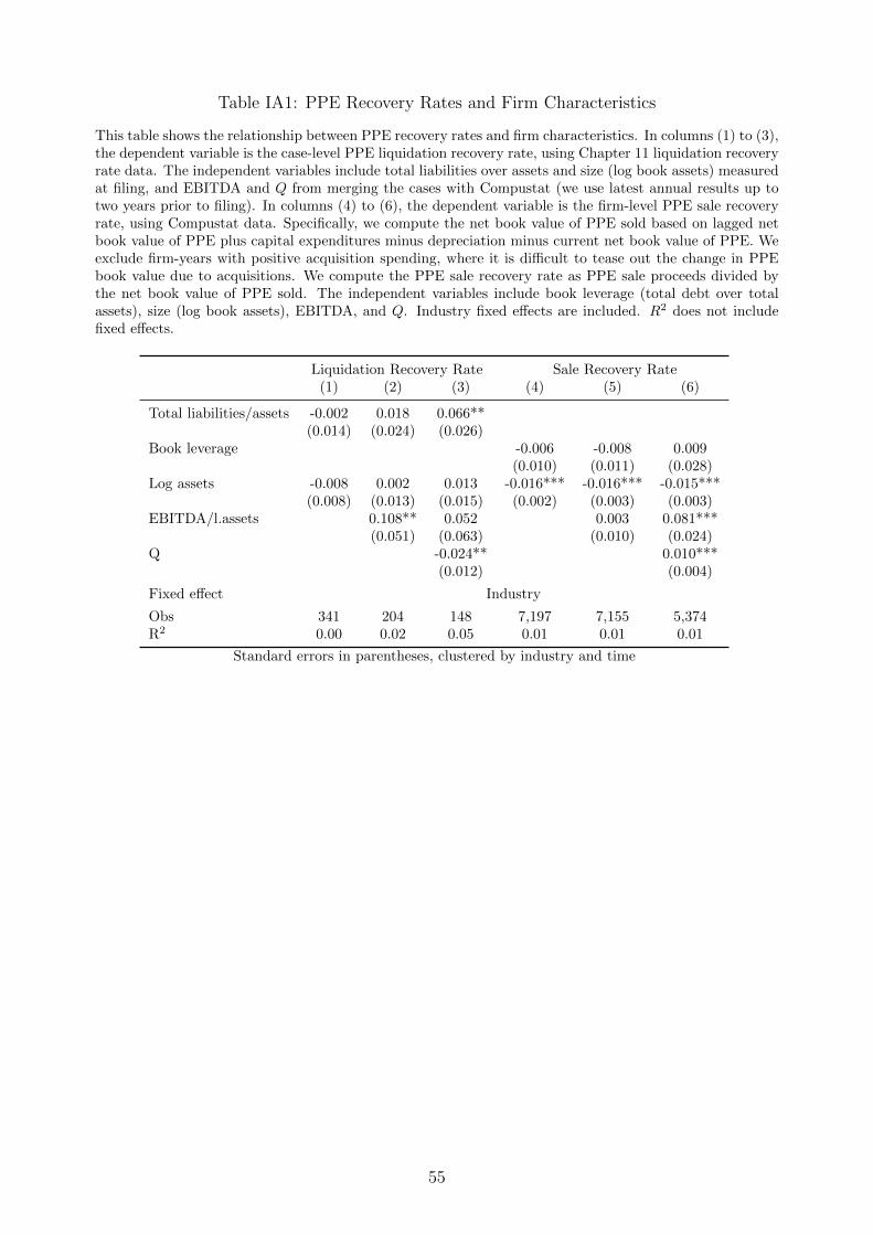
Table IA1: PPE Recovery Rates and Firm Characteristics

This table shows the relationship between PPE recovery rates and firm characteristics. In columns (1) to (3),the dependent variable is the case-level PPE liquidation recovery rate, using Chapter 11 liquidation recoveryrate data. The independent variables include total liabilities over assets and size (log book assets) measuredat filing, and EBITDA and Q from merging the cases with Compustat (we use latest annual results up totwo years prior to filing). In columns (4) to (6), the dependent variable is the firm-level PPE sale recoveryrate, using Compustat data. Specifically, we compute the net book value of PPE sold based on lagged netbook value of PPE plus capital expenditures minus depreciation minus current net book value of PPE. Weexclude firm-years with positive acquisition spending, where it is difficult to tease out the change in PPEbook value due to acquisitions. We compute the PPE sale recovery rate as PPE sale proceeds divided bythe net book value of PPE sold. The independent variables include book leverage (total debt over totalassets), size (log book assets), EBITDA, and Q. Industry fixed effects are included. R2 does not includefixed effects.

Liquidation Recovery Rate Sale Recovery Rate(1) (2) (3) (4) (5) (6)

Total liabilities/assets -0.002 0.018 0.066**(0.014) (0.024) (0.026)

Book leverage -0.006 -0.008 0.009(0.010) (0.011) (0.028)

Log assets -0.008 0.002 0.013 -0.016*** -0.016*** -0.015***(0.008) (0.013) (0.015) (0.002) (0.003) (0.003)

EBITDA/l.assets 0.108** 0.052 0.003 0.081***(0.051) (0.063) (0.010) (0.024)

Q -0.024** 0.010***(0.012) (0.004)

Fixed effect Industry

Obs 341 204 148 7,197 7,155 5,374R2 0.00 0.02 0.05 0.01 0.01 0.01

Standard errors in parentheses, clustered by industry and time

55

Table IA2: Equipment Auction Values and Macroeconomic Conditions

This table uses equipment auction values analyzed by Murfin and Pratt (2019), and studies the impactof macroeconomic conditions (measured using past 12-month real GDP growth). In columns (1) and (2),we control for fixed effects of manufacturer-type, age-type, quarter (seasonality)-type, and condition. Incolumns (3) and (4), we use very restrict fixed effects of manufacturer-type-age-condition and quarter-type.We use nominal equipment auction values in columns (1) and (3), and control for inflation of general purposemachinery and equipment. We use real equipment values in columns (2) and (4), which deflate the nominalauction values by the price index for general purpose machinery and equipment. We also control for a linearannual time trend. Sample period is 1994 and 2013, with nearly one million equipment auctions. R2 doesnot include the fixed effects. Standard errors are clustered by manufacturer-type and year. We are gratefulto Justin Murfin for generously helping with the analysis.

Log Auction ValueNominal Real Nominal Real

(1) (2) (3) (4)

GDP growth 3.14*** 2.95*** 3.20*** 2.99***(0.350) (0.523) (0.347) (0.507)

Inflation 3.75*** 3.79***(0.634) (0.635)

Time trend 0.02*** -0.00 0.02*** -0.00(0.003) (0.003) (0.003) (0.003)

Fixed effect Manufacturer×Type, Age×Type, Manufacturer×Type×Age×Condition,Quarter×Type, Condition Quarter×Type

Observations 778,545 778,545 758,415 758,415R2 0.034 0.012 0.038 0.012

Standard errors in parentheses, clustered by manufacturer-equipment type and year

56

Table IA3: Q Dispersion

Industry-level annual regression, where the left-hand-side variable is annual cross-sectional dispersion in Qfor each two-digit SIC industry. Q is market value of assets (book value of assets minus book equity plusmarket value of equity) over book value of assets in columns (1) and (2), and Q adjusted for intangibles fromPeters and Taylor (2017) in columns (3) and (4). Industry-average liquidation value is the annual averagefirm-level liquidation value (including PPE and working capital) constructed in Section 2.4. In columns (2)and (4), industry-average liquidation value is instrumented by PPE and inventory recovery rates predictedbased on their physical attributes (see Section 3.1 and Internet Appendix Section IA4 respectively). Sampleperiod is 1996 to 2016. Year fixed effects are included. R2 does not include fixed effects.

Standard Q Adjusted Q(1) (2) (3) (4)

Ind avg firm liq val -2.05*** -1.99** -3.50*** -2.91*(0.55) (0.77) (1.21) (1.51)

IV N Y N YFixed effect Year

Obs 979 945 981 945R2 0.12 0.10

Standard errors in parentheses, clustered by industry and time

57

IA2 Liquidation Analysis Examples

In the following, we include excerpts of the detailed discussion for the summary liqui-

dation value estimates shown in the example of Lyondell Chemical in Figure IA1. They

explain the procedures for the estimates for PPE, inventory, account receivable, and cash.

Figure IA7: Lyondell Chemical Example: Facility-Level Information for All PPE

This figure shows an excerpt of the discussion about PPE liquidation value estimates in the liquidationanalysis of Lyondell (Panel A) and excerpt of the facility-level estimate in the accompanying appendix.

Panel A. Excerpt of PPE Discussion in Liquidation Analysis

Panel B. Excerpt of Facility-Level Estimate in Liquidation Analysis Appendix

58

Lyondell Chemical Example: Facility-Level Information for All PPE (Cont.)

59

Figure IA8: Lyondell Chemical Example: Other Assets

This figure shows an excerpt of the discussion about inventory, receivable, and cash liquidation value esti-mates in the liquidation analysis of Lyondell.

Panel A. Excerpt of Inventory Discussion in Liquidation Analysis

Panel B. Excerpt of Cash and Receivable Discussion in Liquidation Analysis

60

IA3 Measuring Physical Attributes of PPE

Below we further explain the measurement of the physical attributes of plant, property,

and equipment (PPE). As described in Section 3.1, we utilize information from BEA’s fixed

asset table and input-output table. First, we study which types of assets each industry uses.

We collect information from BEA’s fixed asset table, which shows the stock amount of 71

types of fixed assets in 58 sectors each year. Second, we measure the attributes of each of

the 71 types of assets, which rely on information from BEA’s input-output table. Finally,

we construct the overall industry-level attributes based on the share of each asset in an

industry’s fixed asset stock. The 71 types of fixed assets are listed in Table IA4 below.

Table IA4: List of Assets in BEA Fixed Asset Table

This table shows the 71 types of assets in the BEA Fixed Asset Table. BEA provides the stock amount (netof depreciation) for each of 58 sectors in each year.

Code NIPA Asset Types Code NIPA Asset Types

EQUIPMENT STRUCTURES1 EP1A Mainframes 40 SOO1 Office2 EP1B PCs 41 SB31 Hospitals3 EP1C DASDs 42 SB32 Special care4 EP1D Printers 43 SOO2 Medical buildings5 EP1E Terminals 44 SC03 Multimerchandise shopping6 EP1F Tape drives 45 SC04 Food and beverage establishments7 EP1G Storage devices 46 SC01 Warehouses8 EP1H System integrators 47 SOMO Mobile structures9 EP20 Communications 48 SC02 Other commercial10 EP34 Nonelectro medical instruments 49 SI00 Manufacturing11 EP35 Electro medical instruments 50 SU30 Electric12 EP36 Nonmedical instruments 51 SU60 Wind and solar13 EP31 Photocopy and related equipment 52 SU40 Gas14 EP12 Office and accounting equipment 53 SU50 Petroleum pipelines15 EI11 Nuclear fuel 54 SU20 Communication16 EI12 Other fabricated metals 55 SM01 Petroleum and natural gas17 EI21 Steam engines 56 SM02 Mining18 EI22 Internal combustion engines 57 SB10 Religious19 EI30 Metalworking machinery 58 SB20 Educational and vocational20 EI40 Special industrial machinery 59 SB41 Lodging21 EI50 General industrial equipment 60 SB42 Amusement and recreation22 EI60 Electric transmission and distribution 61 SB43 Air transportation23 ET11 Light trucks (including utility vehicles) 62 SB45 Other transportation24 ET12 Other trucks, buses and truck trailers 63 SU11 Other railroad25 ET20 Autos 64 SU12 Track replacement26 ET30 Aircraft 65 SB44 Local transit structures27 ET40 Ships and boats 66 SB46 Other land transportation28 ET50 Railroad equipment 67 SN00 Farm29 EO11 Household furniture 68 SO01 Water supply30 EO12 Other furniture 69 SO02 Sewage and waste disposal31 EO30 Other agricultural machinery 70 SO03 Public safety32 EO21 Farm tractors 71 SO04 Highway and conservation and development33 EO40 Other construction machinery34 EO22 Construction tractors35 EO50 Mining and oilfield machinery36 EO60 Service industry machinery37 EO71 Household appliances38 EO72 Other electrical39 EO80 Other

To measure the mobility and standardization/customization of each of the 71 types of

assets, we draw on transportation cost and design cost information from BEA’s input-output

table. We find counterparts of the 71 types of fixed assets in the input-output table using the

61

PEQ bridge for equipment and hand matching for structures. We use the 1997 input-output

table.

� For transportation costs, we start with the input-output “use” table. For each asset,

we find all the instances where it is used as an input (recorded as “commodity”), and

accordingly transported to users. We calculate the total transportation costs in all

uses, and divide by the total value of the asset used (in producer prices). In other

words, we calculate the share of transportation costs in total asset value.

� For design costs, we also start with the input-output “use” table. For each asset, we

calculate the share of design costs in the total costs of producing it, so we find all the

instances where the asset is an output. We categorize inputs with the following key

words as related to design and customization: “design,” “custom computer program-

ming,” ”information services,” “data processing services,” “software,” “database,”

“other computer related services,” “architectural and engineering services,” “research,”

“advertising,” “management consulting.”

Alternatively, we can also measure the cost of design as the share of production cost not

accounted for by purchasing materials (which can be measured using the accounting

variable cost of goods sold). For each of the 71 types of assets, we can measure this

share in its production. Results are similar with this alternative measure.

We then compute the overall transportation costs and design costs for each industry in

the BEA fixed asset table, by summing up the asset-level attributes, based on the share

of each asset in the industry. Accordingly, the industry-level measures capture the total

transportation costs as a share of asset value for all of the industry’s fixed assets, and the

share of design costs in producing all of the industry’s fixed assets.

Finally, we match the industries in the BEA fixed asset table with two-digit SIC in-

dustries in our liquidation recovery rate data. The matching is listed below. For each SIC

industry, we take the average of the BEA industries matched to it.

For durability, we can calculate depreciation for each BEA industry using BEA fixed

asset table and match to two-digit SICs, or directly calculate average depreciation rate in

each two-digit SIC industry using Compustat. In the baseline results, we use the latter

approach, which avoids industry conversion.

Table IA6 presents industry-level (two-digit SIC industries) summary statistics of the

physical attributes: mobility (transportation cost as a share of PPE production cost), dura-

bility (depreciation rate), standardization/customization (design cost share in PPE produc-

tion cost). It also shows statistics for the share of PPE in an industry that is designated

firm-specific. Each of the 71 types of assets in the BEA fixed asset table is designated

firm-specific if the customization measure (i.e., design costs in total production costs of the

asset) is in the top tercile.

62

Table IA5: List of Industries in BEA Fixed Asset Table

This table shows the industries in the BEA fixed asset table, and the closest corresponding two-digit SICs.

INDUSTRY TITLE BEA CODE Two-Digit SIC

Agriculture, forestry, fishing, and hunting ——–Farms 110C 1, 2, 7Forestry, fishing, and related activities 113F 8, 9, 24Mining ——–

Oil and gas extraction 2110 13Mining, except oil and gas 2120 10, 12, 14Support activities for mining 2130 10, 12–14Utilities 2200 19Construction 2300 15–17Manufacturing ——–

Durable goods ——–Wood products 3210 24Nonmetallic mineral products 3270 32Primary metals 3310 33Fabricated metal products 3320 34Machinery 3330 35, 38Computer and electronic products 3340 35, 36, 38Electrical equipment, appliances, and components 3350 36Motor vehicles, bodies and trailers, and parts 336M 37Other transportation equipment 336O 37Furniture and related products 3370 24, 25Miscellaneous manufacturing 338A 38, 39Nondurable goods ——–

Food, beverage, and tobacco products 311A 20, 21Textile mills and textile product mills 313T 22, 23Apparel and leather and allied products 315A 23, 31Paper products 3220 26Printing and related support activities 3230 27Petroleum and coal products 3240 29Chemical products 3250 28Plastics and rubber products 3260 30Wholesale trade 4200 50, 51Retail trade 44RT 52–59Transportation and warehousing ——–

Air transportation 4810 45Railroad transportation 4820 40Water transportation 4830 44Truck transportation 4840 42Transit and ground passenger transportation 4850 41Pipeline transportation 4860 46Other transportation and support activities 487S 47Warehousing and storage 4930 42Information ——–

Publishing industries (including software) 5110 27, 87Motion picture and sound recording industries 5120 78Broadcasting and telecommunications 5130 48Information and data processing services 5140 73Real estate and rental and leasing ——–

Real estate 5310 65Rental and leasing services and lessors of intangible assets 5320 65, 67, 73, 75, 78Professional, scientific, and technical services ——–

Legal services 5411 81Computer systems design and related services 5415 73Miscellaneous professional, scientific, and technical services 5412 72, 73, 87Management of companies and enterprises 5500Administrative and waste management services ——–

Administrative and support services 5610 73Waste management and remediation services 5620 49Educational services 6100 82Health care and social assistance ——–

Ambulatory health care services 6210 80Hospitals 622H 80Nursing and residential care facilities 6230 80Social assistance 6240 83Arts, entertainment, and recreation ——–

Performing arts, spectator sports, museums, and related activities 711A 84Amusements, gambling, and recreation industries 7130 79Accommodation and food services ——–

Accommodation 7210 70Food services and drinking places 7220 58Other services, except government 8100 72, 75, 76, 86

63

Table IA6: Summary Statistics of PPE Physical Attributes

This table shows the mean, standard deviation, and quartiles of industry-level PPE physical attributes. Italso shows statistics of the fraction of PPE that is not firm-specific in an industry.

Variable mean p25 p50 p75 s.d.

Transportation cost 0.520 0.378 0.481 0.675 0.199Depreciation rate 0.245 0.157 0.215 0.323 0.117Design cost share 0.159 0.145 0.157 0.179 0.028Industry size (sales share) 0.016 0.002 0.005 0.020 0.022Fraction PPE not firm-specific 0.717 0.605 0.740 0.833 0.140

64

IA4 Attributes and Recovery Rates of Inventory

We measure the physical attributes of inventory in different industries along the following

dimensions. The first attribute is durability, or shelf life: some inventories are very perishable

(such as restaurants’ fresh food inventory, or certain chemicals). The second and third

attributes include mobility and standardization/customization, similar to the observations

in Section 3.1 for PPE. The final attribute is the share of work-in-progress inventory, which

is generally not redeployable. As before, we measure industry-level attributes for each two-

digit SIC industry.

We measure inventory durability/shelf life using the ratio of inventory purchase to in-

ventory stock for firms in Compustat (“churn rate”), and then take the average churn rate

in each industry. When inventory is perishable, most inventory needs to be purchased or

produced during the same period, instead of being stocked for future use. Industries with

the lowest inventory churn rate (longest shelf life) include construction, furniture stores, de-

partment stores, textile mills, and metal mining. Industries with the highest inventory churn

rate (shortest shelf life) include agricultural services, restaurants, recreational services, and

hotels.

We measure inventory mobility using transportation cost data based on the BEA input-

output table, similar to the analysis in Section 3.1. We start by calculating the transporta-

tion cost (as a share of total production cost) for each commodity in the input-output table.

For each 4-digit input-output table industry (which can be mapped to a 4-digit NAICS in-

dustry), we calculate the overall transportation cost of its inputs as the transportation cost

of raw materials, and calculate the overall transportation cost of its output as the transporta-

tion cost of final goods. We merge the transportation cost of raw materials and final goods

into Compustat based on the 4-digit NAICS. We then calculate the transportation cost of

inventory in general for firms in each two-digit SIC industry, weighting by the amount of raw

materials and final goods (available in Compustat). Industries with the highest inventory

mobility include apparel, electronic manufacturing, and department stores. Industries with

the lowest inventory mobility include nonmetallic mining, construction, and coal mining.

We measure inventory standardization/customization using the share of design cost in

total cost based on the BEA input-output table, also similar to the analysis in Section 3.1

for PPE. We start by calculating the design cost (as a share of total production cost) for

each commodity in the input-output table. For each 4-digit input-output table industry, we

calculate the overall design cost share of its inputs as the design cost of raw materials, and

calculate the overall design cost share of its output as the design cost share of final goods.

We merge the design cost of raw materials and final goods into Compustat based on the

4-digit NAICS. We then calculate the design cost of inventory in general for firms in each

two-digit SIC industry, weighting by the amount of raw materials and final goods (available

in Compustat). Industries with the lowest degree of customization include wood products,

65

building material stores, auto dealers, and restaurants. Industries with the highest degree

of customization include communications, business services, and water transportation.

Finally, we measure the share of work-in-progress inventory in total inventory for Com-

pustat firms, and take the average for each two-digit SIC industry.

Table IA7, Panel A, shows industry-level summary statistics of the inventory physical

attributes. Table IA7, Panel B, shows the relationship between physical attributes and

average inventory recovery rates in each industry. As in the analysis of PPE recovery

rates, we use physical attributes measured in 1997 (using 1997 Input-Ouput tables and

Compustat data). Since inventory in certain industries can be fairly perishable (e.g., fresh

food inventory of restaurants), it seems durability is a primary issue. When the inventory

is perishable, mobility and customization matter less (perishable inventory is difficult to

redeploy anyways). When inventory is more durable, on the other hand, mobility and

customization matter more. In addition, having a higher share of work-in-progress inventory

is associated with a slightly lower inventory liquidation recovery rate. The impact of industry

size (the industry’s sales as a share of total sales in Compustat) is weakly positive like before,

as shown in column (2).

Connections with Rauch (1999). Rauch (1999) analyzes issues in international trade

and provides a classification of internationally traded commodities based on whether they

are traded on organized exchanges. This classification is sometimes used as a proxy for

specificity. These commodities are most closely related to goods categorized as inventory,

and we explore connections with the Rauch (1999) data below.

In Table IA8, we look at how the physical attributes of inventory relate to the Rauch

(1999) measure. We follow similar specifications as those in Table IA7, Panel B. Specifically,

starting with the original Rauch (1999) data with 4-digit SITC codes, we first convert these

codes to industry codes in the 1997 BEA input-output table following the procedure in

Nunn (2007). For each commodity (e.g., poultry, iron ore, paper, cereal), we have a dummy

variable which equals one if it is classified as traded on organized exchanges by Rauch (1999).

Then, for each industry, we calculate the fraction of commodities it uses that are exchange-

traded, based on input composition from the BEA’s input-output table. This fraction is the

left-hand-side variable in Table IA8. We use both the conservative classification (column

(1)) and the liberal classification (column (2)) from Rauch (1999). The right-hand-side

variables are the same as those in Table IA7, which measure the physical attributes of the

industry’s inventory (except we drop the share of work-in-progress inventory which are not

relevant for the Rauch (1999) data). Overall, we find that when goods are more customized

(higher design cost share), they are less likely to be traded on organized exchanges.16

16In addition to the industry-level analysis, for each commodity we can also study the relationshipbetween exchange trading and the degree of customization. At the commodity level, we also find thatcommodities with more customization are less likely to be exchange-traded. The correlation between theexchange trading dummy of Rauch (1999) and the design cost share is around -0.25, and significant at the0.01% level. As examples, commodities with low customization (low design cost share) include poultry andegg, soybean and oilseed, and dairy, which are traded on exchanges. Commodities with high customization

66

Finally, for the connection between the Rauch (1999) measure and inventory recovery

rates in our data, we find that the Rauch (1999) measure also plays a similar role as the

customization measure in Table IA7. In particular, in the regressions of Table IA7, Panel B,

if we replace our customization measure with the share of non-exchange traded commodities

used in an industry based on Rauch (1999) data, we get similar results.

Table IA7: Industry-Level Physical Attributes of Inventory

Panel A shows the mean, standard deviation, and quartiles of industry-level inventory physical attributes.The physical attributes are calculated using BEA input-output flow table and Compustat data in 1997.Panel B shows the relationship between industry-average inventory recovery rate and physical attributes ofinventory in the industry.

Panel A. Summary Statistics

Variable mean p25 p50 p75 s.d.

Work-in-progress share 0.201 0.049 0.152 0.271 0.197Churn rate 25.940 7.100 11.910 36.813 32.568Transportation cost 0.095 0.033 0.053 0.096 0.117Design cost share 0.074 0.057 0.073 0.085 0.021

Panel B. Relationship with Inventory Recovery Rate

Inventory Recovery Rate(1) (2)

Churn rate -0.013*** -0.013***(0.003) (0.003)

Transportation cost -0.235* -0.218(0.118) (0.138)

Churn rate × Transportation cost 0.013 0.012(0.013) (0.013)

Design cost share -3.809** -3.979*(1.878) (1.985)

Churn rate × Design cost share 0.127*** 0.129***(0.043) (0.045)

Work-in-progress share -0.219 -0.223(0.188) (0.191)

Industry size (sales share) 0.322(0.930)

Constant 0.814*** 0.819***(0.149) (0.151)

Obs 45 45R2 0.31 0.32

Robust standard errors in parentheses

include recording, breakfast cereal, newspaper, semiconductor product, and educational material, which arenot traded on exchanges.

67

Table IA8: Inventory Physical Attributes and Exchange Trading

The left-hand-side variable is the fraction of commodities used in an industry classified as exchange-tradedfollowing Rauch (1999). Column (1) uses the conservative classification and column (2) uses the liberalclassification (see Rauch (1999) for more detail). The right-hand-side variables are the attributes of theindustry’s inventory (same as those in Table IA7).

Fraction Exchange-TradedConservative Liberal

Churn rate -0.002 -0.002(0.003) (0.003)

Transportation cost -0.057 -0.057(0.072) (0.072)

Churn rate × Transportation cost -0.003 -0.003(0.003) (0.003)

Design cost share -1.965* -2.249**(1.146) (1.097)

Churn rate × Design cost share 0.022 0.024(0.030) (0.031)

Constant 0.192* 0.234**(0.096) (0.093)

Obs 52 52R2 0.14 0.18

Robust standard errors in parentheses

68

IA5 Attributes and Recovery Rates of Other Assets

In this section, we discuss the attributes that affect the liquidation recovery rates of

other assets, such as receivables and book intangibles.

IA5.1 Receivables

Receivable recovery rates can be lower than 100% for several main reasons. First, past-

due receivables may not get paid in the end. Second, foreign receivables are difficult to

recover. Third, government receivables and receivables due from large, concentrated clients

(e.g., Walmart) can also be more difficult to recover. Fourth, some receivables can be offset

by payables to the same counterparties, and get netted out.

As before, we measure industry-level receivable attributes in 1997. For past-due receiv-

ables, we use the share of doubtful receivables in total receivables from Compustat. For

foreign receivables, we calculate the share of non-US sales in total sales as a proxy, using

Compustat segment data. For government and large-counterparty receivables, we currently

do not have a proxy. For the possibility to offset receivables based on payables, we use

accounts payables (normalized by book assets) as a proxy. We calculate the average for

each two-digit SIC.

Table IA9, Panel A, shows summary statistics of these attributes. Table IA9, Panel

B, shows their relationship with industry-average receivable recovery rate. As predicted,

receivable recovery rate is lower in industries with more doubtful receivables, foreign sales,

and accounts payables. The impact of industry size (the industry’s sales as a share of total

sales in Compustat) is unclear like before, as shown in column (2).

69

Table IA9: Industry-Level Attributes of Receivables

Panel A shows the mean, standard deviation, and quartiles of industry-level receivable attributes. Theattributes are calculated using Compustat data in 1997. Panel B shows the relationship between industry-average receivable recovery rate and receivable attributes in the industry.

Panel A. Summary Statistics

Variable mean p25 p50 p75 s.d.

Doubtful receivable share 0.077 0.050 0.062 0.081 0.054Foreign sale share 0.101 0.039 0.108 0.165 0.131Accounts payable 0.099 0.064 0.092 0.118 0.045Industry size (sales share) 0.016 0.001 0.005 0.022 0.023

Panel B. Relationship with Receivable Recovery Rate

Receivable Recovery Rate(1) (2)

Doubtful receivable share -0.944** -0.913**(0.354) (0.364)

Foreign sale share -0.174* -0.176*(0.094) (0.095)

Accounts payable -0.957 -0.966(0.584) (0.584)

Industry size (sales share) 0.594(0.723)

Constant 0.804*** 0.791***(0.068) (0.064)

Obs 47 47R2 0.14 0.15

Robust standard errors in parentheses

IA5.2 Book Intangibles

For book intangibles, the liquidation recovery rate can be affected by the form and value

of the intangibles. First, goodwill and organizational capital mainly derive value when

combined with the business as a going-concern, and generally do not have liquidation value.

Intangibles that are identifiable and transferable likely have higher recovery rates. Second,

industry specialists comment that transferable intangibles are mostly useful in the same

industry, and they are more valuable in industries with higher profitability.

We measure these attributes at the industry level in 1997, as before. We measure the

industry-average share of goodwill in book intangibles in Compustat firms, as well as the

industry-average share of knowledge capital in total intangible stock estimated by Peters

and Taylor (2017) (which can proxy for the prevalence of transferable intangibles like patents

and technologies relative to organizational capital). We also measure industry-average ROA

(net income normalized by lagged book assets).

Table IA10, Panel A, shows summary statistics of these industry-level attributes. Table

IA10, Panel B, shows their relationship with industry-average intangible recovery rate. As

70

predicted, intangible recovery rates are lower in industries with more goodwill and higher

in industries with more knowledge capital relative to organizational capital in intangible

stock. Intangible recovery rates are also weakly increasing in industry-average ROA. The

relationship with industry size is unclear like before.

Table IA10: Industry-Level Attributes of Intangibles

Panel A shows the mean, standard deviation, and quartiles of industry-level intangible attributes. Theattributes are calculated using Compustat data in 1997. Panel B shows the relationship between industry-average book intangible recovery rate and intangible attributes in the industry.

Panel A. Summary Statistics

Variable mean p25 p50 p75 s.d.

Goodwill share in book intangibles 0.587 0.497 0.596 0.702 0.201Knowledge capital share 0.082 0.004 0.039 0.116 0.118Industry-average ROA -0.009 -0.028 0.002 0.036 0.075Industry size (sales share) 0.016 0.001 0.005 0.022 0.023

Panel B. Relationship with Book Intangible Recovery Rate

Book Intangible Recovery Rate(1) (2)

Goodwill share in book intangibles -0.442* -0.483*(0.243) (0.282)

Knowledge capital share 0.302 0.359(0.228) (0.217)

Industry-average ROA 1.301 1.367(0.856) (0.919)

Industry size (sales share) -0.721(1.126)

Constant 0.424** 0.458**(0.185) (0.220)

Obs 47 47R2 0.11 0.11

Robust standard errors in parentheses

71

IA6 Asset Specificity and Markup Cyclicality

In this section, we present results that higher asset specificity also appears to be as-

sociated with more countercyclical markups. We use three different measures of firm-level

markups. The first one (muM) follows De Loecker, Eeckhout, and Unger (2020) and uses

“Cost of Goods Sold” (COGS) for variable costs. The second one (muX) comes from Traina

(2018) and Flynn, Gandhi, and Traina (2019), which also includes “Selling, General, and

Administrative Expenses” (SG&A) in variable costs. We thank James Traina for sharing

his data and code for these markup measures. The third one is sales over operating costs.

Table IA11 shows the results. Panel A uses firm-level liquidation values (including PPE

and working capital, normalized by total book assets) constructed in Section 2.4. Panel

B instruments firm-level liquidation values using PPE recovery rates and inventory recov-

ery rates predicted by the physical attributes of PPE (Section 3.1) and inventory (Internet

Appendix Section IA4). It also uses the fraction of PPE that is firm-specific discussed in

Section 3.1. In all cases, we see that on average firm-level markup is not necessarily coun-

tercyclical. However, firm-level estimated markups are significantly counter-cyclical when

asset specificity is high (liquidation values are low), but pro-cyclical when asset specificity

is low (liquidation values are high). The results also hold for large firms only, or controlling

for proxies of financial constraints, to make sure liquidation values are not just capturing

the impact of financial constraints (Gilchrist, Schoenle, Sim, and Zakrajsek, 2017).

72

Table IA11: Asset Specificity and Markup Cyclicality

Firm-level regressions where the left-hand-side variable is firm-level markup, measured following De Loeckeret al. (2020) in columns (1) to (3), following Traina (2018) and Flynn et al. (2019) in columns (4) to (6),and using sales over operating costs in columns (7) to (9). Output gap is log real GDP minus log potentialGDP. Panel A uses firm-level liquidation values (including PPE and working capital), normalized by totalbook assets. Panel B instruments firm-level liquidation values using PPE recovery rates predicted by thephysical attributes of PPE (Section 3.1) in columns (1), (4), and (7), and using inventory recovery ratespredicted by the physical attributes of inventory (Internet Appendix Section IA4) in columns (2), (5), and(8). Panel B also uses the fraction of PPE that is firm-specific discussed in Section 3.2 in columns (3), (6),and (9). Firm fixed effects and industry fixed effects are included in Panel A columns (3), (6), and (9), andin Panel B. R2 does not include fixed effects. Sample period is 1980 to 2016.

Panel A. Basic Results

Firm-Level MarkupmuM muX Sales/Operating Costs

(1) (2) (3) (4) (5) (6) (7) (8) (9)

Output gap -0.65 -2.52** 0.00 -0.19 -1.26 0.00 -0.67*** -1.74** 0.00(0.40) (1.03) (.) (0.20) (0.75) (.) (0.24) (0.64) (.)

Liquidation val -0.30*** -0.33*** -0.03 -0.02 0.33*** 0.44***(0.08) (0.07) (0.05) (0.03) (0.04) (0.04)

Output gap × Liquidation val 5.92** 3.22** 3.52* 3.04*** 3.84** 3.72***(2.84) (1.52) (1.80) (1.06) (1.65) (1.16)

Fixed effect N N Ind, Year N N Ind, Year N N Ind, Year

Obs 104,442 96,139 95,062 104,688 96,264 95,193 145,446 134,056 132,695R2 0.01 0.02 0.02 0.05 0.05 0.01 0.26 0.28 0.08

Standard errors in parentheses, clustered by firm and time

Panel B. Liquidation Value Predicted by Physical Attributes

Firm-Level MarkupmuM muX Sales/Operating Cost

(1) (2) (3) (4) (5) (6) (7) (8) (9)

Output gap × Liquidation val 9.63** 4.91 9.92*** 2.83* 8.36*** 4.01***(3.72) (3.41) (2.03) (1.52) (1.68) (1.44)

Output gap × Frac of PPE firm-spec -1.68 -1.50** -1.41*(1.38) (0.72) (0.77)

Fixed effect Industry, Year

Obs 95,062 93,930 97,912 95,193 94,061 98,091 132,695 131,446 137,109R2 0.01 0.01 0.06

Standard errors in parentheses, clustered by firm and time

We also test the markup response to demand shocks from defense spending, for different

levels of asset specifciity, in the industry-level data from Nekarda and Ramey (2011). Table

IA12 shows the result for the industry-average markup using Compustat data as above, and

using the original markup measure in Nekarda and Ramey (2011). We also generally observe

that markup appears more countercyclical when asset specificity is high (liquidation values

are low).

73

Tab

leIA

12:

Ass

etSp

ecifi

city

and

Mar

kup

Res

pon

seto

Def

ense

Sp

endin

gShock

s

Ind

ust

ry-l

evel

annu

alre

gres

sion

su

sin

gd

ata

from

Nek

ard

aan

dR

am

ey(2

011).

Th

ele

ft-h

an

d-s

ide

vari

ab

leis

ind

ust

ry-l

evel

mark

up

,w

hic

his

calc

ula

ted

as

the

(sal

es-w

eigh

ted

)in

du

stry

aver

age

offi

rm-l

evel

mar

kup

foll

owin

gD

eL

oec

ker

etal.

(2020)

inco

lum

ns

(1)

to(4

),in

du

stry

aver

age

of

firm

-lev

elm

ark

up

foll

owin

gT

rain

a(2

018)

;F

lyn

net

al.

(201

9)in

colu

mn

s(5

)to

(8),

and

ori

gin

al

aver

age

mark

up

inN

ekard

aan

dR

am

ey(2

011)

Tab

le8

inco

lum

ns

(9)

to(1

2).

Liq

uid

ati

on

valu

eis

the

ind

ust

ry-a

ver

age

offi

rm-l

evel

liqu

idat

ion

valu

e(i

ncl

ud

ing

PP

Ean

dw

ork

ing

cap

ital,

norm

ali

zed

by

book

ass

ets)

.W

eals

oin

stru

men

tth

ein

du

stry

-ave

rage

firm

liqu

idat

ion

valu

eu

sin

gP

PE

reco

very

rate

sp

red

icte

dby

the

physi

cal

att

rib

ute

sof

PP

E(S

ecti

on

3.1

)in

colu

mn

s(2

),(6

),an

d(1

0),

an

du

sin

gin

vento

ryre

cover

yra

tes

pre

dic

ted

by

the

physi

cal

attr

ibu

tes

ofin

vento

ry(I

nte

rnet

Ap

pen

dix

Sec

tion

IA4)

inco

lum

ns

(3),

(7),

an

d(1

1).

We

als

ou

seth

efr

act

ion

of

PP

Eth

at

isfi

rm-s

pec

ific

dis

cuss

edin

Sec

tion

3.2

inco

lum

ns

(4),

(8),

and

(12)

.d

lyis

an

nu

al

gro

wth

of

ind

ust

ry-l

evel

real

ou

tpu

t,in

stru

men

ted

by

ind

ust

ry-l

evel

gov

ern

men

td

eman

dfr

om

def

ense

spen

din

g.Sam

ple

per

iod

is19

80to

the

end

ofN

ekar

da

an

dR

am

ey(2

011)

data

.

Mark

up

muM

muX

Ori

gin

al

(1)

(2)

(3)

(4)

(5)

(6)

(7)

(8)

(9)

(10)

(11)

(12)

dly

0.00

3*-0

.027

***

-0.0

25***

0.0

16**

0.0

00

-0.0

29***

-0.0

26***

0.012*

-0.2

58

0.2

59

0.2

13

-0.5

69

(0.0

02)

(0.0

06)

(0.0

05)

(0.0

07)

(0.0

01)

(0.0

04)

(0.0

03)

(0.0

06)

(0.1

70)

(0.4

51)

(0.3

71)

(0.5

01)

dly

×In

dav

gli

qva

l0.

101*

**0.

094*

**

0.0

91***

0.0

81***

-1.7

16

-1.5

73

(0.0

22)

(0.0

18)

(0.0

17)

(0.0

13)

(1.7

08)

(1.4

31)

dly

×F

rac

ofP

PE

firm

-sp

ec-0

.052**

-0.0

47**

1.2

39

(0.0

21)

(0.0

20)

(1.5

50)

Liq

val

IVN

PP

EIn

vento

ry/

NP

PE

Inven

tory

/N

PP

EIn

ven

tory

/F

ixed

effec

tIn

du

stry

,Y

ear

Sta

nd

ard

erro

rsin

pare

nth

eses

,cl

ust

ered

by

ind

ust

ryan

dti

me

74

IA7 Summary of Main Data Sources

The table below summarizes the main data sources used in our analyses, other than the liquidation recoveryrate data we collected.

Variable Source

PPE mobility (transportation cost) BEA input-output table

PPE durability (depreciation rate) Compustat for SICs, BEA fixed asset table for BEA sectors

PPE customization (design cost) BEA input-output table

PPE composition BEA fixed asset table

Real GDP growth FRED

Industry leverage Compustat

Sale of PPE Compustat

CAPX investment Compustat

Inventory investment Compustat

Firm-level return volatility CRSP

Frequency of price change Nakamura and Steinsson (2008)

Q dispersion Compustat, CRSP

Sector-level intellectual property BEA fixed asset table

Firm-level intangibles Compustat, Peters and Taylor (2017)

75