Embed Size (px)
Citation preview

Asset Pricing Zheng Zhenlong
Chapter 5. Mean-variance frontier and beta representations

Asset Pricing Zheng ZhenlongMain contents
• Expected return-Beta representation• Mean-variance frontier: Intuition and Lagrangian
characterization• An orthogonal characterization of mean-variance
frontier• Spanning the mean-variance frontier• A compilation of properties of • Mean-variance frontiers for m: H-J bounds
*** ,, xRR e

Asset Pricing Zheng Zhenlong
5.1 Expected Return-Beta Representation

Asset Pricing Zheng Zhenlong
Expected return-beta representation•
....)( bibaiaiRE
... , 1, 2,...i a b it i ia t ib t tR t T

Asset Pricing Zheng ZhenlongRemark(1)
• In (1), the intercept is the same for all assets.• In (2), the intercept is different for different
asset.• In fact, (2) is the first step to estimate (1).• One way to estimate the free parameters
is to run a cross sectional regression based on estimation of beta
is the pricing errors
( ) ....iia a ib b iE R
,
i

Asset Pricing Zheng ZhenlongRemark(2)
• The point of beta model is to explain the variation in average returns across assets.
• The betas are explanatory variables,which vary asset by asset.
• The alpha and lamda are the intercept and slope in the cross sectional estimation.
• Beta is called as risk exposure amount, lamda is the risk price.
• Betas cannot be asset specific or firm specific.

Asset Pricing Zheng ZhenlongSome common
special cases
• If there is risk free rate, • If there is no risk-free rate, then alpha is called
(expected)zero-beta rate.• If using excess returns as factors, (3)• Remark: the beta in (3) is different from (1) and (2).• If the factors are excess returns, since each factor has
beta of one on itself and zero on all the other factors. Then,
• 这个模型只研究风险溢酬,与无风险利率无关
( ) ..., 1, 2,...eiia a ib bE R i N
( ) ( ) ( ) ..., 1, 2,...ei a bia ibE R E f E f i N
fR

Asset Pricing Zheng Zhenlong
5.2 Mean-Variance Frontier: Intuition and Lagrangian Characterization

Asset Pricing Zheng ZhenlongMean-variance frontier
• Definition: mean-variance frontier of a given set of assets is the boundary of the set of means and variances of returns on all portfolios of the given assets.
• Characterization: for a given mean return, the variance is minimum.

Asset Pricing Zheng ZhenlongWith or without risk free
rate
tangency risk asset frontier original assets
( )R
)(RE
fR
mean-variance frontier

Asset Pricing Zheng Zhenlong
When does the mean-variance exist?• Theorem: So long as the variance-covariance
matrix of returns is non singular, there is mean-variance frontier.
• Intuition Proof:• If there are two assets which are totally
correlated and have different mean return, this is the violation of law of one price. The law of one price implies the existence of mean variance frontier as well as a discount factor.

Asset Pricing Zheng Zhenlong奇异矩阵的经济含义
•

Asset Pricing Zheng Zhenlong
Mathematical method: Lagrangian approach
• Problem:
• Lagrangian function:
])')([(
),(
11',',.,'min }{
ERERE
REE
wuEwtswww
1)'(' 'wuEwwwL

Asset Pricing Zheng Zhenlong
Mathematical method: Lagrangian approach(2)• First order condition:
• If the covariance matrix is non singular, the inverse matrix exists, and
01Eww
L
11'1'1
1''
,1)1('1'1
,)1(''
),1(
11
11
1
1
1
u
E
EEE
Ew
uEEwE
Ew

Asset Pricing Zheng ZhenlongMathematical method:
Lagrangian approach(3)• In the end, we can get
1'1,1','
,2
)var(
,)(1)(
,,
111
2
2
21
22
CEBEEA
BAC
ABuCuR
BAC
BuABCuEw
BAC
BuA
BAC
BCu
p

Asset Pricing Zheng ZhenlongRemark
• By minimizing var(Rp) over u,giving
min var 1 1/ , 1/(1' 1)u B C w

Asset Pricing Zheng Zhenlong
5.3 An orthogonal characterization of mean variance frontier

Asset Pricing Zheng ZhenlongIntroduction
• Method: geometric methods.• Characterization: rather than write portfolios as
combination of basis assets, and pose and solve the minimization problem, we describe the return by a three-way orthogonal decomposition, the mean variance frontier then pops out easily without any algebra.

Asset Pricing Zheng ZhenlongSome definitions
• *R*x
)()( 2*
*
*
**
xE
x
xp
xR
*eR
* (1| ),
{ , . . ( ) 0}
ee
e
R proj R
R x X s t p x

Asset Pricing Zheng Zhenlong
P=0(超额收益率)
Rf
P=1(收益率)
状态 1回报
状态 2回报
R*1
Re*
x*
pc

Asset Pricing Zheng Zhenlong
Theorem:
• Every return Ri can be expressed as:
• Where is a number, and ni is an excess return with the property E(ni)=0.
• The three components are orthogonal,
* *i i e iR R R n
i
* * * *( ) ( ) ( ) 0e i e iE R R E R n E R n
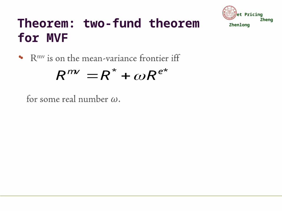
Asset Pricing Zheng ZhenlongTheorem: two-fund theorem
for MVF
• * *mv eR R R

Asset Pricing Zheng ZhenlongProof: Geometric method
* *i e iR R R n
0
R=space of return (p=1)
Re =space of excess return (p=0)
R*R*+wiRe*
Re*
E=0E=1 E=2
Rf=R*+RfRe*
NOTE:1 、回报空间为三维的。 2 、横的平面必须与竖的平面垂直。 3 、如果有无风险证券,则竖的平面过 1 点,否则不过,此时图上的 1 就是 1 在回报空间的投影。
等预期超额收益率线
1

Asset Pricing Zheng ZhenlongProof: Algebraic approach
• Directly from definition, we can get
*
* *
2 2 * * 2
( ) ( ) 0
( ) ( ) ( )
( ) ( ) ( )
0
i e i
i i e
i i e i
i
E n E R n
E R E R w E R
R R w R n
n
=
只有 时,方差在收益率给定情况下才最小。

Asset Pricing Zheng Zhenlong
Decomposition in mean-variance space• *R
)()()()( 22*22*2 ie nEREwRERE

Asset Pricing Zheng Zhenlong
Remark
• The minimum second moment return is not the minimum variance return.(why?)
* 2 2 2 2 2 2( ) ( )OR E E E R E E R
( )R
R*
R*+wiRe*
Ri
E(R)

Asset Pricing Zheng Zhenlong
5.4 Spanning the mean variance frontier

Asset Pricing Zheng Zhenlong
Spanning the mean variance frontier• With any two portfolios on the frontier. we can
span the mean-variance frontier.• Consider
/
)1()(
,
,0,
*****
**
**
wy
yRRyRRw
RwRR
RRR
RRR
e
e
e

Asset Pricing Zheng Zhenlong
5.5 A compilation of properties of R*, Re*, and x*

Asset Pricing Zheng ZhenlongProperties(1)
• Proof:
,)(
1)(
2*2*
xERE
)(/1)(
)()(
,)(
,)(
2*2*
**2*
2*
**2*
2*
**
xExE
RxERE
xE
RxR
xE
xR

Asset Pricing Zheng ZhenlongProperties(2)
• Proof:)( 2*
**
RE
Rx
)()(
,)(
2*
*2***
2*
**
RE
RxERx
xE
xR
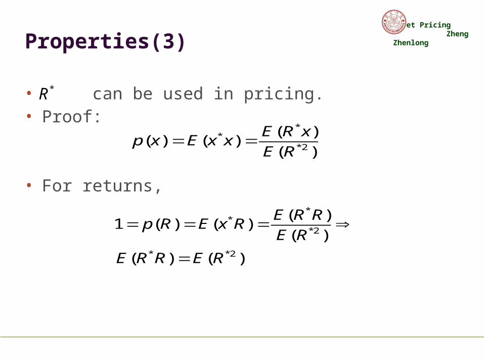
Asset Pricing Zheng ZhenlongProperties(3)
• can be used in pricing.• Proof:
• For returns,
*R
)(
)()()(
2*
**
RE
xRExxExp
**
*2
* *2
( )1 ( ) ( )
( )
( ) ( )
E R Rp R E x R
E R
E R R E R

Asset Pricing Zheng Zhenlong
Properties(4)
• If a risk-free rate is traded,
• If not, this gives a “zero-beta rate” interpretation.
*2
* *
1 ( )
( ) ( )f E RR
E x E R

Asset Pricing Zheng Zhenlong
Properties(5)
• has the same first and second moment.• Proof:
• Then
* * * *2( ) ( ) ( )e e e eE R E R R E R
*eR
))(1)(()()()var( **2*2** eeeee RERERERER

Asset Pricing Zheng ZhenlongProperties(6)
• If there is risk free rate,
• Proof:
** eff RRRR
*
* * *
*
* *
1 (1| ) (1| )
11 (1| ) 1
e
e
f
f
ef f f
proj R proj R
R proj R RR
R R R R
(从上图的两个相似三角形可以看出)
注意R前面的1和R 都是标量,其余都是向量
(这里的第二个R 是标量,其余都是向量)

Asset Pricing Zheng ZhenlongIf there is no risk free rate
• Then the 1 vector can not exist in payoff space since it is risk free. Then we can only use
*
*
* *
* *
**
*2
(1| ) ( (1| ) | ) ( (1| ) | )
(1| ) (1| )
(1| ) (1| )
(1| ) )
( )(1| )
( )
e
e
e
proj X proj proj X R proj proj X R
proj R proj R
R proj X proj R
proj X R
E Rproj X R
E R
= -E(x
= -

Asset Pricing Zheng ZhenlongProperties(7)
• Since
• We can get
* 1
* * *
' ( ')
( ) ( )
x p E xx x
p x E x x
pxxEp
xxxEp
xp
xR
1
1
*
**
)'('
''
)(

Asset Pricing Zheng ZhenlongProperties(8)
• Following the definition of projection, we can get
• If there is risk free rate,we can also get it by:
* ' 1(1| ) ( ) ' ( )e e e e e eR proj R E R E R R R -
pxxEp
xxxEp
RR
RR
ff
e1
1**
)'('
)'('11
11

Asset Pricing Zheng Zhenlong
5.6 Mean-Variance Frontiers for Discount Factors: The Hansen-Jagannathan Bounds

Asset Pricing Zheng Zhenlong
Mean-variance frontier for m: H-J bounds
• The relationship between the Sharpe ratio of an excess return and volatility of discount factor.
• 从经济意义上讲, m 的波动率不应该太大,所有夏普比率也不应太大。
• If there is risk free rate,
)(
|)(|
)(
)(
,1|)()(
)()(|||
,0)()()()()(
,
,
e
e
e
e
Rm
e
Rm
ee
R
RE
mE
m
Rm
REmE
RmREmEmRE
e
e
fRmE /1)(
Asset Pricing Zheng ZhenlongRemark
• We need very volatile discount factors with a mean near one to price the stock returns.

Asset Pricing Zheng Zhenlong
The behavior of Hansen and Jagannathan bounds
• For any hypothetical risk free rate, the highest Sharpe ratio is the tangency portfolio.
• Note: there are two tangency portfolios, the higher absolute Sharpe ratio portfolio is selected.
• If risk free rate is less than the minimum variance mean return, the upper tangency line is selected, and the slope increases with the declination of risk free rate, which is equivalent to the increase of E(m).

Asset Pricing Zheng Zhenlong
The behavior of Hansen and Jagannathan bounds• On the other hand, if the risk free rate is
larger than the minimum variance mean return, the lower tangency line is selected,and the slope decreases with the declination of risk free rate, which is equivalent to the increase of E(m).
• In all, when 1/E(m) is less than the minimum variance mean return, the H-J bound is the decreasing function of E(m). When 1/E(m) is larger than the minimum variance mean return, the H-J bound is an increasing function.

Asset Pricing Zheng Zhenlong
Graphic construction
E(R)
( )m
)(R
)(/)( mEm
1/E(m)
E(m)
( ) / ( )e eE R R

Asset Pricing Zheng ZhenlongDuality
• A duality between discount factor volatility and Sharpe ratios.
{ } { }
( ) ( )min max
( ) ( )e
e
eall m that price x X all excess returns R in X
m E R
E m R

Asset Pricing Zheng ZhenlongExplicit calculation
• A representation of the set of discount factors is
• Proof:
0)(,0)(),',cov(
,)]([)]()([)( 1
xEExx
xExxEmEpmEm
pxEmEpxEmE
xxExExEmEpxEmE
xxExxEmEpmEEmxE
)()()()(
]))([()]()([)()(
)))]([)]()([)((()(1
1

Asset Pricing Zheng Zhenlong
An explicit expression for H-J bounds
• Proof:
))()(())'()(()( 12 xEmEpxEmEpm
( ) ( ) ( )
( ) ( ) ( ) ( )( ) ( ) ( ) ( )
2'
2 1 2
'1 2
'1
( )
( )
m p E m E x
p E m E x p E m E x
p E m E x p E m E x
s s e
s e
-
-
-
æ öé ù ÷ç= - +÷çê ú ÷çë ûè øé ù é ù= - - +ê ú ê úë û ë ûé ù é ù³ - -ê ú ê úë û ë û
å å
åå

Asset Pricing Zheng Zhenlong
Graphic Decomposition of discount factor
* *m x e n
0
M=space of discount factors
E =space of m-x*
x*
x*+we*
e*
E()=0E()=1 E()=2
NOTE: 横的平面必须与竖的平面垂直。
X=payoff space
1Proj(1lX)

Asset Pricing Zheng ZhenlongDecomposition of discount
factor
•
* *m x we
nwexm **
* 1 (1| ) (1| )e proj X proj E

Asset Pricing Zheng ZhenlongSpecial case
• If unit payoff is in payoff space,
• The frontier and bound are just • And
• This is exactly like the case of state preference neutrality for return mean-variance frontiers, in which the frontier reduces to the single point R*.
*m x
* 1 (1| ) 0e proj X
)()( *22 xm

Asset Pricing Zheng ZhenlongMathematical construction
• We have got
( ) ( )( )( ) ( ) ( )
( ) ( )( ) ( ) ( ) ( )( ) ( ) ( ) ( )
* * *
1
1 1
' 1
' 1*
' 12 *
' ' 1 1|
' ' 1 ' '
'
'
cov '
m x we
p E xx x w proj X
p E xx x w E x E xx x
w p wE x E xx x
E m w p wE x E xx E x
m p wE x xx p wE xs
-
- -
-
-
-
= +
= + -æ ö÷ç= + - ÷ç ÷è ø
é ù= + -ê úë ûé ù= + -ê úë û
é ù é ù= - -ê ú ê úë û ë û
Asset Pricing Zheng ZhenlongSome development
• H-J bounds with positivity. It solves
• This imposes the no arbitrage condition.• Short sales constraint and bid-ask spread is
developed by Luttmer(1996).• A variety of bounds is studied by Cochrane and
Hansen(1992).
2min ( ), . . ( ), 0,m s t p E mx m E m 固定

Asset Pricing Zheng Zhenlong