Asset Pricing with Learning about Disaster Risk Yang.pdf · Asset Pricing with Learning about Disaster Risk ... This paper studies asset pricing in an endowment ... where the most

Asset Pricing with Learning about Disaster Risk

– Preliminary and Incomplete –

Yang K. Lu∗ Michael Siemer†

August 2011

Abstract

This paper studies asset pricing in an endowment economy with rare disasters. Existingliterature on rare disaster models generally assumes complete information about disasters.This literature is able to match a large range of asset pricing moments but can only generatetime-varying risk premia under the assumption of exogenous variation in disaster probability.We extend this literature to allow for two sources of uncertainty about a rare disaster: (1) thelack of historical data for a rare disaster results in unknown parameters of the disaster process;(2) the occurrence of a rare disaster takes time to unfold and is thus unobservable directly.We show that when agents employ Bayesian learning rules, learning endogenously introducestime-varying risk premia: Time variation of beliefs generates time variation in returns and themodel can hence better explain large stock market movements during recessions even in theabsence of disasters. Feeding U.S. consumption data of the 20th century into the model showsthat the model improves significantly on matching equity returns relative to a model withoutlearning and illustrates how the disaster belief varies over time. The framework allows us toreconcile the widely held belief during the recent financial crisis that the economy might beat the onset of another great depression.

Keywords: rare events, disaster, Bayesian learning, time-varying risk premia

∗Hong Kong University of Science and Technology. Address: Department of Economics, Clear Water Bay,Kowloon, Hong Kong. Email: [email protected]; http://ihome.ust.hk/∼yanglu/.†Boston University. Address: Department of Economics, 270 Bay State Road, Boston MA 02215. Email:

[email protected]; http://www.michael-siemer.org. The authors are indebted to Francois Gourio and RobertG. King for continuing discussion and support. The authors would like to thank Stelios Bekiros, Vladimir Yankovfor useful comments and suggestions, and participants at the BU macro lunch graduate workshop, the Max WeberFellows June Conference, the Shanghai University of Finance and Economics and the Midwest Macro Meeting 2011.Lu and Siemer gratefully acknowledge the hospitality of Study Center Gerzensee, Switzerland.

1

1 Introduction

Why are the stock returns so high and so volatile? It is a classic question in both economics and

finance. This paper attempts to answer this question by developing a consumption based learning

model in which agents learn about rare events that affect the dividends.

In an endowment economy, a rare disaster is defined as some infrequently occurring event with

a long-lasting negative effect on consumption growth. The majority of existing literature on rare

disaster models generally assumes that the entire damage caused by a rare disaster occurs over

a single time period, and that agents have complete information about the disaster. We model

disasters in a more realistic way, following Barro, Nakamura, Steinsson and Ursua (2011), that the

disaster unfolds over multiple periods. We also extend Barro et al. (2011) to allow for two sources

of uncertainty about a rare disaster: (1) whether a disaster has occurred is not directly observable

since its effects take time to unfold; (2) how much damage a disaster will cause is governed by

some unknown parameters due to the lack of historical data for such a rare event. The evidences

for these two types of uncertainty are apparent in the empirical results of Barro et al. (2011). The

estimated posterior beliefs of being in a disaster vary significantly as illustrated in Figure IV of

their paper. The estimated standard deviations of the short-run and the long-run shocks during

disasters are large, revealing that there is a great amount of uncertainty during a disaster about

its short-run and long-run effects.

Agents in our model observe real-time data on consumption and update their beliefs about the

occurrence and the severity of a disaster over time. Learning implies time-varying risk premium

endogenously because the time variation of beliefs generates time variation in how risky the current

economy is as perceived by agents. Since it is not directly observable whether a disaster occurs,

agents can sometimes mistake a recession for the beginning of a rare disaster. For example,

during the recent financial crisis, many commentators, including well-known macroeconomists,

have highlighted the possibility that the U.S. economy could fall into another Great Depression

and the market reacted with a large drop in stock prices and an increase in volatility. Misperceived

risk of a rare disaster may explain why agents overreact to some shocks, which, in retrospect,

2

should not have generated such turmoil. Hence, our model can generate time-vary risk premium

even in the absence of a disaster. Conditional on being in a disaster, agents also need to learn how

the disaster will develop from real-time data. In turn, risk premium is also time-varying during

disaster periods.

Since the second half of the twentieth century features no disasters for the U.S., the ability of

generating large stock market movements during normal recessions lends our model an advantage,

relative to much of the literature on learning and asset prices, in obtaining many of the asset

pricing facts without assuming excessively large levels of risk aversion or leverage.

Furthermore, the fact that the time-variation in stock returns is endogenous in our learning

model enables us to make further progress in two important areas in the asset pricing literature:

1) explaining the predictive regressions that commonly use dividend-price ratio as a predictor for

future excess returns and dividend growth; 2) interpreting historical consumption and stock price

data.

Starting with Campbell and Shiller (1988) and Fama and French (1988), predictive regressions

become common in asset pricing literature. However, the current literature on disaster risk is silent

on this aspect of empirical evidences since it suffers from one of the following two problems. First,

many models including Barro (2006) and Barro et al. (2011) imply a constant dividend-price ratio

during non-disaster periods. This makes it impossible for the dividend-price ratio to predict time

varying returns since disasters are rare events and most of the time the economy is not in a disaster

state. Second, models such as Gabaix (2008) and Gourio (2011) feature time-varying dividend-

price ratios during non-disaster periods purely due to the exogenous time variation in risk. This

feature again deprives the dividend-price ratio of its predictability for future returns. In addition,

what remains unexplained in these papers is the fundamental driving force behind the time-varying

disaster probability. In this paper, learning is explicitly modeled so that agents’ learning about

the occurrence and the severity of a rare disaster endogenously generates time-variation in the

perceived risk of a disaster and, in turn, in both dividend-price ratios and equity returns. In this

sense, our model provides a foundation for why the disaster probability can be assumed to be

3

time-varying. At the same time, it also contributes to understanding the predictability in the data

(see also Brandt et al.,2004 and Cogley and Sargent, 2008).

Finally, our model is built in a way that agents learn from observing data on consumption

growth. Hence, we can feed our model with actual consumption data following Campbell and

Cochrane (1999). Cyclical variations in consumption growth will induce agents in the model to

learn and update their beliefs about disasters, which will in turn imply a time series of equity

returns. We can then compare historical data on equity returns with the model-implied ones, as a

test for the performance of our model.

1.1 Literature Review

It is well-known that there is a long list of stock market and bond market puzzles in macro-

finance literature. Among them, time-varying risk premium have received a great amount of

attention since Cochrane (1999). Three main classes of rational expectation models have been

proposed to generate time-varying risk premium. First, there are models based on habit formation

where the most successful work is Campbell and Cochrane (1999). With habit being a weighted

average of past aggregate consumption, this type of model is able to generate time-varying risk

premium endogenously. Earlier important work in the habit literature include Constantinides

(1990), Sundaresan (1989) and Abel (1990). The second type of models is in the long-run risk

literature, such as Bansal and Yaron (2004) and Bansal, Kiku and Yaron (2010). The combination

of an unobservable long-run component in the consumption growth process, the presence of a

predictable long-run component and Epstein-Zin preferences leads to the rise of time varying risk

premium.

The third strand is the disaster literature with time varying disaster probability.1 Following the

seminal papers by Rietz (1988) and Barro (2006), an emerging literature has developed to study

the effect of rare disasters on asset markets and on business cycles. Existing work has proven that

having potential disasters is a powerful way to generate large risk premium. Examples include

1Alternatively disaster probability can be constant if disaster size is time varying.

4

Liu, Pan and Wang (2005), Farhi and Gabaix (2008), Gabaix (2008), Gourio (2008a,b), Wachter

(2008), Backus, Chernov and Martin (2009), Barro and Ursua (2009), Bates (2009), Bollerslev and

Todorov (2009), and Santa-Clara and Yan (2009). However, only a few manage to reproduce the

dynamics of risk premium, which requires time-variation in either the quantity or the price of risk.

Time-variation is frequently generated by assuming that the probability of disaster is time-varying

as in Wachter (2008), Gabaix (2008) and Gourio (2011).

Introducing learning into models of asset pricing and macroeconomics has been remarkably

successful in fitting the persistence and volatility of asset returns and business cycle movements, as

compared to rational expectation models. Two main sources of uncertainty are generally used to

motivate learning: 1) some parameters of the economic model are unknown to agents (see Evans

and Honkapohia, 2001 for a survey); and 2) a state – typically a regime or a permanent component

in a shock – is not directly observable to agents.

It is typical for a learning model to employ only one source of uncertainty. Parameter uncer-

tainty is shown to be important to explain stock returns, see for examples, Timmermann (1996,

2001) and Weitzman (2007). State uncertainty, through learning, motivates and disciplines time-

varying risk premium, e.g. Veronesi (1999, 2004), Chen and Pakos (2007). However, focusing on

only one source of uncertainty limits the explanation power of a model. Without state uncer-

tainty, parameter uncertainty will die out in the long run as more data is accumulated and agents

are increasingly confident about their estimates for the constant parameters. Without parameter

uncertainty, learning the hidden state tends to be too fast to play an important role in explain-

ing time-varying risk premium, given the limited variability of observed consumption, output or

dividend process, which typically serves as a noisy signal for the hidden state.

A unified framework to study jointly parameter and state uncertainty is thus promising in

bringing the learning models closer to the data. However, very little work has been done so far

on this front. One pioneer paper is Lewis (1989), which shows that a simple learning model in

the presence of these two sources of uncertainty is capable to explain the behavior of U.S. dollar–

German mark forecast errors during the early 1980’s. This paper pushes further in developing the

5

unified learning framework given that learning about a rare disaster is a natural combination of

parameter and state uncertainty: 1) the lack of ex-ante knowledge of a rare disaster forces agents

to learn its unknown parameters; and 2) the occurrence of a rare disaster is unobservable directly

and is in turn a hidden state.

In modeling the parameter uncertainty, we are taking a consistent approach between the learn-

ing and how the learning maps to the market outcomes. In other words, our agents are rational

learners so they takes into account the parameter uncertainty in pricing assets. Although this idea

of rational learning is widely adopted in the learning literature,2 we are the first - to the best of our

knowledge - to implement it in a model with both parameter uncertainty and state uncertainty.

In a related study by Johannes, Lochstoer and Mou (2010) where the two-sided uncertainties are

also present, agents are assumed to ignore the parameter uncertainty in pricing the assets. To

investigate the impact of this simplification assumption, we also compute asset returns under this

assumption and contrast them with the ones computed using the fully rational approach. We find

that ignoring the parameter uncertainty in asset pricing significantly overstates the volatility of

returns.

2 The Model

This section presents the baseline model and explains how the model agents update their beliefs.

2.1 Consumption process with rare disasters

We adopt the following process for consumption growth in which disasters affect long run consump-

tion growth. For a realistic modeling we follow Barro et al. (2011) and allow for time variation in

the disaster realization θt

∆ logCt = ct = µ+ Itθt + ηt (2.1)

2Townsend (1978), Wieland (2000a, 2000b), Guidolin and Timmermann (2007), Cogley and Sargent (2008).

6

This process captures two features of a disaster: 1) a disaster typically lasts for several periods;

and 2) each disaster is unique in terms of its long-run damage.

The log consumption in the expression above follows a random walk with a state-dependent

drift. When a disaster occurs at period t, It = 1, otherwise, It = 0. It follows a Markov chain with

transition probabilities: Prob(It+1 = 1|It = 0) = p and Prob(It+1 = 0|It = 1) = 1− q.

In the absence of a disaster, the economy’s consumption growth rate is exposed to i.i.d. shock,

ηt. ηt is normal with mean zero and variance σ2η. When a disaster occurs, θt represents the long-run

drop in consumption. θt is a random draw from a normal distribution F (θ) in the period when a

disaster starts and is constant for one disaster episode – consecutive periods with It = 1. Therefore,

θt is different across different disaster episodes, but is constant during each disaster realization.

2.2 Bayesian Learning

Agents in the model are Bayesian learners. Agents observe the consumption process ct ≡ {cs}ts=0

at t but do not observe It and θt. The agents thus face two uncertainties: textitstate uncertainty

which is referring to the unobserved disaster realization It and parameter uncertainty referring to

the unobserved θt.

The two-sided uncertainty distinguishes our model from the existing literature on models with

learning, where typically only one kind of uncertainty is present. With perfect knowledge of θt

and only uncertainty about It, the model reduces to a standard hidden Markov regime switching

model. With perfect knowledge of the disaster state It and only uncertainty about the disaster

severity θt, the model fits into the familiar framework of adaptive learning.

Conditional on θt and It, the likelihood function for consumption growth ct is the density

function for a normal random variable. The likelihood function for ct can be combined with Bayes’

rule to update agents’ belief about the disaster state, It, (the disaster parameter, θt) conditional

on perfect knowledge of the disaster parameter, θt (the disaster state It).. However, if agents have

to learn both – state and parameter – the simple Bayes’ updating rule does not apply any longer.

The next section explains in detail how agents update their belief in a world

7

2.2.1 Learning the State under Parameter Uncertainty

Without perfect knowledge of θt, the posterior belief of It, Pr (It = 1|ct), can still be obtained by

integrating out θt from its conditional information set, as long as agents have a belief about θt.

The resulting likelihood function of ct is independent of a particular θt consequently becomes

Pr(ct|It−1 = i, It = j, ct−1

)=

∫θ

Pr (ct|θt, It) Pr(θt|It−1, It, ct−1

)dθt. (2.2)

We can then obtain the posterior belief of It using Bayes’ rule after combining the likelihood

function above with the prior belief of It:

Pr(It = 1|ct

)=

∑i=0,1 Pr (ct|It−1 = i, It = 1, ct−1) Pr (It−1 = i, It = 1, |ct−1)

Pr (ct|ct−1). (2.3)

Now we turn to how to obtain the posterior belief about the disaster parameter θt.

2.2.2 The Learning Switch

Each time a disaster starts, the parameter θtis drawn from F (θt)and will remain constant until

the end of this particular disaster. Thus, agents’ belief about θt has to be conditioned on the state

of the economy. However, since agents in our model never know the disaster state perfectly, the

number of possible disasters will grow with the number of periods, so does the number of possible

θts that agents have to form belief about. The exploding number of beliefs about different θts

over time make this problem untractable. To resolve this issue, we put more structure on how

agents update their beliefs and introduce an instrument called ”learning switch”. That is, agents

do not continuously update their belief about being in a disaster but only activate learning if it

is triggered through by a significant event. One example for such a significant event could be the

collapse of Bear Stearns and Lehman Brothers in the fall of 2008.

Definition. The learning switch is an indicator that can take two values: ’off’ or ’on’. When the

learning switch is off at period t, agents are perfectly sure that It−1 = 0. When the learning switch

is on at period t, agents learn over time whether a disaster occurred at the most recent date when

8

the learning switch was turned on.

By defining the learning switch, we are actually making several assumptions about agents’

beliefs, which are now listed explicitly as follows.

Assumption 1. If the learning switch is off, agents ignore the slight chance that the economy may

be in a disaster state.

The basic idea behind the ”learning switch” is that agents are not always suspicious about

whether the world today is in a disaster, unless they observe some evidence about it. We view it

as a reasonable assumption since it would be absurd for agents to think they are currently in a

disaster (or a depression) when the economy is booming.

Therefore, the implication of the learning switch being off at period t is that there are only

two possibilities of the disaster states: a) no disaster: It−1 = 0, It = 0 and b) a disaster occurs:

It−1 = 0, It = 1.

Assumption 2. If the learning switch is on, agents believe that the disaster can only start at the

latest date when the learning switch is turned on.

This belief is reasonable in the sense that if agents are still wondering whether a disaster has

occurred, it is very unlikely for them to start contemplating whether a disaster had occurred but

was already finished and also followed by a new disaster. Note that this restriction on belief does

not rule out the event of two consecutive disasters (say, double-dip). If agents learn a disaster has

never occurred or a disaster has ended (when we define the learning trigger to be off), they are

alerted that a new disaster may start at any date.

Under this assumption, there are only three possibilities of the disaster states when the learning

switch is on at period t: a) a disaster never occurs: It−1 = 0, It = 0; b) A disaster occurred and

continues: It−1 = 1, It = 1; c) a disaster occurred but ends: It−1 = 1, It = 0.

An immediate implication of excluding (It−1 = 0, It = 1) is on the transition matrix that agents

use during the learning-switch-on period: Prob(It = 1|It−1 = 0) = 0 and Prob(It = 0|It−1 = 1) = q.

9

Assumption 3. If agents do not observe strong evidence that a disaster ends at t, they think for

sure that the disaster continues, conditional on it ever occurring.

Conditional on a disaster occurring, agents’ beliefs about its specific parameter θt are updated

over time and they have a more precise idea about θ towards the end of the disaster than they do

at the beginning. This better knowledge makes detecting the end of a disaster significantly easier.

Thus, this assumption echoes Assumption 1 in the sense that agents ignore the possibility of an

event (that a disaster may start or end) if they do not see strong evidence of it.

Now that the learning switch is defined, it needs to be explained under what conditions agents

turn learning on or off. We follow the approach by Marcet and Nicolini (2003) to use likelihood

ratio as a way to define ”evidence”.

When the learning switch is off at period t, it can be turned on by evidence in period t, if

Pr (It−1 = 0, It = 1|ct)Pr (It−1 = 0, It = 0|ct)

> Ton (2.4)

In this case, the learning switch at period t+ 1 is set to be on.

When the learning switch is on at period t, it can be turned off by evidence at period t, if

agents

1) learn that a disaster never occurs:


> T 0off (2.5)

2) learn that a disaster ends:


> T 1off (2.6)

In this case, the learning switch at period t+ 1 is set to be off.

10

2.2.3 Learning the Parameter θt

After introducing the learning switch, we will be able to reduce the prior belief about the disaster

parameter, θt, down to only two versions, priornd(t) and priord(t), associated with It−1 = 0 and

It−1 = 1, respectively.

When the learning switch is off at both t and t+1, that is agents know for sure It−1 = 0, It = 0,

priornd(t) is updated to priornd(t+ 1) when combined with the likelihood function of ct.

When the learning switch turns from off to on (t to t + 1), agents are no longer sure whether

there is a new disaster at t, so priornd(t) is updated to priornd(t+ 1) and priord(t+ 1) depends

on It = 0 or 1.

When the learning switch is on at both t and t+ 1, there are three possibilities:

1. Conditional on It−1 = 0, It = 0, priornd(t) is updated to priornd(t+ 1).

2. Conditional on It−1 = 1, It = 1, priord(t) is updated to priord(t+ 1).

3. Conditional on It−1 = 1, It = 0, we do not carry along the updated prior because this

possibility is excluded if evidence that a disaster ends is not strong enough to turn the learning off

at t+ 1.

When the learning switch turns from on to off (t to t + 1), agents are sure that It = 0.

priornd(t+ 1) is then updated from priornd(t) if agents learnt that a disaster never occurs, and

from priord(t) if agents learnt that a disaster occurs but ends at t.

Conditional on It−1, It, the posterior belief of θ can be updated using the latest data ct:

Pr(θ|It−1, It, ct

)=

Pr (ct|θ, It) Pr (θ|It−1, It, ct−1)Pr (ct|It−1, It, ct−1)

. (2.7)

The prior belief about θ has to be conditional on (It−1, It) because when (It−1 = 0, It = 1), a new

disaster starts and θ will be a new draw from its unconditional distribution, which implies:

Pr(θ|It−1 = 0, It = 1, ct−1

)= f (θ) . (2.8)

11

In other cases, the prior belief about θ is the posterior belief inherited from last period:

Pr(θ| (It−1, It) 6= (0, 1), ct−1

)= Pr

(θ|It−1, ct−1

)(2.9)

3 Asset Pricing

We study an endowment economy following Mehra and Prescott( 1985) with only two assets: one

is the risk free asset with return Rft+1, and the other is an equity that claims the next period

consumption:

Ret+1 = (Pt+1 + Ct+1) /Pt. (3.1)

The utility function of agents is Epstein-Zin (EZ) with γ being the coefficient of relative risk

aversion and ψ being the inter-temporal elasticity of substitution (IES). The time discount factor

is β.

3.1 Asset Pricing with Perfect Information

Under EZ utility, if agents can observe θt and It perfectly, we know that the price-dividend ratio,

Pt/Ct, is a function f (θt, It) – PDR function – which satisfies the following Euler equation.

(Pt/Ct)ε = βEt

[(Ct+1/Ct)

ε(ψ−1)ψ (Pt+1/Ct+1 + 1)ε

]so that:

f (θt, It) = β

{Et

[exp

(ε (ψ − 1)

ψct+1

)[f (θt+1, It+1) + 1]ε

]}1/ε

(3.2)

where ε = (1− γ) (1− 1/ψ)−1.

After obtaining the price-to-dividend ratio, the returns of two assets are simply:

Rft+1 (θt, It) =

[βεEt exp

((ε (ψ − 1)

ψ− 1

)ct+1

)[f (θt+1, It+1) + 1

f (θt, It)

]ε−1]−1Ret+1 (θt+1, It+1) =

f (θt+1, It+1) + 1

f (θt, It)exp (ct+1)

12

3.2 Asset Pricing with Imperfect Information

However, neither θt nor It is directly observable, so we have to replace them in the PDR func-

tion f (θt, It) by the corresponding agents’ beliefs, Pr (θt|It = 0, ct), Pr (θt|It = 1, ct) and Pr (It|ct).

Pr (θt|It, ct) is normal distribution and thus can be summarized by its mean and variance. Pr (It|ct)

is a scalar variable. The PDR function under imperfect information, F [Pr (θt|It, ct) ,Pr (It|ct)],

needs to satisfy:

F[Pr(θt|It, ct

),Pr

(It|ct

)]= β

{Et

[exp

(ε (ψ − 1)

ψct+1

){F[Pr(θt+1|It+1, c

t+1),Pr

(It+1|ct+1

)]+ 1}ε

]}1/ε

.

In addition to replacing (θt, It) by the beliefs, imperfect information about θt and It also changes

the expectation formation Et. In particular, conditional on the information set at period t, the

distribution of future ct+1 = µ + It+1θt+1 + ηt+1 is determined by Pr (θt|It, ct) and Pr (It = 1|ct)

due to the persistence of θt and It. Each future data ct+1 implies a set of updated state variables,

Pr (θt+1|It+1, ct, ct+1) and Pr (It+1 = 1|ct, ct+1), which are in turn associated with a particular future

PDR. The expectation is taken by averaging across all possible future ct+1 and the associated PDRs.

We leave the details of the PDR computation to the Appendix. A similar methodology applies to

the computation of the risk free rate.

To the best of our knowledge, this is the first paper that treats the belief about the parameter

- a distribution - as the state variable in the PDR function. A typical approach in existing asset

pricing models with parameter uncertainty is to assume that agents are adaptive learners in the

sense that they view parameters as constants in forming expectations whereas their beliefs about

parameters are in fact updated over time when new data comes in [e.g. Johannes et al. (2010)]. Our

model setup allows us to overcome this inconsistency between expectation formation and learning

so our agents are fully Bayesian. This new approach thus takes full account of how parameter

uncertainty affects asset returns.

In order to better understand the implications of this new approach on asset returns, we also

13

compute asset returns using two alternative approaches with restrictive assumptions imposed at

various steps during the computation. The first approach is the common one taken in the existing

literature, where θ is fixed at the level of its posterior mean during the PDR computation. The

second approach uses the posterior belief about θ in determining the distribution of future ct+1

but does not update the posterior belief about θ with each ct+1 in evaluating the next-period

price-dividend ratio.. We view the second approach as a step in between the first approach and

the benchmark one since this approach does take into account the belief about θ but treats it as

fixed rather than a state variable.

Another novelty of our model is the presence of the dual uncertainties, namely parameter

uncertainty and state uncertainty, in agents’ learning. To gain a better understanding of its

impact, we compute asset returns under three information structures: The first scenario is no

learning where agents have perfect information about the current and past states of the economy

(Is)ts=0. We first assume that agents also have perfect information about the future θs so that there

is no uncertainty in the model. Then we assume agents view the parameter θ as a new draw from

the distribution F (θ) each period. This case shuts down the learning and is designed to capture

the effect of parameter uncertainty on asset returns. The second scenario is partial learning where

agents learn about the disaster state It conditional on the knowledge of θ.3 This case shows the

effect of state uncertainty on asset returns and is one of the well-known hidden Markov regime

switching models. The third scenario is our benchmark case – joint learning – where agents have to

learn jointly the parameter θ and the state It. Parameter uncertainty and state uncertainty interact

with each other in this case and the interaction has important implications for asset returns.

3.3 Calibration

All our results are computed with the same parameter values as reported in Table 1. We set the

values of the parameters governing consumption process equal to the posterior means estimated

3Another case of partial learning is to let agents learn the parameter θ conditional on their perfect knowledgeof the state It. But this case is equivalent to the no learning case with a time-varying F (θ), so we omit it in ourcomputation.

14

in Barro et al. (2011) whenever possible. The time period is one year. Because the equity return

is a leveraged claim on the consumption stream in reality, we compute levered equity return with

the leverage parameter λ set to 2.4 The preference parameters are standard with a rather low risk

aversion coefficient of 6.5, the IES equal to 2. Risk aversion is picked to match the equity return

in the benchmark case. An extensive debate evolves around the values of the IES. It is crucial for

our model - as for most successful asset pricing models - to have an IES larger than one. We set

the time discount factor, β, equal to 0.978. The discount factor is picked to roughly match the

risk free rate in our benchmark model. The only two free parameters in our learning model are

two thresholds governing the learning switch. Ton = 0.015 means that the learning switch will be

turned on when the probability of a new disaster today is 1.5% of the probability of no disaster

today. This implies our agents are quite alerted by the possibility of a new disaster. Toff = 50

means that the probability of no disaster today needs to be 50 times larger than the probability

of a disaster continuing in order to turn the learning switch off. This implies a dominant evidence

is required to assure our agents that there is no need to worry about being in a disaster today.

Given the relative arbitrary Ton and Toff , we compute our joint learning model under alternative

choices of Ton and Toff . The asset returns are of course sensitive to the choices since the number

of periods when agents are learning varies, but all the major results are robust within a reasonable

range of Ton and Toff . Results for robustness checks can be found in the Appendix.

[Table 1 about here.]

4 Results in an endowment economy

In this section, we report asset returns in the models with no learning, partial learning and joint

learning, respectively. In the no learning model, we first compute asset returns with ”no uncer-

tainty” about either the parameter or the state, and then we compute asset returns with only

parameter uncertainty present. In contrast, the partial learning model only has state uncertainty.

4There is no consensus in the literature about the level of leverage. Typically the parameter value ranges from1.5 to 4. [see Barro et al. (2011), Gourio (2011), Bansal and Yaron (2004)]. We take a conservative view and setthe leverage parameter equal to 2.

15

In the joint learning model, we compute the PDR function following three different approaches: 1)

our benchmark approach (”dist state”) in which the distribution of θ is treated as a state variable;

2) an intermediate approach (”fix dist”) in which the distribution of θ is fixed to agents’ posterior

belief; and 3) the common approach (”fix mean”) in the literature that fixes the parameter θ at

its posterior mean.

We further group those results into three sets. The first set of results shows the behavior of

equity returns and risk free rates when a disaster occurs. The second set of results reports the

statistics of asset prices in a sample without any realization of disasters. The third set of results

looks at how our model fits the historical consumption and stock return data.

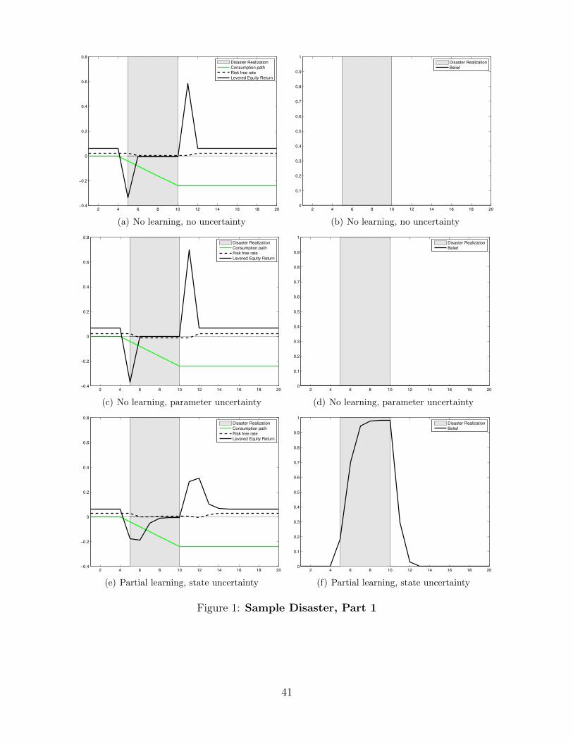
4.1 Returns over a Sample Disaster

In this subsection, we investigate the dynamics of asset returns with a sample disaster starting at

period 5 and lasting for 6 periods (years). The long-run damage on consumption growth of this

particular disaster is set to be 4% each period during the disaster, which implies a total 24% drop

of consumption in the long run. All the shocks ηt are set to zero.

[Figure 1 about here.]

The left panels of Figure 1 and Figure 2 display the asset returns computed in the aforemen-

tioned 6 cases under EZ utility. The black solid line is the time series of equity returns and the

black dashed line is the time series of risk free rates. The green line reflects the de-trended logCt

path. The right panels of Figure 1 and Figure 2 display the dynamics of agents’ belief of being in

a disaster.

A general pattern across the return graphs is that the stock market crashes at the onset of the

disaster and booms after the disaster ends. What differs across various cases are the magnitude

and the persistence of crash and the boom.

Let us first look at the case under no learning. Comparing asset returns with and without

parameter uncertainty, it is clear that the parameter uncertainty increases the equity returns and

lowers the risk free rate. The intuition is quite straightforward in a world with risk-averse investors.

16

The exposure of equity to the extra risk implied by the parameter uncertainty raises the demand

of risk-free asset and suppresses the demand of equity. Therefore, the risk-free asset yields lower

return and the risky asset needs to be compensated with higher return. In addition, the stock

market crash is more severe in the case with parameter uncertainty since in the disaster state, the

exposure to the parameter uncertainty is much larger than in the normal state. It follows that the

equity price plunges deeper at the onset of a disaster when the parameter uncertainty is present.

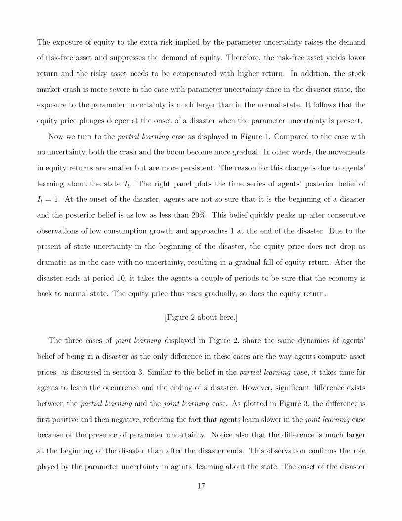
Now we turn to the partial learning case as displayed in Figure 1. Compared to the case with

no uncertainty, both the crash and the boom become more gradual. In other words, the movements

in equity returns are smaller but are more persistent. The reason for this change is due to agents’

learning about the state It. The right panel plots the time series of agents’ posterior belief of

It = 1. At the onset of the disaster, agents are not so sure that it is the beginning of a disaster

and the posterior belief is as low as less than 20%. This belief quickly peaks up after consecutive

observations of low consumption growth and approaches 1 at the end of the disaster. Due to the

present of state uncertainty in the beginning of the disaster, the equity price does not drop as

dramatic as in the case with no uncertainty, resulting in a gradual fall of equity return. After the

disaster ends at period 10, it takes the agents a couple of periods to be sure that the economy is

back to normal state. The equity price thus rises gradually, so does the equity return.


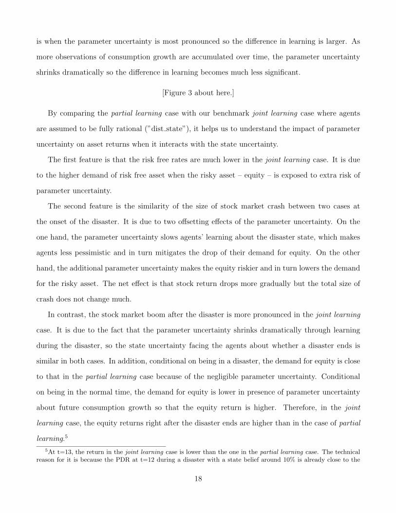
The three cases of joint learning displayed in Figure 2, share the same dynamics of agents’

belief of being in a disaster as the only difference in these cases are the way agents compute asset

prices as discussed in section 3. Similar to the belief in the partial learning case, it takes time for

agents to learn the occurrence and the ending of a disaster. However, significant difference exists

between the partial learning and the joint learning case. As plotted in Figure 3, the difference is

first positive and then negative, reflecting the fact that agents learn slower in the joint learning case

because of the presence of parameter uncertainty. Notice also that the difference is much larger

at the beginning of the disaster than after the disaster ends. This observation confirms the role

played by the parameter uncertainty in agents’ learning about the state. The onset of the disaster

17

is when the parameter uncertainty is most pronounced so the difference in learning is larger. As

more observations of consumption growth are accumulated over time, the parameter uncertainty

shrinks dramatically so the difference in learning becomes much less significant.


By comparing the partial learning case with our benchmark joint learning case where agents

are assumed to be fully rational (”dist state”), it helps us to understand the impact of parameter

uncertainty on asset returns when it interacts with the state uncertainty.

The first feature is that the risk free rates are much lower in the joint learning case. It is due

to the higher demand of risk free asset when the risky asset – equity – is exposed to extra risk of

parameter uncertainty.

The second feature is the similarity of the size of stock market crash between two cases at

the onset of the disaster. It is due to two offsetting effects of the parameter uncertainty. On the

one hand, the parameter uncertainty slows agents’ learning about the disaster state, which makes

agents less pessimistic and in turn mitigates the drop of their demand for equity. On the other

hand, the additional parameter uncertainty makes the equity riskier and in turn lowers the demand

for the risky asset. The net effect is that stock return drops more gradually but the total size of

crash does not change much.

In contrast, the stock market boom after the disaster is more pronounced in the joint learning

case. It is due to the fact that the parameter uncertainty shrinks dramatically through learning

during the disaster, so the state uncertainty facing the agents about whether a disaster ends is

similar in both cases. In addition, conditional on being in a disaster, the demand for equity is close

to that in the partial learning case because of the negligible parameter uncertainty. Conditional

on being in the normal time, the demand for equity is lower in presence of parameter uncertainty

about future consumption growth so that the equity return is higher. Therefore, in the joint

learning case, the equity returns right after the disaster ends are higher than in the case of partial

learning.5

5At t=13, the return in the joint learning case is lower than the one in the partial learning case. The technicalreason for it is because the PDR at t=12 during a disaster with a state belief around 10% is already close to the

18

Putting all the pieces together, the presence of the parameter uncertainty makes equity return

in our benchmark joint learning case more volatile than the one in the partial learning case.

Finally, let us turn to compare three cases with joint learning. Because the three cases share

the same dynamics of beliefs about both the state and the parameter, the differences across asset

returns should be purely due to how the function for the price-dividend ratio is computed. .

In our benchmark joint learning case, agents are fully rational. They not only acknowledge

their imperfect information about θ but also account for future updates in the belief about θ

when pricing the assets. When the PDR function is computed using the intermediate approach

(”fix dist”), agents are myopic in the sense that they ignore changes in their future beliefs and

only account for their current belief about θ in pricing the assets. In the last case where the PDR

function is computed using the common approach (”fix mean”) in the literature, agents completely

ignore the parameter uncertainty about θ in asset pricing and simply adopt their best estimate of

θ (the posterior mean) as the parameter value.

Therefore, the parameter uncertainty embedded in asset pricing is descending when we move

from the benchmark approach to the common approach. Lower parameter uncertainty increases

the demand for equity and in turn raises the PDR and the risk free rate in normal time. When

the disaster starts, parameter uncertainty gets quickly resolved over time so the PDRs in three

cases all drop to a similar low level during the disaster. This implies larger changes of PDR during

the disaster for the case with less uncertainty, and thus more volatile movements of asset returns

during the disaster when we move from the benchmark approach to the common approach.

4.2 Quantitative Results

In this subsection, we simulate a consumption path for 100,000 periods with no disaster realization

throughout. We do this in order to compare the model results to the corresponding moments of

U.S. data from 1948-2009. Clearly, this period did not feature any disasters and thus we need to

level of the PDR in normal time. The intuition is that being in a disaster with a not too bad theta and smallparameter uncertainty is similar as in the normal state but exposed to much higher parameter uncertainty

19

compare it to a simulation without disaster realization.6 This exercise highlights the capability

of our learning model in generating high equity premium and reasonable return variation even

without any realization of disasters, a feature that distinguishes our model from many others in

the literature on rare disasters.

4.2.1 Moments

Table 2 reports the averages and standard deviations of risk-free rates and levered equity returns.

Panel I reports moments from the actual data. We use the U.S. equity return series from the

CRSP database, available on WRDS. Data are annual from 1948 to 2009 and expressed in percent.

The returns from the actual data are thus corresponding to a consumption process without any

realization of disasters.


Panel II reports the corresponding model moments. Rows 1 and 2 reports the moments of

model-implied asset returns in the case of no learning. Consistent with the sample disaster graphs,

parameter uncertainty reduces the risk free rate and raises the equity return. So parameter uncer-

tainty drives up the equity premium but not as much as the one from the actual data. In addition,

without any learning, there is little variation in the equity returns compared to the data.

Row 3 shows the results from the partial learning case. Because there is no disaster realization

in our simulation and in turn no θ realization, we assume that agents in this case view θ equal

to the mean of its unconditional distribution F (θ). Learning adds significant variation in equity

returns compared to the no learning cases. State uncertainty increases equity returns compared

to the case with no uncertainty but not as much as what parameter uncertainty does. This case

illustrates that a standard Markov model typically requires high risk-aversion and high leverage in

order to match equity excess returns.

Row 4 is our benchmark joint learning case. With both parameter and state uncertainty

present, the mean of risk free rate is lower and the mean of equity return is raised by a significant

6Since there is no disaster realization in the simulation, there are no draw for the parameters (θ, φ). Therefore,in computing the case of state learning, we assume that agents think the true (θ, φ) are at their prior means.

20

magnitude, pushing the equity premium closer to the data. The standard deviation of equity

returns also improves compared to the partial learning case, and now counts for more than 40%

of its counterpart in data.7 It is worthwhile to emphasize again that those moments are generated

without any occurrence of disasters in the simulated sample.

Rows 5 and 6 are the results from two alternative approaches of computing PDR functions

in the joint learning case. Borrowing the intuition from the results over a sample disaster, less

uncertainty embedded in asset pricing raises the risk free rate and lowers the equity premium.

The standard deviation of equity returns increases a lot from our benchmark case due to the large

changes in PDRs when switching between low and high consumption growth.

The contrast between row 4 and row 6 clearly shows that the finding of Cogley and Sargent

(2008) does not hold true in the context of our asset pricing model. The authors find that using the

exact Bayesian rule as we do in our benchmark joint learning model gives very similar asset pricing

results as using the anticipated utility framework based on Kreps (1998) that we examine in row

6. On the other hand, our finding is consistent with Guidolin and Timmermann (2007) which also

documents large differences in asset prices between rational learning schemes and myopic-adaptive

shemes. This controversy thus begs the question if adopting rational learning schemes will make

a difference in the models by Johannes et al. (2010) and Piazessi and Schneider(2011) who use

anticipated utility framework in the context of asset pricing.

A number of papers in the literature (e.g. Johannes et al. (2010)) have added an additional

component for computing equity returns. The motivation is that consumption volatility is much

lower than dividend volatility (standard deviation of consumption in our sample is about 1.8% while

standard deviation of dividends in the data is about 11.4%). As the model prices a consumption

7Because the unconditional mean of long-run shock θ is close to the standard deviation of the shock in normaltime, agents are easy to get confused in the partial learning case. In 50% of the time periods, agents think theeconomy is in a disaster state by a chance over 1.5%. The counterpart number in the joint learning case is 16% ofthe time periods. This fact adds more volatility of equity returns in the partial learning case. However, if we wouldtake into account the short-run effect of a disaster, agents will be less confused if they have perfect informationabout the parameters. So the abstraction from short-run effect of a disaster biases our results in favor of the partiallearning case.

21

claim many papers modify the model’s dividend process in the following fashion:

Dt+1

Dt

=

(Ct+1

Ct

)λexp(−0.5σ2

d + σdε) (4.1)

where ε ∼ N(0, 1) and σd then is typically picked to match the volatility of dividends in the

data. Clearly we could add this to our model and dramatically increase the volatility of our equity

returns.

4.2.2 Return Predictability

Following the literature, we run predictive regressions of stock market excess returns on lagged

dividend price ratios from the data and our model:

lnRet→t+k − lnRf

t→t+k = αk + βk ln (Dt/Pt) + εt+k

We run the regressions for each horizon from 1 to 5 years.(k = 1, 2, ...5). Excess market returns

are from Ken French. Dividend-price ratios are backed out from CRSP data. The risk free rate is

from Ibottson.

Table 3 report the slope coefficient βk, and R2 from the regressions. The regression results

using the data in Panel I confirm the general findings in the literature that dividend price ratio

have significant predictive power over future excess returns. Moreover, both coefficient value and

R2 are increasing with the horizon.


The model results are displayed in Panel II. It is not surprising that there is no prediction

power of dividend price ratio in the two no learning cases since the dividend-price ratio is constant

in absence of disaster realizations.

All the cases with learning have positive and significant βk at each return horizon. In addition,

as in the data, βk increases with the return horizon. These results are consistent with the findings by

Timmermann (1993, 1996) that learning effects on stock price dynamics are an intuitive candidate

22

to explain the predictability of excess returns. The intuition for this result is perfectly explained

in Timmermann (1996):

”An estimated dividend growth rate which is above its true value implies a low dividend

yield as investors use a large mark-up factor to form stock prices. Then future returns

will tend to be low since the current yield is low and because the estimated growth rate

of dividends can be expected to decline to its true value, leading to lower than expected

capital gains along the adjustment path” (p.524)

Some subtle differences still exist across various learning cases. In particular, R2 increases when

we move down along the rows from the partial learning case to the joint learning case (”fix mean”).

Moreover, the joint learning cases have larger slope coefficient βk than the partial learning case.

Finally, R2 in the partial learning case increases with the return horizon but it decreases in our

benchmark joint learning case. In the other two cases with joint learning, R2 over the return

horizon is slightly hump-shaped.

4.3 Historical Consumption Data and Stock Returns

Finally we feed our model with the historical consumption data from 1929 to 2009. The con-

sumption data is real per capita consumption in the U.S. obtained from the National Income and

Product Account Tables (NIPA). Figure 4 plots the historical consumption growth path.


4.3.1 Return Dynamics

The model-implied equity returns (blue solid line) and the historical stock return data (red solid

line) are plotted in Figure 5. Figure 6 displays the model-implied agents’ belief about the economy

currently being in a disaster – for the partial learning model and for the joint learning model,

respectively.


23


An overview of the return plots shows little variation in model-implied returns in the models

with no learning. It is because the price dividend ratios in the cases under no learning are constant

over time and the variation in returns comes entirely from the consumption growth.8 Learning

introduces additional volatility in returns, as illustrated by the cases with partial learning and joint

learning. In early periods of our sample, the joint learning cases even overshoot the data in terms

of return volatility.

Now we take a closer look at the return and belief plots in both the partial learning case and

our benchmark joint learning case.

First notice that in both cases, agents belief reaches one during the Great Depression. In the

partial learning case, the belief starts relatively low and then peaks up, while in the joint learning

case, the belief is already close to one at the beginning of the sample period. Since the return in

the initial period is set to be one by construction, the initially peaked belief in the joint learning

case limits the change of the price-dividend ratio and that is the reason why the equity return in

the joint learning case does not drop as much as in the partial learning case. If data from earlier

periods were available, we would see a deeper crash in stock returns in the joint learning case than

in the partial learning case.

In the 1930s and 1940s, the belief in the partial learning case reaches 30% during the second

World War. However, the dynamics of agents’ belief in the joint learning case is mainly determined

by two observations of abnormally high consumption growth in mid 1930s (around 10%) and mid

1940s (above 10%). According to the estimation results in Barro et al. (2011), the standard

deviation of long-run damage per period during a disaster is as high as 12.1%. Although the

parameter of long-run damage, θ, has a negative mean (-2.4%), the high parameter uncertainty

implies a wide range of positive values that θ can possibly take. Therefore, the large positive

consumption growth is viewed by the agents as a rare good event that may last beyond a single

8We set all It = 0 in the no learning cases to provide a base of comparison. Alternatively, we can mark theperiods of disaster using Barro et al. (2011) and look at the no learning case again.

24

period, which drives the equity return up.9

The volatility of consumption growth is significantly lower in the second half of the twentieth

century and one can clearly see the great moderation starting starting in the 80s. Only the

recessions in 1970s and early 1990s triggers local spikes in agents’ belief in both cases. Nonetheless,

we observe larger movements in agents’ belief in the partial learning case, consistent with the results

in the non-disaster simulation. Moreover, the average belief of being in a disaster is about 5% in

the partial learning case, which is more than three times larger than the one in the joint learning

case. It may seem counter-intuitive that agents in the partial learning model are easier to confuse a

recession with a disaster even though they have perfect information about the disaster parameter.

The reason is that with the current setup of consumption process, the long-run damage of a disaster

each period is very close to a bad shock in the normal time. This fact helps the partial learning

model in fitting the return volatility in the data. A major change in belief occurs at the end

of sample in both cases of learning, reflecting the large impact of the 2008 financial crisis. The

belief in the joint learning case does not hike up as much as the one in the partial learning case,

but it still causes a larger crash in equity returns due to the extra risk brought by the parameter

uncertainty.

The bottom two panels in Figure 5 display the model-implied returns in the other two joint

learning cases. The return dynamics has similar pattern as the one in the benchmark joint learning

case, except missing the two peaks in 1930s and 1940s. It is because the price-dividend ratio during

normal time in these two cases are already very high, as compared to the benchmark joint learning

case. Thus, the response of price-dividend ratio to the abnormally good event is limited, which

in turn mitigates the rise of equity return. Moreover, returns are more volatile over the entire

sample due to larger variations of the price-dividend ratio in the state belief, a consistent finding

throughout all our results. We can thus conclude that the common approach used in the literature

that ignores the parameter uncertainty in asset pricing understates the upward movements but

9By feeding the data from 1929 in our model, we implicitly assume that mean and standard deviation of con-sumption between 1929 and 1948 with the exception of disaster realizations are the same as in the time period after1948. If we were to correct the parameters to exactly match the data during the earlier time period the resultswould be different quantitatively to some extent but would remain unaltered qualitatively.

25

overstates the downward movements in equity returns.

To have a more concrete idea about how the different models fit the data, Table 4 shows the

moments of model-implied returns and compares them against the data. Given the return plots,

it is not surprising that in the longer sample, our benchmark joint learning model does the best in

matching the equity premium and the return volatility of the data. In order to check how much

this result is driven by the sample periods in 1930s and 1940s, we show the results of a shorter

sample starting from 1948 in Table 5, which excludes the Great Depression and the second World

War. Despite the fact that the posterior state belief has much smaller variation than the one in

the partial learning case, our benchmark joint learning model still does better in terms of equity

premium and return volatility because the parameter uncertainty manages to generate significant

fluctuations in equity returns. This observation underlines the importance of having a unified

framework to study the state and parameter uncertainty jointly.



Our results in this section suggests that the performance of a model in matching the return

volatility in the data will improve if there are more chances that agents may interpret a bad shock

in normal time as the start of a disaster. Intuitively, there should be more confusion when agents

are less certain about the parameter. Such a case will be true once we introduce the short-run

effect of a disaster in modeling the consumption process. We will come back to this topic in the

section of conclusions and remarks.

4.3.2 Return Predictability

Tables 6 and 7 report the results of predictive regressions, when the historical data of consumption

is fed to our models to generate returns and dividend price ratios. Table 6 shows the results for

the longer sample from 1929 to 2009 while Table 7 shows those for the shorter sample from 1948

to 2009.

26



In the longer sample, the partial learning model does rather poorly in terms of return pre-

dictability in shorter horizons k = 1, 2. The slope coefficients are insignificant and the R2s are

nil. All the cases with joint learning are doing better. The slope coefficient βk are all significantly

positive and increase with the return horizon. The R2 increases with the return horizon too in all

cases.

In the shorter sample, the performance of the partial learning model improves. There is still

little evidence of return predictability at horizon k = 1,10 but β2 now turns positive at 10%

significant level. At longer horizons, the model matches data relatively well in terms of R2.

The predictability of excess returns in the joint learning models deteriorates once we take out

the sample in 1930s and 1940s. R2 decreases almost in all the regressions. The t-statistics of β2

in rows 4 and 5 drops to 1.58 and 1.62, slightly below its 10% significant level.11 The rest of the

slope coefficients stay significantly positive and they increase with the return horizon except for

horizon k = 5.

The comparison between the long and short sample reveals that it is mainly the sample periods

in 1930s and 1940s that are responsible for the good performance of the joint learning models and

the poor performance of the partial learning model. Therefore, allowing agents to be aware of not

only the rare disaster but also the good rare event, i.e. the large positive consumption growth, is

important for the model to match the return predictability in the data.

10Since the last period return in the partial learning case does not go up as much as in the joint learning case.11The significantly positive coefficient at the first horizon is driven by the dramatically increased excess return in

the last period of the sample, where higher dividend-price ratio predicts higher excess return. However, β2 becomesless significant because the second-to-the-last-period excess return drops a lot, which mitigates the increase of thetwo-period excess return at the end of the sample.

27

5 Extension: A more general model

Our simplification in modeling the consumption process makes the problem tractable and allows

us to investigate deeper on the issue of rational learning. But it also comes with a cost that the

magnitude of a shock during a disaster is very similar to the one during the normal time, which

is counterfactual and artificially confuses agents. The results in our current setting thus bias in

favor of the hidden Markov regime switching model because learning would be much faster in the

absence of parameter uncertainty should we have the short-run effect of a disaster built in. The

natural next step is to incorporate the short-run damage of a disaster into the consumption process

and study the learning effect on asset returns. .

This section introduces a more general consumption model following Barro et al. (2011):

logCt = xt + zt

xt = xt−1 + µ+ Itθ + ηt (5.1)

zt = ρzt−1 − Itθ + Itφ+ vt

The log consumption is a sum of two unobserved components: xt is ”potential” consumption, and

zt is a stationary process with persistence ρ.

In the absence of a disaster, the economy suffers from two shocks: ηt – an i.i.d. shock to the

consumption growth rate, and vt – an i.i.d. shock to the persistent component of log consumption.

Both of them are normal with mean zero. σ2η and σ2

v denote their variances, respectively.

When a disaster occurs, φ represents the short-run damage on consumption level and θ rep-

resents a long-run damage, which is defined to affect potential consumption but to leave actual

consumption unaffected on impact. That is the reason why θ is subtracted from zt when the disas-

ter occurs. (θ, φ) is a random draw from distributions F (θ) and G (φ) in the period when a disaster

starts and is fixed for one disaster episode – consecutive periods with It = 1. Therefore, (θ, φ) is

different across different disaster episodes, although it stays constant within a disaster episode.

Figure 7 provides an illustration of a typical disaster this extended model generates. In the

28

graph, logCt is plotted for 20 periods after subtracting the trend growth. All the shocks ηt and vt

are set to zero. In this 20 period simulation, It = 1 from period 5 to 10. In the same graph, we

also plot the consumption path under our current benchmark model where the short-run effect of

the typical disaster is shut down. We set all our parameters at their posterior means reported by

Barro, et al. (2010) who use cross-country consumption data to estimate the consumption process

shown in equations (5.1) to (5.2). This set of parameter values says that in a typical disaster, the

consumption experiences a 27% drop in the short run and a 14% drop in the long run.


[TBA]

6 Conclusions and Remarks

This paper introduces learning in a rare disaster model and studies its implications on asset prices

in an endowment economy. We show that when agents are Bayesian learners and they face both

uncertainty of whether the current economy is in a disaster and the uncertainty of the long-run

effect of a potential disaster, their learning will bring the model much closer to the data in terms

of asset pricing predictions. In particular, we do not need to rely on the occurrence of disasters

or exogenous variations in disaster probability to match the high volatility of the stock returns, a

great improvement over the existing literature on rare disaster models. Finally, our model generates

size-able variation in returns and matches the equity premium using low risk aversion as well as

a low IES and at the same time does not rely on methods to artificially increase the volatility of

dividends.

In modeling the consumption process, we abstract from the shock-run effect of a disaster and

focus only on its long-run effect. However, empirical evidence in Barro et al. (2011) shows that the

short-run damage of a disaster is on average twice as much as its long-run damage. Our baseline

model has shortcomings that bias some results towards the partial learning model but as discussed

29

above those weaknesses can be removed by extending the model to a more complicated and realistic

consumption process.

30

References

[1] Abel, A.B., (1990) “Asset Prices under Habit Formation and Catching up with the Joneses.”The American Economic Review – Papers and Proceeding, 80(2), 38-42

[2] Adam, K., A. Marcet and J.P. Nicolini, (2008) “Stock Market Volatility and Learning.” Eu-ropean Central Bank Working Paper 862.

[3] Backus, D., M. Chernov, and I. Martin, (2009) “Disasters Implied by Equity Index Options.”Working Paper

[4] Bansal, R. and A. Yaron, (2004) “Risks for the Long Run: A Potential Resolution of AssetPricing Puzzles.” The Journal of Finance, 59(4), 1481-1509

[5] Bansal, R., D. Kiku, and A. Yaron, (2010) “Long Run Risks, the Macroeconomy, and AssetPrices.” American Economic Review – Papers and Proceeding, 100(2), 1-5

[6] Barro, R.J., (2006) “Rare Disasters and Asset Markets in the Twentieth Century.” QuarterlyJournal of Eoconomics, 121(3), 823-866

[7] Barro, R.J. and R.G. King, (1984) ”Time Separable Preferences and Intertemporal-Substitution Models of Business Cycles.” Quarterly Journal of Economics, 99(4), 817-839

[8] Barro, R.J., E. Nakamura, J. Steinsson, and J.F. Ursua, (2011) “Crises and Recoveries in anEmpirical Model of Consumption Disasters.” Working Paper

[9] Barro, R.J. and J.F. Ursua, (2009) “Stock Market Crashes and Depressions.” NBER WorkingPapers 14760

[10] Bates, D., (2009) “U.S. Stock Market Crash Risk, 1926-2006.” University of Iowa WorkingPaper

[11] Beaudry, P. and F. Portier, (2006) “Stock Prices, News and Economic Fluctuations.” AmericanEconomic Review, 94(4), 1293-1307

[12] Blanchard, O. J., J-P L’Huillier, and G. Lorenzoni, (2009) “News, Noise and Fluctuations:An Empirical Exploration.” NBER Working Papers 15015.

[13] Bollerslev, T. and V. Todorov, (2009) “Tails, Fears and Risk Premia.” Working Paper, DukeUniversity and Northwestern University

[14] Brandt, M.W., Q. Zeng, and L. Zhang, (2004) “Equilibrium Stock Return Dynamics underAlternative Rules of Learning about Hidden States.” Journal of Economic Dynamics andControl, 28(10), 1925-1854

[15] Campbell, J. Y. and J.H. Cochrane, (1999) “By Force of Habit: A Consumption-based Expla-nation of Aggregate Stock Market Behavior.” Journal of Political Economy, 107(2), 205-251

[16] Campbell, J.Y. and R.J. Shiller, (1988) “The Dividend-Price Ratio and Expectations of FutureDividends and Discount Factors.” Review of Financial Studies, 1(3), 195-228

31

[17] Chen, H. and M. Pakos, (2007) “Rational Overreaction and Underreaction in Fixed Incomeand Equity Markets: The Role of Time-Varying Timing Premium.” MIT Working Paper

[18] Cogley, T. and T.J. Sargent, (2008a) “The Market Price of Risk and the Equity Premium: ALegacy of the Great Depression?” Journal of Monetary Economics, 55(3), 454-476

[19] Cogley, T. and T.J. Sargent, (2008b) “Anticipated Utility and Rational Expectations as Ap-proximations of Bayesian Decision Making” International Economic Review, 49(1), 185-221

[20] Conchrane, J. H., (1999) “New Facts in Finance.” Economic Perspectives, 23(3), 36-38

[21] Constantinides, G.M., (1990) “Habit Formation: A Resolution of the Equity Premium Puz-zle.” Journal of Political Economy, 98(3), 519-543

[22] Evans, G. W. and S. Honkapohia, (2001) Learning and Expectations in Macroeconomics.Princeton University Press.

[23] Fama, E.F. and K.R. French, (1988) “Dividend Yields and Expected Stock Returns.” Journalof Financial Economics, 22(1), 3-25

[24] Farhi, E. and X. Gabaix, (2008) “Rare Disasters and Exchange Rates.” NBER Working Papers13805

[25] Gabaix, X., (2008) “Variable Rare Disasters: An Exactly Solved Framework for Ten Puzzlesin Macro-Finance.” NBER Working Papers 13724

[26] Gourio, F.,(2008a) “Disasters and Recoveries.” American Economic Review – Papers andProceeding, 98(2), 68-73

[27] Gourio, F., (2008b) “Time Series Predictability in the Disaster Model.” Financial ResearchLetters, 5(4), 191-203

[28] Gourio, F., (2011) “Disaster Risk and Business Cycles.” American Economic Review, forth-coming

[29] Guidolin, M. and A. Timmermann , (2007) “Asset Allocation under Multivariate RegimeSwitching.” Journal of Economic Dynamics and Control, 31(11), 3503-3544

[30] Johannes, M., L. Lochstoer and Y. Mou (2010) “Learning About Consumption Dynamics.”Columbia University Working Paper

[31] Lewis, K. K., (1989) ”Can Learning Affect Exchange-rate Behavior? The case of the Dollarin the Early 1980’s.” Journal of Monetary Economics, 23, 79-100.

[32] Liu, J., J. Pan, and T. Wang, (2005) “An Equilibrium Model of Rare-Event Premia and itsImplication for Option Smirks.” Review of Financial Studies, 18, 131-164

[33] Lu, K.Y. and P. Perron, (2009) “Modeling and Forecasting Stock Return Volatility Using aRandom Level Shift Model.” Journal of Empirical Finance, 17(1), 138-156

32

[34] Jaimovich, N. and S. Rebelo, (2009) “Can News about the Future Drive the Business Cycle?”American Economic Review, 99(4), 1097-1118.

[35] Judd, K.L., (1992) “Projection Methods for Solving Aggregate Growth Models.” Journal ofEconomic Thoery, 58(2), 410-452

[36] Piazzesi, M. and M. Schneider (2011) “Trend and Cycle in Bond Premia” Working PaperStanford University

[37] Rietz, T.A, (1988) “The Equity Risk Premium: A Solution.” Journal of Monetary Economics,22, 117-131

[38] Santa-Clara, P. and S. Yan, (2009) “Crashes, Volatility, and the Equity Premium: Lessonsfrom S&P 500 Options.” Review of Economic Studies, forthcoming

[39] Sundaresan, S.M., (1989) “Intertemporally Dependent Preferences and the Volatility of Con-sumption and Wealth.” Review of Financial Studies, 2(1), 73-89

[40] Timmermann, A., (1996) “Excess Volatility and Predictability of Stock Prices in Autoregres-sive Dividend Models with Learning.” The Review of Economic Studies, 63(4), 523-557

[41] Timmermann, A., (2001) “Structural Breaks, Incomplete Information, and Stock Prices.”Journal of Business & Economic Statistics, 19(3), 299-314

[42] Townsend, R. M., (1978) “Market Anticipations, Rational Expectations, and Bayesian Anal-ysis.” International Economic Review, 19(2), 481-94

[43] Veronesi, P., (1999) “Stock Market Overreaction to Bad News in Good Times: A RationalExpectations Equilibrium Model.” Review of Financial Studies, 12(5), 975-1007

[44] Veronesi, P., (2004) “The Peso Problem Hypothesis and Stock Market Returns.” Journal ofEconomic Dynamics and Control, 28(4), 707-725

[45] Wachter, J., (2008) “Can Time-varying Risk of Rare Disasters Explain Aggregate Stock Mar-ket Volatility?” NBER Working Papers 14386

[46] Weitzman, M. L., (2007) “Subjective Expectations and Asset-Return Puzzles.” The AmericanEconomic Review, 97(4), 1102-1130

[47] Wieland, V., (2000a) “Monetary Policy, Parameter Uncertainty and Optimal Learning.” Jour-nal of Monetary Economics 46(1), 199-228

[48] Wieland, V., (2000b) “Learning by Doing and the Value of Optimal Experimentation.” Journalof Economic Dynamics and Control 24(4), 501-34

33

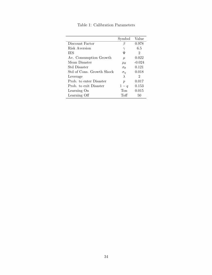
Table 1: Calibration Parameters

Symbol Value

Discount Factor β 0.978Risk Aversion γ 6.5IES Ψ 2Av. Consumption Growth µ 0.022Mean Disaster µθ -0.024Std Disaster σθ 0.121Std of Cons. Growth Shock ση 0.018Leverage λ 2Prob. to enter Disaster p 0.017Prob. to exit Disaster 1− q 0.153Learning On Ton 0.015Learning Off Toff 50

34

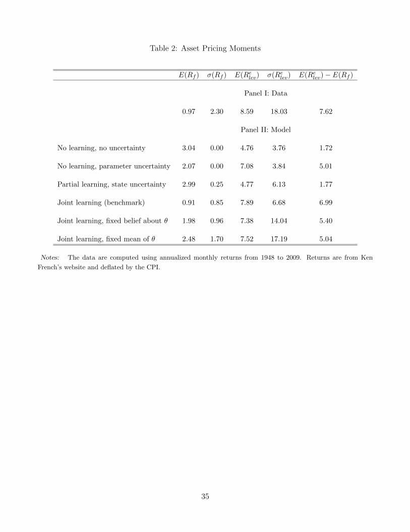
Table 2: Asset Pricing Moments

E(Rf ) σ(Rf ) E(Relev) σ(Relev) E(Relev)− E(Rf )

Panel I: Data

0.97 2.30 8.59 18.03 7.62

Panel II: Model

No learning, no uncertainty 3.04 0.00 4.76 3.76 1.72

No learning, parameter uncertainty 2.07 0.00 7.08 3.84 5.01

Partial learning, state uncertainty 2.99 0.25 4.77 6.13 1.77

Joint learning (benchmark) 0.91 0.85 7.89 6.68 6.99

Joint learning, fixed belief about θ 1.98 0.96 7.38 14.04 5.40

Joint learning, fixed mean of θ 2.48 1.70 7.52 17.19 5.04

Notes: The data are computed using annualized monthly returns from 1948 to 2009. Returns are from Ken

French’s website and deflated by the CPI.

35

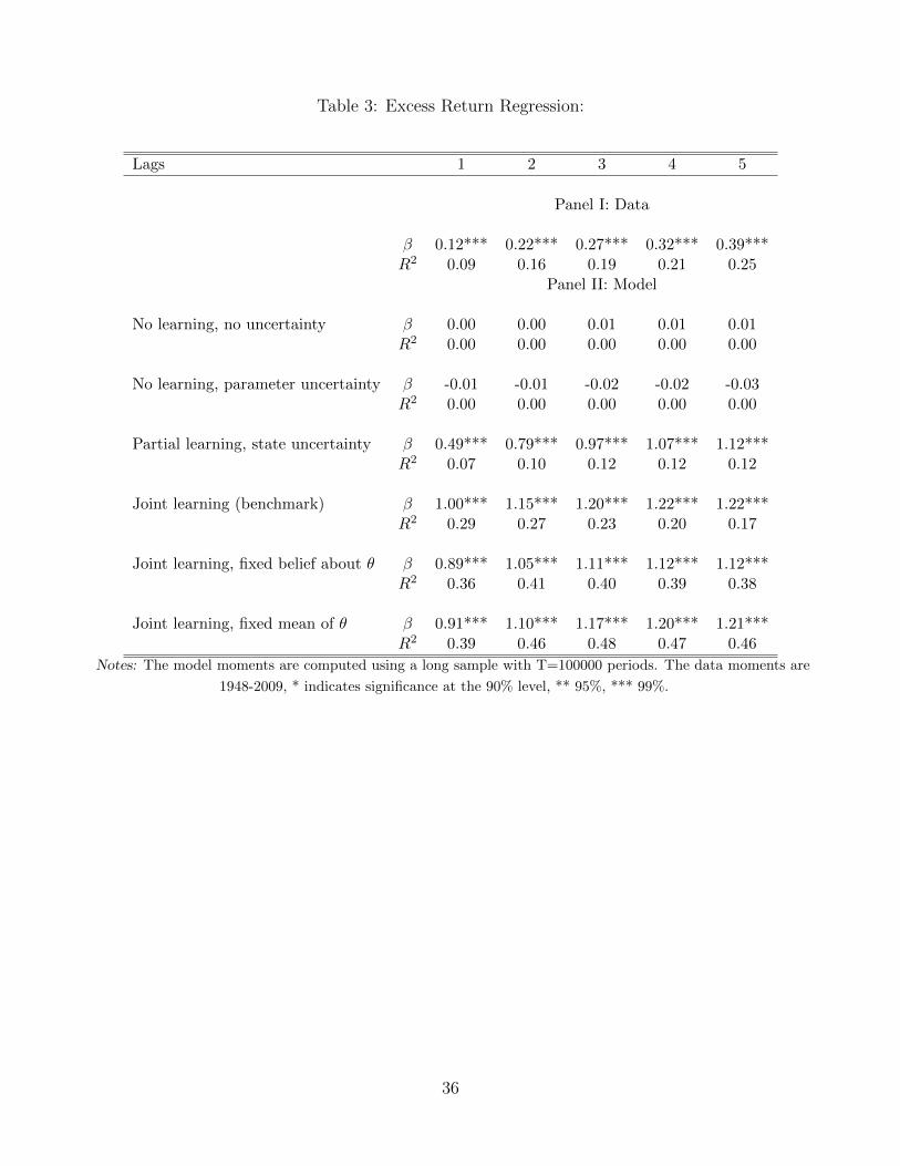
Table 3: Excess Return Regression:

Lags 1 2 3 4 5

Panel I: Data

β 0.12*** 0.22*** 0.27*** 0.32*** 0.39***R2 0.09 0.16 0.19 0.21 0.25

Panel II: Model

No learning, no uncertainty β 0.00 0.00 0.01 0.01 0.01R2 0.00 0.00 0.00 0.00 0.00

No learning, parameter uncertainty β -0.01 -0.01 -0.02 -0.02 -0.03R2 0.00 0.00 0.00 0.00 0.00

Partial learning, state uncertainty β 0.49*** 0.79*** 0.97*** 1.07*** 1.12***R2 0.07 0.10 0.12 0.12 0.12

Joint learning (benchmark) β 1.00*** 1.15*** 1.20*** 1.22*** 1.22***R2 0.29 0.27 0.23 0.20 0.17

Joint learning, fixed belief about θ β 0.89*** 1.05*** 1.11*** 1.12*** 1.12***R2 0.36 0.41 0.40 0.39 0.38

Joint learning, fixed mean of θ β 0.91*** 1.10*** 1.17*** 1.20*** 1.21***R2 0.39 0.46 0.48 0.47 0.46

Notes: The model moments are computed using a long sample with T=100000 periods. The data moments are

1948-2009, * indicates significance at the 90% level, ** 95%, *** 99%.

36

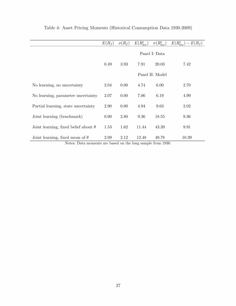
Table 4: Asset Pricing Moments (Historical Consumption Data 1930-2009)


Panel I: Data

0.49 3.93 7.91 20.03 7.42

Panel II: Model







Notes: Data moments are based on the long sample from 1930.

37

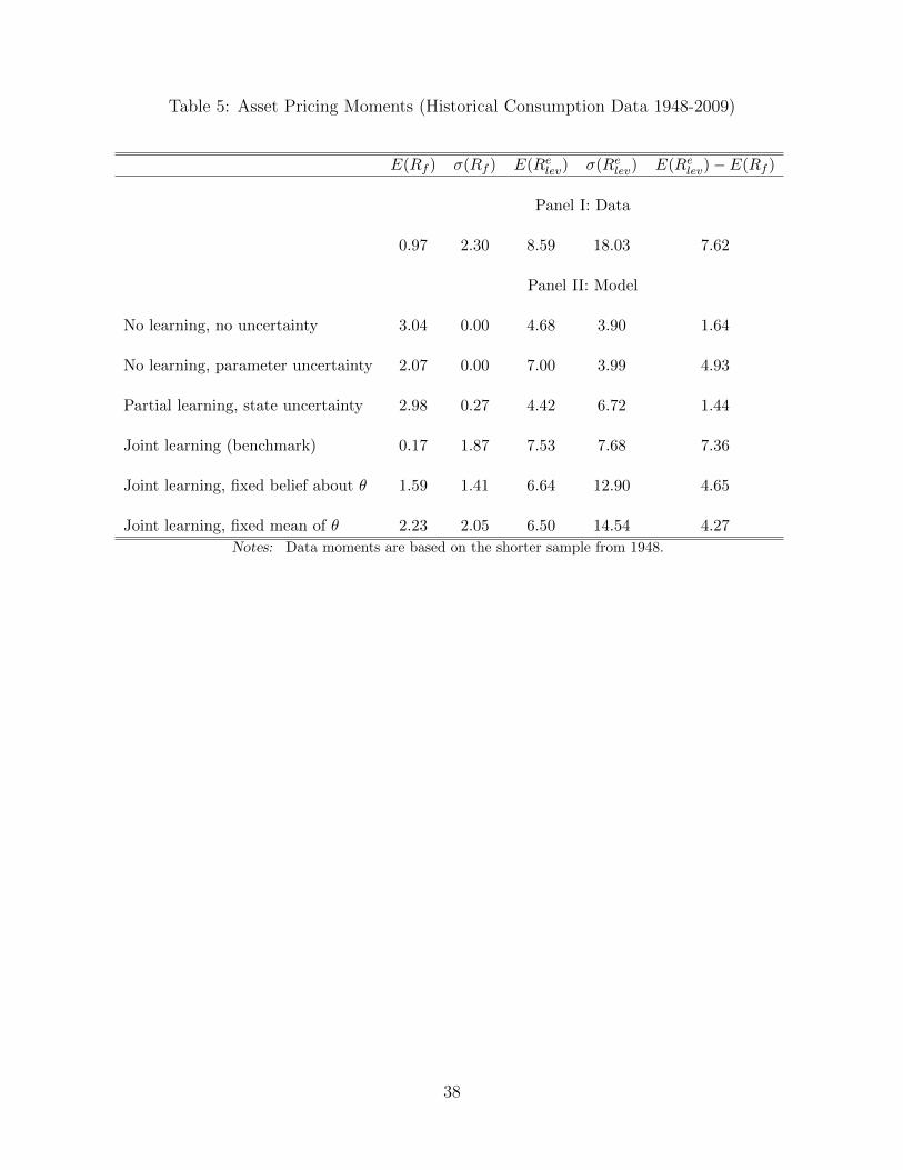
Table 5: Asset Pricing Moments (Historical Consumption Data 1948-2009)


Panel I: Data

0.97 2.30 8.59 18.03 7.62

Panel II: Model







Notes: Data moments are based on the shorter sample from 1948.

38

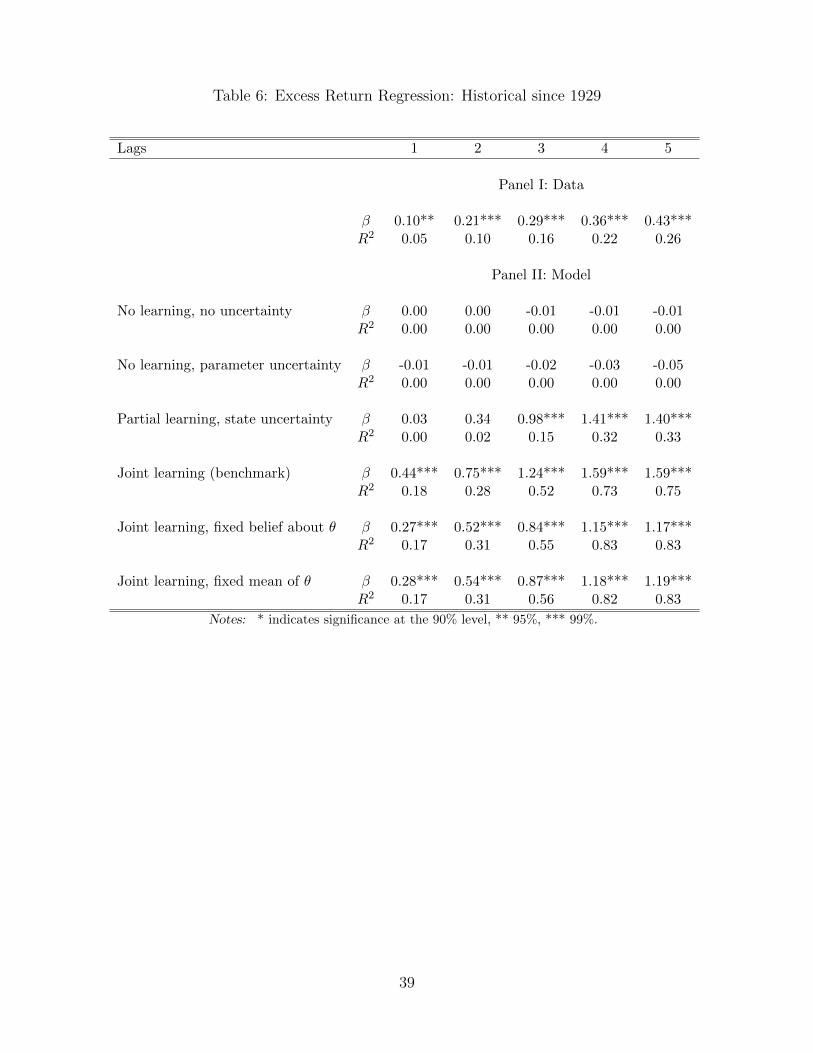
Table 6: Excess Return Regression: Historical since 1929

Lags 1 2 3 4 5

Panel I: Data

β 0.10** 0.21*** 0.29*** 0.36*** 0.43***R2 0.05 0.10 0.16 0.22 0.26

Panel II: Model

No learning, no uncertainty β 0.00 0.00 -0.01 -0.01 -0.01R2 0.00 0.00 0.00 0.00 0.00


Partial learning, state uncertainty β 0.03 0.34 0.98*** 1.41*** 1.40***R2 0.00 0.02 0.15 0.32 0.33

Joint learning (benchmark) β 0.44*** 0.75*** 1.24*** 1.59*** 1.59***R2 0.18 0.28 0.52 0.73 0.75

Joint learning, fixed belief about θ β 0.27*** 0.52*** 0.84*** 1.15*** 1.17***R2 0.17 0.31 0.55 0.83 0.83


Notes: * indicates significance at the 90% level, ** 95%, *** 99%.

39

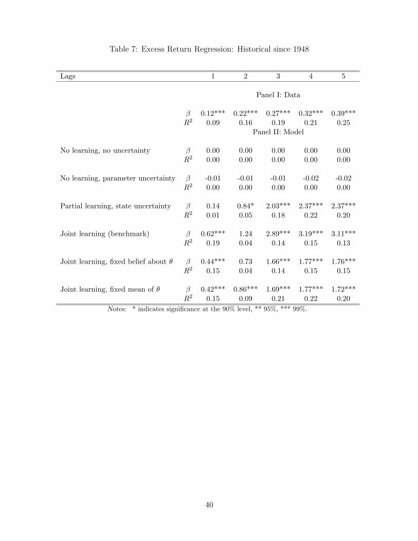
Table 7: Excess Return Regression: Historical since 1948

Lags 1 2 3 4 5

Panel I: Data

β 0.12*** 0.22*** 0.27*** 0.32*** 0.39***R2 0.09 0.16 0.19 0.21 0.25

Panel II: Model

No learning, no uncertainty β 0.00 0.00 0.00 0.00 0.00R2 0.00 0.00 0.00 0.00 0.00


Partial learning, state uncertainty β 0.14 0.84* 2.03*** 2.37*** 2.37***R2 0.01 0.05 0.18 0.22 0.20

Joint learning (benchmark) β 0.62*** 1.24 2.89*** 3.19*** 3.11***R2 0.19 0.04 0.14 0.15 0.13

Joint learning, fixed belief about θ β 0.44*** 0.73 1.66*** 1.77*** 1.76***R2 0.15 0.04 0.14 0.15 0.15


Notes: * indicates significance at the 90% level, ** 95%, *** 99%.

40

2 4 6 8 10 12 14 16 18 20−0.4

−0.2

0

0.2

0.4

0.6

0.8

Disaster Realization

Consumption path

Risk free rate

Levered Equity Return

(a) No learning, no uncertainty

2 4 6 8 10 12 14 16 18 200

0.1

0.2

0.3

0.4

0.5

0.6

0.7

0.8

0.9

1


Belief

(b) No learning, no uncertainty

2 4 6 8 10 12 14 16 18 20−0.4

−0.2

0

0.2

0.4

0.6

0.8


Consumption path

Risk free rate


(c) No learning, parameter uncertainty

2 4 6 8 10 12 14 16 18 200

0.1

0.2

0.3

0.4

0.5

0.6

0.7

0.8

0.9

1


Belief

(d) No learning, parameter uncertainty

2 4 6 8 10 12 14 16 18 20−0.4

−0.2

0

0.2

0.4

0.6

0.8


Consumption path

Risk free rate


(e) Partial learning, state uncertainty

2 4 6 8 10 12 14 16 18 200

0.1

0.2

0.3

0.4

0.5

0.6

0.7

0.8

0.9

1


Belief

(f) Partial learning, state uncertainty

Figure 1: Sample Disaster, Part 1

41

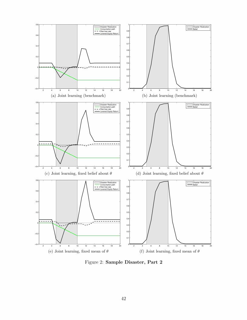
2 4 6 8 10 12 14 16 18 20−0.4

−0.2

0

0.2

0.4

0.6

0.8


Consumption path

Risk free rate


(a) Joint learning (benchmark)

2 4 6 8 10 12 14 16 18 200

0.1

0.2

0.3

0.4

0.5

0.6

0.7

0.8

0.9

1


Belief

(b) Joint learning (benchmark)

2 4 6 8 10 12 14 16 18 20−0.4

−0.2

0

0.2

0.4

0.6

0.8


Consumption path

Risk free rate


(c) Joint learning, fixed belief about θ

2 4 6 8 10 12 14 16 18 200

0.1

0.2

0.3

0.4

0.5

0.6

0.7

0.8

0.9

1


Belief

(d) Joint learning, fixed belief about θ

2 4 6 8 10 12 14 16 18 20−0.4

−0.2

0

0.2

0.4

0.6

0.8


Consumption path

Risk free rate


(e) Joint learning, fixed mean of θ

2 4 6 8 10 12 14 16 18 200

0.1

0.2

0.3

0.4

0.5

0.6

0.7

0.8

0.9

1


Belief

(f) Joint learning, fixed mean of θ

Figure 2: Sample Disaster, Part 2

42

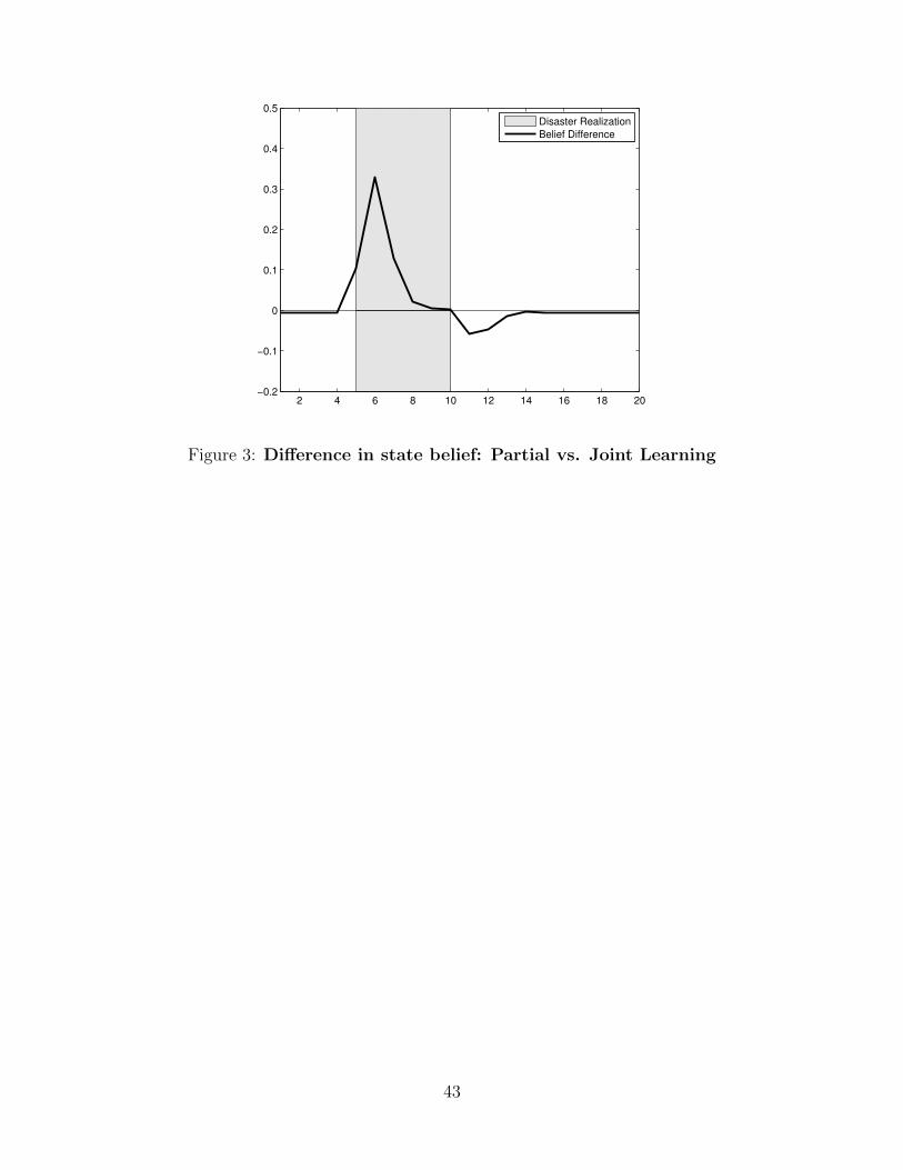
2 4 6 8 10 12 14 16 18 20−0.2

−0.1

0

0.1

0.2

0.3

0.4

0.5


Belief Difference

Figure 3: Difference in state belief: Partial vs. Joint Learning

43

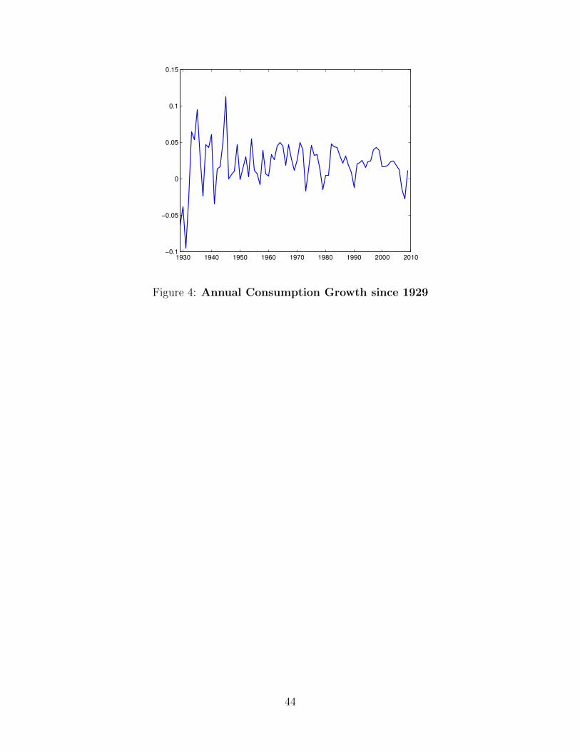
1930 1940 1950 1960 1970 1980 1990 2000 2010−0.1

−0.05

0

0.05

0.1

0.15

Figure 4: Annual Consumption Growth since 1929

44

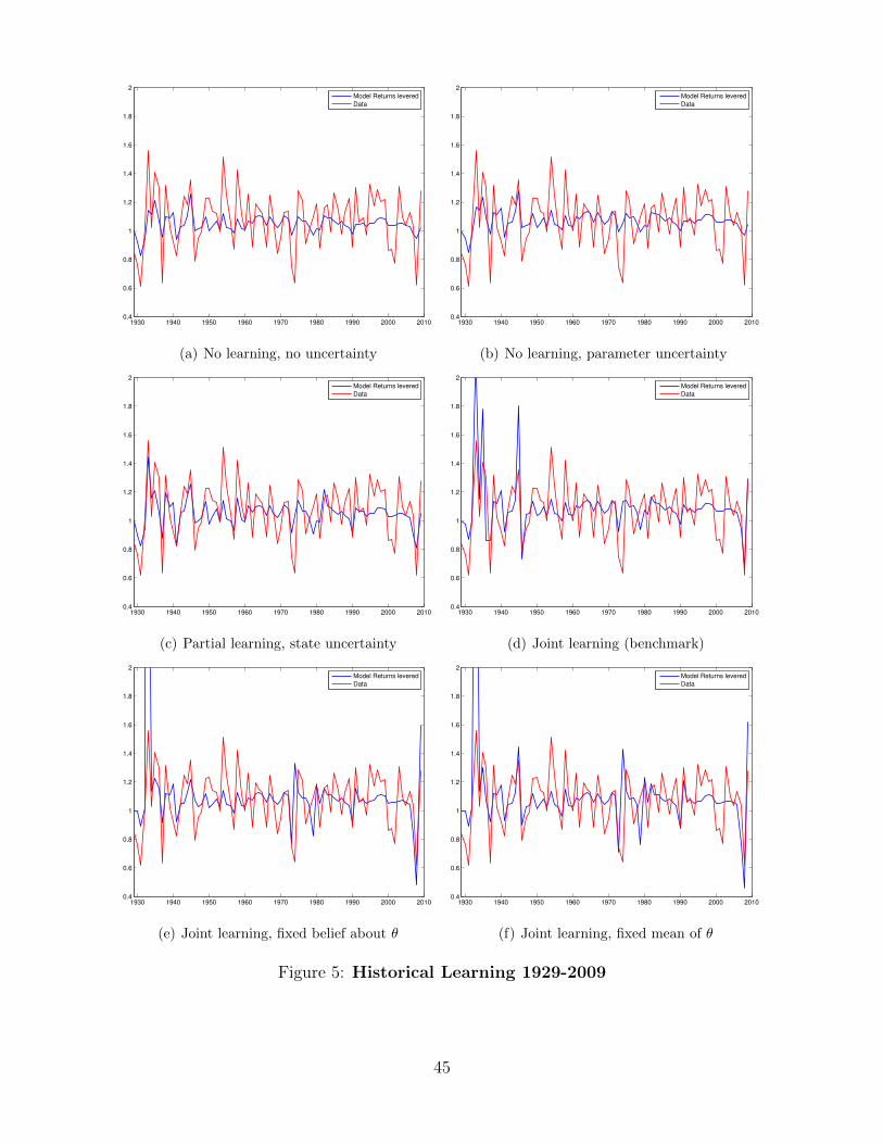
1930 1940 1950 1960 1970 1980 1990 2000 20100.4

0.6

0.8

1

1.2

1.4

1.6

1.8

2

Model Returns levered

Data

(a) No learning, no uncertainty

1930 1940 1950 1960 1970 1980 1990 2000 20100.4

0.6

0.8

1

1.2

1.4

1.6

1.8

2


Data

(b) No learning, parameter uncertainty

1930 1940 1950 1960 1970 1980 1990 2000 20100.4

0.6

0.8

1

1.2

1.4

1.6

1.8

2


Data

(c) Partial learning, state uncertainty

1930 1940 1950 1960 1970 1980 1990 2000 20100.4

0.6

0.8

1

1.2

1.4

1.6

1.8

2


Data

(d) Joint learning (benchmark)

1930 1940 1950 1960 1970 1980 1990 2000 20100.4

0.6

0.8

1

1.2

1.4

1.6

1.8

2


Data

(e) Joint learning, fixed belief about θ

1930 1940 1950 1960 1970 1980 1990 2000 20100.4

0.6

0.8

1

1.2

1.4

1.6

1.8

2


Data

(f) Joint learning, fixed mean of θ

Figure 5: Historical Learning 1929-2009

45

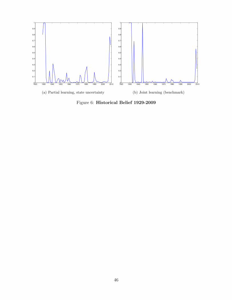
1920 1930 1940 1950 1960 1970 1980 1990 2000 20100

0.1

0.2

0.3

0.4

0.5

0.6

0.7

0.8

0.9

1

(a) Partial learning, state uncertainty

1920 1930 1940 1950 1960 1970 1980 1990 2000 20100

0.1

0.2

0.3

0.4

0.5

0.6

0.7

0.8

0.9

1

(b) Joint learning (benchmark)

Figure 6: Historical Belief 1929-2009

46

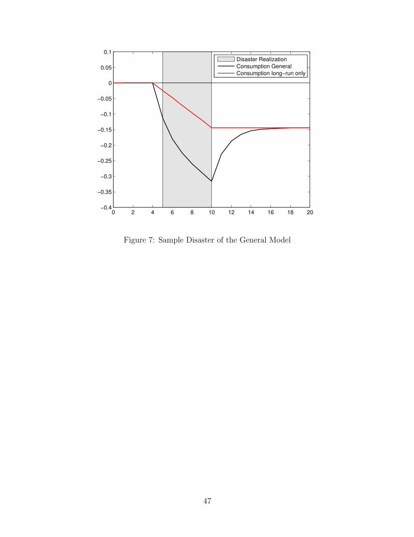
0 2 4 6 8 10 12 14 16 18 20−0.4

−0.35

−0.3

−0.25

−0.2

−0.15

−0.1

−0.05

0

0.05

0.1


Consumption General

Consumption long−run only

Figure 7: Sample Disaster of the General Model

47

Documents

Asset Pricing with Learning about Disaster Risk Yang.pdf · Asset Pricing with Learning about Disaster Risk ... This paper studies asset pricing in an endowment ... where the most