Embed Size (px)
Citation preview

Asset Management
Lecture 10

Table 27.2
Make up a view and replace the one in spreadsheet 27.2. Recalculate the optimal asset allocation and portfolio expected performance.

Table 27.2
Table 1: Bordered Covariance Matrix based on Historical Excess Returnsand Market-Value Weights and Calculation of Baseline Forecasts
Bonds StocksWeights 0.25 0.75
Bonds 0.25 0.006400 0.004080Stocks 0.75 0.004080 0.028900
sumproduct 0.001165 0.017021 Market portfolio variance V(M) = sum(c11:d11) = 0.018186 Coefficient of risk aversion of representative investor = 3 Baseline market portfolio risk premium = A x V(M) = 0.0546
Covariance with RM 0.00466 0.022695
Baseline risk premiums 0.01 0.07
Proportion of covariance attributed to expected returns: 0.01Covariance matrix of expected returns
Bonds StocksBonds 0.000064 0.0000408Stocks 0.0000408 0.000289
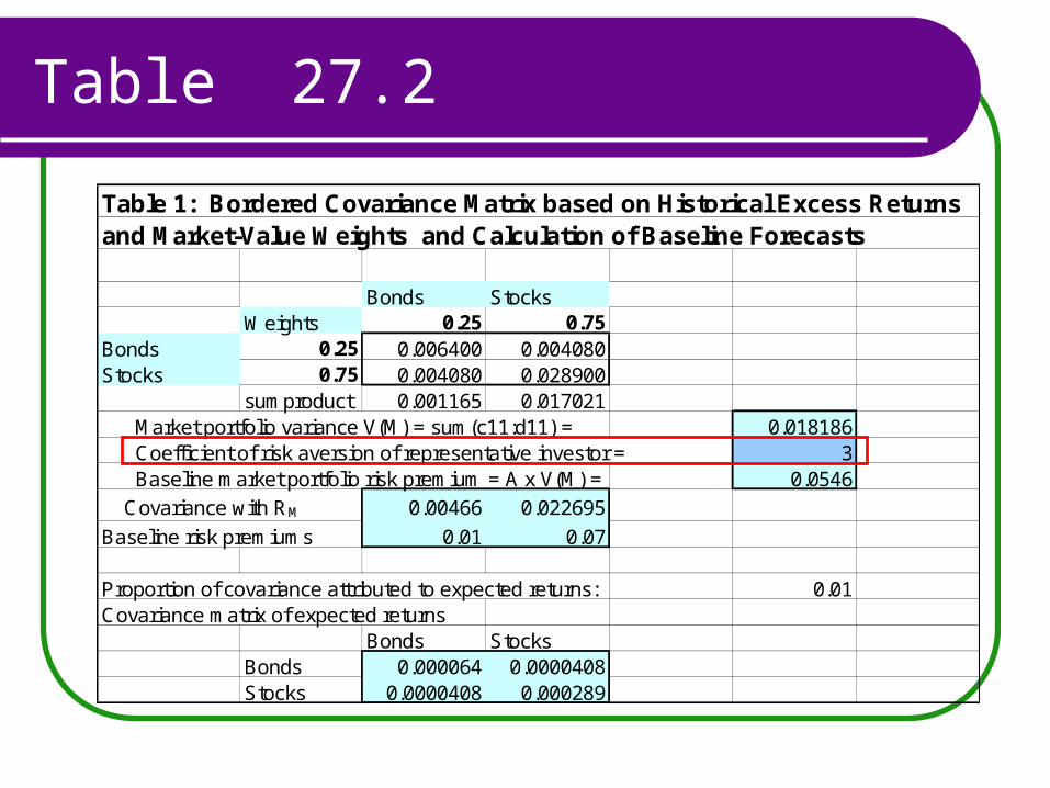

Table 27.2
)()( MM RVarARE
Table 1: Bordered Covariance Matrix based on Historical Excess Returnsand Market-Value Weights and Calculation of Baseline Forecasts
Bonds StocksWeights 0.25 0.75
Bonds 0.25 0.006400 0.004080Stocks 0.75 0.004080 0.028900
sumproduct 0.001165 0.017021 Market portfolio variance V(M) = sum(c11:d11) = 0.018186 Coefficient of risk aversion of representative investor = 3 Baseline market portfolio risk premium = A x V(M) = 0.0546
Covariance with RM 0.00466 0.022695
Baseline risk premiums 0.01 0.07
Proportion of covariance attributed to expected returns: 0.01Covariance matrix of expected returns
Bonds StocksBonds 0.000064 0.0000408Stocks 0.0000408 0.000289

Table 27.2
Table 1: Bordered Covariance Matrix based on Historical Excess Returnsand Market-Value Weights and Calculation of Baseline Forecasts
Bonds StocksWeights 0.25 0.75
Bonds 0.25 0.006400 0.004080Stocks 0.75 0.004080 0.028900
sumproduct 0.001165 0.017021 Market portfolio variance V(M) = sum(c11:d11) = 0.018186 Coefficient of risk aversion of representative investor = 3 Baseline market portfolio risk premium = A x V(M) = 0.0546
Covariance with RM 0.00466 0.022695
Baseline risk premiums 0.01 0.07
Proportion of covariance attributed to expected returns: 0.01Covariance matrix of expected returns
Bonds StocksBonds 0.000064 0.0000408Stocks 0.0000408 0.000289
),()()( , SBSBBMB RRCovwRVarwRRCov

Table 27.2
Table 1: Bordered Covariance Matrix based on Historical Excess Returnsand Market-Value Weights and Calculation of Baseline Forecasts
Bonds StocksWeights 0.25 0.75
Bonds 0.25 0.006400 0.004080Stocks 0.75 0.004080 0.028900
sumproduct 0.001165 0.017021 Market portfolio variance V(M) = sum(c11:d11) = 0.018186 Coefficient of risk aversion of representative investor = 3 Baseline market portfolio risk premium = A x V(M) = 0.0546
Covariance with RM 0.00466 0.022695
Baseline risk premiums 0.01 0.07
Proportion of covariance attributed to expected returns: 0.01Covariance matrix of expected returns
Bonds StocksBonds 0.000064 0.0000408Stocks 0.0000408 0.000289
%40.1%46.5018186.0
00466.0)(
)(
)()( , M
M
MBB RE
RVar
RRCovRE

Table 27.2
Table 1: Bordered Covariance Matrix based on Historical Excess Returnsand Market-Value Weights and Calculation of Baseline Forecasts
Bonds StocksWeights 0.25 0.75
Bonds 0.25 0.006400 0.004080Stocks 0.75 0.004080 0.028900
sumproduct 0.001165 0.017021 Market portfolio variance V(M) = sum(c11:d11) = 0.018186 Coefficient of risk aversion of representative investor = 3 Baseline market portfolio risk premium = A x V(M) = 0.0546
Covariance with RM 0.00466 0.022695
Baseline risk premiums 0.01 0.07
Proportion of covariance attributed to expected returns: 0.01Covariance matrix of expected returns
Bonds StocksBonds 0.000064 0.0000408Stocks 0.0000408 0.000289

Table 27.2
Table 2: Views, Confidence and Revised (Posterior) Expectations
View: Difference between returns on bonds and stocks, Q = 0.0050View embedded in baseline forecasts QE = -0.0541Variance of QE = Var(RB – RS) 0.000271
Var[E(RB)] – Cov[E(RB),E(RS)] = 0.000023
Cov[E(RB),E(RS)] – Var[E(RS)] = -0.000248
Difference between view and baseline data, D = 0.0591Confidence measured by standard deviation of view QPossible SD 0 0.0100 0.0173 0.0300 0.0600Variance 0 0.0015 0.0003 0.0009 0.0036 BaselineE(RB|P) 0.0190 0.0148 0.0164 0.0152 0.0143 0.0140E(RS|P) 0.0140 0.0598 0.0424 0.0556 0.0643 0.0681

Table 27.2
%41.581.640.1'
%)81.6%,40.1())(),((
)1,1(
EE
SBE
PRQ
RERER
P
Table 2: Views, Confidence and Revised (Posterior) Expectations
View: Difference between returns on bonds and stocks, Q = 0.0050View embedded in baseline forecasts QE = -0.0541Variance of QE = Var(RB – RS) 0.000271
Var[E(RB)] – Cov[E(RB),E(RS)] = 0.000023
Cov[E(RB),E(RS)] – Var[E(RS)] = -0.000248
Difference between view and baseline data, D = 0.0591Confidence measured by standard deviation of view QPossible SD 0 0.0100 0.0173 0.0300 0.0600Variance 0 0.0015 0.0003 0.0009 0.0036 BaselineE(RB|P) 0.0190 0.0148 0.0164 0.0152 0.0143 0.0140E(RS|P) 0.0140 0.0598 0.0424 0.0556 0.0643 0.0681

Table 27.2
))()(()(2SB
E REREVarQ ))(),((2)( 2
)(2
)(2
SBREREE RERECovQ
SB
0002714.00000408.02000289.0000064.0)(2 EQ
Table 2: Views, Confidence and Revised (Posterior) Expectations
View: Difference between returns on bonds and stocks, Q = 0.0050View embedded in baseline forecasts QE = -0.0541Variance of QE = Var(RB – RS) 0.000271
Var[E(RB)] – Cov[E(RB),E(RS)] = 0.000023
Cov[E(RB),E(RS)] – Var[E(RS)] = -0.000248
Difference between view and baseline data, D = 0.0591Confidence measured by standard deviation of view QPossible SD 0 0.0100 0.0173 0.0300 0.0600Variance 0 0.0015 0.0003 0.0009 0.0036 BaselineE(RB|P) 0.0190 0.0148 0.0164 0.0152 0.0143 0.0140E(RS|P) 0.0140 0.0598 0.0424 0.0556 0.0643 0.0681

Table 27.2
Table 2: Views, Confidence and Revised (Posterior) Expectations
View: Difference between returns on bonds and stocks, Q = 0.0050View embedded in baseline forecasts QE = -0.0541Variance of QE = Var(RB – RS) 0.000271
Var[E(RB)] – Cov[E(RB),E(RS)] = 0.000023
Cov[E(RB),E(RS)] – Var[E(RS)] = -0.000248
Difference between view and baseline data, D = 0.0591Confidence measured by standard deviation of view QPossible SD 0 0.0100 0.0173 0.0300 0.0600Variance 0 0.0015 0.0003 0.0009 0.0036 BaselineE(RB|P) 0.0190 0.0148 0.0164 0.0152 0.0143 0.0140E(RS|P) 0.0140 0.0598 0.0424 0.0556 0.0643 0.0681
2
2)( )(),(
)|(D
SBREBB
RERECovDREPRE B

Table 27.2
Table 1: Bordered Covariance Matrix based on Historical Excess Returnsand Market-Value Weights and Calculation of Baseline Forecasts
Bonds StocksWeights 0.25 0.75
Bonds 0.25 0.006400 0.004080Stocks 0.75 0.004080 0.028900
sumproduct 0.001165 0.017021 Market portfolio variance V(M) = sum(c11:d11) = 0.018186 Coefficient of risk aversion of representative investor = 3 Baseline market portfolio risk premium = A x V(M) = 0.0546
Covariance with RM 0.00466 0.022695
Baseline risk premiums 0.01 0.07
Proportion of covariance attributed to expected returns: 0.01Covariance matrix of expected returns
Bonds StocksBonds 0.000064 0.0000408Stocks 0.0000408 0.000289
%40.1%46.5018186.0
00466.0)(
)(
)()( , M
M
MBB RE
RVar
RRCovRE

Table 27.2
Table 2: Views, Confidence and Revised (Posterior) Expectations
View: Difference between returns on bonds and stocks, Q = 0.0050View embedded in baseline forecasts QE = -0.0541Variance of QE = Var(RB – RS) 0.000271
Var[E(RB)] – Cov[E(RB),E(RS)] = 0.000023
Cov[E(RB),E(RS)] – Var[E(RS)] = -0.000248
Difference between view and baseline data, D = 0.0591Confidence measured by standard deviation of view QPossible SD 0 0.0100 0.0173 0.0300 0.0600Variance 0 0.0015 0.0003 0.0009 0.0036 BaselineE(RB|P) 0.0190 0.0148 0.0164 0.0152 0.0143 0.0140E(RS|P) 0.0140 0.0598 0.0424 0.0556 0.0643 0.0681
2
2)( )(),(
)|(D
SBREBB
RERECovDREPRE B

Table 27.2
Table 1: Bordered Covariance Matrix based on Historical Excess Returnsand Market-Value Weights and Calculation of Baseline Forecasts
Bonds StocksWeights 0.25 0.75
Bonds 0.25 0.006400 0.004080Stocks 0.75 0.004080 0.028900
sumproduct 0.001165 0.017021 Market portfolio variance V(M) = sum(c11:d11) = 0.018186 Coefficient of risk aversion of representative investor = 3 Baseline market portfolio risk premium = A x V(M) = 0.0546
Covariance with RM 0.00466 0.022695
Baseline risk premiums 0.01 0.07
Proportion of covariance attributed to expected returns: 0.01Covariance matrix of expected returns
Bonds StocksBonds 0.000064 0.0000408Stocks 0.0000408 0.000289
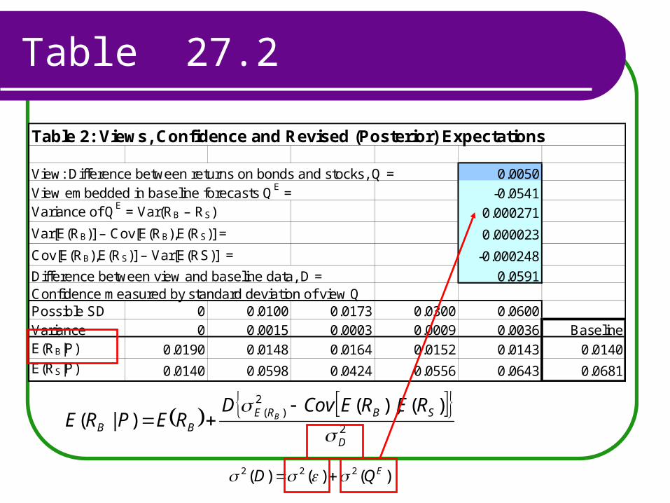
Table 27.2
2
2)( )(),(
)|(D
SBREBB
RERECovDREPRE B
Table 2: Views, Confidence and Revised (Posterior) Expectations
View: Difference between returns on bonds and stocks, Q = 0.0050View embedded in baseline forecasts QE = -0.0541Variance of QE = Var(RB – RS) 0.000271
Var[E(RB)] – Cov[E(RB),E(RS)] = 0.000023
Cov[E(RB),E(RS)] – Var[E(RS)] = -0.000248
Difference between view and baseline data, D = 0.0591Confidence measured by standard deviation of view QPossible SD 0 0.0100 0.0173 0.0300 0.0600Variance 0 0.0015 0.0003 0.0009 0.0036 BaselineE(RB|P) 0.0190 0.0148 0.0164 0.0152 0.0143 0.0140E(RS|P) 0.0140 0.0598 0.0424 0.0556 0.0643 0.0681
)()()( 222 EQD

Table 27.2
)()()( 222 EQD
Table 2: Views, Confidence and Revised (Posterior) Expectations
View: Difference between returns on bonds and stocks, Q = 0.0050View embedded in baseline forecasts QE = -0.0541Variance of QE = Var(RB – RS) 0.000271
Var[E(RB)] – Cov[E(RB),E(RS)] = 0.000023
Cov[E(RB),E(RS)] – Var[E(RS)] = -0.000248
Difference between view and baseline data, D = 0.0591Confidence measured by standard deviation of view QPossible SD 0 0.0100 0.0173 0.0300 0.0600Variance 0 0.0015 0.0003 0.0009 0.0036 BaselineE(RB|P) 0.0190 0.0148 0.0164 0.0152 0.0143 0.0140E(RS|P) 0.0140 0.0598 0.0424 0.0556 0.0643 0.0681
)()()( 10 ttaaatu f

Table 27.2
Table 2: Views, Confidence and Revised (Posterior) Expectations
View: Difference between returns on bonds and stocks, Q = 0.0050View embedded in baseline forecasts QE = -0.0541Variance of QE = Var(RB – RS) 0.000271
Var[E(RB)] – Cov[E(RB),E(RS)] = 0.000023
Cov[E(RB),E(RS)] – Var[E(RS)] = -0.000248
Difference between view and baseline data, D = 0.0591Confidence measured by standard deviation of view QPossible SD 0 0.0100 0.0173 0.0300 0.0600Variance 0 0.0015 0.0003 0.0009 0.0036 BaselineE(RB|P) 0.0190 0.0148 0.0164 0.0152 0.0143 0.0140E(RS|P) 0.0140 0.0598 0.0424 0.0556 0.0643 0.0681
2
2)()(),(
)|(D
RESBSS
SRERECovD
REPRE
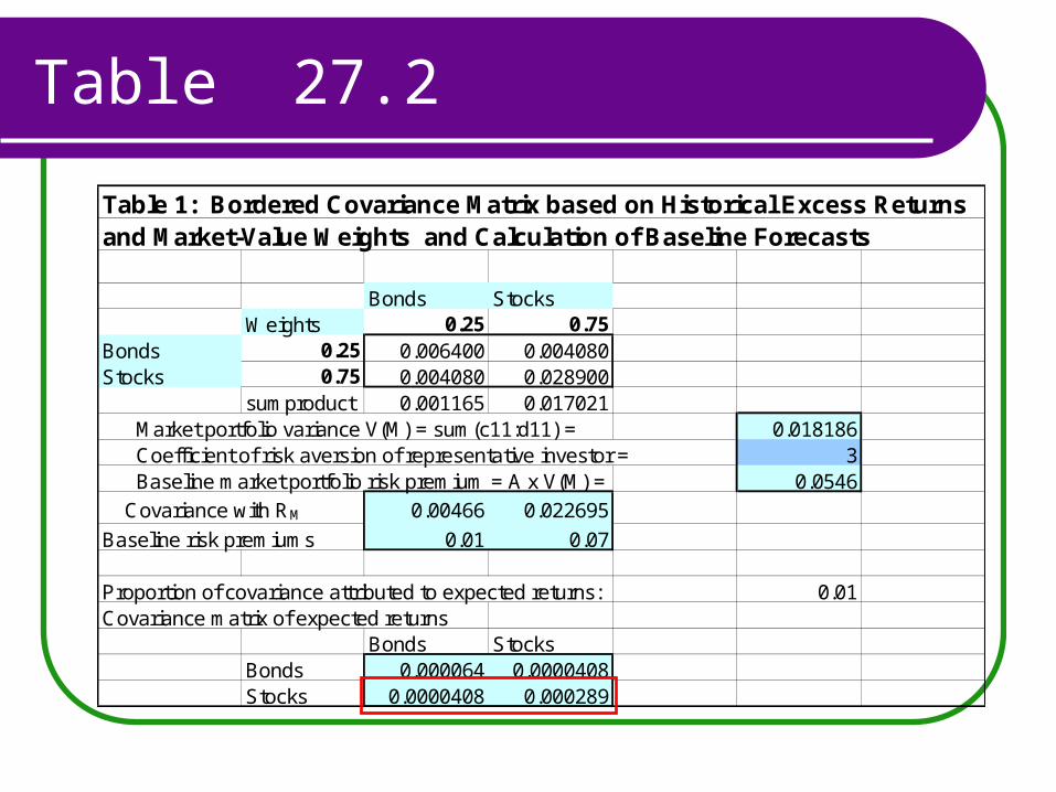
Table 27.2
Table 1: Bordered Covariance Matrix based on Historical Excess Returnsand Market-Value Weights and Calculation of Baseline Forecasts
Bonds StocksWeights 0.25 0.75
Bonds 0.25 0.006400 0.004080Stocks 0.75 0.004080 0.028900
sumproduct 0.001165 0.017021 Market portfolio variance V(M) = sum(c11:d11) = 0.018186 Coefficient of risk aversion of representative investor = 3 Baseline market portfolio risk premium = A x V(M) = 0.0546
Covariance with RM 0.00466 0.022695
Baseline risk premiums 0.01 0.07
Proportion of covariance attributed to expected returns: 0.01Covariance matrix of expected returns
Bonds StocksBonds 0.000064 0.0000408Stocks 0.0000408 0.000289

Table 27.2
Table 2: Views, Confidence and Revised (Posterior) Expectations
View: Difference between returns on bonds and stocks, Q = 0.0050View embedded in baseline forecasts QE = -0.0541Variance of QE = Var(RB – RS) 0.000271
Var[E(RB)] – Cov[E(RB),E(RS)] = 0.000023
Cov[E(RB),E(RS)] – Var[E(RS)] = -0.000248
Difference between view and baseline data, D = 0.0591Confidence measured by standard deviation of view QPossible SD 0 0.0100 0.0173 0.0300 0.0600Variance 0 0.0015 0.0003 0.0009 0.0036 BaselineE(RB|P) 0.0190 0.0148 0.0164 0.0152 0.0143 0.0140E(RS|P) 0.0140 0.0598 0.0424 0.0556 0.0643 0.0681

Exercise 27.4
Make up a view and replace the one in spreadsheet 27.2. Recalculate the optimal asset allocation and portfolio expected performance.

Exercise 27.3
Make up new alpha forecasts for your portfolio from Assignment One. Use Traynor Black model to find the optimal portfolio.
The assignment is due on April 14.