Asset Localization in Data Centers using WUSBRadios

N. Udar†, K. Kant‡, R. Viswanathan†?

Abstract. Asset tracking is a critical problem in modern data centerswith modular and easily movable servers. This paper studies a wirelessasset tracking solution built using wireless USB (WUSB) radios that areexpected to ubiquitous in future servers. This paper builds on our pre-vious work on direct ranging using WUSB radios and studies algorithmsfor data center wide localization of all rack mounted servers. The resultsshow that it is possible achieve very low error rates in localization inspite of very stringent constraints (i.e., each server being just 1.8” high)by exploiting the properties of the data center environment.

Key words: Ultra Wideband (UWB), Wireless USB, data centers, channelmodel, localization, Maximum Likelihood Estimation

1 Introduction

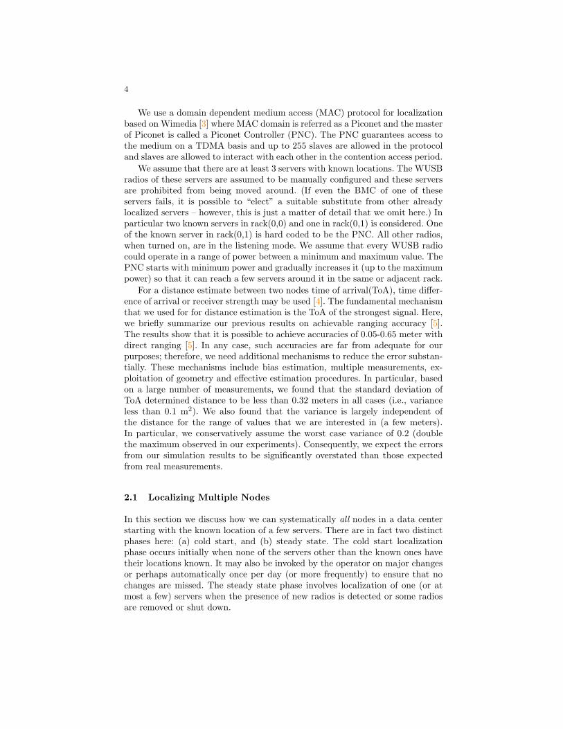
Data centers form the backbone of modern commerce and continue to grow bothin terms of number of servers and number of servers per unit volume of datacenter space. Modern data centers sport rows upon rows of “racks”, each withcertain number of standard size “slots” where various “assets” (servers, routers,switches, storage bricks, etc.) can be inserted. Fig. 1 shows a typical row of adata center. Tracking these assets has repeatedly been cited as among the top 5issues facing IT administrators in large data centers and other IT environments.As assets become easier to move – by virtue of smaller sizes, modular struc-ture, hot plug-in/plug-out capabilities – they indeed tend to change locationsmore frequently. There are several reasons for assets to move around: (a) re-placement of old/problematic equipment and/or addition of new equipment andresulting reorganization, (b) manual reorganization of assets to handle evolvingneeds and applications, (c) reorganization driven by power and thermal issueswhich keep becoming more and more severe, (d) removal followed by reinser-tion for miscellaneous reasons including SW patching, etc. One whole, the assetsdon’t necessarily move very much, but in a large data center, even a limitedmovement could become very cumbersome to manage manually. In particular,trivial solutions such as those requiring personnel to log each moved asset in aspreadsheet/database have not worked well in the past. Several vendors includ-ing Sun and HP have devised new solutions, which points to the importance ofthe problem.? †N. Udar and, R. Viswanathan are with Southern Illinois University, Carbondale,

IL. ‡K. Kant is with Intel Corporation, Hillsboro, OR

2

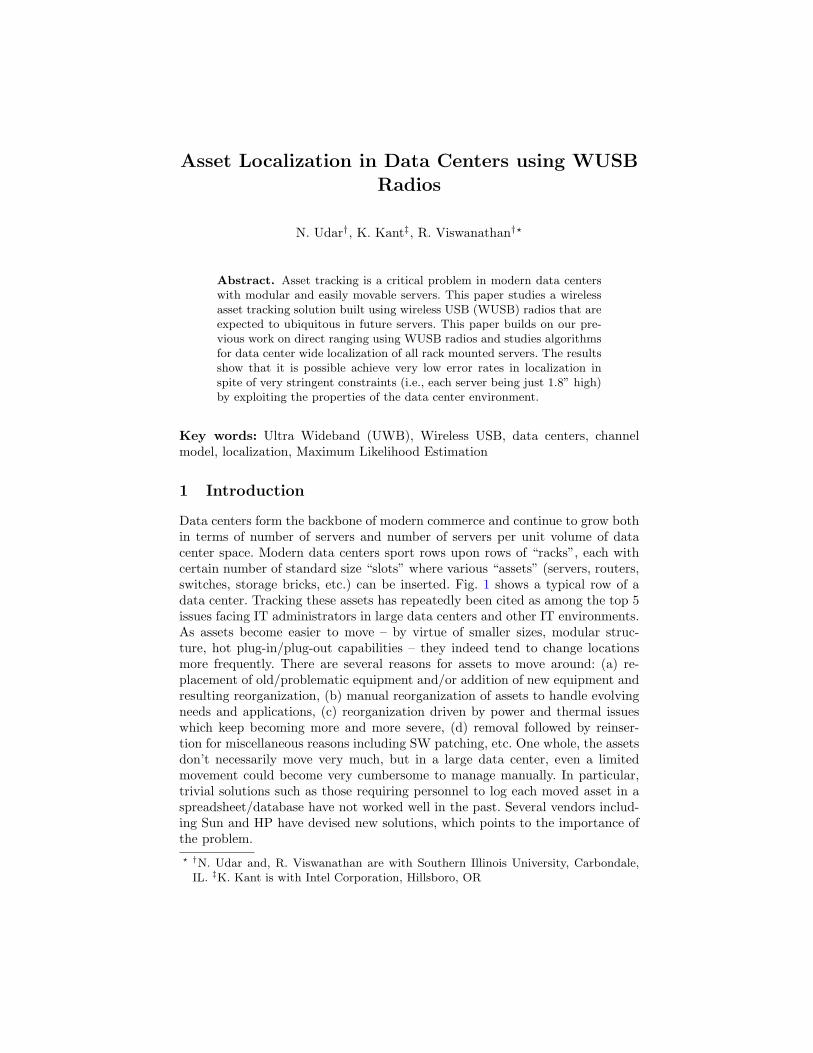
Fig. 1. Racks in a data center Fig. 2. Schematic Rack Layout

From the survey paper [1] on indoor positioning techniques, it can be con-cluded that techniques based on wireless local area network (WLAN) are perhapsreasonable to locate racks in the data center, but too crude for locating servers.Techniques based on surface acoustic wave (SAW) can provide good accuracybut would require a network of SAW sensors to be deployed and managed. Ultrawideband (UWB) based solutions can provide good accuracy, but any externalinfrastructure would add to cost and management issues. In this paper, a wirelessuniversal serial bus(WUSB) based solution is exploited that uses UWB radiosintegrated into the server and does not rely on any external infrastructure. HPhas developed a solution based on an array of passive RFID tags attached toeach server [2]. The solution requires one radio frequency identification (RFID)reader per server which communicates with the rack level data collector. EachRFID reader has a directional antenna mounted on a motorized rack and eachrack has a sensor controller aware of its position. Although an accuracy exceed-ing 98% is claimed for this system, the complexity and cost of the system areexpected to be prohibitive.

In this paper we explore an automated asset tracking solution by exploitingthe WUSB that is expected to replace wired USB in the near future. The basicassumption is that WUSB radios will be integrated with various assets andcould form a sort of mesh fabric which can be exploited for a variety of low-bandwidth applications including asset tracking. There are many reasons whysuch an approach is attractive:

1. WUSB uses UWB radio as its physical layer which is known to have excellentlocalization properties.

2. Given its role as a wired USB replacement, WUSB radio cost should comedown rapidly, which makes the solution inexpensive.

3. Since WUSB radios are assumed to be integrated in each server, such a solu-tion does not require any external infrastructure. Additional infrastructureis usually highly undesirable from an IT personnel’s perspective.

In this paper we focus on “plugged-in” assets that have our integrated solu-tion implemented. The assets don’t necessarily have to be “booted up” or evenpowered, just plugged in. To allow for this, we propose to implement asset local-

3

ization in a server’s baseboard management controller (BMC), which is supposedto be always operational irrespective of the state of the server.

The most challenging aspect of the data center localization problem is theneed for very high accuracy localization. The typical “one meter” accuraciesthat localization methods can typically achieve with significant effort are about 2orders of magnitude worse than what we need in this application. Furthermore,we would like to do this without any additional infrastructure. The outline ofthe paper is as follows. In section 2, we present the configuration of modern datacenters and discuss how a wireless USB based scheme can walk through the entiredata center and localize individual plugged in assets. In section 3 we propose themethod of maximum likelihood identification (MLI) for localization of serversand show that the performance of proposed method far exceeds the performanceof traditional hyperbolic positioning (HBP). The novelty of the MLI solution isthe exploitation of geometric properties of the data center environment to obtainhigh accuracy localization. The performance of MLI is analyzed in section 4. Thesimulation results show that it is possible to achieve good accuracy in a datacenter environment using MLI. Section 5 concludes the discussion.

2 Configuration and Assumptions

The geometric aspects of server arrangement in a data center are crucial to oursolution; hence are described briefly here. The racks, as shown in Fig. 1 are 78”high, 23-25” wide and 26-30” deep and are arranged in rows. The rack rows arearranged in pairs so that the servers in successive odd-even row pairs face oneanother. This creates alternating hot and cold aisles (backs and fronts of servers)and helps make cooling more efficient. The width of these hot and cold aislesis generally different and needs to be accounted for. Fig. 2 shows a simplifiedtop view of this arrangement where the wider aisles are the cold aisles (fronts ofservers). The Fig. 2 also establishes a coordinate system that we will be using inour analysis. The x -axis denotes the row index and the y-axis denotes the rackposition in the row. The z -axis (not shown in the figure) is along the height ofthe rack. For example,(0, 1, 1) denotes that the server is in row 0, rack 1 and atposition 1 in the rack. The positions in the rack are labeled as 1, 2, ..N startingfrom top of the rack.

In this paper, we focus on the popular “rack mount” servers that go directlyinto the racks as shown in Fig. 1. Obviously, the server thickness decides howmany servers can fit in a rack. The standard measure of thickness is “U” (about1.8”). Consequently, a single rack can take up to 42 1U “assets”. The increasinglypopular “Blade servers” go vertically in chassis that in turn fit into racks will beaddressed in future work.

It is assumed that each plugged asset has an integrated WUSB radio accessi-ble from the management controller in the pre boot or post boot environments.We assume that each rack has at least 2 plugged in servers and the racks arearranged in a rectangular pattern – localization with geometries other than arectangle is beyond the scope of the current paper.

4

We use a domain dependent medium access (MAC) protocol for localizationbased on Wimedia [3] where MAC domain is referred as a Piconet and the masterof Piconet is called a Piconet Controller (PNC). The PNC guarantees access tothe medium on a TDMA basis and up to 255 slaves are allowed in the protocoland slaves are allowed to interact with each other in the contention access period.

We assume that there are at least 3 servers with known locations. The WUSBradios of these servers are assumed to be manually configured and these serversare prohibited from being moved around. (If even the BMC of one of theseservers fails, it is possible to “elect” a suitable substitute from other alreadylocalized servers – however, this is just a matter of detail that we omit here.) Inparticular two known servers in rack(0,0) and one in rack(0,1) is considered. Oneof the known server in rack(0,1) is hard coded to be the PNC. All other radios,when turned on, are in the listening mode. We assume that every WUSB radiocould operate in a range of power between a minimum and maximum value. ThePNC starts with minimum power and gradually increases it (up to the maximumpower) so that it can reach a few servers around it in the same or adjacent rack.

For a distance estimate between two nodes time of arrival(ToA), time differ-ence of arrival or receiver strength may be used [4]. The fundamental mechanismthat we used for for distance estimation is the ToA of the strongest signal. Here,we briefly summarize our previous results on achievable ranging accuracy [5].The results show that it is possible to achieve accuracies of 0.05-0.65 meter withdirect ranging [5]. In any case, such accuracies are far from adequate for ourpurposes; therefore, we need additional mechanisms to reduce the error substan-tially. These mechanisms include bias estimation, multiple measurements, ex-ploitation of geometry and effective estimation procedures. In particular, basedon a large number of measurements, we found that the standard deviation ofToA determined distance to be less than 0.32 meters in all cases (i.e., varianceless than 0.1 m2). We also found that the variance is largely independent ofthe distance for the range of values that we are interested in (a few meters).In particular, we conservatively assume the worst case variance of 0.2 (doublethe maximum observed in our experiments). Consequently, we expect the errorsfrom our simulation results to be significantly overstated than those expectedfrom real measurements.

2.1 Localizing Multiple Nodes

In this section we discuss how we can systematically all nodes in a data centerstarting with the known location of a few servers. There are in fact two distinctphases here: (a) cold start, and (b) steady state. The cold start localizationphase occurs initially when none of the servers other than the known ones havetheir locations known. It may also be invoked by the operator on major changesor perhaps automatically once per day (or more frequently) to ensure that nochanges are missed. The steady state phase involves localization of one (or atmost a few) servers when the presence of new radios is detected or some radiosare removed or shut down.

5

The cold-start localization starts with localization of unknown servers inrack (0,0). For rack (0,0) localization, two servers at known locations (knownservers) in rack (0,0) and one known server in rack (0,1) is used as referencenodes. During rack(0,0) localization, all the unknown nodes in rack(0,0) andone unknown node in rack(0,1) and 2 unknown nodes in rack(1,1) are localized.These unknown nodes are then used as reference nodes for corresponding racklocalization. Rack(0,1) onwards during localization 2 reference nodes from thecurrent rack and one reference node from the previous rack. Rack(0,1) localiza-tion onwards exactly 2 nodes in the next rack and 2 nodes in the opposite rackare localized. Thus the row 0 localization is complete. The odd numbered racksneed not localize the servers in the next rack except the ones present in thebeginning of the first rack. For example, rack(1,1) uses two reference nodes fromits rack and one from rack(0,0) and localizes one server in rack(2,0). Thus, allthe servers in the data center are localized from right to left one row at a time.

Each server maintains a local grid map of its neighbors. Local grid map refersto the map of position of neighbors. As the localization is performed, each serverupdates its map to indicate which neighbors are plugged-in.

A critical element in cold-start localization is the avoidance of servers in racksthat we are currently not interested in localizing. The fundamental assumptionin the approach above is that the transmit power is chosen low enough so that thesignal does not reach across more than one rack in either direction. Obviously,this cannot be guaranteed by power control alone. Instead, we need to examineeach distance estimate and determine whether the responder is more than onerack away. That is, the problem requires doing “macro localization” in order toenable systematic localization discussed above. This is another place where wetake advantage of the regular geometry of the racks. Since the rack dimensionsare known and the racks are regularly placed, macro-localization is relativelystraightforward. In particular, if we have 3 known nodes and distances fromthem to an unknown node, simple geometric calculations can easily tell us withhigh probability which rack the unknown node belongs to. In cases where thereis ambiguity, multiple measurements can be used for disambiguation much in thesame way as discussed in section 4.2 for correctly locating new set of referencenodes. For brevity, we omit the details of this procedure.

Once the cold start localization is finished, monitoring in steady state isrelatively simple because several Piconets operating simultaneously monitor theirsurrounding nodes in order to update any changes in the locations of the nodes.

3 Localization Methods

In this section, we consider the issue of accurately estimating the position of asingle unknown node based on distance measurements from a number of knownnodes. We propose the maximum likelihood identification method and comparewith the traditional hyperbolic positioning method.

6

3.1 Hyperbolic Positioning

Hyperbolic Positioning technique requires common time reference only betweenreference nodes and does not rely on the synchronization between referencesnodes and the target node [6]. The position of the target node is determinedbased on the time difference of arrival from two reference nodes. Let us determinethe 2-D position of the target node T (x0, y0) using k reference nodes. Each ofthe reference node makes the range measurement based on TOA with the targetnode denoted as D1T , D2T ....DkT . Let us assume that the reference node sharea common time reference and the clock at the target node T is delayed by δ.Then it is observed that the difference of range measurements between any pairof node removes the delay. The range measurement between any two nodes isgiven as

DkT −DlT = c(τkT + δ)− c(τlT + δ) (1)

where τkT denotes the TOA measured by reference node k from the targetnode. The position of target node T in the 2-D space is determined by theintersection of hyperbola using 3 reference nodes. However, when range mea-surements incur errors due to multi path and noise HBP could show large errorsin localization [7]. In fact, for our problem ML identification shows much betteraccuracies than HBP localization, as will be shown in section 4.

3.2 Maximum Likelihood Identification

Maximum likelihood (ML) testing is a well-known technique for deciding onwhich one of the hypothesized models a measurement came from. Since in ourproblem, we only have 42 discrete possible positions for a server in a rack, themaximum likelihood identification (MLI) deals with identifying which one of theseveral discrete positions is the correct one. For a more formal description ofMLI, consider two nodes at the known locations in rack 1 and one in rack 2 (thiscan be easily extended to p transmitters). Each of the known nodes measurethe distances using TOA from an unknown node at (m, l, n) where m denotesthe row number, m ∈ (0, 1..M), l denotes the rack number l ∈ (0, 1, ..L), and ndenotes the position of the node in the rack, n ∈ (0, 1, 2...N − 1).

Let V out of N -2 (N -2 possible unknown positions for rack 1 ) possiblepositions are filled by plugged-in servers. Each of the V nodes determines itsposition based on its range estimates from the three known nodes.

Let us consider the detection of the location of one of these V nodes say,node u. Since the location of node u is unknown , it hypothesizes its location tobe any one of the possible locations and forms N−2 likelihood functions, one foreach hypothesis, based on the range measurements (r1u, r2u, r3u). For formingthe likelihood function, we assume that a range estimate riu is distributed asGaussian with zero bias (that is, mean equal to the true distance between thereference node i and the node u, diu ) and variance σ2 = N0/2. This model as-sumes line of sight propagation, which may be reasonable when the transmittersand the receivers are in close proximity of each other. In future work we relax

7

this assumption and introduce bias in the range estimates. The node u estimatesits location based on the maximum likelihood rule, i.e., decide location (m, l, n̂),

(m, l, n̂) = argn max p (r1u, r2u, r3u|Hn) (2)

where the row index m is assumed to be correct as we localize one row at a timeand the rack index l is decided based on the geometry of the racks and the threerange estimates as mentioned in section 2.1. Hence, MLI searches only over therack index n.

Since each plugged in server is classified as occupying one of the allowed serverpositions, several types of errors could happen. A server could be misclassifiedto be occupying a wrong position where (i) there actually exists another serveror (ii) there exists no server. Another situation occurs when two or more nodesclaim the same location. This situation could be resolved by subsequent rangemeasurements. For the proposed location estimation system to be successful,it is imperative that the probability of error in the classification of a node isextremely small, especially because the estimation of nodes occurs in successivestages, relying on previous estimates, one rack at a time and one row at a time.We briefly mention the calculation of probability of correctly identifying a nodelocation for the maximum likelihood rule. By expanding eq. 2 and by throwingout the terms that do not depend on n, the equivalent rule picks the maximumof Zn,u = 〈ru,dn〉 − En/2, where ru = (r1u, r2u, r3u)T , dn = (d1n, d2n, d3n)

Here, 〈−,−〉 denotes the inner product between two vectors and En =〈dn,dn〉. Given that the true location of unknown node say, (m,l,u), the prob-ability of correct classification is the probability that Zu,u is the largest amongall possible Zn,u , Finally, a closed expression for error probabilities is similar tocalculating the error probabilities, in the detection of M-ary signals in additivewhite Gaussian noise with arbitrary signal set [8]. It is well-known that the exacterror probability is difficult to calculate but tight upper and lower bounds canbe obtained.

Notice that the maximum likelihood rule does not require the knowledge ofthe variance, as long as the variance is the same for any estimated range. Ifthe variances of the range estimates depend on the distance, then the maximumlikelihood rule would require the values of these variances. However, for shortdistances, spanning the height of a rack or an adjacent rack, a single varianceassumption may be valid as a first approximation [5]. For assessing the effec-tiveness of the algorithm we will use MATLAB simulations and union bounddiscussed in section 3.3.

3.3 Error Bound

For any countable set of events, Ai, i = 1, 2, ..., with corresponding probabilitiesP [Ai], the probability of union of these events is no greater than the sum of theprobabilities of individual events [8]. That is, P (

⋃i Ai) ≤

∑i P [Ai].

A node u can be uniquely identified by specifying the distances between thenode and the reference nodes, du. Then, the “distance” between two nodes uand i, denoted Du,i, is characterized by D2

u,i =∑3

k=1 (dku − dki)2

8

From the detection of known signals in Gaussian noise [8], the probability oferror in distinguishing between two locations, u and i, given that the data camefrom the location u, is given by P (εui|du) = Q

(Du, i/

√(2N0)

)where Q(x) is

the complementary cumulative distribution function of the standard Gaussianat point x. Since a node u can be misidentified as any one of the other possiblenodes i 6= u, the probability of error in misidentifying u is

P (ε|du) = P

⋃i 6=u

εui|du

≤∑i 6=u

P (εui|du) (3)

Since N -2 corresponds to the maximum number of possible unknown serversassuming the rack is completely filled, the average probability of error is obvi-ously P (ε) = 1

N−2

∑u P (ε|du)

3.4 Comparison of HBP and MLI

To analyze the performance of HBP and MLI methods, two racks in a data centerare considered. The problem of localization of 1U servers in rack(0,0) is studied.The two servers in known locations in the top and middle of rack(0,0) (knownservers) and one known server in the middle of rack (0,1) is considered. Weanalyze the performance of HBP and MLI methods by estimating the probabilityof incorrect identification of server position, Pe.

To simulate the range estimate obtained via UWB radio, i.i.d Gaussian errorsare added to the true distance between the two nodes. Given the dimension ofthe rack, there are 42 IU servers possible in rack(0,0) when rack is completelyfilled, out of which a maximum of 40 server positions may be unknown. Let thethree reference nodes for rack(0,0) simulation are labeled as 1,2,3 respectivelyand the unknown server is at the position u, then the error distance metric forMLI method is formed as

errDist(i) = sqrt((r1u − d1i)2 + (r2u − d2i)2 + (r3u − d3i)2), i = 1, 2, ..., V (4)

The position of the unknown node is localized as that position for which theerrDist metric is minimum among the V metrics. Ideally, when the range mea-surements are exact, the correct decision i = u is made with the correspondingerrDist metric being zero. In HBP method, the position of each of the unknownserver is estimated using the intersection of hyperbolas. The position of the un-known server is determined in the nearest neighbor sense by finding the minimumdistance between the estimated position and all the possible server positions.

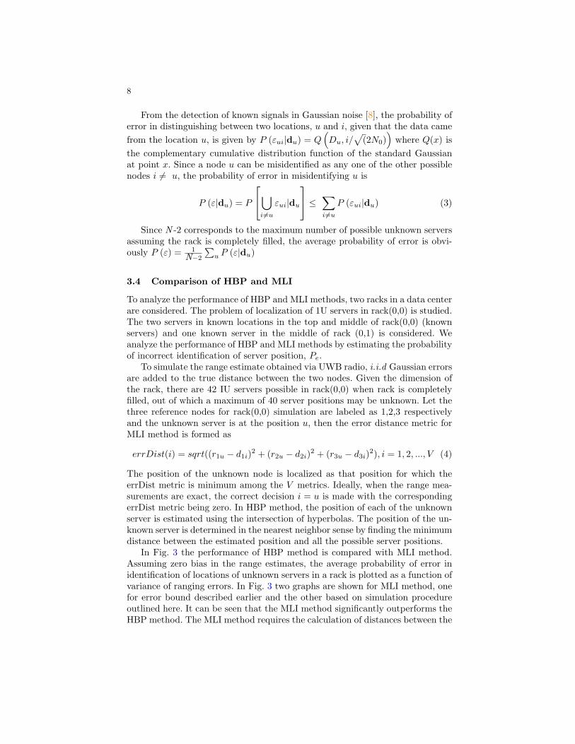
In Fig. 3 the performance of HBP method is compared with MLI method.Assuming zero bias in the range estimates, the average probability of error inidentification of locations of unknown servers in a rack is plotted as a function ofvariance of ranging errors. In Fig. 3 two graphs are shown for MLI method, onefor error bound described earlier and the other based on simulation procedureoutlined here. It can be seen that the MLI method significantly outperforms theHBP method. The MLI method requires the calculation of distances between the

9

three known nodes and all possible hypothesized positions for the unknown nodewhereas the HBP method requires the finding of the nearest neighbor node, near-est to the estimated position obtained through hyperbolic intersection. Hence,the MLI method requires a slightly more computation per sever localization.However, since computations involve mainly the calculations of Euclidean dis-tances and ascertaining the minimum of a set of numbers, these computationscan be done quickly with a reasonable inexpensive processor. Certainly, the pro-posed localization algorithm dictates an accuracy that is not attainable with theHBP method. It is observed that, as long as the variance is below 0.8 (corre-sponding to a probability of error of less than 0.1), the union bound is extremelyclose to the simulation estimate. In rest of the paper we analyze the performanceof the MLI method only.

4 MLI Simulation Results

4.1 Single Rack Simulation

In this section, we further analyze the performance of MLI method for a singlerack. We also introduce the threshold rule based on the magnitude of errordistance metric in eqn (2).

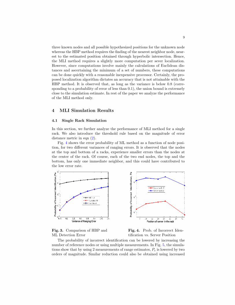
Fig. 4 shows the error probability of ML method as a function of node posi-tion, for two different variances of ranging errors. It is observed that the nodesat the top and bottom of a racks, experience smaller errors than the nodes atthe center of the rack. Of course, each of the two end nodes, the top and thebottom, has only one immediate neighbor, and this could have contributed tothe low error rate.

Fig. 3. Comparison of HBP andML Detection Error

Fig. 4. Prob. of Incorrect Iden-tification vs. Server Position

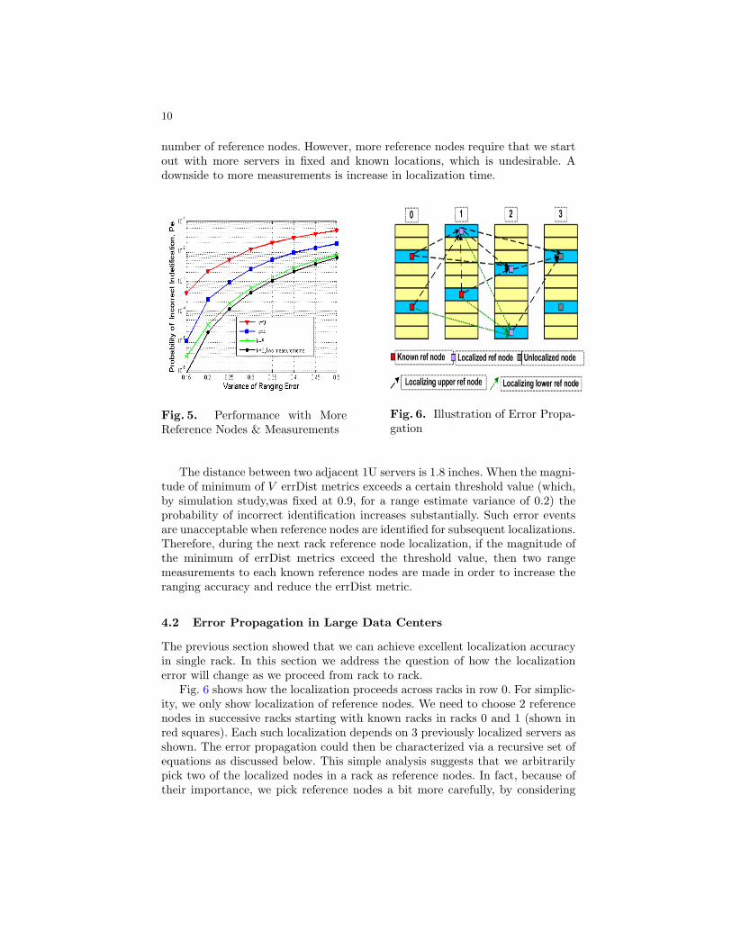
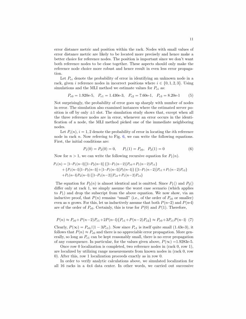
The probability of incorrect identification can be lowered by increasing thenumber of reference nodes or using multiple measurements. In Fig. 5, the simula-tions show that by using 2 measurements of range estimates, Pe is lowered by twoorders of magnitude. Similar reduction could also be obtained using increased

10

number of reference nodes. However, more reference nodes require that we startout with more servers in fixed and known locations, which is undesirable. Adownside to more measurements is increase in localization time.

Fig. 5. Performance with MoreReference Nodes & Measurements

Fig. 6. Illustration of Error Propa-gation

The distance between two adjacent 1U servers is 1.8 inches. When the magni-tude of minimum of V errDist metrics exceeds a certain threshold value (which,by simulation study,was fixed at 0.9, for a range estimate variance of 0.2) theprobability of incorrect identification increases substantially. Such error eventsare unacceptable when reference nodes are identified for subsequent localizations.Therefore, during the next rack reference node localization, if the magnitude ofthe minimum of errDist metrics exceed the threshold value, then two rangemeasurements to each known reference nodes are made in order to increase theranging accuracy and reduce the errDist metric.

4.2 Error Propagation in Large Data Centers

The previous section showed that we can achieve excellent localization accuracyin single rack. In this section we address the question of how the localizationerror will change as we proceed from rack to rack.

Fig. 6 shows how the localization proceeds across racks in row 0. For simplic-ity, we only show localization of reference nodes. We need to choose 2 referencenodes in successive racks starting with known racks in racks 0 and 1 (shown inred squares). Each such localization depends on 3 previously localized servers asshown. The error propagation could then be characterized via a recursive set ofequations as discussed below. This simple analysis suggests that we arbitrarilypick two of the localized nodes in a rack as reference nodes. In fact, because oftheir importance, we pick reference nodes a bit more carefully, by considering

11

error distance metric and position within the rack. Nodes with small values oferror distance metric are likely to be located more precisely and hence make abetter choice for reference nodes. The position is important since we don’t wantboth reference nodes to be close together. These aspects should only make thereference node choice more robust and hence result in even less error propaga-tion.

Let Pei denote the probability of error in identifying an unknown node in arack, given i reference nodes in incorrect positions where i ∈ {0, 1, 2, 3}. Usingsimulations and the MLI method we estimate values for Pei as:

Pe0 = 1.920e-5, Pe1 = 1.430e-3, Pe2 = 7.60e-1, Pe3 = 8.20e-1 (5)

Not surprisingly, the probability of error goes up sharply with number of nodesin error. The simulation also examined instances where the estimated server po-sition is off by only ±1 slot. The simulation study shows that, except when allthe three reference nodes are in error, whenever an error occurs in the identi-fication of a node, the MLI method picked one of the immediate neighboringnodes.

Let Pi(n), i = 1, 2 denote the probability of error in locating the ith referencenode in rack n. Now referring to Fig. 6, we can write the following equations.First, the initial conditions are:

P1(0) = P2(0) = 0, P1(1) = Pe0, P2(1) = 0 (6)

Now for n > 1, we can write the following recursive equation for P1(n).

P1(n) = [1−P1(n−1)][1−P2(n−1)] {[1−P1(n−2)]Pe0+P1(n−2)Pe1}+ {P1(n−1)[1−P2(n−1)]+[1−P1(n−1)]P2(n−1)} {[1−P1(n−2)]Pe1+P1(n−2)Pe2}+P1(n−1)P2(n−1) {[1−P1(n−2)]Pe2+P1(n−2)Pe3}

The equation for P2(n) is almost identical and is omitted. Since P1() and P2()differ only at rack 1, we simply assume the worst case scenario (which appliesto P1) and drop the subscript from the above equation. We now show, via aninductive proof, that P (n) remains “small” (i.e., of the order of Pe0 or smaller)even as n grows. For this, let us inductively assume that both P (n−2) and P (n−1)are of the order of Pe0. Certainly, this is true for P (0) and P (1). Therefore,

P (n) ≈ Pe0+P (n−2)Pe1+2P (n−1){Pe1+P (n−2)Pe2} ≈ Pe0+3Pe1P (n−1) (7)

Clearly, P (∞) = Pe0/(1− 3Pe1). Now since Pe1 is itself quite small (1.43e-3), itfollows that P (n) ≈ Pe0 and there is no appreciable error propagation. More gen-erally, so long as Pe1 can be kept reasonably small, there is no error propagationof any consequence. In particular, for the values given above, P (∞) =1.9283e-5.

Once row 0 localization is completed, two reference nodes in (rack 0, row 1),are localized by utilizing range measurements from known nodes in (rack 0, row0). After this, row 1 localization proceeds exactly as in row 0.

In order to verify analytic calculations above, we simulated localization forall 16 racks in a 4x4 data center. In other words, we carried out successive

12

localizations across racks using MLI along with the threshold rule for identifyingthe reference nodes. We ran the simulation 1 million times. With range estimatevariance of 0.2, the resulting localization error in 16th rack was found to be1.9286e-5, which is pretty close to the expected value.

5 Conclusions and Future Work

In this paper we proposed a wireless USB based solution for localization of allplugged-in servers in data center racks. In particular, we showed how we cansystematically locate all other nodes starting with a few known nodes and theassociated errors in doing so. We showed how the use of multiple measurementsand careful selection of reference nodes can be used to keep the error probabil-ities low in this process. For estimating the location of individual servers, weconsidered both Hyperbolic Positioning (HBP) and Maximum Likelihood iden-tification (ML) techniques. Our analysis indicates that (i) the ML method isfar superior to HBP in terms of accuracy of localization (ii) the ML method,though computationally more intense than HBP, is executable with cheap pro-cessors (iii) even with ML method, the overall accuracy critically depends ongood range estimates between a pair of UWB radios.

Future work on the topic would address the issue of reliably estimating bias indistance measurement that arises naturally due to non line of sight components.We also would like to obtain bounds on total localization time as a function ofthe data center size.

Acknowledgements: We would like to thank Anas Tom for his help withMatlab program for Union Bound.

References

1. Liu, H.; Darabi, H.; Banerjee, P.; Liu, J.; “Survey of Wireless Indoor PositioningTechniques and Systems”, IEEE Trans on Systems, Man & Cybernetics Vol. 37,Issue 6, Nov. 2007 pp.1067 - 1080

2. C. Brignone et.al ”Real Time Asset Tracking in the Data Center”, Distr. andParallel Databases, vol. 21, ISSUES 2-3, June 2007, pp.145-165.

3. Benedetto G. Maria, Giancola G.,“Understanding Ultra Wide Band Radio Funda-mentals”, Pretice Hall 2004, pp. 474-475.

4. N. Patwari, et. al., “Locating the nodes: cooperative localization in wireless sensornetworks,” IEEE Signal Process. Mag., vol. 22, Issue 4, pp. 54-69, July 2005.

5. Udar N.;, Kant K.;, Viswanathan R.;,Cheung D.;,“Ultra Wideband channel Char-acterization and Ranging in Data Center”, ICUWB 2007,Sept 2007 ,pp. 322-327.

6. Darne C., M. Macnaughtan and C. Scott, “Positioning GSM telephones”, IEEECommunications Magazine,April 1998,vol.36, Issue 4, pp. 46-54,59.

7. Yiu-Tong Chan, Yau Chin Hang, H., Pak-chung Ching, “Exact and approxi-mate Maximum Likelihood Localization Algorithms”, Vehicular Technology, IEEETransactions on Jan. 2006, vol. 55, Issue 1, pp. 10-16.

8. Seguin G.E., “A lower Bound on the Error Probability for the Signals in WhiteGaussian Noise”, textitIEEE trans on information theory, Nov. 1998, vol.4 , no. 7pp. 3168-3175.