Monograph on

Anomalies and Asset Allocation

S.P. Kothari Sloan School of Management, E52-325 Massachusetts Institute of Technology

50 Memorial Drive, Cambridge, MA 02142

(617) 253-0994 kothari@mit.edu

and

Jay Shanken

William E. Simon Graduate School of Business Administration University of Rochester, Rochester, NY 14627

(716) 275-4896 shanken@simon.rochester.edu

First draft: December 2000 Current version: June 2002

2

Acknowledgements

We thank a reviewer for helpful suggestions and Michela Verardo for excellent research assistance. We are grateful to the Research Foundation of the Institute of Chartered Financial Analysts and the Association for Investment Management and Research, the Bradley Policy Research Center at the Simon School, and the John M. Olin Foundation for financial support.

Chapter I Introduction

The issue of how an investor should combine financial investments in an overall

portfolio so as to maximize some objective is fundamental to both financial practice and to

understanding the process that determines prices in a financial market. A key principle

underlying modern portfolio theory is that there is no point in bearing portfolio risk unless

it is compensated by a higher level of expected return. This is formalized in the concept of

a mean-variance efficient portfolio, one that has as high a level of expected return as

possible for the given level of risk, and incurs the minimum risk needed to achieve that

expected return.

Although efficiency is an appealing concept, it is far from obvious just what the

composition of an efficient portfolio should be. The classic theory of risk and return called

the capital asset pricing model (CAPM) provides a starting point. It implies that the value-

weighted market portfolio of financial assets should be efficient. However, the

accumulated empirical evidence of the past two decades or so indicates that stock indices

like the S&P 500 are not (mean-variance) efficient. This literature has uncovered various

firm characteristics that are significantly related to expected returns beyond what would be

explained by their contributions to the risk of the market index. Whether this is due to

limitations of the theory or the use of a stock market index in place of the true market

portfolio, the practical implication is that one can construct portfolios that dominate the

simple market index.

Surprisingly, not much of the work exploring the empirical limitations of the

CAPM has adopted an asset allocation perspective. Rather, the focus has been on

2

measuring the magnitude of risk-adjusted expected returns.1 In this monograph, we

consider the implications for asset allocation of the three most prominent CAPM

“anomalies”: expected return effects that are negatively related to firm size (market

capitalization), and positively related to firm book-to-market ratios and past-year

momentum. For each anomaly, we estimate the amount that investors should tilt their

portfolios away from the market index, toward the anomaly-based portfolio (or spread), in

order to exploit the gains to efficiency.2 However, the same principles of modern portfolio

theory can be applied to other investment strategies that are expected to generate positive

risk-adjusted returns (e.g., an earnings-based strategy, accruals strategy, or a trading-

volume-based anomaly).

The portfolio improvement obtained by tilting an index toward an anomaly-based

strategy depends, not only on the risk-adjusted expected returns of the three strategies, but

also on residual risk, i.e., that portion of risk that is not related to variation in the market

index returns. This risk measure has received little attention in the academic literature, but

it is important for asset allocation. We also follow up on the performance of each strategy

in the second year after portfolio formation to get a rough indication of the relevance of

portfolio rebalancing. Finally, we examine asset allocation across all three anomalies and

the market index.

Our focus on the three most prominent anomalies should not be interpreted as

suggesting that we believe these anomalies will persist in the future. Each investor will

1 Two notable exceptions are the recent work of Pastor (2000), which is closely related to our analysis, and Haugen and Baker (1996). 2 For a practical guide to implementing an active portfolio investment management strategy that is grounded in modern finance, see Waring, Whitney, Pirone, and Castille (2000).

3

have his or her own beliefs about the likely performance of these and other strategies.

Traditional statistical tests of significance, while useful in many contexts, are not

particularly well suited to investment decision-making in this sort of context. In recent

years, Bayesian statistical methods have begun to achieve greater prominence in

addressing asset allocation problems.3 Part of the appeal of the Bayesian perspective is

that it provides the analyst or investor a rigorous framework in which to combine

somewhat qualitative judgments about future returns with the statistical evidence in

historical data. Such judgments or “prior beliefs” might be based on an analyst’s views

concerning the ability of financial markets to efficiently process information and the speed

with which this occurs. Related opinions about the extent to which expected returns are

compensation for risk or, instead, induced by mispricing and behavioral biases are also

relevant.

While academic literature in this area sometimes focuses on very technical

mathematical issues, the main ideas are fairly simple and very intuitive. We provide a

basic introduction to Bayesian methods, which will hopefully bring the reader close to the

state-of-the-art fairly quickly. These methods are then applied in our portfolio analysis of

expected return anomalies. Good quantitative money managers also recognize the

inevitable influence that repeated searches through the historical evidence (“data-mining”)

can have on one’s views and the need to adjust for this influence. They will typically be

inclined to try to exploit a pattern observed in past data if there is a good “story” to go with

it. We consider this issue as well.

Outline of the monograph. Chapter II reviews the finance theory on asset

allocation in the framework of the capital asset pricing model (CAPM). The chapter

3 See Kandel and Stambaugh (1996).

4

reviews portfolio theory, the CAPM, and the efficient market hypothesis. Chapter III

reviews recent evidence challenging the efficient market hypothesis. We summarize

findings suggesting economically significant profitability of trading strategies that invest in

value, momentum, and small stocks. We also discuss the implications of the evidence

indicative of market inefficiency for optimal asset allocation. Chapter IV presents the

results of our analysis of historical data and its implications for improving asset allocation

by tilting the market index toward portfolios of value, momentum, or small stocks.

Chapter V presents the intuition for and an application of a Bayesian perspective on

optimal asset allocation. Chapter VI examines the tilt portfolios’ performance over a two-

year horizon. In Chapter VII we consider the joint optimization problem in which all three

anomalies are considered simultaneously. Chapter VIII summarizes the monograph and

discusses its implications and directions for future work.

5

Chapter II

Asset allocation in a CAPM world

This chapter reviews the fundamental concepts of finance and their implications for

asset allocation. We discuss portfolio theory, the CAPM, and the efficient market

hypothesis.4

Portfolio theory

In a mean-variance setting, it is assumed that an investor’s utility increases with the

mean and decreases in the variance of overall portfolio returns.5 The mean is the expected

return on the portfolio while the variance is the measure of the portfolio’s total risk. The

efficient frontier is a graph of the set of portfolios with highest expected return for each

given level of portfolio return variance. Thus, modern portfolio theory implies that, in

order to maximize expected utility, an investor should choose a portfolio on the efficient

frontier. In 1952, Harry Markowitz developed optimization techniques for deriving the

efficient frontier of risky assets. The inputs to this derivation are estimated values of

expected return, standard deviation of return, and pairwise covariances of returns for all

available risky securities.

An investor’s portfolio selection problem is simplified with the availability of a

risk-free asset. An opportunity to invest in risky and risk-free assets implies that all

efficient portfolios consist of combinations of the risk-free asset and a unique “tangency”

4 For a detailed treatment of the concepts in this chapter, see Bodie, Kane, and Marcus (1999), chapters 6-9 and 12, or Ross, Westerfield, and Jaffe (1996), chapters 9 and 10. 5 More sophisticated approaches take into account potential hedging demands for securities (e.g., Merton, 1973, and Long, 1974) when the characteristics of the investment opportunity set change over time. Consideration of these issues is beyond the scope of this monograph.

6

portfolio of the risky assets. Investors who are relatively more risk-averse will invest a

larger fraction of their assets in the risk-free asset, whereas relatively more risk-tolerant

investors will opt for a greater fraction of their investment in the tangency portfolio. All of

these combinations of the tangency portfolio and the risk-free asset lie on a straight line

when expected return is plotted against standard deviation of return. This line, called the

capital market line, is the efficient frontier and represents the best possible combinations of

portfolio expected return and standard deviation.

The CAPM

The Capital Asset Pricing Model (CAPM) of Sharpe (1964) and Lintner (1965),

builds on Markowitz’s portfolio theory ideas and further simplifies an investor’s asset

allocation decision. The CAPM is derived with an additional critical assumption that

investors have homogenous expectations, which means that all market participants have

identical beliefs about securities’ expected returns, standard deviations, and pairwise

covariances. With homogenous expectations and the same investment horizon, all

investors would arrive at the same efficient frontier. Therefore, they would hold

combinations of the same tangency portfolio and the risk-free asset. Since total investor

demand for assets must equal the supply, in equilibrium, it follows that the tangency

portfolio is the value-weighted portfolio of all risky assets in the economy, called the

market portfolio.

The CAPM gives rise to a mathematically elegant relation between the expected

rate of return on a security and its risk relative to the market portfolio. Specifically, the

7

theory implies that expected return is an increasing linear function of its covariance risk or

beta. Beta is defined as

βi = Cov(Ri, Rm)/Var(Rm)

where Cov(Ri, Rm) is the covariance of security i’s return with the return on the market

portfolio and Var(Rm) is the variance of the return on the market portfolio. It is identical to

the (true) slope coefficient in the regression of i’s returns on those of the market and thus

indicates the relative sensitivity of security i to aggregate market movements. The CAPM

linear risk-return relation is

E(Ri) = Rf + βi (E(Rm) – Rf),

where E(Ri) is security i’s expected rate of return, Rf is the risk free rate of return, and

(E(Rm) – Rf) is the market risk premium. In addition to its importance in portfolio

analysis, beta is often used in corporate valuation and investment (i.e., capital budgeting)

decisions.

Efficient market hypothesis6

The efficient market hypothesis states that security prices rapidly and accurately

reflect all information that is available at a given point in time.7 Security markets tend

toward (informational) efficiency because a large number of market participants actively

compete among themselves to gather and process information and trade on that

information. Ideally, this process moves security prices until those prices reflect the

6 For detailed reviews of the efficient markets hypothesis and empirical literature on market efficiency, see Fama (1970, 1991) and MacKinlay (1997). 7 This notion of informational financial market efficiency should not be confused with the earlier concept of the mean-variance efficiency of a portfolio.

8

market participants’ consensus beliefs based on all of the information available to them. In

an efficient market, rewards to technical analysis and fundamental analysis are non-

existent.

In the short-run, prices may not completely adjust to new information due to

various trading costs. More generally, markets may be inefficient because of behavioral

biases in investor beliefs (excessive-optimism or pessimism, overconfidence, etc.).

Deviations from efficiency can persist if, in betting that the inefficiency will be corrected

over a given horizon, the arbitrageur is exposed to substantial risk that the “mispricing”

will get worse before it gets better.8

Portfolio theory, the CAPM, and the efficient market hypothesis jointly have

remarkably simple implications for investors’ asset allocation decisions. Investors should

hold a combination of the risky market portfolio and the risk-free asset and the investment

approach should be a passive buy-and-hold strategy (i.e., invest in index funds).9 The

picture is less clear, however, if we believe that the CAPM does not hold and if we doubt

market efficiency. We explore the attendant complexities in the remaining chapters of this

monograph.

A large body of evidence suggests that security returns exhibit significant

predictable deviations from the CAPM and that the capital markets are inefficient in

certain respects. As discussed in detail later on, these CAPM deviations or risk-adjusted

returns are captured by a statistical parameter referred to as Jensen’s alpha. Investors’

views about these capital market issues can have important implications for asset

8 See Shleifer and Vishny (2000). 9 The proportion of assets invested in the market portfolio is a function of the investor’s risk tolerance which may change endogenously with their wealth.

9

allocation by affecting their confidence that positive alphas observed in the past will persist

in the future. Therefore, we briefly review the relevant theory and evidence in the next

chapter.

10

Chapter III

Recent evidence challenging market efficiency and its implications for asset allocation

This chapter summarizes recent evidence indicating informational inefficiency in

the U.S. and international capital markets. Some of the evidence suggests capital markets

take several years to reflect information about underlying economic fundamentals in stock

prices. This evidence of apparent market inefficiency has implications for an investor’s

asset allocation decisions. Informed investors should tilt their portfolios away from the

market portfolio and in a direction that exploits the inefficiency. The optimal extent of

such tilting will depend on risk and other factors that are considered later.

Return predictability in short-window event studies

There is overwhelming evidence that security prices rapidly adjust to reflect new

information reaching the market.10 Starting with Fama, Fisher, Jensen and Roll (1969),

short-window event-study research documents the market’s quick response to new

information. This research analyzes large samples of firms experiencing a wide range of

events like stock splits, merger announcements, management changes, dividend

announcements, earnings releases, etc. There is evidence that the market reacts within

minutes of public announcements of firm-specific information like earnings and dividends

or macroeconomic information like inflation data, or interest rates. Rapid adjustment of

10 For an excellent summary of this research, see Bodie, Kane, and Marcus (1999), chapters 12 and 13.

11

prices to new information is consistent with market efficiency, but efficiency also requires

that this response is, in some sense, rational or unbiased. If both conditions hold, any

opportunity to benefit from the news is short lived and investors only earn a normal rate of

return thereafter.

Longer-horizon return predictability

In the past two decades, a large body of academic and practitioner research has

begun to challenge market efficiency.11 Mounting evidence suggests that revisions in

beliefs in response to new information do not always reflect unbiased forecasts of future

economic conditions now, and that it may take several years before prices incorporate the

full impact of the news. As the market seems to correct the initial mispricing over several

subsequent years, long-term abnormal expected returns may be possible for an informed

investor who tries to profit from this correction.

Behavioral models of investor behavior hypothesize systematic under- and over-

reaction to corporate news as a result of investors’ behavioral biases or limited capability

to process information. Barberis, Shleifer, and Vishny (1998), Daniel, Hirshleifer, and

Subramanyam (1998 and 2001), and Hong and Stein (1999) develop models to explain the

apparent predictability of stock returns at various horizons. These models draw upon

experimental evidence and theories of human judgment bias or limited information-

processing capabilities, as developed in cognitive psychology and related fields.

The representativeness bias (Kahneman and Tversky, 1982) causes people to

over-weight information patterns observed in past data, which might just be random.

11 The discussion in this chapter draws on Fama (1998).

12

Since the patterns are not really descriptive of the true properties of the underlying process,

they are not likely to persist. For example, investors might extrapolate a firm’s past history

of high sales growth and thus overreact to sales news (see Lakonishok, Shleifer, and

Vishny, 1994, and DeBondt and Thaler, 1980 and 1985).

On the other hand, investors may be slow to update their beliefs in the face of new

evidence as a result of the conservatism bias (Edwards, 1968). This can contribute to

investor under-reaction to news and lead to short-term momentum in stock prices (e.g.,

Jegadeesh, 1990, and Jegadeesh and Titman, 1993). The post-earnings announcement

drift, i.e., the tendency of stock prices to drift in the direction of earnings news for three-to-

twelve months following an earnings announcement (e.g., Ball and Brown, 1968,

Litzenberger, Joy, and Jones, 1971, and others) could also be a consequence of the

conservatism bias.

Stock price over- and under-reaction can also be an outcome of investor

overconfidence and biased self-attribution, two more human-judgment biases.

Overconfident investors place too much faith in their private information about the

company’s prospects and thus over-react to it. In the short run, overconfidence and

attribution bias (contradictory evidence is viewed as due to chance) together result in a

continuing overreaction to the initial private information that induces momentum.

Overconfidence about private information also causes investors to downplay the

importance of publicly disseminated information. Therefore, information releases like

earnings announcements generate incomplete price adjustments in this context.

Subsequent earnings outcomes eventually reveal the true implications of the earlier

evidence, however, resulting in predictable price reversals over long horizons.

13

In summary, behavioral finance theory shows how investor judgment biases can

contribute to security price over- and under-reaction to news events. The existing evidence

suggests that it can take up to several years for the market to correct the initial error in its

response to news events. These conclusions should be viewed with some skepticism,

however. The behavioral theories have, for the most part, been created to “fit the facts.”

Initially, overreaction was advanced as the main behavioral bias relevant to financial

markets. Only after the strong evidence of momentum at shorter horizons became widely

acknowledged were the more sophisticated theories developed.

As just discussed, current explanations for momentum range from underreaction to

short-term continuing overreaction. Thus, it is difficult to identify a particular behavioral

“paradigm” at this point. Moreover, recent work by Lewellen and Shanken (2002)

demonstrates that anomalous-looking patterns in returns can also arise in a model in which

fully rational investors gradually learn about certain features of the economic environment.

These patterns would be observed in the data with hindsight, but could not be exploited by

investors in real time. Clearly, sorting out all these issues is a challenging task.

Next, we review the evidence indicating return predictability. However, we caution

the reader that, in addition to the unresolved theoretical issues, there is no consensus

among academics on the interpretation of the existing empirical evidence. In particular,

Fama (1998) argues that much of the evidence on abnormal long-run return performance is

questionable because of methodological limitations and the more general effect of data

mining.

14

Evidence on return predictability

Research indicates long-horizon predictability of returns following a variety of

corporate events and past security price performance. The corporate events include stock

splits, share repurchases, extreme earnings performance announcements, bond rating

changes, dividend initiations and omissions, seasoned equity offerings, initial public

offerings, etc. Evidence of long-horizon predictability following corporate events and past

security price performance appears in the following studies (see Fama, 1998, for a detailed

discussion). Fama, Fisher, Jensen, and Roll (1969), and Ikenberry, Rankine, and Stice

(1995) examine price performance following stock splits; Ibbotson (1975) and Loughran

and Ritter (1995) study post-IPO price performance; Loughran and Ritter (1995) document

negative abnormal returns after seasoned equity offerings; Asquith (1983) and Agrawal,

Jaffe, and Mandelker (1992) estimate bidder firms’ price performance; dividend initiations

and omissions are examined in Michaely, Thaler, and Womack (1995); performance

following proxy fights is studied in Ikenberry and Lakonishok (1993); Ikenberry,

Lakonishok, and Vermaelen (1995) and Mitchell and Stafford (2000) examine returns

following open market share repurchases; and, Litzenberger, Joy, and Jones (1971), Foster,

Olsen, and Shevlin (1984) and Bernard and Thomas (1990) study post-earnings

announcement returns.

The main conclusion from these studies is that, in many cases, the magnitude of

abnormal returns is not only statistically highly significant, but economically large as well.

However, from the standpoint of asset allocation and investment strategy, predictable

returns following corporate events provide a limited opportunity to exploit the inefficiency

15

because typically only a few firms experience an event each month. Fortunately, research

also shows that a small number of firm characteristics (e.g., firm size, value and growth

attributes, i.e., the book-to-market ratio, and past price performance, i.e., momentum) are

highly successful in predicting future returns. Moreover, a large number of securities share

the firm characteristics that are correlated with substantial magnitudes of future returns.

The availability of a large pool of securities to invest in reduces the loss of diversification

entailed in trying to exploit the characteristic-based return predictability. .

The firm characteristics most highly associated with future returns are the book-to-

market ratio, firm size, and past security price performance or momentum. Banz (1981)

and, more recently, Fama and French (1993) provide evidence that small size (low market

capitalization) firms earn positive CAPM-risk-adjusted returns. That is, small firm

portfolios exhibit a positive Jensen alpha.12 Rosenberg, Lanstein, and Reid (1985) and

Fama and French (1992) show that value stocks significantly outperform growth stocks

when value is defined as the level of a firm’s book-to-market ratio. The average return of

the highest decile of stocks ranked according to book-to-market is almost one percent per

month more than for the lowest decile of stocks. The Jensen alpha of value (growth)

stocks is significantly positive (negative), both economically and statistically.13 One

possibility is that the high expected return on value stocks reflects compensation for some

sort of distress-related factor risk. An alternative interpretation is that growth stocks are

12 Handa, Kothari, and Wasley (1989) and Kothari, Shanken, and Sloan (1995) show that the size effect is mitigated when portfolios’ CAPM betas are estimated using annual returns. 13 Kothari, Shanken, and Sloan (1995) show that the book-to-market ratio effect documented in the literature is exaggerated in part because of survival biases inherent in the Compustat database and that the effect is considerably attenuated among the larger stocks and in industry portfolios.

16

overpriced glamour stocks that subsequently earn low returns (see Lakonishok, Shleifer,

and Vishny, 1994, and Haugen, 1995).

A large literature examines whether past price performance predicts future returns.

There is mixed evidence to suggest price reversal at short intervals up to a month14 and

over longer horizons of three-to-five years,15 with more compelling evidence of price

momentum at intermediate intervals of six-to-twelve months (see Jegadeesh and Titman,

1993). Only the momentum effect appears to be robust (in the post-1940 period) to the

form of risk-adjustment and other technical considerations, hence we examine the extent to

which an investor can improve the risk-return trade-off by tilting the asset allocation so as

to exploit such price momentum.

The preceding discussion identifies three characteristic-based investment strategies

that historically have produced positive abnormal returns. The next chapter presents mean-

variance optimization techniques that can be used to exploit the abnormal-return

generating ability of these anomaly-based investment strategies. However, the

optimization analysis is intended only to serve as a guiding tool for investment managers

by highlighting the potential impact of tilt strategies on portfolio risk and return. In

general, managers will also be guided by their own research, their beliefs about the

likelihood that historically successful strategies will continue to perform well in the future,

market conditions prevailing at the time of their investment decisions, and other factors

like transaction costs, international diversification, and taxes.

14 See Jegadeesh (1990), Lehmann (1990), and Ball, Kothari, and Wasley (1995). 15 See DeBondt and Thaler (1980 and 1985), Chan (1988), Ball and Kothari (1989), Chopra, Lakonishok, and Ritter (1992), Lakonishok, Shleifer, and Vishny (1994), and Ball, Kothari, and Shanken (1995).

17

Implications for asset allocation

Evidence of market inefficiency often translates into investment strategies that have

significant non-zero CAPM alphas. The intuitive implication for asset allocation is to tilt

the investment portfolio away from the passive market portfolio and toward the positive-

alpha investment strategy. The amount that we tilt the portfolio toward a particular

investment strategy would increase in the magnitude of the abnormal return from the

strategy. However, such a tilt will typically expose the investor to residual risk that

reflects return variation unrelated to the market index returns. The greater the residual risk,

the lesser the recommended tilt. The optimal asset allocation decision that accounts for the

magnitude of potential abnormal return as well as the residual risk incurred is formally

derived in a classic paper by Treynor and Black (1973) and is discussed in the next

chapter.

Our investigation of optimal asset allocation also incorporates Bayesian methods of

analysis that combine investors’ qualitative judgments about future returns with the

evidence in historical data. The qualitative judgments might be based on an investor’s

subjective assessment of the extent of market inefficiency (i.e., the magnitude of abnormal

return that might be earned in the future from an investment strategy and the speed with

which capital markets might assimilate information into future prices). In addition, there

might be a concern that the historical evidence on the magnitude of abnormal returns

exaggerates the true performance of an investment strategy because of data-mining (data-

snooping) biases inherent in the research process that might have skewed the historical

performance of an investment strategy.

18

While an analysis of the sort presented here can provide useful guidance about

asset allocation decisions, quantitative optimization techniques should not be viewed as

black boxes that produce uniquely correct answers. There are simply too many

assumptions that go into any such optimization and so there will always be an important

role for judgment in the allocation decision. Modern portfolio techniques can be an

important tool for enhancing that judgment, however. From this perspective, we believe it

is important to first explore the optimal tilt problems in detail for each of the strategies

considered here. Going through this process will give the reader a good feel for the basic

historical risk/return characteristics of these strategies in conjunction with a simple index

strategy. At the end of the monograph, we provide some additional results on optimal

portfolios based on simultaneous optimization across several strategies. This will take into

account the correlations between the various returns in addition to their individual

risk/return attributes.

19

Chapter IV

Optimal portfolio tilts

Overview

This chapter presents evidence on the historical performance of value-versus-

growth stocks, small-versus-large market capitalization stocks, and the momentum effect,

all for the past four decades. Consistent with prior research, we find that value and

positive-momentum stocks outperform growth, large-cap, and low past return stocks using

the CAPM risk-adjusted returns as the benchmark. We then examine the extent to which

tilting an investor’s portfolio in favor of value, small market capitalization, and momentum

stocks improves an investor’s risk-return trade-off.

We estimate optimal asset allocation under a variety of assumptions about the

investor’s prior beliefs concerning the efficiency of a market index and the profitability of

investing in value, small, or momentum stocks. The investor might believe that the

historical alpha of these stocks overstates their forward-looking alpha because of a

combination of factors, including data snooping, survival biases, and chance. We end this

section summarizing the results of a sensitivity analysis that includes the following.

(i) Portfolio performance over two-year horizons and an evaluation of portfolio turnover entailed in rebalancing tilt portfolios after a one-year holding period.

(ii) Results of a Bayesian predictive analysis that avoids over-fitting through

the incorporation of priors and recognition of parameter uncertainty.

(iii) Optimal asset allocation results when the market portfolio consists of both bond and equity securities.

(iv) A limited analysis of joint optimization over a market index and all three

anomaly strategies.

20

Data

We construct a comprehensive database of NYSE, AMEX, and NASDAQ equity

securities for our analysis. All firm-year observations with valid data available on the

CRSP and Compustat tapes from 1963 to 1999 are included. We measure buy-and-hold

(i.e., compounded) annual returns from July of year t to June of year t+1, starting in July

1963 (for a total of 36 years). Each year we include all firms with Compustat data

available for calculating the book-to-market ratio and CRSP data available for calculating

market capitalization and past one-year return (to assign stocks to momentum portfolios).

We require that included securities have the book-to-market ratio, size, and

momentum information prior to calculating their annual return starting on July 1.

Specifically, we measure market capitalization at the end of June of year t (e.g., size is

measured at the end of June 1963, and returns are computed for the period July 1963 –

June 1964). Book value is measured at the end of the previous fiscal year (typically,

December of the previous year, i.e., December 1962 for returns computed in July 1963 –

June 1964). The December/July gap ensures that the book value number was publicly

available at the time of portfolio formation. Following Fama-French 1993, book value is

the Compustat book value of stockholders’ equity, plus balance sheet deferred taxes and

investment tax credit (if available), plus post-retirement benefit liability (if available),

minus the book value of preferred stock. The book value of preferred stock is the

redemption, liquidation, or par value (in this order), depending on availability. The book-

to-market ratio (BM) is calculated as the book value of equity for the fiscal year ending in

calendar year t-1 divided by the market value of equity obtained at the end of June of year

t.

21

We analyze the performance of value-weighted quintile portfolios each year. We

construct these portfolios at the end of June of year t, based on size, BM, and momentum

(returns during the previous year, i.e. July t-1 to June t). Portfolios based on BM do not

include firms with negative or zero BM values. Portfolios based on momentum do not

include firms that lack return data for the 12 months preceding portfolio formation.

Some securities do not remain active for the 12-month period beginning on July 1.

Firms delist as a result of mergers, acquisitions, financial distress, and violation of

exchange listing requirements. In case of delisted securities, when available, we include

their delisting return as reported on the CRSP tapes. This prevents survival bias from

exaggerating an investment strategy’s performance.

The empirical analysis gives consideration to the practical feasibility of mutual

funds implementing the asset allocation recommendations in this monograph. Toward this

end, we therefore exclude stocks with impracticably small market capitalization and low

prices from our analysis. Investments of an economically meaningful magnitude at current

market prices can be difficult in small stocks, as they are less liquid, and low prices

typically are associated with high transaction costs. Therefore, we report results of optimal

asset allocation by restricting the universe of stocks analyzed to those with market

capitalization in excess of the smallest decile of stocks listed on NYSE and stock price

greater than $2.

Descriptive statistics

Table 1 reports descriptive statistics for the sample of equity securities that we

assemble for optimal asset allocation analysis. The total number of firm-year observations

22

from 1963 to 1998 is 100,904, with an average of about 2,800 firms per year. If we had

not excluded stocks priced lower than $2 or stocks in the lowest decile of the market

capitalization of NYSE stocks, the number of securities each year would have been

approximately 4,800. The average annual buy-and-hold return on these securities is 14%,

with a cross-sectional standard deviation of 42%. Because of some spectacular winners,

the median annual return is considerably lower at 9%.

The average return for year t-1, the year prior to investment, is reported in the last

row of Table 1 and is much higher at 22.8% compared to the average return of 14.3% for

year t. The large difference is attributable to the exclusion of low-priced and small market

capitalization stocks. Stocks experiencing negative returns decline in price and market

value by the end of year t-1. We eliminate many of those stocks as rather impractical for

investment purposes. Thus, the stocks retained for investment at the beginning of year t

have typically performed relatively well in the prior year, which naturally boosts the

average return for year t-1 of the stocks retained. Of course, all of our portfolio analysis is

forward-looking and, therefore, not subject survivor bias.

The average market capitalization of the sample securities is $723 million, but the

median stock’s market value is only $143 million.16 The mean book-to-market ratio is

1.04, which is a result of two contributing factors. First, we exclude small market

capitalization and low-priced stocks, many of which also have low book values because of

asset write-offs, restructuring charges etc., and therefore low book-to-market ratios.

Second, although book-to-market ratios in the 1990s have been at the low end of the

distribution of book-to-market ratios, book-to-market ratios in the 1970s were quite high,

16 The market capitalization numbers are not adjusted for inflation through time, so both real and nominal effects cause variation in market values across years.

23

which raises the average for our sample. Since book value data on the Compustat is not

available as frequently as return data on CRSP, there are only 75,272 firm-year

observations in the analysis using the book-to-market ratio.

Optimal tilting toward size quintile portfolios

We present evidence on large-sample historical performance of small-versus-large

market capitalization stocks, value-versus-growth stocks, and the momentum effect. To

assess the performance of each strategy, we form quintile portfolios on July 1 of each year

by ranking all available stocks on their book-to-market ratios, market capitalization, or past

one-year performance (momentum). We estimate each portfolio’s risk-adjusted

performance for the following year. We then measure the performance of a portfolio

formed by tilting the value-weight market portfolio toward the quintile portfolios, with the

weight of a quintile portfolio ranging from zero to 100% and that of the value-weight

portfolio declining from 100% to zero. That is, the value-weight portfolio is gradually

tilted all the way toward a quintile portfolio. Optimal tilt is when the Sharpe ratio of the

tilt portfolio attains the maximum.

We estimate a portfolio’s risk-adjusted performance using the CAPM regression.

The estimated intercept from a regression of portfolio excess returns on the excess value-

weight market return is the abnormal performance of the portfolio, also referred to as the

Jensen alpha. The CAPM regression is estimated using the time series of annual post-

ranking quintile portfolio returns from July 1963 to July 1998. The identity of the stocks

in each quintile portfolio changes annually as all available stocks are re-ranked each July 1

24

on the basis of their market capitalization, book-to-market ratio, or past one-year

performance. The CAPM regressions are:

Rqt – Rft = αq + βq (Rmt – Rft) + εqt (1)

where

Rqt – Rft is the buy-and-hold, value-weight excess return on quintile portfolio q for year t, defined as the quintile portfolio return minus the annual risk-free rate; Rmt – Rft is the excess return on the CRSP value-weight market return;

αq is the abnormal return (or Jensen alpha) for portfolio q over the entire estimation period; βq is the CAPM beta risk of portfolio q over the entire estimation period, and

εqt is the residual risk.

Tables 3, 4, and 5 report performance for allocations tilted toward size, book-to-

market, and momentum portfolios. Specifically, using size portfolios as an example, we

report the performance of a portfolio consisting of X% of the smallest (Q1) or largest (Q5)

market capitalization quintile portfolio and (100 – X)% of the CRSP value-weight

portfolio. X varies from 0 (i.e., no tilt toward a size quintile portfolio) to 100% (i.e., all the

investment in a size quintile portfolio).

Although probably of lesser practical relevance, we also include results for a

strategy of tilting toward the spread between quintiles 5 and 1. With the proliferation of

exchange-traded funds tied to a variety of indexes, implementing such spreads may

eventually become more realistic. The conventional size-based strategy of emphasizing

small firms would correspond to a negative position in this spread, but the risk-adjusted

performance of this small-large strategy is slightly negative for our sample. Our

25

presentation of results for the Q5-Q1 size spread will serve as an introduction to the

notation and concepts of the monograph. The more interesting findings for the Q5-Q1

value and momentum strategies will then follow.

Technically, the tilt “asset” in this context should be viewed as a position

consisting of $1 in T-bills and $1 on each side of the large-small firm spread. In other

words, the investor in this asset is implicitly assumed to receive interest on the proceeds

from the short sale of the small-firm quintile. This combined position has a net investment

of $1, unlike the spread itself, which is a zero-investment portfolio with the rate of return

undefined. Since we focus on excess returns, the return on the $1 investment in T-bills is

netted out and the performance measures are determined completely by the spread in

returns between large and small quintile stocks. The return calculations ignore the impact

of margin requirements that may be associated with either long or short positions. If the

spread portfolio generates a positive alpha, then an investor can improve performance by

tilting toward the spread. In this case, an X% “tilt toward the spread” entails a $(100 – X)

investment in the value-weight portfolio and $X in the spread asset.

We report a variety of statistics for each tilt portfolio. These include: the average

annual excess return on a tilt portfolio from 1963 to 1999; standard deviation of the excess

return; the Sharpe ratio (i.e., the ratio of the average excess return to the standard deviation

of excess return); the Jensen alpha and CAPM beta, which are estimated using regression

eq. (1). In addition to Table 3, we include figure 1 which plots the behavior of three

portfolio performance metrics (excess returns, M2, and C_M2, described below) for

portfolio allocations tilted toward the size quintile portfolios 1 and 5, and the Q5-Q1

(large-small) spread. The graphical presentation of the information is helpful in

26

visualizing the costs and benefits of tilting toward various investment strategies. The

graphs also aid in gaining an understanding of the performance metric’s sensitivity to small

deviations from the optimal portfolio. If the sensitivity is low, then the potential loss in

performance for moderate deviations from the optimum would not be great. Given the

inherent limitations of any analysis of this sort, our confidence in the relevance of the

results would be substantially reduced if too much sensitivity were observed..

The first row of the column labeled “0% = vwrt” in Table 3 shows that the average

annual excess return on the CRSP value-weight portfolio from 1963 to 1999 is 7.4%.

Values to its right are average excess returns for portfolios with increasing allocations to

the smallest size quintile portfolio, with the column labeled “100% = rt” invested entirely

in the smallest quintile portfolio. The average excess return on the smallest size quintile

portfolio is 8.6%.

This portfolio’s α is -0.5% (standard error 2.9%) and its β is 1.24 (standard error

0.15). Thus, the size effect (Banz, 1981) is not observed in this sample. The poor

performance of small stocks in the 1980s and our decision to exclude extremely low-

priced, low market capitalization stocks together result in an insignificant α for the

smallest size quintile portfolio. Without our data screen, the small firm α is 3.3%. The

row labeled “Alpha” reports Jensen alpha for the various allocations. Since the first α

value refers to the α of the value-weight portfolio, it must be zero. As the portfolio is

increasingly tilted towards the smallest quintile portfolio, the reported values approach the

α of the smallest quintile portfolio, i.e., -0.5%.

Below the portfolios’ alphas, we report their Sharpe ratios. The market portfolio’s

Sharpe ratio is 41.5%. Tilting toward small stocks dramatically lowers the Sharpe ratio,

27

with the last column showing the smallest quintile portfolio’s Sharpe ratio to be only

31.7%. The right-most column reports the ratio for the optimal portfolio with unrestricted

short-selling, i.e., the portfolio with the highest Sharpe ratio. Since tilting toward the

smallest quintile portfolio increases volatility faster than the increase in average returns,

for the 1963-1999 period, the value-weight portfolio has the optimal Sharpe ratio.

[Table 3 & Figure 1]

An equivalent measure of portfolio performance that some analysts prefer to report

is M2, which is the excess return on the portfolio after an adjustment to make its volatility

equal to that of the market index. It can be shown that M2 is a positive linear

transformation of the Sharpe ratio – hence the two performance measures provide identical

rankings of portfolios. More formally, M2 is the excess return on a hypothetical portfolio,

p*, which takes positions in the given portfolio, as well as T-bills, such that the return

volatility of p* is the same as that of the value-weight market portfolio.17 If the size-tilted

portfolio’s volatility (return standard deviation) exceeds that of the value-weight portfolio,

then p* will include a long position in T-bills so as to lower the risk.18 The return on the

resulting portfolio, p*, is referred to as M2. The value-weight portfolio’s M2 is simply its

excess return which serves as the benchmark that we hope to beat by exploiting active

positions in the anomaly-based portfolios. Since the unit of measurement for M2 is

percentage excess return, it may be a more intuitive measure than the Sharpe ratio. Table 3

shows that tilting toward the smallest size quintile portfolio results in a lower M2 than that

17 M2 is named after Franco Modigliani and Leah Modigliani. They introduced the measure in their paper appearing the Journal of Portfolio Management in 1997. 18 In the opposite situation, leverage (shorting the riskless asset) would be used to raise the volatility of p* to that of the market index. In this case, performance would be overstated insofar as the borrowing rate exceeds the T-bill rate used in the computation.

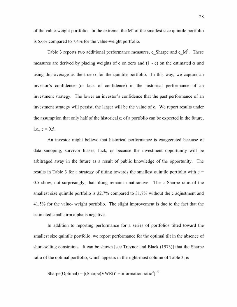
28

of the value-weight portfolio. In the extreme, the M2 of the smallest size quintile portfolio

is 5.6% compared to 7.4% for the value-weight portfolio.

Table 3 reports two additional performance measures, c_Sharpe and c_M2. These

measures are derived by placing weights of c on zero and (1 - c) on the estimated α and

using this average as the true α for the quintile portfolio. In this way, we capture an

investor’s confidence (or lack of confidence) in the historical performance of an

investment strategy. The lower an investor’s confidence that the past performance of an

investment strategy will persist, the larger will be the value of c. We report results under

the assumption that only half of the historical α of a portfolio can be expected in the future,

i.e., c = 0.5.

An investor might believe that historical performance is exaggerated because of

data snooping, survivor biases, luck, or because the investment opportunity will be

arbitraged away in the future as a result of public knowledge of the opportunity. The

results in Table 3 for a strategy of tilting towards the smallest quintile portfolio with c =

0.5 show, not surprisingly, that tilting remains unattractive. The c_Sharpe ratio of the

smallest size quintile portfolio is 32.7% compared to 31.7% without the c adjustment and

41.5% for the value- weight portfolio. The slight improvement is due to the fact that the

estimated small-firm alpha is negative.

In addition to reporting performance for a series of portfolios tilted toward the

smallest size quintile portfolio, we report performance for the optimal tilt in the absence of

short-selling constraints. It can be shown [see Treynor and Black (1973)] that the Sharpe

ratio of the optimal portfolio, which appears in the right-most column of Table 3, is

Sharpe(Optimal) = [(Sharpe(VWRt)2 +Information ratio2]1/2

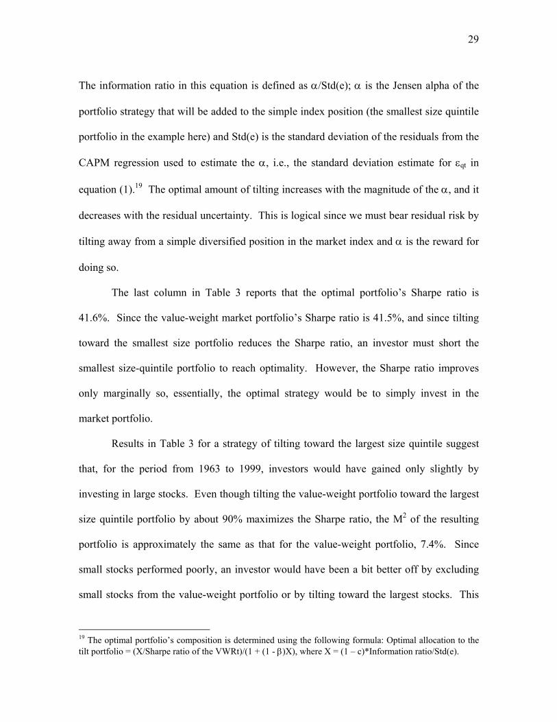
29

The information ratio in this equation is defined as α/Std(e); α is the Jensen alpha of the

portfolio strategy that will be added to the simple index position (the smallest size quintile

portfolio in the example here) and Std(e) is the standard deviation of the residuals from the

CAPM regression used to estimate the α, i.e., the standard deviation estimate for εqt in

equation (1).19 The optimal amount of tilting increases with the magnitude of the α, and it

decreases with the residual uncertainty. This is logical since we must bear residual risk by

tilting away from a simple diversified position in the market index and α is the reward for

doing so.

The last column in Table 3 reports that the optimal portfolio’s Sharpe ratio is

41.6%. Since the value-weight market portfolio’s Sharpe ratio is 41.5%, and since tilting

toward the smallest size portfolio reduces the Sharpe ratio, an investor must short the

smallest size-quintile portfolio to reach optimality. However, the Sharpe ratio improves

only marginally so, essentially, the optimal strategy would be to simply invest in the

market portfolio.

Results in Table 3 for a strategy of tilting toward the largest size quintile suggest

that, for the period from 1963 to 1999, investors would have gained only slightly by

investing in large stocks. Even though tilting the value-weight portfolio toward the largest

size quintile portfolio by about 90% maximizes the Sharpe ratio, the M2 of the resulting

portfolio is approximately the same as that for the value-weight portfolio, 7.4%. Since

small stocks performed poorly, an investor would have been a bit better off by excluding

small stocks from the value-weight portfolio or by tilting toward the largest stocks. This

19 The optimal portfolio’s composition is determined using the following formula: Optimal allocation to the tilt portfolio = (X/Sharpe ratio of the VWRt)/(1 + (1 - β)X), where X = (1 – c)*Information ratio/Std(e).

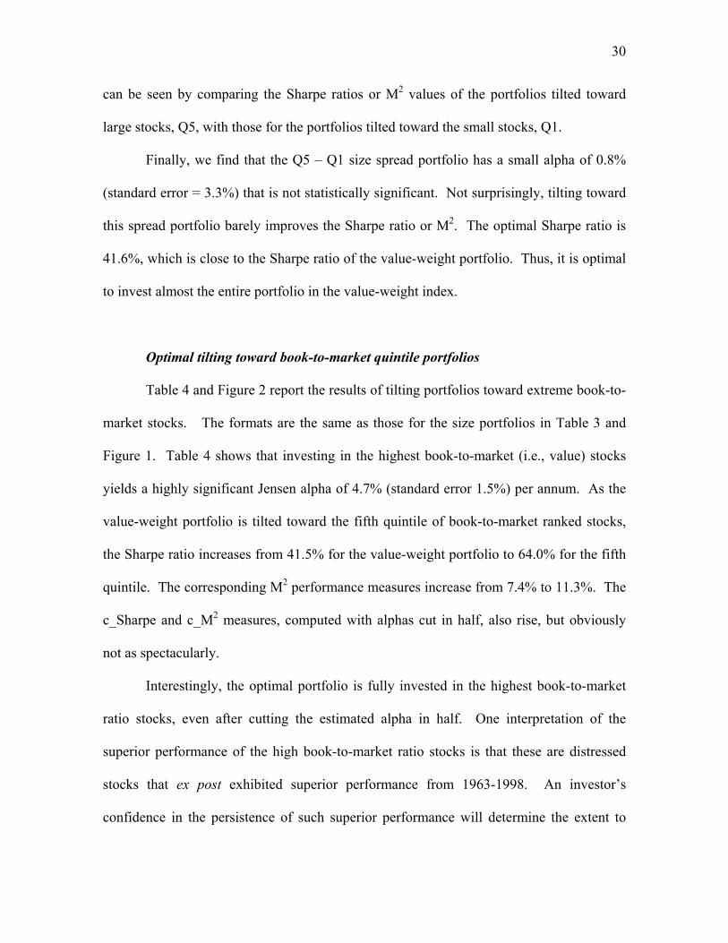
30

can be seen by comparing the Sharpe ratios or M2 values of the portfolios tilted toward

large stocks, Q5, with those for the portfolios tilted toward the small stocks, Q1.

Finally, we find that the Q5 – Q1 size spread portfolio has a small alpha of 0.8%

(standard error = 3.3%) that is not statistically significant. Not surprisingly, tilting toward

this spread portfolio barely improves the Sharpe ratio or M2. The optimal Sharpe ratio is

41.6%, which is close to the Sharpe ratio of the value-weight portfolio. Thus, it is optimal

to invest almost the entire portfolio in the value-weight index.

Optimal tilting toward book-to-market quintile portfolios

Table 4 and Figure 2 report the results of tilting portfolios toward extreme book-to-

market stocks. The formats are the same as those for the size portfolios in Table 3 and

Figure 1. Table 4 shows that investing in the highest book-to-market (i.e., value) stocks

yields a highly significant Jensen alpha of 4.7% (standard error 1.5%) per annum. As the

value-weight portfolio is tilted toward the fifth quintile of book-to-market ranked stocks,

the Sharpe ratio increases from 41.5% for the value-weight portfolio to 64.0% for the fifth

quintile. The corresponding M2 performance measures increase from 7.4% to 11.3%. The

c_Sharpe and c_M2 measures, computed with alphas cut in half, also rise, but obviously

not as spectacularly.

Interestingly, the optimal portfolio is fully invested in the highest book-to-market

ratio stocks, even after cutting the estimated alpha in half. One interpretation of the

superior performance of the high book-to-market ratio stocks is that these are distressed

stocks that ex post exhibited superior performance from 1963-1998. An investor’s

confidence in the persistence of such superior performance will determine the extent to

31

which one tilts the investment portfolio toward value stocks. Notwithstanding the potential

distressed nature of these stocks, we emphasize that we have applied the investment filter

rules that only include stocks priced greater than $2 and stocks in size deciles two through

ten. This enhances the practicality dimension of investing in these stocks.

[Table 4 and Figure 2]

Table 4 also shows that growth stocks (i.e., low book-to-market stocks) did not

perform well, though the value-weight α of -0.7% is statistically indistinguishable from

zero. As with small firms, tilting toward growth stocks lowers the Sharpe ratio and M2

measure. However, the lack of statistical significance leaves us less confident about the

potential benefits from shorting the growth stocks based on this historical performance.

The spread results for book-to-market are notable in several respects and are similar

whether we impose our small/low price filter or not. First, we now have an interior

optimum with nearly forty percent of the optimal portfolio in the spread, dropping to about

one-third when alpha is cut in half. The spread has a large alpha of 5.4%, while the spread

beta is negative: the high book-to-market quintile has a significantly lower beta than the

low book-to-market quintile. It might seem odd that average excess return declines as the

spread weight increases, despite the 5.4% alpha. This is mechanically driven by the fact

that the spread return is lower than the market return. The benefit of exploiting the small

(negative) alpha for growth, by shorting quintile 1, is dwarfed by the impact of the

relatively high residual risk for growth.

It is interesting that the information ratio for the spread is much lower than that for

the high book-to-market quintile, 33% vs. 56%, even though shorting the low book-to-

market (negative alpha) stocks increases the alpha a bit. The reason is that the spread is

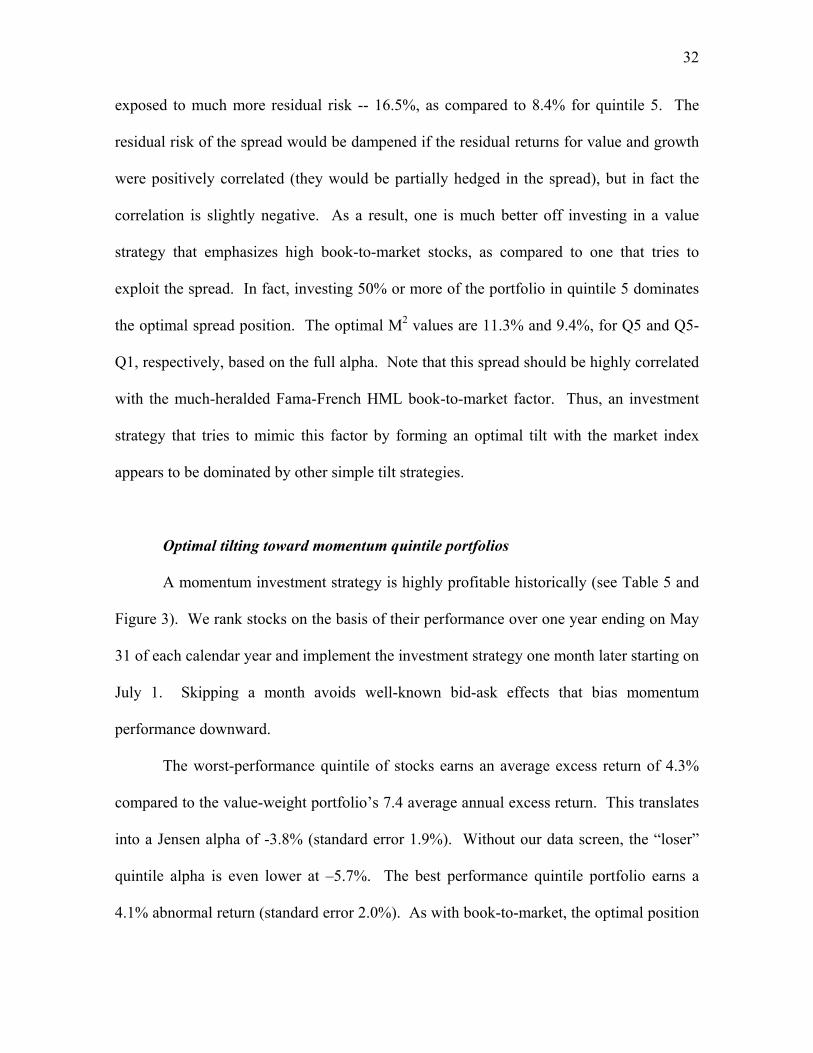
32

exposed to much more residual risk -- 16.5%, as compared to 8.4% for quintile 5. The

residual risk of the spread would be dampened if the residual returns for value and growth

were positively correlated (they would be partially hedged in the spread), but in fact the

correlation is slightly negative. As a result, one is much better off investing in a value

strategy that emphasizes high book-to-market stocks, as compared to one that tries to

exploit the spread. In fact, investing 50% or more of the portfolio in quintile 5 dominates

the optimal spread position. The optimal M2 values are 11.3% and 9.4%, for Q5 and Q5-

Q1, respectively, based on the full alpha. Note that this spread should be highly correlated

with the much-heralded Fama-French HML book-to-market factor. Thus, an investment

strategy that tries to mimic this factor by forming an optimal tilt with the market index

appears to be dominated by other simple tilt strategies.

Optimal tilting toward momentum quintile portfolios

A momentum investment strategy is highly profitable historically (see Table 5 and

Figure 3). We rank stocks on the basis of their performance over one year ending on May

31 of each calendar year and implement the investment strategy one month later starting on

July 1. Skipping a month avoids well-known bid-ask effects that bias momentum

performance downward.

The worst-performance quintile of stocks earns an average excess return of 4.3%

compared to the value-weight portfolio’s 7.4 average annual excess return. This translates

into a Jensen alpha of -3.8% (standard error 1.9%). Without our data screen, the “loser”

quintile alpha is even lower at –5.7%. The best performance quintile portfolio earns a

4.1% abnormal return (standard error 2.0%). As with book-to-market, the optimal position

33

is to be fully invested in the quintile 5 stocks. When the alpha is cut in half, the optimal

position is about 80% invested in the quintile 5 stocks, though allocations from 60% to

100% yield similar performance measures.

In contrast to what we saw for the value spread, a strategy of shorting the “losers”

and going long in the “winner” quintile results in even higher optimal Sharpe ratios and

M2s, with the optimal weight about one-half and M2 equal to 11%.20 The improvement

observed here is a reflection of the fact that the loser alpha is almost as large in magnitude

as the winner alpha. This more than offsets the increased residual risk from investing in

the spread, as reflected in the higher information ratio: 45.3% for the spread and 38.3% for

the winner quintile stocks. At very high levels of investment in the momentum spread, the

residual risk effect dominates and the performance ratios quickly deteriorate.

[Table 5 and Figure 3]

Summary

Our results on the benefits of tilting an investment portfolio toward extreme size

stocks, value and growth stocks, or momentum stocks lead to several conclusions. The

risk-return trade-off is not improved much by tilting portfolios toward extreme size stocks.

Combining the market portfolio with value (high book-to-market) stocks or past winners

(momentum) results in significant increases in the Sharpe ratio and M2. Even if an

investor believes that only half of the past positive performance of the value and

momentum strategies is sustainable in the future, such tilting strategies would be desirable.

20 The estimate of residual risk is higher than the standard deviation under “100% = rt.” This apparent contradiction is due to the degrees-of-freedom adjustments, one for total variance and two for residual variance.

34

Chapter V

The Bayesian Approach to Asset Allocation

Motivation for the Bayesian analysis.

The preceding analysis uses historical data to estimate the inputs to the asset

allocation problem and provides results for a variety of tilt strategies. However, even if we

believe that the portfolio parameters are (relatively) constant over time, it is important to

consider the potential impact of estimation error on our portfolio decisions. Unfortunately,

traditional statistical analysis is not well suited to this task. The standard errors reported

earlier can be used to derive confidence intervals for, say, alphas, but how should such

observations be translated into an investment decision?

Intuition for the Bayesian analysis.

Intuitively, if an alpha is not estimated with much precision, then it is more likely

that the apparent abnormal return (positive alpha) is due to chance and, therefore, may not

be a good indication of what will be observed in the future. In such a case, it would seem

sensible to tilt less aggressively in the direction of the given anomaly. The extent to which

we should “discount” the historical evidence because of this additional uncertainty or

estimation risk is not so clear, however.

A related issue is that we may have some prior notion as to a plausible range of

values for alpha, even before looking at the data. This prior belief could be based on

observations of returns in earlier periods or in other countries. Or, it might be based more

on economic theory and one’s general view about the efficiency of financial markets and

35

the relevance of simple theories like the CAPM.21 Recall that the CAPM implies alpha

should be zero when the index is the true market portfolio of all assets.

Whatever the source of one’s prior belief, suppose, for example, that an annualized

alpha bigger than 4% is judged implausibly large and yet an estimate of 4.7% is obtained.

In light of this prior belief, the expectation for future abnormal return is clearly less than

4.7%. Naturally, the extent to which we will want to lower or shrink the estimated value

depends on the confidence we have in our initial belief, as compared to the precision of the

statistical estimate.

Bayesian analysis provides an appealing framework in which to formalize these

ideas and incorporate them in an asset allocation decision. Academic work on portfolio

optimization has increasingly utilized Bayesian methods in recent years, the study by

Pastor (2000) being the most relevant for the issues considered here. In Bayesian analysis,

initial beliefs about return parameters are represented in terms of prior probability

distributions. For convenience, we assume normal distributions for priors as well as

returns. Using a basic law of conditional probability referred to as Bayes rule, the data are

combined with one’s initial beliefs to form an updated posterior probability distribution

that reflects the learning that has occurred from observing the data.

Implementing the Bayesian analysis for asset allocation.

For pedagogical purposes, we initially suppose that alpha is the only unknown

parameter. Let α0 be the prior expected value for alpha and σ(α0) the prior standard

deviation. Say α0 = 0, the value implied if the market index is mean-variance efficient. If

21 See Pastor (2000) for an interesting analysis of the role of a pricing model in beliefs.

36

σ(α0) = 2%, then an alpha of 4% or more is a two-standard deviation “event” with

probability less than 0.023. Of course, the actual alpha is either greater than 4% or not, but

this probability quantifies our subjective judgment that such large values are implausible.

Now, let α̂ denote the given estimate of alpha and se(α̂ ) its standard error. Say α̂

is 4.7%, as above, and se(α̂ ) = 1.5%, the values observed earlier for the high book-to-

market quintile in Table 4. In this context, Bayes rule implies that the posterior mean is a

precision-weighted average of the estimate and the prior mean:

α* = [α0 . 1/var(α0) + α̂ . 1/var(α̂ )] / [1/var(α0) + 1/var(α̂ )], (2)

where precision is technically defined as the reciprocal of variance. If the prior uncertainty

is large relative to the informativeness in the data, i.e., if var(α0) is high in relation to

var(α̂ ), Bayes rule places most of the weight on the estimate α̂ . Alternatively, if there is

not much data or if the data are quite noisy, var(α̂ ) is large and α* is closer to the prior

mean α0.

In our example, 1/var(α0) + 1/var(α̂ ) = 1/0.022 + 1/0.0152 = 2,500 + 4,444.44 =

6,944.441, so α* = (2500/6,944.44) . 0 + (4,444/6,944.44) . 0.047 = 0.03 or 3%. Since the

estimate here is a bit more precise than the prior, greater weight is placed on the estimate,

as compared to the prior mean. As a result, the posterior mean of 3% is closer to 4.7%

than to 0.

Having discussed the idea of shrinking an estimate toward a prior mean, we now

turn to the other important consideration of the impact of parameter uncertainty on risk.

We observed earlier that the optimal amount of tilting toward a quintile or spread portfolio

depends on its residual risk as well as its alpha and the Sharpe ratio of the market index.

From a Bayesian perspective, uncertainty about the true value of alpha is naturally

37

recognized as an additional source of risk that confronts an investor. Conventional risk

measures ignore this estimation risk. To convey this point, we rewrite equation (2) as a

Bayesian predictive regression:

Rq – Rf = α∗ + βq (Rm – Rf) + [εq + (αq − α∗)], (3)

where α* is the posterior mean for alpha discussed above.

Looking forward, an investor’s uncertainty about the manner in which the true

alpha deviates from its posterior expected value is a form of residual or non-market risk.

Recall that the residual term εq reflects economic influences that affect the stocks in

portfolio q, but do not have a net impact on the market index. Likewise, whether our

expected value for alpha is too high or too low will have no bearing on whether the market

subsequently goes up or down. Therefore, αq−α∗ is uncorrelated with the market return,

and with εqt as well, by a similar argument.

In order to make an optimal portfolio decision, we need to know how much

additional residual variability is induced by the “parameter uncertainty” associated with

alpha. More formally, we require the variance of the posterior probability distribution for

alpha. Fortunately, there is a simple and intuitive mathematical result that delivers this

variance: the posterior precision is just the sum of the precisions of the prior and the alpha

estimate, as given by the denominator of (2). Recalling our earlier computations, this is

6,944.44, so the posterior standard deviation, σ*(α), is 0.012 or 1.2%, as compared to the

prior standard deviation of 2%. The reduction from 2% to 1.2% is an indication of the

extent to which observing the historical data has narrowed our belief about the true value

of alpha.

38

Given the posterior standard deviation for alpha, the next step is to quantify the

overall predictive residual risk, σ*(res), perceived by the investor.22 This is the standard

deviation of the quantity in brackets in (3). Since εqt is uncorrelated with α −α∗, σ*(res)

is (0.0842 + 0.0122).5 = 8.5%. Interestingly, the uncertainty about alpha only increases the

perceived residual risk by 0.1% from the regression estimate of 8.4%. Although one might

be inclined to attribute this to the fairly tight prior distribution assumed for alpha, that is

not the cause. To see this, suppose the prior is totally uninformative, i.e., let σ(α0)

approach infinity in (2). Now, the posterior moments are identical to the sample moments:

α* = α̂ = 4.7% and σ*(α) = se(α̂ ) = 1.5%. The implied value of σ*(α) increases only

slightly, however, and is still about 8.5%. The investors’ uncertainty is just dominated by

the variability of the residual component of return in this case. Parameter uncertainty is a

second-order effect.

We make similar computations without the simplifying assumption that alpha is the

only unknown parameter in the decision problem. The relevant formulas appear in the

appendix. With uninformative priors for alpha and beta, but treating the sample residual

variance as the true value of var(εq), we have σ*(res) = 8.6%. If, instead, we let the data

dominate our belief about var(εq) and use uninformative priors for all the regression

parameters, σ*(res) increases to 8.9%.

To examine the impact of estimation risk on asset allocation, we combine the

original estimate, α̂ = 4.7%, with our most conservative estimate of residual risk, σ*(res)

= 8.9%. This risk measure now takes on the role played earlier by the regression estimate

22 In Bayesian analysis, one refers to “posterior” uncertainty when talking about parameter values and “predictive” uncertainty when the future value of a random variable like residual return, whose distribution depends on the parameters, is considered. Both concepts involve beliefs formed after observing the past data.

39

of residual standard deviation. For simplicity, we specify uninformative priors for the

mean and variance of the market index as well. By an argument similar to that for alpha

and residual risk, uncertainty about the market’s true mean return increases the (predictive)

risk perceived by the investor and lowers the perceived market Sharpe ratio. Other things

equal, this market effect tends to increase the optimal weight on the tilt portfolio.

Recall from our earlier analysis of the book-to-market anomaly, that it is optimal to

be fully invested in the high book-to-market quintile (assuming no-short-selling) when

parameter uncertainty is ignored. The corresponding M2 value was 11.3%, as compared to

the market expected return of 7.4% (market standard deviation = 17.7%). With parameter

uncertainty, being fully invested is still the optimal strategy. Now, the predictive market

risk is 18.5% and the optimal M2 is perceived to be 11.2%. The main point, however, is

that the investor is barely affected by ignoring parameter uncertainty in this case.

As a more interesting illustration, suppose we shrink the estimate of alpha with

weights c = 0.7 on zero and 0.3 on α̂ = 4.7%. The resulting value for alpha is 1.9%.

Without incorporating parameter uncertainty, the optimal weight on quintile 5 would be

74.6%, still quite high despite the more conservative assumption about alpha. The

Bayesian optimal weight is just a bit lower at 72.5%, as the increase in residual risk

apparently dominates the market risk effect. Using the “wrong” weight, 74.6%, would

reduce the perceived M2 by less than a basis point from the optimal predictive value of

7.9%. Even in this case of an unconstrained optimum, neglecting estimation risk has

virtually no effect on the investor. Only the desired degree of Bayesian shrinkage is

40

important. Similar conclusions hold for tilts involving the small firm and high momentum

quintiles.23

Summary of the Bayesian analysis.

The Bayesian analysis is a simple and intuitive approach to incorporating

information about the imprecision or uncertainty in the historical estimates of alpha or

beta. This uncertainty increases the perceived (or predictive) residual risk of the

investment portfolio. If this effect is greater than the effect of uncertainty about the market

expected return, it should incline the investor to tilt the portfolio less aggressively toward

the anomaly strategy. The preceding discussion formalizes these concepts in the context of

optimal asset allocation. We find that, under plausible assumptions, giving consideration

to parameter uncertainty changes the optimal asset allocation to some extent, but not

substantially.

23 Shrinkage implies that the prior for alpha is informative, which means that our analysis with uninformative priors overstates the impact of estimation risk in this case. Also, our conclusions are essentially unchanged if parameter uncertainty regarding the market index parameters is ignored.

41

Chapter VI

Additional Tilt-Portfolio Results

The previous analysis examined portfolio performance over the one year

immediately following the formation of the size, book-to-market, and momentum tilt

portfolios. For an investor with a longer horizon, performance measurement over one year

implicitly assumes that the optimal portfolio will be rebalanced every year. This may

entail considerable transaction costs and is only warranted if the performance of the

portfolio is likely to decay substantially over time. However, if the relevant characteristics

of stocks do not change much over the one-year holding period, then similar performance

results might be anticipated if the stock is held for an additional year. This seems plausible

for stocks ranked by size and book-to-market, but not for momentum which, by its nature,

is relatively short-lived. We now turn to some empirical evidence on this issue.

Tilt portfolio characteristics over two-year horizons

Table 6 reports transition probabilities for stocks moving from one quintile

portfolio to another in one year. The underlying data are the same as that used in optimal

portfolio construction. The second row of Table 6 shows that a stock in the smallest size

quintile has a 43.9% probability of being in the same size quintile in the following year.

The corresponding probability for the lowest book-to-market quintile is 54.4%, and it is

20.7% for the lowest quintile of momentum stocks. The transition to the “missing” cell is

quite high for stocks in all quintiles and especially so for the stocks in the first quintile.

Stocks end up in the “missing” category in year t+1 because of mergers, acquisitions,

delistings, and bankruptcies, as well as because they do not meet the investment criteria we

42

have employed (i.e., stocks priced above $2 and stocks that are not in the lowest decile of

market capitalization for NYSE stocks).

Generally, the transition probabilities for stocks ranked on momentum are roughly

the same, regardless of the initial quintile. Momentum is an indication of persistence, in

the sense that high (low) past-year quintile returns are associated with high (low) average

or expected returns for the following year. However, the realized returns in any holding

period will, like returns generally, be dominated by surprises that represent deviations from

the expected returns. Thus, conditioning on the past year’s return provides limited

information about next year’s return. Thus, a given stock is about as likely to be in one

future return (momentum) quintile as any other. In other words, the relatively uniform

transition probability distribution for momentum rankings is not surprising.

[Table 6]

The transition probabilities in Table 6 indicate that a non-trivial fraction of the

stocks in all the extreme portfolios except the large-stock portfolio end up in another

quintile portfolio after one year. Next, we present evidence on the degree to which firm

characteristics differ from their initial characteristics as a function of the investment

horizon. Table 7 reports simple averages of firm size, book-to-market ratio, and

momentum for each quintile portfolio in the formation (ranking) year t and the five

following years. The average market capitalization of the stocks in size quintile 1 is $43.3

million in the formation year t. This rises steadily from $57.3 million in year t+1 to $114.1

million in year t+5. In calculating the average market values we include all the stocks in

year t that survive in the successive future years. That is, we do not drop stocks that fail to

43

continue to meet our initial investment criteria - minimum stock price of $2 and market

capitalization in the lowest decile for NYSE stocks.

The largest size quintile stocks’ average market value increases modestly from

almost $3 billion in year t to $3.2 billion in year t+1. Value stocks, i.e., stocks in the

highest book-to-market quintile, also remain at approximately the same level in year t+1,

with the average book-to-market ratio declining from 3.0 to 2.9. Although the first-year

momentum and second-year reversal are apparent for the (simple) average returns in the

last panel of Table 7, mean-reversion after the quintile formation year is dramatic. This is

to be expected since the stocks are, by construction, ranked on their ex post realized returns

for year t, while the averages for years t+1 through t+5 provide an indication of ex ante

expected returns.

[Table 7]

The results in table 7 indicates that, if a tilt portfolio were not rebalanced at the end

of one year, its average market capitalization and book-to-market ratio would not be very

different from those of a portfolio reconstructed every year. On the other hand, the

evidence on transition probabilities in table 6 suggest that there may be some increase in

the dispersion of these characteristics over time. Ultimately, the performance of the

anomaly-based strategies over longer holding periods is an empirical question that we will

now address.

Performance of tilt portfolios over two-year horizons

The previous analysis examines portfolio performance over one year immediately

following the formation of the size, book-to-market, and momentum tilt portfolios. We

now examine performance in the second year following the tilt portfolio construction. The

44

focus is on examining whether the expected gains from tilting in the first year are sustained

in the second year without rebalancing.

To implement a strategy of investing in the second year, we sort stocks on firm

characteristics at the end of June (May, for momentum) of year t, but measure tilt portfolio

returns (using the firms that survive) starting in July of year t+1. The sample spans 35

years, and starts in July 1964. Tables 8-10 and Figures 4-6 report tilt portfolios’

performance for the second year after portfolio formation. These tables correspond to

Tables 3-5 and Figures 1-3 that report tilt portfolios’ performance for the year immediately

following their formation.

Tables 8-10 and Figures 4-6 show that tilting toward extreme size portfolios

remains unbeneficial in terms of improvement in the risk-return trade-off. The momentum

strategy exhibits signs of reversal, with an alpha of –4.1% in the second year (standard

error = 2.5%). Reversal in the second year is more consistent with momentum in the first

year being a continuation of overreaction to information that arrives during the portfolio

formation year, rather than an adjustment to an initial underreaction to information.

Value stocks (quintile 5) put forth a strong risk-adjusted performance even in the

second year after their formation (see Table 9 and Figure 5). They earn an average excess

return of 10% as compared to the value-weight market return of 7.1%. With a beta of just

0.78, the value-stock Jensen alpha is 4.5% (standard error = 1.1%), similar to the 4.7%

alpha for the first year.24 The information ratio actually increases in the second year, to

0.73 from 0.56 earlier, since residual risk declines substantially, from 8.4% to 6.2%. Since

the c_Sharpe and c_M2 are maximized at the 100% tilt, the optimal portfolio would invest

24 This is consistent with results in La Porta, Lakonishok, Shleifer, and Vishny (1997).

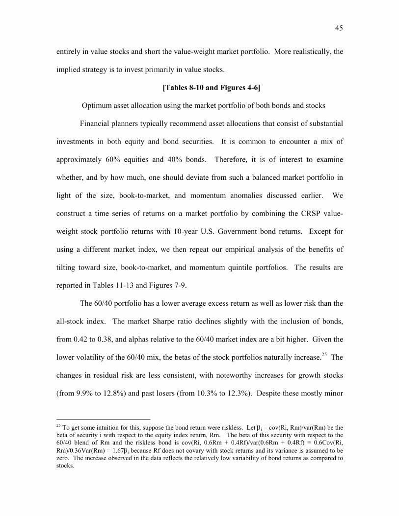
45

entirely in value stocks and short the value-weight market portfolio. More realistically, the

implied strategy is to invest primarily in value stocks.

[Tables 8-10 and Figures 4-6]

Optimum asset allocation using the market portfolio of both bonds and stocks

Financial planners typically recommend asset allocations that consist of substantial

investments in both equity and bond securities. It is common to encounter a mix of

approximately 60% equities and 40% bonds. Therefore, it is of interest to examine

whether, and by how much, one should deviate from such a balanced market portfolio in

light of the size, book-to-market, and momentum anomalies discussed earlier. We

construct a time series of returns on a market portfolio by combining the CRSP value-

weight stock portfolio returns with 10-year U.S. Government bond returns. Except for

using a different market index, we then repeat our empirical analysis of the benefits of

tilting toward size, book-to-market, and momentum quintile portfolios. The results are

reported in Tables 11-13 and Figures 7-9.

The 60/40 portfolio has a lower average excess return as well as lower risk than the

all-stock index. The market Sharpe ratio declines slightly with the inclusion of bonds,

from 0.42 to 0.38, and alphas relative to the 60/40 market index are a bit higher. Given the

lower volatility of the 60/40 mix, the betas of the stock portfolios naturally increase.25 The

changes in residual risk are less consistent, with noteworthy increases for growth stocks

(from 9.9% to 12.8%) and past losers (from 10.3% to 12.3%). Despite these mostly minor

25 To get some intuition for this, suppose the bond return were riskless. Let βi = cov(Ri, Rm)/var(Rm) be the beta of security i with respect to the equity index return, Rm. The beta of this security with respect to the 60/40 blend of Rm and the riskless bond is cov(Ri, 0.6Rm + 0.4Rf)/var(0.6Rm + 0.4Rf) = 0.6Cov(Ri, Rm)/0.36Var(Rm) = 1.67βi because Rf does not covary with stock returns and its variance is assumed to be zero. The increase observed in the data reflects the relatively low variability of bond returns as compared to stocks.

46

changes, the implications for tilting and optimal asset allocation are quite similar to those

discussed earlier with the all-stock market portfolio: heavy tilts toward value and high

momentum stocks, with less aggressive tilts toward the value and momentum spreads due

to the moderating effect of residual risk.

[Tables 11-13 and Figures 7-9]

47

Chapter VII

Optimal asset allocation with all-three-anomaly strategies

In this chapter, we consider the optimal asset allocation for two sets of risky assets:

i) the stock market index, large firms, value firms, and high momentum firms, and ii) the

stock market index, the size spread (large-small), the value spread (high-low book-to

market), and the momentum spread (winners-losers). The individual risk and return

characteristics of these assets were examined in Chapter 4. The correlations between

portfolio residual returns are also relevant to the joint optimization problem. The

estimated residual correlation between large firms and value firms is -0.30. The residual

correlation between the book-to-market and momentum (size) spreads is -0.27 (-0.20).

The other correlations are also negative but closer to zero.

Following Treynor and Black (1973), we structure the asset allocation decision in

terms of an optimal active portfolio of the anomaly-based investments and an optimal

combination of the market index and the active portfolio.26 Based on the historical

estimates, the optimal strategy for the first set of assets entails an “unreasonably” large

(-563%) short position in the market index. In fact, even if we let c = 0.9 and reduce all

the alphas by 90%, the optimal strategy still shorts the market. When short selling is ruled

out, the active portfolio (c = 0) consists of 77% in value firms and 23% in winner firms and

the optimal portfolio has no (direct) investment in the stock market index. This is depicted

graphically in Figure 10. The optimal M2 is 11.5%, much higher than the 7.4% excess

26 In the unrestricted short-selling case, we use the formulas in Gibbons, Ross, and Shanken (1989), which generalize those in Treynor and Black (1973) to accommodate nonzero residual correlation.

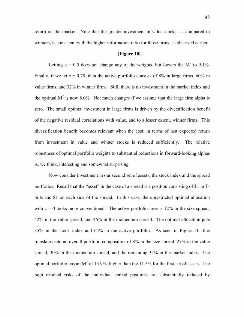
48

return on the market. Note that the greater investment in value stocks, as compared to

winners, is consistent with the higher information ratio for those firms, as observed earlier.

[Figure 10]

Letting c = 0.5 does not change any of the weights, but lowers the M2 to 9.1%.

Finally, if we let c = 0.75, then the active portfolio consists of 8% in large firms, 60% in

value firms, and 32% in winner firms. Still, there is no investment in the market index and

the optimal M2 is now 8.0%. Not much changes if we assume that the large firm alpha is

zero. The small optimal investment in large firms is driven by the diversification benefit

of the negative residual correlations with value, and to a lesser extent, winner firms. This

diversification benefit becomes relevant when the cost, in terms of lost expected return

from investment in value and winner stocks is reduced sufficiently. The relative

robustness of optimal portfolio weights to substantial reductions in forward-looking alphas

is, we think, interesting and somewhat surprising.

Now consider investment in our second set of assets, the stock index and the spread

portfolios. Recall that the “asset” in the case of a spread is a position consisting of $1 in T-

bills and $1 on each side of the spread. In this case, the unrestricted optimal allocation

with c = 0 looks more conventional. The active portfolio invests 12% in the size spread,

42% in the value spread, and 46% in the momentum spread. The optimal allocation puts

35% in the stock index and 65% in the active portfolio. As seen in Figure 10, this

translates into an overall portfolio composition of 8% in the size spread, 27% in the value

spread, 30% in the momentum spread, and the remaining 35% in the market index. The

optimal portfolio has an M2 of 13.9%, higher than the 11.5% for the first set of assets. The

high residual risks of the individual spread positions are substantially reduced by

49

diversifying across spreads, making it possible to exploit the high alphas more efficiently

than with the single-spread tilts examined in Chapter IV.

In general, when short selling is not restricted, it can be shown algebraically that

increasing c leaves the active portfolio unchanged. Naturally, the weight on the active

portfolio is lowered, however. With c = 0.5 (0.75), that weight is 54% (40%), down from

65%, and the corresponding M2 drops to 9.4% (7.9%) from the 13.9% value when c = 0.

While reduced, we still see a strong role for the anomaly-based strategies even after

substantial reductions in the historical alphas.

50

Chapter VIII

Summary, conclusions, and directions for future research

Our main findings are as follows. First, there is essentially no size effect in our

data over the period 1963-98. This is due, in part, to our exclusion of very small, low-

priced stocks in an attempt to approximate realistic investment strategies. As in earlier

work, the book-to-market and momentum effects are large. When we rank stocks from

low to high and form quintiles, the spreads in alpha between quintiles 5 and 1 are 5.4% and

8.0%, respectively. Considering the anomalies separately and examining feasible

strategies involving either high book-to-market (value) or strong momentum stocks, the

optimal allocation is to be fully invested in quintile 5. Moreover, this is true for value even

if we inject a healthy dose of conservatism and reduce the alphas by half! The optimal tilt

toward strong momentum stocks is about 80% with the reduced alpha.

Less extreme optimal tilts are obtained when the Q5 – Q1 spreads (i.e., long in

quintile 5 and short in quintile 1) are considered, although these strategies would seem less

relevant from a practical investment perspective. Interestingly, the residual risk of the

value spread portfolio is so high that an investor would be better off with an aggressive

position in high book-to-market stocks as compared to an optimal spread position. Thus,

despite the higher alpha of the spread portfolio, i.e., our version of the Fama-French HML

factor portfolio, its risk-return characteristics are not as attractive as those of the high

book-to-market portfolio when considered solely in combination with the value-weight

market portfolio.

The tenor of our results is unchanged when a 60/40 market index of stocks and

bonds is used. We also track the performance of each strategy in the second year after

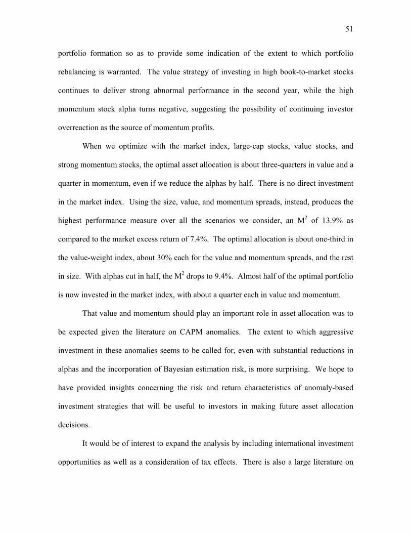
51

portfolio formation so as to provide some indication of the extent to which portfolio

rebalancing is warranted. The value strategy of investing in high book-to-market stocks

continues to deliver strong abnormal performance in the second year, while the high

momentum stock alpha turns negative, suggesting the possibility of continuing investor

overreaction as the source of momentum profits.

When we optimize with the market index, large-cap stocks, value stocks, and

strong momentum stocks, the optimal asset allocation is about three-quarters in value and a

quarter in momentum, even if we reduce the alphas by half. There is no direct investment

in the market index. Using the size, value, and momentum spreads, instead, produces the

highest performance measure over all the scenarios we consider, an M2 of 13.9% as

compared to the market excess return of 7.4%. The optimal allocation is about one-third in

the value-weight index, about 30% each for the value and momentum spreads, and the rest

in size. With alphas cut in half, the M2 drops to 9.4%. Almost half of the optimal portfolio

is now invested in the market index, with about a quarter each in value and momentum.

That value and momentum should play an important role in asset allocation was to

be expected given the literature on CAPM anomalies. The extent to which aggressive

investment in these anomalies seems to be called for, even with substantial reductions in

alphas and the incorporation of Bayesian estimation risk, is more surprising. We hope to

have provided insights concerning the risk and return characteristics of anomaly-based

investment strategies that will be useful to investors in making future asset allocation

decisions.

It would be of interest to expand the analysis by including international investment

opportunities as well as a consideration of tax effects. There is also a large literature on

52

stock return predictability that documents changes in risk and expected return over time.

Incorporating this sort of information might lead to improved asset allocation decisions.

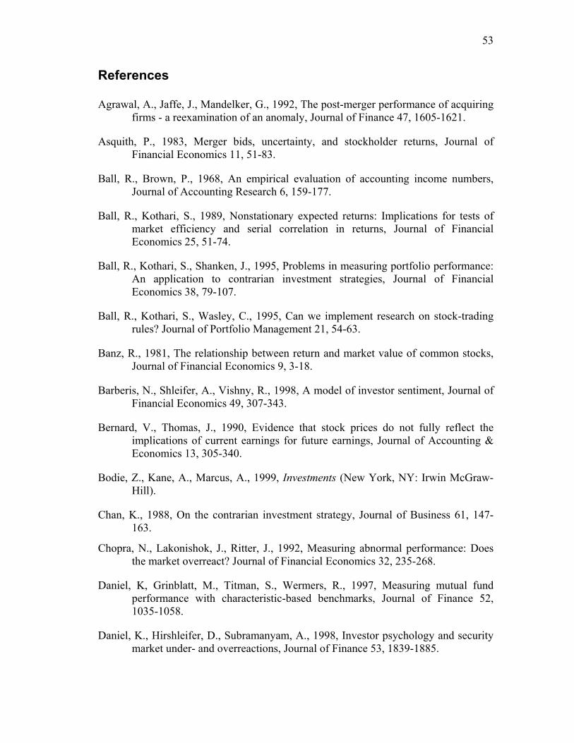
53

References

Agrawal, A., Jaffe, J., Mandelker, G., 1992, The post-merger performance of acquiring firms - a reexamination of an anomaly, Journal of Finance 47, 1605-1621.

Asquith, P., 1983, Merger bids, uncertainty, and stockholder returns, Journal of Financial Economics 11, 51-83.

Ball, R., Brown, P., 1968, An empirical evaluation of accounting income numbers, Journal of Accounting Research 6, 159-177.

Ball, R., Kothari, S., 1989, Nonstationary expected returns: Implications for tests of market efficiency and serial correlation in returns, Journal of Financial Economics 25, 51-74.

Ball, R., Kothari, S., Shanken, J., 1995, Problems in measuring portfolio performance: An application to contrarian investment strategies, Journal of Financial Economics 38, 79-107.

Ball, R., Kothari, S., Wasley, C., 1995, Can we implement research on stock-trading rules? Journal of Portfolio Management 21, 54-63.

Banz, R., 1981, The relationship between return and market value of common stocks, Journal of Financial Economics 9, 3-18.

Barberis, N., Shleifer, A., Vishny, R., 1998, A model of investor sentiment, Journal of Financial Economics 49, 307-343.

Bernard, V., Thomas, J., 1990, Evidence that stock prices do not fully reflect the implications of current earnings for future earnings, Journal of Accounting & Economics 13, 305-340.

Bodie, Z., Kane, A., Marcus, A., 1999, Investments (New York, NY: Irwin McGraw-Hill).

Chan, K., 1988, On the contrarian investment strategy, Journal of Business 61, 147-163.

Chopra, N., Lakonishok, J., Ritter, J., 1992, Measuring abnormal performance: Does the market overreact? Journal of Financial Economics 32, 235-268.

Daniel, K, Grinblatt, M., Titman, S., Wermers, R., 1997, Measuring mutual fund performance with characteristic-based benchmarks, Journal of Finance 52, 1035-1058.

Daniel, K., Hirshleifer, D., Subramanyam, A., 1998, Investor psychology and security market under- and overreactions, Journal of Finance 53, 1839-1885.

54

Daniel, K., Hirshleifer, D., Subramanyam, A., 2001, Overconfidence, arbitrage, and equilibrium asset pricing, Journal of Finance 56, 921-965.

DeBondt, W., Thaler, R., 1985, Does the stock market overreact? Journal of Finance 40, 793-805.

DeBondt, W., Thaler, R., 1987, Further evidence of investor overreaction and stock market seasonality, Journal of Finance 42, 557-581.

Edwards, W., 1968, Conservatism in human information processing, In: Kleinmutz, B. (Ed.), Formal Representation of Human Judgement (New York, NY: Wiley).

Fama, E., 1965, The behavior of stock market prices, Journal of Business 38, 34-105.

Fama, E., 1970, Efficient capital markets: A review of theory and empirical work, Journal of Finance 25, 383-417.

Fama, E., 1990, Stock returns, expected returns, and real activity, Journal of Finance 45,1089-1108.

Fama, E., 1991, Efficient capital markets: II, Journal of Finance 46, 1575-1617.

Fama, E., 1998, Market efficiency, long-term returns, and behavioral finance, Journal of Financial Economics 49, 283-306.

Fama, E., Fisher, L., Jensen, M., Roll, R., 1969, The adjustment of stock prices to new information, International Economic Review 10, 1-21.

Fama, E., French, K., 1988, Permanent and temporary components of stock prices, Journal of Political Economy 96, 246-273.

Fama, E., French, K., 1989, Business conditions and expected returns on stocks and bonds, Journal of Financial Economics 25, 23-49.

Fama, E., French, K., 1993, Common risk factors in the returns on stocks and bonds, Journal of Financial Economics 33, 3-56.

Fama, E., French, K., 1996, Multifactor explanations of asset pricing anomalies, Journal of Finance 51, 55-84.

Fama, E., French, K., 1992, The cross-section of expected returns, Journal of Finance 47, 427-465.

Fama, E., MacBeth, J., 1973, Risk, return, and equilibrium: Empirical tests, Journal of Political Economy 81, 607-636.

Foster, G., Olsen, C., Shevlin, T., 1984, Earnings releases, anomalies and the behavior of security returns, The Accounting Review 59, 574-603.

55

Handa, P., Kothari, S., Wasley, C., 1989, The relation between the return interval and betas: Implications for the size effect, Journal of Financial Economics 23, 79-100.

Haugen, R., 1995, The New Finance: The Case Against Efficient Markets (Englewood Cliffs, NJ: Prentice Hall).

Haugen, R., Baker, N., 1996, Commonality in the Determinants of Expected Returns, Journal of Financial Economics.

Hong, H., Stein, J., 1999, A unified theory of underreaction, momentum trading, and overreaction in asset markets, Journal of Finance 54, 2143-2184.

Ibbotson, R., 1975, Price performance of common stock new issues, Journal of Financial Economics 2, 235-272.

Ikenberry, D., Lakonishok, J., 1993, Corporate governance through the proxy contest: evidence and implications, Journal of Business 66, 405-435.

Ikenberry, D., Lakonishok, J., Vermaelen, T., 1995, Market underreaction to open market share repurchases, Journal of Financial Economics 39, 181-208.

Ikenberry, D., Rankine, G., Stice, E., 1995, What do stock splits really signal? Journal of Financial and Quantitative Analysis 31, 357-375.

Jegadeesh, N., 1990, Evidence of predictable behavior of security returns, Journal of Finance 45, 881-898.

Jegadeesh, N., Titman, S., 1993, Returns to buying winners and selling losers: Implications for stock market efficiency, Journal of Finance 48, 65-91.

Kahneman, D., Tversky, A., 1982, Intuitive predictions: Biases and corrective procedures, Reprinted in Kahneman, Slovic, and Tversky, Judgement under Uncertainty: Heuristics and Biases, (Cambridge, England: Cambridge University Press).

Kandel, S., Stambaugh, R., 1996, On the predictability of stock returns: An asset allocation perspective, Journal of Finance 51, 385-424.

Kothari, S., Shanken, J., Sloan, R., 1995, Another look at the cross-section of expected returns, Journal of Finance 50, 185-224.

Lakonishok, J., Shleifer, A., Vishny, R., 1994, Contrarian investment, extrapolation, and risk, Journal of Finance 49, 1541-1578.

La Porta, R., Lakonishok, J., Shleifer, A., Vishny, R., 1997, Good news for value stocks: further evidence on market efficiency, Journal of Finance 52, 859-874.

56

Lehmann, B., 1990, Fads, martingales, and market efficiency, Quarterly Journal of Economics 105, 1-28.

Lewellen, J., Shanken, J., 2002, Learnings, asset-pricing tests, and market efficiency, Journal of Finance 57, 1113-1145.

Lintner, J., 1965, The valuation of risky assets and the selection of risky investments in stock portfolios and capital budgets, Review of Economics and Statistics 47, 13-37.

Litzenberger, R., Joy, M., Jones, C., 1971, Ordinal predictions and the selection of common stocks, Journal of Financial and Quantitative Analysis 6, 1059-1068.

Long, J., 1974, Stock prices, inflation, and the term structure of interest rates, Journal of Financial Economics 1, 131-170.

Loughran, T., Ritter, J., 1995,The new issues puzzle, Journal of Finance 50, 23-51.

MacKinlay, A., 1997, Event studies in economics and finance, Journal of Economic Literature 35, 13-39.

Markowitz, H., 1952, Portfolio selection, Journal of Finance 7, 77-91.

Merton, R., 1973, Intertemporal capital asset pricing model, Econometrica 41, 867-887.

Michaely, R., Thaler, R., Womack, K., 1995, Price reactions to dividend initiations and omissions: overreaction or drift, Journal of Finance 50, 997-997.

Mitchell, M., Stafford, E., 2000, Managerial decisions and long-term stock price performance, Journal of Business 73, 287-329.

Modigliani, F., Modigliani, L., 1997, Risk-adjusted performance, Journal of Portfolio Management, 45-54.

Mossin, J., 1966, Equilibrium in a capital asset market, Econometrica 34, 768-783.

Pastor, L., 2000, Portfolio slection and asset pricing models, Journal of Finance 55, 179-223.

Rosenberg, B., Reid, K., Lanstein, R., 1985, Persuasive evidence of market inefficiency, Journal of Portfolio Management 11, 9-17.

Ross, S., Westerfield, R., Jaffee, J., 1996, Corporate Finance, 4th edition, Mc-Graw-Hill, New York, NY.

Sharpe, W., 1964, Capital asset prices: A theory of market equilibrium under conditions of risk, Journal of Finance 19, 425-442.

57

Shleifer, A., Vishny, R., 1997, The limits of arbitrage, Journal of Finance 52, 35-55.

Treynor, J., Black, F., 1973, How to use security analysis to improve portfolio selection? Journal of Business 46, 66-86.

Waring, B., Whitney, D., Pirone, J., Catille, C., 2000, Optimizing manager structure and budgeting manager risk, The Journal of Portfolio Management, 90-104.

58

Appendix

First, we evaluate the predictive residual variance assuming that the priors for alpha

and beta are uninformative, the residual standard deviation is known, and returns are

jointly normally distributed. In this case, it is well known that the posterior distribution of

the regression parameters mirrors the usual sampling distribution for the regression

estimates; i.e., (α, β) is jointly normally distributed with mean (α̂ , β̂ ) and variance matrix

σ2(ε).(X'X)-1, where X is the Tx2 matrix of independent variables including a constant

vector (Zellner, 1971).

Consider the regression equation of quintile excess return on the market index

excess return. We use the simpler notation, yt = α + βxt + εt . For out-of-sample return

observations, x and y, the corresponding predictive regression is

y = α̂ + β̂ x + [ε + (α−α̂ ) + (β− β̂ )x], (Α1)

where α̂ and β̂ are regression estimates based on data from t=1 to T. From the Bayesian

perspective, these estimates are the predictive regression coefficients (α* and β* in our

earlier notation) and the expression in brackets is the predictive regression residual. As

before, the residual consists of the regression disturbance plus additional terms that reflect

uncertainty about the parameters α and β.

The predictive residual can be viewed as the difference between y and the

regression-based prediction of y conditional on a known value of x. This is referred to as

the prediction error in standard regression analysis. Its conditional variance is well known

and given by the expression:

var(ε){1 + [1 + (x - x )2/sx2]/T}, (A2)

where x is the sample mean and sx2

the variance of the market returns (maximum

likelihood estimates).

Whereas x is known in the classical prediction problem, the future market return is

yet to be realized when making the asset allocation decision. Therefore, the relevant

predictive residual variance for the quintile return y is the average value of the variance in

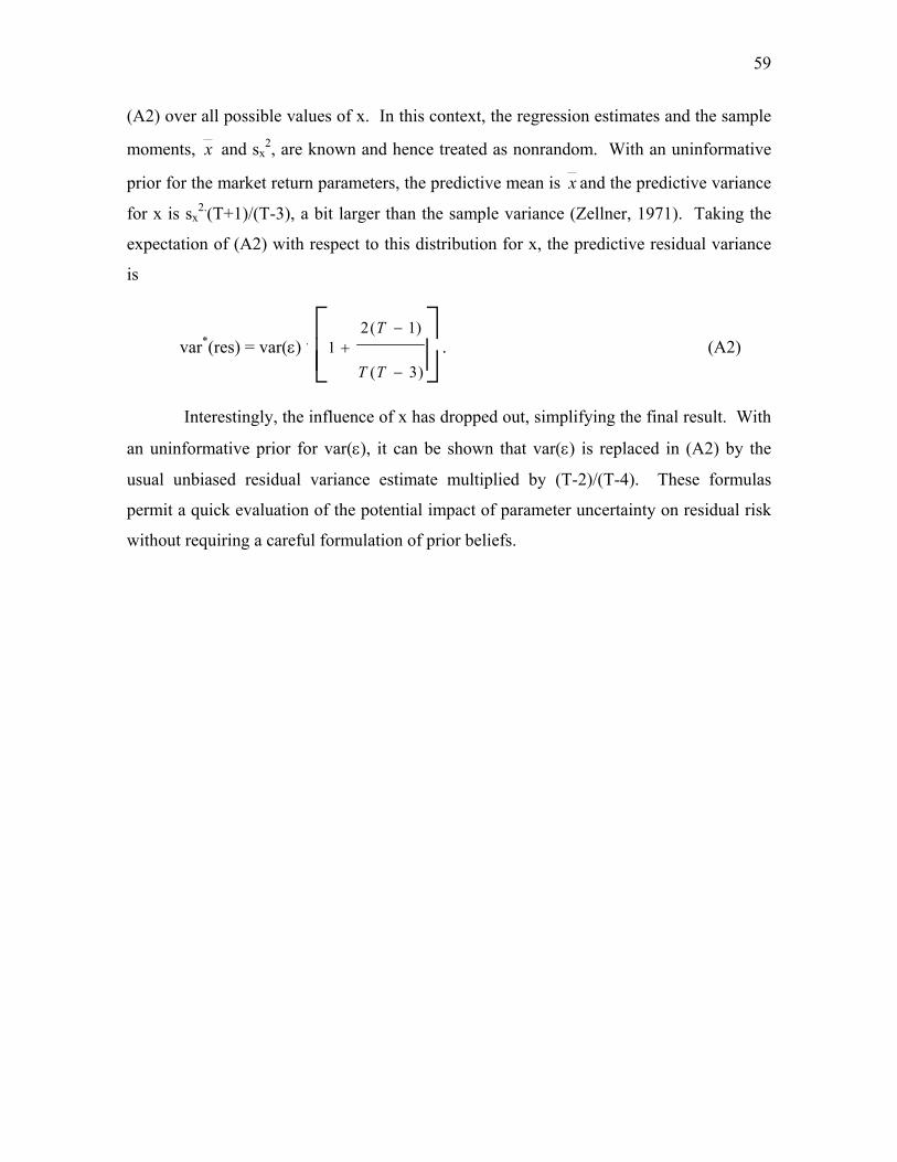
59

(A2) over all possible values of x. In this context, the regression estimates and the sample

moments, x and sx2, are known and hence treated as nonrandom. With an uninformative

prior for the market return parameters, the predictive mean is x and the predictive variance

for x is sx2.(T+1)/(T-3), a bit larger than the sample variance (Zellner, 1971). Taking the

expectation of (A2) with respect to this distribution for x, the predictive residual variance

is

var*(res) = var(ε) .

−

−+

)3(

)1(21

TT

T. (A2)

Interestingly, the influence of x has dropped out, simplifying the final result. With

an uninformative prior for var(ε), it can be shown that var(ε) is replaced in (A2) by the

usual unbiased residual variance estimate multiplied by (T-2)/(T-4). These formulas

permit a quick evaluation of the potential impact of parameter uncertainty on residual risk

without requiring a careful formulation of prior beliefs.

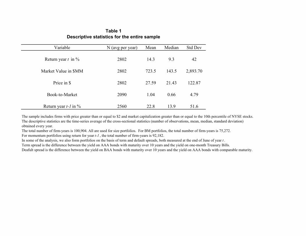
Variable N (avg per year) Mean Median Std Dev

Return year t in % 2802 14.3 9.3 42

Market Value in $MM 2802 723.5 143.5 2,893.70

Price in $ 2802 27.59 21.43 122.87

Book-to-Market 2090 1.04 0.66 4.79

Return year t-1 in % 2560 22.8 13.9 51.6

obtained every year.

For momentum portfolios using return for year t-1 , the total number of firm-years is 92,182.

Table 1Descriptive statistics for the entire sample

The descriptive statistics are the time-series average of the cross-sectional statistics (number of observations, mean, median, standard deviation)

Deafult spread is the difference between the yield on BAA bonds with maturity over 10 years and the yield on AAA bonds with comparable maturity.

The sample includes firms with price greater than or equal to $2 and market capitalization greater than or equal to the 10th percentile of NYSE stocks.

The total number of firm-years is 100,904. All are used for size portfolios. For BM portfolios, the total number of firm-years is 75,272.

In some of the analysis, we also form portfolios on the basis of term and default spreads, both measured at the end of June of year t . Term spread is the difference between the yield on AAA bonds with maturity over 10 years and the yield on one-month Treasury Bills.

rt Anomaly-based active portfolio: size, book-to-market, or momentum extreme quintiles/spreads.

exrt Time series average of annual excess returns on a tilt portfolio (over 36 years, 1964-1999). Excess return is the raw portfolio return minus the one-year riskless rate.

10%, 20% .. Percentage of rt in each tilt-portfolio return. 0% corresponds to the value-weighted market return, 100% to rt.

std(exrt) Standard deviation of excess return.

Alpha Intercept from a CAPM regression of excess active portfolio return on the excess market return. The alpha ofeach tilt portfolio is a fraction of the alpha of the active portfolio, e.g., alpha for 10% tilt is 10%* (alpha of rt).

Sharpe Sharpe ratio = exrt/std(exrt).

c Measure of an investor's lack of confidence in historical performance. c = 0.5 is used, which means that prospective asset allocations are based on 50% of the historical alpha estimates.

c_Sharpe Sharpe ratio based on reduced alpha = (exrt - c*alpha)/std(exrt) .

M2 M-square measure of performance = Sharpe * std(market excess return) = excess return on a combination of the active portfolio and the riskless asset that has the same standard deviation as the market portfolio.

c_M2 M-square measure based on reduced alpha = c_Sharpe * std(market excess return).

Table 2Legend for all tables in the Monograph

Beta Slope coefficient from a CAPM regression of excess active portfolio return on the excess market return.

std(eA) Standard deviation of residuals from the CAPM regression for active portfolio A.

Shp mkt Sharpe ratio of the value-weight market portfolio.

Info ratio Information ratio = alpha/std(eA).

Shp opt Sharpe ratio of the optimal portfolio with unrestricted short-selling and confidence level c = sqrt(Shp_mkt^2 + [(1-c) * (alpha/std(eA))]^2).

Standard errors Standard errors are given below each estimate.For alpha and beta, the standard errors come from the regression.For Sharpe ratios and information ratios, approximate standard errors are given.

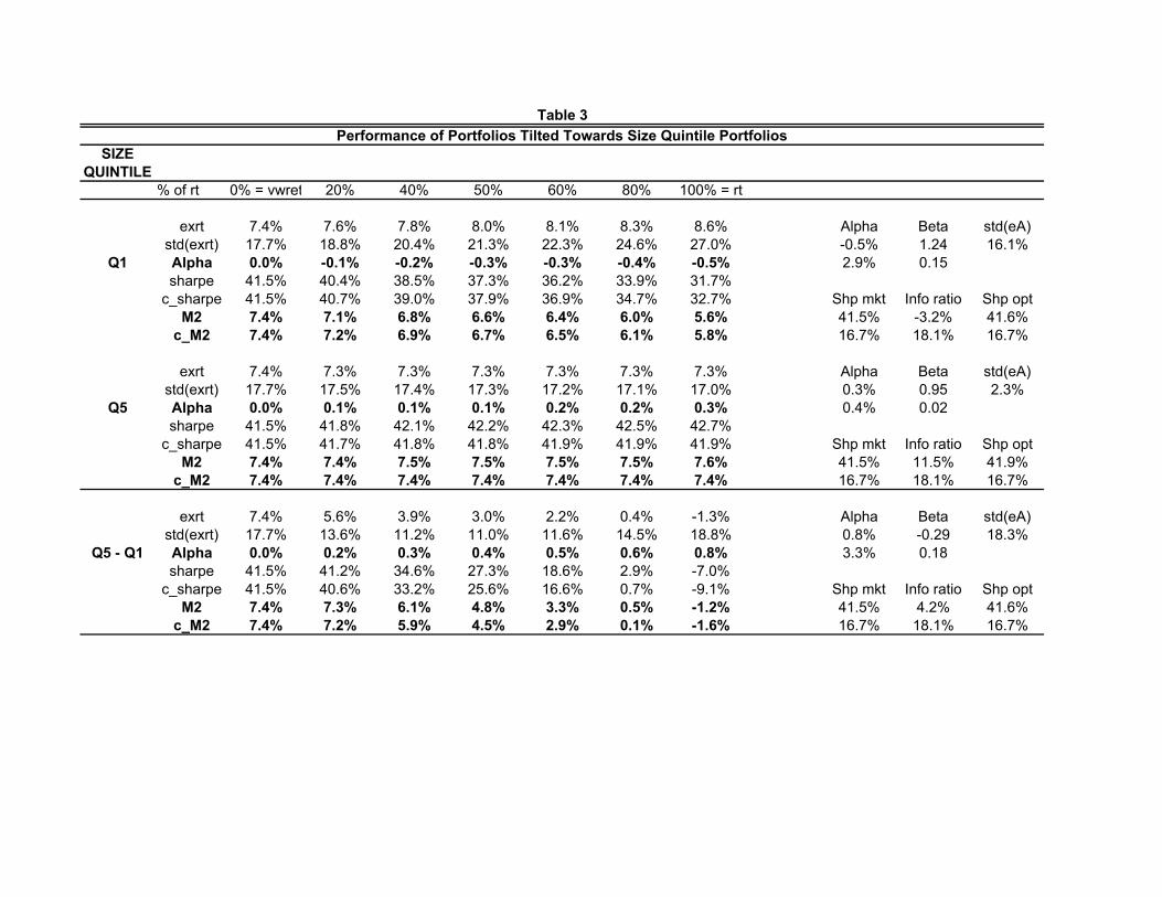
SIZE std(vw) 1/sqrt(T)QUINTILE 17.4% 0.167

% of rt 0% = vwret 20% 40% 50% 60% 80% 100% = rt

exrt 7.4% 7.6% 7.8% 8.0% 8.1% 8.3% 8.6% Alpha Beta std(eA)std(exrt) 17.7% 18.8% 20.4% 21.3% 22.3% 24.6% 27.0% -0.5% 1.24 16.1%

Q1 Alpha 0.0% -0.1% -0.2% -0.3% -0.3% -0.4% -0.5% 2.9% 0.15sharpe 41.5% 40.4% 38.5% 37.3% 36.2% 33.9% 31.7%

c_sharpe 41.5% 40.7% 39.0% 37.9% 36.9% 34.7% 32.7% Shp mkt Info ratio Shp optM2 7.4% 7.1% 6.8% 6.6% 6.4% 6.0% 5.6% 41.5% -3.2% 41.6%

c_M2 7.4% 7.2% 6.9% 6.7% 6.5% 6.1% 5.8% 16.7% 18.1% 16.7%

exrt 7.4% 7.3% 7.3% 7.3% 7.3% 7.3% 7.3% Alpha Beta std(eA)std(exrt) 17.7% 17.5% 17.4% 17.3% 17.2% 17.1% 17.0% 0.3% 0.95 2.3%

Q5 Alpha 0.0% 0.1% 0.1% 0.1% 0.2% 0.2% 0.3% 0.4% 0.02sharpe 41.5% 41.8% 42.1% 42.2% 42.3% 42.5% 42.7%

c_sharpe 41.5% 41.7% 41.8% 41.8% 41.9% 41.9% 41.9% Shp mkt Info ratio Shp optM2 7.4% 7.4% 7.5% 7.5% 7.5% 7.5% 7.6% 41.5% 11.5% 41.9%

c_M2 7.4% 7.4% 7.4% 7.4% 7.4% 7.4% 7.4% 16.7% 18.1% 16.7%

exrt 7.4% 5.6% 3.9% 3.0% 2.2% 0.4% -1.3% Alpha Beta std(eA)std(exrt) 17.7% 13.6% 11.2% 11.0% 11.6% 14.5% 18.8% 0.8% -0.29 18.3%

Q5 - Q1 Alpha 0.0% 0.2% 0.3% 0.4% 0.5% 0.6% 0.8% 3.3% 0.18sharpe 41.5% 41.2% 34.6% 27.3% 18.6% 2.9% -7.0%

c_sharpe 41.5% 40.6% 33.2% 25.6% 16.6% 0.7% -9.1% Shp mkt Info ratio Shp optM2 7.4% 7.3% 6.1% 4.8% 3.3% 0.5% -1.2% 41.5% 4.2% 41.6%

c_M2 7.4% 7.2% 5.9% 4.5% 2.9% 0.1% -1.6% 16.7% 18.1% 16.7%

Performance of Portfolios Tilted Towards Size Quintile PortfoliosTable 3

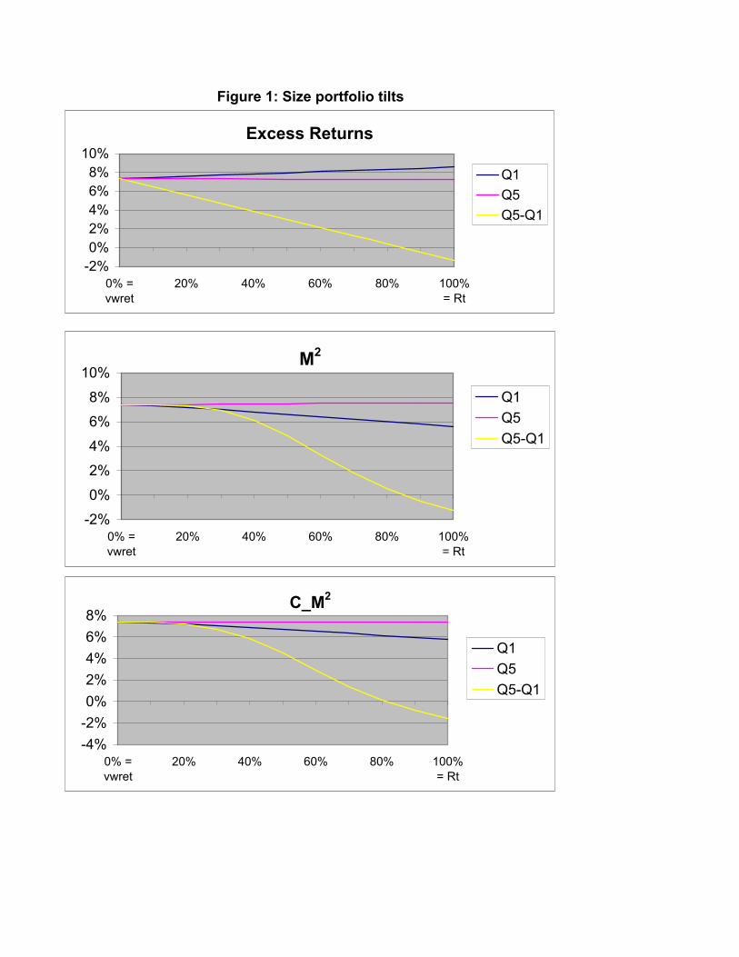
Figure 1: Size portfolio tilts

Excess Returns

-2%0%2%4%6%8%

10%

0% =vwret

20% 40% 60% 80% 100%= Rt

Q1Q5Q5-Q1

M2

-2%0%2%4%6%8%

10%

0% =vwret

20% 40% 60% 80% 100%= Rt

Q1Q5Q5-Q1

C_M2

-4%-2%0%2%4%6%8%

0% =vwret

20% 40% 60% 80% 100%= Rt

Q1Q5Q5-Q1

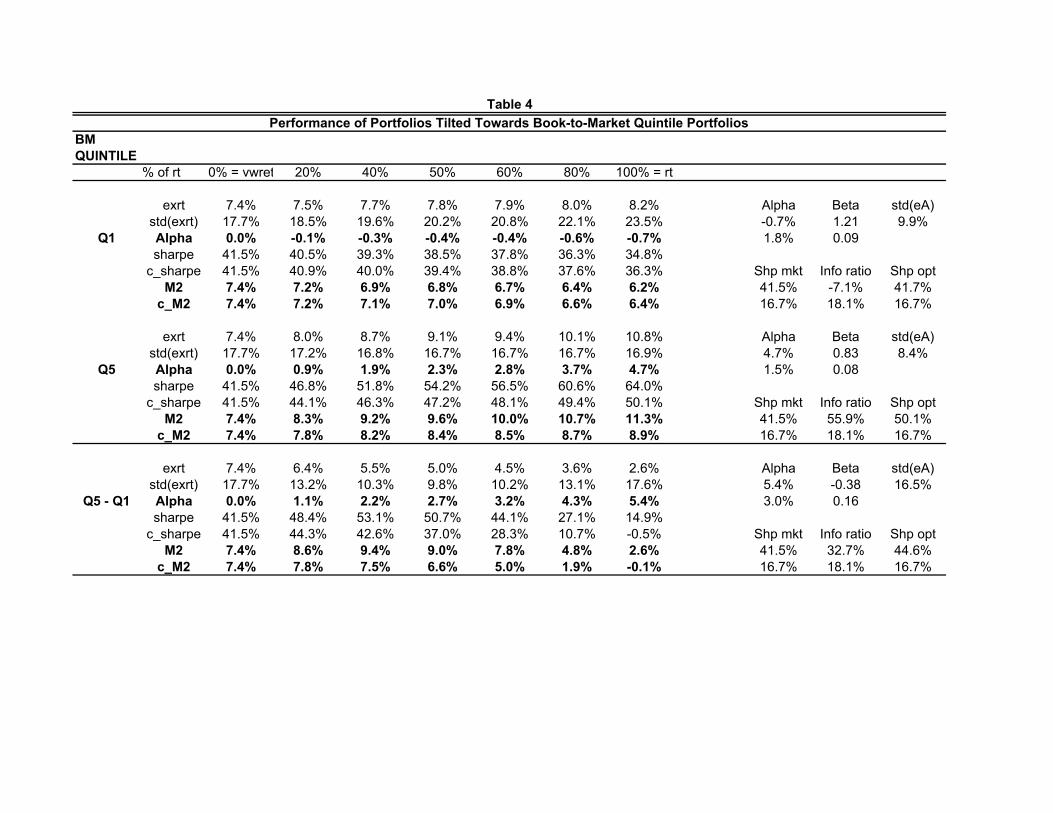
BM std(vw) 1/sqrt(T)QUINTILE 17.4% 0.167

% of rt 0% = vwret 20% 40% 50% 60% 80% 100% = rt

exrt 7.4% 7.5% 7.7% 7.8% 7.9% 8.0% 8.2% Alpha Beta std(eA)std(exrt) 17.7% 18.5% 19.6% 20.2% 20.8% 22.1% 23.5% -0.7% 1.21 9.9%

Q1 Alpha 0.0% -0.1% -0.3% -0.4% -0.4% -0.6% -0.7% 1.8% 0.09sharpe 41.5% 40.5% 39.3% 38.5% 37.8% 36.3% 34.8%

c_sharpe 41.5% 40.9% 40.0% 39.4% 38.8% 37.6% 36.3% Shp mkt Info ratio Shp optM2 7.4% 7.2% 6.9% 6.8% 6.7% 6.4% 6.2% 41.5% -7.1% 41.7%

c_M2 7.4% 7.2% 7.1% 7.0% 6.9% 6.6% 6.4% 16.7% 18.1% 16.7%

exrt 7.4% 8.0% 8.7% 9.1% 9.4% 10.1% 10.8% Alpha Beta std(eA)std(exrt) 17.7% 17.2% 16.8% 16.7% 16.7% 16.7% 16.9% 4.7% 0.83 8.4%

Q5 Alpha 0.0% 0.9% 1.9% 2.3% 2.8% 3.7% 4.7% 1.5% 0.08sharpe 41.5% 46.8% 51.8% 54.2% 56.5% 60.6% 64.0%

c_sharpe 41.5% 44.1% 46.3% 47.2% 48.1% 49.4% 50.1% Shp mkt Info ratio Shp optM2 7.4% 8.3% 9.2% 9.6% 10.0% 10.7% 11.3% 41.5% 55.9% 50.1%

c_M2 7.4% 7.8% 8.2% 8.4% 8.5% 8.7% 8.9% 16.7% 18.1% 16.7%

exrt 7.4% 6.4% 5.5% 5.0% 4.5% 3.6% 2.6% Alpha Beta std(eA)std(exrt) 17.7% 13.2% 10.3% 9.8% 10.2% 13.1% 17.6% 5.4% -0.38 16.5%

Q5 - Q1 Alpha 0.0% 1.1% 2.2% 2.7% 3.2% 4.3% 5.4% 3.0% 0.16sharpe 41.5% 48.4% 53.1% 50.7% 44.1% 27.1% 14.9%

c_sharpe 41.5% 44.3% 42.6% 37.0% 28.3% 10.7% -0.5% Shp mkt Info ratio Shp optM2 7.4% 8.6% 9.4% 9.0% 7.8% 4.8% 2.6% 41.5% 32.7% 44.6%

c_M2 7.4% 7.8% 7.5% 6.6% 5.0% 1.9% -0.1% 16.7% 18.1% 16.7%

Performance of Portfolios Tilted Towards Book-to-Market Quintile PortfoliosTable 4

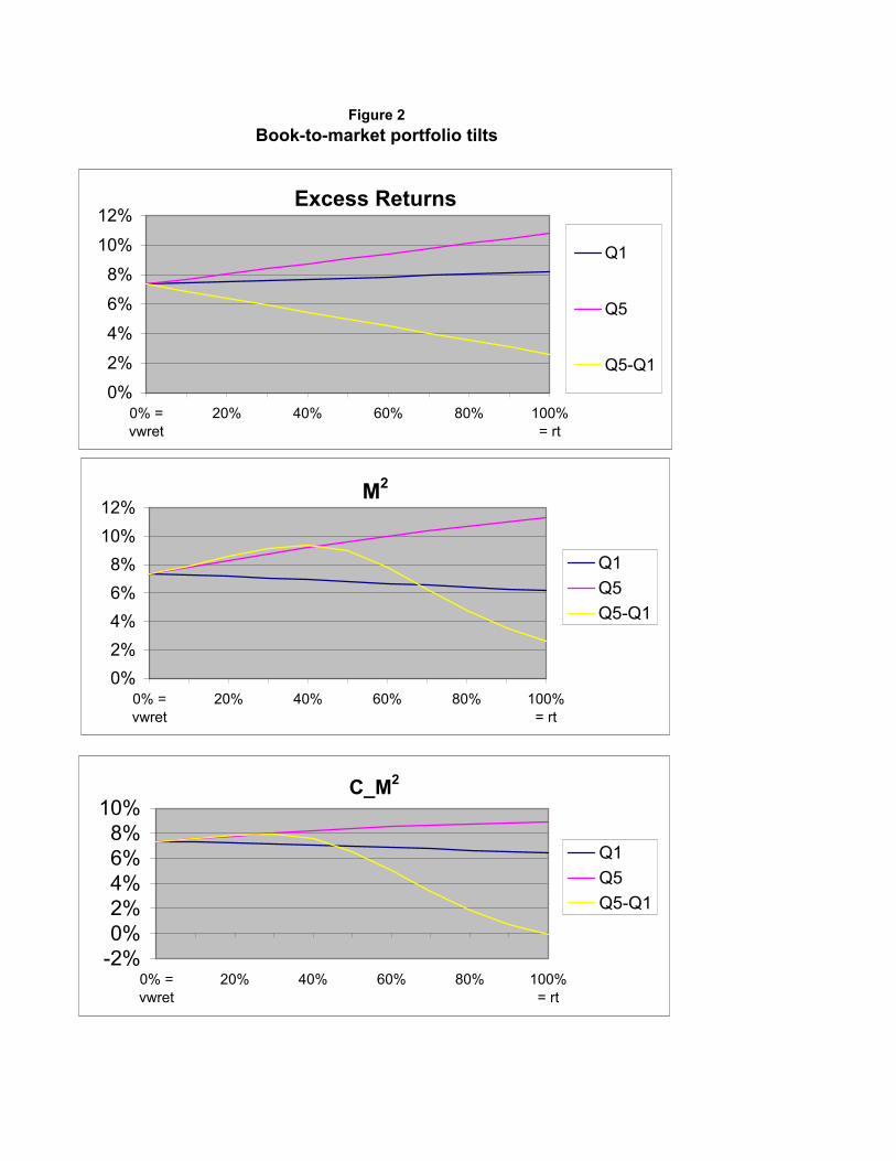
Book-to-market portfolio tiltsFigure 2

Excess Returns

0%2%4%6%8%

10%12%

0% =vwret

20% 40% 60% 80% 100%= rt

Q1

Q5

Q5-Q1

M2

0%2%4%6%8%

10%12%

0% =vwret

20% 40% 60% 80% 100%= rt

Q1Q5Q5-Q1

C_M2

-2%0%2%4%6%8%

10%

0% =vwret

20% 40% 60% 80% 100%= rt

Q1Q5Q5-Q1

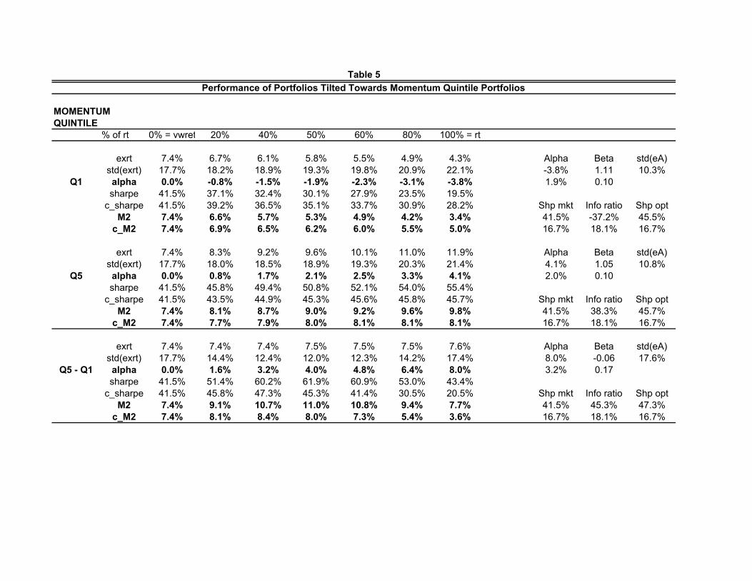
0.5MOMENTUM std(vw) 1/sqrt(T)QUINTILE 17.4% 0.167

% of rt 0% = vwret 20% 40% 50% 60% 80% 100% = rt

exrt 7.4% 6.7% 6.1% 5.8% 5.5% 4.9% 4.3% Alpha Beta std(eA)std(exrt) 17.7% 18.2% 18.9% 19.3% 19.8% 20.9% 22.1% -3.8% 1.11 10.3%

Q1 alpha 0.0% -0.8% -1.5% -1.9% -2.3% -3.1% -3.8% 1.9% 0.10sharpe 41.5% 37.1% 32.4% 30.1% 27.9% 23.5% 19.5%

c_sharpe 41.5% 39.2% 36.5% 35.1% 33.7% 30.9% 28.2% Shp mkt Info ratio Shp optM2 7.4% 6.6% 5.7% 5.3% 4.9% 4.2% 3.4% 41.5% -37.2% 45.5%

c_M2 7.4% 6.9% 6.5% 6.2% 6.0% 5.5% 5.0% 16.7% 18.1% 16.7%

exrt 7.4% 8.3% 9.2% 9.6% 10.1% 11.0% 11.9% Alpha Beta std(eA)std(exrt) 17.7% 18.0% 18.5% 18.9% 19.3% 20.3% 21.4% 4.1% 1.05 10.8%

Q5 alpha 0.0% 0.8% 1.7% 2.1% 2.5% 3.3% 4.1% 2.0% 0.10sharpe 41.5% 45.8% 49.4% 50.8% 52.1% 54.0% 55.4%

c_sharpe 41.5% 43.5% 44.9% 45.3% 45.6% 45.8% 45.7% Shp mkt Info ratio Shp optM2 7.4% 8.1% 8.7% 9.0% 9.2% 9.6% 9.8% 41.5% 38.3% 45.7%

c_M2 7.4% 7.7% 7.9% 8.0% 8.1% 8.1% 8.1% 16.7% 18.1% 16.7%

exrt 7.4% 7.4% 7.4% 7.5% 7.5% 7.5% 7.6% Alpha Beta std(eA)std(exrt) 17.7% 14.4% 12.4% 12.0% 12.3% 14.2% 17.4% 8.0% -0.06 17.6%

Q5 - Q1 alpha 0.0% 1.6% 3.2% 4.0% 4.8% 6.4% 8.0% 3.2% 0.17sharpe 41.5% 51.4% 60.2% 61.9% 60.9% 53.0% 43.4%

c_sharpe 41.5% 45.8% 47.3% 45.3% 41.4% 30.5% 20.5% Shp mkt Info ratio Shp optM2 7.4% 9.1% 10.7% 11.0% 10.8% 9.4% 7.7% 41.5% 45.3% 47.3%

c_M2 7.4% 8.1% 8.4% 8.0% 7.3% 5.4% 3.6% 16.7% 18.1% 16.7%

Performance of Portfolios Tilted Towards Momentum Quintile PortfoliosTable 5

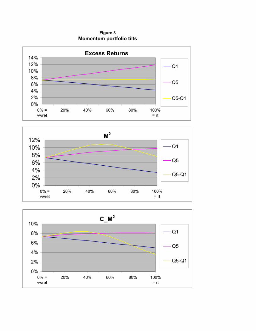
Momentum portfolio tiltsFigure 3

Excess Returns

0%2%4%6%8%

10%12%14%

0% =vwret

20% 40% 60% 80% 100%= rt

Q1

Q5

Q5-Q1

M2

0%2%4%6%8%

10%12%

0% =vwret

20% 40% 60% 80% 100%= rt

Q1

Q5

Q5-Q1

C_M2

0%

2%

4%

6%

8%

10%

0% =vwret

20% 40% 60% 80% 100%= rt

Q1

Q5

Q5-Q1

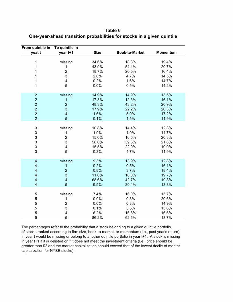
From quintile in yeat t

To quintile in year t+1 Size Book-to-Market Momentum

1 missing 34.6% 18.3% 19.4%1 1 43.9% 54.4% 20.7%1 2 18.7% 20.5% 16.4%1 3 2.6% 4.7% 14.5%1 4 0.2% 1.6% 14.7%1 5 0.0% 0.5% 14.2%

2 missing 14.9% 14.9% 13.5%2 1 17.3% 12.3% 16.1%2 2 48.3% 43.2% 20.9%2 3 17.9% 22.2% 20.3%2 4 1.6% 5.9% 17.2%2 5 0.1% 1.5% 11.9%

3 missing 10.8% 14.4% 12.3%3 1 1.9% 1.9% 14.7%3 2 15.0% 16.6% 20.3%3 3 56.6% 39.5% 21.8%3 4 15.5% 22.9% 19.0%3 5 0.2% 4.7% 11.9%

4 missing 9.3% 13.9% 12.8%4 1 0.2% 0.5% 16.1%4 2 0.8% 3.7% 18.4%4 3 11.6% 18.8% 19.7%4 4 68.6% 42.7% 19.3%4 5 9.5% 20.4% 13.8%

5 missing 7.4% 16.0% 15.7%5 1 0.0% 0.3% 20.6%5 2 0.0% 0.8% 14.9%5 3 0.1% 3.5% 13.6%5 4 6.2% 16.8% 16.6%5 5 86.2% 62.6% 18.7%

The percentages refer to the probability that a stock belonging to a given quintile portfolioof stocks ranked according to firm size, book-to-market, or momentum (I.e., past year's return) in year t would be missing or belong to another quintile portfolio in year t+1. A stock is missing in year t+1 if it is delisted or if it does not meet the investment criteria (I.e., price should be greater than $2 and the market capitalization should exceed that of the lowest decile of market capitalization for NYSE stocks).

Table 6One-year-ahead transition probabilities for stocks in a given quintile

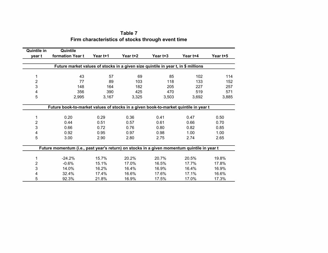
Quintile in year t

Quintile formation Year t Year t+1 Year t+2 Year t+3 Year t+4 Year t+5

1 43 57 69 85 102 114 2 77 89 103 118 133 152 3 148 164 182 205 227 257 4 356 390 425 470 519 571 5 2,995 3,167 3,325 3,503 3,692 3,885

1 0.20 0.29 0.36 0.41 0.47 0.502 0.44 0.51 0.57 0.61 0.66 0.703 0.66 0.72 0.76 0.80 0.82 0.854 0.92 0.95 0.97 0.98 1.00 1.005 3.00 2.90 2.80 2.75 2.74 2.65

1 -24.2% 15.7% 20.2% 20.7% 20.5% 19.8%2 -0.6% 15.1% 17.0% 16.5% 17.7% 17.8%3 14.0% 16.2% 16.4% 16.9% 16.4% 16.9%4 32.4% 17.4% 16.6% 17.6% 17.1% 16.6%5 92.3% 21.8% 16.9% 17.5% 17.0% 17.3%

Future market values of stocks in a given size quintile in year t, in $ millions

Future book-to-market values of stocks in a given book-to-market quintile in year t

Future momentum (i.e., past year's return) on stocks in a given momentum quintile in year t

Table 7Firm characteristics of stocks through event time

SIZE std(vw) 1/sqrt(T)QUINTILE 17.6% 0.169

% of rt 0% = vwret 20% 40% 50% 60% 80% 100% = rt

exrt 7.1% 7.6% 8.2% 8.5% 8.7% 9.3% 9.8% Alpha Beta std(eA)std(exrt) 17.9% 18.8% 20.1% 20.9% 21.8% 23.7% 25.9% 1.4% 1.18 15.3%

Q1 Alpha 0.0% 0.3% 0.6% 0.7% 0.9% 1.1% 1.4% 2.8% 0.15sharpe 39.7% 40.7% 40.7% 40.5% 40.1% 39.0% 37.9%

c_sharpe 39.7% 39.9% 39.3% 38.7% 38.1% 36.6% 35.1% Shp mkt Info ratio Shp optM2 7.1% 7.3% 7.3% 7.2% 7.2% 7.0% 6.8% 39.7% 9.4% 40.0%

c_M2 7.1% 7.1% 7.0% 6.9% 6.8% 6.6% 6.3% 16.9% 18.2% 16.9%

exrt 7.1% 7.0% 6.9% 6.9% 6.8% 6.7% 6.7% Alpha Beta std(eA)std(exrt) 17.9% 17.7% 17.5% 17.5% 17.4% 17.3% 17.2% -0.1% 0.95 3.1%

Q5 Alpha 0.0% 0.0% 0.0% 0.0% 0.0% 0.0% -0.1% 0.6% 0.03sharpe 39.7% 39.6% 39.5% 39.4% 39.3% 39.0% 38.7%

c_sharpe 39.7% 39.6% 39.5% 39.4% 39.4% 39.1% 38.9% Shp mkt Info ratio Shp optM2 7.1% 7.1% 7.1% 7.0% 7.0% 7.0% 6.9% 39.7% -1.9% 39.7%

c_M2 7.1% 7.1% 7.1% 7.1% 7.0% 7.0% 7.0% 16.9% 18.2% 16.9%

exrt 7.1% 5.0% 3.0% 2.0% 0.9% -1.1% -3.2% Alpha Beta std(eA)std(exrt) 17.9% 13.9% 11.5% 11.2% 11.6% 14.2% 18.2% -1.5% -0.23 18.0%

Q5 - Q1 alpha 0.0% -0.3% -0.6% -0.7% -0.9% -1.2% -1.5% 3.3% 0.17sharpe 39.7% 36.2% 26.1% 17.6% 8.1% -7.8% -17.4%

c_sharpe 39.7% 37.3% 28.7% 20.9% 12.0% -3.6% -13.3% Shp mkt Info ratio Shp optM2 7.1% 6.5% 4.7% 3.2% 1.5% -1.4% -3.1% 39.7% -8.3% 39.9%

c_M2 7.1% 6.7% 5.1% 3.7% 2.1% -0.6% -2.4% 16.9% 18.2% 16.9%

Table 8One Year Later Performance of Portfolios Tilted Towards Size Quintile Portfolios

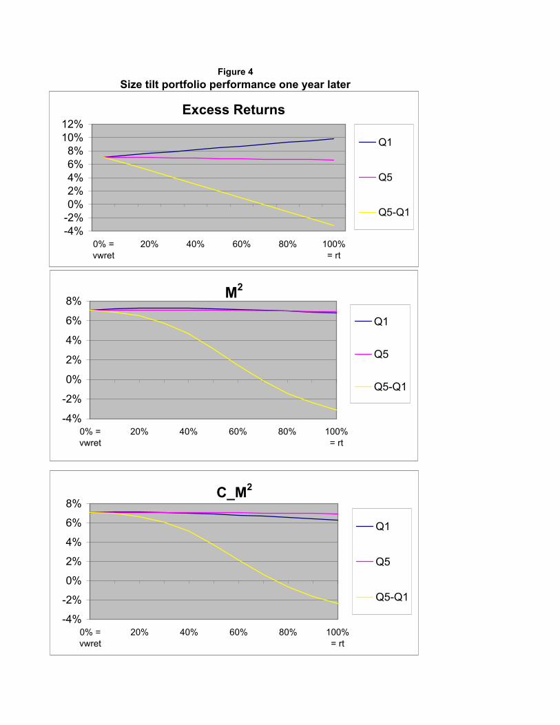
Size tilt portfolio performance one year laterFigure 4

Excess Returns

-4%-2%0%2%4%6%8%

10%12%

0% =vwret

20% 40% 60% 80% 100%= rt

Q1

Q5

Q5-Q1

M2

-4%

-2%

0%

2%

4%

6%

8%

0% =vwret

20% 40% 60% 80% 100%= rt

Q1

Q5

Q5-Q1

C_M2

-4%

-2%

0%

2%

4%

6%

8%

0% =vwret

20% 40% 60% 80% 100%= rt

Q1

Q5

Q5-Q1

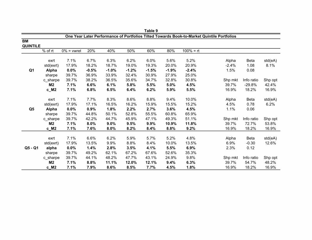
BM std(vw) 1/sqrt(T)QUINTILE 17.6% 0.169

% of rt 0% = vwret 20% 40% 50% 60% 80% 100% = rt

exrt 7.1% 6.7% 6.3% 6.2% 6.0% 5.6% 5.2% Alpha Beta std(eA)std(exrt) 17.9% 18.2% 18.7% 19.0% 19.3% 20.0% 20.9% -2.4% 1.08 8.1%

Q1 Alpha 0.0% -0.5% -1.0% -1.2% -1.5% -1.9% -2.4% 1.5% 0.08sharpe 39.7% 36.9% 33.9% 32.4% 30.9% 27.9% 25.0%

c_sharpe 39.7% 38.2% 36.5% 35.6% 34.7% 32.8% 30.8% Shp mkt Info ratio Shp optM2 7.1% 6.6% 6.1% 5.8% 5.5% 5.0% 4.5% 39.7% -29.8% 42.4%

c_M2 7.1% 6.8% 6.5% 6.4% 6.2% 5.9% 5.5% 16.9% 18.2% 16.9%

exrt 7.1% 7.7% 8.3% 8.6% 8.8% 9.4% 10.0% Alpha Beta std(eA)std(exrt) 17.9% 17.1% 16.5% 16.2% 15.9% 15.5% 15.2% 4.5% 0.78 6.2%

Q5 Alpha 0.0% 0.9% 1.8% 2.2% 2.7% 3.6% 4.5% 1.1% 0.06sharpe 39.7% 44.8% 50.1% 52.8% 55.5% 60.8% 65.9%

c_sharpe 39.7% 42.2% 44.7% 45.9% 47.1% 49.3% 51.1% Shp mkt Info ratio Shp optM2 7.1% 8.0% 9.0% 9.5% 9.9% 10.9% 11.8% 39.7% 72.7% 53.8%

c_M2 7.1% 7.6% 8.0% 8.2% 8.4% 8.8% 9.2% 16.9% 18.2% 16.9%

exrt 7.1% 6.6% 6.2% 5.9% 5.7% 5.2% 4.8% Alpha Beta std(eA)std(exrt) 17.9% 13.5% 9.9% 8.8% 8.4% 10.0% 13.5% 6.9% -0.30 12.6%

Q5 - Q1 alpha 0.0% 1.4% 2.8% 3.5% 4.1% 5.5% 6.9% 2.3% 0.12sharpe 39.7% 49.2% 62.1% 67.2% 67.6% 52.6% 35.3%

c_sharpe 39.7% 44.1% 48.2% 47.7% 43.1% 24.9% 9.8% Shp mkt Info ratio Shp optM2 7.1% 8.8% 11.1% 12.0% 12.1% 9.4% 6.3% 39.7% 54.7% 48.2%

c_M2 7.1% 7.9% 8.6% 8.5% 7.7% 4.5% 1.8% 16.9% 18.2% 16.9%

One Year Later Performance of Portfolios Tilted Towards Book-to-Market Quintile PortfoliosTable 9

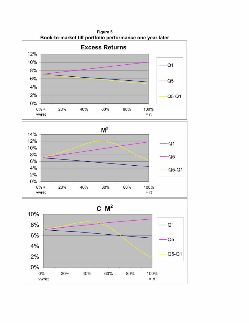
Book-to-market tilt portfolio performance one year laterFigure 5

Excess Returns

-0.05

0

0.05

0.1

0.15

0%=v

wre

t

20%

40%

60%

80%

100% =R

t

1

5

Q5-Q1

M2

-0.04-0.02

00.020.040.060.08

0%=v

wre

t

20%

40%

60%

80%

100% =R

t15Q5-Q1

C_M2

-0.04-0.02

00.020.040.060.08

0%=v

wre

t

20%

40%

60%

80%

100% =R

t

15Q5-Q1

Excess Returns

0%2%4%6%8%

10%12%

0% =vwret

20% 40% 60% 80% 100%= rt

Q1

Q5

Q5-Q1

M2

0%2%4%6%8%

10%12%14%

0% =vwret

20% 40% 60% 80% 100%= rt

Q1

Q5

Q5-Q1

C_M2

0%

2%

4%

6%

8%

10%

0% =vwret

20% 40% 60% 80% 100%= rt

Q1

Q5

Q5-Q1

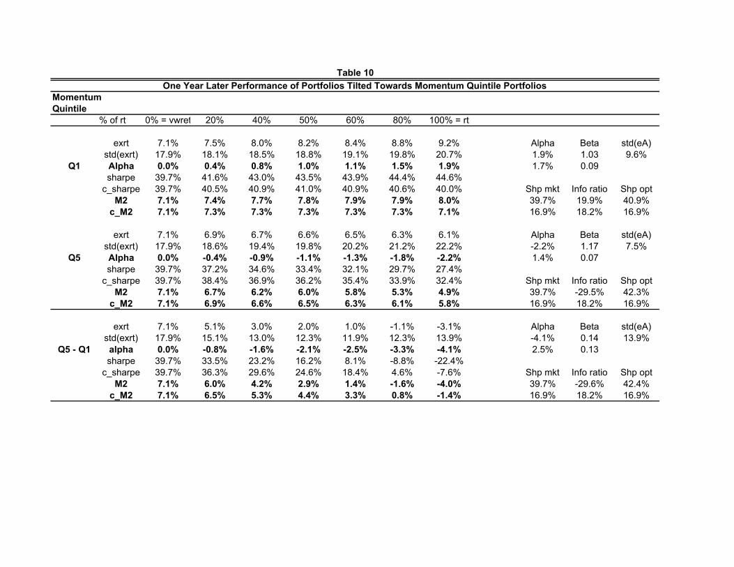
Momentum std(vw) 1/sqrt(T)Quintile 17.6% 0.169

% of rt 0% = vwret 20% 40% 50% 60% 80% 100% = rt

exrt 7.1% 7.5% 8.0% 8.2% 8.4% 8.8% 9.2% Alpha Beta std(eA)std(exrt) 17.9% 18.1% 18.5% 18.8% 19.1% 19.8% 20.7% 1.9% 1.03 9.6%

Q1 Alpha 0.0% 0.4% 0.8% 1.0% 1.1% 1.5% 1.9% 1.7% 0.09sharpe 39.7% 41.6% 43.0% 43.5% 43.9% 44.4% 44.6%

c_sharpe 39.7% 40.5% 40.9% 41.0% 40.9% 40.6% 40.0% Shp mkt Info ratio Shp optM2 7.1% 7.4% 7.7% 7.8% 7.9% 7.9% 8.0% 39.7% 19.9% 40.9%

c_M2 7.1% 7.3% 7.3% 7.3% 7.3% 7.3% 7.1% 16.9% 18.2% 16.9%

exrt 7.1% 6.9% 6.7% 6.6% 6.5% 6.3% 6.1% Alpha Beta std(eA)std(exrt) 17.9% 18.6% 19.4% 19.8% 20.2% 21.2% 22.2% -2.2% 1.17 7.5%

Q5 Alpha 0.0% -0.4% -0.9% -1.1% -1.3% -1.8% -2.2% 1.4% 0.07sharpe 39.7% 37.2% 34.6% 33.4% 32.1% 29.7% 27.4%

c_sharpe 39.7% 38.4% 36.9% 36.2% 35.4% 33.9% 32.4% Shp mkt Info ratio Shp optM2 7.1% 6.7% 6.2% 6.0% 5.8% 5.3% 4.9% 39.7% -29.5% 42.3%

c_M2 7.1% 6.9% 6.6% 6.5% 6.3% 6.1% 5.8% 16.9% 18.2% 16.9%

exrt 7.1% 5.1% 3.0% 2.0% 1.0% -1.1% -3.1% Alpha Beta std(eA)std(exrt) 17.9% 15.1% 13.0% 12.3% 11.9% 12.3% 13.9% -4.1% 0.14 13.9%

Q5 - Q1 alpha 0.0% -0.8% -1.6% -2.1% -2.5% -3.3% -4.1% 2.5% 0.13sharpe 39.7% 33.5% 23.2% 16.2% 8.1% -8.8% -22.4%

c_sharpe 39.7% 36.3% 29.6% 24.6% 18.4% 4.6% -7.6% Shp mkt Info ratio Shp optM2 7.1% 6.0% 4.2% 2.9% 1.4% -1.6% -4.0% 39.7% -29.6% 42.4%

c_M2 7.1% 6.5% 5.3% 4.4% 3.3% 0.8% -1.4% 16.9% 18.2% 16.9%

One Year Later Performance of Portfolios Tilted Towards Momentum Quintile PortfoliosTable 10

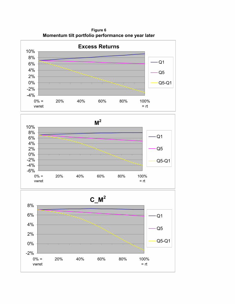
Momentum tilt portfolio performance one year laterFigure 6

Excess Returns

-4%-2%0%2%4%6%8%

10%

0% =vwret

20% 40% 60% 80% 100%= rt

Q1

Q5

Q5-Q1

M2

-6%-4%-2%0%2%4%6%8%

10%

0% =vwret

20% 40% 60% 80% 100%= rt

Q1

Q5

Q5-Q1

C_M2

-2%

0%

2%

4%

6%

8%

0% =vwret

20% 40% 60% 80% 100%= rt

Q1

Q5

Q5-Q1

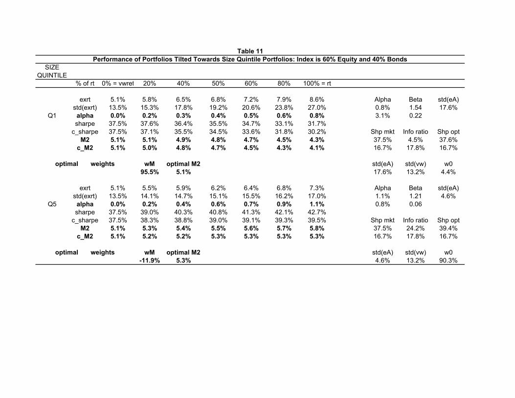
SIZE std(vw) 1/sqrt(T)QUINTILE 13.2% 0.167

% of rt 0% = vwret 20% 40% 50% 60% 80% 100% = rt

exrt 5.1% 5.8% 6.5% 6.8% 7.2% 7.9% 8.6% Alpha Beta std(eA)std(exrt) 13.5% 15.3% 17.8% 19.2% 20.6% 23.8% 27.0% 0.8% 1.54 17.6%

Q1 alpha 0.0% 0.2% 0.3% 0.4% 0.5% 0.6% 0.8% 3.1% 0.22sharpe 37.5% 37.6% 36.4% 35.5% 34.7% 33.1% 31.7%

c_sharpe 37.5% 37.1% 35.5% 34.5% 33.6% 31.8% 30.2% Shp mkt Info ratio Shp optM2 5.1% 5.1% 4.9% 4.8% 4.7% 4.5% 4.3% 37.5% 4.5% 37.6%

c_M2 5.1% 5.0% 4.8% 4.7% 4.5% 4.3% 4.1% 16.7% 17.8% 16.7%

optimal TB weights wM optimal M2 std(eA) std(vw) w095.5% 5.1% 17.6% 13.2% 4.4%

exrt 5.1% 5.5% 5.9% 6.2% 6.4% 6.8% 7.3% Alpha Beta std(eA)std(exrt) 13.5% 14.1% 14.7% 15.1% 15.5% 16.2% 17.0% 1.1% 1.21 4.6%

Q5 alpha 0.0% 0.2% 0.4% 0.6% 0.7% 0.9% 1.1% 0.8% 0.06sharpe 37.5% 39.0% 40.3% 40.8% 41.3% 42.1% 42.7%

c_sharpe 37.5% 38.3% 38.8% 39.0% 39.1% 39.3% 39.5% Shp mkt Info ratio Shp optM2 5.1% 5.3% 5.4% 5.5% 5.6% 5.7% 5.8% 37.5% 24.2% 39.4%

c_M2 5.1% 5.2% 5.2% 5.3% 5.3% 5.3% 5.3% 16.7% 17.8% 16.7%

optimal TB weights wM optimal M2 std(eA) std(vw) w0-11.9% 5.3% 4.6% 13.2% 90.3%

Table 11Performance of Portfolios Tilted Towards Size Quintile Portfolios: Index is 60% Equity and 40% Bonds

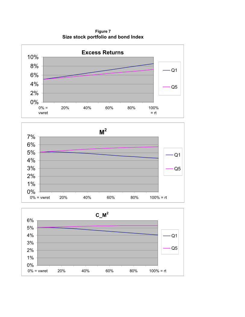
Size stock portfolio and bond IndexFigure 7

Excess Returns

0%2%4%6%8%

10%

0% =vwret

20% 40% 60% 80% 100%= rt

Q1

Q5

M2

0%1%2%3%4%5%6%7%

0% = vwret 20% 40% 60% 80% 100% = rt

Q1

Q5

C_M2

0%1%2%3%4%5%6%

0% = vwret 20% 40% 60% 80% 100% = rt

Q1

Q5

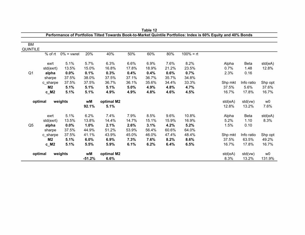
BM std(vw) 1/sqrt(T)QUINTILE 13.2% 0.167

% of rt 0% = vwret 20% 40% 50% 60% 80% 100% = rt

exrt 5.1% 5.7% 6.3% 6.6% 6.9% 7.6% 8.2% Alpha Beta std(eA)std(exrt) 13.5% 15.0% 16.8% 17.8% 18.9% 21.2% 23.5% 0.7% 1.48 12.8%

Q1 alpha 0.0% 0.1% 0.3% 0.4% 0.4% 0.6% 0.7% 2.3% 0.16sharpe 37.5% 38.0% 37.5% 37.1% 36.7% 35.7% 34.8%

c_sharpe 37.5% 37.5% 36.7% 36.1% 35.6% 34.4% 33.3% Shp mkt Info ratio Shp optM2 5.1% 5.1% 5.1% 5.0% 4.9% 4.8% 4.7% 37.5% 5.6% 37.6%

c_M2 5.1% 5.1% 4.9% 4.9% 4.8% 4.6% 4.5% 16.7% 17.8% 16.7%

optimal TB weights wM optimal M2 std(eA) std(vw) w092.1% 5.1% 12.8% 13.2% 7.6%

exrt 5.1% 6.2% 7.4% 7.9% 8.5% 9.6% 10.8% Alpha Beta std(eA)std(exrt) 13.5% 13.8% 14.4% 14.7% 15.1% 15.9% 16.9% 5.2% 1.10 8.3%

Q5 alpha 0.0% 1.0% 2.1% 2.6% 3.1% 4.2% 5.2% 1.5% 0.10sharpe 37.5% 44.9% 51.2% 53.9% 56.4% 60.6% 64.0%

c_sharpe 37.5% 41.1% 43.9% 45.0% 46.0% 47.4% 48.4% Shp mkt Info ratio Shp optM2 5.1% 6.0% 6.9% 7.3% 7.6% 8.2% 8.6% 37.5% 63.5% 49.2%

c_M2 5.1% 5.5% 5.9% 6.1% 6.2% 6.4% 6.5% 16.7% 17.8% 16.7%

optimal TB weights wM optimal M2 std(eA) std(vw) w0-51.2% 6.6% 8.3% 13.2% 131.9%

Table 12Performance of Portfolios Tilted Towards Book-to-Market Quintile Portfolios: Index is 60% Equity and 40% Bonds

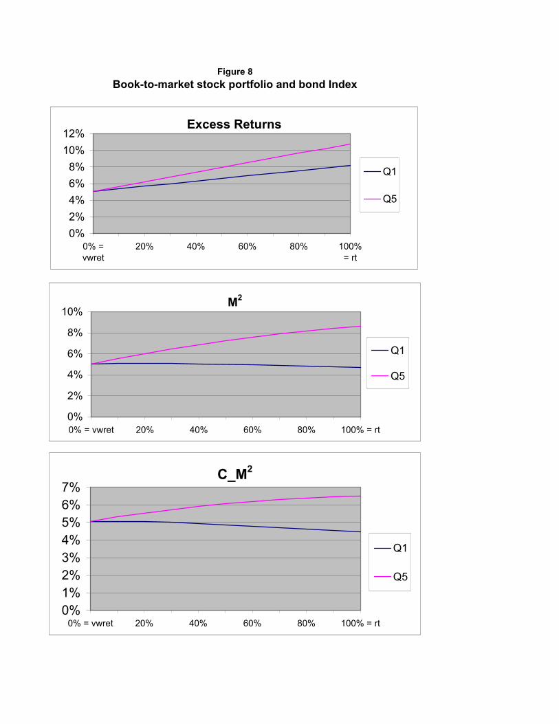
Book-to-market stock portfolio and bond IndexFigure 8

Excess Returns

0%2%4%6%8%

10%12%

0% =vwret

20% 40% 60% 80% 100%= rt

Q1

Q5

M2

0%

2%

4%

6%

8%

10%

0% = vwret 20% 40% 60% 80% 100% = rt

Q1

Q5

C_M2

0%1%2%3%4%5%6%7%

0% = vwret 20% 40% 60% 80% 100% = rt

Q1

Q5

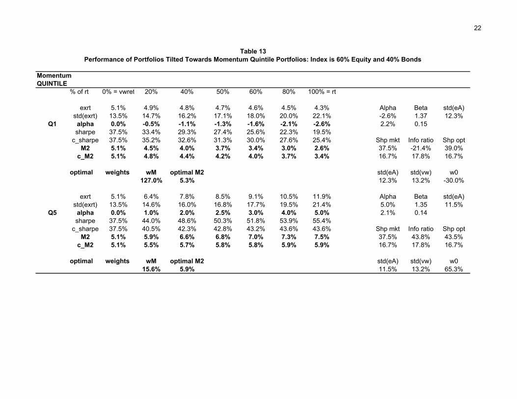
22

Momentum std(vw) 1/sqrt(T)QUINTILE 13.2% 0.166667

% of rt 0% = vwret 20% 40% 50% 60% 80% 100% = rt

exrt 5.1% 4.9% 4.8% 4.7% 4.6% 4.5% 4.3% Alpha Beta std(eA)std(exrt) 13.5% 14.7% 16.2% 17.1% 18.0% 20.0% 22.1% -2.6% 1.37 12.3%

Q1 alpha 0.0% -0.5% -1.1% -1.3% -1.6% -2.1% -2.6% 2.2% 0.15sharpe 37.5% 33.4% 29.3% 27.4% 25.6% 22.3% 19.5%

c_sharpe 37.5% 35.2% 32.6% 31.3% 30.0% 27.6% 25.4% Shp mkt Info ratio Shp optM2 5.1% 4.5% 4.0% 3.7% 3.4% 3.0% 2.6% 37.5% -21.4% 39.0%

c_M2 5.1% 4.8% 4.4% 4.2% 4.0% 3.7% 3.4% 16.7% 17.8% 16.7%

optimal TB weights wM optimal M2 std(eA) std(vw) w0127.0% 5.3% 12.3% 13.2% -30.0%

exrt 5.1% 6.4% 7.8% 8.5% 9.1% 10.5% 11.9% Alpha Beta std(eA)std(exrt) 13.5% 14.6% 16.0% 16.8% 17.7% 19.5% 21.4% 5.0% 1.35 11.5%

Q5 alpha 0.0% 1.0% 2.0% 2.5% 3.0% 4.0% 5.0% 2.1% 0.14sharpe 37.5% 44.0% 48.6% 50.3% 51.8% 53.9% 55.4%

c_sharpe 37.5% 40.5% 42.3% 42.8% 43.2% 43.6% 43.6% Shp mkt Info ratio Shp optM2 5.1% 5.9% 6.6% 6.8% 7.0% 7.3% 7.5% 37.5% 43.8% 43.5%

c_M2 5.1% 5.5% 5.7% 5.8% 5.8% 5.9% 5.9% 16.7% 17.8% 16.7%

optimal TB weights wM optimal M2 std(eA) std(vw) w015.6% 5.9% 11.5% 13.2% 65.3%

Table 13Performance of Portfolios Tilted Towards Momentum Quintile Portfolios: Index is 60% Equity and 40% Bonds

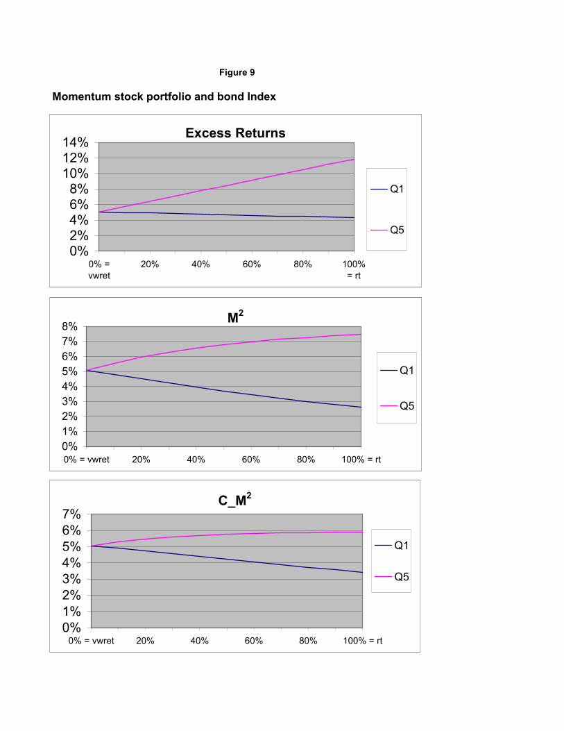
Momentum stock portfolio and bond Index

Figure 9

Excess Returns

0%2%4%6%8%

10%12%14%

0% =vwret

20% 40% 60% 80% 100%= rt

Q1

Q5

M2

0%1%2%3%4%5%6%7%8%

0% = vwret 20% 40% 60% 80% 100% = rt

Q1

Q5

C_M2

0%1%2%3%4%5%6%7%

0% = vwret 20% 40% 60% 80% 100% = rt

Q1

Q5

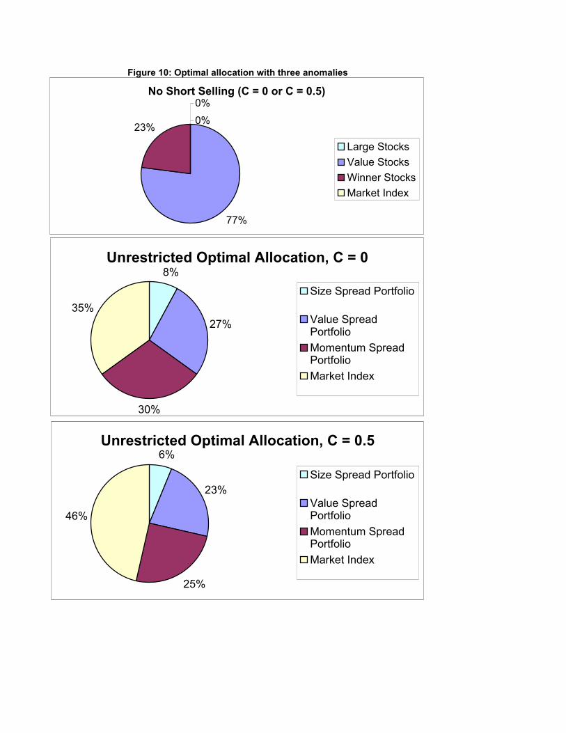
No Short Selling No Short SellingC=0 C=0.5Large Stocks 0% 0%Value Stocks 77% 77%Winner Stocks 23% 23%Market Index 0% 0%

Unrestricted Optimal Allocation c = 0Size Spread Portfolio 8%Value Spread Portfolio 27%Momentum Spread Portfolio 30%Market Index 35%

Unrestricted Optimal Allocation c = 0.5Size Spread Portfolio 5%Value Spread Portfolio 20%Momentum Spread Portfolio 22%Market Index 41%

Figure 10: Optimal allocation with three anomalies

No Short Selling (C = 0 or C = 0.5)

0%

77%

23%

0%

Large StocksValue StocksWinner StocksMarket Index

Unrestricted Optimal Allocation, C = 08%

27%

30%

35%Size Spread Portfolio

Value SpreadPortfolioMomentum SpreadPortfolioMarket Index

Unrestricted Optimal Allocation, C = 0.56%

23%

25%

46%

Size Spread Portfolio

Value SpreadPortfolioMomentum SpreadPortfolioMarket Index