Embed Size (px)
Citation preview
Assessor’s Ratio Procedures
Manual
2017

Oregon Department of Revenue Ratio Study Procedures 2017
Preface
Purpose of the Ratio Manual
The purpose of the Oregon Department of Revenue Assessor’s Certified Ratio Study Procedures
Manual is to provide guidance and instruction to county assessors and analysts to complete ratio
studies that result in an Assessor’s Certified Ratio Study report complying with Oregon Revised
Statutes (ORS) 309.200 and Oregon Administrative Rule (OAR) 150-309-0230, 150-309-0240,
150-309-0240.
Scope and Limitation of the Ratio Manual
This technical manual outlines processes and procedures for achieving consistent and verifiable
ratio studies. Additionally, the manual provides a standardized structure to be utilized when
reporting ratio study findings. Authority and limitations for development of the manual is
provided by Oregon statutes and rules. The International Association of Assessing Officers
(IAAO) Standard on Ratio Studies (2013) was consulted as a guiding reference.
The manual is a result of collaborative efforts between the Department of Revenue and county
assessors, managers, and analysts, and is intended to be modified and updated on an ongoing
basis.

Oregon Department of Revenue Ratio Study Procedures 2017 i
Ratio Procedures Manual
Table of Contents
PREFACE
INTRODUCTION:
BASIC STEPS, AND TIMELINE SECTION 1 Definitions 1-1
Purpose of the Assessor’s Certified Ratio Study Report 1-2
The Ratio Study Manual 1-3
Users of the Assessor’s Certified Ratio Study Reports 1-4
Basic Steps to Complete a Ratio Study 1-6
Timeline 1-7
PROPERTY CLASSIFICATION SECTION 2
Basic Property Classes 2-2
Multi-Account Sales 2-8
Machinery and Equipment 2-8
SALES DATA COLLECTION AND STANDARD DATA FORMAT SECTION 3
Sales Data Year 3-1
Market Data Sources 3-1
Sales Database 3-2
Property Sale Identification 3-3
Multi-Account Sales 3-3
Standard Data Format 3-3
Database Fields 3-3
INVESTIGATING SALE TRANSACTIONS SECTION 4
Sales Confirmation and Verification 4-1
Methods of Confirmation and Verification 4-2
Questionnaire Letter 4-2
Telephone Contact 4-3
Email or Internet Digital Form 4-3
Field Inspection 4-3
An Exception to Typical Confirmation Practices 4-4
Oregon Department of Revenue Ratio Study Procedures 2017 ii
Sale Adjustments and Qualification 4-4
Adjustments to Identify and Consider 4-4
Multi-Account Sales 4-5
General Acceptance of Sales 4-5
Identifying Unusable Sales 4-5
Sales with Special Conditions 4-6
Condition Codes (IAAO Reason Code) 4-8
Sales Data Condition (Reject or Reason Codes (DOR) 4-9
Sample Sales Cover Letters and Questionnaires 4-11
DATA ORGANIZATION:
RATIO CALCULATION, OUTLIERS, &TRIMMING SECTION 5 Ratio Calculation 5-1
Scatter Diagram 5-3
Outliers 5-4
Method: A Trimmed Mean 5-5
Trimming Limits 5-5
Method: Interquartile Range Trimming 5-7
Trimming Limits Specific to IQR 5-11
Trimming Recap 5-11
BASIC RATIO STATISTICS SECTION 6
Introduction 6-1
Central Tendencies (Ratio Indications) 6-2
Median 6-3
Mean 6-5
Weighted Mean 6-6
Other Measures of Central Tendency to Consider 6-8
Geometric Mean 6-8
Mode 6-9
ANALYSIS: CHANGE IN MARKET CONDITIONS OVER TIME SECTION 7
Introduction 7-1
Types of Trends 7-2
Examining Market Trends 7-3
Ratio Analysis: Diagramming Sales Ratio and Adding a Trend Line 7-5

Oregon Department of Revenue Ratio Study Procedures 2017 iii
Determining the Rate of Change over Time 7-7
Ratio Analysis: Direct Calculation Applied on an Annual Basis 7-7
Ratio Analysis: Direct Calculation on Monthly or Quarterly Basis 7-12
Ratio Analysis: Mid-point 7-16
Direct Sales Analysis 7-19
Double Sales 7-20
Paired Sales 7-21
ANALYSIS: MARKET AREA STRATIFICATION SECTION 8
History of Stratification in Oregon Property Mass Appraisal Valuation 8-1
Stratification 8-1
Neighborhood 8-2
Neighborhood Codes 8-4
Market Area 8-4
Combining Neighborhoods in Market (Study) Areas 8-5
Redefining Market Areas 8-7
Conclusion 8-8
ANALYZING DATA FOR SAMPLE BIAS,
MEASURES OF UNIFORMITY & RELIABILITY SECTION 9
Sample Bias 9-1
Testing for Bias 9-2
Ratio Distribution 9-3
Common Ratio Distributions 9-4
Construct a Histogram 9-6
Measures of Appraisal Uniformity 9-8
Average Absolute Deviation (AAD) 9-8
Coefficient of Dispersion (COD) 9-9
COD Standards 9-10
Standard Deviation 9-11
Sample Distribution 9-12
Coefficient of Variation (COV) 9-14
Price Related Differential (PRD) 9-14
Measuring Regressivity and Progressivity 9-15
Weighting 9-17
Measures of Reliability 9-24
Oregon Department of Revenue Ratio Study Procedures 2017 iv
RECALCULATION TRENDING AND ADDITIONAL STUDIES SECTION 10
Recalculation 10-1
Ratio Study Analysis Before Adjustment of Roll Values (Before Ratio) 10-3
Recalculation Process 10-3
Ratio Study Analysis After Adjustment of Roll Values (After Ratio) 10-4
Supplemental Studies 10-4
Straddle Study 10-5
Appraisal Ratio Studies 10-5
PREPARING AND ASSEMBLING THE RATIO STUDY REPORT SECTION 11
STATUTES AND RULES SECTION 12
GLOSSARY

Oregon Department of Revenue Ratio Study Procedures 2017 1-1
SECTION 1
INTRODUCTION,
BASIC STEPS, AND TIMELINE
County assessors are responsible for managing estimates of property values and annually
developing new assessment and tax rolls. Assessment roll value changes are a direct result of
research conducted by the assessor’s office employing mass appraisal techniques to maintain
uniformity and equity.
Real estate prices continually fluctuate throughout the year. Oregon Revised Statutes (ORS)
mandate assessors track and measure the real estate market in order to maintain 100 percent of
real market value (RMV) as of the January 1 assessment date. To demonstrate compliance has
been achieved, assessors are required by ORS 309.200 to annually complete ratio studies and
publish the Assessor’s Certified Ratio Study report. With the knowledge attained while
completing the ratio study, the assessor can identify appraisal priorities.
The report assists the Department of Revenue (DOR) in fulfilling the role of general supervision
and control over the statewide system of property taxation provided in ORS 306.115(1). The
department reviews the counties’ valuation programs to verify standards are met and to measure
the health of the statewide valuation system.
Definitions
Assessment Date:
Oregon Revised Statute (ORS) 308.210 Assessing property; record as assessment roll; changes in ownership or description of real property and manufactured structures assessed as personal property.
(1) The assessor shall proceed each year to assess the value of all taxable property within the county, except property that by law is to be otherwise assessed. The assessor shall maintain a full and complete record of the assessment of the taxable property for each year as of January 1, at 1:00 a.m. of the assessment year, in the manner set forth in ORS 308.215. Such record shall constitute the assessment roll of the county for the year.
Oregon Department of Revenue Ratio Study Procedures 2017 1-2
Ratio Study:
Oregon Administrative Rule (OAR) 150-309-0230 (4) Appraisal ratio study is a statistical compilation of appraisal ratios for a representative group of properties in the county randomly selected on a property class basis to produce an indication of the ratio of the prior year's real market value to the current year's real market value for all taxable properties in a particular class of property within the county, in a particular class of property within an appraisal area, or in a particular class of property within a market area.
(12) Ratio study is a study which estimates: (a) The percentage relationship between the total prior year's real market value of each class of taxable property on the prior assessment roll and the total current real market value of the same properties in each class on the current assessment roll; and (b) The percentage relationship between the total prior year's real market value of each class of taxable property on the prior assessment roll and the total current real market value of the same properties in each class on the current assessment roll within each appraisal area, or market area.
(13) Sales ratio is the percentage relationship between the real market value for the prior assessment year and the selling price for a particular property.
Specifically, RMV divided by the sale price results in a sales ratio.
(RMV / Sale Price = Sales Ratio)
Purpose of the Assessor’s Certified Ratio Study Report
The annual studies and ratio report:
Provides supportable conclusions for adjusting roll values to arrive at 100 percent of
RMV in compliance with ORS 308.232
Fulfills the assessor’s requirement set forth in ORS 309.200(1)(2)(3) to supply a report
providing conclusions relating to market value to the clerk of the Board of Property Tax
Appeals (BoPTA)
Establishes a basis for testing county valuation programs. It creates a source of data that
allows the county assessor and the Department of Revenue to measure results of the
assessment programs
Oregon Department of Revenue Ratio Study Procedures 2017 1-3
The study is a primary management tool as stated by the International Association of Assessing
Officers (IAAO):
Local jurisdictions should use ratio studies as a primary mass appraisal testing procedure and their most important performance analysis tool. Ratio studies provide a means for testing and evaluating mass appraisal valuation models to ensure the value estimates meet attainable standards of accuracy. (IAAO Standard on Ratio Studies, 2013, pg 8)
The Ratio Study Manual
The DOR Assessor’s Certified Ratio Study Procedures Manual outlines a systematic approach to
preparing and reporting ratio studies. The purpose of the ratio manual is to provide county
assessors and analysts with procedures for developing ratio studies as required by ORS 309.200.
The department must approve any deviation from the procedures set out in this manual OAR
150-309-0250(2). The manual covers these topics:
Collecting sales data
Classifying and sorting sales according to property class/use
Confirming and verifying market transactions; investigating outliers, researching
anomalies
Calculating change in market conditions over time
Identifying patterns in market areas
Calculating ratios indicating a measurable difference between RMV and market sales
Applying statistical methods of measurement
Assembling required elements of an Assessor’s Certified Ratio Study report
The ratio manual provides guidance to assessors and analysts in fulfilling the following
responsibilities:
Researching and verifying market transactions
Preparing and adjusting sales to use in the ratio study
Sorting sales according to property class
Calculating ratios
Analyzing sales to identify patterns and anomalies
Applying statistical methods to develop market related conclusions
Oregon Department of Revenue Ratio Study Procedures 2017 1-4
Creating an official document demonstrating report conclusions for a specified date
Communicating this information to assessors, appraisers, taxpayers, and public officials
Certification of the Assessor’s Certified Ratio Study confirms the report meets statutory
requirements. When the ratio study report is completed, it is submitted to the Oregon Department
of Revenue and is available for public review.
The Assessor’s Certified Ratio Study reports are used by:
Assessors demonstrate compliance with statute by developing a supportable annual ratio study
which can then be used to develop the required valuation plan. As a management tool, the
assessor can ensure adequate staff and resources are available to meet assessment obligations.
The assessor’s staff may present information from the Assessor’s Certified Ratio Study report as
a resource and reference document to the county BoPTA members in support of roll real market
values.
The Board of Property Tax Appeals utilizes the ratio study in their decision making process
regarding appeals brought before the Board. ORS 309.200(1)(2)(3) states this study shall be filed
with the Clerk of the Board no later than October 15 of each year; this allows board members the
opportunity to review the study’s conclusions before convening in February when appeal reviews
begin.
A copy of the report is required to be filed with the Department of Revenue who examines the
assessor’s ratio programs and ratio reports to: measure compliance with statutes, ensure equitable
assessment levels, and monitor county valuation programs for determination of appropriate
valuation results.
Appraisers use sales files and ratio studies together as key elements in the management of
valuation areas. For each area, pertinent data can be extracted from the sales file and analyzed.
Appraisers determine current real market value levels by property class, review extreme ratios
Oregon Department of Revenue Ratio Study Procedures 2017 1-5
for possible errors in appraisals, and identify the need for further stratification of the sales data to
determine whether there are separate market influences within the market area being measured.
During setup, the Assessor’s Certified Ratio Study report can supply a time trend adjustment and
provide support to the analysis. Corroborating outcomes increase the reliability of appraisal
conclusions of real market value.
The Department of Justice and Tax Courts may consult county ratio studies as established
reference documentation in support of local and statewide valuation appeals.
County governing bodies refer to the Assessor’s Certified Ratio Study report when establishing
potential funding levels and allowances for community services dependent upon local funding
(i.e., police, fire, improvement districts, etc.). By statute, the department’s annual ratio review
findings and recommendation letters sent to each assessor are forwarded to the county governing
body.
The state Legislature uses county ratio studies to evaluate statewide performance of assessment
programs.
Taxpayers can reference this resource document regarding residential, commercial, and
industrial valuation. The report supplies information regarding applied trends, market activity,
and sales data.
Oregon Department of Revenue Ratio Study Procedures 2017 1-6
Basic Steps to Complete a Ratio Study
1. Collect sales for the time period January 1 through December 31.
2. Confirm and verify sales for analysis.
3. Provide the sales database, including all rejected sales, to the Department of Revenue, when requested, under its supervisory responsibility and authority per ORS 306.115.
4. Check outlier ratios for needed additional analysis before inclusion in the array.
5. Create a sales file containing only qualified, usable sales.
6. Conduct a sales time trend analysis to determine if adjustments for changes in market conditions over time are appropriate.
7. Apply indicated time trends to adjust sales or ratios to the assessment date. Calculate measures of central tendency and select the most representative one before adjusting prior year’s roll values.
8. Analyze each sales array; address arrays that may need supplemental studies (e.g., multi–years, similar class combined, etc.). Calculate central tendencies and select the most representative one; compute an adjustment factor. Test results.
9. Prepare and assemble the ratio study report.
10. Submit a copy of the Assessor’s Certified Ratio Study report with the DOR no later than July 1 per OAR 150-309-0250.
a. The DOR will examine each study and submit written recommendations or orders prior to September 1 to each assessor and county governing body per ORS 309.203.
b. The assessor applies the adjustment factors to the real market values on the roll as recommended by DOR.
11. A certified copy of the Assessor’s Certified Ratio Study report must be filed with the Clerk of the Board of Property Tax Appeals per ORS 309.200(3) no later than October 15.
Oregon Department of Revenue Ratio Study Procedures 2017 1-7
Timeline
January 1: The sales collection year begins January 1 and ends December 31. Sales information is collected, confirmed, sorted, and determined to be usable or unusable, and condition is coded and entered into the sales file. Periodically, the volume of sales data is checked and a plan is developed for additional studies, if necessary.
The ratio study year begins immediately following the sales collection year (for example: the sales collection year of January 1, 2014 through December 31, 2014 is for the January 1, 2015 ratio study year), and continues until the Assessor’s Certified Ratio Study report is complete. Sales analysis may be started earlier than the January 1 assessment date. Some important dates to consider are as follows:
February 15: All sales should be entered into the database.
On or before Deadline to file a certified copy of the ratio study with the Department of July 1: Revenue, Property Tax Division, or request an extension in writing.
August 1: Last date to submit a report if an extension has been granted.
On or before The department provides written findings and recommendations September 1: to the assessor. A copy is sent to the county governing body. The department
notifies assessors if assessment levels are in jeopardy, per ORS 309.200(2)(a) and 309.200(2)(b). The law states “The department shall issue a written order to the Assessor if deemed necessary.”
September 25: Assessment rolls are finalized.
October 15: The assessor files a certified copy of the ratio study with the Clerk of the Board of Property Tax Appeals.
November 1: Deadline for submitting Valuation Plans not submitted with the ratio study report.

Oregon Department of Revenue Ratio Study Procedures 2017 2-1
SECTION 2
PROPERTY CLASSIFICATION
AS IT APPLIES TO COUNTY RATIO STUDIES
By virtue of its name, mass appraisal implies valuation of a large number of properties. County
assessors are tasked with managing property values to maintain uniformity and equity of real
market values (RMV) in the property tax system. Data analysis conducted during the annual ratio
study is the primary method for managing property valuation. In order to organize the data for
analysis, a system has been structured in statute and administrative rule [ORS 308.215 and OAR
150-308-0310] to meet the needs of the counties and provide consistency statewide.
To be meaningful, a system of identification is required that allows data sets to be sorted.
Property classification is the most basic process of identifying properties in a consistent
manner. Statute specifies a uniform structure for counties to follow, and consistency among
counties is imperative for analysis of statewide legislative actions.
Each parcel of property within the state is classified in accordance with ORS 308.215. Consistent
classification ensures that property receives the correct annual adjustment for valuation. With the
exception of specially assessed properties, the classification must be based upon highest and best
use of the property and must be maintained on a continuing basis by the assessor. A county is
required to separately identify and adjust land and improvement values for each property class for
each market area to bring real property to RMV.
Highest and Best Use (HBU) A property’s highest and best use is the use found to be physically possible, legally permitted, and economically feasible, and that returns the highest value to that property. If the property is improved, the land as if vacant and available to be improved to its highest and best use is first considered, and then the property as improved is evaluated. The higher value of the two is the highest and best use of the property.
The basic property class codes and definitions established by OAR 150-308-0310 provide a
consistent method of grouping similar property types and must be used to organize sales data.
For ratio studies, property class is the starting point for arraying sales data for analysis. This sales
Oregon Department of Revenue Ratio Study Procedures 2017 2-2
array also facilitates determining adjustments and computing the weights of value components
by property class and market area countywide. The basic classes are also used to summarize the
results of county ratio studies. The standard grouping allows for comparison between counties
and for statewide analyses.
Basic Property Classes
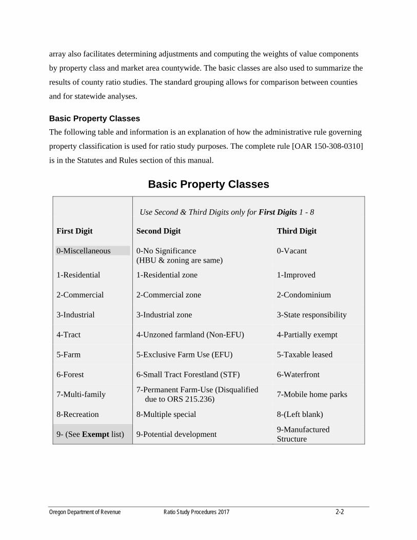
The following table and information is an explanation of how the administrative rule governing
property classification is used for ratio study purposes. The complete rule [OAR 150-308-0310]
is in the Statutes and Rules section of this manual.
Basic Property Classes
Use Second & Third Digits only for First Digits 1 - 8
First Digit
Second Digit
Third Digit
0-Miscellaneous
0-No Significance (HBU & zoning are same)
0-Vacant
1-Residential 1-Residential zone 1-Improved
2-Commercial 2-Commercial zone 2-Condominium
3-Industrial 3-Industrial zone 3-State responsibility
4-Tract 4-Unzoned farmland (Non-EFU) 4-Partially exempt
5-Farm 5-Exclusive Farm Use (EFU) 5-Taxable leased
6-Forest 6-Small Tract Forestland (STF) 6-Waterfront
7-Multi-family 7-Permanent Farm-Use (Disqualified
due to ORS 215.236) 7-Mobile home parks
8-Recreation 8-Multiple special 8-(Left blank)
9- (See Exempt list) 9-Potential development 9-Manufactured Structure
Oregon Department of Revenue Ratio Study Procedures 2017 2-3
1-0-0 Residential land only is an unimproved property that has residential use as its highest and best use (HBU), and the primary zoning is residential.
1-0-1 Residential property is an improved property that has residential use as its HBU. (The 0 indicates the HBU conforms to zoning.)
2-0-0 Commercial land only is an unimproved property that has commercial use as its HBU, and the primary zoning is commercial.
2-0-1 Commercial property is an improved property that has commercial use as its HBU. This HBU is as income-producing property. Examples of commercial property include, but are not limited to: retail stores, supermarkets, discount stores, department stores, convenience marts, financial institutions, office buildings, small retail laundries, dry cleaners, medical and dental office buildings, recreational vehicle parks, restaurants, theaters, automobile service stations and truck stops, automotive service centers, parking garages, car dealerships, hotels, and motels.
3-0-0 Industrial land only is an unimproved property that has industrial use as its HBU, and the primary zoning is industrial.
3-0-1 Industrial property is an improved property that has industrial use as its HBU. Industrial property includes, but is not limited to, those properties described by ORS 306.126, OAR 150-306-0090(1), and ORS 308.408. Industrial property is typically located in an industrial zone, but may be located in areas with other types of zoning, for example, if it is a pre-existing or conditional use. Property-use characteristics typically include assembly, processing or manufacturing products from raw materials or fabricated parts and include factories that render service, for example, large non-retail laundries, and dry cleaners. Examples of industrial property include, but are not limited to, steel plants, foundries, chemical plants, and assembly plants; saw mills, plywood plants, and wood pulp or paper mills; high technology facilities, research and development facilities, science parks, and light and heavy manufacturing facilities; storage and distribution warehouses (including mini-storage); natural resource processing and refining facilities such as natural gas wells and rock quarries. Classification of property as industrial is a separate determination from appraisal responsibility. Department or county responsibility for appraising industrial property is described in OAR 150-306-0090(1).
4-0-0 Tract land only is parcels of varying sizes of unimproved acreage where the HBU is for development to a suburban or rural homesite, but the land is not divided into urban-type lots.
4-0-1 Tract property is parcels of varying sizes of improved acreage where the HBU is for use as a suburban or rural homesite, but the land is not divided into urban-type lots.
5-0-0 Farm and range land is vacant land where the HBU is for the production of agricultural crops, feeding or management of livestock, or any other agricultural use. And, the land is not specially assessed for farm use.
Oregon Department of Revenue Ratio Study Procedures 2017 2-4
5-0-1 Farm and range property is land improved with buildings where the HBU is for the production of agricultural crops, feeding or management of livestock, or any other agricultural use. And, the land is not specially assessed for farm use.
5-4-0 Non-EFU zone farm and range land is vacant land that is under special farm use assessment by application.
5-4-1 Non-EFU zone farm and range property is land improved with buildings that is under special farm use assessment by application.
5-5-0 EFU zoned farm and range land is vacant land which is under special farm use assessment by zoning.
5-5-1 EFU zoned farm and range property is land improved with buildings which is under special farm use assessment by zoning.
6-0-0 Forest land is vacant land which has a HBU use for growing and harvesting trees of a marketable species.
6-0-1 Forest property is land improved with buildings which has a HBU for growing and harvesting trees of a marketable species.
6-4-0 Forest land is vacant land for which the HBU is other than growing and harvesting of trees of a marketable species and which has been designated as forest land by application.
6-4-1 Forest property is improved with buildings for which the HBU is other than growing and harvesting of trees of a marketable species and which has been designated as forest land by application.
6-6-0 Small Tract Forestland property is vacant land that is under special forestland assessment as Small Tract Forestland (STF) by application. 6-6-1 Small Tract Forestland property is land improved with buildings that is under special forestland assessment as STF by application.
7-0-0 Multi-family land is unimproved land that has multiple housing (five or more living units) as the HBU, and the primary zoning is multi-family.
7-0-1 Multi-family property is an improved property that has multiple housing (five or more living units) as its HBU, Multi-family property includes property developed as a manufacture housing park.
8-0-0 Recreation land is unimproved land that has recreational use as its HBU.
8-0-1 Recreation property is an improved property that provides recreational opportunity as its highest and best use.
Oregon Department of Revenue Ratio Study Procedures 2017 2-5
The property classification associated with the property may or may not be the current use
per OAR 150-308-0310(7)(a).
Mixed-use or transitional properties typically cannot be defined with the basic property
classifications listed above, but may be coded utilizing the Basic Property Classes table. Per
OAR 150-308-0310, the property class for mixed-use or transitional properties will be assigned
based upon the use that contributes the most to the real market value as of the current assessment
date. The property classification system must not be used to categorize market data that is more
accurately described by other characteristics, such as the quality class of the improvements,
market areas, or neighborhoods. Each digit of the code defines property as described in the
following explanations.
First Digit
The first digit of the property class code (as shown in column one of the Basic Property Classes
table) indicates the highest and best use (HBU) of property, except for specially assessed
property. It usually is the present use and typically reflects the current zoning. However, the first
digit code for non-conforming, mixed-use, or transitional property may be inconsistent with
zoning or the current use.
1 Residential: described as one to four family units 2 Commercial: uses include retail, office, financial institutions, offices etc. 3 Industrial: uses include assembly, manufacturing, or processing 4 Tract small: acreage parcels of at least one acre being used as suburban or rural
homesites 5 Farm: uses include rangeland or agricultural 6 Forest: activity includes growing and harvesting marketable timber 7 Multi-family: described as residential use of five or more living units 8 Recreation: used for recreational purposes
Second Digit
The second digit further categorizes the property. This number reflects the zoning or designates
the land as specially assessed. A zero indicates the HBU conforms to zoning. A second digit of 1,
2, or 3 indicates the designated zoning when the zoning is not the same as HBU of the property.
Use the following guide:
Oregon Department of Revenue Ratio Study Procedures 2017 2-6
0 No Significance: Indicates HBU of the property and zoning are the same. 1, 2, 3 Indicates HBU and zoning are not the same. Example: For a property located in a
commercial zone with a residential improvement and a residential HBU, the property class would be 1-2-1. If the HBU is commercial, the property class would be 201 regardless of the actual use.
4, 5 Indicates special assessment for farm-use and forest-use lands. 6 Indicates special assessment for Small Tract Forestland (STF). 7 Indicates property permanently disqualified from farm or forest land use due to
ORS 215.236 (nonfarm dwelling in exclusive farm use zone). 8 Indicates property carries more than one special assessment; i.e., combination of
farm use and designated forest land or other combination of special assessments. Also used for specially assessed, government-restricted multi-unit rental housing that is specially assessed under ORS 308.701 – ORS 308.724.
9 Indicates property has potential for further development, e.g., it has been subdivided or is sub-dividable.
Third Digit
The third digit is unique to the class and acts as an additional identifier.
0 Vacant: may have some onsite development (OSD) 1 Improved (typical of class) 2 Condominium 3 State responsibility: property appraised by the DOR 4 Partially exempt 5 Taxable leased: otherwise exempt property rented by a taxable owner 6 Waterfront 7 Mobile home park 8 (Left blank) 9 Manufactured structure
Miscellaneous Property: Class 0-x-x
Per OAR 150-308-0310(7)(b), unique properties can be classified under the miscellaneous
category. The miscellaneous category can also be used for property requiring a separate trend.
Properties classified as miscellaneous are assigned a number beginning with zero as described in
the Basic Property Classes table. When determining property class codes for miscellaneous
categories, apply the following coding system:
The first digit is always zero (0) and denotes the major class: Miscellaneous Property.

Oregon Department of Revenue Ratio Study Procedures 2017 2-7
The second digit indicates the basic class to which the property relates:
0-0-x Miscellaneous Property 0-1-x Miscellaneous Residential 0-2-x Miscellaneous Commercial 0-3-x Miscellaneous Industrial 0-4-x Miscellaneous Tract 0-5-x Miscellaneous Farm 0-6-x Miscellaneous Forest 0-7-x Miscellaneous Multi-family 0-8-x Miscellaneous Recreational 0-9-x Miscellaneous Exempt The third digit is unique to the class, further defining property characteristics:
0-x-0 Unbuildable size, Department of Environmental Quality, easement, right-of-way, etc.
0-x-1 Improvement only 0-x-2 Mineral interest 0-x-3 Centrally assessed (DOR responsibility: utilities, railroads, airlines) 0-x-4 Historic 0-x-5 Open space 0-x-6 (Left blank) 0-x-7 Timeshare property 0-x-8 Enterprise zone 0-x-9 Manufactured structure
Examples:
0-0-9 Real property manufactured structure 0-1-9 Personal property manufactured structure
Exempt Property: Class 9-x-x
Properties classified as exempt are assigned a property class number beginning with the digit
nine. When determining property class codes for exempt categories, apply the following coding
system:
The first digit is always nine (9) and defines the property as exempt. The second digit identifies the type of property or ownership:
9-0-x Student housing
Oregon Department of Revenue Ratio Study Procedures 2017 2-8
9-1-x Church 9-2-x School 9-3-x Cemetery 9-4-x City 9-5-x County 9-6-x State owned 9-7-x Federally owned 9-8-x Benevolent, fraternal ownership 9-9-x Port properties or other municipal properties The third digit is unique to this class and acts as an additional identifier:
9-x-0 Vacant 9-x-1 Improved 9-x-2 Partially exempt 9-x-3 Taxable leased property 9-x-4 In lieu of value (tax) 9-x-5 Temporarily exempt 9-x-6 Native American holdings 9-x-7 (Left blank) 9-x-8 Mineral interest 9-x-9 Manufactured structure
Examples:
9-0-1 OSU student housing 9-1-2 Church property with for-profit bookstore
Multi-Account Sales
Only one property classification should be included in the sales record. If a sale includes more
than one parcel and they are different property classifications, the predominant classification
should be used.
Machinery and Equipment ORS 308.215(2) (Statute amended in 2012)
(2)For purposes of the classification of real property required under subsection (1)(a)(C) of this section, property listed in paragraph (a), (b) or (c) of this subsection must be classified, together with any other property listed in the respective paragraph, separately from all other property:
(a) Machinery and equipment.
Oregon Department of Revenue Ratio Study Procedures 2017 2-9
(b) Property appraised under ORS 306.126, other than machinery and equipment.
(c) Industrial property, other than property appraised under ORS 306.126, and commercial property.
As of the date of this publication, the Department of Revenue has not addressed the property
classification of real property machinery and equipment (M&E) in an administrative rule.
However, DOR surveyed the counties and found the most common property classifications used
to identify real property M&E are 0-3-3, 0-3-6, 0-3-8, and 3-0-8.

Oregon Department of Revenue Ratio Study Procedures 2017 3-1
SECTION 3
SALES DATA COLLECTION AND STANDARD DATA FORMAT
The annual ratio study begins with the collection of information on property sales throughout the
county. All available sales should be used for each property class. This will avoid distortion of
the results and provide an accurate reflection of the assessment program.
Sales Data Year
The sales collection year is from January 1 through December 31. Collection of sales data
must be organized, timely, and continuous. It is advisable to have each month’s sales
completed by the last working day of the following month. The sales analysis process can
be started prior to the first of the year. The collection and processing of sales through
December should be completed and compiled by February 15.
After the sales data have been gathered and arrayed, analysis and computation begin.
Analysis for the current year and sales collection for the coming year overlap. As
statistical analysis begins for the current year, sales collection for the coming year is
taking place.
The certified ratio study is to be finalized and delivered to the DOR by July 1. The
department will consider an extension for cause, to last no later than August 1, if a
request is filed in writing with the department prior to July 1.
Market Data Sources
Sales information is taken from recorded instruments such as deeds, mortgages, and contracts.
Other information from unrecorded sources, such as comments from realtors or appraisers, can
be used only when thorough verification has been conducted.
Written procedures should be developed that outline the timely movement of the sales
information from the clerk’s office through the assessor’s office and then to the data analyst.
This process is known as sales take-off. The data analyst needs to ensure that the sales collection,
Oregon Department of Revenue Ratio Study Procedures 2017 3-2
confirmation, and qualification process is current.
Data Sources:
Primary sources for real property transactions include recorded and unrecorded property
transfers such as deeds, contracts, and mortgages.
Oregon Building Codes Division (BCD) is responsible for maintaining ownership and
siting information for manufactured structures. Most transactions take place through the
BCD LOIS System at the county assessor’s office or mobile home dealerships, which will
be acting on behalf of the division.
Secondary sources include individual buyers and sellers, and the records of real estate
offices; multiple-listings services; title companies; government and private sector fee
appraisers; building contractors; financial institutions; and developers.
Secondary sources are very important when data is limited. They can provide information
regarding market activity. A banker may explain a policy regarding sales after foreclosure, i.e.,
whether a sale price is at market value or at liquidation value. Real estate brokers can verify
whether a listing is above or below what the market reflects. Listing prices can be utilized in the
ratio study for supporting data only when they are adjusted for the typical differences between
the asking prices and final sale consideration. The adjustments must be developed in a special
study.
Sales Database
Pertinent information is maintained in a sales database. This is an organized filing system with
related market information, such as prices and trends from actual sales, real estate publications,
and regional economic and employment information. This information is used by the data analyst
to understand market activity and can be used to develop supplemental studies related to the ratio
and adjustment program.

Oregon Department of Revenue Ratio Study Procedures 2017 3-3
Property Sale Identification
It is important to identify each transaction in the computer generated sales database system with
the appropriate Map and Tax Lot numbers. Other identification numbers that can be used, not to
replace Map and Tax Lot numbers are:
Account number
Reference number
Key number
Serial number
Multi-Account Sales
When more than one account is included in a sale, all accounts need to be identified within the
database, and the total RMV of the land and improvements from the current certified roll of all
accounts involved must be used. These types of sales should be handled with caution because
they are more complex than the typical transaction of properties within the sales array.
Standard Data Format ORS 306.125(1)
Submit assessment and taxation information in standard data exchange formats as required by
ORS 308.215, 308.217, 308.219, 309.310, and 311.105.
The sales record or sales database should contain all pertinent information regarding
transactions. The sales listings and related statistical data will be developed from this
information. Not all information maintained in the sales record is used to create the sales listings.
The program should have the flexibility to sort on any of the data fields.
Provide the sales database, including all rejected sales, to the Department of Revenue, when
requested, under its supervisory responsibility and authority per ORS 306.115.
Database Fields
The following data fields should be included in any sales database. This database need not be
entirely separate from the assessment roll or other databases maintained by the county, provided
the analyst is able to store, view, and retrieve the necessary information.

Oregon Department of Revenue Ratio Study Procedures 2017 3-4
1. Grantor’s name — seller
2. Grantor’s address (optional)
3. Grantee’s name — buyer
4. Grantee’s address
5. Account number — consists of township, range, section, and tax lot numbers
6. Code area number — taxing district code
7. Instrument number — deed, volume and page numbers, instrument number, or other identifying numbers to locate the recordation of the deed or contract
8. City — city code numbers (if used)
9. Building class — the principal building class as shown on the appraisal inventory record, computer printout, or envelope. Other buildings shall be coded by type, enabling separate adjustments, if necessary.
10. Year built — the year the principal building was constructed
11. Percent good — a measure of depreciation (physical, functional, and economic) determined for the principal building.
12. Year appraised — the assessment year for which the field appraisal of the property was made. ORS 308.234.
This information allows separate studies of current RMV levels based on appraisals prepared in different years.
If the land and improvements were valued separately for different assessment years, the earliest date will be considered the year appraised.
For counties that recalculate, a revaluation is conducted on an annual basis. Care should be taken to maintain the actual year of last physical inspection of the property upon which the basic characteristics (square foot area, quality class, condition, other improvements, etc.) were determined as the year appraised.
13. Appraisal area — appraisal area within the county.
Counties are no longer required to maintain six appraisal maintenance areas.
Counties may continue to maintain six appraisal maintenance areas or identify new appraisal areas based on their needs analysis and available resources.
14. Market area — a group of properties that generally share important characteristics that influence value. See OAR 150-309-0230 and 150-308-0380.

Oregon Department of Revenue Ratio Study Procedures 2017 3-5
15. Acres (size) — total acres or square footage included in the transaction (if available).
16. Ratio — a percentage obtained by dividing the RMV from the current certified roll by the sale price (SP) (Roll RMV ÷ SP = Sales Ratio).
17. Condition (reject) code — a code showing the status of a sale that has either been disqualified or accepted for ratio study purposes. See Section 5 of this manual.
18. Condition code explanation — specific explanation as to why the condition code was selected.
19. Roll year — current assessment roll is the roll being prepared for the tax year beginning July 1 of the current calendar year, per OAR 150-309-0230(7).
Note: Prior year sales will have a different roll year than current year sales. These sales must be analyzed to determine if a trend exists and properly adjusted to the current assessment date.
20. Real market value — the RMV of land and improvements including manufactured structures taken from the current certified roll. RMV must reflect the condition of the property at the time of sale and not be influenced by consolidations, segregations, demolished, repairs, remodeling, or additions that were not included in the sale.
21. Sale price — the sale price or amount of consideration shown on the deed or contract.
22. Sale price data — (gathered from confirmation).
Terms: type of financing, down payment, interest rate, and duration of the mortgage
Conditions surrounding the sale (foreclosure, distress, open market, illness, length of time on market, etc.)
Encumbrances or liens assumed by the purchaser
Adjustments to the sale price: may include, but are not limited to, personal property, points paid by the grantor, repair allowances, any portions not assessed for property tax purposes included in the selling price (timber, crops, orchards)
23. Date of sale — the date the sale instrument was signed or the sale price was agreed upon between seller and buyer. The recordation date indicates the date the transaction became public record.
24. Property class — outlined in Section 3 or as specified in OAR 150-308-0310.
25. County number (1 - 36) — usable for multi-county ratio study report (see Addenda).
26. Instrument type — warranty deed, trust deed, contract, etc.

Oregon Department of Revenue Ratio Study Procedures 2017 3-6
27. Zoning — residential, commercial, industrial, EFU, etc.
28. Multiple-account indicator — more than one parcel (account) in transaction.
29. Comments.
30. Staff, including the data analyst, confirming sales.
31. Optional information — additional information may be captured, if determined appropriate. This may include items such as:
Storing an adjustment to a recorded price (for personal property)
Noting sales questionnaires have been sent or received
Storing the adjusted sale price and date
Identifying unusual properties (waterfront, etc.)
At this point, all sales have been organized but not analyzed.
Oregon Department of Revenue Ratio Study Procedures 2017 4-1
SECTION 4
INVESTIGATING SALE TRANSACTIONS
Sales Confirmation and Verification
Real estate sales provide the basis for valuing real property. Sales are also used to measure
equality and uniformity of assessment. The use of sales for these purposes has been tested in the
courts.
As data is collected, deeds and contracts should be carefully examined to identify characteristics
of individual sales. There may be sufficient information on the recorded instrument to support
rejecting the sale for use in the current ratio study. If not immediately rejected, an attempt should
be made to confirm the sale by mail or personal contact. Both confirmed and unconfirmed sales
are analyzed to create a listing of sales used to complete ratio studies.
The data analyst, registered appraisers, or other trained non-appraisal staff may complete
confirmation duties. The person confirming the sale should be identified in the sales file as well
as notation of the method used. Support staff may complete certain portions of the confirmation
process such as mailing sales questionnaires, recording responses, and data entry. It is important
to document when questionnaires were mailed or other forms of contact were attempted.
The assessor is responsible for developing written sales confirmation and verification procedures
to ensure consistency and uniformity in collection and screening of sales data. The terms
confirmation and verification are different in their definition:
Confirm is to cause someone to believe something more strongly.
Example: While obtaining information by telephone about a property sale, the buyer
states the information about the sale and inventory in the record is correct. This sale has
been confirmed.
Verify is to prove, show, or find out that something is true or correct; having first-hand
knowledge. It is a higher level of validation.
Example: Upon a field inspection, the appraiser interviewed the buyer and observed first-
Oregon Department of Revenue Ratio Study Procedures 2017 4-2
hand the information in the inventory record was correct. This sale has been verified.
Methods of Confirmation and Verification
All methods should follow a standardized format to maintain consistency of data collection. The
following is a list of commonly used methods and their level of affirmation. Each method is
described in more detail below.
Typical methods are:
Questionnaire letter - confirmation
Telephone - confirmation
Email or Internet digital form - confirmation
Field inspection and interview (Level 1, 2, or 3 inspection) - verification
Questionnaire Letter
The questionnaire letter is the most widely used method of sale confirmation and should be
customized for different property types. Letters should be on county letterhead and include the
purpose of the questionnaire along with county contact information. Some counties include a
postage-paid return envelope. See questionnaire examples at the end of this section.
Here are some considerations when evaluating responses:
Interest transferred (fee simple, partial, etc.)
Was this an arm’s length transaction?
o Was there a relationship between the buyer and seller?
o When was the price negotiated?
o How long was the property exposed to the market?
o Was either party under duress?
The stated reason for purchase.
When personal property is listed in the sale, determine how it affects the sale price.
Oregon Department of Revenue Ratio Study Procedures 2017 4-3
Did the sale price include unpaid taxes or assessments?
Were the closing costs/points paid by the seller?
Has the property changed since the sale price was negotiated?
If responses from both the buyer and seller are received, they should be carefully compared.
Did the buyer and seller provide the same sale date?
Did the buyer and the seller confirm the sale price and related terms?
Telephone Contact
Telephone confirmation is an effective method of confirming sales with the grantor, grantee, or
an agent directly involved in the transaction.
The caller should organize the interview prior to the call to make certain all necessary questions
are answered in one contact. Use the questionnaire as a guide to ensure the information gathered
is consistent.
Email or Internet Digital Form
Some counties have electronic questionnaires available on their website where interested parties
can provide sale confirmation.
Field Inspection
Field inspection and in-person interview provide the most confident level of affirmation of the
property characteristics and condition of sale for all properties (residential including
manufactured structures, farm, commercial, industrial, etc.). Complex property transactions such
as commercial, industrial, and farm properties, typically require an on-site field inspection. Such
sales usually involve both real and personal property.
The letter questionnaire can provide guidance to ensure that the information gathered is
consistent. Additional questions should be added that are specific to the type of property.
Levels 1, 2, and 3 are acceptable levels of inspection for field verification of sales (Appraisal
Methods Manual):
Oregon Department of Revenue Ratio Study Procedures 2017 4-4
Level 1. A full inspection, exterior and interior.
Level 2. An exterior inspection is made. No attempt at an interior inspection is made unless a major change to the property is detected.
Level 3. A street inspection is conducted. (Drive-by inspection only, unless a major change to the property is detected.)
Level 4. No on-site inspection is made. This level is intended for recalculation purposes only and is not valid for appraisal because property characteristics are not verified. Oblique aerial photography is in this category.
An Exception to Typical Confirmation Practices
Under certain circumstances, a choice not to confirm sales may be acceptable. This exception to
typical confirmation practices is to use only the consideration (sale price) directly from the
recording instrument. This exception should only be used for residential properties when:
There is a large quantity of sales
Sales can be documented as representative of properties in a study area
Confidence intervals are sufficiently narrow (+/- 5%)
Sample size can minimize the effect of extreme ratios on central tendencies. When using this
exception, all relevant sales in that market area must remain in the study (that are not found to
be unusable for ratio study purposes as in DOR Condition Codes 1-23). Do not eliminate sales
without sufficient and compelling information.
SALE ADJUSTMENTS AND QUALIFICATION
Adjustments to Identify and Consider
Property sales often include more than land and buildings and may contain certain obligations of
the buyer or seller. When sale prices include furniture, machinery, livestock, timber, orchard
trees, or farm crops, identify the item and the value allocated to each adjustment. Non-taxable
elements such as farm machinery and intangible business value should be subtracted from the
sale price. If a buyer assumes sewer or street assessments, delinquent property taxes, or other
title clearing ownership expenses, the sale price may need to be adjusted.
When evaluating these adjustments, consider the following:

Oregon Department of Revenue Ratio Study Procedures 2017 4-5
Does the amount adjusted appear reasonable?
What was the source of the value estimate?
What is the source of any revised value?
Multi-Account Sales
If a sale includes more than one parcel or account, care should be exercised that all accounts
have been included.
General Acceptance of Sales
In evaluating each sale, it is critical to determine whether the sale meets the standards for
inclusion in the ratio study. If a sale cannot be confirmed and there is no apparent reason to reject
it, the sale must be included in the ratio study. Attempts to confirm these sales should be
documented in the sale listing.
The sales reviewer should take the position that all sales are candidates as valid sales for the ratio study unless sufficient and compelling information can be documented to show otherwise. If sales are excluded without substantiation, the study may appear to be subjective. Reason codes can be established for invalid sales. (IAAO Standard on Ratio Studies, 2013, page 48)
Identifying Unusable Sales
The following types of sales are generally found to be unusable for ratio study purposes.
Conditions that may invalidate a sale include but are not limited to:
1. Sales involving government agencies, public utilities, and educational institutions. Such sales can involve an element of compulsion (eminent domain) and often occur at prices higher than would otherwise be expected in the market. Liquidation sales may reflect a lower than typical market price.
2. Sales involving charitable or religious organizations. A sale involving these
organizations can include an element of philanthropy and may contain an atypical consideration or restrictive covenant.
3. Sales involving financial institutions. A sale in which the lienholder is the buyer may be in lieu of a foreclosure or a judgment and the sale price can equal the loan balance only.
4. Sales between relatives or corporate affiliates. These sales are usually not open market, arm’s length transactions.
Oregon Department of Revenue Ratio Study Procedures 2017 4-6
5. Sales settling an estate. A conveyance by an executor or trustee under powers granted in a will may not represent fair market value. Verify if the sale took place soon after the will was filed and admitted to probate in order to satisfy debts or the wishes of an heir.
6. Forced sales. Such sales include those resulting from a judicial order. The seller in such cases is usually a sheriff, receiver, or other court officer.
7. Sales of doubtful title. When a sale is made on other than a warranty deed, there is a question of whether the title is merchantable. Quit claim deeds and trustees’ deeds are examples.
8. Property description: Incorrect legal description. Deed may describe a parcel with ownership other than grantor or legal description may not be complete.
9. Partial interest and segregation: Partial interest sales and segregations may not represent true real market value of the entire property on the roll.
10. Acquisitions or Divestments by Real Estate Investors: Purchases or sales by large corporations, pension funds, or real estate investment trusts (REITs) that involve multiple parcels.
Sales with Special Conditions
Sales with special conditions may be open-market transactions, and with thorough and complete verification, may qualify for use in ratio studies. 1. Land contracts: Current contract sales exposed to the market in the normal manner and
having terms similar to typical open-market transactions (down payment, interest rates, and duration of loan) may qualify for use in the ratio study. Deeds in fulfillment of a land contract often reflect market conditions several years in the past, and such dated information should not be included in the ratio analysis.
2. Auctions: Auction sales of real property tend to be at the lower end of the price range. When verification reveals properties have been well-advertised and the auction well-attended, the sales may be valid for consideration in ratio studies.
3. IRS Revenue Code 1031 Exchanges: These are in almost all cases valid transactions
between knowledgeable parties who researched the available market and conducted this exchange to defer a capital gains tax event. One of the main criteria in this kind of exchange requires the party selling an investment property to reinvest in like kind of property for equal or greater value than the relinquished property. Acceptable exchanges under IRC 1031 include real property with real property, personal property with personal property, aircraft with aircraft, etc., of equal or greater value. This type of transaction is subject to a time-period limitation.
4. Property Sold Not Same as Appraised: If property sells in a condition that is different from
the way it had been valued, under certain circumstances it can be revalued and used in a ratio

Oregon Department of Revenue Ratio Study Procedures 2017 4-7
study. However, this is generally not the case. The caution in this instance is that property characteristics of the sold property are known while the current characteristics of the unsold properties in that study area remain unknown.
Prior to inclusion of the revalued sale in the ratio study, the following conditions must be met: There are no significant changes in the property rights transferred or in the permitted use,
and the parcel was not divided since the last appraisal date The sale is representative of the study area (see IAAO Section 4.5 on “Sample
Representativeness” below) The properties in the study area were appraised within the most recent five years using
the same date of value and appraisal procedure (see IAAO Section 4.8 on “Frequency of Reappraisals” below)
The sold property is revalued to reflect current characteristics of the sold property utilizing the same setup studies as the unsold properties in that study area
Excerpt from IAAO Standard on Ratio Studies, 2013:
Section 4.5, “Sample Representativeness:” In general, a ratio study is valid to the extent that the sample is sufficiently representative of the population. The distribution of ratios in the population cannot be ascertained directly and appraisal accuracy can vary from property to property. By definition, a ratio study sample would be representative when the distribution of ratios of properties in the sample reflects the distribution of ratios of properties in the population. Representativeness is improved when the sample proportionately reflects major property characteristics present in the population of sold and unsold properties. As long as sold and unsold parcels are appraised in the same manner and the sample is otherwise representative, statistics calculated in a sales ratio study can be used to infer appraisal performance for unsold parcels.
However, if parcels that sell are selectively reappraised based on their sale prices and if such parcels are in the ratio study, uniformity inferences will not be accurate (appraisals appear more uniform than they are). In this situation, measures of appraisal level also will not be supportable unless similar unsold parcels are appraised by a model that produces the same overall percentage of market value (appraisal level) as on the parcels that sold (see Appendix E, ”Sales Chasing Detection Techniques”). Assessing officials must incorporate a quality control program; including checks and audits of the data, to ensure that sold and unsold parcels are appraised at the same level.
Excerpt from IAAO Standard on Mass Appraisal of Real Property, 2013:
Section 4.8, “Frequency of Reappraisals:” Section 4.2.2 of the Standard on Property Tax Policy (IAAO 2010) states that current market value implies annual assessment of all property. Annual assessment does not necessarily mean, however, that each property must be re-examined each year. Instead,
Oregon Department of Revenue Ratio Study Procedures 2017 4-8
models can be recalibrated or market adjustment factors derived from ratio studies or other market analyses applied based on criteria such as property type, location, size, and age. Analysis of ratio study data can suggest groups or strata of properties in greatest need of physical review. In general, market adjustments can be highly effective in maintaining equity when appraisals are uniform within strata and recalibration can provide even greater accuracy. However, only physical reviews can correct data errors and, as stated in Sections 3.3.4 and 3.3.5, property characteristics data should be reviewed and updated at least every 4 to 6 years. This can be accomplished in at least three ways: • Re-inspecting all property at periodic intervals (i.e., every 4 to 6 years) • Re-inspecting properties on a cyclical basis (e.g., one-fourth or one-sixth each year) • Re-inspecting properties on a priority basis as indicated by ratio studies or other considerations while still ensuring that all properties are examined at least every sixth year
Sales or transaction instruments deemed unusable for the ratio study purposes may have valid
uses in other studies, such as appraisal setup, etc. When used in other studies, make proper
adjustments for date of sale and any subsequent changes to the property since the last appraisal
or valuation.
Condition Codes (IAAO Reason Code)
Once confirmation and verification is complete, a final condition code is applied. Condition
codes were developed to provide a numeric means of categorizing property sales by the
circumstances surrounding the transaction. The code represents the most compelling sale
condition description, which ties to its usability in the ratio study. This list can be expanded to fit
the individual needs of a county. The county’s complete condition code list must be included in
the ratio study report.
It is critical to select and assign the most appropriate condition code and then record it in the sale
condition data field. Sales can be sorted by the condition code for use in the ratio study.
Oregon Department of Revenue Ratio Study Procedures 2017 4-9
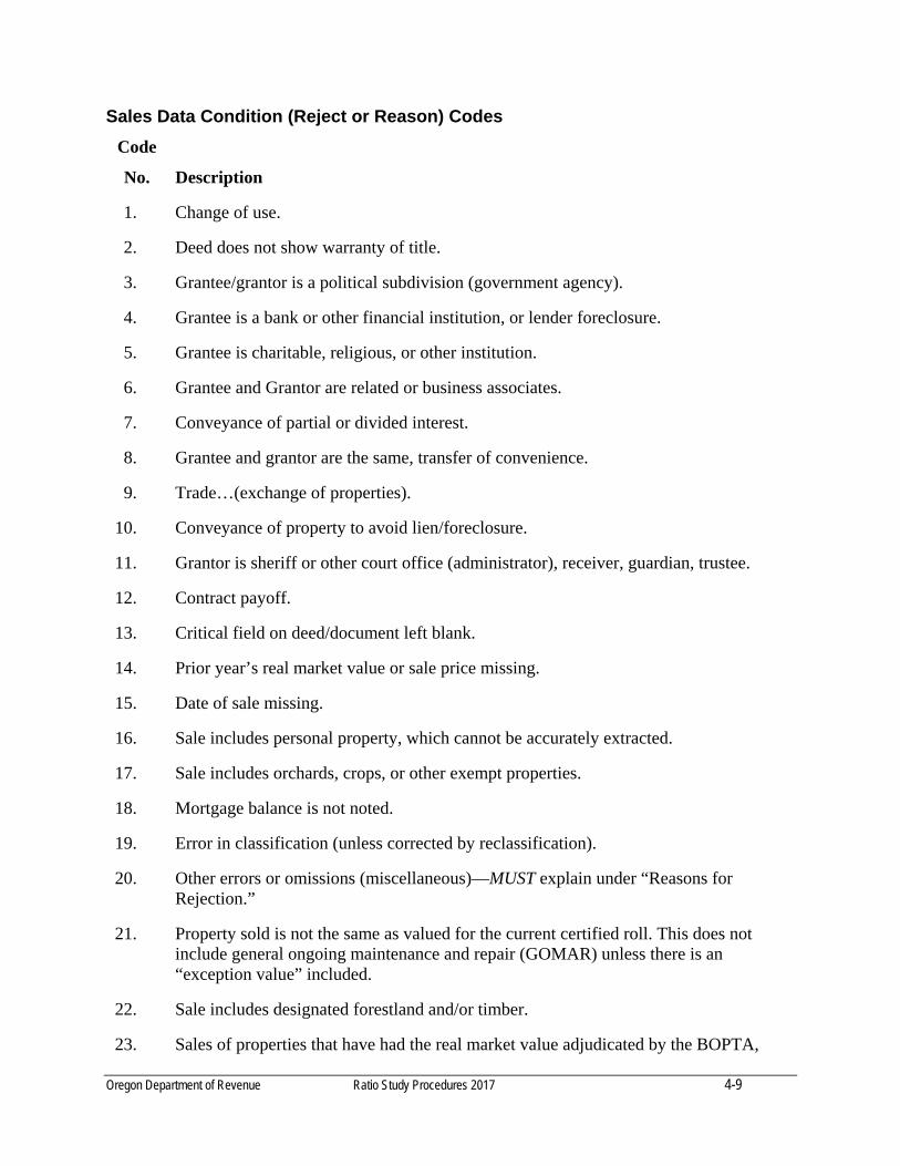
Sales Data Condition (Reject or Reason) Codes
Code
No. Description
1. Change of use.
2. Deed does not show warranty of title.
3. Grantee/grantor is a political subdivision (government agency).
4. Grantee is a bank or other financial institution, or lender foreclosure.
5. Grantee is charitable, religious, or other institution.
6. Grantee and Grantor are related or business associates.
7. Conveyance of partial or divided interest.
8. Grantee and grantor are the same, transfer of convenience.
9. Trade…(exchange of properties).
10. Conveyance of property to avoid lien/foreclosure.
11. Grantor is sheriff or other court office (administrator), receiver, guardian, trustee.
12. Contract payoff.
13. Critical field on deed/document left blank.
14. Prior year’s real market value or sale price missing.
15. Date of sale missing.
16. Sale includes personal property, which cannot be accurately extracted.
17. Sale includes orchards, crops, or other exempt properties.
18. Mortgage balance is not noted.
19. Error in classification (unless corrected by reclassification).
20. Other errors or omissions (miscellaneous)—MUST explain under “Reasons for Rejection.”
21. Property sold is not the same as valued for the current certified roll. This does not include general ongoing maintenance and repair (GOMAR) unless there is an “exception value” included.
22. Sale includes designated forestland and/or timber.
23. Sales of properties that have had the real market value adjudicated by the BOPTA,
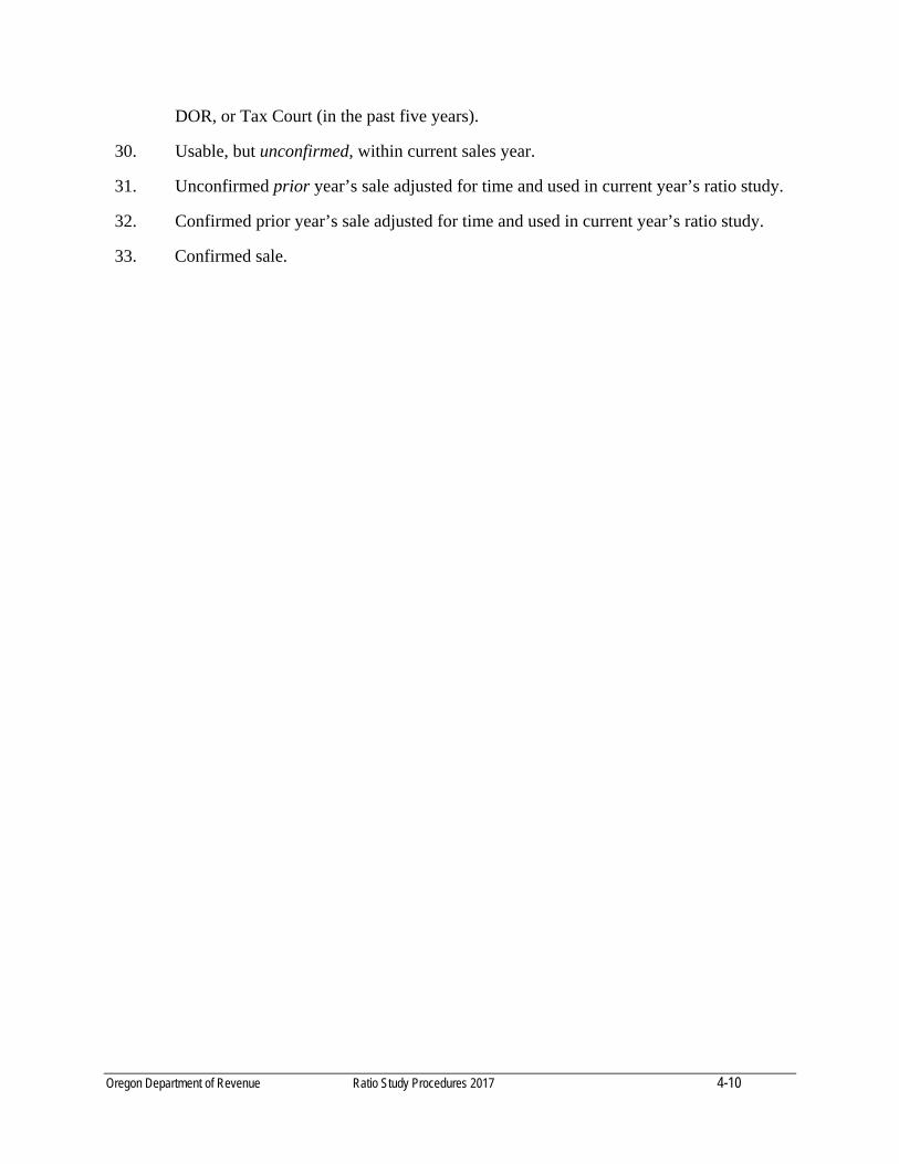
Oregon Department of Revenue Ratio Study Procedures 2017 4-10
DOR, or Tax Court (in the past five years).
30. Usable, but unconfirmed, within current sales year.
31. Unconfirmed prior year’s sale adjusted for time and used in current year’s ratio study.
32. Confirmed prior year’s sale adjusted for time and used in current year’s ratio study.
33. Confirmed sale.
Oregon Department of Revenue Ratio Study Procedures 2017 4-11
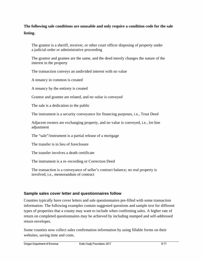
The following sale conditions are unusable and only require a condition code for the sale
listing.
The grantor is a sheriff, receiver, or other court officer disposing of property under a judicial order or administrative proceeding
The grantor and grantee are the same, and the deed merely changes the nature of the interest in the property
The transaction conveys an undivided interest with no value
A tenancy in common is created
A tenancy by the entirety is created
Grantor and grantee are related, and no value is conveyed
The sale is a dedication to the public
The instrument is a security conveyance for financing purposes, i.e., Trust Deed
Adjacent owners are exchanging property, and no value is conveyed, i.e., lot-line adjustment
The “sale”/instrument is a partial release of a mortgage
The transfer is in lieu of foreclosure
The transfer involves a death certificate
The instrument is a re–recording or Correction Deed
The transaction is a conveyance of seller’s contract balance; no real property is involved, i.e., memorandum of contract
Sample sales cover letter and questionnaires follow
Counties typically have cover letters and sale questionnaires pre-filled with some transaction information. The following examples contain suggested questions and sample text for different types of properties that a county may want to include when confirming sales. A higher rate of return on completed questionnaires may be achieved by including stamped and self-addressed return envelopes.
Some counties now collect sales confirmation information by using fillable forms on their websites, saving time and costs.

Oregon Department of Revenue Ratio Study Procedures 2017 4-12
Sample Cover Letter
Dear Property Owner:
Each year, we are required by law (ORS 309.200) to conduct sales studies using information
acquired from recorded documents (deeds, contracts, etc.). Please take a few moments to
complete the questionnaire.
Why is the sales information needed?
It is important for the assessor’s office to confirm the details of this property sale in order to
maintain uniform and equitable assessment. Sales of real estate are used as the main basis in
establishing the market value of land, buildings, and other improvements.
How will the information be used?
Appraisers will consider the selling price and other details from the questionnaire, along with the
selling prices of similar properties, to determine the market value for many properties.
Information about current building construction costs, income and expenses (for income
producing properties), condition of the buildings, etc., will be used in various valuation studies.
Why are so many questions asked about my property?
The deed provides the recorded sale price of the property, but does not include all necessary
information to complete a proper evaluation of the sale. Sales prices may include special
conditions, furniture, machinery, timber, livestock, and farm crops. The value of these items is
considered separately from the total selling price when the sales are analyzed.
What other details should be noted?
Crops, timber, plants, and orchard trees are not taxable. If the purchase price included any of
these items, please show the number of acres and type of item. Some property included in the
sale may not be assessable for property tax purposes. Amounts paid to the seller for sewer or
street assessments, property taxes, or other expenses should be listed. Since this information is
typically not provided on the deed, it is essential to notify the assessor about these special
County Letterhead Here
Oregon Department of Revenue Ratio Study Procedures 2017 4-13
conditions of the sale.
Oregon Department of Revenue Ratio Study Procedures 2015 4-14
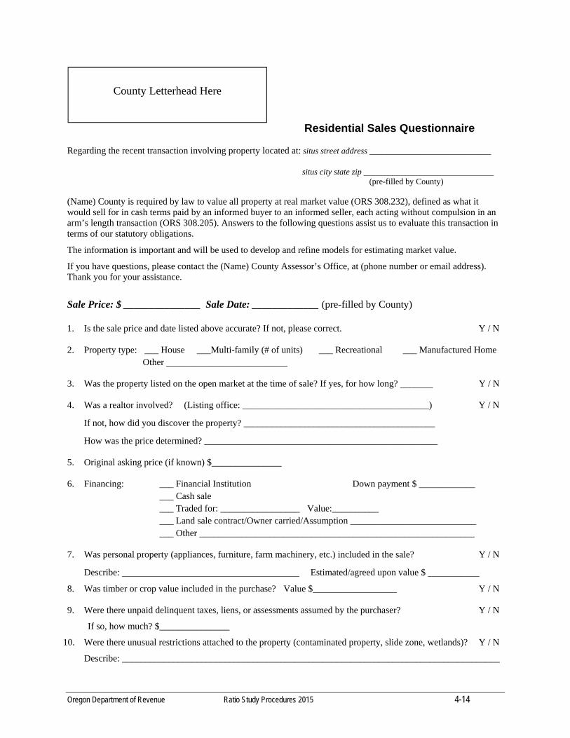
Residential Sales Questionnaire Regarding the recent transaction involving property located at: situs street address _____________________________
situs city state zip _______________________________ (pre-filled by County) (Name) County is required by law to value all property at real market value (ORS 308.232), defined as what it would sell for in cash terms paid by an informed buyer to an informed seller, each acting without compulsion in an arm’s length transaction (ORS 308.205). Answers to the following questions assist us to evaluate this transaction in terms of our statutory obligations.
The information is important and will be used to develop and refine models for estimating market value.
If you have questions, please contact the (Name) County Assessor’s Office, at (phone number or email address). Thank you for your assistance.
Sale Price: $ _______________ Sale Date: _____________ (pre-filled by County) 1. Is the sale price and date listed above accurate? If not, please correct. Y / N
2. Property type: ___ House ___Multi-family (# of units) ___ Recreational ___ Manufactured Home Other __________________________
3. Was the property listed on the open market at the time of sale? If yes, for how long? _______ Y / N 4. Was a realtor involved? (Listing office: ________________________________________) Y / N
If not, how did you discover the property? _________________________________________
How was the price determined? __________________________________________________
5. Original asking price (if known) $_______________
6. Financing: ___ Financial Institution Down payment $ ____________ ___ Cash sale ___ Traded for: _________________ Value:__________ ___ Land sale contract/Owner carried/Assumption ___________________________ ___ Other ___________________________________________________________
7. Was personal property (appliances, furniture, farm machinery, etc.) included in the sale? Y / N
Describe: ______________________________________ Estimated/agreed upon value $ ___________
8. Was timber or crop value included in the purchase? Value $__________________ Y / N
9. Were there unpaid delinquent taxes, liens, or assessments assumed by the purchaser? Y / N
If so, how much? $_______________
10. Were there unusual restrictions attached to the property (contaminated property, slide zone, wetlands)? Y / N
Describe: _________________________________________________________________________________
County Letterhead Here
Oregon Department of Revenue Ratio Study Procedures 2015 4-15
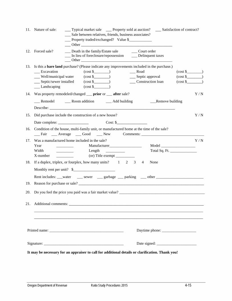
11. Nature of sale: ___ Typical market sale ___ Property sold at auction? ___ Satisfaction of contract? ___ Sale between relatives, friends, business associates? ___ Property traded/exchanged? Value $____________ ___ Other ________________________________________________
12. Forced sale? ___ Death in the family/Estate sale ___ Court order ___ In lieu of foreclosure/repossession ___ Delinquent taxes ___ Other ________________________________________________
13. Is this a bare land purchase? (Please indicate any improvements included in the purchase.) ___ Excavation (cost $________) ___ Road (cost $________) ___ Well/municipal water (cost $________) ___ Septic approval (cost $________) ___ Septic/sewer installed (cost $________) ___ Construction loan (cost $________) ___ Landscaping (cost $________)
14. Was property remodeled/changed ___ prior or ___ after sale? Y / N
___ Remodel ___ Room addition ___ Add building ___Remove building
Describe: __________________________________________________________________
15. Did purchase include the construction of a new house? Y / N
Date complete: ________________ Cost: $________________
16. Condition of the house, multi-family unit, or manufactured home at the time of the sale? ___ Fair ___ Average ___ Good ___ New Comments: _________________________________
17. Was a manufactured home included in the sale? Y / N Year _________ Manufacturer_________________ Model __________________ Width _________ Length __________ Total Sq. Ft. ______________ X-number _________ (or) Title exempt __________
18. If a duplex, triplex, or fourplex, how many units? 1 2 3 4 None
Monthly rent per unit? $______________________
Rent includes: ___water ___ sewer ___ garbage ___ parking ___ other _________________________
19. Reason for purchase or sale? __________________________________________________________________
20. Do you feel the price you paid was a fair market value? _____________________________________________
21. Additional comments: _______________________________________________________________________
_________________________________________________________________________________________
_________________________________________________________________________________________
Printed name: _______________________________________ Daytime phone: __________________
Signature: __________________________________________ Date signed: _____________________
It may be necessary for an appraiser to call for additional details or clarification. Thank you!
Oregon Department of Revenue Ratio Study Procedures 2015 4-16
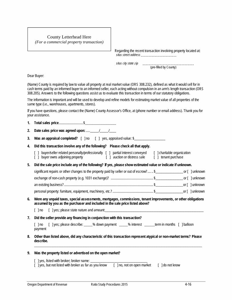
Regarding the recent transaction involving property located at:
situs street address _______________________
situs city state zip _________________________________ (pre-filled by County) Dear Buyer: (Name) County is required by law to value all property at real market value (ORS 308.232), defined as what it would sell for in cash terms paid by an informed buyer to an informed seller, each acting without compulsion in an arm’s length transaction (ORS 308.205). Answers to the following questions assist us to evaluate this transaction in terms of our statutory obligations.
The information is important and will be used to develop and refine models for estimating market value of all properties of the same type (i.e., warehouses, apartments, stores).
If you have questions, please contact the (Name) County Assessor’s Office, at (phone number or email address). Thank you for your assistance.
1. Total sales price ............................ $__________________
2. Date sales price was agreed upon: ..... _____/_____/____
3. Was an appraisal completed? [ ] no [ ] yes, appraised value: $__________________
4. Did this transaction involve any of the following? Please check all that apply.
[ ] buyer/seller related personally/professionally [ ] partial interest conveyed [ ] charitable organization [ ] buyer owns adjoining property [ ] auction or distress sale [ ] tenant purchase
5. Did the sale price include any of the following? If yes, please show estimated value or indicate if unknown.
significant repairs or other changes to the property paid by seller or out of escrow?.... .. $________________ or [ ] unknown
exchange of non-cash property (e.g. 1031 exchange)? ................................................. $________________ or [ ] unknown
an existing business? ....................................................................................................... $________________or [ ] unknown
personal property: furniture, equipment, machinery, etc.? ............................................... $________________or [ ] unknown
6. Were any unpaid taxes, special assessments, mortgages, commissions, tenant improvements, or other obligations assumed by you as the purchaser and included in the sale price listed above?
[ ] no [ ] yes; please state nature and amount:_________________________________________________________
7. Did the seller provide any financing in conjunction with this transaction?
[ ] no [ ] yes; please describe: _____% down payment _____% interest ______term in months [ ] balloon payment
8. Other than listed above, did any characteristic of this transaction represent atypical or non-market terms? Please describe. _________________________________________________________________________________________________
9. Was the property listed or advertised on the open market?
[ ] yes, listed with broker; broker name: _________________________________ [ ] yes, but not listed with broker as far as you know [ ] no, not on open market [ ] do not know
County Letterhead Here
(For a commercial property transaction)
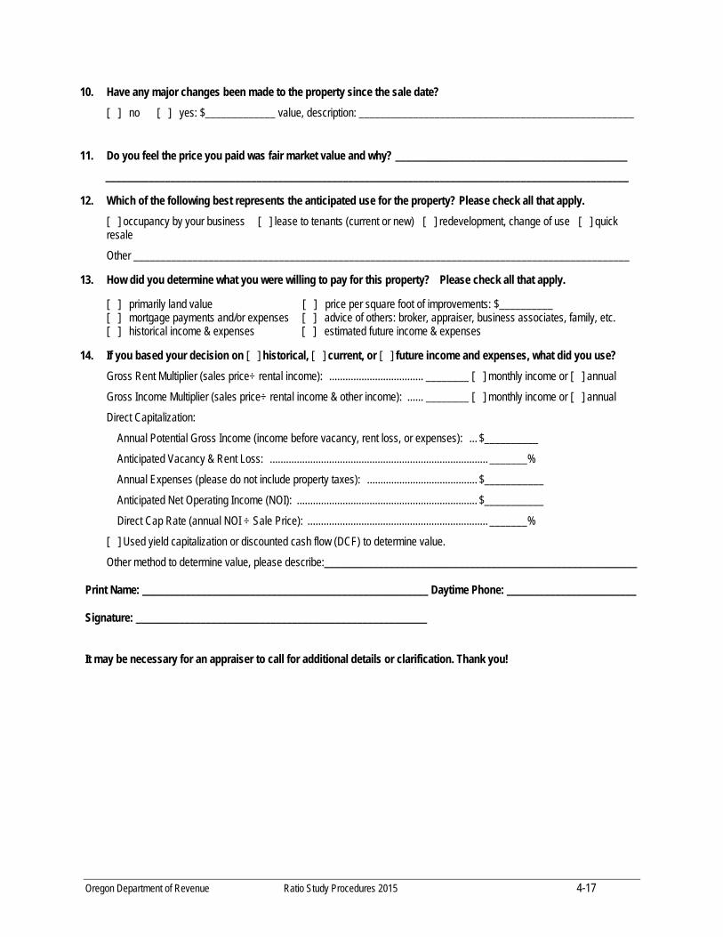
Oregon Department of Revenue Ratio Study Procedures 2015 4-17
10. Have any major changes been made to the property since the sale date?
[ ] no [ ] yes: $_____________ value, description: ___________________________________________________
11. Do you feel the price you paid was fair market value and why? ___________________________________________
_________________________________________________________________________________________________
12. Which of the following best represents the anticipated use for the property? Please check all that apply.
[ ] occupancy by your business [ ] lease to tenants (current or new) [ ] redevelopment, change of use [ ] quick resale
Other ____________________________________________________________________________________________
13. How did you determine what you were willing to pay for this property? Please check all that apply.
[ ] primarily land value [ ] price per square foot of improvements: $__________ [ ] mortgage payments and/or expenses [ ] advice of others: broker, appraiser, business associates, family, etc. [ ] historical income & expenses [ ] estimated future income & expenses
14. If you based your decision on [ ] historical, [ ] current, or [ ] future income and expenses, what did you use?
Gross Rent Multiplier (sales price÷ rental income): ................................... ________ [ ] monthly income or [ ] annual
Gross Income Multiplier (sales price÷ rental income & other income): ...... ________ [ ] monthly income or [ ] annual
Direct Capitalization:
Annual Potential Gross Income (income before vacancy, rent loss, or expenses): ... $__________
Anticipated Vacancy & Rent Loss: ................................................................................. _______%
Annual Expenses (please do not include property taxes): ......................................... $___________
Anticipated Net Operating Income (NOI): ................................................................... $___________
Direct Cap Rate (annual NOI ÷ Sale Price): ................................................................... _______%
[ ] Used yield capitalization or discounted cash flow (DCF) to determine value.
Other method to determine value, please describe:__________________________________________________________
Print Name: _____________________________________________________ Daytime Phone: ________________________
Signature: ______________________________________________________
It may be necessary for an appraiser to call for additional details or clarification. Thank you!
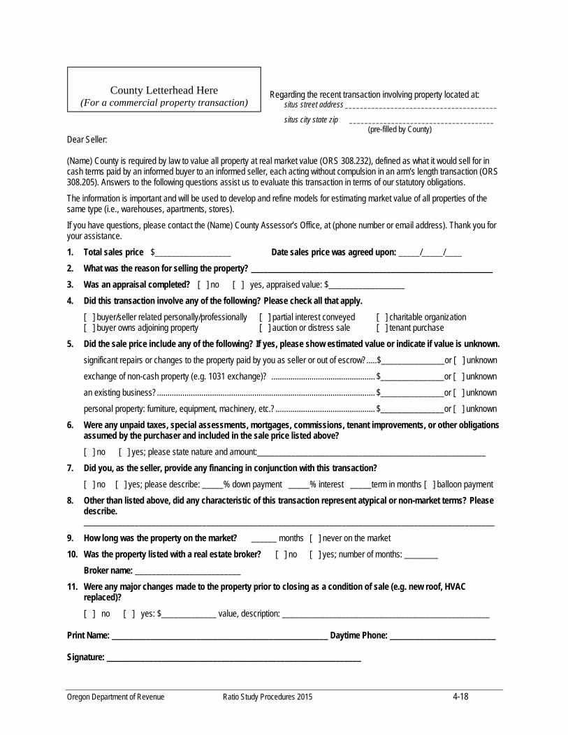
Oregon Department of Revenue Ratio Study Procedures 2015 4-18
Regarding the recent transaction involving property located at: situs street address ________________________________________
situs city state zip ______________________________________ (pre-filled by County) Dear Seller: (Name) County is required by law to value all property at real market value (ORS 308.232), defined as what it would sell for in cash terms paid by an informed buyer to an informed seller, each acting without compulsion in an arm’s length transaction (ORS 308.205). Answers to the following questions assist us to evaluate this transaction in terms of our statutory obligations.
The information is important and will be used to develop and refine models for estimating market value of all properties of the same type (i.e., warehouses, apartments, stores).
If you have questions, please contact the (Name) County Assessor’s Office, at (phone number or email address). Thank you for your assistance.
1. Total sales price $__________________ Date sales price was agreed upon: _____/_____/____
2. What was the reason for selling the property? _________________________________________________________
3. Was an appraisal completed? [ ] no [ ] yes, appraised value: $__________________
4. Did this transaction involve any of the following? Please check all that apply.
[ ] buyer/seller related personally/professionally [ ] partial interest conveyed [ ] charitable organization [ ] buyer owns adjoining property [ ] auction or distress sale [ ] tenant purchase
5. Did the sale price include any of the following? If yes, please show estimated value or indicate if value is unknown.
significant repairs or changes to the property paid by you as seller or out of escrow?.....$_______________or [ ] unknown
exchange of non-cash property (e.g. 1031 exchange)? ................................................. $_______________or [ ] unknown
an existing business? ....................................................................................................... $_______________or [ ] unknown
personal property: furniture, equipment, machinery, etc.? ............................................... $_______________or [ ] unknown
6. Were any unpaid taxes, special assessments, mortgages, commissions, tenant improvements, or other obligations assumed by the purchaser and included in the sale price listed above?
[ ] no [ ] yes; please state nature and amount:______________________________________________________
7. Did you, as the seller, provide any financing in conjunction with this transaction?
[ ] no [ ] yes; please describe: _____% down payment _____% interest _____term in months [ ] balloon payment
8. Other than listed above, did any characteristic of this transaction represent atypical or non-market terms? Please describe. _________________________________________________________________________________________________
9. How long was the property on the market? ______ months [ ] never on the market
10. Was the property listed with a real estate broker? [ ] no [ ] yes; number of months: ________
Broker name: _________________________
11. Were any major changes made to the property prior to closing as a condition of sale (e.g. new roof, HVAC replaced)?
[ ] no [ ] yes: $_____________ value, description: _________________________________________________
Print Name: ___________________________________________________ Daytime Phone: _________________________
Signature: ____________________________________________________________
County Letterhead Here
(For a commercial property transaction)
Oregon Department of Revenue Ratio Study Procedures 2015 4-19
It may be necessary for an appraiser to call for additional details or clarification. Thank you!

Oregon Department of Revenue Ratio Study Procedures 2017 5-1
SECTION 5
DATA ORGANIZATION:
RATIO CALCULATION, OUTLIERS, & TRIMMING
Ratio Calculation
The analyst accesses the sales listing database and selects all usable sales in a specific property
class or market area and arrays (an ordered list) them in a sales list including but not limited to
the following: condition code, property class, account number, land value, land size,
improvement value, total real market value, sale price, sale date, the sale ratio and other data
pertinent to the analysis.
Comparing the real market value (RMV) on the roll as of January 1 to the sale price (SP) results
in a relative relationship called a sales ratio (Ratio). The objective of the ratio is to measure the
validity of the roll values, meaning how the roll values compare to the sale prices.
RMV/SP = RATIO
Example: RMV on the roll is $99,830. Sale price is $125,000.
$99,830/$125,000 = 0.79864 rounded to 0.80 or 80% or 80
A sales ratio can be expressed as a percent or decimal. The common practice is to express the
ratio as a whole number.
The following, Exhibit SL-1, is an example of sales arrayed by ratios in ascending order.

Oregon Department of Revenue Ratio Study Procedures 2017 5-2
Sale # MA
Property
Class
Condition
Code Acct # Map & Taxlot
Instrument
Number Acres Land RMV Imp RMV Total RMV Sale Price Sale Date
Sale
Ratio
29 1 101 34 20115 18S4709 4110 3615 0.18 29,790 66,530 96,320 169,400 08/02/13 57
9 1 101 34 1216 18S4704DA 2900 4263 0.15 24,070 29,450 53,520 78,000 04/03/13 69
46 1 101 33 1427 18S4704DA 9200 2730 0.13 19,880 34,340 54,220 78,000 10/14/13 70
24 1 101 33 2161 18S4709AA 8500 2819 0.15 25,440 82,760 108,200 145,000 06/07/13 75
22 1 101 33 1443 18S4704DC 1400 2809 0.21 30,550 67,720 98,270 129,999 06/06/13 76
12 1 101 33 2815 18S4709CD 1800 4289 0.24 34,470 88,470 122,940 160,000 04/12/13 77
33 1 101 33 20240 18S4705AD 109 3485 0.29 43,770 96,030 139,800 175,000 09/07/13 80
42 1 101 33 1000 18S4704CC 3100 2839 0.22 31,460 68,370 99,830 125,000 10/08/13 80
13 1 101 33 1401 18S4704DB 6500 4795 0.26 38,480 59,240 97,720 120,000 04/12/13 81
19 1 101 34 980 18S4704CC 1900 2799 0.26 38,480 49,390 87,870 108,600 06/02/13 81
28 1 101 33 950 18S4704CC 100 1482 0.22 31,460 65,450 96,910 117,500 07/11/13 82
25 1 101 34 1446 18S4704DC 1700 4257 0.17 28,730 37,700 66,430 80,000 06/09/13 83
48 1 101 34 1601 18S4705AC 7500 4065 0.24 34,470 90,150 124,620 150,500 11/08/13 83
51 1 101 33 19844 18S4705AD 237 4196 0.24 34,470 115,220 149,690 179,000 12/01/13 84
23 1 101 33 1774 18S4705DA 4001 4866 0.24 34,470 58,910 93,380 109,900 06/06/13 85
36 1 101 33 15298 18S4705DD 4200 4551 0.16 27,360 72,440 99,800 117,500 09/10/13 85
34 1 101 33 1814 18S4705DA 8100 2579 0.25 37,110 71,400 108,510 126,000 09/09/13 86
11 1 101 33 1143 18S4704CD 7000 2963 0.22 31,460 112,020 143,480 165,000 04/06/13 87
32 1 101 34 918 18S4704CB 1106 3190 0.24 34,470 82,180 116,650 133,000 08/08/13 88
47 1 101 34 20235 18S4705AD 104 2555 0.24 34,470 117,920 152,390 174,000 11/02/13 88
15 1 101 34 20265 18S4705DA 602 4117 0.23 33,100 98,560 131,660 147,193 05/03/13 89
45 1 101 33 1710 18S4705C 7900 2670 0.22 31,460 93,410 124,870 139,900 10/13/13 89
7 1 101 34 18843 18S4704BC 3500 3818 0.23 33,100 55,980 89,080 99,500 03/11/13 90
20 1 101 33 19083 18S4705C 9200 4320 0.32 54,030 174,820 228,850 254,000 06/05/13 90
54 1 101 34 19110 18S4705C 11900 4059 0.32 54,030 200,990 255,020 280,000 12/15/13 91
14 1 101 34 19837 18S4705AD 230 1031 0.29 43,770 200,380 244,150 263,000 05/01/13 93
3 1 101 34 20196 18S4705DA 701 4556 0.26 38,480 103,740 142,220 149,963 02/04/13 95
37 1 101 34 1087 18S4704CD 1500 3547 0.17 28,730 54,590 83,320 88,000 09/14/13 95
38 1 101 34 19691 18S4705BD 1400 4633 0.29 43,770 146,850 190,620 197,000 09/15/13 97
17 1 101 34 15619 18S4705DB 9600 1478 0.31 51,530 158,610 210,140 214,000 05/10/13 98
31 1 101 33 8094 18S4705DB 1700 5027 0.30 50,620 67,600 118,220 120,000 08/06/13 99
30 1 101 33 2124 18S4709AA 5001 4017 0.13 19,880 17,690 37,570 37,500 08/04/13 100
43 1 101 33 19307 18S4704BC 7400 4513 0.23 33,100 78,860 111,960 112,000 10/11/13 100
50 1 101 34 786 18S4704BD 3900 1328 0.21 30,090 85,590 115,680 115,000 11/13/13 101
1 1 101 33 967 18S4704CC 909 3651 0.26 38,480 81,580 120,060 117,500 01/06/13 102
26 1 101 34 18670 18S4705DC 2000 4950 0.14 21,250 76,300 97,550 96,000 07/03/13 102
41 1 101 34 8313 18S4709CC 4100 2461 0.25 37,110 67,620 104,730 99,500 10/05/13 105
39 1 101 34 979 18S4704CC 1800 3097 0.26 38,480 71,190 109,670 103,000 10/02/13 106
4 1 101 33 1836 18S4705DB 3000 2536 0.26 38,480 133,210 171,690 161,000 02/08/13 107
8 1 101 33 154 18S4703BC 6200 4398 0.15 24,070 17,960 42,030 38,500 03/15/13 109
52 1 101 34 2471 18S4709BA 11100 4096 0.29 43,770 101,280 145,050 130,000 12/08/13 112
5 1 101 34 19087 18S4705C 9600 3788 0.32 54,030 262,060 316,090 279,000 02/12/13 113
21 1 101 34 2531 18S4709BC 1000 1034 0.31 51,980 319,480 371,460 323,348 06/05/13 115
35 1 101 34 1717 18S4705C 8600 4559 0.24 34,470 128,450 162,920 140,000 09/09/13 116
2 1 101 33 2813 18S4709CD 1600 2367 0.24 34,470 61,840 96,310 82,000 01/07/13 117
6 1 101 33 19795 18S4709BC 1503 2388 0.26 38,480 108,820 147,300 124,900 03/04/13 118
27 1 101 33 1329 18S4704DB 601 1481 0.15 24,070 12,160 36,230 30,000 07/07/13 121
49 1 101 34 3222 18S4710BD 4400 5030 0.15 24,070 43,480 67,550 55,000 11/11/13 123
18 1 101 34 1227 18S4704DA 3900 4020 0.13 19,880 11,050 30,930 23,500 05/14/13 132
10 1 101 33 1052 18S4704CC 6800 4211 0.21 30,090 40,190 70,280 50,000 04/05/13 141
16 1 101 33 1954 18S4705DD 2800 2556 0.31 51,530 55,080 106,610 75,000 05/05/13 142
44 1 101 34 1038 18S4704CC 6000 3654 0.23 33,100 108,700 141,800 99,789 10/11/13 142
40 1 101 33 3269 18S4710BD0 8600 4953 0.15 24,070 8,730 32,800 14,000 10/03/13 234
53 1 101 34 2340 18S4709AD 12600 2464 0.21 30,090 74,910 105,000 42,500 12/14/13 247
Total Sales = 54
Exhibit SL‐1
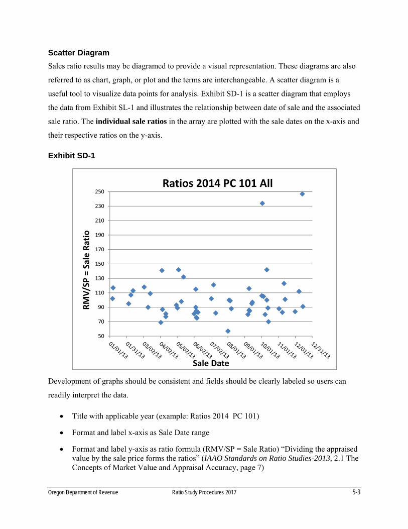
Oregon Department of Revenue Ratio Study Procedures 2017 5-3
Scatter Diagram
Sales ratio results may be diagramed to provide a visual representation. These diagrams are also
referred to as chart, graph, or plot and the terms are interchangeable. A scatter diagram is a
useful tool to visualize data points for analysis. Exhibit SD-1 is a scatter diagram that employs
the data from Exhibit SL-1 and illustrates the relationship between date of sale and the associated
sale ratio. The individual sale ratios in the array are plotted with the sale dates on the x-axis and
their respective ratios on the y-axis.
Exhibit SD-1
Development of graphs should be consistent and fields should be clearly labeled so users can
readily interpret the data.
Title with applicable year (example: Ratios 2014 PC 101)
Format and label x-axis as Sale Date range
Format and label y-axis as ratio formula (RMV/SP = Sale Ratio) “Dividing the appraised value by the sale price forms the ratios” (IAAO Standards on Ratio Studies-2013, 2.1 The Concepts of Market Value and Appraisal Accuracy, page 7)
50
70
90
110
130
150
170
190
210
230
250
RMV/SP = Sale Ratio
Sale Date
Ratios 2014 PC 101 All

Oregon Department of Revenue Ratio Study Procedures 2017 5-4
Outliers
Ratios in Exhibit SL-1 are sorted in ascending order. This grouping allows the analyst to readily
identify extreme ratios at either end of the array as compared with other ratios in the sales list.
These very low or very high ratios are often called outliers. Some outliers occur naturally; others
may be due to data entry error. In Exhibit SD-1, the two data points significantly separated from
the cluster of data are likely outliers.
Outliers require additional scrutiny to identify whether the sale is a non-market transaction and
may need to be trimmed or is an arm’s-length transaction and should remain in the study.
According to the IAAO, outlier ratios can result from any of the following:
1. An erroneous sale price
2. A non-market sale
3. Unusual market variability
4. A mismatch between the property sold and the property appraised
5. An error in the appraisal of an individual parcel
6. An error in the appraisal of a subgroup of parcels
7. Any of a variety of transcription or data handling errors
If an error can be corrected (for example, office input error), the sale could be left in the sales
list. However, leaving outlier sales in the data analysis can have a controlling influence over
statistical measures (e.g., mean, standard deviation, coefficient of variation, confidence interval).
When outliers are not representative of the general market, they should be trimmed from the
sales list using approved methods. If a trimming method is used to reject outlier ratios from the
sales list, include the method and reasoning in the ratio study report.
Arbitrarily trimming outliers based solely on their positioning in the ratio array is not an
acceptable procedure and is not supported by the Department of Revenue or the IAAO.
However, trimming of outliers using arbitrary limits, for example, eliminating all ratios less than 50 percent or greater than 150 percent, tends to distort results and should not be employed. (IAAO Standard on Ratio Studies-2013, Appendix B, B.3 Outlier Trimming, page 53)
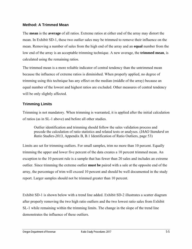
Oregon Department of Revenue Ratio Study Procedures 2017 5-5
Method: A Trimmed Mean
The mean is the average of all ratios. Extreme ratios at either end of the array may distort the
mean. In Exhibit SD-1, these two outlier sales may be trimmed to remove their influence on the
mean. Removing a number of sales from the high end of the array and an equal number from the
low end of the array is an acceptable trimming technique. A new average, the trimmed mean, is
calculated using the remaining ratios.
The trimmed mean is a more reliable indicator of central tendency than the untrimmed mean
because the influence of extreme ratios is diminished. When properly applied, no degree of
trimming using this technique has any effect on the median (middle of the array) because an
equal number of the lowest and highest ratios are excluded. Other measures of central tendency
will be only slightly affected.
Trimming Limits
Trimming is not mandatory. When trimming is warranted, it is applied after the initial calculation
of ratios (as in SL-1 above) and before all other studies.
Outlier identification and trimming should follow the sales validation process and precede the calculation of ratio statistics and related tests or analyses. (IAAO Standard on Ratio Studies-2013, Appendix B, B.1 Identification of Ratio Outliers, page 53)
Limits are set for trimming outliers. For small samples, trim no more than 10 percent. Equally
trimming the upper and lower five percent of the data creates a 10 percent trimmed mean. An
exception to the 10 percent rule is a sample that has fewer than 20 sales and includes an extreme
outlier. Since trimming the extreme outlier must be paired with a sale at the opposite end of the
array, the percentage of trim will exceed 10 percent and should be well documented in the study
report. Larger samples should not be trimmed greater than 10 percent.
Exhibit SD-1 is shown below with a trend line added. Exhibit SD-2 illustrates a scatter diagram
after properly removing the two high ratio outliers and the two lowest ratio sales from Exhibit
SL-1 while remaining within the trimming limits. The change in the slope of the trend line
demonstrates the influence of these outliers.
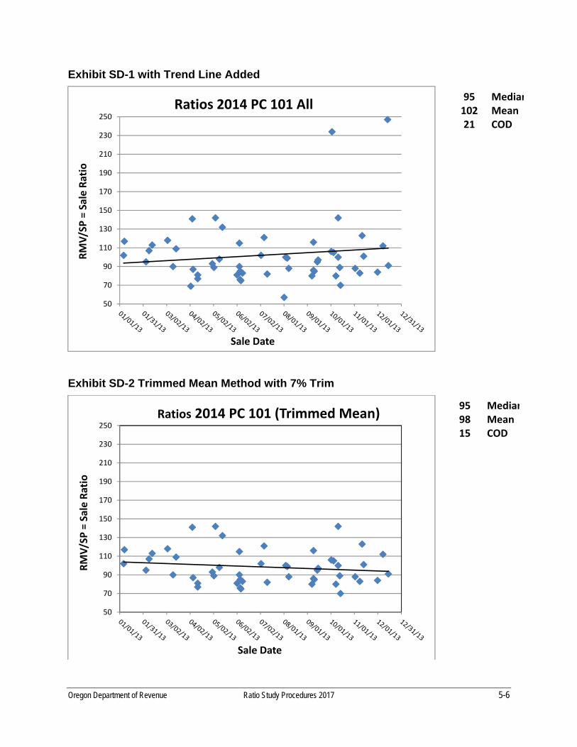
Oregon Department of Revenue Ratio Study Procedures 2017 5-6
Exhibit SD-1 with Trend Line Added
Exhibit SD-2 Trimmed Mean Method with 7% Trim
50
70
90
110
130
150
170
190
210
230
250
RMV/SP = Sale Ratio
Sale Date
Ratios 2014 PC 101 All
50
70
90
110
130
150
170
190
210
230
250
RMV/SP = Sale Ratio
Sale Date
Ratios 2014 PC 101 (Trimmed Mean)95 Median98 Mean15 COD
95 Median102 Mean21 COD
Oregon Department of Revenue Ratio Study Procedures 2017 5-7
Method: Interquartile Range Trimming
The other approved method for identifying extreme outliers is called Interquartile Range
(IQR). This trimming method is based on sound statistical theory and practice and is supported
by the Department of Revenue and the IAAO. Unlike the Trimmed Mean method, this analysis
does not depend on equal trimming from both ends of the array. This application is particularly
effective when data is skewed to one side. It adjusts the skewed data to reflect a more normal
distribution by computing trim boundaries which identify the outlier ratios. Dividing a list of
sales into quarters and statistically computing the trim boundaries requires several steps and is
best applied using a spreadsheet program. The steps are as follows:
1. Array ratios in ascending order. (In Exhibit SL-1 the ratios range from 57 to 247)
2. Identify the number of sales. (In Exhibit SL-1 there are 54 sales)
3. Identify the first trim boundary (quartile point) located between the first and second
quarter.
Formula to locate the boundary between the first and second quartile:
a. (0.25 x number of ratios) + 0.25
b. Example using Exhibit SL-1: (0.25 x 54 ratios) + 0.25 = 13.75
13.75 is three-quarters between the 13th and 14th ratio in the array of 54 sales
Ratio 13 = 83.00 and Ratio 14 = 84.00
Three-quarters between = (84.00 – 83.00) x 0.75 = 0.75
The first quartile point = 83.00 + 0.75 = 83.75
4. Identify the third trim boundary (quartile point) located between the third and fourth
quarter.
a. 0.75 x number of ratios) + 0.75
b. Example using Exhibit SL-1: (0.75 x 54 ratios) + 0.75 = 41.25
41.25 is one-quarter between the 41st and 42nd ratio in the array of 54 sales
Ratio 41 = 112.00 and Ratio 42 = 113.00
One-quarter between = (113.00 – 112.00) x 0.25 = 0.25
The third quartile point = 112.00 + 0.25 = 112.25
5. Compute the interquartile range
a. The distance between the third and first quartile = interquartile range
b. 112.25 – 83.75 = 28.5
Oregon Department of Revenue Ratio Study Procedures 2017 5-8
6. Establish the lower boundary
a. Lower trim point = first quartile − (interquartile range x 1.5)
b. 83.75 − (28.5 x 1.5) = 41.00
7. Establish the upper boundary
a. Upper trim point = third quartile + (interquartile range x 1.5)
b. 112.25 + (28.5 x 1.5) = 155.00
8. Outliers identified:
a. Any ratios that are less than 41.00
In Exhibit SL-1, there are no ratios that are less than 41.00
b. Any ratios that are greater than 155.00
In Exhibit SL-1, there are two ratios greater than 155.00 (234 and 247)
9. Remove identified outliers from the ratio array and calculate the central tendencies.
The exhibits below illustrate the trend line slope before and after the IQR trimming method is
applied.
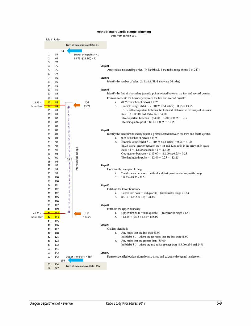
Oregon Department of Revenue Ratio Study Procedures 2017 5-9
Sale # Ratio
41
1 57 Lower trim point = 41
2 69 83.75 ‐ (28.5/2) = 41
3 70
4 75 Step #1
5 76 Array ratios in ascending order. (In Exhibit SL-1 the ratios range from 57 to 247)6 77
7 80 Step #2
8 80 Identify the number of sales. (In Exhibit SL-1 there are 54 sales)9 81
10 81 Step #3
11 82 Identify the first trim boundary (quartile point) located between the first and second quarter.
12 83 Formula to locate the boundary between the first and second quartile:13 83 a (0.25 x number of ratios) + 0.2514 84 b. Example using Exhibit SL-1: (0.25 x 54 ratios) + 0.25 = 13.7515 85 13.75 is three-quarters between the 13th and 14th ratio in the array of 54 sales16 85 Ratio 13 = 83.00 and Ratio 14 = 84.0017 86 Three-quarters between = (84.00 – 83.00) x 0.75 = 0.7518 87 The first quartile point = 83.00 + 0.75 = 83.7519 88
20 88 Step #4
21 89 Identify the third trim boundary (quartile point) located between the third and fourth quarter. 22 89 a. 0.75 x number of ratios) + 0.7523 90 b. Example using Exhibit SL-1: (0.75 x 54 ratios) + 0.75 = 41.2524 90 41.25 is one-quarter between the 41st and 42nd ratio in the array of 54 sales25 91 Ratio 41 = 112.00 and Ratio 42 = 113.0026 93 One-quarter between = (113.00 – 112.00) x 0.25 = 0.2527 95 The third quartile point = 112.00 + 0.25 = 112.2528 95
29 97 Step #5
30 98 Compute the interquartile range31 99 a. The distance between the third and first quartile = interquartile range
32 100 b. 112.25 – 83.75 = 28.5
33 100
34 101 Step #6
35 102 Establish the lower boundary36 102 a. Lower trim point = first quartile − (interquartile range x 1.5)37 105 b. 83.75 − (28.5 x 1.5) = 41.0038 106
39 107 Step #7
40 109 Establish the upper boundary41 112 a. Upper trim point = third quartile + (interquartile range x 1.5)42 113 b. 112.25 + (28.5 x 1.5) = 155.0043 115
44 116 Step #8
45 117 Outliers identified:46 118 a. Any ratios that are less than 41.0047 121 In Exhibit SL-1, there are no ratios that are less than 41.0048 123 b. Any ratios that are greater than 155.0049 132 In Exhibit SL-1, there are two ratios greater than 155.00 (234 and 247)50 141
51 142 Step #9
52 142 Upper trim point = 155 Remove identified outliers from the ratio array and calculate the central tendencies.155
53 234
54 247
Trim all sales below Ratio 41
Method: Interquartile Range TrimmingData from Exhibit SL‐1
Interquartile
Range
Trim all sales above Ratio 155
13.75 =
boundary
IQ1
IQ341.25 =
boundary
28.5
83.75
112.25

Oregon Department of Revenue Ratio Study Procedures 2017 5-10
Exhibit SD-1 with Trend Line Added
Exhibit SD-3 Interquartile Method with 4% Trim
50
70
90
110
130
150
170
190
210
230
250
RMV/SP = Sale Ratio
Sale Date
Ratios 2014 PC 101 All
50
70
90
110
130
150
170
190
210
230
250
RMV/SP = Sale Ratio
Sale Date
Ratios 2014 PC 101 (Interquartile Trimmed)
95 Median102 Mean21 COD
94 Median97 Mean16 COD
Oregon Department of Revenue Ratio Study Procedures 2017 5-11
Trimming Limits Specific to IQR
For some distributions, such as when the sample exhibits a high clustering around a specific ratio, the IQR outlier identification method is not appropriate. In such cases the IQR could be quite narrow, leading to the calculation of lower and upper boundaries for outliers and extremes that are quite close to the middle of the data. In such cases, ratios beyond those boundaries should not be automatically excluded, but instead reasonable judgment should be applied to exclude only true outliers or extremes. As one safeguard, analysts can refrain from automatically deleting any “outliers” or “extremes” inside the boundaries where 95 percent (two standard deviations) of the observations would be expected to lie, assuming a normal distribution of data. (IAAO Standard on Ratio Studies-2013, Appendix B, B.4 Trimming Limitations, page 54)
Trimming Recap
Trimming is not mandatory
When trimming, follow recognized procedures and show documentation
Trim before all other studies
Do not exceed trim limits and show documentation
Trimmed Mean Method: trim equal amounts from both ends of the ratio array
IQR Method: statistically robust; allows trimming of ratios in unequal numbers from the
extreme ends of an array, but certain conditions must be met

Oregon Department of Revenue Ratio Study Procedures 2017 6-1
SECTION 6
BASIC RATIO STATISTICS
Introduction
Knowledge of basic statistics is necessary to assemble a credible ratio study report. Some
statistical measures the analyst must be familiar with are median, mean, weighted mean,
geometric mean, and mode. These statistical measures infer where most of the data seems to be
concentrated in a dataset (sales list) and are referred to as central tendencies. These central
tendencies are derived from the arrayed ratios in the sales listings (sample). Ratios can be
expressed in decimal, percent, or whole number form.
There are several measures of central tendency that have proven to be reliable in ratio studies and
each has relative advantages and disadvantages. The three most applicable to ratio studies,
median, mean, and weighted mean, are required to complete the ratio study report. The goal is
to select one central tendency that best measures the RMV level for the study period.
Median is the middle of the array, influenced only by the position of the ratios in the
array, not by their values. The median is required to calculate the coefficient of dispersion
(COD - see Section 9).
Mean (Arithmetic Mean) is the simple average of the individual ratios in the sales array.
The mean is required to calculate the price related differential (PRD - see Section 9).
Weighted mean is derived by dividing the total of the current certified roll RMVs or
recalculated value of the sales by the total of the sale prices in the array and is required to
calculate the PRD.
Two additional measures of central tendency that may be used are geometric mean and mode.
Geometric mean is determined by multiplying all of the ratios in an array sequentially
and then taking the “-nth” root of this product.
Mode is the ratio that occurs in the ratio array most frequently.
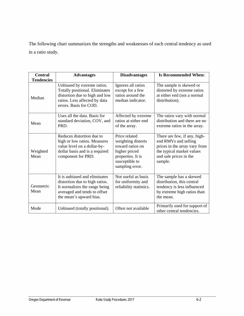
Oregon Department of Revenue Ratio Study Procedures 2017 6-2
The following chart summarizes the strengths and weaknesses of each central tendency as used
in a ratio study.
Central Tendencies
Advantages Disadvantages Is Recommended When:
Median
Unbiased by extreme ratios. Totally positional. Eliminates distortion due to high and low ratios. Less affected by data errors. Basis for COD.
Ignores all ratios except for a few ratios around the median indicator.
The sample is skewed or distorted by extreme ratios at either end (not a normal distribution).
Mean
Uses all the data. Basis for standard deviation, COV, and PRD.
Affected by extreme ratios at either end of the array.
The ratios vary with normal distribution and there are no extreme ratios in the array.
Weighted Mean
Reduces distortion due to high or low ratios. Measures value level on a dollar-by-dollar basis and is a required component for PRD.
Price related weighting distorts toward ratios on higher priced properties. It is susceptible to sampling error.
There are few, if any, high-end RMVs and selling prices in the array vary from the typical market values and sale prices in the sample.
Geometric Mean
It is unbiased and eliminates distortion due to high ratios. It normalizes the range being averaged and tends to offset the mean’s upward bias.
Not useful as basis for uniformity and reliability statistics.
The sample has a skewed distribution, this central tendency is less influenced by extreme high ratios than the mean.
Mode Unbiased (totally positional). Often not available Primarily used for support of other central tendencies.
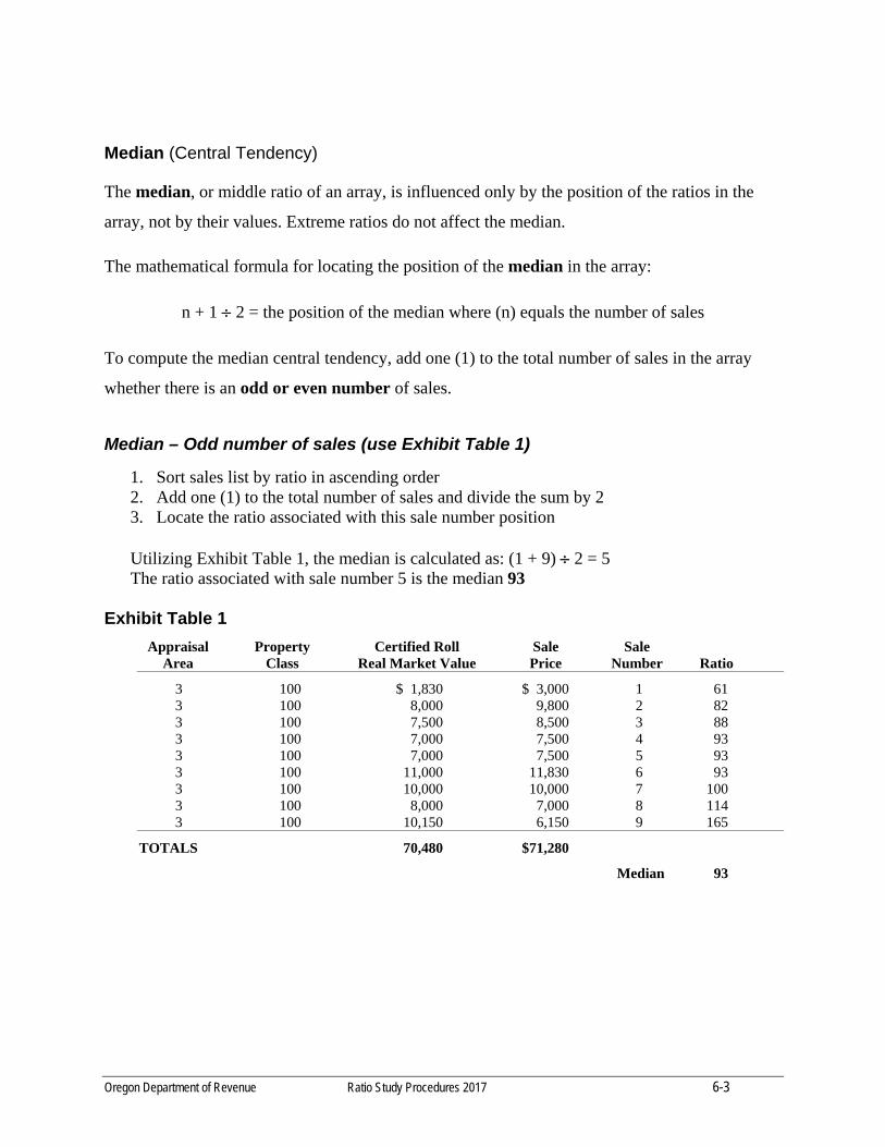
Oregon Department of Revenue Ratio Study Procedures 2017 6-3
Median (Central Tendency)
The median, or middle ratio of an array, is influenced only by the position of the ratios in the
array, not by their values. Extreme ratios do not affect the median.
The mathematical formula for locating the position of the median in the array:
n + 1 2 = the position of the median where (n) equals the number of sales
To compute the median central tendency, add one (1) to the total number of sales in the array
whether there is an odd or even number of sales.
Median – Odd number of sales (use Exhibit Table 1)
1. Sort sales list by ratio in ascending order 2. Add one (1) to the total number of sales and divide the sum by 2 3. Locate the ratio associated with this sale number position
Utilizing Exhibit Table 1, the median is calculated as: (1 + 9) 2 = 5
The ratio associated with sale number 5 is the median 93
Exhibit Table 1
Appraisal Property Certified Roll Sale Sale Area Class Real Market Value Price Number Ratio
3 100 $ 1,830 $ 3,000 1 61 3 100 8,000 9,800 2 82 3 100 7,500 8,500 3 88 3 100 7,000 7,500 4 93 3 100 7,000 7,500 5 93 3 100 11,000 11,830 6 93 3 100 10,000 10,000 7 100 3 100 8,000 7,000 8 114 3 100 10,150 6,150 9 165
TOTALS 70,480 $71,280
Median 93
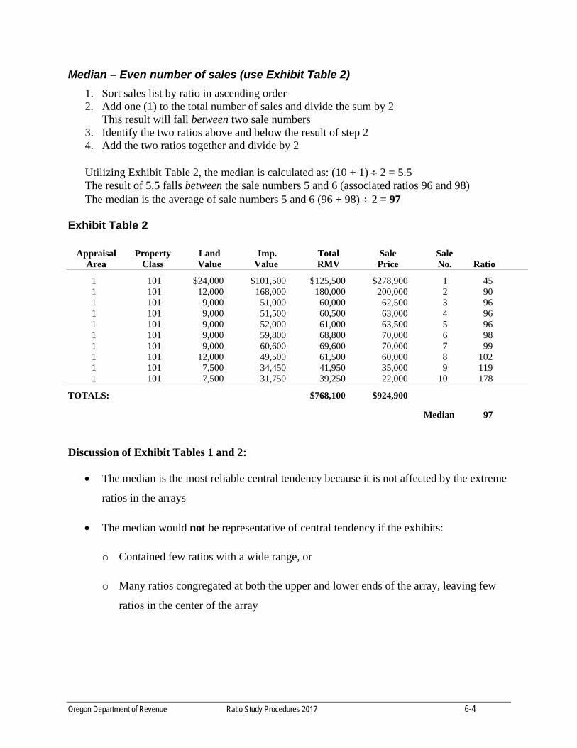
Oregon Department of Revenue Ratio Study Procedures 2017 6-4
Median – Even number of sales (use Exhibit Table 2)
1. Sort sales list by ratio in ascending order 2. Add one (1) to the total number of sales and divide the sum by 2 This result will fall between two sale numbers 3. Identify the two ratios above and below the result of step 2 4. Add the two ratios together and divide by 2
Utilizing Exhibit Table 2, the median is calculated as: (10 + 1) 2 = 5.5
The result of 5.5 falls between the sale numbers 5 and 6 (associated ratios 96 and 98) The median is the average of sale numbers 5 and 6 (96 + 98) 2 = 97
Exhibit Table 2
Appraisal Property Land Imp. Total Sale Sale Area Class Value Value RMV Price No. Ratio
1 101 $24,000 $101,500 $125,500 $278,900 1 45 1 101 12,000 168,000 180,000 200,000 2 90 1 101 9,000 51,000 60,000 62,500 3 96 1 101 9,000 51,500 60,500 63,000 4 96 1 101 9,000 52,000 61,000 63,500 5 96 1 101 9,000 59,800 68,800 70,000 6 98 1 101 9,000 60,600 69,600 70,000 7 99 1 101 12,000 49,500 61,500 60,000 8 102 1 101 7,500 34,450 41,950 35,000 9 119 1 101 7,500 31,750 39,250 22,000 10 178
TOTALS: $768,100 $924,900
Median 97
Discussion of Exhibit Tables 1 and 2:
The median is the most reliable central tendency because it is not affected by the extreme
ratios in the arrays
The median would not be representative of central tendency if the exhibits:
o Contained few ratios with a wide range, or
o Many ratios congregated at both the upper and lower ends of the array, leaving few
ratios in the center of the array
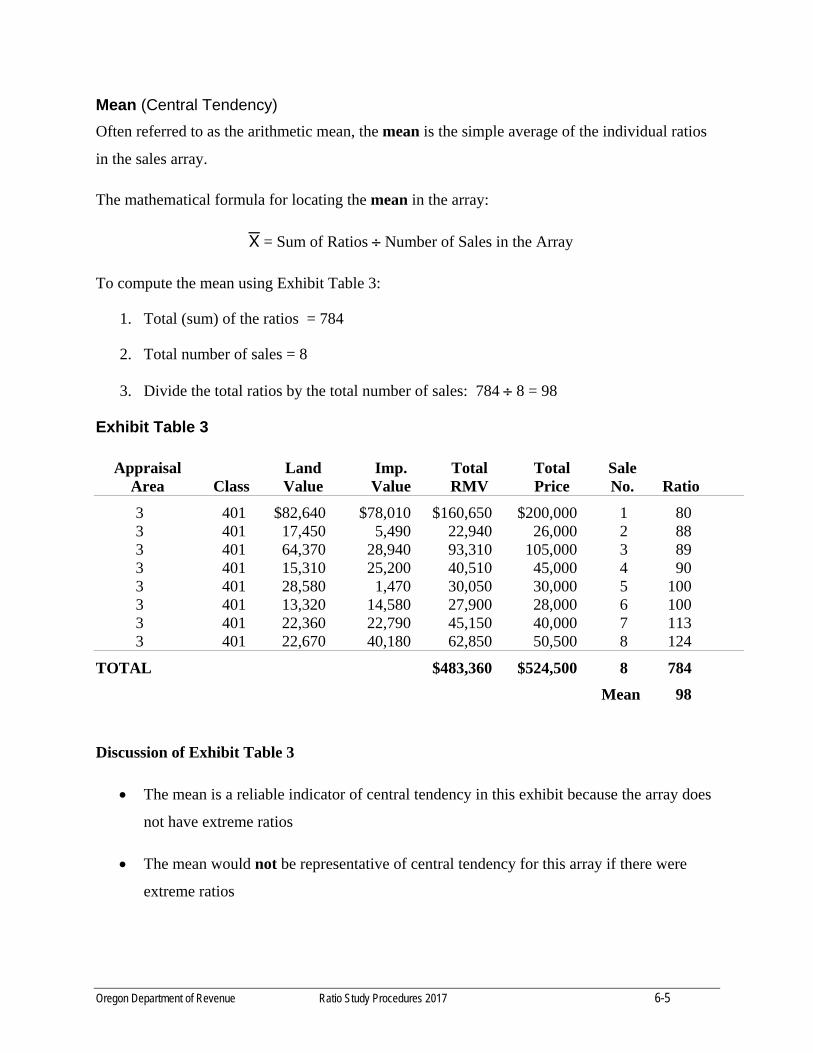
Oregon Department of Revenue Ratio Study Procedures 2017 6-5
Mean (Central Tendency)
Often referred to as the arithmetic mean, the mean is the simple average of the individual ratios
in the sales array.
The mathematical formula for locating the mean in the array:
= Sum of Ratios Number of Sales in the Array
To compute the mean using Exhibit Table 3:
1. Total (sum) of the ratios = 784
2. Total number of sales = 8
3. Divide the total ratios by the total number of sales: 784 8 = 98
Exhibit Table 3
Appraisal Land Imp. Total Total Sale Area Class Value Value RMV Price No. Ratio
3 401 $82,640 $78,010 $160,650 $200,000 1 80 3 401 17,450 5,490 22,940 26,000 2 88 3 401 64,370 28,940 93,310 105,000 3 89 3 401 15,310 25,200 40,510 45,000 4 90 3 401 28,580 1,470 30,050 30,000 5 100 3 401 13,320 14,580 27,900 28,000 6 100 3 401 22,360 22,790 45,150 40,000 7 113 3 401 22,670 40,180 62,850 50,500 8 124
TOTAL $483,360 $524,500 8 784
Mean 98
Discussion of Exhibit Table 3
The mean is a reliable indicator of central tendency in this exhibit because the array does
not have extreme ratios
The mean would not be representative of central tendency for this array if there were
extreme ratios
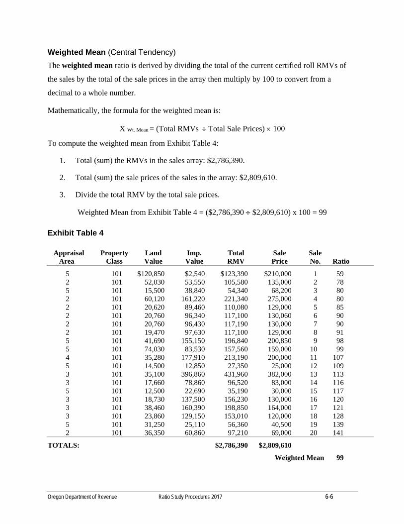
Oregon Department of Revenue Ratio Study Procedures 2017 6-6
Weighted Mean (Central Tendency)
The weighted mean ratio is derived by dividing the total of the current certified roll RMVs of
the sales by the total of the sale prices in the array then multiply by 100 to convert from a
decimal to a whole number.
Mathematically, the formula for the weighted mean is:
X Wt. Mean = (Total RMVs Total Sale Prices) 100
To compute the weighted mean from Exhibit Table 4:
1. Total (sum) the RMVs in the sales array: $2,786,390.
2. Total (sum) the sale prices of the sales in the array: $2,809,610.
3. Divide the total RMV by the total sale prices.
Weighted Mean from Exhibit Table 4 = ($2,786,390 $2,809,610) x 100 = 99
Exhibit Table 4
Appraisal Property Land Imp. Total Sale Sale Area Class Value Value RMV Price No. Ratio
5 101 $120,850 $2,540 $123,390 $210,000 1 59 2 101 52,030 53,550 105,580 135,000 2 78 5 101 15,500 38,840 54,340 68,200 3 80 2 101 60,120 161,220 221,340 275,000 4 80 2 101 20,620 89,460 110,080 129,000 5 85 2 101 20,760 96,340 117,100 130,060 6 90 2 101 20,760 96,430 117,190 130,000 7 90 2 101 19,470 97,630 117,100 129,000 8 91 5 101 41,690 155,150 196,840 200,850 9 98 5 101 74,030 83,530 157,560 159,000 10 99 4 101 35,280 177,910 213,190 200,000 11 107 5 101 14,500 12,850 27,350 25,000 12 109 3 101 35,100 396,860 431,960 382,000 13 113 3 101 17,660 78,860 96,520 83,000 14 116 5 101 12,500 22,690 35,190 30,000 15 117 3 101 18,730 137,500 156,230 130,000 16 120 3 101 38,460 160,390 198,850 164,000 17 121 3 101 23,860 129,150 153,010 120,000 18 128 5 101 31,250 25,110 56,360 40,500 19 139 2 101 36,350 60,860 97,210 69,000 20 141
TOTALS: $2,786,390 $2,809,610
Weighted Mean 99

Oregon Department of Revenue Ratio Study Procedures 2017 6-7
Discussion of Exhibit Table 4:
The weighted mean is the best selected central tendency because it takes into
consideration the ratios of the sales with large dollar values that are evenly distributed
throughout the sample
The weighted mean weighs each ratio in proportion to its sale price, whereas the mean
and median give equal weight to each sale price
The weighted mean would not be representative of central tendency if the exhibit:
o Contained several high-value properties with relatively low or high ratios which
could indicate a sampling error
o Had higher value properties concentrated at either end of the array
The three primary measures of central tendency are illustrated in Exhibit Table 5 and is followed
by a discussion of the best indicator selection.
Exhibit Table 5
Property Class 101 in MA 1
Appraisal Property Land Imp. Total Sale Sale Area Class Value Value RMV Price No. Ratio
1 101 $24,000 $101,500 $125,500 $150,000 1 84 1 101 12,000 168,000 180,000 200,000 2 90 1 101 9,000 51,000 60,000 62,500 3 96 1 101 9,000 51,500 60,500 63,000 4 96 1 101 9,000 52,000 61,000 63,500 5 96 1 101 9,000 59,800 68,800 70,000 6 98 1 101 9,000 60,600 69,600 70,000 7 99 1 101 12,000 49,500 61,500 60,000 8 102 1 101 7,500 34,450 41,950 35,000 9 119 1 101 7,500 31,750 39,250 30,000 10 130
TOTALS: $768,100 $804,000 1,010
MEAN 101 WEIGHTED MEAN 96 MEDIAN 97
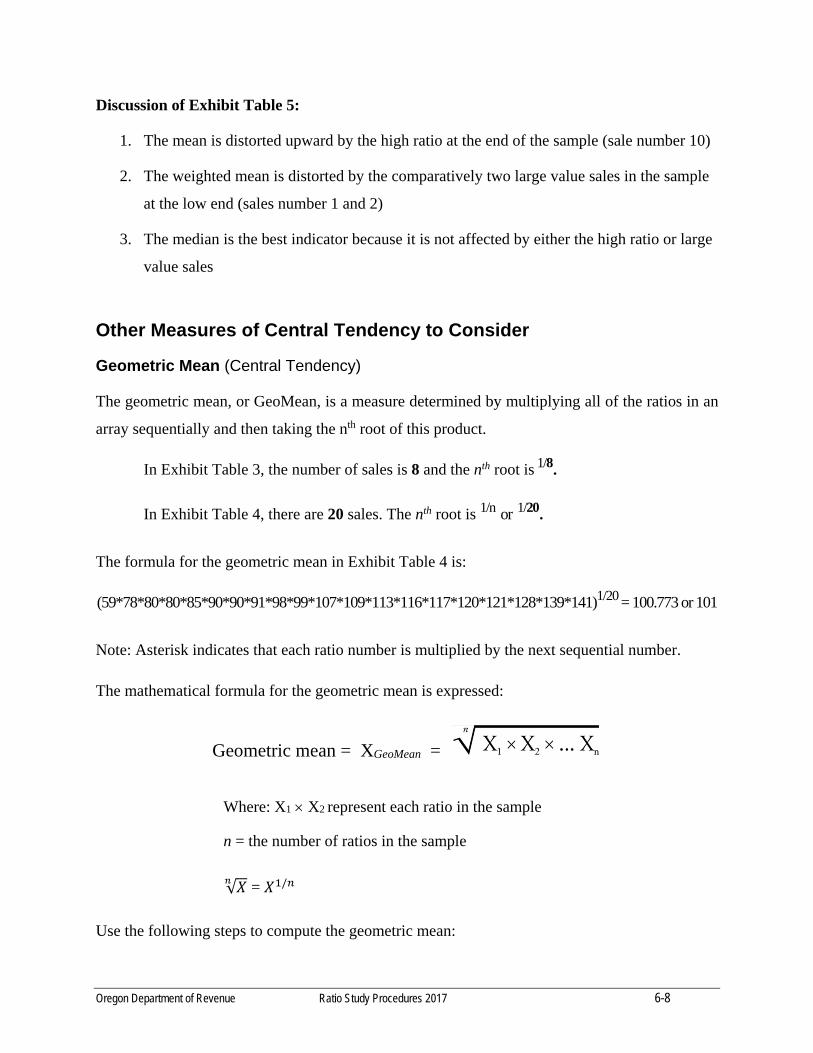
Oregon Department of Revenue Ratio Study Procedures 2017 6-8
Discussion of Exhibit Table 5:
1. The mean is distorted upward by the high ratio at the end of the sample (sale number 10)
2. The weighted mean is distorted by the comparatively two large value sales in the sample
at the low end (sales number 1 and 2)
3. The median is the best indicator because it is not affected by either the high ratio or large
value sales
Other Measures of Central Tendency to Consider
Geometric Mean (Central Tendency)
The geometric mean, or GeoMean, is a measure determined by multiplying all of the ratios in an
array sequentially and then taking the nth root of this product.
In Exhibit Table 3, the number of sales is 8 and the nth root is 1/8.
In Exhibit Table 4, there are 20 sales. The nth root is 1/n or 1/20.
The formula for the geometric mean in Exhibit Table 4 is:
(59*78*80*80*85*90*90*91*98*99*107*109*113*116*117*120*121*128*139*141)1/20 = 100.773 or 101
Note: Asterisk indicates that each ratio number is multiplied by the next sequential number.
The mathematical formula for the geometric mean is expressed:
Geometric mean = XGeoMean =
Where: X1 X2 represent each ratio in the sample
n = the number of ratios in the sample
√ = /
Use the following steps to compute the geometric mean:
Oregon Department of Revenue Ratio Study Procedures 2017 6-9
1. Compute the ratio for each sale in the array
2. Multiply each ratio by the next ratio in the array (this will be a very large number)
3. Take the nth root of the ultimate product (in Exhibit Table 4 since there are 20 ratios, n =
20 and the nth =1/20), rounded to a whole number
Discussion of geometric mean
The geometric mean may be applicable when the sample is skewed with high ratios
The geometric mean, like the median, is not as susceptible to distortion by extreme high
ratios as the mean or the weighted mean
Unless every ratio in the sample is identical, the geometric mean will be less than the
mean
If the ratios vary widely, the geometric mean may lie considerably below the other
measures of central tendency
The geometric mean is not useful as a basis for calculating reliability statistics
Mode (Central Tendency)
The mode is the ratio that occurs most frequently in the ratio array. There is no formula for this
calculation. The mode, like the median, is a positional measure.
The steps are:
1. Sort the ratios in ascending order
2. Count how many of each ratio
3. The ratio that appears most often is the mode
4. Having two modes is bimodal. More than two modes are multimodal
In Exhibit Table 5, the ratio of 96 appears most often and is the mode.
In Exhibit Table 4, the ratios of 80 and 90 appear the most frequently and both occur an equal
number of times. This indicates that the array in Exhibit Table 4 is bimodal.

Oregon Department of Revenue Ratio Study Procedures 2017 7-1
SECTION 7
ANALYSIS: CHANGE IN MARKET
CONDITIONS OVER TIME
Introduction
Market conditions change over time. Statute establishes an assessment date of January 1, at 1:00
a.m., and requires assessors to value property as of that date [ORS 308.210(1)]. Property sales
occur throughout the entire year and prices must be adjusted to reflect the real market value of
the property as if the sale occurred on the assessment date.
Assessors are also required by statute to annually collect sales for the assessment year from
January 1 to December 31. Collected sales are placed in a database for confirmation and coding
of sales. This database need not be entirely separate from the assessment roll or other databases
maintained by the county provided the analyst is able to store, view, and retrieve the necessary
information. The sales from this file can be used to investigate, measure, and adjust sale prices
for change in market conditions.
Fluctuating market conditions may create the need to apply an adjustment to sales prices that
occurred during the sales year. Although the adjustment is often called a time adjustment, time
itself is not the reason for the adjustment; it is the movement of value over time. The adjustment
is expressed as a percentage of increase or decrease to sales prices to reflect what the property
would have sold for as of the assessment date.
A January through December ratio study, as required by statute (ORS 309.200), without a time
adjustment, reflects the market at a mid-point of the sales year, usually July. When a time study
reveals a change in market conditions is warranted, but is not applied, the values are not
adjusted to the January 1 assessment date.
Any adjustment for change in market conditions over time should be based on well supported
analysis of the data. If the investigation and analysis indicate market conditions have not
changed over time, an adjustment to sale prices for change over time is not required. Regardless
Oregon Department of Revenue Ratio Study Procedures 2017 7-2
of the adjustment conclusion, the supporting study and objective rationale is required in the ratio
study report.
Time adjustments are applied in the beginning stages of the study(s) and affect all further
analysis and conclusions.
Trends
Assessors are required to investigate annual trends in real estate market values for ratio purposes
(ORS 309.200). Within the annual trends there may be seasonal trends and sometimes short-term
trends that suggest variable rates of change occurring throughout the year. The analyst must
recognize the types of trends affecting the current market in order to research and properly adjust
sale prices to the assessment date.
Types of Trends
A trend is the general movement over time of a statistically measureable change. Sale prices
reflect preferences in the market and may be influenced by local, regional, national, or world-
wide trends. Some familiar trends include:
Annual Trend
This is the rate of change from one year to the next or any 12-month period.
Cost Trend
The rate of change in construction costs.
Economic Trend
A general trend logically based on economic factors.
Long-Term Trend
The rate of change over a number of years is the Long-Term Trend. Some industries such as
housing or wood products experience dynamics that may or may not change rapidly and are
cyclical in nature. These industry-wide changes may reflect changes in supply (resource
shortage) and demand (demographic change).
Market Trend
This is the rate of change of market prices for specific classes of properties, such as multi-family

Oregon Department of Revenue Ratio Study Procedures 2017 7-3
residential, commercial, etc. Market trends are often set by or follow local, statewide, or regional
economics.
Seasonal Trend
Seasonal trend is a rate of change over a few specific months. This would also include winter use
areas, summer use areas; financial reporting quarterly periods, etc.
Seasonal Variation
The seasonal variation is a consistent relationship between an annual trend and a seasonal trend.
Short-Term Trend
Rate of change calculated over a few months or weeks. This may be used to determine the
direction of the market at a point in time.
Examining Market Trends
After the sales list is trimmed, the next step is to determine if there is an identifiable trend in
property sale prices over the assessment year or the range of the study period (monthly,
quarterly, annually, or multi-year). The two main methods of examining the market are Ratio
Analysis and Direct Sales Analysis. Ratio Analysis examines the relationship between the roll
value and the sale price and utilizes the techniques of direct calculation and mid-point. Direct
Sales Analysis studies compare the relationship of sales prices of the same (double) or highly
similar (paired) properties over a period of time (annual, quarter, month).
I. Ratio Analysis
a. Direct Calculation
b. Mid-point
II. Direct Sales Analysis a. Double sales
b. Paired sales
The following table, Exhibit SL-2, is the sales array from Section 5 (Ratio Calculation, Outliers,
and Trimming), after applying the Trimmed Mean Method. The sales list is trimmed from 54 to
50 sales; two high ratio outliers were trimmed as well as two sales from the other end of the
array according to the approved method. This table will be used to demonstrate techniques of
Ratio Analysis.
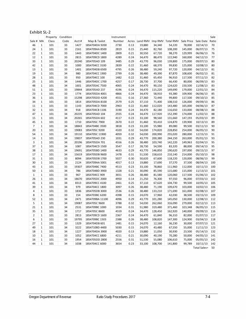
Oregon Department of Revenue Ratio Study Procedures 2017 7-4
Sale # MA
Property
Class
Condition
Code Acct # Map & Taxlot
Instrument
Number Acres Land RMV Imp RMV Total RMV Sale Price Sale Date
Sale
Ratio
46 1 101 33 1427 18S4704DA 9200 2730 0.13 19,880 34,340 54,220 78,000 10/14/13 70
24 1 101 33 2161 18S4709AA 8500 2819 0.15 25,440 82,760 108,200 145,000 06/07/13 75
22 1 101 33 1443 18S4704DC 1400 2809 0.21 30,550 67,720 98,270 129,999 06/06/13 76
12 1 101 33 2815 18S4709CD 1800 4289 0.24 34,470 88,470 122,940 160,000 04/12/13 77
33 1 101 33 20240 18S4705AD 109 3485 0.29 43,770 96,030 139,800 175,000 09/07/13 80
42 1 101 33 1000 18S4704CC 3100 2839 0.22 31,460 68,370 99,830 125,000 10/08/13 80
13 1 101 33 1401 18S4704DB 6500 4795 0.26 38,480 59,240 97,720 120,000 04/12/13 81
19 1 101 34 980 18S4704CC 1900 2799 0.26 38,480 49,390 87,870 108,600 06/02/13 81
28 1 101 33 950 18S4704CC 100 1482 0.22 31,460 65,450 96,910 117,500 07/11/13 82
25 1 101 34 1446 18S4704DC 1700 4257 0.17 28,730 37,700 66,430 80,000 06/09/13 83
48 1 101 34 1601 18S4705AC 7500 4065 0.24 34,470 90,150 124,620 150,500 11/08/13 83
51 1 101 33 19844 18S4705AD 237 4196 0.24 34,470 115,220 149,690 179,000 12/01/13 84
23 1 101 33 1774 18S4705DA 4001 4866 0.24 34,470 58,910 93,380 109,900 06/06/13 85
36 1 101 33 15298 18S4705DD 4200 4551 0.16 27,360 72,440 99,800 117,500 09/10/13 85
34 1 101 33 1814 18S4705DA 8100 2579 0.25 37,110 71,400 108,510 126,000 09/09/13 86
11 1 101 33 1143 18S4704CD 7000 2963 0.22 31,460 112,020 143,480 165,000 04/06/13 87
32 1 101 34 918 18S4704CB 1106 3190 0.24 34,470 82,180 116,650 133,000 08/08/13 88
47 1 101 34 20235 18S4705AD 104 2555 0.24 34,470 117,920 152,390 174,000 11/02/13 88
15 1 101 34 20265 18S4705DA 602 4117 0.23 33,100 98,560 131,660 147,193 05/03/13 89
45 1 101 33 1710 18S4705C 7900 2670 0.22 31,460 93,410 124,870 139,900 10/13/13 89
7 1 101 34 18843 18S4704BC 3500 3818 0.23 33,100 55,980 89,080 99,500 03/11/13 90
20 1 101 33 19083 18S4705C 9200 4320 0.32 54,030 174,820 228,850 254,000 06/05/13 90
54 1 101 34 19110 18S4705C 11900 4059 0.32 54,030 200,990 255,020 280,000 12/15/13 91
14 1 101 34 19837 18S4705AD 230 1031 0.29 43,770 200,380 244,150 263,000 05/01/13 93
3 1 101 34 20196 18S4705DA 701 4556 0.26 38,480 103,740 142,220 149,963 02/04/13 95
37 1 101 34 1087 18S4704CD 1500 3547 0.17 28,730 54,590 83,320 88,000 09/14/13 95
38 1 101 34 19691 18S4705BD 1400 4633 0.29 43,770 146,850 190,620 197,000 09/15/13 97
17 1 101 34 15619 18S4705DB 9600 1478 0.31 51,530 158,610 210,140 214,000 05/10/13 98
31 1 101 33 8094 18S4705DB 1700 5027 0.30 50,620 67,600 118,220 120,000 08/06/13 99
30 1 101 33 2124 18S4709AA 5001 4017 0.13 19,880 17,690 37,570 37,500 08/04/13 100
43 1 101 33 19307 18S4704BC 7400 4513 0.23 33,100 78,860 111,960 112,000 10/11/13 100
50 1 101 34 786 18S4704BD 3900 1328 0.21 30,090 85,590 115,680 115,000 11/13/13 101
1 1 101 33 967 18S4704CC 909 3651 0.26 38,480 81,580 120,060 117,500 01/06/13 102
26 1 101 34 18670 18S4705DC 2000 4950 0.14 21,250 76,300 97,550 96,000 07/03/13 102
41 1 101 34 8313 18S4709CC 4100 2461 0.25 37,110 67,620 104,730 99,500 10/05/13 105
39 1 101 34 979 18S4704CC 1800 3097 0.26 38,480 71,190 109,670 103,000 10/02/13 106
4 1 101 33 1836 18S4705DB 3000 2536 0.26 38,480 133,210 171,690 161,000 02/08/13 107
8 1 101 33 154 18S4703BC 6200 4398 0.15 24,070 17,960 42,030 38,500 03/15/13 109
52 1 101 34 2471 18S4709BA 11100 4096 0.29 43,770 101,280 145,050 130,000 12/08/13 112
5 1 101 34 19087 18S4705C 9600 3788 0.32 54,030 262,060 316,090 279,000 02/12/13 113
21 1 101 34 2531 18S4709BC 1000 1034 0.31 51,980 319,480 371,460 323,348 06/05/13 115
35 1 101 34 1717 18S4705C 8600 4559 0.24 34,470 128,450 162,920 140,000 09/09/13 116
2 1 101 33 2813 18S4709CD 1600 2367 0.24 34,470 61,840 96,310 82,000 01/07/13 117
6 1 101 33 19795 18S4709BC 1503 2388 0.26 38,480 108,820 147,300 124,900 03/04/13 118
27 1 101 33 1329 18S4704DB 601 1481 0.15 24,070 12,160 36,230 30,000 07/07/13 121
49 1 101 34 3222 18S4710BD 4400 5030 0.15 24,070 43,480 67,550 55,000 11/11/13 123
18 1 101 34 1227 18S4704DA 3900 4020 0.13 19,880 11,050 30,930 23,500 05/14/13 132
10 1 101 33 1052 18S4704CC 6800 4211 0.21 30,090 40,190 70,280 50,000 04/05/13 141
16 1 101 33 1954 18S4705DD 2800 2556 0.31 51,530 55,080 106,610 75,000 05/05/13 142
44 1 101 34 1038 18S4704CC 6000 3654 0.23 33,100 108,700 141,800 99,789 10/11/13 142
Total Sales= 50
Exhibit SL‐2
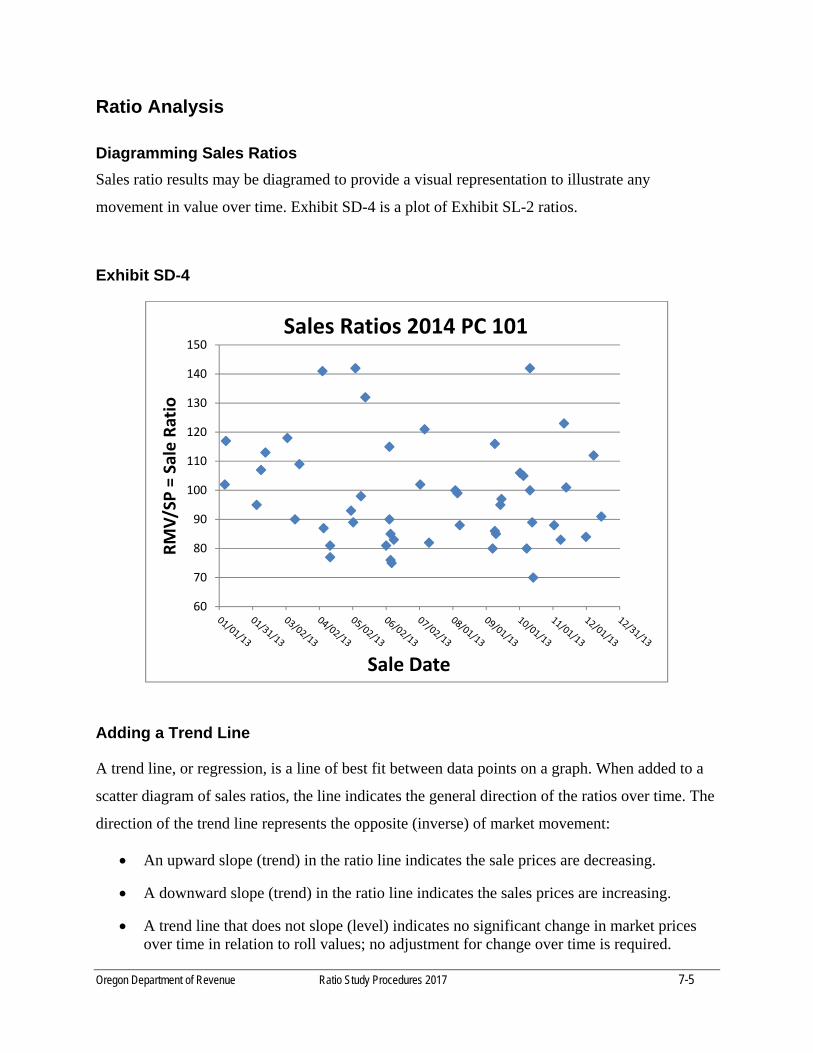
Oregon Department of Revenue Ratio Study Procedures 2017 7-5
Ratio Analysis
Diagramming Sales Ratios
Sales ratio results may be diagramed to provide a visual representation to illustrate any
movement in value over time. Exhibit SD-4 is a plot of Exhibit SL-2 ratios.
Exhibit SD-4
Adding a Trend Line
A trend line, or regression, is a line of best fit between data points on a graph. When added to a
scatter diagram of sales ratios, the line indicates the general direction of the ratios over time. The
direction of the trend line represents the opposite (inverse) of market movement:
An upward slope (trend) in the ratio line indicates the sale prices are decreasing.
A downward slope (trend) in the ratio line indicates the sales prices are increasing.
A trend line that does not slope (level) indicates no significant change in market prices over time in relation to roll values; no adjustment for change over time is required.
60
70
80
90
100
110
120
130
140
150
RMV/SP = Sale Ratio
Sale Date
Sales Ratios 2014 PC 101
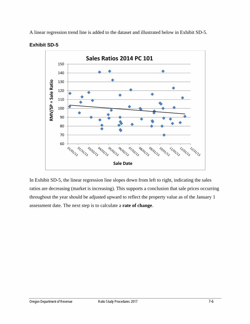
Oregon Department of Revenue Ratio Study Procedures 2017 7-6
A linear regression trend line is added to the dataset and illustrated below in Exhibit SD-5.
Exhibit SD-5
In Exhibit SD-5, the linear regression line slopes down from left to right, indicating the sales
ratios are decreasing (market is increasing). This supports a conclusion that sale prices occurring
throughout the year should be adjusted upward to reflect the property value as of the January 1
assessment date. The next step is to calculate a rate of change.
60
70
80
90
100
110
120
130
140
150
RMV/SP = Sale Ratio
Sale Date
Sales Ratios 2014 PC 101

Oregon Department of Revenue Ratio Study Procedures 2017 7-7
Determining the Rate of Change over Time
Exhibit SD-6
Ratio Analysis: Direct Calculation Applied on an Annual Basis
One example of determining the overall change in the market over time is to identify and
compare the intersection of the regression line with the y-axis as of the beginning and ending of
the study period using the inverse ratio technique.
In Exhibit SD-6, the trend line on the chart slopes downward indicating roll values at the end of
the year represent a smaller portion of sale prices than they did at the beginning of the year (sale
prices are increasing).
The extended regression line intersects the y-axis at the beginning of the period (January 1) at the
ratio point of 104 and intersects the y-axis at the end of the period (December 31) at the ratio
point 93. It is evident that a change in market conditions occurred over the year. In order to
compute an adjustment factor, use the following steps:
Steps to calculate a factor to adjust sale prices to the assessment date (Exhibit SD-6 data):
1. Extend the ratio regression line and identify the y-axis intersection points as of the
beginning (104%) and the ending (93%) of the ratio year.
60
70
80
90
100
110
120
130
140
150RMV/SP = Sale Ratio
Sale Date
Sales Ratios 2014 PC 101
93
104
Oregon Department of Revenue Ratio Study Procedures 2017 7-8
2. Compute the amount of change from the ending point to the beginning point of the
period (104% - 93% = 11%). This is not the adjustment factor.
3. Compute an annual change factor. The difference between the December 31 sale prices
which represent 100% of market value for the assessment date and the change over the
period (11%) is the amount of end of year price represented by a beginning of year sale
(100% -11% = 89%)
When the market is increasing, subtract the amount of change from 100%
When the market is decreasing, add the amount of change to 100%
4. Calculate an annual adjustment factor by dividing the amount from step 3 into 100%
(100% ÷ 89% = 112%)
5. Step 4 indicates the amount a beginning year sale must be adjusted to represent end of
year prices. Subtract 100% from the amount in step 4 to arrive at the overall adjustment
for the year
(112% - 100% = 12%)
6. Determine an intermediate period adjustment factor. Divide the overall adjustment for the
year by the number of periods (months, quarters). To arrive at the intermediate
adjustment factor on a monthly basis, divide the overall adjustment factor for the year
from step 5 by the number of months in a year
(12% ÷ 12 = 1% per month)
The conclusion of the rate of change per month is used to adjust sale prices on a monthly basis
from the date of sale to the target January 1 assessment date.
Example: A property sold for $200,000 in May
1. Determine the monthly adjustment factor (1.0% per month from above)
2. Determine the number of months between the sale date and the assessment date: There are 8 months between the sale date and the assessment date: May, June, July, August, September, October, November, December
3. Determine the total adjustment factor for this sale: The number of months multiplied by the monthly adjustment factor 8 x 1.0 = 8.0%

Oregon Department of Revenue Ratio Study Procedures 2017 7-9
4. Apply the total adjustment factor to the sale price to find the total adjustment: 200,000 x 8% = 16,000
5. Add the total adjustment to the sale price to arrive at the adjusted sale price: 200,000 + 16,000 = 216,000 The adjusted sale price would be $216,000
Steps 4 and 5 could be combined and expressed as: 200,000 x 108%.
It must be emphasized this technique of applying a linear regression analysis assumes property
values change by a constant percentage each month throughout the year.
In Exhibit SL-3, the sale prices are adjusted by a monthly rate. Market area studies will use the
resulting adjusted sale prices as the baseline for analysis.
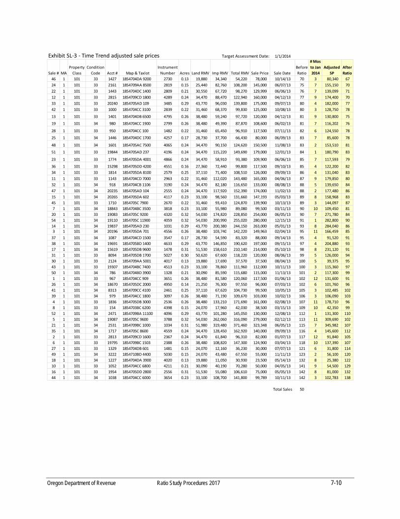
Oregon Department of Revenue Ratio Study Procedures 2017 7-10
1/1/2014
Sale # MA
Property
Class
Condition
Code Acct # Map & Taxlot
Instrument
Number Acres Land RMV Imp RMV Total RMV Sale Price Sale Date
Before
Ratio
# Mos
to Jan
2014
Adjusted
SP
After
Ratio
46 1 101 33 1427 18S4704DA 9200 2730 0.13 19,880 34,340 54,220 78,000 10/14/13 70 3 80,340 67
24 1 101 33 2161 18S4709AA 8500 2819 0.15 25,440 82,760 108,200 145,000 06/07/13 75 7 155,150 70
22 1 101 33 1443 18S4704DC 1400 2809 0.21 30,550 67,720 98,270 129,999 06/06/13 76 7 139,099 71
12 1 101 33 2815 18S4709CD 1800 4289 0.24 34,470 88,470 122,940 160,000 04/12/13 77 9 174,400 70
33 1 101 33 20240 18S4705AD 109 3485 0.29 43,770 96,030 139,800 175,000 09/07/13 80 4 182,000 77
42 1 101 33 1000 18S4704CC 3100 2839 0.22 31,460 68,370 99,830 125,000 10/08/13 80 3 128,750 78
13 1 101 33 1401 18S4704DB 6500 4795 0.26 38,480 59,240 97,720 120,000 04/12/13 81 9 130,800 75
19 1 101 34 980 18S4704CC 1900 2799 0.26 38,480 49,390 87,870 108,600 06/02/13 81 7 116,202 76
28 1 101 33 950 18S4704CC 100 1482 0.22 31,460 65,450 96,910 117,500 07/11/13 82 6 124,550 78
25 1 101 34 1446 18S4704DC 1700 4257 0.17 28,730 37,700 66,430 80,000 06/09/13 83 7 85,600 78
48 1 101 34 1601 18S4705AC 7500 4065 0.24 34,470 90,150 124,620 150,500 11/08/13 83 2 153,510 81
51 1 101 33 19844 18S4705AD 237 4196 0.24 34,470 115,220 149,690 179,000 12/01/13 84 1 180,790 83
23 1 101 33 1774 18S4705DA 4001 4866 0.24 34,470 58,910 93,380 109,900 06/06/13 85 7 117,593 79
36 1 101 33 15298 18S4705DD 4200 4551 0.16 27,360 72,440 99,800 117,500 09/10/13 85 4 122,200 82
34 1 101 33 1814 18S4705DA 8100 2579 0.25 37,110 71,400 108,510 126,000 09/09/13 86 4 131,040 83
11 1 101 33 1143 18S4704CD 7000 2963 0.22 31,460 112,020 143,480 165,000 04/06/13 87 9 179,850 80
32 1 101 34 918 18S4704CB 1106 3190 0.24 34,470 82,180 116,650 133,000 08/08/13 88 5 139,650 84
47 1 101 34 20235 18S4705AD 104 2555 0.24 34,470 117,920 152,390 174,000 11/02/13 88 2 177,480 86
15 1 101 34 20265 18S4705DA 602 4117 0.23 33,100 98,560 131,660 147,193 05/03/13 89 8 158,968 83
45 1 101 33 1710 18S4705C 7900 2670 0.22 31,460 93,410 124,870 139,900 10/13/13 89 3 144,097 87
7 1 101 34 18843 18S4704BC 3500 3818 0.23 33,100 55,980 89,080 99,500 03/11/13 90 10 109,450 81
20 1 101 33 19083 18S4705C 9200 4320 0.32 54,030 174,820 228,850 254,000 06/05/13 90 7 271,780 84
54 1 101 34 19110 18S4705C 11900 4059 0.32 54,030 200,990 255,020 280,000 12/15/13 91 1 282,800 90
14 1 101 34 19837 18S4705AD 230 1031 0.29 43,770 200,380 244,150 263,000 05/01/13 93 8 284,040 863 1 101 34 20196 18S4705DA 701 4556 0.26 38,480 103,740 142,220 149,963 02/04/13 95 11 166,459 85
37 1 101 34 1087 18S4704CD 1500 3547 0.17 28,730 54,590 83,320 88,000 09/14/13 95 4 91,520 91
38 1 101 34 19691 18S4705BD 1400 4633 0.29 43,770 146,850 190,620 197,000 09/15/13 97 4 204,880 93
17 1 101 34 15619 18S4705DB 9600 1478 0.31 51,530 158,610 210,140 214,000 05/10/13 98 8 231,120 91
31 1 101 33 8094 18S4705DB 1700 5027 0.30 50,620 67,600 118,220 120,000 08/06/13 99 5 126,000 94
30 1 101 33 2124 18S4709AA 5001 4017 0.13 19,880 17,690 37,570 37,500 08/04/13 100 5 39,375 95
43 1 101 33 19307 18S4704BC 7400 4513 0.23 33,100 78,860 111,960 112,000 10/11/13 100 3 115,360 97
50 1 101 34 786 18S4704BD 3900 1328 0.21 30,090 85,590 115,680 115,000 11/13/13 101 2 117,300 99
1 1 101 33 967 18S4704CC 909 3651 0.26 38,480 81,580 120,060 117,500 01/06/13 102 12 131,600 91
26 1 101 34 18670 18S4705DC 2000 4950 0.14 21,250 76,300 97,550 96,000 07/03/13 102 6 101,760 96
41 1 101 34 8313 18S4709CC 4100 2461 0.25 37,110 67,620 104,730 99,500 10/05/13 105 3 102,485 102
39 1 101 34 979 18S4704CC 1800 3097 0.26 38,480 71,190 109,670 103,000 10/02/13 106 3 106,090 103
4 1 101 33 1836 18S4705DB 3000 2536 0.26 38,480 133,210 171,690 161,000 02/08/13 107 11 178,710 96
8 1 101 33 154 18S4703BC 6200 4398 0.15 24,070 17,960 42,030 38,500 03/15/13 109 10 42,350 99
52 1 101 34 2471 18S4709BA 11100 4096 0.29 43,770 101,280 145,050 130,000 12/08/13 112 1 131,300 110
5 1 101 34 19087 18S4705C 9600 3788 0.32 54,030 262,060 316,090 279,000 02/12/13 113 11 309,690 102
21 1 101 34 2531 18S4709BC 1000 1034 0.31 51,980 319,480 371,460 323,348 06/05/13 115 7 345,982 107
35 1 101 34 1717 18S4705C 8600 4559 0.24 34,470 128,450 162,920 140,000 09/09/13 116 4 145,600 112
2 1 101 33 2813 18S4709CD 1600 2367 0.24 34,470 61,840 96,310 82,000 01/07/13 117 12 91,840 105
6 1 101 33 19795 18S4709BC 1503 2388 0.26 38,480 108,820 147,300 124,900 03/04/13 118 10 137,390 107
27 1 101 33 1329 18S4704DB 601 1481 0.15 24,070 12,160 36,230 30,000 07/07/13 121 6 31,800 114
49 1 101 34 3222 18S4710BD 4400 5030 0.15 24,070 43,480 67,550 55,000 11/11/13 123 2 56,100 120
18 1 101 34 1227 18S4704DA 3900 4020 0.13 19,880 11,050 30,930 23,500 05/14/13 132 8 25,380 122
10 1 101 33 1052 18S4704CC 6800 4211 0.21 30,090 40,190 70,280 50,000 04/05/13 141 9 54,500 129
16 1 101 33 1954 18S4705DD 2800 2556 0.31 51,530 55,080 106,610 75,000 05/05/13 142 8 81,000 132
44 1 101 34 1038 18S4704CC 6000 3654 0.23 33,100 108,700 141,800 99,789 10/11/13 142 3 102,783 138
Total Sales 50
Exhibit SL‐3 ‐ Time Trend adjusted sale prices Target Assessment Date:
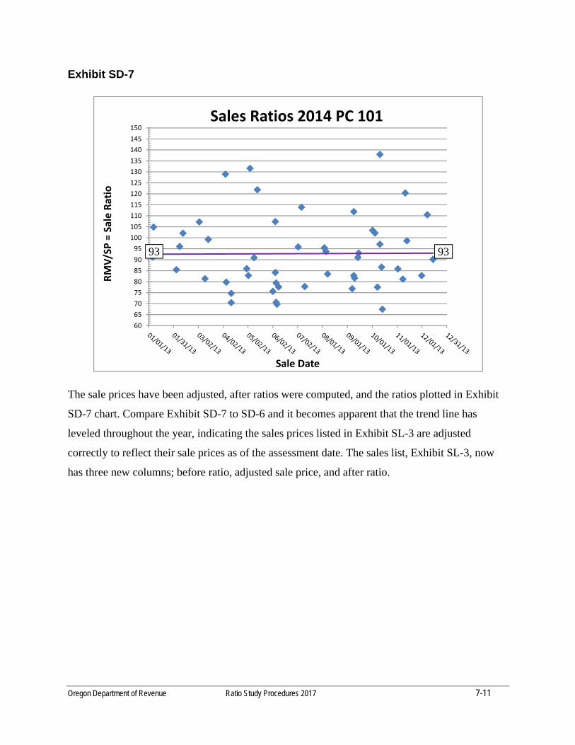
Oregon Department of Revenue Ratio Study Procedures 2017 7-11
Exhibit SD-7
The sale prices have been adjusted, after ratios were computed, and the ratios plotted in Exhibit
SD-7 chart. Compare Exhibit SD-7 to SD-6 and it becomes apparent that the trend line has
leveled throughout the year, indicating the sales prices listed in Exhibit SL-3 are adjusted
correctly to reflect their sale prices as of the assessment date. The sales list, Exhibit SL-3, now
has three new columns; before ratio, adjusted sale price, and after ratio.
60
65
70
75
80
85
90
95
100
105
110
115
120
125
130
135
140
145
150
RMV/SP = Sale Ratio
Sale Date
Sales Ratios 2014 PC 101
93 93
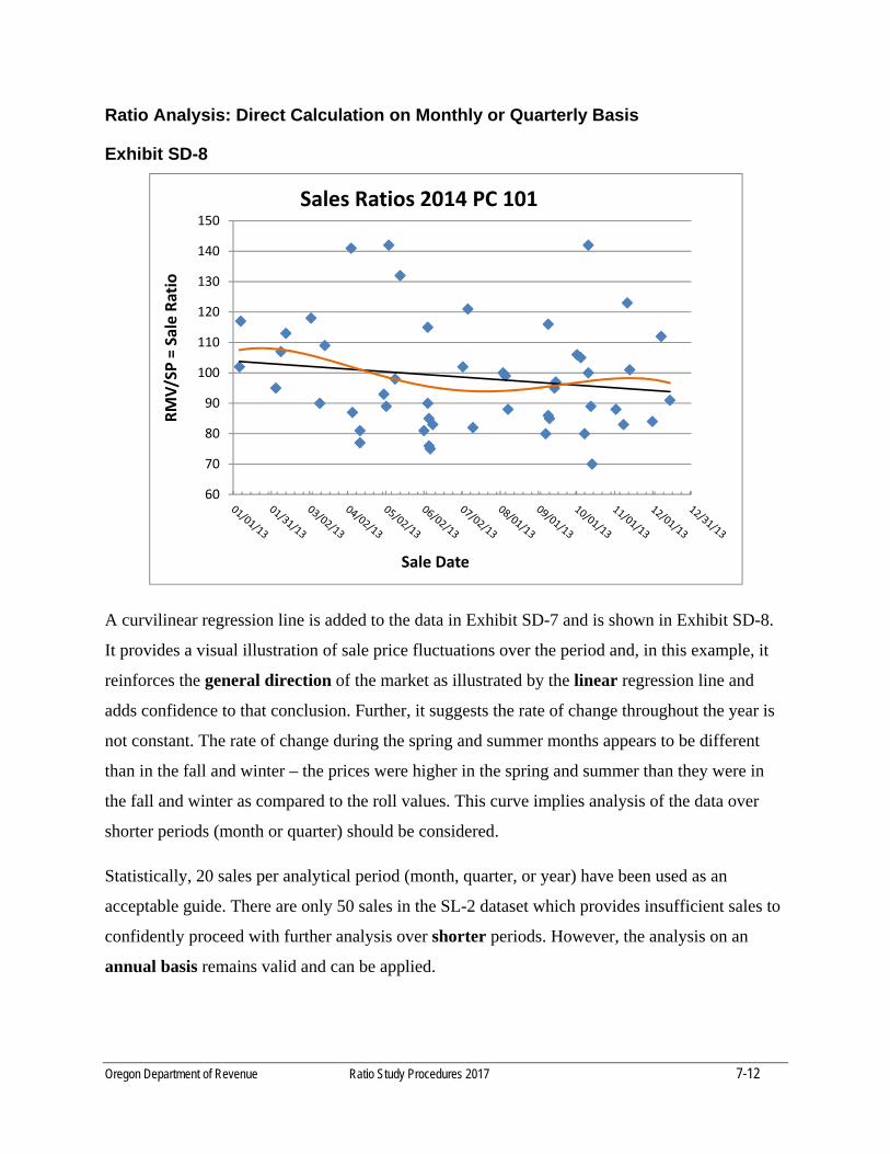
Oregon Department of Revenue Ratio Study Procedures 2017 7-12
Ratio Analysis: Direct Calculation on Monthly or Quarterly Basis
Exhibit SD-8
A curvilinear regression line is added to the data in Exhibit SD-7 and is shown in Exhibit SD-8.
It provides a visual illustration of sale price fluctuations over the period and, in this example, it
reinforces the general direction of the market as illustrated by the linear regression line and
adds confidence to that conclusion. Further, it suggests the rate of change throughout the year is
not constant. The rate of change during the spring and summer months appears to be different
than in the fall and winter – the prices were higher in the spring and summer than they were in
the fall and winter as compared to the roll values. This curve implies analysis of the data over
shorter periods (month or quarter) should be considered.
Statistically, 20 sales per analytical period (month, quarter, or year) have been used as an
acceptable guide. There are only 50 sales in the SL-2 dataset which provides insufficient sales to
confidently proceed with further analysis over shorter periods. However, the analysis on an
annual basis remains valid and can be applied.
60
70
80
90
100
110
120
130
140
150
RMV/SP = Sale Ratio
Sale Date
Sales Ratios 2014 PC 101

Oregon Department of Revenue Ratio Study Procedures 2017 7-13
Larger Datasets
A trimmed list of 505 sales (see Exhibit SL-4 at end of this section) contributes in excess of 20
sales per period providing a basis for sound statistical calculation of central tendencies for
shorter periods; in this example: month. Exhibit SD-9 plots the ratios of these sales with a linear
regression line applied that indicates the market increased over the year.
Exhibit SD-9
To analyze the sales over a shorter period (month and/or quarter):
1. Array the data in the sales list on a monthly and/or quarterly basis.
2. Confirm there are at least 20 sales per period.
3. Compute and table the central tendencies.
4. Select the central tendency that is most representative of the market for each period as
illustrated in Exhibit T-6.
The Selected Central Tendency is sometimes erroneously referred to as the Selected
Ratio. A ratio is a comparison between two numbers. A central tendency is a statistical
measure.
5. Include the table in the ratio study report.
0.50
0.60
0.70
0.80
0.90
1.00
1.10
1.20
1.30
1.40
1.50
RMV/SP = Sale Rato
PC 101 2014 Sales

Oregon Department of Revenue Ratio Study Procedures 2017 7-14
Exhibit T-6
Improved County Wide 101 Time Trend Analysis PC‐101 Ratio Table 2014 Sales
Month Month Count Cumulative
Count Median Mean W. Mean Selected
Jan 1 29 29 1.07 1.08 1.06 1.07
Feb 2 34 63 1.03 1.01 1.00 1.01
Mar 3 24 87 1.03 1.04 1.02 1.03
Apr 4 43 130 1.01 1.02 1.01 1.01
May 5 61 191 1.02 1.02 1.02 1.02
Jun 6 48 239 1.00 1.01 1.00 1.00
Jul 7 51 290 0.94 0.96 0.95 0.95
Aug 8 53 343 0.95 0.94 0.94 0.94
Sep 9 42 385 0.94 0.96 0.96 0.96
Oct 10 43 428 0.93 0.94 0.92 0.93
Nov 11 47 475 0.89 0.92 0.92 0.92
Dec 12 30 505 0.89 0.91 0.90 0.90
Total Sales:
505
Explanation of Central Tendency Selection
Month Selected Central Tendency Reason for Selection (data is not significantly skewed)
January Median Supported by the Mean and the Wtd. Mean
February Mean Bracketed by the Median and the Wtd. Mean
March Median Supported by the other central tendencies
April Median Supported by other central tendencies
May Median Same as the other central tendencies
June Median Supported by the Mean and the Wtd. Mean
July Weighted Mean Bracketed by the other central tendencies
August Mean Same as the Wtd. Mean; supported by the Median
September Mean Same as the Wtd. Mean; supported by the Median
October Median Bracketed by the Mean and the Wtd. Mean
November Weighted Mean Supported by the Mean
December Wtd. Mean Bracketed by the Mean and the Median
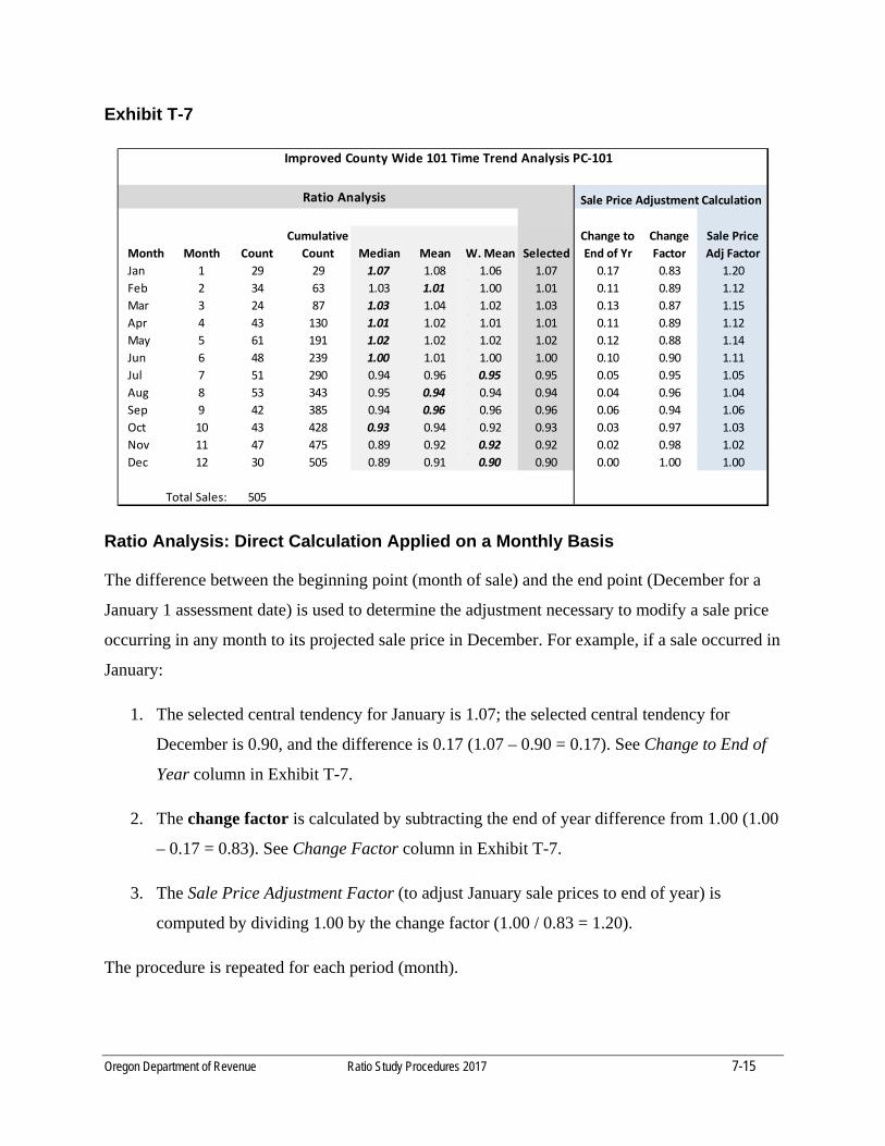
Oregon Department of Revenue Ratio Study Procedures 2017 7-15
Exhibit T-7
Ratio Analysis: Direct Calculation Applied on a Monthly Basis
The difference between the beginning point (month of sale) and the end point (December for a
January 1 assessment date) is used to determine the adjustment necessary to modify a sale price
occurring in any month to its projected sale price in December. For example, if a sale occurred in
January:
1. The selected central tendency for January is 1.07; the selected central tendency for
December is 0.90, and the difference is 0.17 (1.07 – 0.90 = 0.17). See Change to End of
Year column in Exhibit T-7.
2. The change factor is calculated by subtracting the end of year difference from 1.00 (1.00
– 0.17 = 0.83). See Change Factor column in Exhibit T-7.
3. The Sale Price Adjustment Factor (to adjust January sale prices to end of year) is
computed by dividing 1.00 by the change factor (1.00 / 0.83 = 1.20).
The procedure is repeated for each period (month).
Month Month Count
Cumulative
Count Median Mean W. Mean Selected
Change to
End of Yr
Change
Factor
Sale Price
Adj Factor
Jan 1 29 29 1.07 1.08 1.06 1.07 0.17 0.83 1.20
Feb 2 34 63 1.03 1.01 1.00 1.01 0.11 0.89 1.12
Mar 3 24 87 1.03 1.04 1.02 1.03 0.13 0.87 1.15
Apr 4 43 130 1.01 1.02 1.01 1.01 0.11 0.89 1.12
May 5 61 191 1.02 1.02 1.02 1.02 0.12 0.88 1.14
Jun 6 48 239 1.00 1.01 1.00 1.00 0.10 0.90 1.11
Jul 7 51 290 0.94 0.96 0.95 0.95 0.05 0.95 1.05
Aug 8 53 343 0.95 0.94 0.94 0.94 0.04 0.96 1.04
Sep 9 42 385 0.94 0.96 0.96 0.96 0.06 0.94 1.06
Oct 10 43 428 0.93 0.94 0.92 0.93 0.03 0.97 1.03
Nov 11 47 475 0.89 0.92 0.92 0.92 0.02 0.98 1.02
Dec 12 30 505 0.89 0.91 0.90 0.90 0.00 1.00 1.00
Total Sales: 505
Improved County Wide 101 Time Trend Analysis PC‐101
Ratio Analysis Sale Price Adjustment Calculation
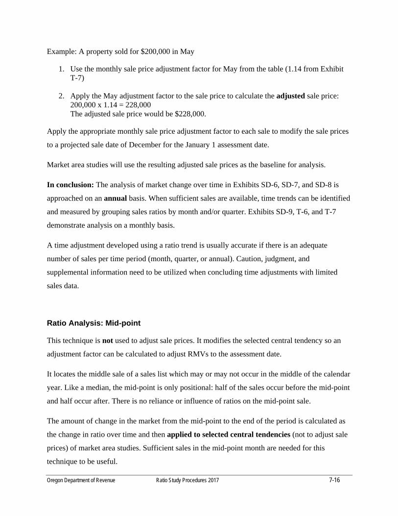
Oregon Department of Revenue Ratio Study Procedures 2017 7-16
Example: A property sold for $200,000 in May
1. Use the monthly sale price adjustment factor for May from the table (1.14 from Exhibit T-7)
2. Apply the May adjustment factor to the sale price to calculate the adjusted sale price:
200,000 x 1.14 = 228,000 The adjusted sale price would be $228,000.
Apply the appropriate monthly sale price adjustment factor to each sale to modify the sale prices
to a projected sale date of December for the January 1 assessment date.
Market area studies will use the resulting adjusted sale prices as the baseline for analysis.
In conclusion: The analysis of market change over time in Exhibits SD-6, SD-7, and SD-8 is
approached on an annual basis. When sufficient sales are available, time trends can be identified
and measured by grouping sales ratios by month and/or quarter. Exhibits SD-9, T-6, and T-7
demonstrate analysis on a monthly basis.
A time adjustment developed using a ratio trend is usually accurate if there is an adequate
number of sales per time period (month, quarter, or annual). Caution, judgment, and
supplemental information need to be utilized when concluding time adjustments with limited
sales data.
Ratio Analysis: Mid-point
This technique is not used to adjust sale prices. It modifies the selected central tendency so an
adjustment factor can be calculated to adjust RMVs to the assessment date.
It locates the middle sale of a sales list which may or may not occur in the middle of the calendar
year. Like a median, the mid-point is only positional: half of the sales occur before the mid-point
and half occur after. There is no reliance or influence of ratios on the mid-point sale.
The amount of change in the market from the mid-point to the end of the period is calculated as
the change in ratio over time and then applied to selected central tendencies (not to adjust sale
prices) of market area studies. Sufficient sales in the mid-point month are needed for this
technique to be useful.

Oregon Department of Revenue Ratio Study Procedures 2017 7-17
Step by step instructions to create a mid-point ratio table.
In the following table, a full year of sales is analyzed on a monthly basis.
1. Sort the sales in ascending order by the sale date.
2. Count the number of sales in each month and list in a
column in the table.
3. Next to the Month column from Step 2, calculate and
enter the cumulative sales count.
4. Total the number of sales in the entire sorted array.
5. Divide the total number of sales by 2 to locate middle sale, regardless of the month in
which it occurs.
(352 / 2 = 176)
6. Identify the month in the Cumulative Count column (created in Step 2) in which the
middle sale occurs.
(Sale number 176 falls in July so July is selected as the mid-point month.)
7. Compute the central tendencies for the mid-point month (July) and for December.
8. Select a central tendency that is the best fit for the mid-point month (July) and the end-
Cumulative
Month Month Count Count
Jan 1 18 18
Feb 2 16 34
Mar 3 11 45
Apr 4 29 74
May 5 30 104
Jun 6 38 142
Mid‐point Jul 7 43 185
Aug 8 32 217
Sep 9 41 258
Oct 10 39 297
Nov 11 32 329
Dec 12 23 352
Total Sales: 352
Cumulative
Month Month Count Count
Jan 1 18 18
Feb 2 16 34
Mar 3 11 45
Apr 4 29 74
May 5 30 104
Jun 6 38 142
Jul 7 43 185
Aug 8 32 217
Sep 9 41 258
Oct 10 39 297
Nov 11 32 329
Dec 12 23 352
Total Sales: 352
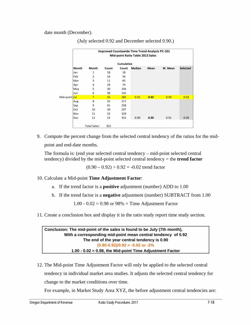
Oregon Department of Revenue Ratio Study Procedures 2017 7-18
date month (December).
(July selected 0.92 and December selected 0.90.)
9. Compute the percent change from the selected central tendency of the ratios for the mid-
point and end-date months.
The formula is: (end year selected central tendency – mid-point selected central tendency) divided by the mid-point selected central tendency = the trend factor
(0.90 – 0.92) ÷ 0.92 = -0.02 trend factor
10. Calculate a Mid-point Time Adjustment Factor:
a. If the trend factor is a positive adjustment (number) ADD to 1.00
b. If the trend factor is a negative adjustment (number) SUBTRACT from 1.00
1.00 - 0.02 = 0.98 or 98% = Time Adjustment Factor
11. Create a conclusion box and display it in the ratio study report time study section.
Conclusion: The mid-point of the sales is found to be July (7th month),
With a corresponding mid-point mean central tendency of 0.92 The end of the year central tendency is 0.90
(0.90-0.92)/0.92 = -0.02 or -2% 1.00 - 0.02 = 0.98, the Mid-point Time Adjustment Factor
12. The Mid-point Time Adjustment Factor will only be applied to the selected central
tendency in individual market area studies. It adjusts the selected central tendency for
change to the market conditions over time.
For example, in Market Study Area XYZ, the before adjustment central tendencies are:
Cumulative
Month Month Count Count Median Mean W. Mean Selected
Jan 1 18 18
Feb 2 16 34
Mar 3 11 45
Apr 4 29 74
May 5 30 104
Jun 6 38 142
Mid‐point Jul 7 43 185 0.91 0.92 0.93 0.92
Aug 8 32 217
Sep 9 41 258
Oct 10 39 297
Nov 11 32 329
Dec 12 23 352 0.90 0.90 0.91 0.90
Total Sales: 352
Improved Countywide Time Trend Analysis PC‐101Mid‐point Ratio Table 2013 Sales
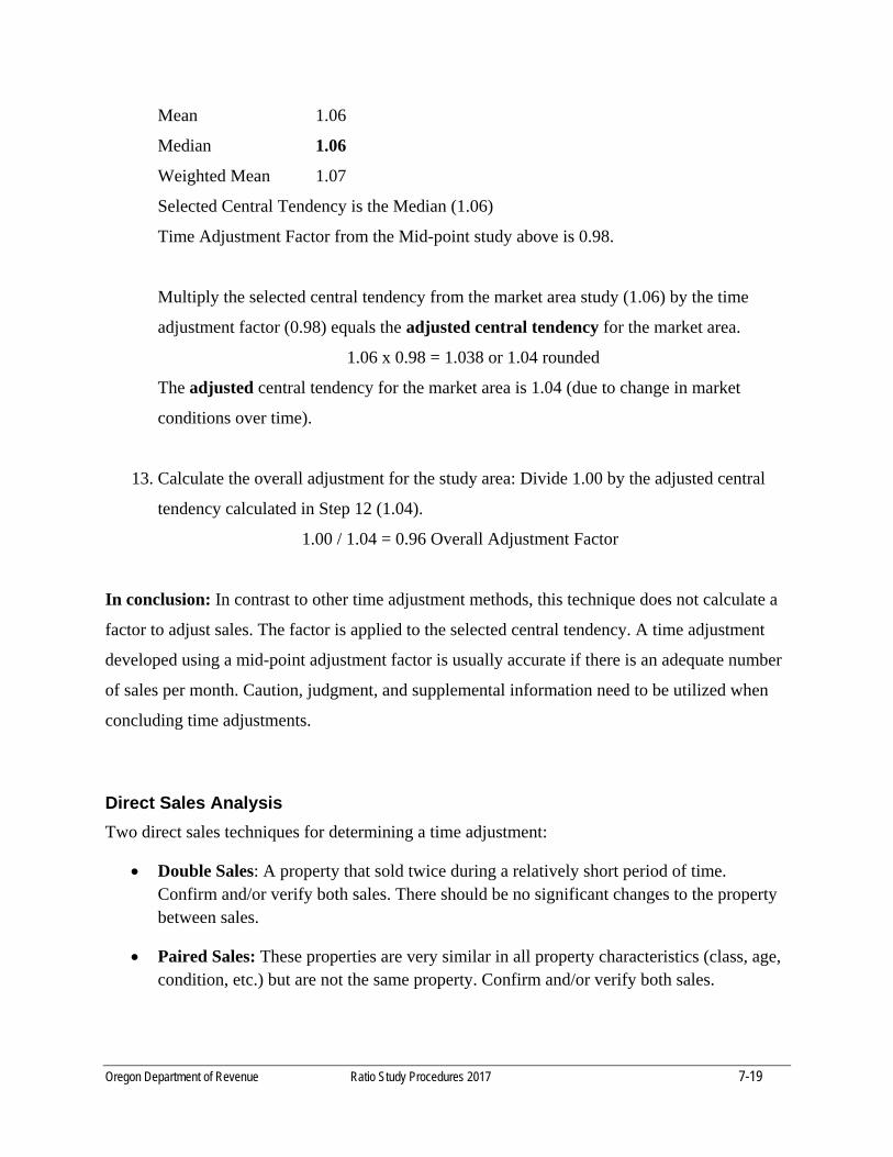
Oregon Department of Revenue Ratio Study Procedures 2017 7-19
Mean 1.06
Median 1.06
Weighted Mean 1.07
Selected Central Tendency is the Median (1.06)
Time Adjustment Factor from the Mid-point study above is 0.98.
Multiply the selected central tendency from the market area study (1.06) by the time
adjustment factor (0.98) equals the adjusted central tendency for the market area.
1.06 x 0.98 = 1.038 or 1.04 rounded
The adjusted central tendency for the market area is 1.04 (due to change in market
conditions over time).
13. Calculate the overall adjustment for the study area: Divide 1.00 by the adjusted central
tendency calculated in Step 12 (1.04).
1.00 / 1.04 = 0.96 Overall Adjustment Factor
In conclusion: In contrast to other time adjustment methods, this technique does not calculate a
factor to adjust sales. The factor is applied to the selected central tendency. A time adjustment
developed using a mid-point adjustment factor is usually accurate if there is an adequate number
of sales per month. Caution, judgment, and supplemental information need to be utilized when
concluding time adjustments.
Direct Sales Analysis
Two direct sales techniques for determining a time adjustment:
Double Sales: A property that sold twice during a relatively short period of time. Confirm and/or verify both sales. There should be no significant changes to the property between sales.
Paired Sales: These properties are very similar in all property characteristics (class, age, condition, etc.) but are not the same property. Confirm and/or verify both sales.
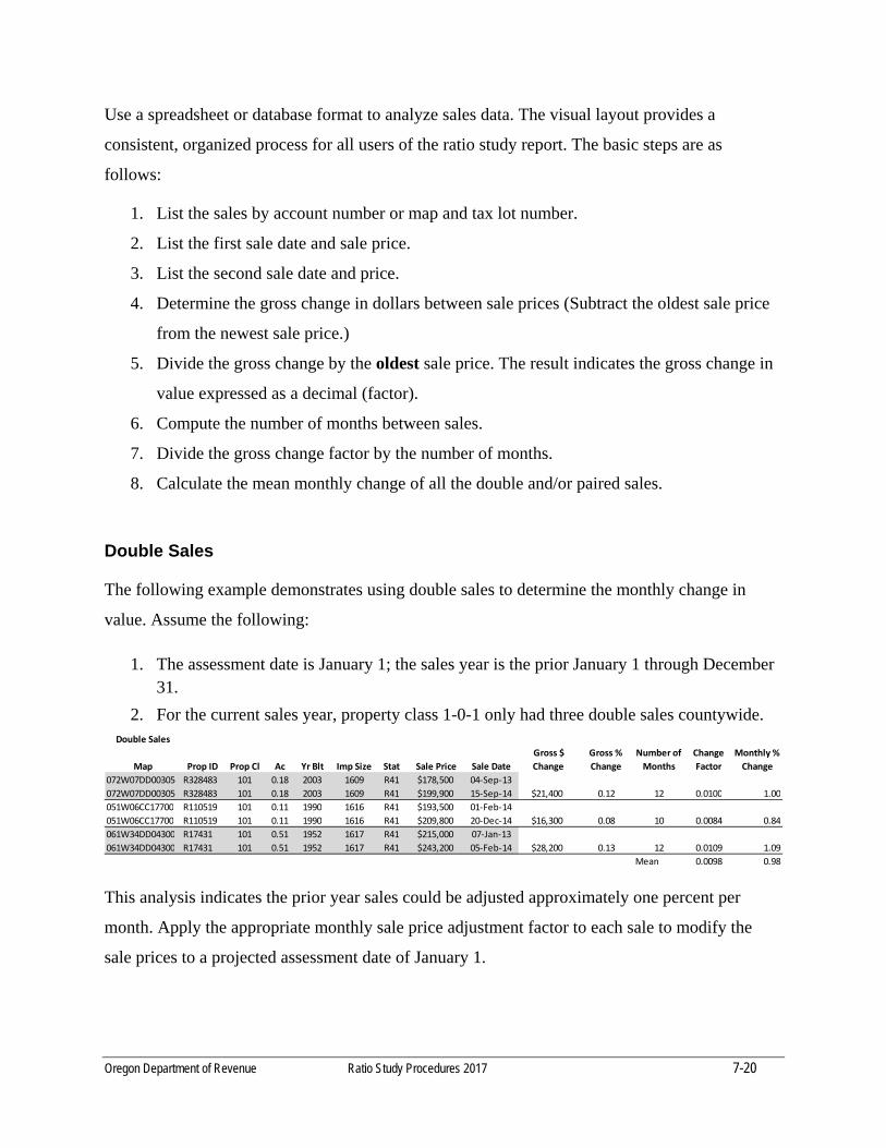
Oregon Department of Revenue Ratio Study Procedures 2017 7-20
Use a spreadsheet or database format to analyze sales data. The visual layout provides a
consistent, organized process for all users of the ratio study report. The basic steps are as
follows:
1. List the sales by account number or map and tax lot number.
2. List the first sale date and sale price.
3. List the second sale date and price.
4. Determine the gross change in dollars between sale prices (Subtract the oldest sale price
from the newest sale price.)
5. Divide the gross change by the oldest sale price. The result indicates the gross change in
value expressed as a decimal (factor).
6. Compute the number of months between sales.
7. Divide the gross change factor by the number of months.
8. Calculate the mean monthly change of all the double and/or paired sales.
Double Sales
The following example demonstrates using double sales to determine the monthly change in
value. Assume the following:
1. The assessment date is January 1; the sales year is the prior January 1 through December 31.
2. For the current sales year, property class 1-0-1 only had three double sales countywide.
This analysis indicates the prior year sales could be adjusted approximately one percent per
month. Apply the appropriate monthly sale price adjustment factor to each sale to modify the
sale prices to a projected assessment date of January 1.
Double Sales
Map Prop ID Prop Cl Ac Yr Blt Imp Size Stat Sale Price Sale Date
Gross $
Change
Gross %
Change
Number of
Months
Change
Factor
Monthly %
Change
072W07DD00305 R328483 101 0.18 2003 1609 R41 $178,500 04‐Sep‐13
072W07DD00305 R328483 101 0.18 2003 1609 R41 $199,900 15‐Sep‐14 $21,400 0.12 12 0.0100 1.00
051W06CC17700 R110519 101 0.11 1990 1616 R41 $193,500 01‐Feb‐14
051W06CC17700 R110519 101 0.11 1990 1616 R41 $209,800 20‐Dec‐14 $16,300 0.08 10 0.0084 0.84
061W34DD04300 R17431 101 0.51 1952 1617 R41 $215,000 07‐Jan‐13
061W34DD04300 R17431 101 0.51 1952 1617 R41 $243,200 05‐Feb‐14 $28,200 0.13 12 0.0109 1.09
Mean 0.0098 0.98
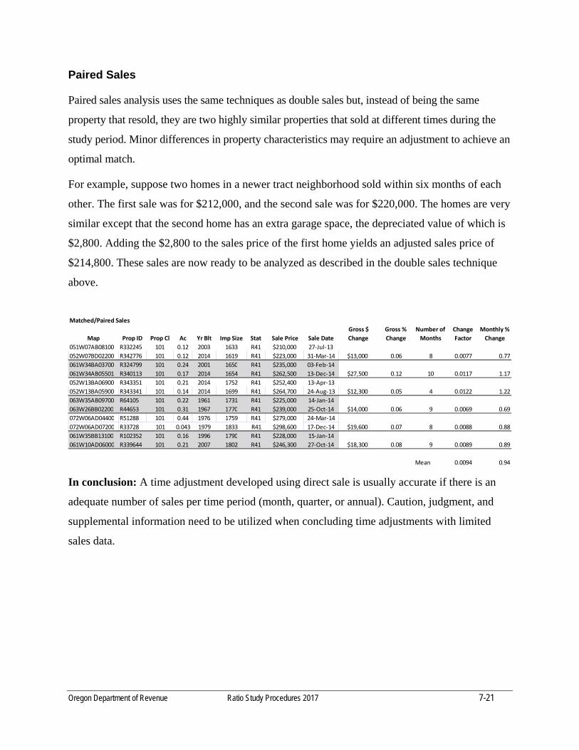
Oregon Department of Revenue Ratio Study Procedures 2017 7-21
Paired Sales
Paired sales analysis uses the same techniques as double sales but, instead of being the same
property that resold, they are two highly similar properties that sold at different times during the
study period. Minor differences in property characteristics may require an adjustment to achieve an
optimal match.
For example, suppose two homes in a newer tract neighborhood sold within six months of each
other. The first sale was for $212,000, and the second sale was for $220,000. The homes are very
similar except that the second home has an extra garage space, the depreciated value of which is
$2,800. Adding the $2,800 to the sales price of the first home yields an adjusted sales price of
$214,800. These sales are now ready to be analyzed as described in the double sales technique
above.
In conclusion: A time adjustment developed using direct sale is usually accurate if there is an
adequate number of sales per time period (month, quarter, or annual). Caution, judgment, and
supplemental information need to be utilized when concluding time adjustments with limited
sales data.
Map Prop ID Prop Cl Ac Yr Blt Imp Size Stat Sale Price Sale Date
Gross $
Change
Gross %
Change
Number of
Months
Change
Factor
Monthly %
Change
051W07AB08100 R332245 101 0.12 2003 1633 R41 $210,000 27‐Jul‐13
052W07BD02200 R342776 101 0.12 2014 1619 R41 $223,000 31‐Mar‐14 $13,000 0.06 8 0.0077 0.77
061W34BA03700 R324799 101 0.24 2001 1650 R41 $235,000 03‐Feb‐14
061W34AB05501 R340113 101 0.17 2014 1654 R41 $262,500 13‐Dec‐14 $27,500 0.12 10 0.0117 1.17
052W13BA06900 R343351 101 0.21 2014 1752 R41 $252,400 13‐Apr‐13
052W13BA05900 R343341 101 0.14 2014 1699 R41 $264,700 24‐Aug‐13 $12,300 0.05 4 0.0122 1.22
063W35AB09700 R64105 101 0.22 1961 1731 R41 $225,000 14‐Jan‐14
063W26BB02200 R44653 101 0.31 1967 1770 R41 $239,000 25‐Oct‐14 $14,000 0.06 9 0.0069 0.69
072W06AD04400 R51288 101 0.44 1976 1759 R41 $279,000 24‐Mar‐14
072W06AD07200 R33728 101 0.043 1979 1833 R41 $298,600 17‐Dec‐14 $19,600 0.07 8 0.0088 0.88
061W35BB13100 R102352 101 0.16 1996 1790 R41 $228,000 15‐Jan‐14
061W10AD06000 R339644 101 0.21 2007 1802 R41 $246,300 27‐Oct‐14 $18,300 0.08 9 0.0089 0.89
Mean 0.0094 0.94
Matched/Paired Sales

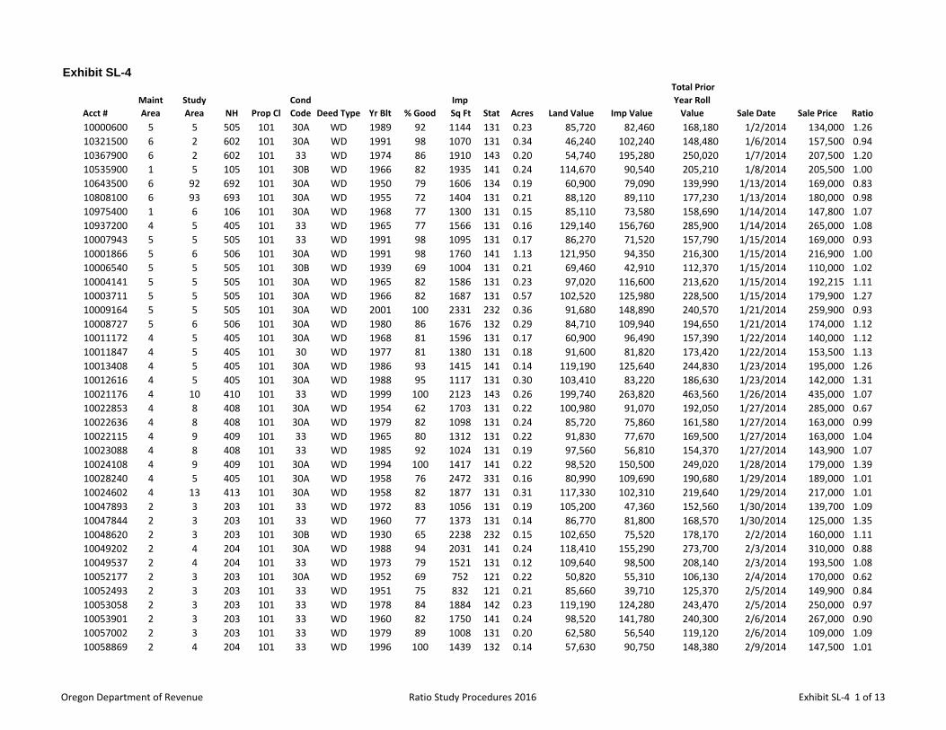
Exhibit SL-4
Acct #
Maint
Area
Study
Area NH Prop Cl
Cond
Code Deed Type Yr Blt % Good
Imp
Sq Ft Stat Acres Land Value Imp Value
Total Prior
Year Roll
Value Sale Date Sale Price Ratio
10000600 5 5 505 101 30A WD 1989 92 1144 131 0.23 85,720 82,460 168,180 1/2/2014 134,000 1.26
10321500 6 2 602 101 30A WD 1991 98 1070 131 0.34 46,240 102,240 148,480 1/6/2014 157,500 0.94
10367900 6 2 602 101 33 WD 1974 86 1910 143 0.20 54,740 195,280 250,020 1/7/2014 207,500 1.20
10535900 1 5 105 101 30B WD 1966 82 1935 141 0.24 114,670 90,540 205,210 1/8/2014 205,500 1.00
10643500 6 92 692 101 30A WD 1950 79 1606 134 0.19 60,900 79,090 139,990 1/13/2014 169,000 0.83
10808100 6 93 693 101 30A WD 1955 72 1404 131 0.21 88,120 89,110 177,230 1/13/2014 180,000 0.98
10975400 1 6 106 101 30A WD 1968 77 1300 131 0.15 85,110 73,580 158,690 1/14/2014 147,800 1.07
10937200 4 5 405 101 33 WD 1965 77 1566 131 0.16 129,140 156,760 285,900 1/14/2014 265,000 1.08
10007943 5 5 505 101 33 WD 1991 98 1095 131 0.17 86,270 71,520 157,790 1/15/2014 169,000 0.93
10001866 5 6 506 101 30A WD 1991 98 1760 141 1.13 121,950 94,350 216,300 1/15/2014 216,900 1.00
10006540 5 5 505 101 30B WD 1939 69 1004 131 0.21 69,460 42,910 112,370 1/15/2014 110,000 1.02
10004141 5 5 505 101 30A WD 1965 82 1586 131 0.23 97,020 116,600 213,620 1/15/2014 192,215 1.11
10003711 5 5 505 101 30A WD 1966 82 1687 131 0.57 102,520 125,980 228,500 1/15/2014 179,900 1.27
10009164 5 5 505 101 30A WD 2001 100 2331 232 0.36 91,680 148,890 240,570 1/21/2014 259,900 0.93
10008727 5 6 506 101 30A WD 1980 86 1676 132 0.29 84,710 109,940 194,650 1/21/2014 174,000 1.12
10011172 4 5 405 101 30A WD 1968 81 1596 131 0.17 60,900 96,490 157,390 1/22/2014 140,000 1.12
10011847 4 5 405 101 30 WD 1977 81 1380 131 0.18 91,600 81,820 173,420 1/22/2014 153,500 1.13
10013408 4 5 405 101 30A WD 1986 93 1415 141 0.14 119,190 125,640 244,830 1/23/2014 195,000 1.26
10012616 4 5 405 101 30A WD 1988 95 1117 131 0.30 103,410 83,220 186,630 1/23/2014 142,000 1.31
10021176 4 10 410 101 33 WD 1999 100 2123 143 0.26 199,740 263,820 463,560 1/26/2014 435,000 1.07
10022853 4 8 408 101 30A WD 1954 62 1703 131 0.22 100,980 91,070 192,050 1/27/2014 285,000 0.67
10022636 4 8 408 101 30A WD 1979 82 1098 131 0.24 85,720 75,860 161,580 1/27/2014 163,000 0.99
10022115 4 9 409 101 33 WD 1965 80 1312 131 0.22 91,830 77,670 169,500 1/27/2014 163,000 1.04
10023088 4 8 408 101 33 WD 1985 92 1024 131 0.19 97,560 56,810 154,370 1/27/2014 143,900 1.07
10024108 4 9 409 101 30A WD 1994 100 1417 141 0.22 98,520 150,500 249,020 1/28/2014 179,000 1.39
10028240 4 5 405 101 30A WD 1958 76 2472 331 0.16 80,990 109,690 190,680 1/29/2014 189,000 1.01
10024602 4 13 413 101 30A WD 1958 82 1877 131 0.31 117,330 102,310 219,640 1/29/2014 217,000 1.01
10047893 2 3 203 101 33 WD 1972 83 1056 131 0.19 105,200 47,360 152,560 1/30/2014 139,700 1.09
10047844 2 3 203 101 33 WD 1960 77 1373 131 0.14 86,770 81,800 168,570 1/30/2014 125,000 1.35
10048620 2 3 203 101 30B WD 1930 65 2238 232 0.15 102,650 75,520 178,170 2/2/2014 160,000 1.11
10049202 2 4 204 101 30A WD 1988 94 2031 141 0.24 118,410 155,290 273,700 2/3/2014 310,000 0.88
10049537 2 4 204 101 33 WD 1973 79 1521 131 0.12 109,640 98,500 208,140 2/3/2014 193,500 1.08
10052177 2 3 203 101 30A WD 1952 69 752 121 0.22 50,820 55,310 106,130 2/4/2014 170,000 0.62
10052493 2 3 203 101 33 WD 1951 75 832 121 0.21 85,660 39,710 125,370 2/5/2014 149,900 0.84
10053058 2 3 203 101 33 WD 1978 84 1884 142 0.23 119,190 124,280 243,470 2/5/2014 250,000 0.97
10053901 2 3 203 101 33 WD 1960 82 1750 141 0.24 98,520 141,780 240,300 2/6/2014 267,000 0.90
10057002 2 3 203 101 33 WD 1979 89 1008 131 0.20 62,580 56,540 119,120 2/6/2014 109,000 1.09
10058869 2 4 204 101 33 WD 1996 100 1439 132 0.14 57,630 90,750 148,380 2/9/2014 147,500 1.01
Oregon Department of Revenue Ratio Study Procedures 2016 Exhibit SL‐4 1 of 13
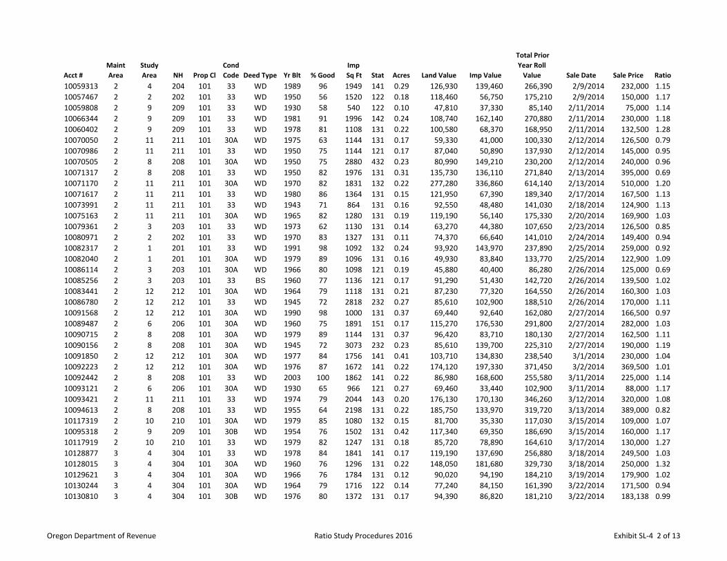
Acct #
Maint
Area
Study
Area NH Prop Cl
Cond
Code Deed Type Yr Blt % Good
Imp
Sq Ft Stat Acres Land Value Imp Value
Total Prior
Year Roll
Value Sale Date Sale Price Ratio
10059313 2 4 204 101 33 WD 1989 96 1949 141 0.29 126,930 139,460 266,390 2/9/2014 232,000 1.15
10057467 2 2 202 101 33 WD 1950 56 1520 122 0.18 118,460 56,750 175,210 2/9/2014 150,000 1.17
10059808 2 9 209 101 33 WD 1930 58 540 122 0.10 47,810 37,330 85,140 2/11/2014 75,000 1.14
10066344 2 9 209 101 33 WD 1981 91 1996 142 0.24 108,740 162,140 270,880 2/11/2014 230,000 1.18
10060402 2 9 209 101 33 WD 1978 81 1108 131 0.22 100,580 68,370 168,950 2/11/2014 132,500 1.28
10070050 2 11 211 101 30A WD 1975 63 1144 131 0.17 59,330 41,000 100,330 2/12/2014 126,500 0.79
10070986 2 11 211 101 33 WD 1950 75 1144 121 0.17 87,040 50,890 137,930 2/12/2014 145,000 0.95
10070505 2 8 208 101 30A WD 1950 75 2880 432 0.23 80,990 149,210 230,200 2/12/2014 240,000 0.96
10071317 2 8 208 101 33 WD 1950 82 1976 131 0.31 135,730 136,110 271,840 2/13/2014 395,000 0.69
10071170 2 11 211 101 30A WD 1970 82 1831 132 0.22 277,280 336,860 614,140 2/13/2014 510,000 1.20
10071617 2 11 211 101 33 WD 1980 86 1364 131 0.15 121,950 67,390 189,340 2/17/2014 167,500 1.13
10073991 2 11 211 101 33 WD 1943 71 864 131 0.16 92,550 48,480 141,030 2/18/2014 124,900 1.13
10075163 2 11 211 101 30A WD 1965 82 1280 131 0.19 119,190 56,140 175,330 2/20/2014 169,900 1.03
10079361 2 3 203 101 33 WD 1973 62 1130 131 0.14 63,270 44,380 107,650 2/23/2014 126,500 0.85
10080971 2 2 202 101 33 WD 1970 83 1327 131 0.11 74,370 66,640 141,010 2/24/2014 149,400 0.94
10082317 2 1 201 101 33 WD 1991 98 1092 132 0.24 93,920 143,970 237,890 2/25/2014 259,000 0.92
10082040 2 1 201 101 30A WD 1979 89 1096 131 0.16 49,930 83,840 133,770 2/25/2014 122,900 1.09
10086114 2 3 203 101 30A WD 1966 80 1098 121 0.19 45,880 40,400 86,280 2/26/2014 125,000 0.69
10085256 2 3 203 101 33 BS 1960 77 1136 121 0.17 91,290 51,430 142,720 2/26/2014 139,500 1.02
10083441 2 12 212 101 30A WD 1964 79 1118 131 0.21 87,230 77,320 164,550 2/26/2014 160,300 1.03
10086780 2 12 212 101 33 WD 1945 72 2818 232 0.27 85,610 102,900 188,510 2/26/2014 170,000 1.11
10091568 2 12 212 101 30A WD 1990 98 1000 131 0.37 69,440 92,640 162,080 2/27/2014 166,500 0.97
10089487 2 6 206 101 30A WD 1960 75 1891 151 0.17 115,270 176,530 291,800 2/27/2014 282,000 1.03
10090715 2 8 208 101 30A WD 1979 89 1144 131 0.37 96,420 83,710 180,130 2/27/2014 162,500 1.11
10090156 2 8 208 101 30A WD 1945 72 3073 232 0.23 85,610 139,700 225,310 2/27/2014 190,000 1.19
10091850 2 12 212 101 30A WD 1977 84 1756 141 0.41 103,710 134,830 238,540 3/1/2014 230,000 1.04
10092223 2 12 212 101 30A WD 1976 87 1672 141 0.22 174,120 197,330 371,450 3/2/2014 369,500 1.01
10092442 2 8 208 101 33 WD 2003 100 1862 141 0.22 86,980 168,600 255,580 3/11/2014 225,000 1.14
10093121 2 6 206 101 30A WD 1930 65 966 121 0.27 69,460 33,440 102,900 3/11/2014 88,000 1.17
10093421 2 11 211 101 33 WD 1974 79 2044 143 0.20 176,130 170,130 346,260 3/12/2014 320,000 1.08
10094613 2 8 208 101 33 WD 1955 64 2198 131 0.22 185,750 133,970 319,720 3/13/2014 389,000 0.82
10117319 2 10 210 101 30A WD 1979 85 1080 132 0.15 81,700 35,330 117,030 3/15/2014 109,000 1.07
10095318 2 9 209 101 30B WD 1954 76 1502 131 0.42 117,340 69,350 186,690 3/15/2014 160,000 1.17
10117919 2 10 210 101 33 WD 1979 82 1247 131 0.18 85,720 78,890 164,610 3/17/2014 130,000 1.27
10128877 3 4 304 101 33 WD 1978 84 1841 141 0.17 119,190 137,690 256,880 3/18/2014 249,500 1.03
10128015 3 4 304 101 30A WD 1960 76 1296 131 0.22 148,050 181,680 329,730 3/18/2014 250,000 1.32
10129621 3 4 304 101 30A WD 1966 76 1784 131 0.12 90,020 94,190 184,210 3/19/2014 179,900 1.02
10130244 3 4 304 101 30A WD 1964 79 1716 122 0.14 77,240 84,150 161,390 3/22/2014 171,500 0.94
10130810 3 4 304 101 30B WD 1976 80 1372 131 0.17 94,390 86,820 181,210 3/22/2014 183,138 0.99
Oregon Department of Revenue Ratio Study Procedures 2016 Exhibit SL‐4 2 of 13
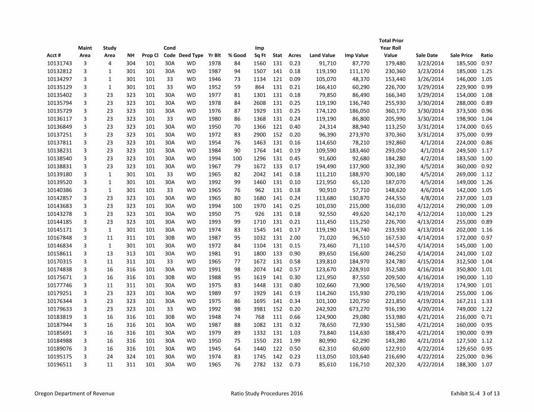
Acct #
Maint
Area
Study
Area NH Prop Cl
Cond
Code Deed Type Yr Blt % Good
Imp
Sq Ft Stat Acres Land Value Imp Value
Total Prior
Year Roll
Value Sale Date Sale Price Ratio
10131743 3 4 304 101 30A WD 1978 84 1560 131 0.23 91,710 87,770 179,480 3/23/2014 185,500 0.97
10132812 3 1 301 101 30A WD 1987 94 1507 141 0.18 119,190 111,170 230,360 3/23/2014 185,000 1.25
10134297 3 1 301 101 33 WD 1946 73 1134 121 0.09 105,070 48,370 153,440 3/26/2014 146,000 1.05
10135129 3 1 301 101 33 WD 1952 59 864 131 0.21 166,410 60,290 226,700 3/29/2014 229,900 0.99
10135402 3 23 323 101 30A WD 1977 81 1301 131 0.18 79,850 86,490 166,340 3/29/2014 154,000 1.08
10135794 3 23 323 101 30A WD 1978 84 2608 131 0.25 119,190 136,740 255,930 3/30/2014 288,000 0.89
10135729 3 23 323 101 30A WD 1976 87 1929 131 0.25 174,120 186,050 360,170 3/30/2014 373,500 0.96
10136117 3 23 323 101 33 WD 1980 86 1368 131 0.24 119,190 86,800 205,990 3/30/2014 198,900 1.04
10136849 3 23 323 101 30A WD 1950 70 1366 121 0.40 24,314 88,940 113,250 3/31/2014 174,000 0.65
10137251 3 23 323 101 30A WD 1972 83 2900 152 0.20 96,390 273,970 370,360 3/31/2014 375,000 0.99
10137811 3 23 323 101 30A WD 1954 76 1463 131 0.16 114,650 78,210 192,860 4/1/2014 224,000 0.86
10138231 3 23 323 101 30A WD 1984 90 1764 141 0.19 109,590 183,460 293,050 4/1/2014 249,500 1.17
10138540 3 23 323 101 30A WD 1994 100 1296 131 0.45 91,600 92,680 184,280 4/2/2014 183,500 1.00
10138831 3 23 323 101 30A WD 1967 79 1672 133 0.17 194,490 137,900 332,390 4/5/2014 360,000 0.92
10139180 3 1 301 101 33 WD 1965 82 2042 141 0.18 111,210 188,970 300,180 4/5/2014 269,000 1.12
10139520 3 1 301 101 30A WD 1992 99 1460 131 0.10 121,950 65,120 187,070 4/5/2014 149,000 1.26
10140386 3 1 301 101 33 WD 1965 76 962 131 0.18 90,910 57,710 148,620 4/6/2014 142,000 1.05
10142857 3 23 323 101 30A WD 1965 80 1680 141 0.24 113,680 130,870 244,550 4/8/2014 237,000 1.03
10143683 3 23 323 101 30A WD 1994 100 1970 141 0.25 101,030 215,000 316,030 4/12/2014 290,000 1.09
10143278 3 23 323 101 30A WD 1950 75 926 131 0.18 92,550 49,620 142,170 4/12/2014 110,000 1.29
10144185 3 23 323 101 30A WD 1993 99 1710 131 0.21 111,450 115,250 226,700 4/13/2014 255,000 0.89
10145171 3 1 301 101 30A WD 1974 83 1545 141 0.17 119,190 114,740 233,930 4/13/2014 202,000 1.16
10167848 3 11 311 101 30B WD 1987 95 1032 131 2.00 71,020 96,510 167,530 4/14/2014 172,000 0.97
10146834 3 1 301 101 30A WD 1972 84 1104 131 0.15 73,460 71,110 144,570 4/14/2014 145,000 1.00
10158611 3 13 313 101 30A WD 1981 91 1800 133 0.90 89,650 156,600 246,250 4/14/2014 241,000 1.02
10170315 3 11 311 101 33 WD 1965 77 1672 131 0.58 139,810 184,970 324,780 4/15/2014 312,500 1.04
10174838 3 16 316 101 30A WD 1991 98 2074 142 0.57 123,670 228,910 352,580 4/16/2014 350,800 1.01
10175671 3 16 316 101 30B WD 1988 95 1619 141 0.30 121,950 87,550 209,500 4/16/2014 190,000 1.10
10177746 3 11 311 101 30A WD 1975 83 1448 131 0.80 102,660 73,900 176,560 4/19/2014 174,900 1.01
10179251 3 23 323 101 30A WD 1989 97 1929 141 0.19 114,260 155,930 270,190 4/19/2014 255,000 1.06
10176344 3 23 323 101 30A WD 1975 86 1695 141 0.34 101,100 120,750 221,850 4/19/2014 167,211 1.33
10179633 3 23 323 101 33 WD 1992 98 3981 152 0.20 242,920 673,270 916,190 4/20/2014 749,000 1.22
10183819 3 16 316 101 30B WD 1948 74 768 111 0.66 124,900 29,080 153,980 4/21/2014 216,000 0.71
10187944 3 16 316 101 30A WD 1987 88 1082 131 0.32 78,650 72,930 151,580 4/21/2014 160,000 0.95
10185691 3 16 316 101 30A WD 1979 89 1332 131 1.03 73,840 114,630 188,470 4/21/2014 190,000 0.99
10184988 3 16 316 101 30A WD 1950 75 1550 231 1.99 80,990 62,290 143,280 4/21/2014 127,500 1.12
10189076 3 16 316 101 30A WD 1945 64 1440 122 0.50 62,310 60,600 122,910 4/22/2014 129,650 0.95
10195175 3 24 324 101 30A WD 1974 83 1745 142 0.23 113,050 103,640 216,690 4/22/2014 225,000 0.96
10196511 3 11 311 101 30A WD 1965 76 2782 132 0.73 85,610 116,710 202,320 4/22/2014 188,300 1.07
Oregon Department of Revenue Ratio Study Procedures 2016 Exhibit SL‐4 3 of 13
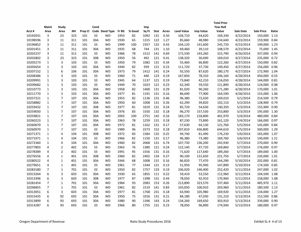
Acct #
Maint
Area
Study
Area NH Prop Cl
Cond
Code Deed Type Yr Blt % Good
Imp
Sq Ft Stat Acres Land Value Imp Value
Total Prior
Year Roll
Value Sale Date Sale Price Ratio
10192031 3 23 323 101 33 WD 1953 82 1092 131 0.50 104,710 64,620 169,330 4/22/2014 150,000 1.13
10198596 3 11 311 101 30A WD 1930 65 1315 122 1.27 85,660 48,980 134,640 4/23/2014 159,900 0.84
10196852 3 11 311 101 33 WD 1999 100 2357 132 0.43 104,120 141,600 245,720 4/23/2014 199,000 1.23
10201451 3 11 311 101 30A WD 1935 68 744 131 1.10 69,460 39,110 108,570 4/23/2014 75,000 1.45
10202237 3 11 311 101 33 WD 1966 78 1512 141 0.69 172,530 143,260 315,790 4/26/2014 337,000 0.94
10202802 3 23 323 101 30B WD 1950 56 492 121 0.41 138,320 30,690 169,010 4/27/2014 235,000 0.72
10205273 1 3 103 101 33 WD 1950 79 1082 131 0.34 55,460 66,800 122,260 4/27/2014 150,000 0.82
10205654 1 3 103 101 30A WD 1940 82 939 121 0.23 111,720 37,730 149,450 4/27/2014 156,000 0.96
10207152 1 6 106 101 30A WD 1973 79 1412 141 0.24 92,550 87,620 180,170 4/27/2014 172,900 1.04
10208386 1 3 103 101 33 WD 1960 71 440 123 0.19 167,850 78,310 246,160 4/28/2014 450,000 0.55
10209991 1 3 103 101 33 WD 1945 64 1137 121 0.19 73,840 42,210 116,050 4/28/2014 144,000 0.81
10209682 1 3 103 101 33 WD 1949 70 1023 121 0.23 62,340 59,550 121,890 4/28/2014 124,000 0.98
10210773 1 3 103 101 30A WD 1958 82 1400 131 0.29 81,020 90,260 171,280 4/28/2014 170,000 1.01
10211770 1 3 103 101 30A WD 1977 81 1191 131 0.16 86,690 77,900 164,590 4/28/2014 155,000 1.06
10257221 1 7 107 101 30A WD 1953 82 1136 131 0.46 96,380 72,630 169,010 5/1/2014 214,500 0.79
10258882 1 7 107 101 30A WD 1950 60 1008 131 0.26 62,290 39,820 102,110 5/2/2014 128,900 0.79
10259432 1 7 107 101 30B WD 1977 81 1019 131 0.24 85,720 54,630 140,350 5/3/2014 155,900 0.90
10259050 1 7 107 101 30A WD 1976 83 1550 132 0.18 96,270 157,530 253,800 5/3/2014 195,000 1.30
10259821 1 7 107 101 30A WD 2003 100 2751 142 0.16 183,170 218,800 401,970 5/4/2014 480,000 0.84
10260223 1 7 107 101 30A WD 1963 78 1259 131 0.18 87,230 73,890 161,120 5/4/2014 166,000 0.97
10260670 1 7 107 101 30A WD 1972 81 1162 131 0.17 57,630 64,130 121,760 5/5/2014 145,000 0.84
10260970 1 7 107 101 33 WD 1989 96 2273 152 0.18 207,810 436,800 644,610 5/5/2014 500,000 1.29
10271371 1 4 104 101 30B WD 1972 83 1584 132 0.25 94,740 81,490 176,230 5/6/2014 165,000 1.07
10271971 1 4 104 101 33 WD 1966 82 1150 131 0.17 96,380 73,380 169,760 5/6/2014 140,000 1.21
10272360 1 4 104 101 30A WD 1960 82 2068 131 6.74 107,730 136,200 243,930 5/7/2014 270,000 0.90
10277803 4 2 402 101 33 WD 1963 76 1380 121 0.24 122,140 47,720 169,860 5/7/2014 176,000 0.97
10278389 4 2 402 101 33 WD 1991 95 1556 131 0.16 71,620 117,640 189,260 5/7/2014 189,000 1.00
10276556 4 1 401 101 30B WD 1960 82 2402 134 0.27 90,100 131,650 221,750 5/7/2014 220,000 1.01
10280522 4 1 401 101 30A WD 1946 68 1008 131 0.16 86,820 77,470 164,290 5/10/2014 202,000 0.81
10279651 4 1 401 101 33 WD 1961 77 1344 121 0.13 51,950 95,940 147,890 5/10/2014 174,500 0.85
10283180 7 1 701 101 33 WD 1950 82 1757 133 0.19 106,020 146,400 252,420 5/11/2014 247,000 1.02
10313264 6 3 603 101 30A WD 1930 65 1855 111 0.22 59,410 53,550 112,960 5/11/2014 104,500 1.08
10313396 6 3 603 101 30B WD 1977 87 1398 131 0.44 78,050 92,910 170,960 5/11/2014 158,000 1.08
10281454 7 1 701 101 30A WD 1984 93 2083 153 0.26 213,890 323,570 537,460 5/11/2014 485,970 1.11
10296855 7 1 701 101 33 WD 1961 82 1519 141 0.83 103,050 100,910 203,960 5/11/2014 180,500 1.13
10313051 6 3 603 101 30A WD 1977 81 1768 231 0.18 63,940 105,980 169,920 5/11/2014 134,000 1.27
10315435 6 92 692 101 30A WD 1950 75 1016 131 0.21 84,180 47,030 131,210 5/13/2014 152,500 0.86
10313899 6 93 693 101 30A WD 1980 90 1396 143 0.24 134,260 169,650 303,910 5/13/2014 339,000 0.90
10314287 6 93 693 101 33 WD 1966 80 1755 131 0.23 78,050 96,890 174,940 5/13/2014 180,000 0.97
Oregon Department of Revenue Ratio Study Procedures 2016 Exhibit SL‐4 4 of 13
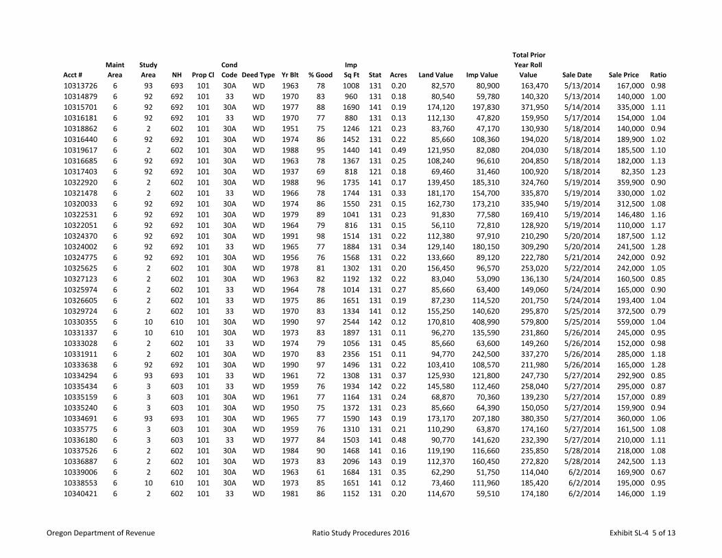
Acct #
Maint
Area
Study
Area NH Prop Cl
Cond
Code Deed Type Yr Blt % Good
Imp
Sq Ft Stat Acres Land Value Imp Value
Total Prior
Year Roll
Value Sale Date Sale Price Ratio
10313726 6 93 693 101 30A WD 1963 78 1008 131 0.20 82,570 80,900 163,470 5/13/2014 167,000 0.98
10314879 6 92 692 101 33 WD 1970 83 960 131 0.18 80,540 59,780 140,320 5/13/2014 140,000 1.00
10315701 6 92 692 101 30A WD 1977 88 1690 141 0.19 174,120 197,830 371,950 5/14/2014 335,000 1.11
10316181 6 92 692 101 33 WD 1970 77 880 131 0.13 112,130 47,820 159,950 5/17/2014 154,000 1.04
10318862 6 2 602 101 30A WD 1951 75 1246 121 0.23 83,760 47,170 130,930 5/18/2014 140,000 0.94
10316440 6 92 692 101 30A WD 1974 86 1452 131 0.22 85,660 108,360 194,020 5/18/2014 189,900 1.02
10319617 6 2 602 101 30A WD 1988 95 1440 141 0.49 121,950 82,080 204,030 5/18/2014 185,500 1.10
10316685 6 92 692 101 30A WD 1963 78 1367 131 0.25 108,240 96,610 204,850 5/18/2014 182,000 1.13
10317403 6 92 692 101 30A WD 1937 69 818 121 0.18 69,460 31,460 100,920 5/18/2014 82,350 1.23
10322920 6 2 602 101 30A WD 1988 96 1735 141 0.17 139,450 185,310 324,760 5/19/2014 359,900 0.90
10321478 6 2 602 101 33 WD 1966 78 1744 131 0.33 181,170 154,700 335,870 5/19/2014 330,000 1.02
10320033 6 92 692 101 30A WD 1974 86 1550 231 0.15 162,730 173,210 335,940 5/19/2014 312,500 1.08
10322531 6 92 692 101 30A WD 1979 89 1041 131 0.23 91,830 77,580 169,410 5/19/2014 146,480 1.16
10322051 6 92 692 101 30A WD 1964 79 816 131 0.15 56,110 72,810 128,920 5/19/2014 110,000 1.17
10324370 6 92 692 101 30A WD 1991 98 1514 131 0.22 112,380 97,910 210,290 5/20/2014 187,500 1.12
10324002 6 92 692 101 33 WD 1965 77 1884 131 0.34 129,140 180,150 309,290 5/20/2014 241,500 1.28
10324775 6 92 692 101 30A WD 1956 76 1568 131 0.22 133,660 89,120 222,780 5/21/2014 242,000 0.92
10325625 6 2 602 101 30A WD 1978 81 1302 131 0.20 156,450 96,570 253,020 5/22/2014 242,000 1.05
10327123 6 2 602 101 30A WD 1963 82 1192 132 0.22 83,040 53,090 136,130 5/24/2014 160,500 0.85
10325974 6 2 602 101 33 WD 1964 78 1014 131 0.27 85,660 63,400 149,060 5/24/2014 165,000 0.90
10326605 6 2 602 101 33 WD 1975 86 1651 131 0.19 87,230 114,520 201,750 5/24/2014 193,400 1.04
10329724 6 2 602 101 33 WD 1970 83 1334 141 0.12 155,250 140,620 295,870 5/25/2014 372,500 0.79
10330355 6 10 610 101 30A WD 1990 97 2544 142 0.12 170,810 408,990 579,800 5/25/2014 559,000 1.04
10331337 6 10 610 101 30A WD 1973 83 1897 131 0.11 96,270 135,590 231,860 5/26/2014 245,000 0.95
10333028 6 2 602 101 33 WD 1974 79 1056 131 0.45 85,660 63,600 149,260 5/26/2014 152,000 0.98
10331911 6 2 602 101 30A WD 1970 83 2356 151 0.11 94,770 242,500 337,270 5/26/2014 285,000 1.18
10333638 6 92 692 101 30A WD 1990 97 1496 131 0.22 103,410 108,570 211,980 5/26/2014 165,000 1.28
10334294 6 93 693 101 33 WD 1961 72 1308 131 0.37 125,930 121,800 247,730 5/27/2014 292,900 0.85
10335434 6 3 603 101 33 WD 1959 76 1934 142 0.22 145,580 112,460 258,040 5/27/2014 295,000 0.87
10335159 6 3 603 101 30A WD 1961 77 1164 131 0.24 68,870 70,360 139,230 5/27/2014 157,000 0.89
10335240 6 3 603 101 30A WD 1950 75 1372 131 0.23 85,660 64,390 150,050 5/27/2014 159,900 0.94
10334691 6 93 693 101 30A WD 1965 77 1590 143 0.19 173,170 207,180 380,350 5/27/2014 360,000 1.06
10335775 6 3 603 101 30A WD 1959 76 1310 131 0.21 110,290 63,870 174,160 5/27/2014 161,500 1.08
10336180 6 3 603 101 33 WD 1977 84 1503 141 0.48 90,770 141,620 232,390 5/27/2014 210,000 1.11
10337526 6 2 602 101 30A WD 1984 90 1468 141 0.16 119,190 116,660 235,850 5/28/2014 218,000 1.08
10336887 6 2 602 101 30A WD 1973 83 2096 143 0.19 112,370 160,450 272,820 5/28/2014 242,500 1.13
10339006 6 2 602 101 30A WD 1963 61 1684 131 0.35 62,290 51,750 114,040 6/2/2014 169,900 0.67
10338553 6 10 610 101 30A WD 1973 85 1651 141 0.12 73,460 111,960 185,420 6/2/2014 195,000 0.95
10340421 6 2 602 101 33 WD 1981 86 1152 131 0.20 114,670 59,510 174,180 6/2/2014 146,000 1.19
Oregon Department of Revenue Ratio Study Procedures 2016 Exhibit SL‐4 5 of 13
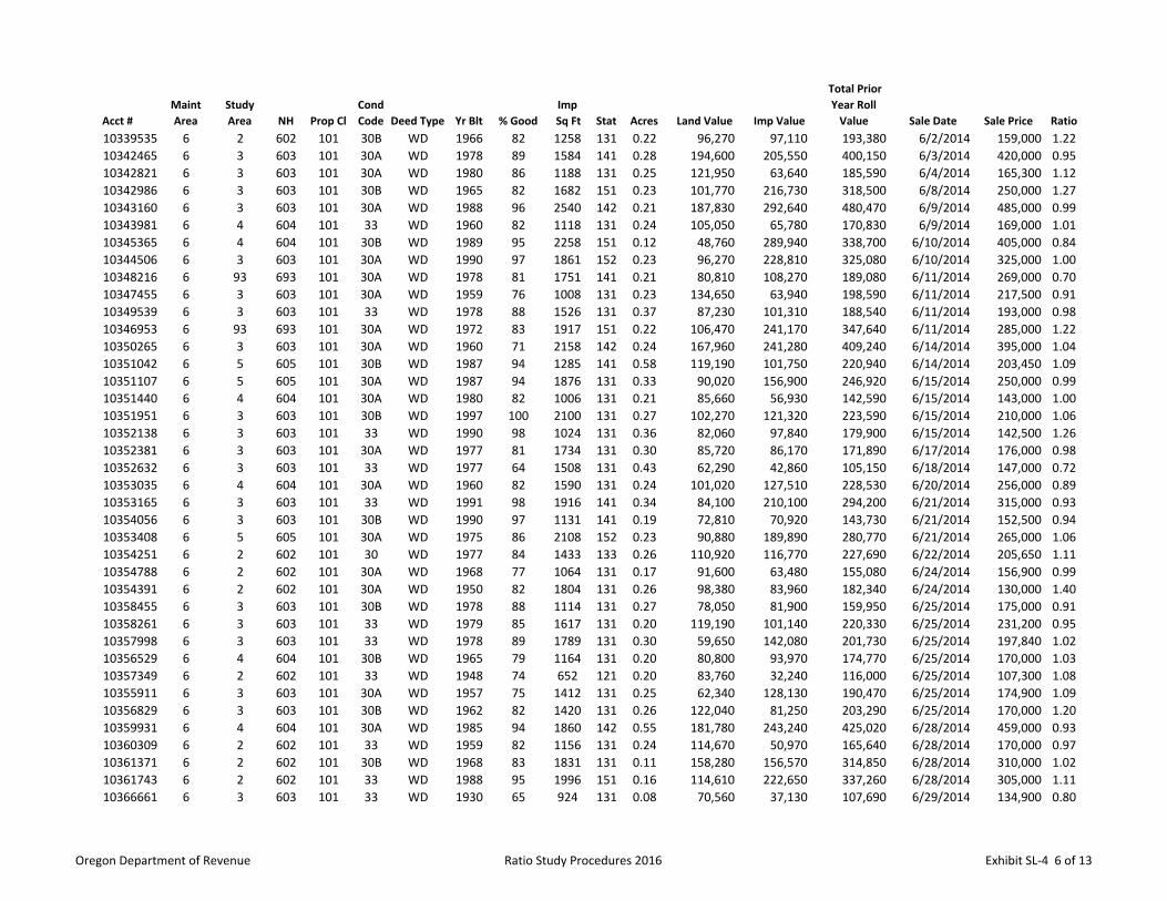
Acct #
Maint
Area
Study
Area NH Prop Cl
Cond
Code Deed Type Yr Blt % Good
Imp
Sq Ft Stat Acres Land Value Imp Value
Total Prior
Year Roll
Value Sale Date Sale Price Ratio
10339535 6 2 602 101 30B WD 1966 82 1258 131 0.22 96,270 97,110 193,380 6/2/2014 159,000 1.22
10342465 6 3 603 101 30A WD 1978 89 1584 141 0.28 194,600 205,550 400,150 6/3/2014 420,000 0.95
10342821 6 3 603 101 30A WD 1980 86 1188 131 0.25 121,950 63,640 185,590 6/4/2014 165,300 1.12
10342986 6 3 603 101 30B WD 1965 82 1682 151 0.23 101,770 216,730 318,500 6/8/2014 250,000 1.27
10343160 6 3 603 101 30A WD 1988 96 2540 142 0.21 187,830 292,640 480,470 6/9/2014 485,000 0.99
10343981 6 4 604 101 33 WD 1960 82 1118 131 0.24 105,050 65,780 170,830 6/9/2014 169,000 1.01
10345365 6 4 604 101 30B WD 1989 95 2258 151 0.12 48,760 289,940 338,700 6/10/2014 405,000 0.84
10344506 6 3 603 101 30A WD 1990 97 1861 152 0.23 96,270 228,810 325,080 6/10/2014 325,000 1.00
10348216 6 93 693 101 30A WD 1978 81 1751 141 0.21 80,810 108,270 189,080 6/11/2014 269,000 0.70
10347455 6 3 603 101 30A WD 1959 76 1008 131 0.23 134,650 63,940 198,590 6/11/2014 217,500 0.91
10349539 6 3 603 101 33 WD 1978 88 1526 131 0.37 87,230 101,310 188,540 6/11/2014 193,000 0.98
10346953 6 93 693 101 30A WD 1972 83 1917 151 0.22 106,470 241,170 347,640 6/11/2014 285,000 1.22
10350265 6 3 603 101 30A WD 1960 71 2158 142 0.24 167,960 241,280 409,240 6/14/2014 395,000 1.04
10351042 6 5 605 101 30B WD 1987 94 1285 141 0.58 119,190 101,750 220,940 6/14/2014 203,450 1.09
10351107 6 5 605 101 30A WD 1987 94 1876 131 0.33 90,020 156,900 246,920 6/15/2014 250,000 0.99
10351440 6 4 604 101 30A WD 1980 82 1006 131 0.21 85,660 56,930 142,590 6/15/2014 143,000 1.00
10351951 6 3 603 101 30B WD 1997 100 2100 131 0.27 102,270 121,320 223,590 6/15/2014 210,000 1.06
10352138 6 3 603 101 33 WD 1990 98 1024 131 0.36 82,060 97,840 179,900 6/15/2014 142,500 1.26
10352381 6 3 603 101 30A WD 1977 81 1734 131 0.30 85,720 86,170 171,890 6/17/2014 176,000 0.98
10352632 6 3 603 101 33 WD 1977 64 1508 131 0.43 62,290 42,860 105,150 6/18/2014 147,000 0.72
10353035 6 4 604 101 30A WD 1960 82 1590 131 0.24 101,020 127,510 228,530 6/20/2014 256,000 0.89
10353165 6 3 603 101 33 WD 1991 98 1916 141 0.34 84,100 210,100 294,200 6/21/2014 315,000 0.93
10354056 6 3 603 101 30B WD 1990 97 1131 141 0.19 72,810 70,920 143,730 6/21/2014 152,500 0.94
10353408 6 5 605 101 30A WD 1975 86 2108 152 0.23 90,880 189,890 280,770 6/21/2014 265,000 1.06
10354251 6 2 602 101 30 WD 1977 84 1433 133 0.26 110,920 116,770 227,690 6/22/2014 205,650 1.11
10354788 6 2 602 101 30A WD 1968 77 1064 131 0.17 91,600 63,480 155,080 6/24/2014 156,900 0.99
10354391 6 2 602 101 30A WD 1950 82 1804 131 0.26 98,380 83,960 182,340 6/24/2014 130,000 1.40
10358455 6 3 603 101 30B WD 1978 88 1114 131 0.27 78,050 81,900 159,950 6/25/2014 175,000 0.91
10358261 6 3 603 101 33 WD 1979 85 1617 131 0.20 119,190 101,140 220,330 6/25/2014 231,200 0.95
10357998 6 3 603 101 33 WD 1978 89 1789 131 0.30 59,650 142,080 201,730 6/25/2014 197,840 1.02
10356529 6 4 604 101 30B WD 1965 79 1164 131 0.20 80,800 93,970 174,770 6/25/2014 170,000 1.03
10357349 6 2 602 101 33 WD 1948 74 652 121 0.20 83,760 32,240 116,000 6/25/2014 107,300 1.08
10355911 6 3 603 101 30A WD 1957 75 1412 131 0.25 62,340 128,130 190,470 6/25/2014 174,900 1.09
10356829 6 3 603 101 30B WD 1962 82 1420 131 0.26 122,040 81,250 203,290 6/25/2014 170,000 1.20
10359931 6 4 604 101 30A WD 1985 94 1860 142 0.55 181,780 243,240 425,020 6/28/2014 459,000 0.93
10360309 6 2 602 101 33 WD 1959 82 1156 131 0.24 114,670 50,970 165,640 6/28/2014 170,000 0.97
10361371 6 2 602 101 30B WD 1968 83 1831 131 0.11 158,280 156,570 314,850 6/28/2014 310,000 1.02
10361743 6 2 602 101 33 WD 1988 95 1996 151 0.16 114,610 222,650 337,260 6/28/2014 305,000 1.11
10366661 6 3 603 101 33 WD 1930 65 924 131 0.08 70,560 37,130 107,690 6/29/2014 134,900 0.80
Oregon Department of Revenue Ratio Study Procedures 2016 Exhibit SL‐4 6 of 13
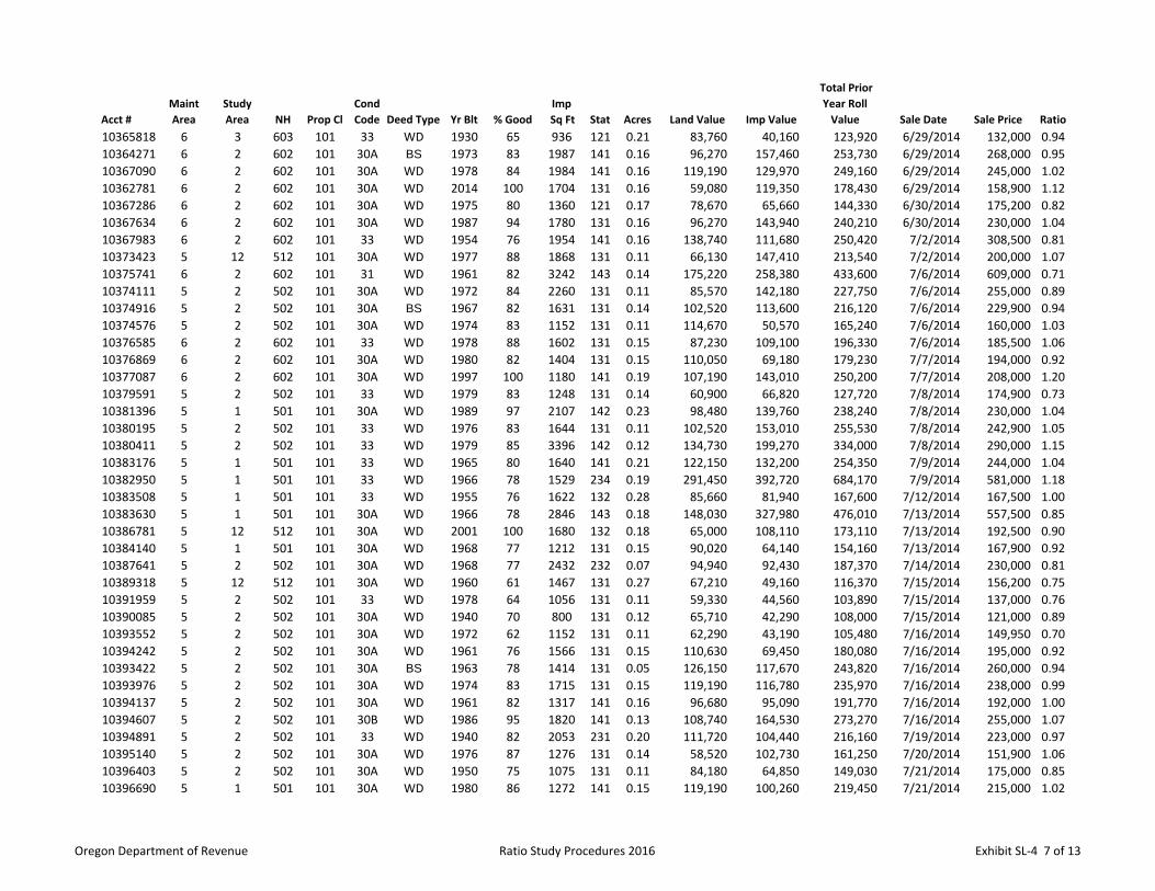
Acct #
Maint
Area
Study
Area NH Prop Cl
Cond
Code Deed Type Yr Blt % Good
Imp
Sq Ft Stat Acres Land Value Imp Value
Total Prior
Year Roll
Value Sale Date Sale Price Ratio
10365818 6 3 603 101 33 WD 1930 65 936 121 0.21 83,760 40,160 123,920 6/29/2014 132,000 0.94
10364271 6 2 602 101 30A BS 1973 83 1987 141 0.16 96,270 157,460 253,730 6/29/2014 268,000 0.95
10367090 6 2 602 101 30A WD 1978 84 1984 141 0.16 119,190 129,970 249,160 6/29/2014 245,000 1.02
10362781 6 2 602 101 30A WD 2014 100 1704 131 0.16 59,080 119,350 178,430 6/29/2014 158,900 1.12
10367286 6 2 602 101 30A WD 1975 80 1360 121 0.17 78,670 65,660 144,330 6/30/2014 175,200 0.82
10367634 6 2 602 101 30A WD 1987 94 1780 131 0.16 96,270 143,940 240,210 6/30/2014 230,000 1.04
10367983 6 2 602 101 33 WD 1954 76 1954 141 0.16 138,740 111,680 250,420 7/2/2014 308,500 0.81
10373423 5 12 512 101 30A WD 1977 88 1868 131 0.11 66,130 147,410 213,540 7/2/2014 200,000 1.07
10375741 6 2 602 101 31 WD 1961 82 3242 143 0.14 175,220 258,380 433,600 7/6/2014 609,000 0.71
10374111 5 2 502 101 30A WD 1972 84 2260 131 0.11 85,570 142,180 227,750 7/6/2014 255,000 0.89
10374916 5 2 502 101 30A BS 1967 82 1631 131 0.14 102,520 113,600 216,120 7/6/2014 229,900 0.94
10374576 5 2 502 101 30A WD 1974 83 1152 131 0.11 114,670 50,570 165,240 7/6/2014 160,000 1.03
10376585 6 2 602 101 33 WD 1978 88 1602 131 0.15 87,230 109,100 196,330 7/6/2014 185,500 1.06
10376869 6 2 602 101 30A WD 1980 82 1404 131 0.15 110,050 69,180 179,230 7/7/2014 194,000 0.92
10377087 6 2 602 101 30A WD 1997 100 1180 141 0.19 107,190 143,010 250,200 7/7/2014 208,000 1.20
10379591 5 2 502 101 33 WD 1979 83 1248 131 0.14 60,900 66,820 127,720 7/8/2014 174,900 0.73
10381396 5 1 501 101 30A WD 1989 97 2107 142 0.23 98,480 139,760 238,240 7/8/2014 230,000 1.04
10380195 5 2 502 101 33 WD 1976 83 1644 131 0.11 102,520 153,010 255,530 7/8/2014 242,900 1.05
10380411 5 2 502 101 33 WD 1979 85 3396 142 0.12 134,730 199,270 334,000 7/8/2014 290,000 1.15
10383176 5 1 501 101 33 WD 1965 80 1640 141 0.21 122,150 132,200 254,350 7/9/2014 244,000 1.04
10382950 5 1 501 101 33 WD 1966 78 1529 234 0.19 291,450 392,720 684,170 7/9/2014 581,000 1.18
10383508 5 1 501 101 33 WD 1955 76 1622 132 0.28 85,660 81,940 167,600 7/12/2014 167,500 1.00
10383630 5 1 501 101 30A WD 1966 78 2846 143 0.18 148,030 327,980 476,010 7/13/2014 557,500 0.85
10386781 5 12 512 101 30A WD 2001 100 1680 132 0.18 65,000 108,110 173,110 7/13/2014 192,500 0.90
10384140 5 1 501 101 30A WD 1968 77 1212 131 0.15 90,020 64,140 154,160 7/13/2014 167,900 0.92
10387641 5 2 502 101 30A WD 1968 77 2432 232 0.07 94,940 92,430 187,370 7/14/2014 230,000 0.81
10389318 5 12 512 101 30A WD 1960 61 1467 131 0.27 67,210 49,160 116,370 7/15/2014 156,200 0.75
10391959 5 2 502 101 33 WD 1978 64 1056 131 0.11 59,330 44,560 103,890 7/15/2014 137,000 0.76
10390085 5 2 502 101 30A WD 1940 70 800 131 0.12 65,710 42,290 108,000 7/15/2014 121,000 0.89
10393552 5 2 502 101 30A WD 1972 62 1152 131 0.11 62,290 43,190 105,480 7/16/2014 149,950 0.70
10394242 5 2 502 101 30A WD 1961 76 1566 131 0.15 110,630 69,450 180,080 7/16/2014 195,000 0.92
10393422 5 2 502 101 30A BS 1963 78 1414 131 0.05 126,150 117,670 243,820 7/16/2014 260,000 0.94
10393976 5 2 502 101 30A WD 1974 83 1715 131 0.15 119,190 116,780 235,970 7/16/2014 238,000 0.99
10394137 5 2 502 101 30A WD 1961 82 1317 141 0.16 96,680 95,090 191,770 7/16/2014 192,000 1.00
10394607 5 2 502 101 30B WD 1986 95 1820 141 0.13 108,740 164,530 273,270 7/16/2014 255,000 1.07
10394891 5 2 502 101 33 WD 1940 82 2053 231 0.20 111,720 104,440 216,160 7/19/2014 223,000 0.97
10395140 5 2 502 101 30A WD 1976 87 1276 131 0.14 58,520 102,730 161,250 7/20/2014 151,900 1.06
10396403 5 2 502 101 30A WD 1950 75 1075 131 0.11 84,180 64,850 149,030 7/21/2014 175,000 0.85
10396690 5 1 501 101 30A WD 1980 86 1272 141 0.15 119,190 100,260 219,450 7/21/2014 215,000 1.02
Oregon Department of Revenue Ratio Study Procedures 2016 Exhibit SL‐4 7 of 13
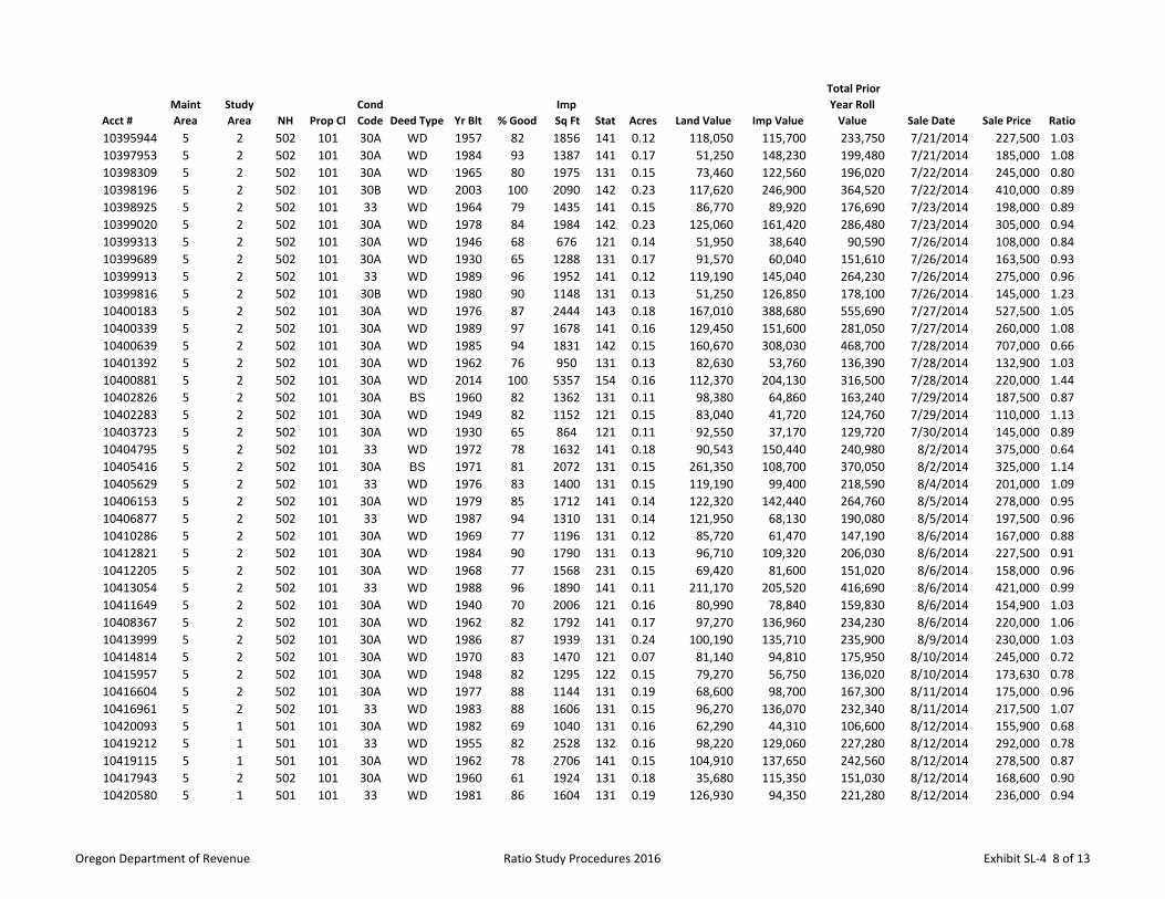
Acct #
Maint
Area
Study
Area NH Prop Cl
Cond
Code Deed Type Yr Blt % Good
Imp
Sq Ft Stat Acres Land Value Imp Value
Total Prior
Year Roll
Value Sale Date Sale Price Ratio
10395944 5 2 502 101 30A WD 1957 82 1856 141 0.12 118,050 115,700 233,750 7/21/2014 227,500 1.03
10397953 5 2 502 101 30A WD 1984 93 1387 141 0.17 51,250 148,230 199,480 7/21/2014 185,000 1.08
10398309 5 2 502 101 30A WD 1965 80 1975 131 0.15 73,460 122,560 196,020 7/22/2014 245,000 0.80
10398196 5 2 502 101 30B WD 2003 100 2090 142 0.23 117,620 246,900 364,520 7/22/2014 410,000 0.89
10398925 5 2 502 101 33 WD 1964 79 1435 141 0.15 86,770 89,920 176,690 7/23/2014 198,000 0.89
10399020 5 2 502 101 30A WD 1978 84 1984 142 0.23 125,060 161,420 286,480 7/23/2014 305,000 0.94
10399313 5 2 502 101 30A WD 1946 68 676 121 0.14 51,950 38,640 90,590 7/26/2014 108,000 0.84
10399689 5 2 502 101 30A WD 1930 65 1288 131 0.17 91,570 60,040 151,610 7/26/2014 163,500 0.93
10399913 5 2 502 101 33 WD 1989 96 1952 141 0.12 119,190 145,040 264,230 7/26/2014 275,000 0.96
10399816 5 2 502 101 30B WD 1980 90 1148 131 0.13 51,250 126,850 178,100 7/26/2014 145,000 1.23
10400183 5 2 502 101 30A WD 1976 87 2444 143 0.18 167,010 388,680 555,690 7/27/2014 527,500 1.05
10400339 5 2 502 101 30A WD 1989 97 1678 141 0.16 129,450 151,600 281,050 7/27/2014 260,000 1.08
10400639 5 2 502 101 30A WD 1985 94 1831 142 0.15 160,670 308,030 468,700 7/28/2014 707,000 0.66
10401392 5 2 502 101 30A WD 1962 76 950 131 0.13 82,630 53,760 136,390 7/28/2014 132,900 1.03
10400881 5 2 502 101 30A WD 2014 100 5357 154 0.16 112,370 204,130 316,500 7/28/2014 220,000 1.44
10402826 5 2 502 101 30A BS 1960 82 1362 131 0.11 98,380 64,860 163,240 7/29/2014 187,500 0.87
10402283 5 2 502 101 30A WD 1949 82 1152 121 0.15 83,040 41,720 124,760 7/29/2014 110,000 1.13
10403723 5 2 502 101 30A WD 1930 65 864 121 0.11 92,550 37,170 129,720 7/30/2014 145,000 0.89
10404795 5 2 502 101 33 WD 1972 78 1632 141 0.18 90,543 150,440 240,980 8/2/2014 375,000 0.64
10405416 5 2 502 101 30A BS 1971 81 2072 131 0.15 261,350 108,700 370,050 8/2/2014 325,000 1.14
10405629 5 2 502 101 33 WD 1976 83 1400 131 0.15 119,190 99,400 218,590 8/4/2014 201,000 1.09
10406153 5 2 502 101 30A WD 1979 85 1712 141 0.14 122,320 142,440 264,760 8/5/2014 278,000 0.95
10406877 5 2 502 101 33 WD 1987 94 1310 131 0.14 121,950 68,130 190,080 8/5/2014 197,500 0.96
10410286 5 2 502 101 30A WD 1969 77 1196 131 0.12 85,720 61,470 147,190 8/6/2014 167,000 0.88
10412821 5 2 502 101 30A WD 1984 90 1790 131 0.13 96,710 109,320 206,030 8/6/2014 227,500 0.91
10412205 5 2 502 101 30A WD 1968 77 1568 231 0.15 69,420 81,600 151,020 8/6/2014 158,000 0.96
10413054 5 2 502 101 33 WD 1988 96 1890 141 0.11 211,170 205,520 416,690 8/6/2014 421,000 0.99
10411649 5 2 502 101 30A WD 1940 70 2006 121 0.16 80,990 78,840 159,830 8/6/2014 154,900 1.03
10408367 5 2 502 101 30A WD 1962 82 1792 141 0.17 97,270 136,960 234,230 8/6/2014 220,000 1.06
10413999 5 2 502 101 30A WD 1986 87 1939 131 0.24 100,190 135,710 235,900 8/9/2014 230,000 1.03
10414814 5 2 502 101 30A WD 1970 83 1470 121 0.07 81,140 94,810 175,950 8/10/2014 245,000 0.72
10415957 5 2 502 101 30A WD 1948 82 1295 122 0.15 79,270 56,750 136,020 8/10/2014 173,630 0.78
10416604 5 2 502 101 30A WD 1977 88 1144 131 0.19 68,600 98,700 167,300 8/11/2014 175,000 0.96
10416961 5 2 502 101 33 WD 1983 88 1606 131 0.15 96,270 136,070 232,340 8/11/2014 217,500 1.07
10420093 5 1 501 101 30A WD 1982 69 1040 131 0.16 62,290 44,310 106,600 8/12/2014 155,900 0.68
10419212 5 1 501 101 33 WD 1955 82 2528 132 0.16 98,220 129,060 227,280 8/12/2014 292,000 0.78
10419115 5 1 501 101 30A WD 1962 78 2706 141 0.15 104,910 137,650 242,560 8/12/2014 278,500 0.87
10417943 5 2 502 101 30A WD 1960 61 1924 131 0.18 35,680 115,350 151,030 8/12/2014 168,600 0.90
10420580 5 1 501 101 33 WD 1981 86 1604 131 0.19 126,930 94,350 221,280 8/12/2014 236,000 0.94
Oregon Department of Revenue Ratio Study Procedures 2016 Exhibit SL‐4 8 of 13

Acct #
Maint
Area
Study
Area NH Prop Cl
Cond
Code Deed Type Yr Blt % Good
Imp
Sq Ft Stat Acres Land Value Imp Value
Total Prior
Year Roll
Value Sale Date Sale Price Ratio
10418450 5 1 501 101 30A WD 1999 100 2440 162 0.35 305,900 334,190 640,090 8/12/2014 675,000 0.95
10420871 5 2 502 101 33 WD 1990 98 1272 131 0.19 71,050 125,600 196,650 8/12/2014 199,000 0.99
10421721 5 2 502 101 33 WD 1963 78 2090 131 0.19 78,050 90,120 168,170 8/13/2014 188,000 0.89
10423149 6 2 602 101 30A WD 1945 82 1382 121 0.26 98,380 36,280 134,660 8/16/2014 169,000 0.80
10421837 5 1 501 101 33 WD 1957 75 836 131 0.20 41,560 82,090 123,650 8/16/2014 147,900 0.84
10424111 6 3 603 101 30A WD 1973 79 1365 131 1.20 91,600 80,450 172,050 8/16/2014 184,000 0.94
10426365 6 3 603 101 30A WD 1990 95 1200 131 0.48 85,720 86,690 172,410 8/16/2014 175,000 0.99
10429750 5 7 507 101 33 WD 1955 82 2256 143 0.70 90,770 153,550 244,320 8/17/2014 300,000 0.81
10430104 5 7 507 101 30A WD 1950 82 955 131 0.36 109,750 65,860 175,610 8/17/2014 159,000 1.10
10431768 5 7 507 101 30A WD 1959 82 1404 131 0.29 96,380 82,030 178,410 8/18/2014 199,400 0.89
10431508 5 7 507 101 30A WD 2001 100 1444 131 0.23 59,980 156,100 216,080 8/18/2014 220,000 0.98
10432247 5 7 507 101 30A WD 1982 92 1311 131 0.34 90,250 103,960 194,210 8/18/2014 192,000 1.01
10433574 5 7 507 101 33 WD 2000 100 3825 142 0.40 152,950 249,860 402,810 8/19/2014 539,000 0.75
10434554 5 7 507 101 30A WD 1966 80 2170 133 0.60 79,000 157,090 236,090 8/19/2014 244,000 0.97
10435486 5 7 507 101 30A WD 1988 95 2438 152 1.02 96,270 325,260 421,530 8/19/2014 420,000 1.00
10436474 5 7 507 101 30A WD 1980 86 1364 131 0.35 121,950 65,380 187,330 8/23/2014 181,000 1.03
10438661 5 7 507 101 33 WD 1957 82 1252 131 0.38 94,040 73,140 167,180 8/24/2014 160,000 1.04
10437032 5 7 507 101 30A WD 1969 83 1004 131 0.29 121,950 46,360 168,310 8/24/2014 150,000 1.12
10439579 5 7 507 101 30A WD 1977 84 1370 141 0.25 89,270 128,240 217,510 8/24/2014 193,000 1.13
10443983 5 1 501 101 33 WD 1953 76 948 131 0.28 76,400 56,660 133,060 8/25/2014 155,000 0.86
10443462 5 7 507 101 30A WD 1960 71 1026 131 0.51 134,470 99,410 233,880 8/25/2014 250,000 0.94
10448868 5 7 507 101 33 WD 1978 64 1152 131 0.50 67,210 45,850 113,060 8/26/2014 162,500 0.70
10449159 5 7 507 101 30A WD 1977 84 1413 131 0.29 112,850 61,170 174,020 8/26/2014 214,900 0.81
10449726 5 7 507 101 30A WD 1962 76 1088 131 0.27 85,720 59,600 145,320 8/26/2014 168,000 0.87
10452601 5 1 501 101 30A WD 1980 86 1188 131 0.14 121,950 55,540 177,490 8/26/2014 193,500 0.92
10455209 5 7 507 101 33 WD 1972 78 1920 231 0.37 85,610 79,270 164,880 8/27/2014 180,000 0.92
10486508 5 1 501 101 30A WD 1989 96 1902 131 0.16 119,190 117,380 236,570 8/27/2014 240,000 0.99
10474480 5 4 504 101 30A WD 1977 84 1843 131 1.00 96,270 161,750 258,020 8/27/2014 243,000 1.06
10454156 5 7 507 101 30A WD 1999 100 2281 152 1.05 134,470 417,250 551,720 8/27/2014 462,998 1.19
10487853 5 1 501 101 30A WD 1968 77 1222 131 0.16 84,180 69,540 153,720 8/30/2014 176,500 0.87
10488980 5 1 501 101 30A WD 1972 81 1100 141 0.18 60,900 80,140 141,040 8/31/2014 157,500 0.90
10489481 5 1 501 101 30A WD 1988 80 1548 131 0.50 41,880 158,290 200,170 8/31/2014 170,850 1.17
10490136 5 1 501 101 30A WD 1990 97 2478 151 0.20 152,910 314,280 467,190 9/2/2014 443,000 1.05
10490004 5 1 501 101 33 WD 1979 82 1490 141 0.15 157,480 94,150 251,630 9/2/2014 214,000 1.18
10490451 5 1 501 101 30A WD 1953 72 1676 121 0.11 111,300 89,510 200,810 9/3/2014 242,000 0.83
10490777 5 1 501 101 33 WD 1964 76 1260 131 0.39 159,370 92,800 252,170 9/4/2014 249,000 1.01
10492228 5 12 512 101 33 WD 2001 100 2141 141 0.13 122,040 158,820 280,860 9/7/2014 325,500 0.86
10493036 5 1 501 101 30A WD 1995 100 1224 131 0.18 49,090 135,600 184,690 9/10/2014 208,000 0.89
10494245 5 1 501 101 33 WD 1958 82 1552 131 0.16 111,380 92,000 203,380 9/13/2014 269,000 0.76
Oregon Department of Revenue Ratio Study Procedures 2016 Exhibit SL‐4 9 of 13
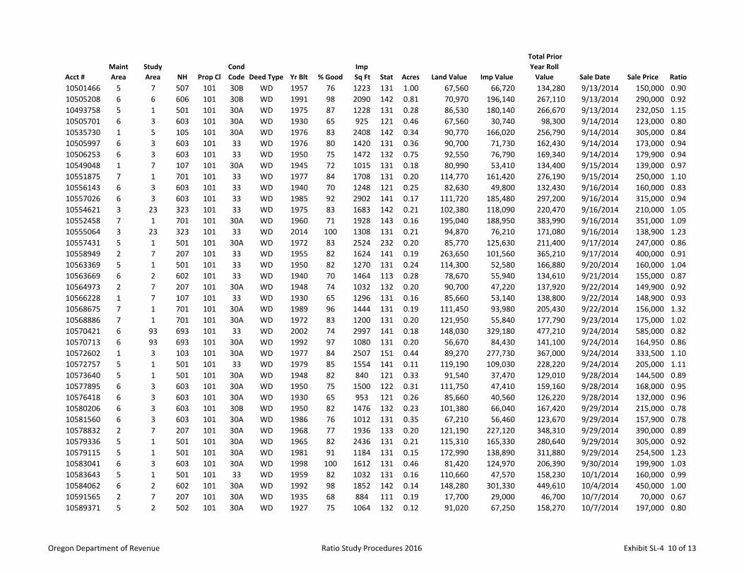
Acct #
Maint
Area
Study
Area NH Prop Cl
Cond
Code Deed Type Yr Blt % Good
Imp
Sq Ft Stat Acres Land Value Imp Value
Total Prior
Year Roll
Value Sale Date Sale Price Ratio
10501466 5 7 507 101 30B WD 1957 76 1223 131 1.00 67,560 66,720 134,280 9/13/2014 150,000 0.90
10505208 6 6 606 101 30B WD 1991 98 2090 142 0.81 70,970 196,140 267,110 9/13/2014 290,000 0.92
10493758 5 1 501 101 30A WD 1975 87 1228 131 0.28 86,530 180,140 266,670 9/13/2014 232,050 1.15
10505701 6 3 603 101 30A WD 1930 65 925 121 0.46 67,560 30,740 98,300 9/14/2014 123,000 0.80
10535730 1 5 105 101 30A WD 1976 83 2408 142 0.34 90,770 166,020 256,790 9/14/2014 305,000 0.84
10505997 6 3 603 101 33 WD 1976 80 1420 131 0.36 90,700 71,730 162,430 9/14/2014 173,000 0.94
10506253 6 3 603 101 33 WD 1950 75 1472 132 0.75 92,550 76,790 169,340 9/14/2014 179,900 0.94
10549048 1 7 107 101 30A WD 1945 72 1015 131 0.18 80,990 53,410 134,400 9/15/2014 139,000 0.97
10551875 7 1 701 101 33 WD 1977 84 1708 131 0.20 114,770 161,420 276,190 9/15/2014 250,000 1.10
10556143 6 3 603 101 33 WD 1940 70 1248 121 0.25 82,630 49,800 132,430 9/16/2014 160,000 0.83
10557026 6 3 603 101 33 WD 1985 92 2902 141 0.17 111,720 185,480 297,200 9/16/2014 315,000 0.94
10554621 3 23 323 101 33 WD 1975 83 1683 142 0.21 102,380 118,090 220,470 9/16/2014 210,000 1.05
10552458 7 1 701 101 30A WD 1960 71 1928 143 0.16 195,040 188,950 383,990 9/16/2014 351,000 1.09
10555064 3 23 323 101 33 WD 2014 100 1308 131 0.21 94,870 76,210 171,080 9/16/2014 138,900 1.23
10557431 5 1 501 101 30A WD 1972 83 2524 232 0.20 85,770 125,630 211,400 9/17/2014 247,000 0.86
10558949 2 7 207 101 33 WD 1955 82 1624 141 0.19 263,650 101,560 365,210 9/17/2014 400,000 0.91
10563369 5 1 501 101 33 WD 1950 82 1270 131 0.24 114,300 52,580 166,880 9/20/2014 160,000 1.04
10563669 6 2 602 101 33 WD 1940 70 1464 113 0.28 78,670 55,940 134,610 9/21/2014 155,000 0.87
10564973 2 7 207 101 30A WD 1948 74 1032 132 0.20 90,700 47,220 137,920 9/22/2014 149,900 0.92
10566228 1 7 107 101 33 WD 1930 65 1296 131 0.16 85,660 53,140 138,800 9/22/2014 148,900 0.93
10568675 7 1 701 101 30A WD 1989 96 1444 131 0.19 111,450 93,980 205,430 9/22/2014 156,000 1.32
10568886 7 1 701 101 30A WD 1972 83 1200 131 0.20 121,950 55,840 177,790 9/23/2014 175,000 1.02
10570421 6 93 693 101 33 WD 2002 74 2997 141 0.18 148,030 329,180 477,210 9/24/2014 585,000 0.82
10570713 6 93 693 101 30A WD 1992 97 1080 131 0.20 56,670 84,430 141,100 9/24/2014 164,950 0.86
10572602 1 3 103 101 30A WD 1977 84 2507 151 0.44 89,270 277,730 367,000 9/24/2014 333,500 1.10
10572757 5 1 501 101 33 WD 1979 85 1554 141 0.11 119,190 109,030 228,220 9/24/2014 205,000 1.11
10573640 5 1 501 101 30A WD 1948 82 840 121 0.33 91,540 37,470 129,010 9/28/2014 144,500 0.89
10577895 6 3 603 101 30A WD 1950 75 1500 122 0.31 111,750 47,410 159,160 9/28/2014 168,000 0.95
10576418 6 3 603 101 30A WD 1930 65 953 121 0.26 85,660 40,560 126,220 9/28/2014 132,000 0.96
10580206 6 3 603 101 30B WD 1950 82 1476 132 0.23 101,380 66,040 167,420 9/29/2014 215,000 0.78
10581560 6 3 603 101 30A WD 1986 76 1012 131 0.35 67,210 56,460 123,670 9/29/2014 157,900 0.78
10578832 2 7 207 101 30A WD 1968 77 1936 133 0.20 121,190 227,120 348,310 9/29/2014 390,000 0.89
10579336 5 1 501 101 30A WD 1965 82 2436 131 0.21 115,310 165,330 280,640 9/29/2014 305,000 0.92
10579115 5 1 501 101 30A WD 1981 91 1184 131 0.15 172,990 138,890 311,880 9/29/2014 254,500 1.23
10583041 6 3 603 101 30A WD 1998 100 1612 131 0.46 81,420 124,970 206,390 9/30/2014 199,900 1.03
10583643 5 1 501 101 33 WD 1959 82 1032 131 0.16 110,660 47,570 158,230 10/1/2014 160,000 0.99
10584062 6 2 602 101 30A WD 1992 98 1852 142 0.14 148,280 301,330 449,610 10/4/2014 450,000 1.00
10591565 2 7 207 101 30A WD 1935 68 884 111 0.19 17,700 29,000 46,700 10/7/2014 70,000 0.67
10589371 5 2 502 101 30A WD 1927 75 1064 132 0.12 91,020 67,250 158,270 10/7/2014 197,000 0.80
Oregon Department of Revenue Ratio Study Procedures 2016 Exhibit SL‐4 10 of 13

Acct #
Maint
Area
Study
Area NH Prop Cl
Cond
Code Deed Type Yr Blt % Good
Imp
Sq Ft Stat Acres Land Value Imp Value
Total Prior
Year Roll
Value Sale Date Sale Price Ratio
10594408 7 2 702 101 30A WD 1946 73 997 121 0.10 82,010 43,730 125,740 10/7/2014 130,000 0.97
10586235 5 1 501 101 30A WD 1955 79 1711 132 0.35 93,670 70,770 164,440 10/7/2014 162,000 1.02
10594262 7 2 702 101 30A WD 1989 96 1008 131 0.08 103,410 76,080 179,490 10/7/2014 169,000 1.06
10594871 5 1 501 101 30A WD 1972 84 1380 133 0.17 176,200 134,230 310,430 10/8/2014 330,000 0.94
10595631 6 93 693 101 30A WD 1986 95 2661 152 0.23 108,740 271,880 380,620 10/8/2014 376,000 1.01
10595399 6 93 693 101 33 WD 1946 73 1160 122 0.23 83,760 47,070 130,830 10/8/2014 121,000 1.08
10595737 6 93 693 101 30A WD 1985 94 1129 122 0.24 115,260 86,300 201,560 10/11/2014 305,000 0.66
10595981 6 93 693 101 33 WD 1980 90 1008 131 0.23 64,940 61,690 126,630 10/11/2014 136,000 0.93
10596222 6 93 693 101 30A WD 1964 78 2046 131 0.23 47,110 132,350 179,460 10/12/2014 195,000 0.92
10596466 6 93 693 101 30A WD 1963 82 1240 131 0.23 114,670 53,210 167,880 10/13/2014 195,000 0.86
10597318 6 93 693 101 30A WD 1940 70 832 121 0.25 87,930 33,890 121,820 10/13/2014 132,000 0.92
10600181 5 1 501 101 33 WD 1977 84 1208 131 0.42 101,380 79,540 180,920 10/13/2014 187,000 0.97
10601703 2 3 203 101 33 WD 1945 82 1062 131 0.18 104,380 71,270 175,650 10/14/2014 204,500 0.86
10601957 3 23 323 101 30A WD 1988 95 1440 131 0.17 96,040 93,250 189,290 10/14/2014 185,000 1.02
10608567 4 5 405 101 30A WD 1969 81 3900 144 0.17 177,390 792,330 969,720 10/15/2014 1,150,000 0.84
10610656 5 2 502 101 30A WD 1952 82 1298 121 0.16 88,040 64,800 152,840 10/15/2014 172,000 0.89
10613939 3 23 323 101 30A WD 1948 74 1045 121 0.23 111,450 46,030 157,480 10/15/2014 160,000 0.98
10614343 3 23 323 101 30A WD 2003 100 3558 131 0.20 98,960 218,360 317,320 10/15/2014 285,000 1.11
10615654 3 23 323 101 30A WD 1990 97 3736 143 0.20 299,230 402,550 701,780 10/18/2014 950,000 0.74
10615816 3 23 323 101 30A WD 1945 72 1180 132 0.16 69,460 54,400 123,860 10/19/2014 150,000 0.83
10616481 5 1 501 101 30A WD 1966 80 1144 131 0.18 87,230 73,090 160,320 10/20/2014 179,000 0.90
10621891 4 2 402 101 33 WD 1965 76 1411 131 0.14 135,470 83,200 218,670 10/21/2014 289,900 0.75
10617365 6 93 693 101 33 WD 1950 82 840 121 0.23 98,380 38,960 137,340 10/21/2014 177,500 0.77
10616799 5 1 501 101 33 WD 1988 94 1092 131 0.19 42,740 92,750 135,490 10/21/2014 147,900 0.92
10617868 6 93 693 101 33 WD 1971 78 1920 231 0.20 85,610 77,300 162,910 10/21/2014 172,950 0.94
10626508 6 4 604 101 33 WD 1930 65 816 131 0.12 74,510 41,230 115,740 10/25/2014 113,500 1.02
10624831 6 2 602 101 30A WD 1985 94 3586 143 0.19 171,880 438,170 610,050 10/25/2014 465,000 1.31
10628398 1 7 107 101 30A WD 1940 70 792 121 0.15 85,660 36,590 122,250 10/26/2014 144,000 0.85
10627628 4 6 406 101 30A WD 1967 79 1205 131 0.12 178,500 138,280 316,780 10/26/2014 310,000 1.02
10630922 4 11 411 101 33 WD 1960 76 1124 121 0.31 69,420 55,730 125,150 10/27/2014 160,000 0.78
10633409 7 1 701 101 33 WD 1987 95 1104 131 0.19 51,250 105,070 156,320 10/27/2014 176,000 0.89
10632112 1 9 109 101 30A WD 1965 76 1149 131 0.19 92,550 62,960 155,510 10/27/2014 167,000 0.93
10630012 4 11 411 101 30A WD 1949 82 1548 131 0.32 96,710 90,130 186,840 10/27/2014 200,000 0.93
10643178 6 92 692 101 30A WD 1989 96 1520 131 0.21 121,950 73,230 195,180 10/28/2014 219,000 0.89
10634529 6 2 602 101 30A WD 1975 86 2112 133 0.38 47,210 127,120 174,330 10/28/2014 194,900 0.89
10642571 4 2 402 101 33 WD 1965 76 1452 131 0.20 114,070 82,070 196,140 10/28/2014 180,000 1.09
10637494 6 3 603 101 30A WD 1946 68 1012 121 0.35 107,530 40,410 147,940 10/28/2014 131,000 1.13
10638677 4 8 408 101 30A WD 1946 68 1032 121 0.16 105,060 61,580 166,640 10/28/2014 119,500 1.39
10645080 2 3 203 101 30A WD 1989 96 1759 131 0.11 119,190 111,000 230,190 10/29/2014 271,000 0.85
Oregon Department of Revenue Ratio Study Procedures 2016 Exhibit SL‐4 11 of 13
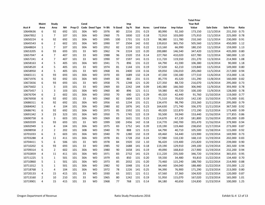
Acct #
Maint
Area
Study
Area NH Prop Cl
Cond
Code Deed Type Yr Blt % Good
Imp
Sq Ft Stat Acres Land Value Imp Value
Total Prior
Year Roll
Value Sale Date Sale Price Ratio
10649636 6 92 692 101 30A WD 1976 80 2216 231 0.23 80,990 92,160 173,150 11/1/2014 231,350 0.75
10647852 1 7 107 101 30A WD 1960 75 1830 122 0.18 72,910 103,000 175,910 11/1/2014 225,000 0.78
10650224 6 92 692 101 30A WD 1995 100 1731 131 0.23 98,380 111,780 210,160 11/1/2014 230,000 0.91
10645543 6 2 602 101 30A WD 1990 97 2504 142 0.02 139,810 365,750 505,560 11/1/2014 450,000 1.12
10648824 1 7 107 101 30A WD 1952 82 1150 131 0.22 113,160 66,990 180,150 11/1/2014 159,000 1.13
10653205 6 93 693 101 33 WD 1962 74 2224 122 0.20 200,880 146,540 347,420 11/2/2014 435,000 0.80
10657047 4 7 407 101 33 WD 1988 96 2320 153 0.14 227,760 410,020 637,780 11/2/2014 580,000 1.10
10657241 4 7 407 101 33 WD 1990 97 1597 141 0.15 111,720 119,550 231,270 11/3/2014 214,900 1.08
10658163 4 5 405 101 30A WD 1941 71 896 131 0.22 64,790 41,590 106,380 11/4/2014 90,000 1.18
10658520 4 5 405 101 33 WD 1974 81 1144 131 0.19 57,630 62,210 119,840 11/5/2014 149,000 0.80
10658950 4 5 405 101 33 WD 1968 81 2400 133 0.16 69,050 136,010 205,060 11/5/2014 217,000 0.94
10665111 6 93 693 101 30A WD 1970 83 1689 132 0.24 47,330 130,180 177,510 11/6/2014 153,000 1.16
10671976 6 92 692 101 30A WD 1949 82 882 231 0.15 85,770 45,520 131,290 11/8/2014 160,000 0.82
10672656 6 93 693 101 33 WD 1958 75 1248 121 0.20 127,350 88,720 216,070 11/9/2014 295,000 0.73
10675602 1 3 103 101 33 WD 1969 83 2242 144 0.09 140,380 166,560 306,940 11/9/2014 393,900 0.78
10675457 1 3 103 101 30A WD 1960 80 896 121 0.11 59,380 40,720 100,100 11/9/2014 128,000 0.78
10676704 6 2 602 101 30A WD 1950 70 690 121 0.29 49,320 42,440 91,760 11/10/2014 119,000 0.77
10676958 6 92 692 101 33 WD 1960 82 1604 121 0.19 71,510 70,620 142,130 11/10/2014 175,000 0.81
10686311 6 92 692 101 30A WD 1956 65 1234 131 0.21 134,470 98,790 233,260 11/11/2014 295,000 0.79
10684042 1 4 104 101 30A WD 1980 82 1876 141 0.23 164,630 171,740 336,370 11/11/2014 367,500 0.92
10686741 6 92 692 101 30A WD 1973 85 1592 131 0.21 49,320 122,870 172,190 11/12/2014 173,400 0.99
10691342 3 23 323 101 30A WD 1950 75 1745 122 0.19 93,500 59,940 153,440 11/16/2014 177,855 0.86
10690758 6 3 603 101 30A WD 1969 83 1631 131 0.23 114,670 67,130 181,800 11/16/2014 205,000 0.89
10692039 6 93 693 101 33 WD 1999 100 2456 142 0.18 114,770 240,700 355,470 11/16/2014 379,900 0.94
10692949 1 4 104 101 30A WD 1975 83 1752 141 0.39 119,190 119,460 238,650 11/17/2014 273,000 0.87
10698958 2 2 202 101 30B WD 1940 70 888 121 0.15 64,790 40,710 105,500 11/18/2014 115,000 0.92
10701033 6 3 603 101 30A WD 1940 70 1280 132 0.19 69,460 54,440 123,900 11/19/2014 169,900 0.73
10703288 4 11 411 101 30A WD 1978 81 1728 232 0.24 57,980 110,130 168,110 11/19/2014 202,000 0.83
10704411 5 6 506 101 33 WD 1978 84 1920 132 1.10 96,420 119,400 215,820 11/19/2014 239,000 0.90
10710202 6 93 693 101 33 WD 1985 92 1688 141 0.18 119,190 129,910 249,100 11/19/2014 265,500 0.94
10709314 6 2 602 101 30A WD 1980 90 1658 141 0.19 49,090 168,810 217,900 11/19/2014 232,200 0.94
10702859 4 11 411 101 30A WD 1971 83 2732 141 0.23 111,220 235,500 346,720 11/19/2014 365,655 0.95
10711225 5 1 501 101 30A WD 1979 65 850 131 0.20 59,330 34,480 93,810 11/22/2014 134,400 0.70
10710860 5 1 501 101 30A WD 1973 85 2032 131 0.20 73,460 115,240 188,700 11/22/2014 214,900 0.88
10711012 5 1 501 101 30A WD 1982 92 1048 131 0.14 84,440 104,040 188,480 11/22/2014 155,000 1.22
10718768 1 4 104 101 30A WD 1972 78 1226 141 0.25 94,390 76,900 171,290 11/23/2014 213,000 0.80
10720133 4 15 415 101 33 WD 1930 65 1021 121 0.11 67,560 37,360 104,920 11/23/2014 120,000 0.87
10713160 2 10 210 101 33 WD 1965 80 1242 131 0.19 51,950 115,070 167,020 11/23/2014 165,000 1.01
10719901 4 15 415 101 33 WD 1968 77 768 121 0.14 84,180 40,650 124,830 11/23/2014 100,000 1.25
Oregon Department of Revenue Ratio Study Procedures 2016 Exhibit SL‐4 12 of 13
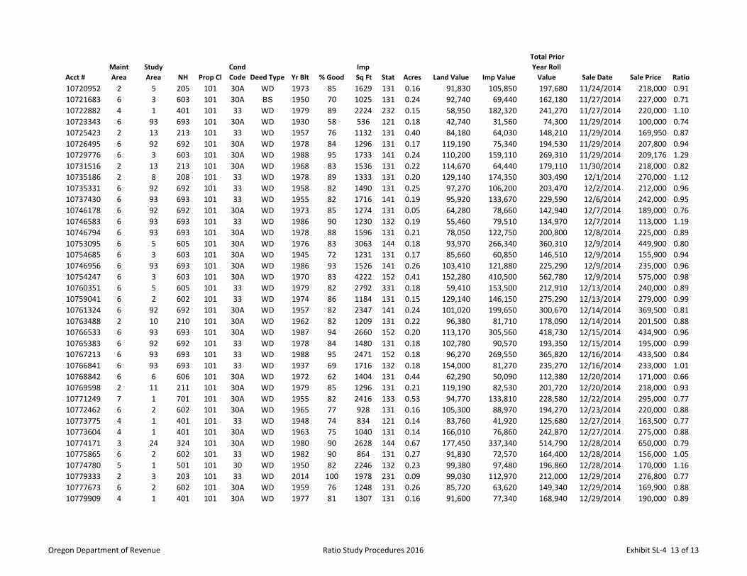
Acct #
Maint
Area
Study
Area NH Prop Cl
Cond
Code Deed Type Yr Blt % Good
Imp
Sq Ft Stat Acres Land Value Imp Value
Total Prior
Year Roll
Value Sale Date Sale Price Ratio
10720952 2 5 205 101 30A WD 1973 85 1629 131 0.16 91,830 105,850 197,680 11/24/2014 218,000 0.91
10721683 6 3 603 101 30A BS 1950 70 1025 131 0.24 92,740 69,440 162,180 11/27/2014 227,000 0.71
10722882 4 1 401 101 33 WD 1979 89 2224 232 0.15 58,950 182,320 241,270 11/27/2014 220,000 1.10
10723343 6 93 693 101 30A WD 1930 58 536 121 0.18 42,740 31,560 74,300 11/29/2014 100,000 0.74
10725423 2 13 213 101 33 WD 1957 76 1132 131 0.40 84,180 64,030 148,210 11/29/2014 169,950 0.87
10726495 6 92 692 101 30A WD 1978 84 1296 131 0.17 119,190 75,340 194,530 11/29/2014 207,800 0.94
10729776 6 3 603 101 30A WD 1988 95 1733 141 0.24 110,200 159,110 269,310 11/29/2014 209,176 1.29
10731516 2 13 213 101 30A WD 1968 83 1536 131 0.22 114,670 64,440 179,110 11/30/2014 218,000 0.82
10735186 2 8 208 101 33 WD 1978 89 1333 131 0.20 129,140 174,350 303,490 12/1/2014 270,000 1.12
10735331 6 92 692 101 33 WD 1958 82 1490 131 0.25 97,270 106,200 203,470 12/2/2014 212,000 0.96
10737430 6 93 693 101 33 WD 1955 82 1716 141 0.19 95,920 133,670 229,590 12/6/2014 242,000 0.95
10746178 6 92 692 101 30A WD 1973 85 1274 131 0.05 64,280 78,660 142,940 12/7/2014 189,000 0.76
10746583 6 93 693 101 33 WD 1986 90 1230 132 0.19 55,460 79,510 134,970 12/7/2014 113,000 1.19
10746794 6 93 693 101 30A WD 1978 88 1596 131 0.21 78,050 122,750 200,800 12/8/2014 225,000 0.89
10753095 6 5 605 101 30A WD 1976 83 3063 144 0.18 93,970 266,340 360,310 12/9/2014 449,900 0.80
10754685 6 3 603 101 30A WD 1945 72 1231 131 0.17 85,660 60,850 146,510 12/9/2014 155,900 0.94
10746956 6 93 693 101 30A WD 1986 93 1526 141 0.26 103,410 121,880 225,290 12/9/2014 235,000 0.96
10754247 6 3 603 101 30A WD 1970 83 4222 152 0.41 152,280 410,500 562,780 12/9/2014 575,000 0.98
10760351 6 5 605 101 33 WD 1979 82 2792 331 0.18 59,410 153,500 212,910 12/13/2014 240,000 0.89
10759041 6 2 602 101 33 WD 1974 86 1184 131 0.15 129,140 146,150 275,290 12/13/2014 279,000 0.99
10761324 6 92 692 101 30A WD 1957 82 2347 141 0.24 101,020 199,650 300,670 12/14/2014 369,500 0.81
10763488 2 10 210 101 30A WD 1962 82 1209 131 0.22 96,380 81,710 178,090 12/14/2014 201,500 0.88
10766533 6 93 693 101 30A WD 1987 94 2660 152 0.20 113,170 305,560 418,730 12/15/2014 434,900 0.96
10765383 6 92 692 101 33 WD 1978 84 1480 131 0.18 102,780 90,570 193,350 12/15/2014 195,000 0.99
10767213 6 93 693 101 33 WD 1988 95 2471 152 0.18 96,270 269,550 365,820 12/16/2014 433,500 0.84
10766841 6 93 693 101 33 WD 1937 69 1716 132 0.18 154,000 81,270 235,270 12/16/2014 233,000 1.01
10768842 6 6 606 101 30A WD 1972 62 1404 131 0.44 62,290 50,090 112,380 12/20/2014 171,000 0.66
10769598 2 11 211 101 30A WD 1979 85 1296 131 0.21 119,190 82,530 201,720 12/20/2014 218,000 0.93
10771249 7 1 701 101 30A WD 1955 82 2416 133 0.53 94,770 133,810 228,580 12/22/2014 295,000 0.77
10772462 6 2 602 101 30A WD 1965 77 928 131 0.16 105,300 88,970 194,270 12/23/2014 220,000 0.88
10773775 4 1 401 101 33 WD 1948 74 834 121 0.14 83,760 41,920 125,680 12/27/2014 163,500 0.77
10773604 4 1 401 101 30A WD 1963 75 1040 131 0.14 166,010 76,860 242,870 12/27/2014 275,000 0.88
10774171 3 24 324 101 30A WD 1980 90 2628 144 0.67 177,450 337,340 514,790 12/28/2014 650,000 0.79
10775865 6 2 602 101 33 WD 1982 90 864 131 0.27 91,830 72,570 164,400 12/28/2014 156,000 1.05
10774780 5 1 501 101 30 WD 1950 82 2246 132 0.23 99,380 97,480 196,860 12/28/2014 170,000 1.16
10779333 2 3 203 101 33 WD 2014 100 1978 231 0.09 99,030 112,970 212,000 12/29/2014 276,800 0.77
10777673 6 2 602 101 30A WD 1959 76 1248 131 0.26 85,720 63,620 149,340 12/29/2014 169,900 0.88
10779909 4 1 401 101 30A WD 1977 81 1307 131 0.16 91,600 77,340 168,940 12/29/2014 190,000 0.89
Oregon Department of Revenue Ratio Study Procedures 2016 Exhibit SL‐4 13 of 13

Oregon Department of Revenue Ratio Study Procedures 2017 8-1
SECTION 8
ANALYSIS: MARKET AREA STRATIFICATION
History of Stratification in Oregon Property Mass Appraisal Valuation
From 1955 to 1996, the assessor was required by law to physically reappraise all properties in
the county every six years. This was often referred to as the six year cycle. Stratification was
used to divide counties into six appraisal areas (maintenance areas). These appraisal areas were
created on the basis of the number of properties that could be appraised in a year. Appraisal areas
were usually associated with a city or other landmark or characteristic.
Although the six year cycle is no longer required by statute (after Measure 50 went into effect in
1997), some counties continue to maintain appraisal on a cycle basis. Many counties manage
property valuation through other methods: reappraisal of problem areas, market area
recalculation, and adjustments based on ratio analysis and traditional trending.
Each of these methods require stratification of properties into market areas based on
commonalities such as use (commercial, residential, multi-family) or other identifiable criteria.
Stratification
Stratification means arranging something into categories. For ratio analysis, stratification is the
arrangement of property characteristic data into categories on the basis of one or more selected
measures that are significant to buyers. Commercial properties are usually stratified by use-type
(retail, convenience store, gas stations). Residential properties are typically grouped for analysis
into neighborhoods, then combined into market study areas. Examples of common characteristics
used for stratification of residential properties are: highest and best use, age, size, construction
quality, land-to-building ratio, and price range.
One of the primary uses of market area stratification is the Assessor’s Certified Ratio Study
report. Grouping commercial properties by use-type and competing residential neighborhoods
into market study areas assists the data analyst in interpreting market activity.
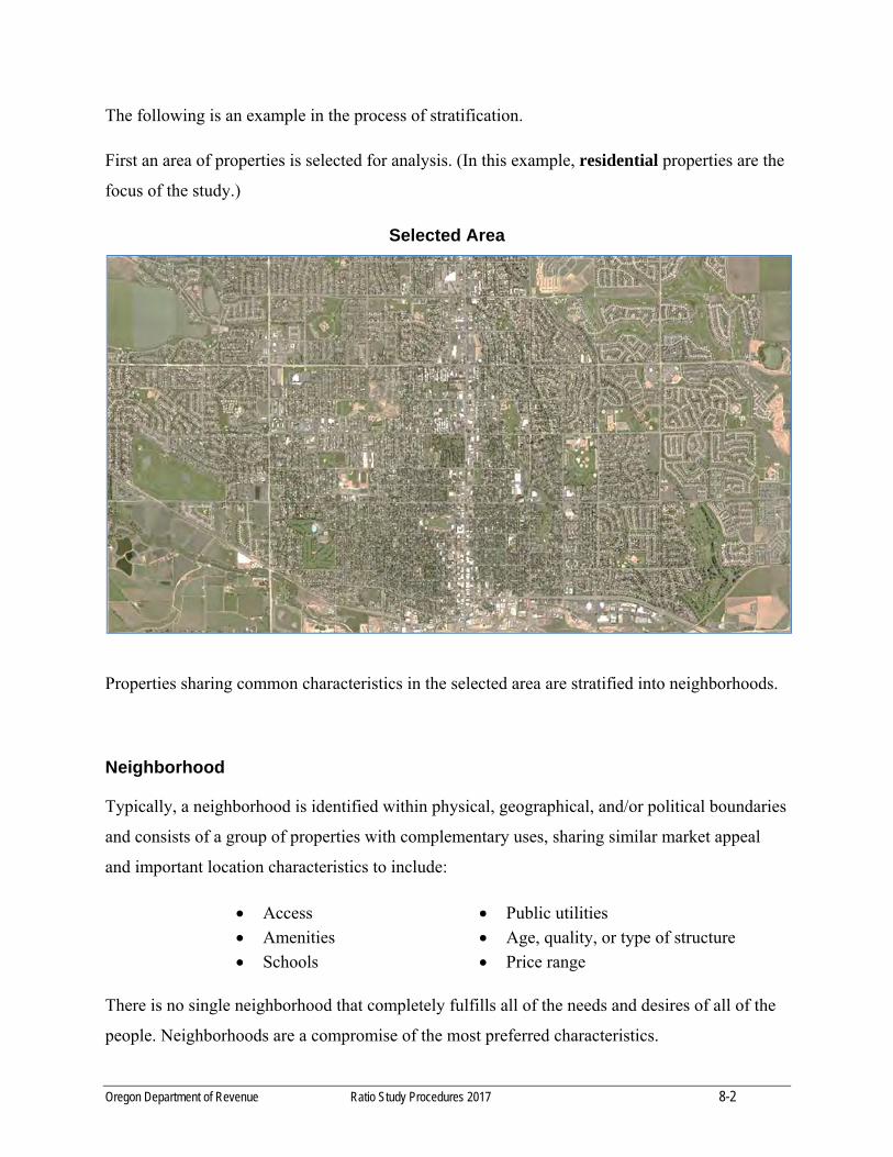
Oregon Department of Revenue Ratio Study Procedures 2017 8-2
The following is an example in the process of stratification.
First an area of properties is selected for analysis. (In this example, residential properties are the
focus of the study.)
Selected Area
Properties sharing common characteristics in the selected area are stratified into neighborhoods.
Neighborhood
Typically, a neighborhood is identified within physical, geographical, and/or political boundaries
and consists of a group of properties with complementary uses, sharing similar market appeal
and important location characteristics to include:
Access
Amenities
Schools
Public utilities
Age, quality, or type of structure
Price range There is no single neighborhood that completely fulfills all of the needs and desires of all of the
people. Neighborhoods are a compromise of the most preferred characteristics.
Oregon Department of Revenue Ratio Study Procedures 2015 8-3
Keep in mind the four factors of value when identifying neighborhoods: utility, scarcity, desire,
and effective purchasing power. Utility and scarcity by themselves do not make value. A
potential buyer must also have a desire and the financial means to complete the purchase.
Utility is the ability of a property to satisfy a human want or need.
Scarcity is created through the forces of supply and demand. As demand increases or supply decreases, the value of a property will likely change.
Desire is the potential purchaser’s wish to obtain an item.
Effective purchasing power means the ability to participate in the market with cash or its equivalency.
Some neighborhood components to consider are:
Amenities (quality of schools, parks, open spaces, recreational opportunities, proximity to public transportation)
Access (street patterns, road surface)
Public utilities (water, sewer/septic, internet, electric)
Land (size, shape, topography, view)
Structure (age, quality of construction, size)
Price range
Amenities, access, and public utilities are factors that generally contribute to desirability of
location and need to be documented. The other neighborhood components of land size, structural
characteristics, and price range are factors that can be numerically quantified and should be
utilized to further identify a contiguous group of compatible properties within a location.
Once the boundary of compatible properties is identified, a neighborhood can be created.
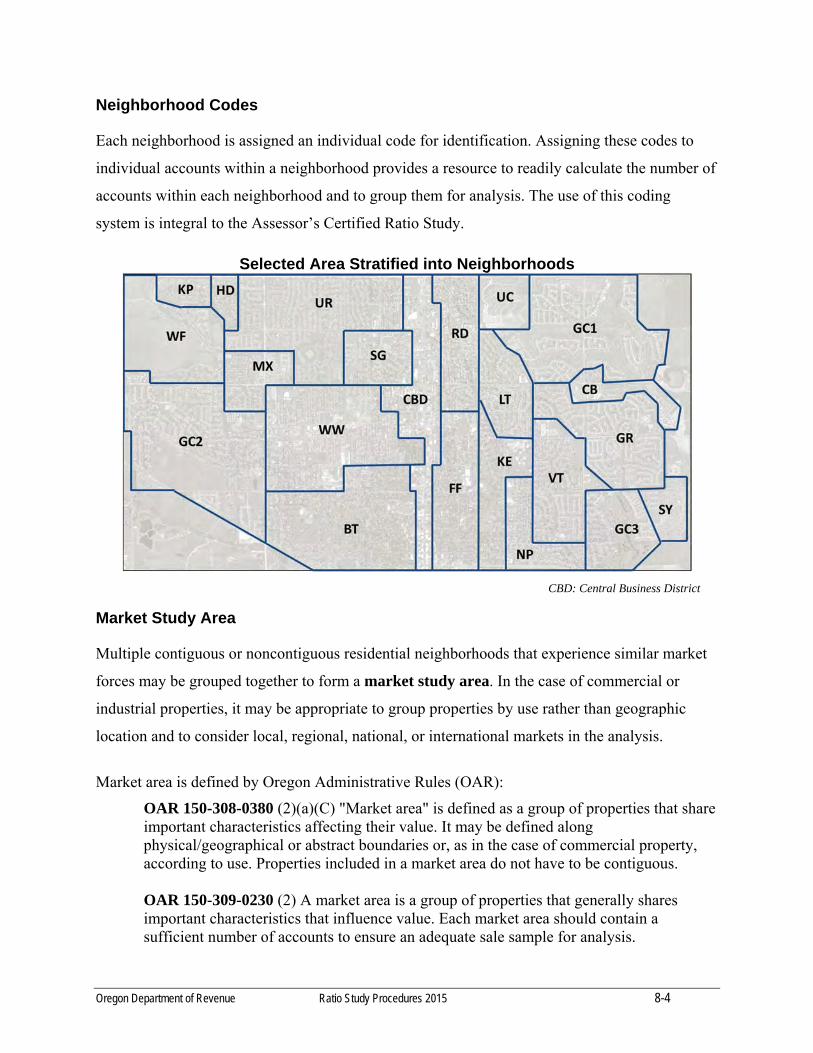
Oregon Department of Revenue Ratio Study Procedures 2015 8-4
Neighborhood Codes
Each neighborhood is assigned an individual code for identification. Assigning these codes to
individual accounts within a neighborhood provides a resource to readily calculate the number of
accounts within each neighborhood and to group them for analysis. The use of this coding
system is integral to the Assessor’s Certified Ratio Study.
Selected Area Stratified into Neighborhoods
CBD: Central Business District
Market Study Area
Multiple contiguous or noncontiguous residential neighborhoods that experience similar market
forces may be grouped together to form a market study area. In the case of commercial or
industrial properties, it may be appropriate to group properties by use rather than geographic
location and to consider local, regional, national, or international markets in the analysis.
Market area is defined by Oregon Administrative Rules (OAR):
OAR 150-308-0380 (2)(a)(C) "Market area" is defined as a group of properties that share important characteristics affecting their value. It may be defined along physical/geographical or abstract boundaries or, as in the case of commercial property, according to use. Properties included in a market area do not have to be contiguous. OAR 150-309-0230 (2) A market area is a group of properties that generally shares important characteristics that influence value. Each market area should contain a sufficient number of accounts to ensure an adequate sale sample for analysis.
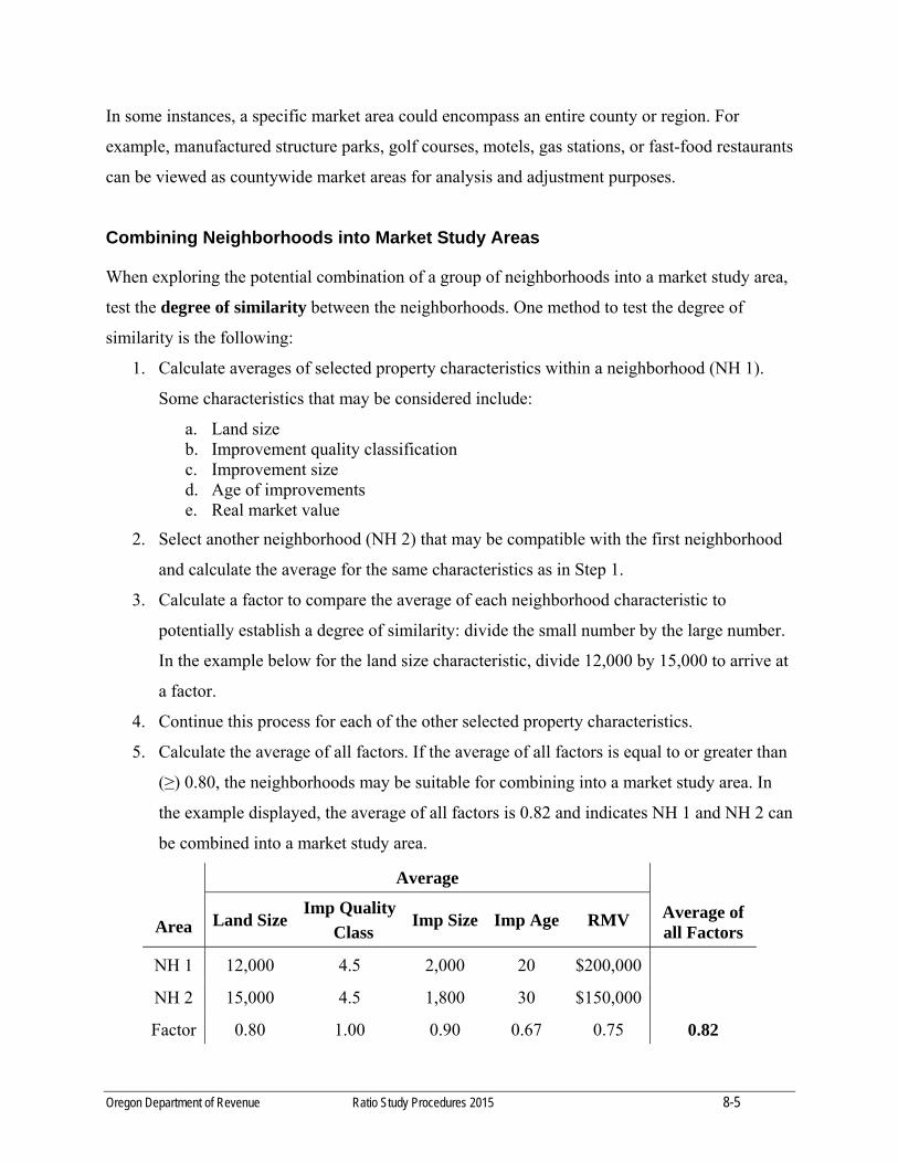
Oregon Department of Revenue Ratio Study Procedures 2015 8-5
In some instances, a specific market area could encompass an entire county or region. For
example, manufactured structure parks, golf courses, motels, gas stations, or fast-food restaurants
can be viewed as countywide market areas for analysis and adjustment purposes.
Combining Neighborhoods into Market Study Areas
When exploring the potential combination of a group of neighborhoods into a market study area,
test the degree of similarity between the neighborhoods. One method to test the degree of
similarity is the following:
1. Calculate averages of selected property characteristics within a neighborhood (NH 1).
Some characteristics that may be considered include:
a. Land size b. Improvement quality classification c. Improvement size d. Age of improvements e. Real market value
2. Select another neighborhood (NH 2) that may be compatible with the first neighborhood
and calculate the average for the same characteristics as in Step 1.
3. Calculate a factor to compare the average of each neighborhood characteristic to
potentially establish a degree of similarity: divide the small number by the large number.
In the example below for the land size characteristic, divide 12,000 by 15,000 to arrive at
a factor.
4. Continue this process for each of the other selected property characteristics.
5. Calculate the average of all factors. If the average of all factors is equal to or greater than
(≥) 0.80, the neighborhoods may be suitable for combining into a market study area. In
the example displayed, the average of all factors is 0.82 and indicates NH 1 and NH 2 can
be combined into a market study area.
Area
Average
Average of all Factors
Land Size Imp Quality
Class Imp Size Imp Age RMV
NH 1 12,000 4.5 2,000 20 $200,000
NH 2 15,000 4.5 1,800 30 $150,000
Factor 0.80 1.00 0.90 0.67 0.75 0.82
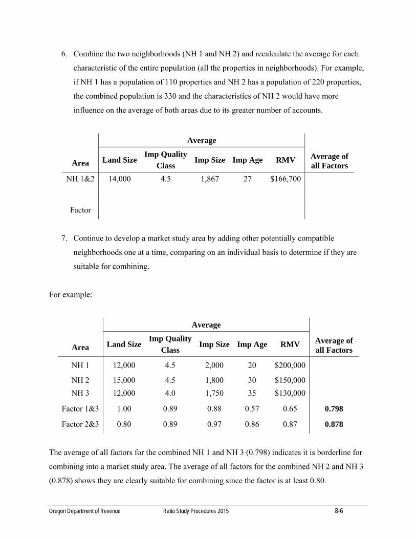
Oregon Department of Revenue Ratio Study Procedures 2015 8-6
6. Combine the two neighborhoods (NH 1 and NH 2) and recalculate the average for each
characteristic of the entire population (all the properties in neighborhoods). For example,
if NH 1 has a population of 110 properties and NH 2 has a population of 220 properties,
the combined population is 330 and the characteristics of NH 2 would have more
influence on the average of both areas due to its greater number of accounts.
Area
Average
Average of all Factors
Land Size Imp Quality
Class Imp Size Imp Age RMV
NH 1&2 14,000 4.5 1,867 27 $166,700
Factor
7. Continue to develop a market study area by adding other potentially compatible
neighborhoods one at a time, comparing on an individual basis to determine if they are
suitable for combining.
For example:
Area
Average
Average of all Factors
Land Size Imp Quality
Class Imp Size Imp Age RMV
NH 1 12,000 4.5 2,000 20 $200,000
NH 2 15,000 4.5 1,800 30 $150,000
NH 3 12,000 4.0 1,750 35 $130,000
Factor 1&3 1.00 0.89 0.88 0.57 0.65 0.798
Factor 2&3 0.80 0.89 0.97 0.86 0.87 0.878
The average of all factors for the combined NH 1 and NH 3 (0.798) indicates it is borderline for
combining into a market study area. The average of all factors for the combined NH 2 and NH 3
(0.878) shows they are clearly suitable for combining since the factor is at least 0.80.
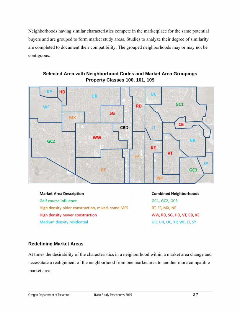
Oregon Department of Revenue Ratio Study Procedures 2015 8-7
Neighborhoods having similar characteristics compete in the marketplace for the same potential
buyers and are grouped to form market study areas. Studies to analyze their degree of similarity
are completed to document their compatibility. The grouped neighborhoods may or may not be
contiguous.
Selected Area with Neighborhood Codes and Market Area Groupings
Property Classes 100, 101, 109
Redefining Market Areas
At times the desirability of the characteristics in a neighborhood within a market area change and
necessitate a realignment of the neighborhood from one market area to another more compatible
market area.
Oregon Department of Revenue Ratio Study Procedures 2015 8-8
For example, a group of small towns countywide with similar characteristics are combined into a
single market study area. One town changed due to the development of a nearby resort and is
experiencing rapid growth. Analysis suggests it is no longer compatible with the other small
towns in the market study area. This town should be removed from the current market study area
and either studied as a separate market or combined with other compatible resort towns
experiencing similar economic conditions. This realignment benefits both market study areas. It
allows a focused analysis of the affected small town and avoids skewing the other small town
property RMVs not experiencing the new resort influence.
Reorganizing neighborhoods into different study areas should only be done when analysis
indicates a change is warranted. Calculation of the degree of similarity between a neighborhood
and the remainder of the market area can be used to document the need for modification.
Changes to market area composition must be documented in the ratio study report and the
appropriate analysis attached for review.
Conclusion
Stratification of properties into neighborhoods and then grouping neighborhoods into market
study areas is important for credible statistical analysis of market trends and the confident
development and application of annual value adjustments. Unsupported reorganization of
neighborhoods between market areas tends to undermine the integrity of the adjustment program.
Oregon Department of Revenue Ratio Study Procedures 2017 9-1
SECTION 9
ANALYZING DATA FOR SAMPLE BIAS,
MEASURES OF UNIFORMITY & RELIABILITY
Sample
Statistical techniques require samples (a set of observations selected from a population) to be
selected in a random manner. Random means that each member of a population has the same
chance of being selected as any other member.
Utilizing only sold properties may not represent a random sample because property owners are
not randomly chosen to sell their properties. Recognize that ratio studies may display bias
because the sample represents only sold properties.
Sample Bias
Bias is a systematic error that can prejudice findings in some way. It may be due to some flaw in
measurement or method. Bias due to method of sampling may arise when certain characteristics
are given a greater or lesser representation in the sample than in the population.
A ratio study by its nature may result in a biased sample simply because it is comprised of only
properties that recently sold and may not be representative of all properties in the market study
area. Ratio studies rely on a self-selection process that separates sold properties from those that
are unsold.
Example: A study area is in a town that consists of newer homes on in-fill lots mixed with older
homes of varying quality. Most of the sales are newer, average quality houses. The
sales of only newer houses biased this sample as they are not representative of the
older houses in the study area. Additional analysis may be necessary to determine if
the newer and older homes should be in separate study areas.
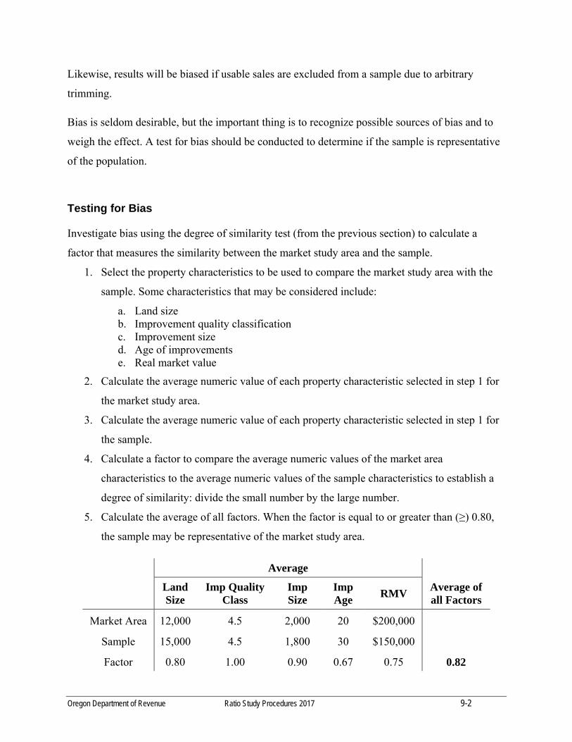
Oregon Department of Revenue Ratio Study Procedures 2017 9-2
Likewise, results will be biased if usable sales are excluded from a sample due to arbitrary
trimming.
Bias is seldom desirable, but the important thing is to recognize possible sources of bias and to
weigh the effect. A test for bias should be conducted to determine if the sample is representative
of the population.
Testing for Bias
Investigate bias using the degree of similarity test (from the previous section) to calculate a
factor that measures the similarity between the market study area and the sample.
1. Select the property characteristics to be used to compare the market study area with the
sample. Some characteristics that may be considered include:
a. Land size b. Improvement quality classification c. Improvement size d. Age of improvements e. Real market value
2. Calculate the average numeric value of each property characteristic selected in step 1 for
the market study area.
3. Calculate the average numeric value of each property characteristic selected in step 1 for
the sample.
4. Calculate a factor to compare the average numeric values of the market area
characteristics to the average numeric values of the sample characteristics to establish a
degree of similarity: divide the small number by the large number.
5. Calculate the average of all factors. When the factor is equal to or greater than (≥) 0.80,
the sample may be representative of the market study area.
Average
Average of all Factors
Land Size
Imp Quality Class
Imp Size
Imp Age
RMV
Market Area 12,000 4.5 2,000 20 $200,000
Sample 15,000 4.5 1,800 30 $150,000
Factor 0.80 1.00 0.90 0.67 0.75 0.82
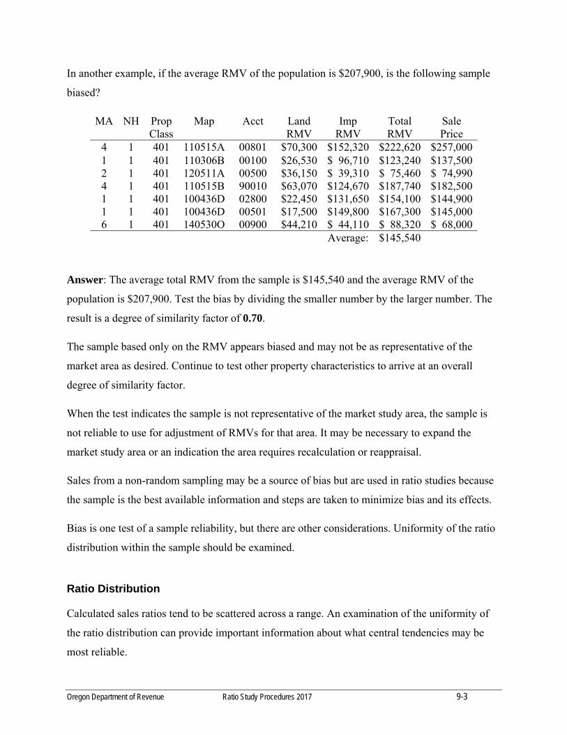
Oregon Department of Revenue Ratio Study Procedures 2017 9-3
In another example, if the average RMV of the population is $207,900, is the following sample
biased?
MA NH Prop Class
Map Acct Land RMV
Imp RMV
Total RMV
Sale Price
4 1 401 110515A 00801 $70,300 $152,320 $222,620 $257,0001 1 401 110306B 00100 $26,530 $ 96,710 $123,240 $137,5002 1 401 120511A 00500 $36,150 $ 39,310 $ 75,460 $ 74,9904 1 401 110515B 90010 $63,070 $124,670 $187,740 $182,5001 1 401 100436D 02800 $22,450 $131,650 $154,100 $144,9001 1 401 100436D 00501 $17,500 $149,800 $167,300 $145,0006 1 401 140530O 00900 $44,210 $ 44,110 $ 88,320 $ 68,000 Average: $145,540
Answer: The average total RMV from the sample is $145,540 and the average RMV of the
population is $207,900. Test the bias by dividing the smaller number by the larger number. The
result is a degree of similarity factor of 0.70.
The sample based only on the RMV appears biased and may not be as representative of the
market area as desired. Continue to test other property characteristics to arrive at an overall
degree of similarity factor.
When the test indicates the sample is not representative of the market study area, the sample is
not reliable to use for adjustment of RMVs for that area. It may be necessary to expand the
market study area or an indication the area requires recalculation or reappraisal.
Sales from a non-random sampling may be a source of bias but are used in ratio studies because
the sample is the best available information and steps are taken to minimize bias and its effects.
Bias is one test of a sample reliability, but there are other considerations. Uniformity of the ratio
distribution within the sample should be examined.
Ratio Distribution
Calculated sales ratios tend to be scattered across a range. An examination of the uniformity of
the ratio distribution can provide important information about what central tendencies may be
most reliable.
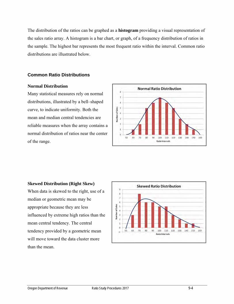
Oregon Department of Revenue Ratio Study Procedures 2017 9-4
The distribution of the ratios can be graphed as a histogram providing a visual representation of
the sales ratio array. A histogram is a bar chart, or graph, of a frequency distribution of ratios in
the sample. The highest bar represents the most frequent ratio within the interval. Common ratio
distributions are illustrated below.
Common Ratio Distributions Normal Distribution
Many statistical measures rely on normal
distributions, illustrated by a bell–shaped
curve, to indicate uniformity. Both the
mean and median central tendencies are
reliable measures when the array contains a
normal distribution of ratios near the center
of the range.
Skewed Distribution (Right Skew)
When data is skewed to the right, use of a
median or geometric mean may be
appropriate because they are less
influenced by extreme high ratios than the
mean central tendency. The central
tendency provided by a geometric mean
will move toward the data cluster more
than the mean.

Oregon Department of Revenue Ratio Study Procedures 2017 9-5
Skewed Distribution (Left Skew)
When data is skewed to the left, the median
is the most appropriate measure. The
central tendency provided by a geometric
mean will move away from the data cluster
more than the mean or median and is a less
reliable measure.
Bimodal Distribution
When there is more than one curve, the
sales array may indicate there is a need to
further stratify the sales data into two or
more groups, i.e., different ages or classes
of houses, lot sizes, amenities as view/non-
view, etc. for additional analyses.
Since the sales array is a representation of the total population or market area, multiple market
influences can be occurring at the same time. By stratifying the original sales array further, a
more accurate picture is derived and adjustments can be applied more accurately to those
properties being affected provided there are sufficient sales.

Oregon Department of Revenue Ratio Study Procedures 2017 9-6
Construct a Histogram
Ratio distribution depicted in a histogram can provide important information about what central
tendencies may be most reliable. To construct a histogram that displays ratio frequency
distribution, array all the ratios from the market study area, select intervals in which to group the
ratios, and then count the number of ratios in each interval.
Example 1 Normal Distribution - Bell Curve
This histogram displays the number of times each ratio appears in the range of 59 to 140 showing
a normal distribution in a bell curve. The mean or median central tendencies would likely best
represent the market conditions in this study area.
Range: (45‐54) (55‐64) (65‐74) (75‐84) (85‐94) (95‐104) (105‐114) (115‐124) (125‐134) (135‐144) (145‐154)
Interval: 50 60 70 80 90 100 110 120 130 140 150
# Ratios: 0 1 1 3 6 6 2 1 1 1 0
96 Mean 14 AAD 94 Median 15 COD 94 Geometric Mean 19 STD Dev
20 COV
0 1 1
3
6 6
2
1 1 1 00
1
2
3
4
5
6
7
45‐54 55‐64 65‐74 75‐84 85‐94 95‐104 105‐114 115‐124 125‐134 135‐144 145‐154
Frequency of Ratios
Ratio Intervals
Sale Ratio 1 59 2 70 3 76 4 81 5 82 6 86 7 87 8 88 9 88 10 91 11 93 12 95 13 97 14 99 15 101 16 102 17 103 18 107 19 111 20 118 21 133 22 140
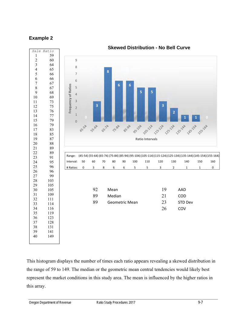
Oregon Department of Revenue Ratio Study Procedures 2017 9-7
Example 2
Skewed Distribution - No Bell Curve
92 Mean 19 AAD
89 Median 21 COD
89 Geometric Mean 23 STD Dev
26 COV
This histogram displays the number of times each ratio appears revealing a skewed distribution in
the range of 59 to 149. The median or the geometric mean central tendencies would likely best
represent the market conditions in this study area. The mean is influenced by the higher ratios in
this array.
0
3
8
6 6
5 5
3
2
1 1 00
1
2
3
4
5
6
7
8
9
Frequency of Ratios
Ratio Intervals
Range: (45‐54) (55‐64) (65‐74) (75‐84) (85‐94) (95‐104) (105‐114) (115‐124) (125‐134) (135‐144) (145‐154)(155‐164)
Interval: 50 60 70 80 90 100 110 120 130 140 150 160
# Ratios: 0 3 8 6 6 5 5 3 2 1 1 0
Sale Ratio 1 59 2 60 3 64 4 65 5 66 6 66 7 67 8 67 9 68 10 69 11 73 12 75 13 76 14 77 15 79 16 79 17 83 18 85 19 87 20 88 21 89 22 89 23 91 24 95 25 96 26 96 27 99 28 103 29 105 30 105 31 109 32 111 33 114 34 116 35 119 36 123 37 128 38 131 39 141 40 149
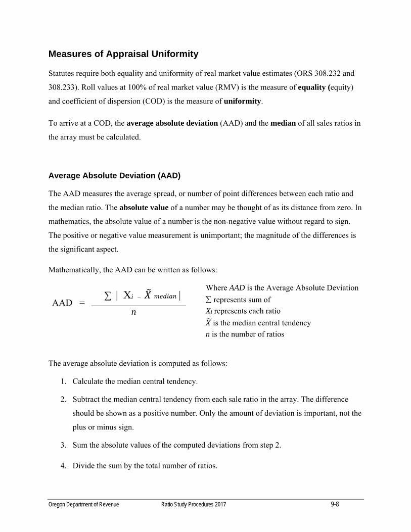
Oregon Department of Revenue Ratio Study Procedures 2017 9-8
Measures of Appraisal Uniformity
Statutes require both equality and uniformity of real market value estimates (ORS 308.232 and
308.233). Roll values at 100% of real market value (RMV) is the measure of equality (equity)
and coefficient of dispersion (COD) is the measure of uniformity.
To arrive at a COD, the average absolute deviation (AAD) and the median of all sales ratios in
the array must be calculated.
Average Absolute Deviation (AAD)
The AAD measures the average spread, or number of point differences between each ratio and
the median ratio. The absolute value of a number may be thought of as its distance from zero. In
mathematics, the absolute value of a number is the non-negative value without regard to sign.
The positive or negative value measurement is unimportant; the magnitude of the differences is
the significant aspect.
Mathematically, the AAD can be written as follows:
Where AAD is the Average Absolute Deviation
represents sum of
Xi represents each ratio
is the median central tendency
n is the number of ratios
The average absolute deviation is computed as follows:
1. Calculate the median central tendency.
2. Subtract the median central tendency from each sale ratio in the array. The difference
should be shown as a positive number. Only the amount of deviation is important, not the
plus or minus sign.
3. Sum the absolute values of the computed deviations from step 2.
4. Divide the sum by the total number of ratios.
AAD = ∑ | Xi - |
n
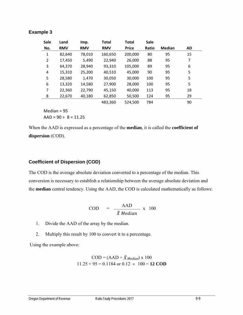
Oregon Department of Revenue Ratio Study Procedures 2017 9-9
Example 3
Sale Land Imp. Total Total Sale No. RMV RMV RMV Price Ratio Median AD
1 82,640 78,010 160,650 200,000 80 95 15
2 17,450 5,490 22,940 26,000 88 95 7
3 64,370 28,940 93,310 105,000 89 95 6
4 15,310 25,200 40,510 45,000 90 95 5
5 28,580 1,470 30,050 30,000 100 95 5
6 13,320 14,580 27,900 28,000 100 95 5
7 22,360 22,790 45,150 40,000 113 95 18
8 22,670 40,180 62,850 50,500 124 95 29
483,360 524,500 784 90
Median = 95 AAD = 90 ÷ 8 = 11.25
When the AAD is expressed as a percentage of the median, it is called the coefficient of
dispersion (COD).
Coefficient of Dispersion (COD)
The COD is the average absolute deviation converted to a percentage of the median. This
conversion is necessary to establish a relationship between the average absolute deviation and
the median central tendency. Using the AAD, the COD is calculated mathematically as follows:
COD = AAD
x 100
1. Divide the AAD of the array by the median.
2. Multiply this result by 100 to convert it to a percentage.
Using the example above:
COD = (AAD ÷ Median) x 100 11.25 ÷ 95 = 0.1184 or 0.12 100 = 12 COD

Oregon Department of Revenue Ratio Study Procedures 2017 9-10
This computation is important in measuring uniformity of RMV. The COD indicates how widely
the values in an array vary from the central tendency (the median). The lower the percentage of
deviation, the greater the uniformity within the property class or sample.
Allowable coefficients of dispersion vary by property class. In general, depending on property
types, CODs ranging from 10 to 20 indicate acceptable assessment levels. Care should be taken
to ensure that low coefficients are the result of good appraisal valuation practices and not sale
chasing or inappropriate trim methods.
Single family residences in generally non-homogeneous areas should have coefficients of 15 or less. In newer and fairly homogeneous areas, 10 or less
Commercial properties in rural areas should have coefficients of 20 or less, and in larger urban jurisdictions, 15 or less
Vacant land and improved rural properties should have coefficients of 20 or less
Manufactured structures should have coefficients of 25 or less
Multi-family properties should have coefficients of 12 or less
COD Standards
The following table is from the Oregon Administrative Rule (OAR 150-308-0380). It outlines
the maximum COD standards, by property class, established by assessors and the DOR to
measure the results of the counties’ valuation programs in Oregon:
Type of property Maximum (Property Class) COD Vacant Land (100, 400) 20 Real & Personal Manufactured Structures/Mobile Homes 25 Urban Residential (101) Homogeneous 10 Nonhomogeneous 15 Rural Improved (101, 401) 20 Apartments (701) 12 Other Income (201) Large Urban 15 Smaller Rural 20
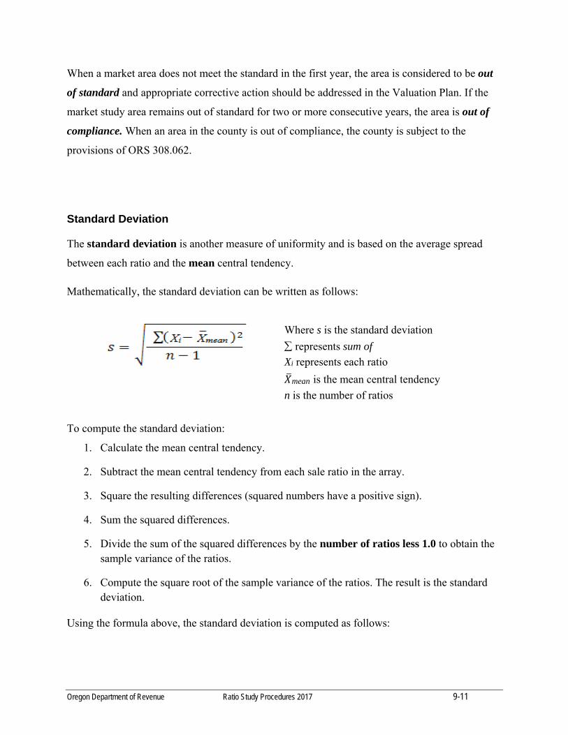
Oregon Department of Revenue Ratio Study Procedures 2017 9-11
When a market area does not meet the standard in the first year, the area is considered to be out
of standard and appropriate corrective action should be addressed in the Valuation Plan. If the
market study area remains out of standard for two or more consecutive years, the area is out of
compliance. When an area in the county is out of compliance, the county is subject to the
provisions of ORS 308.062.
Standard Deviation
The standard deviation is another measure of uniformity and is based on the average spread
between each ratio and the mean central tendency.
Mathematically, the standard deviation can be written as follows:
Where s is the standard deviation
represents sum of
Xi represents each ratio
mean is the mean central tendency
n is the number of ratios
To compute the standard deviation:
1. Calculate the mean central tendency.
2. Subtract the mean central tendency from each sale ratio in the array.
3. Square the resulting differences (squared numbers have a positive sign).
4. Sum the squared differences.
5. Divide the sum of the squared differences by the number of ratios less 1.0 to obtain the sample variance of the ratios.
6. Compute the square root of the sample variance of the ratios. The result is the standard deviation.
Using the formula above, the standard deviation is computed as follows:

Oregon Department of Revenue Ratio Study Procedures 2017 9-12
Example 4
Distribution of the Sample
The interpretation of the standard deviation needs to take into account whether the data can be
regarded as normally distributed. Normal distributions are seen as a symmetrical bell curve
when graphically represented. The definition of normal distribution implies the following:
1. 68 percent +/– of all sales fall within one standard deviation of the mean.
2. 95 percent +/– of all sales fall within two standard deviations of the mean.
3. 99 percent +/– of all sales fall within three standard deviations of the mean.
The following is a graphic illustration of the percentage of data that can be expected to occur
within each of three standard deviations from the mean in a normal distribution.
Sale Land Imp. Total Total Sale Squared
No. RMV RMV RMV Price Ratio Mean Difference Difference
1 82,640 78,010 160,650 200,000 80 98 ‐18 324
2 17,450 5,490 22,940 26,000 88 98 ‐10 100
3 64,370 28,940 93,310 105,000 89 98 ‐9 81
4 15,310 25,200 40,510 45,000 90 98 ‐8 64
5 28,580 1,470 30,050 30,000 100 98 2 4
6 13,320 14,580 27,900 28,000 100 98 2 4
7 22,360 22,790 45,150 40,000 113 98 15 225
8 22,670 40,180 62,850 50,500 124 98 26 676
483,360 524,500 784 1,478
Mean = 98
1,478 ÷ (8‐1) = 211 variance of ratios
Sq Root of 211 = 14.5 Standard Deviation = 14.5

Oregon Department of Revenue Ratio Study Procedures 2017 9-13
Example 5
If the sales array in Example 4 is normally distributed the results would be:
One standard deviation (14.5) on each side of the mean (98) will include approximately 68 percent of sales and the ratios between 83.5 and 112.5.
Two standard deviations (29) on each side of the mean (98) will include approximately 95 percent of sales and the ratios between 69 and 127.
Three standard deviations (43.5) on each side of the mean (98) will include approximately 99 percent of sales and the ratios between 54.5 and 141.5.
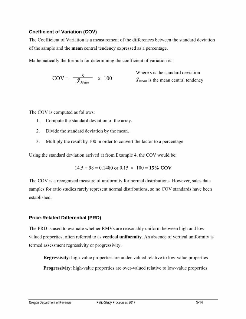
Oregon Department of Revenue Ratio Study Procedures 2017 9-14
Coefficient of Variation (COV)
The Coefficient of Variation is a measurement of the differences between the standard deviation
of the sample and the mean central tendency expressed as a percentage.
Mathematically the formula for determining the coefficient of variation is:
Where s is the standard deviation
mean is the mean central tendency
The COV is computed as follows:
1. Compute the standard deviation of the array.
2. Divide the standard deviation by the mean.
3. Multiply the result by 100 in order to convert the factor to a percentage.
Using the standard deviation arrived at from Example 4, the COV would be:
14.5 ÷ 98 = 0.1480 or 0.15 100 = 15% COV
The COV is a recognized measure of uniformity for normal distributions. However, sales data
samples for ratio studies rarely represent normal distributions, so no COV standards have been
established.
Price-Related Differential (PRD)
The PRD is used to evaluate whether RMVs are reasonably uniform between high and low
valued properties, often referred to as vertical uniformity. An absence of vertical uniformity is
termed assessment regressivity or progressivity.
Regressivity: high-value properties are under-valued relative to low-value properties
Progressivity: high-value properties are over-valued relative to low-value properties
COV = s x 100Mean
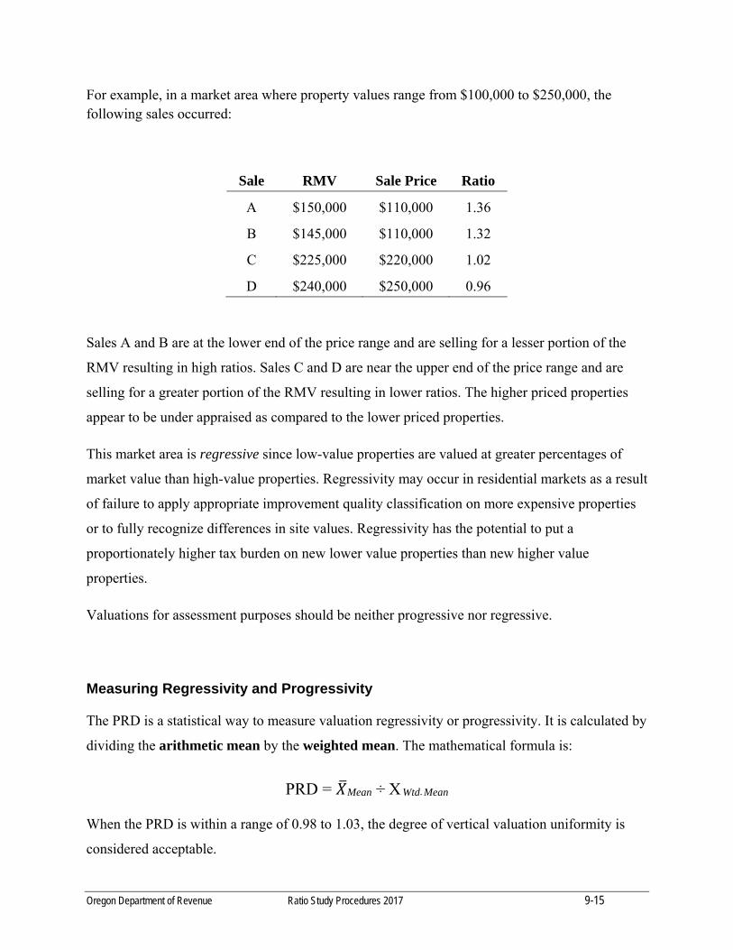
Oregon Department of Revenue Ratio Study Procedures 2017 9-15
For example, in a market area where property values range from $100,000 to $250,000, the following sales occurred:
Sale RMV Sale Price Ratio
A $150,000 $110,000 1.36
B $145,000 $110,000 1.32
C $225,000 $220,000 1.02
D $240,000 $250,000 0.96
Sales A and B are at the lower end of the price range and are selling for a lesser portion of the
RMV resulting in high ratios. Sales C and D are near the upper end of the price range and are
selling for a greater portion of the RMV resulting in lower ratios. The higher priced properties
appear to be under appraised as compared to the lower priced properties.
This market area is regressive since low-value properties are valued at greater percentages of
market value than high-value properties. Regressivity may occur in residential markets as a result
of failure to apply appropriate improvement quality classification on more expensive properties
or to fully recognize differences in site values. Regressivity has the potential to put a
proportionately higher tax burden on new lower value properties than new higher value
properties.
Valuations for assessment purposes should be neither progressive nor regressive.
Measuring Regressivity and Progressivity
The PRD is a statistical way to measure valuation regressivity or progressivity. It is calculated by
dividing the arithmetic mean by the weighted mean. The mathematical formula is:
PRD = Mean ÷ X Wtd. Mean
When the PRD is within a range of 0.98 to 1.03, the degree of vertical valuation uniformity is
considered acceptable.
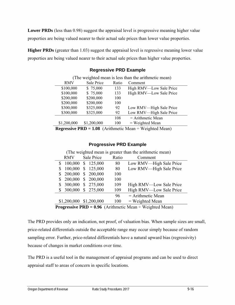
Oregon Department of Revenue Ratio Study Procedures 2017 9-16
Lower PRDs (less than 0.98) suggest the appraisal level is progressive meaning higher value
properties are being valued nearer to their actual sale prices than lower value properties.
Higher PRDs (greater than 1.03) suggest the appraisal level is regressive meaning lower value
properties are being valued nearer to their actual sale prices than higher value properties.
Regressive PRD Example
(The weighted mean is less than the arithmetic mean) RMV Sale Price Ratio Comment $100,000 $ 75,000 133 High RMV—Low Sale Price $100,000 $ 75,000 133 High RMV—Low Sale Price $200,000 $200,000 100 $200,000 $200,000 100 $300,000 $325,000 92 Low RMV—High Sale Price $300,000 $325,000 92 Low RMV—High Sale Price 108 = Arithmetic Mean
$1,200,000 $1,200,000 100 = Weighted Mean Regressive PRD = 1.08 (Arithmetic Mean ÷ Weighted Mean)
Progressive PRD Example
(The weighted mean is greater than the arithmetic mean) RMV Sale Price Ratio Comment $ 100,000 $ 125,000 80 Low RMV—High Sale Price $ 100,000 $ 125,000 80 Low RMV—High Sale Price $ 200,000 $ 200,000 100 $ 200,000 $ 200,000 100 $ 300,000 $ 275,000 109 High RMV—Low Sale Price $ 300,000 $ 275,000 109 High RMV—Low Sale Price 96 = Arithmetic Mean $1,200,000 $1,200,000 100 = Weighted Mean Progressive PRD = 0.96 (Arithmetic Mean ÷ Weighted Mean)
The PRD provides only an indication, not proof, of valuation bias. When sample sizes are small,
price-related differentials outside the acceptable range may occur simply because of random
sampling error. Further, price-related differentials have a natural upward bias (regressivity)
because of changes in market conditions over time.
The PRD is a useful tool in the management of appraisal programs and can be used to direct
appraisal staff to areas of concern in specific locations.
Oregon Department of Revenue Ratio Study Procedures 2017 9-17
Weighting
Weighting is a process that maintains land value uniformity between vacant land accounts and
the land component of improved accounts. The ultimate goal in the weighting process is to
distribute the overall adjustment in proper proportions among the components of value (land,
onsite development, primary improvements, and farm buildings) in a market area.
A land adjustment factor is calculated through a study of vacant land sales. An overall market
area adjustment is calculated for improved properties. The land adjustment factor is applied to
the land component of improved properties. The weighting process provides a basis for
calculation of the adjustment factor to be applied to the improvement component to achieve the
overall adjustment.
Elements needed to compute an unknown adjustment factor for a study area:
• RMV of the components (land, OSD, improvements, farm buildings);
• The overall adjustment factor computed from the selected central tendency;
• Known adjustment factors for all components from other studies (except for the one
unknown factor).
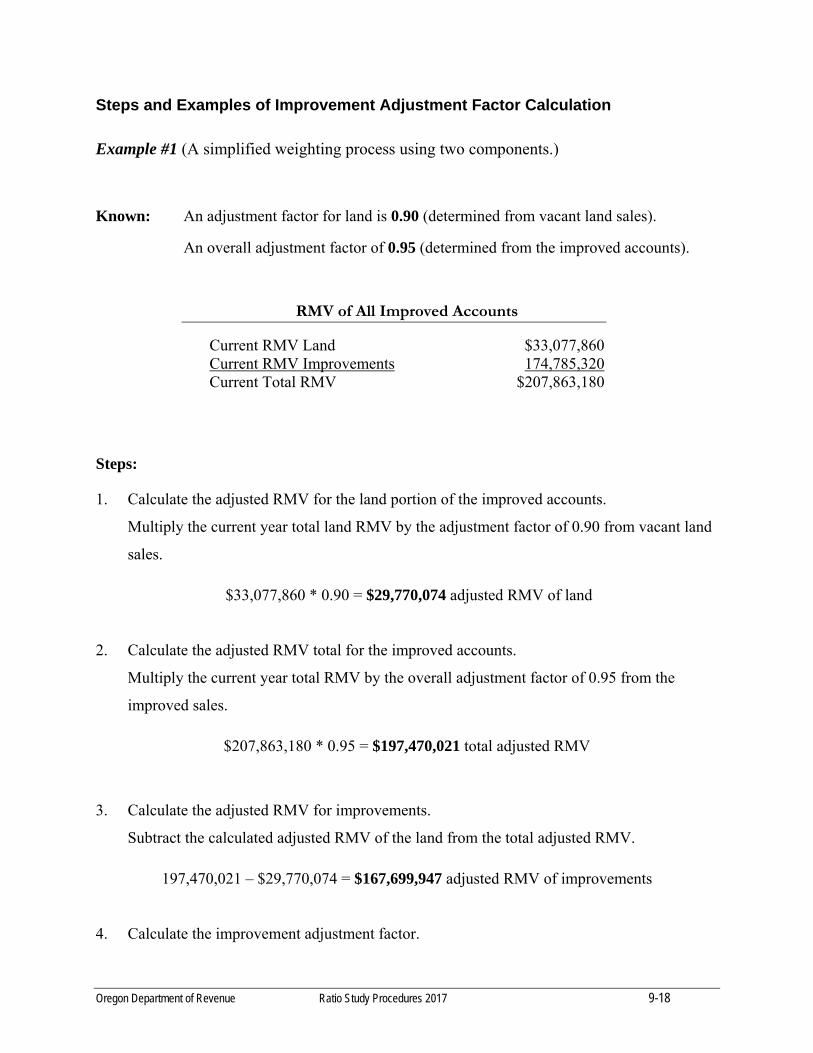
Oregon Department of Revenue Ratio Study Procedures 2017 9-18
Steps and Examples of Improvement Adjustment Factor Calculation
Example #1 (A simplified weighting process using two components.)
Known: An adjustment factor for land is 0.90 (determined from vacant land sales).
An overall adjustment factor of 0.95 (determined from the improved accounts).
RMV of All Improved Accounts
Current RMV Land $33,077,860 Current RMV Improvements 174,785,320 Current Total RMV $207,863,180
Steps:
1. Calculate the adjusted RMV for the land portion of the improved accounts.
Multiply the current year total land RMV by the adjustment factor of 0.90 from vacant land
sales.
$33,077,860 * 0.90 = $29,770,074 adjusted RMV of land
2. Calculate the adjusted RMV total for the improved accounts.
Multiply the current year total RMV by the overall adjustment factor of 0.95 from the
improved sales.
$207,863,180 * 0.95 = $197,470,021 total adjusted RMV
3. Calculate the adjusted RMV for improvements.
Subtract the calculated adjusted RMV of the land from the total adjusted RMV.
197,470,021 – $29,770,074 = $167,699,947 adjusted RMV of improvements
4. Calculate the improvement adjustment factor.
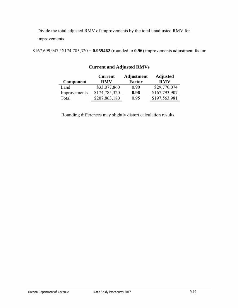
Oregon Department of Revenue Ratio Study Procedures 2017 9-19
Divide the total adjusted RMV of improvements by the total unadjusted RMV for
improvements.
$167,699,947 / $174,785,320 = 0.959462 (rounded to 0.96) improvements adjustment factor
Current and Adjusted RMVs
Component Current
RMV Adjustment
Factor Adjusted
RMV Land $33,077,860 0.90 $29,770,074 Improvements $174,785,320 0.96 $167,793,907 Total $207,863,180 0.95 $197,563,981
Rounding differences may slightly distort calculation results.
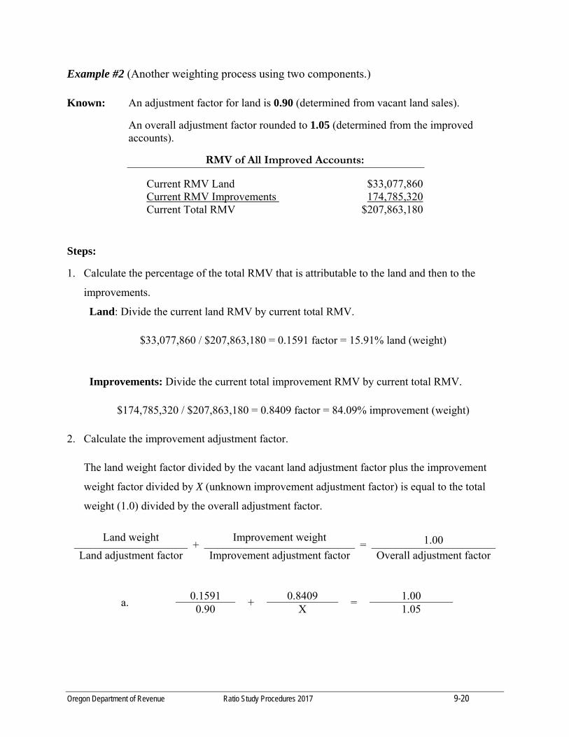
Oregon Department of Revenue Ratio Study Procedures 2017 9-20
Example #2 (Another weighting process using two components.)
Known: An adjustment factor for land is 0.90 (determined from vacant land sales).
An overall adjustment factor rounded to 1.05 (determined from the improved accounts).
RMV of All Improved Accounts:
Current RMV Land $33,077,860 Current RMV Improvements 174,785,320 Current Total RMV $207,863,180
Steps:
1. Calculate the percentage of the total RMV that is attributable to the land and then to the
improvements.
Land: Divide the current land RMV by current total RMV.
$33,077,860 / $207,863,180 = 0.1591 factor = 15.91% land (weight)
Improvements: Divide the current total improvement RMV by current total RMV.
$174,785,320 / $207,863,180 = 0.8409 factor = 84.09% improvement (weight)
2. Calculate the improvement adjustment factor.
The land weight factor divided by the vacant land adjustment factor plus the improvement
weight factor divided by X (unknown improvement adjustment factor) is equal to the total
weight (1.0) divided by the overall adjustment factor.
Land weight +
Improvement weight = 1.00
Land adjustment factor Improvement adjustment factor Overall adjustment factor
a. 0.1591
+ 0.8409
= 1.00
0.90 X 1.05
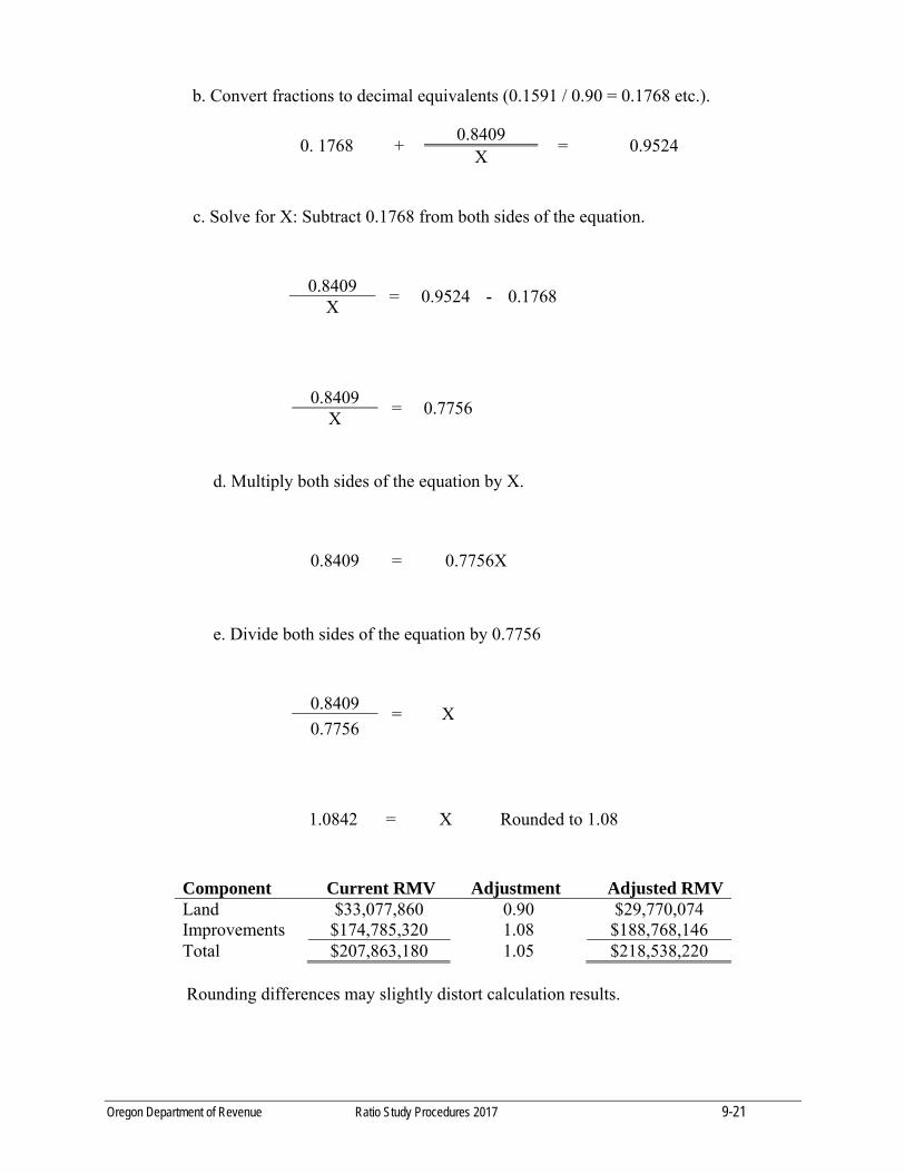
Oregon Department of Revenue Ratio Study Procedures 2017 9-21
c. Solve for X: Subtract 0.1768 from both sides of the equation.
d. Multiply both sides of the equation by X.
e. Divide both sides of the equation by 0.7756
Component Current RMV Adjustment Adjusted RMV Land $33,077,860 0.90 $29,770,074 Improvements $174,785,320 1.08 $188,768,146 Total $207,863,180 1.05 $218,538,220
Rounding differences may slightly distort calculation results.
b. Convert fractions to decimal equivalents (0.1591 / 0.90 = 0.1768 etc.).
0. 1768 + 0.8409
= 0.9524 X
0.8409 = 0.9524 - 0.1768
X
0.8409 = 0.7756
X
0.8409 = 0.7756X
0.8409 = X
0.7756
1.0842 = X Rounded to 1.08
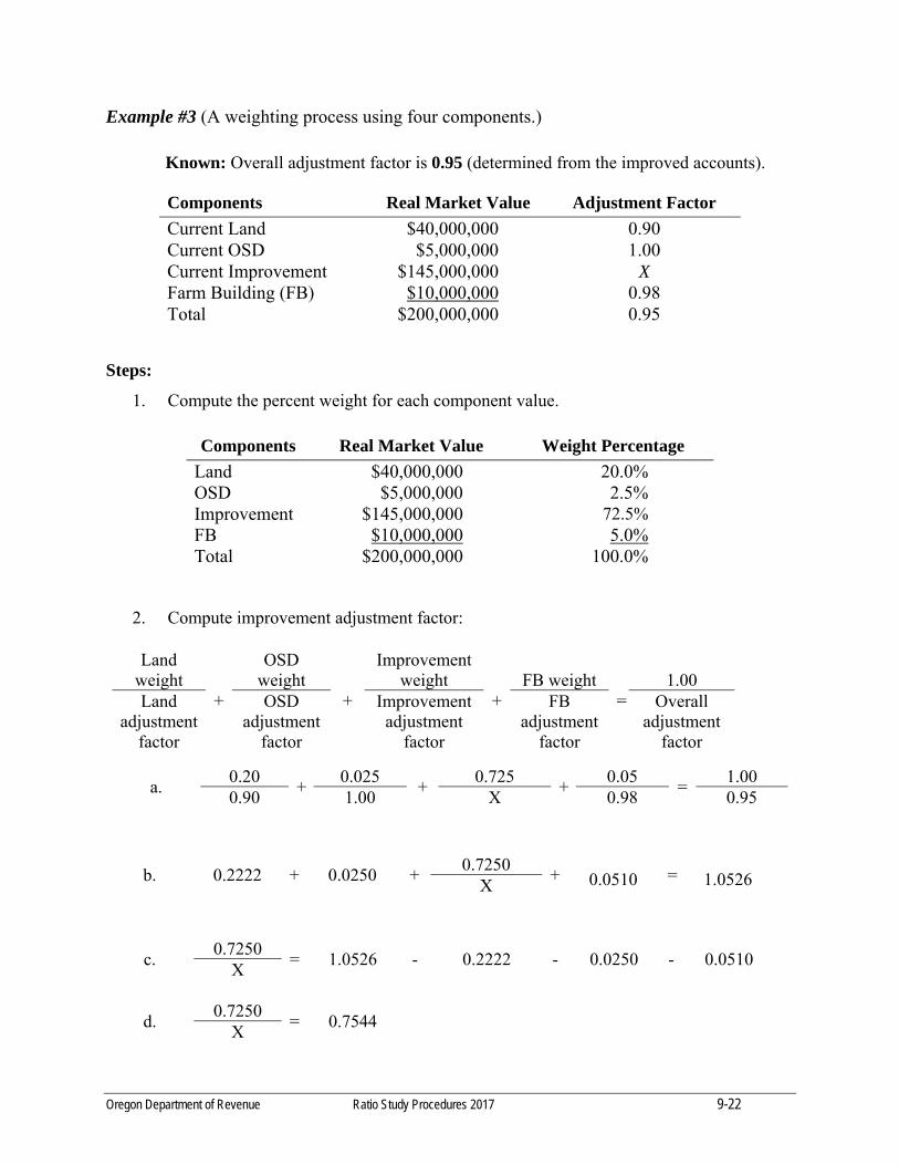
Oregon Department of Revenue Ratio Study Procedures 2017 9-22
Example #3 (A weighting process using four components.)
Known: Overall adjustment factor is 0.95 (determined from the improved accounts).
Components Real Market Value Adjustment Factor
Current Land $40,000,000 0.90 Current OSD $5,000,000 1.00 Current Improvement $145,000,000 X Farm Building (FB) $10,000,000 0.98 Total $200,000,000 0.95
Steps:
1. Compute the percent weight for each component value.
Components Real Market Value Weight Percentage
Land $40,000,000 20.0% OSD $5,000,000 2.5% Improvement $145,000,000 72.5% FB $10,000,000 5.0% Total $200,000,000 100.0%
2. Compute improvement adjustment factor:
Land weight
+
OSD weight
+
Improvement weight
+FB weight
=1.00
Land adjustment
factor
OSD adjustment
factor
Improvement adjustment
factor
FB adjustment
factor
Overall adjustment
factor
a. 0.20
+ 0.025
+ 0.725
+0.05
= 1.00
0.90 1.00 X 0.98 0.95
b. 0.2222 + 0.0250 + 0.7250
+ 0.0510 = 1.0526 X
c. 0.7250
= 1.0526 - 0.2222 - 0.0250 - 0.0510 X
d. 0.7250
= 0.7544 X

Oregon Department of Revenue Ratio Study Procedures 2017 9-23
e. Multiply both sides of the equation by X.
0.7250 = 0.7544X
f. Divide both sides of the equation by 0.7544.
0.96 = X
Components Current RMV
Adjustment Adjusted RMV
Land $40,000,000 0.90 $36,000,000 OSD $5,000,000 1.00 $5,000,000 Improvement $145,000,000 0.96 $139,200,000 FB $10,000,000 0.98 $9,800,000 Total $200,000,000 0.95 $190,000,000
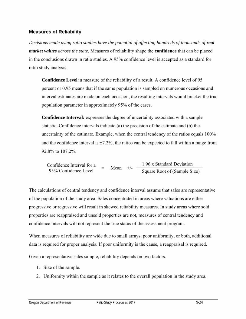
Oregon Department of Revenue Ratio Study Procedures 2017 9-24
Measures of Reliability
Decisions made using ratio studies have the potential of affecting hundreds of thousands of real
market values across the state. Measures of reliability shape the confidence that can be placed
in the conclusions drawn in ratio studies. A 95% confidence level is accepted as a standard for
ratio study analysis.
Confidence Level: a measure of the reliability of a result. A confidence level of 95
percent or 0.95 means that if the same population is sampled on numerous occasions and
interval estimates are made on each occasion, the resulting intervals would bracket the true
population parameter in approximately 95% of the cases.
Confidence Interval: expresses the degree of uncertainty associated with a sample
statistic. Confidence intervals indicate (a) the precision of the estimate and (b) the
uncertainty of the estimate. Example, when the central tendency of the ratios equals 100%
and the confidence interval is 7.2%, the ratios can be expected to fall within a range from
92.8% to 107.2%.
Confidence Interval for a 95% Confidence Level
= Mean +/- 1.96 x Standard Deviation
Square Root of (Sample Size)
The calculations of central tendency and confidence interval assume that sales are representative
of the population of the study area. Sales concentrated in areas where valuations are either
progressive or regressive will result in skewed reliability measures. In study areas where sold
properties are reappraised and unsold properties are not, measures of central tendency and
confidence intervals will not represent the true status of the assessment program.
When measures of reliability are wide due to small arrays, poor uniformity, or both, additional
data is required for proper analysis. If poor uniformity is the cause, a reappraisal is required.
Given a representative sales sample, reliability depends on two factors.
1. Size of the sample.
2. Uniformity within the sample as it relates to the overall population in the study area.
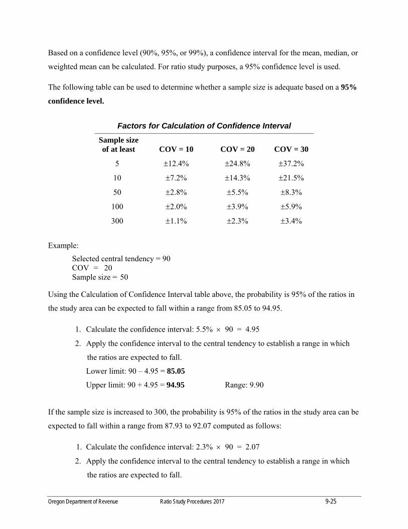
Oregon Department of Revenue Ratio Study Procedures 2017 9-25
Based on a confidence level (90%, 95%, or 99%), a confidence interval for the mean, median, or
weighted mean can be calculated. For ratio study purposes, a 95% confidence level is used.
The following table can be used to determine whether a sample size is adequate based on a 95%
confidence level.
Factors for Calculation of Confidence Interval
Sample size of at least COV = 10 COV = 20 COV = 30
5 12.4% 24.8% 37.2%
10 7.2% 14.3% 21.5%
50 2.8% 5.5% 8.3%
100 2.0% 3.9% 5.9%
300 1.1% 2.3% 3.4%
Example:
Selected central tendency = 90 COV = 20 Sample size = 50
Using the Calculation of Confidence Interval table above, the probability is 95% of the ratios in
the study area can be expected to fall within a range from 85.05 to 94.95.
1. Calculate the confidence interval: 5.5% 90 = 4.95
2. Apply the confidence interval to the central tendency to establish a range in which
the ratios are expected to fall.
Lower limit: 90 – 4.95 = 85.05
Upper limit: 90 + 4.95 = 94.95 Range: 9.90
If the sample size is increased to 300, the probability is 95% of the ratios in the study area can be
expected to fall within a range from 87.93 to 92.07 computed as follows:
1. Calculate the confidence interval: 2.3% 90 = 2.07
2. Apply the confidence interval to the central tendency to establish a range in which
the ratios are expected to fall.

Oregon Department of Revenue Ratio Study Procedures 2017 9-26
Lower limit: 90 – 2.07 = 87.93
Upper limit: 90 + 2.07 = 92.07 Range: 4.14
In the second example, by adjusting only the sample size, there is a greater confidence in the
interval results reflecting increased reliability of the sample. This is demonstrated by the reduced
range between the ratios in the second example, 4.14 compared to the first example 9.90.
This next example demonstrates the selected central tendency of 93 is not a supportable market
indication because of the 46.12 confidence interval range.
Example:
Selected central tendency = 93 COV = 24 Sample size = 6
Using the Calculation of Confidence Interval table above, the probability is 95% of the ratios in
the study area can be expected to fall within a range from 69.94 to 116.06.
1. Calculate the confidence interval: 24.8% 93 = 23.06
2. Apply the confidence interval to the central tendency to establish a range in which
the ratios are expected to fall.
Lower limit: 93 – 23.06 = 69.94
Upper limit: 93 + 23.06 = 116.06 Range: 46.12
IAAO Standard on Ratio Studies 2013, page 34 11.1.2 Recommended Appraisal Level Standards for Direct and Indirect Equalization The performance standard adopted by an oversight agency should be a range around the legally required level of appraisal in a property class or an overall jurisdiction. This range should be 90 to 110 percent of the legally required level of appraisal for direct equalization or reappraisal, or 95 to 105 percent for indirect equalization. A smaller maximum range for indirect equalization is justified because taxpayers are not as comprehensively affected. Oversight agencies should adopt performance standards that are as close to the legally required level as can be justified given the local situation and taking into account the factors discussed herein. In addition to the above appraisal level standards, each class of property for which appraisal level standards have been defined must be within 5 percent of the overall level of appraisal of the jurisdiction (see section 11.2.3, “Uniformity among Strata,” in this part). Both criteria must be met.
Oregon Department of Revenue Ratio Study Procedures 2017 10-1
SECTION 10
RECALCULATION TRENDING
AND ADDITIONAL STUDIES
Recalculation
Traditional trending in Oregon began in the 1970s as a method of testing and adjusting true cash
values of properties in the time period between six-year appraisal cycles. The trends were based
on sales studies of market movement over time in each cycle maintenance area and applied
annually. As time passed, the studies became more detailed where land and improvements were
studied and trended separately within each maintenance area. Eventually, traditional trending
was refined to separate the value contributions of land, on site development (OSD), major
improvements, and farm buildings within market study areas.
Recalculation further refines the process and is essentially a more comprehensive form of
trending. An existing valuation model is adjusted or a new one created based on current market
analysis of property characteristics. Application of the modified model calculates a new estimate
of real market value for each property.
It is important to compare the traditional trending, the recalculation process, and appraisal:
Traditional trending, recalculation, and appraisal all calculate new market values
estimates
Both recalculation and appraisal rely on constructing valuation models based on current
market analysis
Recalculation relies on the inventory characteristics as they appear on the assessment
record without field verification of the characteristics of the unsold properties in the
market study area
Appraisal requires field verification and updating of property characteristics through
physical inspections of all properties being revalued to assure equal and equitable
treatment of both sold and unsold properties
Oregon Department of Revenue Ratio Study Procedures 2017 10-2
Values developed through recalculation are treated differently than those developed through
reappraisal when applied to adjudicated RMVs. By statute, when an area is trended, adjudicated
values can be adjusted to proportionately reflect the percentage change in value due to the
adjudication. However, when a property is reappraised, the adjudicated values may not be
changed.
Oregon Revised Statute 309.115 and the associated OAR 150-309-0210(3) provide direction and
clarification for adjustment of adjudicated values.
ORS 309.115 Effect of property value correction upon appeal; exceptions. (1) If the Department of Revenue, the board of property tax appeals or the tax court or other court enters an order correcting the real market value of a separate assessment of property and there is no further appeal from that order, except as provided under subsection (2) or (3) of this section, the value so entered shall be the real market value entered on the assessment and tax rolls for the five assessment years next following the year for which the order is entered. (2) Notwithstanding subsection (1) of this section, the following adjustments may be made to the real market value during the period described in subsection (1) of this section: (a) Annual trending or indexing applied to all properties of the same property class in the county, or within clearly defined areas of the county under this chapter. (b) Annual trending or depreciation factors applied to similar property.
OAR 150-309-0210 (3) Assessors may develop valuation models to determine the real market value of property in the same property class and in the same defined market area that rely on applying trending, indexing, and depreciation factors to multiple, identifiable property characteristics on file.
Ratio Study Reporting for Recalculated Market Areas
Provide these three primary components in ratio study reports when recalculation models are
employed in the revaluation of properties in market study areas:
Before ratio analysis
Recalculated RMVs with a description of the recalculation process used
After ratio analysis
Oregon Department of Revenue Ratio Study Procedures 2017 10-3
Ratio Study Analysis Before Adjustment of Roll Values (Before Ratio)
A before ratio analysis is a resource used to test RMV equality and uniformity and can provide
important information as to the overall status of the assessment and taxation program. The before
ratio compares the previous year’s certified roll RMV to the sale prices of properties that sold
during the sales year.
The study utilizes arm’s length transactions that have not been adjusted for observed differences
in property characteristics that may have been discovered during the sales confirmation and/or
verification process. The before ratio results in a raw un-skewed profile of the program.
In addition to RMV level, a before ratio provides an evaluation of the equality and uniformity of
assessment between sold and unsold property valuations. The accuracy of the inventory record
can be evaluated through an analysis of the sales data, especially not same as appraised (NSA)
and/or outlier sales. These considerations are especially important when a decision to
traditionally trend, recalculate, or appraise is required.
Recalculation Process
The recalculation process can consider all of the numerous individual characteristics in the
valuation model. It is distinguished from appraisal by its lack of a property inspection. Market
studies (LCM, depreciation, etc.) should be similar or the same as those used in an appraisal
setup. Both recalculation and traditional trending accomplish the task of adjusting the assessment
roll to a statistical 100% of RMV each year without a physical in-field verification of property
characteristics.
The county must be able to explain the recalculation process to the taxpayer and is required to
include an explanation of the methods in the ratio study report.
ORS 306.255 Information for taxpayers concerning property taxes, appraisals and appeals. (1) The county assessor shall provide and make available to taxpayers, upon request, the following information:
(b) An explanation of the methods of appraisal generally and, if of interest to the taxpayer, the method or methods of valuation of the type of property with which the taxpayer is concerned.
Oregon Department of Revenue Ratio Study Procedures 2017 10-4
Ratio Study Analysis After Adjustment of Roll Values (After Ratio)
The after ratio analysis is a comparison of the newly modified RMVs achieved through
recalculation or reappraisal divided by the appropriately adjusted sale prices. A successful
assessment program will attain a statistical 100% of RMV, validated by central tendencies, and
maintain acceptable uniformity as measured by the COD.
When central tendencies vary significantly from 100%, the appraisal model may require
adjustment or an overall trend may need to be applied to the property RMVs.
For example, an after ratio of 107% indicates the new recalculated or reappraised RMVs are not
at market. The valuation model should be rechecked for data entry or formula errors. If no
explanation is found, each component of the model should be reconsidered. If no satisfactory
explanation for the 107% ratio is discovered, the overall adjustment factor (100 ÷107 = 0.93 or
93%) is necessary to achieve the 100% RMV and should be applied and described in the ratio
study report.
Supplemental Studies
When the initial data from sales arrays is analyzed and found to be inadequate, additional studies
would be necessary to develop the most appropriate ratio conclusions. Supplemental studies are
prepared and analyzed in the same consistent manner as other studies.
The following supplemental studies are recognized and approved by the Department of Revenue:
A. Combined Property Class Studies
B. Straddle Study (explanation follows)
C. Appraisal Ratio Studies (explanation follows)
D. Rent Studies
E. Farm Buildings Studies
F. Accessory Structures Studies
G. Real Estate Listings

Oregon Department of Revenue Ratio Study Procedures 2017 10-5
H. Building Class Study
I. Multi-year Studies
Straddle Study
Any study, sensitive to change from a specific point in time, where the sample is developed from
sales spanning equal distance from each side of the point (assessment date) is a straddle study.
Example
January 1 is the assessment date. A six-month study of sales should include October, November,
December (from the sales collection year) and January, February, March (after the January
assessment date).
This study can be used as an after ratio study to ascertain that corrective trends applied did, in
fact, bring roll values to 100% of RMV.
These studies are also used when properties are recalculated annually to test the validity of the
new values for 100% RMV as of the setup date.
Appraisal Ratio Studies
Appraisal ratio studies include a physical appraisal of a sample of properties typical of a defined
market area. This type of study is necessary when sales data is inadequate to derive valid ratio
conclusions. Current certified roll values are divided by the newly appraised values to arrive at
valid ratio conclusions for the remaining properties in the area.
A qualified appraiser other than the one who appraised the property originally for assessment
purposes should make the appraisals. A random selection of properties that is of sufficient size to
be representative of the property class and the market study area should be appraised.
2015 2015 2015 January 1 Assessment
Date
2016 2016 2016
Oct Nov Dec Jan Feb Mar
Oregon Department of Revenue Ratio Study Procedures 2017 10-6
An appraisal ratio study is compiled and computed in the same manner as a sales ratio study.
Data that can be used in an appraisal ratio study are: gross rent multipliers, construction cost
indices, prior years’ sales, real estate trends, and sales data from other counties.
An appraisal ratio study includes the following steps:
1. Select a sufficient random sample of properties to be appraised
2. Assign qualified appraiser(s) to appraise the properties
3. Perform a field inspection of the selected properties
4. Correlate data (sales, gross rent multipliers, cost indices, etc.)
5. Calculate value estimates for the sample properties
6. Compute appraisal ratios by dividing the last certified RMV by the newly appraised RMV of the sample properties
7. Array ratios for analysis, then check for anomalies within the sample compared to the market study area and property class
8. Determine market study area adjustment conclusions
Recap
Recalculation, reappraisal, and traditional trending are methods of updating RMVs to achieve
100% of real market value as of the assessment date. The use of supplemental studies is a
strategy that may provide additional support for valuation and ratio conclusions. All
supplemental studies utilized in analysis conclusions must be described and documented as part
of the ratio study report.
Example Report
Oregon Department of Revenue Ratio Study Procedures 2017 11-1
SECTION 11
PREPARING AND ASSEMBLING THE RATIO STUDY REPORT
Contents of the Assessor's Certified Ratio Study Report
Basic contents of the Assessor’s Certified Ratio Study Report is governed by Oregon
Administrative Rule (OAR) 150-309-0240. The rule requires inclusion of a number of exhibits
and states the study report will be prepared in accordance with OAR 150-309-0250.
OAR 150-309-0250 addresses the processes and procedures used in the study report, the
responsibility for the report, and the source reference for reporting. It states the study report must
be completed under the supervision of the county assessor in conformance with the current
Assessor’s Ratio Procedures Manual and the Data Exchange Manual published by the
Department of Revenue.
The Ratio Study Report Must Include:
Cover Page
County name
Name of Report (Assessor’s Certified Ratio Study)
Assessment year affected
Other optional information per county’s discretion
Assessor’s Certification Page
Statement signifying the ratio study has been prepared according to ORS 309.200
Certification that identified adjustments will achieve 100% of Real Market Value per ORS 308.323
Assessor’s signature and date of signing
Designated county report contact and designee’s contact information
Example Report
Oregon Department of Revenue Ratio Study Procedures 2017 11-2
Table of Contents Titles of major topics in the report
Other topics as deemed appropriate by the county
A page numbering system
Introduction and Analysis of Valuation Methods and Procedures Purpose of the report
Format of the report
Scope of the report
Status of the assessor’s RMV adjustment program
o Description of the recalculation process (if utilized)
o Identification of the current assessment computer system(s)
o Actions of the assessor after ratio study report
Number of sales during study year (January 1 through December 31)
o Total number of sales (considered arm’s-length transactions)
o Number of sales used in the studies
o Number of sales confirmed and/or verified
Property classification codes as used in the county
List of sale condition codes with definitions as used in the county
Sales listing format
Description of report sections
o Summary of Adjustments and After Ratio
o Sales trimming method
o Change in Market Conditions Over Time (Time Study)
o Market area studies, conclusions, and adjustment pages
County Map
Summary of Adjustments and After Ratios
List all property classes and market areas within each class, even when no adjustment is planned.
Residential
Tract
Example Report
Oregon Department of Revenue Ratio Study Procedures 2017 11-3
Multi-family
Market farm and forest
Commercial
Industrial
Manufactured structures
Recreation
Other (waterfront, etc.)
Sales Trimmed
Method used for trimming sales
Sales list of all arm’s-length transactions trimmed
Change in Market Conditions Over Time (Time Study)
Calculate and display central tendencies (mean, median, weighted mean, etc.)
Conclusion of change over time analysis
Chart or appropriate graph of the sales ratios plotted against dates of sales
Note: Counties with large data sets need to select an appropriate chart or graph to
portray their data. When charting or graphing sales, be sure to label the axis points:
x axis=dates of sales, y axis=ratios
List of all sales used in the time study
Market Area Studies (Analysis Pages)
Before adjustment market area ratio study (before trending, updating property characteristics, and/or recalculation of RMVs)
o Map of area(s) included in the study
o Number of accounts in the study area
o Number of sales used in the study
o Central tendencies (mean, median, weighted mean, etc.)
o Weighting (for market areas with improved property types)
o A histogram showing frequency of sales ratios before adjustments
o List of all sales used in the market area study
Example Report
Oregon Department of Revenue Ratio Study Procedures 2017 11-4
After adjustment, market area ratio study (after trending, recalculation of RMVs, or other adjustment) Note: The after ratio study may be combined with the before ratio analysis in non-recalculation areas where characteristics of sale properties are not updated and RMVs are not adjusted by means other than traditional trending.
o Central tendencies (mean, median, weighted mean, etc.)
o Narrative description for selection of the measure of central tendency considered most representative of the market in the study area
o Weighting (for market areas with improved property types)
o A histogram showing frequency of sales ratios after adjustments
o Current COD and PRD with a 3 to 5 year COD history
Supplemental Studies (i.e. Straddle Study, Appraisal Ratio Study)
Explanation of the study
Conclusion of the study
The market areas where the supplemental study is applied
Valuation Plan for the Ratio Year
Submit with ratio study report, or
May be submitted separately but must be received by November 1
Include the following information in the plan:
o Report progress in areas where CODs were out of standard in the previous year
o Update progress on prior year’s Valuation Plan to reflect what was accomplished and what remains to be completed
o Actions planned to repair values in areas with out-of-standard CODs
Example Report
Oregon Department of Revenue Ratio Study Procedures 2017 11-5
Example Report Format
County Name
Example Report
Oregon Department of Revenue Ratio Study Procedures 2017 11-6
Assessor’s Certified Ratio Study
Assessment Year

Example Report
Oregon Department of Revenue Ratio Study Procedures 2017 11-7
CERTIFICATION
20__ Ratio Study, ______________ County
Certification and Analysis
of Valuation Methods and Procedures
State of Oregon
County of ____________________
I, __________________________, Assessor of _________________ County, State of Oregon, do hereby certify that I have prepared a ratio study for the current tax year, according to ORS 309.200 and guidelines developed by the Department of Revenue. The attached is a complete and accurate copy of the original now on file in my office.
I further certify the ratios and adjustments identified in this study will achieve 100 percent of real market value for real property and manufactured structures for the current year according to ORS 308.232.
This report is delivered to the Department of Revenue and will be provided to the Clerk of the Board of Property Tax Appeals to provide current knowledge of the adjustment program used by my office.
Assessor’s Signature Date
Designated Ratio Study Contact Date
Contact’s email address Contact’s Phone

Example Report
Oregon Department of Revenue Ratio Study Procedures 2017 11-8
TABLE OF CONTENTS
20__ RATIO STUDY, ________________ County
Assessor’s Certification
Page #
Introduction and Analysis of Valuation Methods and Procedures ____
Purpose of the report ____
Format of the report ____
Scope of the report ____
Status of the assessor’s RMV adjustment program ____
Number of sales during study year ____
Property classification codes ____
Sale condition codes ____
Sales listing format ____
Description of report sections ____
Summary of Adjustments and After Ratios ____
Sales trimming ____
Change in Market Conditions Over Time (Time Study) ____
Market area studies, conclusions, and adjustment pages ____
County Map ____
Summary of Adjustments and After Ratios ____
(All property classes and market areas within each class, even when no adjustment planned.)
Residential ____
Tract ____
Multi-family ____
Market farm and forest ____
Commercial ____
Industrial ____
Manufactured structures ____
Recreation ____
Others as necessary ____
Sales Trimmed ____
Method used for trimming sales ____
List of arm’s-length transactions trimmed ____
Example Report
Oregon Department of Revenue Ratio Study Procedures 2017 11-9
Change in Market Conditions Over Time (Time Study) ____
Market Area Studies (Analysis Pages)
Residential ____
Tract ____
Multi-family ____
Market farm and forest ____
Commercial ____
Industrial ____
Manufactured structures ____
Recreation ____
Others as necessary ____
Supplemental Studies ____
Valuation Plan for the Ratio Year ____
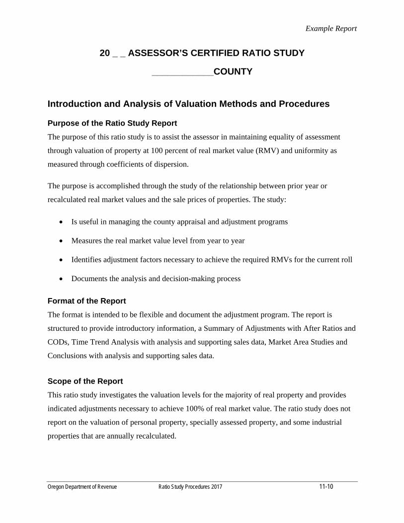
Example Report
Oregon Department of Revenue Ratio Study Procedures 2017 11-10
20 _ _ ASSESSOR’S CERTIFIED RATIO STUDY
____________COUNTY
Introduction and Analysis of Valuation Methods and Procedures
Purpose of the Ratio Study Report
The purpose of this ratio study is to assist the assessor in maintaining equality of assessment
through valuation of property at 100 percent of real market value (RMV) and uniformity as
measured through coefficients of dispersion.
The purpose is accomplished through the study of the relationship between prior year or
recalculated real market values and the sale prices of properties. The study:
Is useful in managing the county appraisal and adjustment programs
Measures the real market value level from year to year
Identifies adjustment factors necessary to achieve the required RMVs for the current roll
Documents the analysis and decision-making process
Format of the Report
The format is intended to be flexible and document the adjustment program. The report is
structured to provide introductory information, a Summary of Adjustments with After Ratios and
CODs, Time Trend Analysis with analysis and supporting sales data, Market Area Studies and
Conclusions with analysis and supporting sales data.
Scope of the Report
This ratio study investigates the valuation levels for the majority of real property and provides
indicated adjustments necessary to achieve 100% of real market value. The ratio study does not
report on the valuation of personal property, specially assessed property, and some industrial
properties that are annually recalculated.
Example Report
Oregon Department of Revenue Ratio Study Procedures 2017 11-11
Status of the Assessor’s RMV Adjustment Program
The report describes the county’s recalculation process (if utilized).
The county’s current assessment computer system is ____________________. (If in conversion,
identify new system, explain status of transition, and projected completion date.)
The assessor’s office will continue to review market information. It is possible that additional
data or further analysis will lead to different conclusions than contained in this report. Changes
to this study will be reported to the department and to the Board of Property Tax Appeals.
Number of Sales during Study Year
Total number of arm’s-length transactions during study year _________
Number of sales used in the studies _________
Number of sales confirmed and/or verified _________
Recalculation Process
The recalculation process can consider all of the numerous individual characteristics in the
valuation model. It is distinguished from appraisal by its lack of a property inspection. Market
studies (LCM, depreciation, etc.) should be similar or the same as those used in an appraisal
setup. Both recalculation and traditional trending accomplish the task of adjusting the assessment
roll to a statistical 100% of RMV each year without a physical in-field verification of property
characteristics.
The county must be able to explain the recalculation process to the taxpayer and is required to
include an explanation of the methods in the ratio study report.
ORS 306.255 Information for taxpayers concerning property taxes, appraisals and appeals. (1) The county assessor shall provide and make available to taxpayers, upon request, the following information:
(b) An explanation of the methods of appraisal generally and, if of interest to the taxpayer, the method or methods of valuation of the type of property with which the taxpayer is concerned.
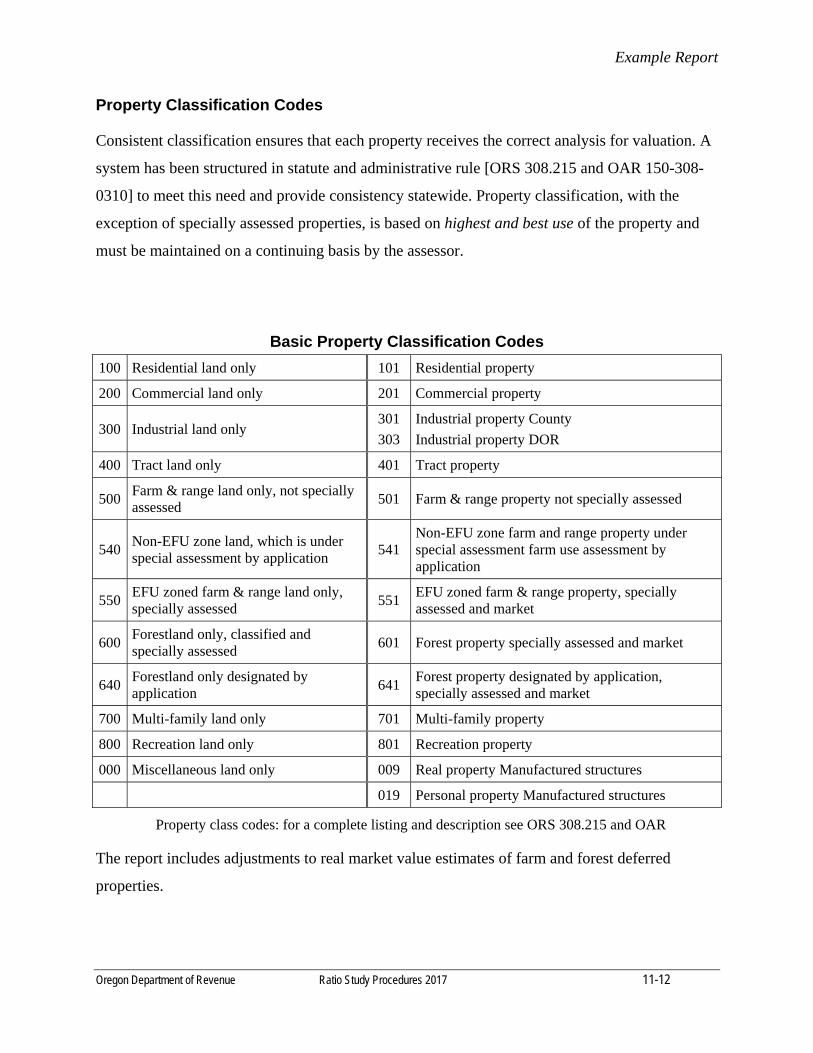
Example Report
Oregon Department of Revenue Ratio Study Procedures 2017 11-12
Property Classification Codes
Consistent classification ensures that each property receives the correct analysis for valuation. A
system has been structured in statute and administrative rule [ORS 308.215 and OAR 150-308-
0310] to meet this need and provide consistency statewide. Property classification, with the
exception of specially assessed properties, is based on highest and best use of the property and
must be maintained on a continuing basis by the assessor.
Basic Property Classification Codes
100 Residential land only 101 Residential property
200 Commercial land only 201 Commercial property
300 Industrial land only 301
303
Industrial property County
Industrial property DOR
400 Tract land only 401 Tract property
500 Farm & range land only, not specially assessed
501 Farm & range property not specially assessed
540 Non-EFU zone land, which is under special assessment by application
541 Non-EFU zone farm and range property under special assessment farm use assessment by application
550 EFU zoned farm & range land only, specially assessed
551 EFU zoned farm & range property, specially assessed and market
600 Forestland only, classified and specially assessed
601 Forest property specially assessed and market
640 Forestland only designated by application
641 Forest property designated by application, specially assessed and market
700 Multi-family land only 701 Multi-family property
800 Recreation land only 801 Recreation property
000 Miscellaneous land only 009 Real property Manufactured structures
019 Personal property Manufactured structures
Property class codes: for a complete listing and description see ORS 308.215 and OAR
The report includes adjustments to real market value estimates of farm and forest deferred
properties.
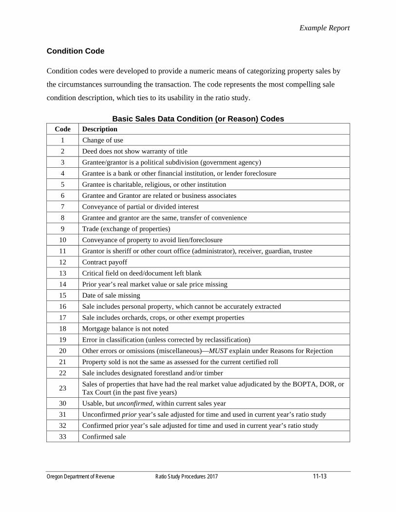
Example Report
Oregon Department of Revenue Ratio Study Procedures 2017 11-13
Condition Code
Condition codes were developed to provide a numeric means of categorizing property sales by
the circumstances surrounding the transaction. The code represents the most compelling sale
condition description, which ties to its usability in the ratio study.
Basic Sales Data Condition (or Reason) Codes Code Description
1 Change of use
2 Deed does not show warranty of title
3 Grantee/grantor is a political subdivision (government agency)
4 Grantee is a bank or other financial institution, or lender foreclosure
5 Grantee is charitable, religious, or other institution
6 Grantee and Grantor are related or business associates
7 Conveyance of partial or divided interest
8 Grantee and grantor are the same, transfer of convenience
9 Trade (exchange of properties)
10 Conveyance of property to avoid lien/foreclosure
11 Grantor is sheriff or other court office (administrator), receiver, guardian, trustee
12 Contract payoff
13 Critical field on deed/document left blank
14 Prior year’s real market value or sale price missing
15 Date of sale missing
16 Sale includes personal property, which cannot be accurately extracted
17 Sale includes orchards, crops, or other exempt properties
18 Mortgage balance is not noted
19 Error in classification (unless corrected by reclassification)
20 Other errors or omissions (miscellaneous)—MUST explain under Reasons for Rejection
21 Property sold is not the same as assessed for the current certified roll
22 Sale includes designated forestland and/or timber
23 Sales of properties that have had the real market value adjudicated by the BOPTA, DOR, or Tax Court (in the past five years)
30 Usable, but unconfirmed, within current sales year
31 Unconfirmed prior year’s sale adjusted for time and used in current year’s ratio study
32 Confirmed prior year’s sale adjusted for time and used in current year’s ratio study
33 Confirmed sale
Example Report
Oregon Department of Revenue Ratio Study Procedures 2017 11-14
Sales Listings
A collection of sales or market data that have been analyzed and determined to be adequate for
use in the ratio study. The collection of sales is usually organized in a standard format (see
below). Each study has a sales listing. For each sale in the listing, the property is identified,
classified and a ratio calculated.
A description of major headings in the standard format of sales listings:
Market Area: specific group of properties selected for study, i.e. residential
neighborhoods, convenience stores, retail shops
Account Number: numeric or alphanumeric property identifier
Property Class (PC): A three digit number designating type of property
Example: 1-0-0 Residential Vacant or 1-0-1 Residential Improved
Condition Code: a numeric means of categorizing property sales by the circumstances
surrounding the transaction
Map and Tax Lot: Locates the property in the county. Sales that include more than
one account display an asterisk (*) after the tax lot number.
Instrument Number: The recording number that identifies the sale document
Total RMV: This is usually the RMV from the current certified assessment roll. In
some cases it is the value that would have been on the roll although the property has
changed. Examples of such changes include construction of buildings and
consolidation with other tax lots.
Sale Price: Normally the consideration on the document transferring ownership.
Adjusted Sale Price (when applicable): The estimated sale price for the property if it
were to sell January 1, assessment date for the current study; or, if the sale price is
adjusted to remove personal property value, for example.
Sale Number: sales are ordered and each is identified with a number
Ratio: A comparison where the RMV on the certified roll for a Before Ratio (and the
recalculated RMV for an After Ratio) is divided by the Sale Price or Adjusted Sale
Price and the result is expressed as a percentage. This expresses the RMV level as of
the date of sale or as of January 1 assessment date. Example: Current RMV on the
Example Report
Oregon Department of Revenue Ratio Study Procedures 2017 11-15
certified roll: $95,000. Property sold in May for $100,000. The ratio is computed as
$95,000 ÷ $100,000 = 0.95 or a ratio of 95 percent (represents the level of valuation as
of May).
Note: The sale was not adjusted to January 1 of the current year.
Description of Report Sections
Summary of Adjustments
Summary pages list market area studies for each property classification. The summary
should specify the area(s) and the number of accounts affected by the study; report page
number; adjustment factors for land, improvements, and overall; after ratio; PRD; COD
standard for the area and the COD for the reporting year.
Market areas are listed
Residential: residential land, single family dwellings, condominiums, duplexes, tri-
plexes, four-plexes and manufactured structures
Rural: tract property, market residential improvements, farm, and forest buildings
Income: land and improvements for commercial, industrial, and multi-family
properties
Other: land and improvements that do not fit into any of the other categories:
recreational properties and mineral rights [if it is actively being mined as of the
assessment date ORS. 308.115 (2)] including site improvements
Sales Trimming
Very low or very high ratios are often called outliers. Outliers require additional scrutiny
to identify whether the sale is a non-market transaction or an extreme event that may tend
to skew the results of the study.
Standard statistical trimming methods (Trimmed Mean and Interquartile Range) are
recognized as a means to identify and remove certain outliers from sales listings used in
Example Report
Oregon Department of Revenue Ratio Study Procedures 2017 11-16
market analysis. Trimming is not mandatory but when appropriate, it is performed before
all other studies.
Change in Market Conditions Over Time (Time Study)
Fluctuating market conditions may create the need to apply an adjustment to sales prices
that occurred during the sales year. Although the adjustment is often called a time
adjustment, time itself is not the reason for the adjustment; it is the movement of value
over time. The adjustment is expressed as a percentage of increase or decrease to sales
prices to reflect what the property would have sold for as of the assessment date.
This section includes trend analysis and documented support for the conclusions. The
data is usually presented in graphic form by month and/or quarter followed by a narrative
conclusion. Time trends may be developed for various property classes but usually apply
to residential properties.
Market Area Studies (Analysis Pages)
Each study should include a map of the study area, market area identifier (name, code
number, etc.), description of the physical location, and the property classification(s)
studied. Describe land characteristics, dominate age, type of improvements, and the last
year physically appraised.
The analysis pages include:
Number of accounts in the study area
Number of sales used for the study
Measures of central tendency calculated for the sales
o Median: the middle of the array, influenced only by the position of the ratios in the array, not by their values
o Mean (Arithmetic Mean): the simple average of the individual ratios in the sales array
o Weighted Mean: derived by dividing the total of the current certified roll RMVs or recalculated value of the sales by the total of the sale prices in the array
Narrative description for the selection of the measure of central tendency considered
Example Report
Oregon Department of Revenue Ratio Study Procedures 2017 11-17
most representative of the market study area. Note: No single sale should have a
large influence on the selected central tendency.
o Avoid a MEAN distorted by extreme ratios
o Avoid a WEIGHTED MEAN influenced by high valued properties at either end of the array
o Avoid a MEDIAN when gaps exist in the middle of the frequency distribution
Calculated overall adjustment factor. (When a time adjustment is applied to the
selected central tendency, the adjustment information will be included on the
analysis page.)
For improved properties, the overall adjustment factor may be weighted and applied
to the individual RMV components (land, OSD, farm buildings, major
improvements)
o A correct overall adjustment factor will result in half the properties being over market and half being under market but does not test uniformity in valuation (which is measured by CODs)
o A single adjustment factor applied to all components cannot reduce the distribution of ratios within a property class or improve the COD
o Weighting by percentage of the individual RMV components may be applied when sufficient data is available and may improve COD
Histogram showing frequency of sales ratios before and after adjustments: a visual
aid used to display distribution of ratios and gives an indication of the degree of
uniformity
Coefficient of Dispersion (COD): average deviation from the median converted to a
percentage. It measures uniformity of real market value levels.
Price Related Differential (PRD): used to evaluate whether RMVs are reasonably
uniform between high and low valued properties
Current and 3-5 year performance history for COD and PRD
Example Report
Oregon Department of Revenue Ratio Study Procedures 2017 11-18
COUNTY MAP
and
MAPS OF MARKET AREAS AS APPROPRIATE
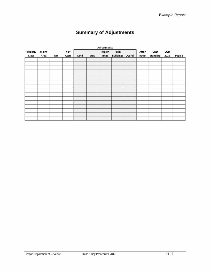
Example Report
Oregon Department of Revenue Ratio Study Procedures 2017 11-19
Summary of Adjustments
Property
Class
Maint
Area NH
# of
Accts Land OSD
Major
Imps
Farm
Buildings Overall
After
Ratio
COD
Standard
COD
2016 Page #
Adjustments
Example Report
Oregon Department of Revenue Ratio Study Procedures 2017 11-20
Sales Trimming Method and List of Sales Trimmed
Method used for trimming sales:
List of arm’s-length transactions trimmed:
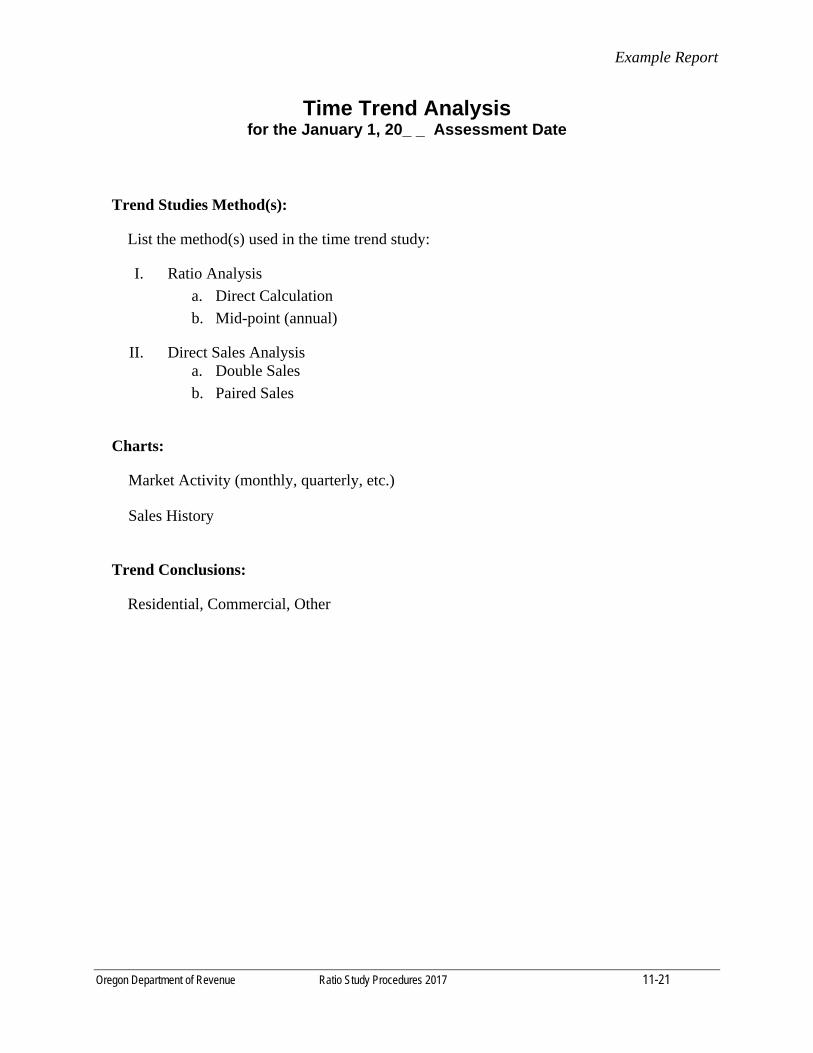
Example Report
Oregon Department of Revenue Ratio Study Procedures 2017 11-21
Time Trend Analysis for the January 1, 20_ _ Assessment Date
Trend Studies Method(s):
List the method(s) used in the time trend study:
I. Ratio Analysis
a. Direct Calculation
b. Mid-point (annual)
II. Direct Sales Analysis a. Double Sales
b. Paired Sales
Charts:
Market Activity (monthly, quarterly, etc.)
Sales History
Trend Conclusions:
Residential, Commercial, Other
Example Report
Oregon Department of Revenue Ratio Study Procedures 2017 11-22
Market Area Studies
(Analysis Pages)
Example Report
Oregon Department of Revenue Ratio Study Procedures 2017 11-23
For each market study area include the following:
Map of market study area
Description of the market study area
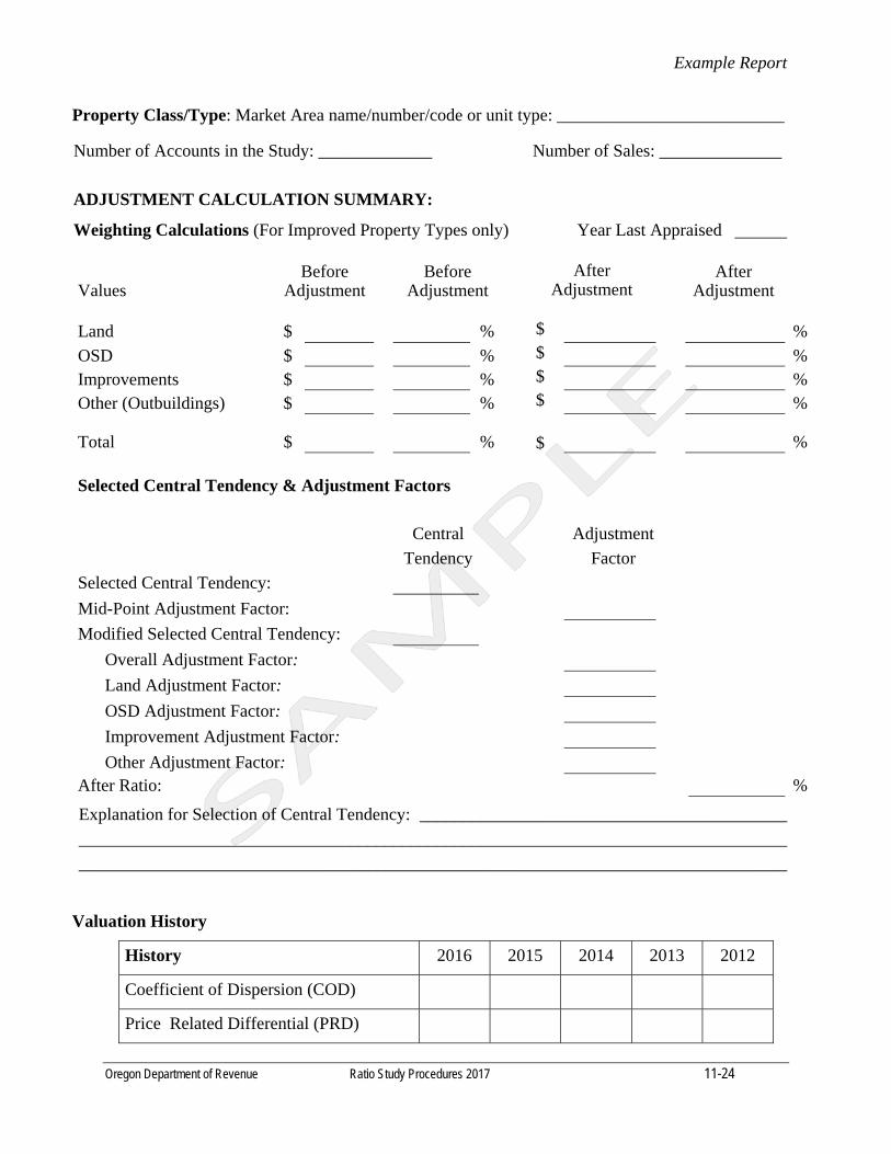
Example Report
Oregon Department of Revenue Ratio Study Procedures 2017 11-24
Property Class/Type: Market Area name/number/code or unit type: __________________________
Number of Accounts in the Study: _____________ Number of Sales: ______________
ADJUSTMENT CALCULATION SUMMARY:
Weighting Calculations (For Improved Property Types only) Year Last Appraised
Values Before
AdjustmentBefore
AdjustmentAfter
Adjustment
After
Adjustment
Land $ % $ %
OSD $ % $ %Improvements $ % $ %Other (Outbuildings) $ % $ % Total $ % $ %
Selected Central Tendency & Adjustment Factors
Central
Tendency
Adjustment
Factor
Selected Central Tendency:
Mid-Point Adjustment Factor:
Modified Selected Central Tendency:
Overall Adjustment Factor:
Land Adjustment Factor:
OSD Adjustment Factor:
Improvement Adjustment Factor:
Other Adjustment Factor: After Ratio: %
Explanation for Selection of Central Tendency: __________________________________________
_________________________________________________________________________________
_________________________________________________________________________________
Valuation History
History 2016 2015 2014 2013 2012
Coefficient of Dispersion (COD)
Price Related Differential (PRD)
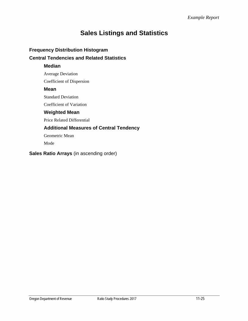
Example Report
Oregon Department of Revenue Ratio Study Procedures 2017 11-25
Sales Listings and Statistics
Frequency Distribution Histogram
Central Tendencies and Related Statistics
Median
Average Deviation
Coefficient of Dispersion
Mean
Standard Deviation
Coefficient of Variation
Weighted Mean
Price Related Differential
Additional Measures of Central Tendency
Geometric Mean
Mode
Sales Ratio Arrays (in ascending order)
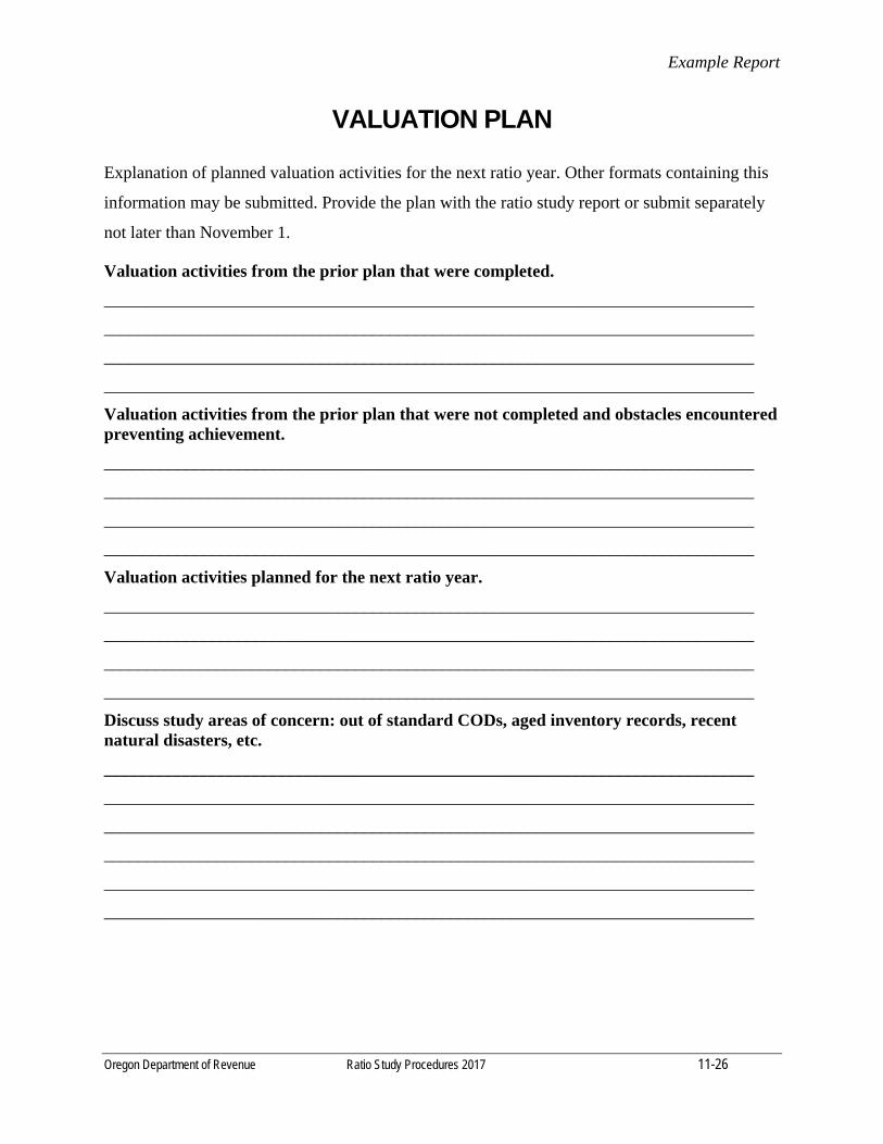
Example Report
Oregon Department of Revenue Ratio Study Procedures 2017 11-26
VALUATION PLAN
Explanation of planned valuation activities for the next ratio year. Other formats containing this
information may be submitted. Provide the plan with the ratio study report or submit separately
not later than November 1.
Valuation activities from the prior plan that were completed.
___________________________________________________________________________
___________________________________________________________________________
___________________________________________________________________________
___________________________________________________________________________
Valuation activities from the prior plan that were not completed and obstacles encountered preventing achievement.
___________________________________________________________________________
___________________________________________________________________________
___________________________________________________________________________
___________________________________________________________________________
Valuation activities planned for the next ratio year.
___________________________________________________________________________
___________________________________________________________________________
___________________________________________________________________________
___________________________________________________________________________
Discuss study areas of concern: out of standard CODs, aged inventory records, recent natural disasters, etc.
___________________________________________________________________________
___________________________________________________________________________
___________________________________________________________________________
___________________________________________________________________________
___________________________________________________________________________
___________________________________________________________________________
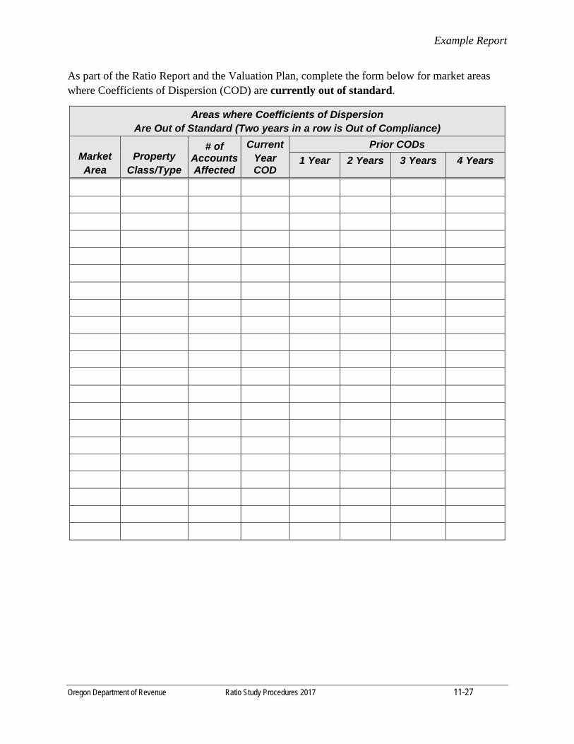
Example Report
Oregon Department of Revenue Ratio Study Procedures 2017 11-27
As part of the Ratio Report and the Valuation Plan, complete the form below for market areas where Coefficients of Dispersion (COD) are currently out of standard.
Areas where Coefficients of Dispersion Are Out of Standard (Two years in a row is Out of Compliance)
Market Area
Property Class/Type
# of Accounts Affected
CurrentYear COD
Prior CODs
1 Year 2 Years 3 Years 4 Years


Oregon Department of Revenue Ratio Study Procedures 2017 12-1
SECTION 12
STATUTES AND RULES
RELATING TO COUNTY RATIO STUDIES
ORS 192.430 Functions of custodian of public records; rules. (1) The custodian of any public records, including public records maintained in machine readable or electronic form, unless otherwise expressly provided by statute, shall furnish proper and reasonable opportunities for inspection and examination of the records in the office of the custodian and reasonable facilities for making memoranda or abstracts therefrom, during the usual business hours, to all persons having occasion to make examination of them. If the public record is maintained in machine readable or electronic form, the custodian shall furnish proper and reasonable opportunity to assure access. (2) The custodian of the records may adopt reasonable rules necessary for the protection of the records and to prevent interference with the regular discharge of duties of the custodian. [1973 c.794 §4; 1989 c.546 §1]
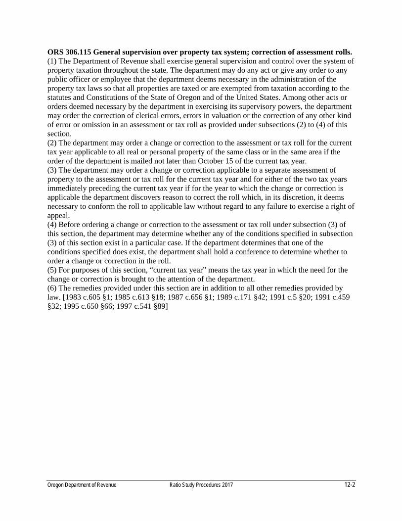
Oregon Department of Revenue Ratio Study Procedures 2017 12-2
ORS 306.115 General supervision over property tax system; correction of assessment rolls. (1) The Department of Revenue shall exercise general supervision and control over the system of property taxation throughout the state. The department may do any act or give any order to any public officer or employee that the department deems necessary in the administration of the property tax laws so that all properties are taxed or are exempted from taxation according to the statutes and Constitutions of the State of Oregon and of the United States. Among other acts or orders deemed necessary by the department in exercising its supervisory powers, the department may order the correction of clerical errors, errors in valuation or the correction of any other kind of error or omission in an assessment or tax roll as provided under subsections (2) to (4) of this section. (2) The department may order a change or correction to the assessment or tax roll for the current tax year applicable to all real or personal property of the same class or in the same area if the order of the department is mailed not later than October 15 of the current tax year. (3) The department may order a change or correction applicable to a separate assessment of property to the assessment or tax roll for the current tax year and for either of the two tax years immediately preceding the current tax year if for the year to which the change or correction is applicable the department discovers reason to correct the roll which, in its discretion, it deems necessary to conform the roll to applicable law without regard to any failure to exercise a right of appeal. (4) Before ordering a change or correction to the assessment or tax roll under subsection (3) of this section, the department may determine whether any of the conditions specified in subsection (3) of this section exist in a particular case. If the department determines that one of the conditions specified does exist, the department shall hold a conference to determine whether to order a change or correction in the roll. (5) For purposes of this section, “current tax year” means the tax year in which the need for the change or correction is brought to the attention of the department. (6) The remedies provided under this section are in addition to all other remedies provided by law. [1983 c.605 §1; 1985 c.613 §18; 1987 c.656 §1; 1989 c.171 §42; 1991 c.5 §20; 1991 c.459 §32; 1995 c.650 §66; 1997 c.541 §89]

Oregon Department of Revenue Ratio Study Procedures 2017 12-3
ORS 306.120 Uniform methods of assessment; continuing study of equalization. The Department of Revenue shall: (1) Issue regulations, bulletins, manuals, instructions and directions to county assessors, county boards of property tax appeals and tax collectors as to the methods best calculated to secure uniformity according to law, in the system of assessment and collection of taxes. (2) Carry on a continuing study with the object of equalizing for the purposes of assessment and taxation property values within the counties and between the counties. [Amended by 1997 c.541 §94]
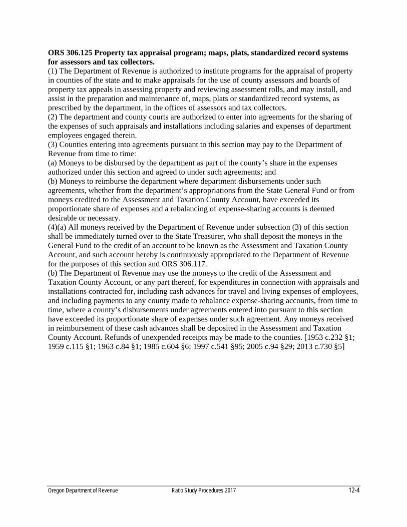
Oregon Department of Revenue Ratio Study Procedures 2017 12-4
ORS 306.125 Property tax appraisal program; maps, plats, standardized record systems for assessors and tax collectors. (1) The Department of Revenue is authorized to institute programs for the appraisal of property in counties of the state and to make appraisals for the use of county assessors and boards of property tax appeals in assessing property and reviewing assessment rolls, and may install, and assist in the preparation and maintenance of, maps, plats or standardized record systems, as prescribed by the department, in the offices of assessors and tax collectors. (2) The department and county courts are authorized to enter into agreements for the sharing of the expenses of such appraisals and installations including salaries and expenses of department employees engaged therein. (3) Counties entering into agreements pursuant to this section may pay to the Department of Revenue from time to time: (a) Moneys to be disbursed by the department as part of the county’s share in the expenses authorized under this section and agreed to under such agreements; and (b) Moneys to reimburse the department where department disbursements under such agreements, whether from the department’s appropriations from the State General Fund or from moneys credited to the Assessment and Taxation County Account, have exceeded its proportionate share of expenses and a rebalancing of expense-sharing accounts is deemed desirable or necessary. (4)(a) All moneys received by the Department of Revenue under subsection (3) of this section shall be immediately turned over to the State Treasurer, who shall deposit the moneys in the General Fund to the credit of an account to be known as the Assessment and Taxation County Account, and such account hereby is continuously appropriated to the Department of Revenue for the purposes of this section and ORS 306.117. (b) The Department of Revenue may use the moneys to the credit of the Assessment and Taxation County Account, or any part thereof, for expenditures in connection with appraisals and installations contracted for, including cash advances for travel and living expenses of employees, and including payments to any county made to rebalance expense-sharing accounts, from time to time, where a county’s disbursements under agreements entered into pursuant to this section have exceeded its proportionate share of expenses under such agreement. Any moneys received in reimbursement of these cash advances shall be deposited in the Assessment and Taxation County Account. Refunds of unexpended receipts may be made to the counties. [1953 c.232 §1; 1959 c.115 §1; 1963 c.84 §1; 1985 c.604 §6; 1997 c.541 §95; 2005 c.94 §29; 2013 c.730 §5]
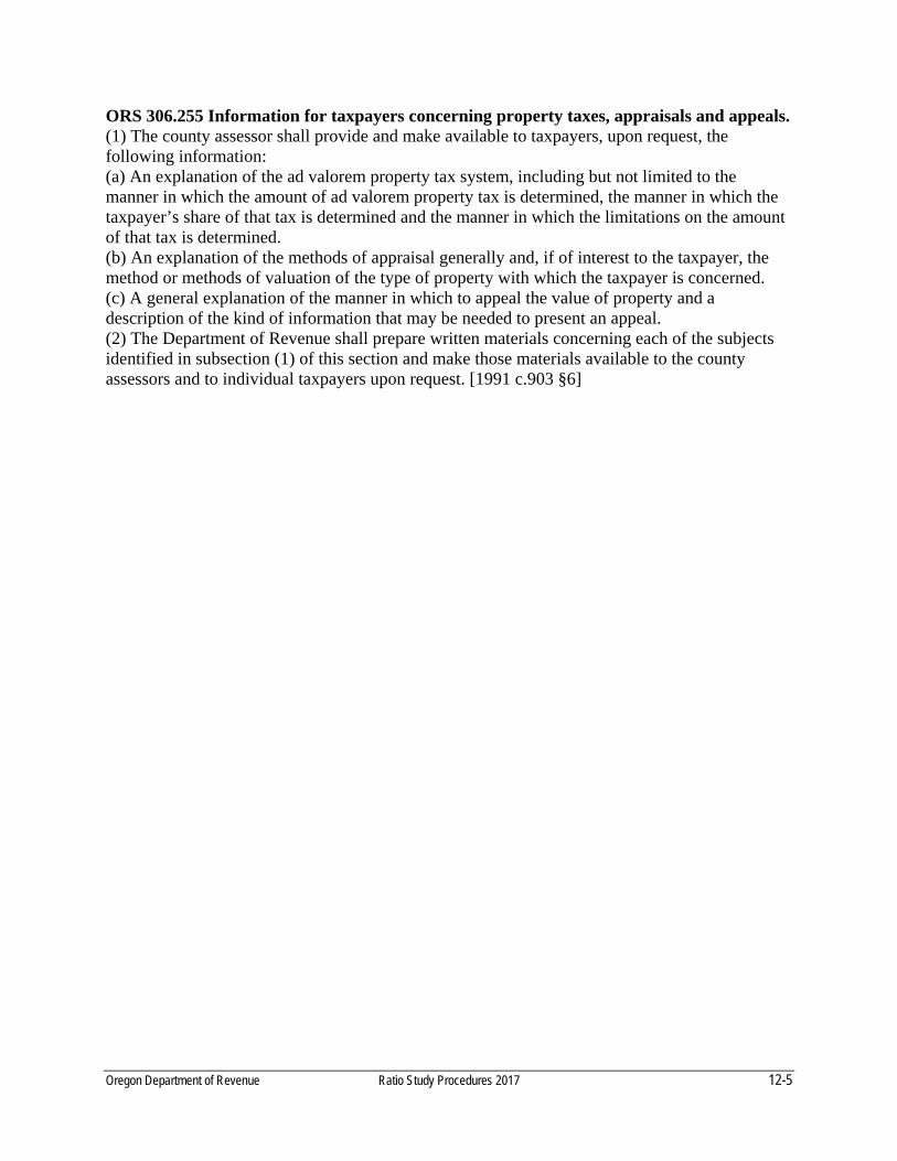
Oregon Department of Revenue Ratio Study Procedures 2017 12-5
ORS 306.255 Information for taxpayers concerning property taxes, appraisals and appeals. (1) The county assessor shall provide and make available to taxpayers, upon request, the following information: (a) An explanation of the ad valorem property tax system, including but not limited to the manner in which the amount of ad valorem property tax is determined, the manner in which the taxpayer’s share of that tax is determined and the manner in which the limitations on the amount of that tax is determined. (b) An explanation of the methods of appraisal generally and, if of interest to the taxpayer, the method or methods of valuation of the type of property with which the taxpayer is concerned. (c) A general explanation of the manner in which to appeal the value of property and a description of the kind of information that may be needed to present an appeal. (2) The Department of Revenue shall prepare written materials concerning each of the subjects identified in subsection (1) of this section and make those materials available to the county assessors and to individual taxpayers upon request. [1991 c.903 §6]
Oregon Department of Revenue Ratio Study Procedures 2017 12-6
308.062 Action by department when appraisals not being conducted as provided by law; reimbursement of department costs. (1) If the Department of Revenue determines that appraisals in any county are not being made as provided by law, to meet the requirements of real market value and under a program that ensures compliance with ORS 308.234, or if the department determines that the county is not in compliance with a conference agreement or a plan developed at a conference as provided under ORS 294.181, it shall make a written report to the county court or board of county commissioners of the county, describing the provisions of law which are not being followed and recommending specific measures to be taken by the county court or board and the assessor to cure the deficiencies noted. (2) If the department thereafter discovers that any measure or measures are not being taken as recommended under subsection (1) of this section, and that as a result, in the department’s opinion, appraisals in the county are not being made as provided by law, including meeting the requirements of ORS 308.232 or 308.234, the department shall give 30 days’ written notice to the assessor and to the county court or board of county commissioners of its intention to use the most practicable means to cure the deficiencies, including but not limited to the use of its own employees and equipment or the use of fee appraisers. If within the 30-day period the assessor and the county court or board of county commissioners fail to take action to correct the deficiencies through the providing of funds and personnel, or by the submission of a plan acceptable to the department, the department shall proceed to cure the deficiencies. The county court or board of county commissioners shall bear the full expense of the necessary actions taken by the Department of Revenue for the benefit of the county, aided by the provisions of subsection (3) of this section. (3) In the event that the department must perform services within or for a county pursuant to subsection (2) of this section, the costs shall be advanced from its Assessment and Taxation County Account, described in ORS 306.125, and, except as otherwise provided by law, that account shall be reimbursed for the sum of such costs from the county’s share of the state shared funds, unless other provision is made by action of the county court or board. Reimbursement of the Assessment and Taxation County Account shall be made from time to time upon the order of the Secretary of State to the State Treasurer, based upon the Department of Revenue’s certified, itemized statement of such costs to the Secretary of State. Reimbursement shall be from an equal proportion of all state share funds required or permitted to be distributed to the county that are not otherwise dedicated as provided by law. If the county is a county for which expenditures for assessment and taxation have been certified under ORS 294.175, the total reimbursement to the department shall not exceed the amount of the expenditures so certified. If the county is a county for which expenditures for assessment and taxation have not been certified under ORS 294.175, the total reimbursement to the department shall not exceed the total amount of expenditures as determined for purposes of issuing the notice required under ORS 294.175 (4). Copies of the department’s certified itemized statement of costs shall be sent to the county court or board and to the county assessor. [1989 c.796 §18; 1991 c.459 §175; 1997 c.782 §8; 2003 c.169 §10]
Oregon Department of Revenue Ratio Study Procedures 2017 12-7
ORS 308.205 Real market value defined; rules. (1) Real market value of all property, real and personal, means the amount in cash that could reasonably be expected to be paid by an informed buyer to an informed seller, each acting without compulsion in an arm’s-length transaction occurring as of the assessment date for the tax year. (2) Real market value in all cases shall be determined by methods and procedures in accordance with rules adopted by the Department of Revenue and in accordance with the following: (a) The amount a typical seller would accept or the amount a typical buyer would offer that could reasonably be expected by a seller of property. (b) An amount in cash shall be considered the equivalent of a financing method that is typical for a property. (c) If the property has no immediate market value, its real market value is the amount of money that would justly compensate the owner for loss of the property. (d) If the property is subject to governmental restriction as to use on the assessment date under applicable law or regulation, real market value shall not be based upon sales that reflect for the property a value that the property would have if the use of the property were not subject to the restriction unless adjustments in value are made reflecting the effect of the restrictions. [Amended by 1953 c.701 §2; 1955 c.691 §§1, 2; 1977 c.423 §2; 1981 c.804 §34; 1989 c.796 §30; 1991 c.459 §88; 1993 c.19 §6; 1997 c.541 §152] OAR 150-308-0240 Real Property Valuation for Tax Purposes (1) For the purposes of this rule, the following words and phrases have the following meaning: (e) "Highest and best use" means the reasonably probable and legal use of vacant land or an improved property that is physically possible, appropriately supported, and financially feasible, and that results in the highest value. See The Appraisal of Real Estate, 12th edition (2001). (e) "Highest and best use" means the reasonably probable use of vacant land or an improved property that is legally permissible, physically possible, financially feasible, and maximally productive, which results in the highest real market value.
Oregon Department of Revenue Ratio Study Procedures 2017 12-8
ORS 308.215 Contents of assessment roll; rules. (1) The assessor shall prepare the assessment roll in the following form: (a) Real property shall be listed in sequence by account number or by code area and account numbers. For each parcel of real property, the assessor shall set down in the assessment roll according to the best information the assessor can obtain: (A) The name of the owner or owners and, if the assessor or tax collector is instructed in writing by the owner or owners to send statements and notices relating to taxation to an agent or representative, the name of such agent or representative. (B) A description as required by ORS 308.240 with its code area and account numbers. (C) The property class, in accordance with the classes established by rule by the Department of Revenue. (D) The number of acres and parts of an acre, as nearly as can be ascertained, unless it is divided into blocks and lots. (E) The real market value of the land, excluding all buildings, structures, improvements and timber thereon. (F) The real market value of all buildings, structures and improvements thereon. (G) The real market value of each unit together with its percentage of undivided interest in the common elements of property subject to ORS 100.005 to 100.910 stating separately the real market value of the land, buildings, structures and improvements of each unit. (H) For each parcel of real property granted an exemption under ORS 307.250 to 307.283, the real market value so exempt. (I) The total assessed value, maximum assessed value and real market value of each parcel of real property assessed. (b) For personal property, the assessor shall set down separately in the assessment roll, according to the best information the assessor can obtain: (A) The names, including assumed business names, if any, of all persons, whether individuals, partnerships or corporations, or other owner, owning or having possession or control of taxable personal property on January 1, at 1:00 a.m. of the assessment year. If it is a partnership, the names of two general partners and the total number thereof. (B) The real market value of the personal property assessed, with a separate value for each category of personal property, if any. The Department of Revenue, by rule, may establish such categories as appear useful or necessary for good tax administration. (C) The number of the code area assigned by the assessor covering the situs of the property on January 1. (D) The total assessed, maximum assessed and real market value for the property. (c) Real property and machinery and equipment listed on the assessment roll shall each bear a distinctive designation so that machinery and equipment can be identified with the real property upon which the machinery and equipment is located. (d)(A) The listing of manufactured structures on the assessment roll, whether as real or personal property, shall be done in a distinctive manner so that manufactured structures may be readily distinguished from other property. (B) In lieu of listing manufactured structures on the assessment roll as real or personal property, the assessor may list manufactured structures in a separate section of the assessment roll. In any county where such separate listing of manufactured structures is made the manufactured structures assessed as real property under ORS 308.875 shall bear a distinctive designation so that it can be identified with the real property upon which it is located. In like manner the real
Oregon Department of Revenue Ratio Study Procedures 2017 12-9
property upon which the manufactured structure is situated shall bear a distinctive designation so that it can be identified with the manufactured structure. Where a homestead exemption is granted to a manufactured structure assessed as real property under ORS 308.875, which manufactured structure is listed on a portion of the assessment roll separate from the real property, the exempt amount shall apply first to the value of the manufactured structure, and any remainder shall apply to the parcel of land upon which it is situated. (2) For purposes of the classification of real property required under subsection (1)(a)(C) of this section, property listed in paragraph (a), (b) or (c) of this subsection must be classified, together with any other property listed in the respective paragraph, separately from all other property: (a) Machinery and equipment. (b) Property appraised under ORS 306.126, other than machinery and equipment. (c) Industrial property, other than property appraised under ORS 306.126, and commercial property. (3) The Department of Revenue may by rule require that the assessment roll include information in addition to that required by subsection (1) of this section. [Amended by 1957 c.324 §2; 1963 c.270 §1; 1963 c.541 §43; 1965 c.344 §1; 1967 c.568 §1; 1971 c.529 §13; 1971 c.568 §1; 1971 c.747 §16; 1977 c.718 §6; 1979 c.692 §3; 1981 c.804 §36; 1983 s.s. c.5 §3; 1985 c.350 §1; 1985 c.613 §7; 1991 c.459 §91; 1997 c.541 §155; 1999 c.579 §4; 2012 c.30 §1] 150-308-0310 Real Market Value and Property Classification as Part of Assessment Roll (1) In addition to the assessed value of property, the assessment roll must show: (a) The real market value (RMV) of the land, excluding all buildings, structures, and improvements thereon; (b) The RMV of all buildings, structures, and improvements; and (c) The total RMV for each parcel of real property not required to be assessed as a unit. (d) For properties subject to ORS Chapter 100, for example, condominiums and time shares that are required to be assessed as a unit, the assessment roll must show the RMV as well as the assessed value of each unit. (2) The assessment roll must include the property classification code number for each parcel of real property in the county, except for those properties assessed by the department under ORS 308.505 to 308.665. The assessor must classify and assign a property classification code number to each parcel as provided in section (8) of this rule. (3) The assessor must maintain the proper classification on each parcel of property. (4) A county must separately identify and adjust land and improvement values for each property class for each market area to bring real property to RMV. These adjustments to value must be developed from market studies or by any other method approved by the department as provided under ORS 309.200. (5) The class code numbers that this rule establishes must be used for computing the real property class ratios required by ORS 309.200. (6) An assessor must obtain written approval from the Department of Revenue before deviating from the basic property classes defined in section (8) of this rule. (7)(a) All classification must be based upon highest and best use of the property. The term “highest and best use” is defined in OARs 150-308-0240 and 150-308-0260. The class associated with the property may or may not be its current use.

Oregon Department of Revenue Ratio Study Procedures 2017 12-10
(b) Unique properties can be classified under the “miscellaneous” category in section (8). The “miscellaneous” category can also be used for property requiring a separate trend. (c) The property classification system must not be used to categorize market data that is more accurately described by other characteristics, such as the quality class of the improvements, market areas, or neighborhoods. (d) The property class for mixed-use or transitional properties will be assigned based upon the use that contributes the most to the real market value on the current assessment date. (A) A mixed-use property is one in which different parts of the property are used differently, such as a commercial use on one part, and a residential use on another part. (B) A transitional use property is one in which the real market value on the current assessment date, at its current highest and best use, is being influenced in the market by an anticipated change in future use, such as residential property that is likely to sell for a commercial use in the future, but is not in commercial use on the assessment date. (8) DEFINITIONS FOR PROPERTY CLASSIFICATION SYSTEM. [Classification not included. See ED. NOTE.] (9) Starting with the 2006–07 tax year, each assessor must prepare an annual plan that outlines how the county will comply with the provisions of this rule no later than the January 1, 2009 assessment date. The plan must be submitted as part of the sales ratio study and accompanying appraisal plan submitted under ORS 309.200 and 309.203. The plan must address how the county complies with, or intends to comply with the provisions of this rule for the initial tax year and all subsequent tax years up to the 2009–2010 tax year. [ED. NOTE: Classification referenced is available from the agency.] Stat. Auth.: ORS 305.100, 308.215 Stats. Implemented: ORS 308.215 Hist.: 3-70; 9-71; 11-73; 1-1-77; TC 10-1978, f. 12-5-78, cert. ef. 12-31-78; TC 17-1979, f. 12-20-79, cert. ef. 12-31-79; RD 9-1984, f. 12-5-84, cert. ef. 12-31-84; RD 16-1987, f. 12-10-87, cert. ef. 12-31-87; RD 9-1989, f. 12-18-89, cert. ef. 12-31-89; RD 8-1991, f. 12-30-91, cert. ef. 12-31-91; RD 6-1993, f. 12-30-93, cert. ef. 12-31-93, Renumbered from 150-308.215(1); RD 6-1994, f. 12-15-94, cert. ef. 12-30-94; RD 1-1995, f. 12-29-95, cert. ef. 12-31-95; RD 9-1997, f. & cert. ef. 12-31-97; REV 11-2000, f. 12-29-00, cert. ef. 12-31-00; REV 2-2002, f. 6-26-02, cert. ef. 6-30-02; REV 2-2005, f. 6-27-05, cert. ef 6-30-05; REV 4-2006, f. & cert .ef. 7-31-06; Renumbered from 150-308.215(1)-(A), REV 57-2016, f. 8-13-16, cert. ef. 9-1-16
Oregon Department of Revenue Ratio Study Procedures 2017 12-11
ORS 308.232 Property to be valued at 100 percent real market value and assessed at assessed value. All real or personal property within each county not exempt from ad valorem property taxation or subject to special assessment shall be valued at 100 percent of its real market value. Unless the property is subject to maximum assessed value adjustment under ORS 308.149 to 308.166, the property shall be assessed at the property’s assessed value determined under ORS 308.146. [1953 c.701 §2; 1959 c.519 §1; 1961 c.243 §1; 1967 c.293 §6; 1979 c.241 §33; 1981 c.804 §39; 1985 c.613 §8; 1991 c.459 §97; 1997 c.541 §159] ORS 308.234 Record of last appraisal; Department of Revenue to approve methods of appraisal. The county assessors shall preserve in their respective offices records to show when each parcel of real property was last appraised. Each parcel of real property shall be appraised using a method of appraisal approved by the Department of Revenue by rule. [1955 c.575 §1; 1967 c.105 §1; 1967 c.293 §8; 1997 c.541 §161] 150-308-0380 Appraisal of Real Property The following constitutes standards for the valuation of real property except for property assessed under ORS 308.505 to 308.665 and ORS 308.805 to 308.820. (1) Industrial property. In the case of industrial properties, appraisals must conform with the following conditions: (a) Basic data and supplemental data for an appraisal must be the same as required in ORS 308.290 and 308.411. Valid data in any previous appraisal such as property descriptions, inventory listing, maps, etc., may be used in the appraisal. (b) An appraisal as provided by the industrial property return process is not an appraisal contemplated under ORS 308.234. (c) A valuation review as provided in OAR 150-308-0300 is an appraisal as contemplated under ORS 308.234, if the valuation review meets the requirements of 308.411. (d) Nothing in this rule is intended to invalidate any assessment that appears on the assessment roll. (2) All other real property. Real property must be valued at its real market value (RMV) using methods approved by the department and the results must meet the performance standards required by this rule. (a) The following definitions apply for the purposes of this rule: (A) "Coefficient of dispersion" (COD) is the average absolute deviation of a group of numbers from the median expressed as a percentage of the median. In ratio studies, it refers to the average absolute deviation from the median ratio, expressed as a percent of the median ratio. (B) "Homogeneous" describes a market area where the properties have a high degree of similarity in one or more of the following: type, use, quality, or condition. (C) "Market area" is defined as a group of properties that share important characteristics affecting their value. It may be defined along physical/geographical or abstract boundaries or, as in the case of commercial property, according to use. Properties included in a market area do not have to be contiguous. (D) "Nonhomogeneous" means market areas that do not meet the definition of "homogeneous."
Oregon Department of Revenue Ratio Study Procedures 2017 12-12
(b) ORS 308.232 requires that all real property be valued at 100 percent of its RMV. Achieving and maintaining RMV is measured by the ratio study. Ratios must be computed for each market area, where possible. In market areas where the amount of sales data is insufficient for statistical analysis, one or more of the following actions should be taken to provide adequate data: (A) A two-year sales sample may be used; (B) Comparable market areas may be combined; or (C) Appraisal ratio data may be included. (c) Criteria for results-based valuation standards: (A) RMV at 100 percent. (B) COD standards for measuring equity of RMV: [Formula not included. See ED. NOTE.] (C) Exceptions to COD standards. When a market area does not meet the standards because of a market anomaly, the correction may be delayed until the following year, waived, or have alternate standards applied, as approved by the Department of Revenue. (d) The department will determine compliance with standards of this rule by annual reviews of the results determined by the county. (A) If compliance deficiencies are found, the department must make written notification to the assessor of the deficiencies and identify appropriate corrective action. Within 30 days of notification of the deficiencies, the assessor must respond in writing to the department as to the action to be taken to correct the identified deficiencies. (B) In the event an assessor's program has been found to be deficient and the assessor does not take action to correct the deficiencies as outlined in the department's written notification, the department will take action as required by ORS 308.062. [ED. NOTE: Formulas referenced are not included in rule text. Click here for PDF copy of formula(s).] Stat. Auth.: ORS 305.100 Stats. Implemented: ORS 308.234 Hist.: 8-65; 1-66; 3-70; 9-70; 9-71; 8-72; TC 10-1978, f. 12-5-78, cert. ef. 12-31-78; REV 4-1998, f. & cert. ef. 6-30-98; REV 9-1998, f. 12-11-98, cert. ef. 12-31-98; REV 12-1998, f. 12-29-98, cert. ef. 12-31-98; REV 6-2001, f. & cert. ef. 12-31-01; REV 11-2010, f. 7-23-10, cert. ef. 7-31-10; Renumbered from 150-308.234, REV 57-2016, f. 8-13-16, cert. ef. 9-1-16
Oregon Department of Revenue Ratio Study Procedures 2017 12-13
ORS 309.200 Assessor to collect sales data and prepare ratio study; filing study with board and department. (1) Between January 1 and December 31 of each year the county assessor shall collect sales data for a ratio study. (2) The assessor shall prepare and complete a certified ratio study in the time and manner provided by the rules adopted by the Department of Revenue. A copy of the sales data collected and used as the basis for conclusions relating to real market value shall be included with the ratio study. The assessor shall file a certified copy of the sales data and ratio study with the department, as prescribed by department rule. (3) Not later than October 15 of each year the assessor shall file with the clerk of the board of property tax appeals a copy of the ratio study. [1975 c.753 §2; 1981 c.804 §23; 1985 c.613 §24; 1989 c.330 §18; 1991 c.459 §202; 1993 c.270 §43; 1997 c.541 §239; 1999 c.655 §7] 150-309-0230 Assessor’s Ratio Study for Tax Purposes: Definitions (1) Appraisal area is an area in a county generally composed of one or more school districts, a city or other political subdivision, or any other logical division established by the county assessor for conducting an orderly reappraisal of taxable property as required by ORS 308.234. (2) A market area is a group of properties that generally shares important characteristics that influence value. Each market area should contain a sufficient number of accounts to ensure an adequate sale sample for analysis. (3) Appraisal ratio is the percentage relationship between the real market value for the prior year and an estimate of the current year’s real market value made by a qualified appraiser for a particular property. (4) Appraisal ratio study is a statistical compilation of appraisal ratios for a representative group of properties in the county randomly selected on a property class basis to produce an indication of the ratio of the prior year’s real market value to the current year’s real market value for all taxable properties in a particular class of property within the county, in a particular class of property within an appraisal area, or in a particular class of property within a market area. (5) Assessor’s ratio study is required to be filed with the clerk of the board of property tax appeals. (6) Class is a classification of property described in OAR 150-308-0310. (7) Current assessment roll is the roll being prepared for the tax year beginning July 1, of the current calendar year. (8) Current real market value is the property’s real market value, or for specially assessed properties the statutory value, as of the January 1, assessment date for which the roll is being prepared. (9) New construction is a new structure or structures added to the current assessment roll or value added by completion of construction, remodeling, renovation or other physical improvement of existing property. (10) Properties added to the roll are any properties on the current assessment roll which were not assessed on the prior year’s roll. They include value added by changed status of specially assessed properties and value added through partitioning or subdividing properties. (11) Qualified appraiser is an appraiser registered pursuant to ORS 308.010 or who is licensed or certified under 674.310.
Oregon Department of Revenue Ratio Study Procedures 2017 12-14
(12) Ratio study is a study which estimates: (a) The percentage relationship between the total prior year’s real market value of each class of taxable property on the prior assessment roll and the total current real market value of the same properties in each class on the current assessment roll; and (b) The percentage relationship between the total prior year’s real market value of each class of taxable property on the prior assessment roll and the total current real market value of the same properties in each class on the current assessment roll within each appraisal area, or market area. (13) Sales ratio is the percentage relationship between the real market value for the prior assessment year and the selling price for a particular property. (14) Sales ratio study is a statistical compilation of sales ratios designed to produce an indication of the real market value ratio of each property class, and the real market value ratio of each property class within each appraisal area, or market area. (15) Taxable property includes all locally assessed property, real and personal, not exempt from taxation (whether appraised by the assessor or the Department of Revenue). It does not include properties assessed by the Department of Revenue pursuant to ORS 308.505 to 308.660. (16) Real market value ratio is the percentage relationship between the prior year’s real market value of a class of taxable property on the prior assessment roll and the current real market value of the same property on the current assessment roll. Stat. Auth.: ORS 305.100 Stats. Implemented: ORS 309.200 Hist.: 12-19-75; TC 17-1979, f. 12-20-79, cert. ef. 12-31-79; RD 9-1984, f. 12-5-84, cert. ef. 12-31-84; RD 9-1989, f. 12-18-89, cert. ef. 12-31-89; RD 2-1996, f. 12-23-96, cert. ef. 12-31-96; RD 9-1997, f. & cert. ef. 12-31-97; Renumbered from 150-309.200-(A), REV 26-2016, f. 8-12-16, cert. ef. 9-1-16 150-309-0240 Contents of the Assessor’s Certified Ratio Study The Assessor’s Certified Ratio Study shall be prepared in accordance with OAR 150-309-0250, completed according to instructions provided by the Department of Revenue, and consist of the following items: (1) Table of Contents. (2) Certification of assessor’s ratio study and adjustment program. (3) Analysis of valuation methods and procedures. (4) Introduction (purpose of report, format of the report, etc.). (5) Reconciliation of real market value forecast analysis. (6) Time trend analysis. (7) County map showing appraisal areas. (8) Listing of property class codes and descriptions. If the county has not yet converted to basic property class codes, as required by OAR 150-308-0310, provide a cross reference listing. (9) Ratio computations, conclusions and identification of each study area whether an adjustment will be made or not, with supporting data in conformance with the current edition of the Assessor’s Ratio Procedures Manual: (a) Pertinent sales listings and supplemental studies. (b) Computations of statistical data and conclusion explanations.
Oregon Department of Revenue Ratio Study Procedures 2017 12-15
(10) Summary of the valuation plan indicating those areas to be revalued, reappraised, or recalculated. (11) Summary of adjustments pages for all planned adjustments to bring all properties to 100% real market value (including all areas with no planned adjustments). (12) An after ratio study for areas revalued, reappraised or recalculated. The after ratio study is a sales to real market value ratio study that is designed to test whether or not a county’s annual valuation program has produced real market values that meet the statutory requirement to bring all properties to 100% of real market value. Stat. Auth.: ORS 305.100 Stats. Implemented: ORS 309.200 Hist.: 12-19-75; TC 17-1979, f. 12-20-79, cert. ef. 12-31-79; RD 9-1984, f. 12-5-84, cert. ef. 12-31-84; RD 16-1987, f. 12-10-87, cert. ef. 12-31-87; RD 9-1989, f. 12-18-89, cert. ef. 12-31-89; RD 2-1996, f. 12-23-96, cert. ef. 12-31-96; REV 13-1999, f. 12-30-99, cert. ef. 12-31-99; Renumbered from 150-309.200-(B), REV 26-2016, f. 8-12-16, cert. ef. 9-1-16 150-309-0250 Preparation of the Sales Ratio Study (1) The collecting, recording, confirming, analyzing, and formatting of the sales data used in the sales ratio study and any other data to be used in preparing the certified ratio study must be done under the supervision of the county assessor in conformance with the current Assessor’s Ratio Procedure Manual and Data Exchange Manual published by the department. (2) Deviations from the procedures contained in the manual must be approved by the department. (3) The sales data file, if electronically maintained, must have the format required by OAR 150-306-0080. (4) Counties must prepare and complete a Certified Ratio Study for all property classes each year on or before July 1. The assessor must file a copy of the study with the department no later than July 1 of each year. The department will consider an extension for cause, to last no later than August 1, if a request is filed in writing with the department prior to July 1. [Publications: Publications referenced are available from the agency.] Stat. Auth.: ORS 305.100 Stats. Implemented: ORS 309.200 Hist.: 12-19-75; TC 17-1979, f. 12-20-79, cert. ef. 12-31-79; RD 9-1989, f. 12-18-89, cert. ef. 12-31-89; REV 11-2000, f. 12-29-00, cert. ef. 12-31-00; REV 6-2001, f. & cert. ef. 12-31-01; Renumbered from 150-309.200-(C), REV 26-2016, f. 8-12-16, cert. ef. 9-1-16
Oregon Department of Revenue Ratio Study Procedures 2017 12-16
ORS 309.203 Real market value standard; compliance; recommendations or orders by department; examination of ratio study; action if assessed value deviates from real market value. (1) On or before June 15 of each year, the Department of Revenue shall give specific written recommendations or orders to the county assessor as to the actions which, in the department’s judgment, should be taken by the assessor in order to achieve compliance with the real market value standard required under ORS 308.232 in the forthcoming assessment roll. Copies shall be sent to the county governing body for their information. On or before July 15 following, the county assessor shall act upon the recommendations or orders of the department, or notify the department in writing, of any objections to the department’s recommendations or orders. (2) After May 1, but prior to September 1, the department shall examine the certified ratio study prepared by each county assessor under ORS 309.200 and studies prepared by the department, to determine if the value of all locally assessed taxable properties complies with the real market value requirements of ORS 308.232. The assessor and the department shall cooperate with each other to keep the department informed as to the assessor’s needs and as to the status of the current assessment work. If, in the judgment of the department, the attainment of the real market value standard required under ORS 308.232 is in jeopardy, the department shall notify the assessor in writing of the determination and the factors giving rise to it, with the statement that if unfulfilled statutory duties specified by the department are not met, the department shall take action pursuant to this section. A copy of such notice shall be sent to the county governing body, for its information. On or before September 1, the department shall issue a written order to the assessor to adjust the classes of property on the assessment roll: (a) If the department finds that the ratio of all taxable properties deviates more than five percent from the real market value level required by ORS 308.232, the department shall order an adjustment to the real market values that will result in compliance with ORS 308.232. The assessor shall apply the adjustment to real market values on the assessment roll and compute corrected assessed values if necessary. A tolerance of five percent from 100 percent may be presumed by the department to meet the requirements of ORS 308.232. Notwithstanding satisfactory compliance with the provisions of paragraph (b) of this subsection, the department shall take any action necessary to achieve the real market value level required by ORS 308.232. (b) If the department finds that the real market value for any class of property provided for under ORS 308.215 deviates more than 10 percent from 100 percent of real market value for the class, the department shall order a change of values to bring the class to 100 percent of real market value. The order may be made applicable to the class throughout the county or to the class in specific areas of the county and may take into account variations caused by appraisals being made in different years. (c) If the department’s order results in a valuation increase, the increase may be appealed in the manner provided by ORS 309.100. (3) If the department orders an adjustment to the real market values of property under subsection (2) of this section, the department shall immediately give notice to the assessor, showing why the adjustment is ordered. [Formerly 309.035; 2001 c.509 §1]

Oregon Department of Revenue Ratio Study Procedures 2017 Glossary - 1
ABBREVIATIONS and GLOSSARY
Abbreviations:
AAD: Average Absolute Deviation
AD: Absolute Deviation
AV: Assessed Value
BOPTA: Board of Property Tax Appeals
COD: Coefficient of Dispersion
COV: Coefficient of Variation
DOR: Department of Revenue
IAAO: International Association of Assessing Officers
MAV: Maximum Assessed Value
MLS: Multiple Listing Service
PRD: Price Related Differential
RMV: Real Market Value
Glossary:
Absolute Deviation: In an array, the absolute value of the difference between a sample point and the median. For assessment purposes, the median ratio is the central tendency used to calculate the Coefficient of Dispersion. Its formula is expressed as:
Absolute Value or Number: The value of a number regardless of its sign. For example: 3 and – 3 both have an absolute value of 3. An absolute number is expressed between two vertical lines:
| 5 – 15 | = | - 10 | = 10
Abstract of Title: A summary of all conveyances, such as deeds or wills, and legal proceedings, giving the name of the parties, the description of the land, and the agreements, arranged to show the continuity of ownership for a specific piece of property. See also Title.
Oregon Department of Revenue Ratio Study Procedures 2017 Glossary - 2
Account Number: A number assigned to each property by which it is listed and identified on the assessment roll and tax roll. ORS 308.215 requires that property be listed in sequence by account number. Any number that is permanently assigned to a property can serve this purpose. Other points of reference used are Key Numbers, Reference Numbers, etc. (Ref. 1989 Oregon Cadastral Map System, Volume 1, Concepts and Standards Manual).
Adjustment Area: A group of properties to which a given percentage adjustment is applied to real market value as a result of a ratio study. This group of properties is usually synonymous with a market area, maintenance area, study area, etc.
Adjustment, Market Value: The percentage or dollar amounts applied to real market value as a result of ratio studies.
Adjustment Programs:
Blanket Adjustment Program: Adjustments, dollar or percentages, applied to all property in an equal amount, ignoring property location and/or property class. For example, a 10 percent adjustment applied to the prior year’s real market value of all classes of property in a valuation area, or areas, in the county is a blanket adjustment.
Selective Adjustment Program: Adjustments applied to properties on a selective basis that considers trends and indexes as they relate to each property class, or properties within a property class. For example, varying percentage or dollar adjustments applied by class of property by appraisal area is a selective adjustment program. The percentage relationship between the prior year’s real market value and an estimate of current real market value made by a qualified appraiser for a particular property.
Adjusted Sales Price: The sales price that results from adjustments made to the stated sales price to account for effect of time, personal property, financing, etc.
After Ratio Study: The After Ratio Study is a sales ratio study designed to test whether or not a county’s annual valuation program is producing real market values that meet the requirements of bringing all properties to 100 percent of real market value. It is a process by which values are established annually by physical reappraisal, recalculation, or trending, producing current year RMVs and comparing them with current year sales. See OAR 150-309-0240.
Appraisal Date: For mass appraisal this is a predetermined point in time to which all appraisals are made. All sales used in the pre-appraisal setup are adjusted to this date to reflect either inflationary or deflationary trends in the market. This date usually differs from the assessment date or the inspection date.
Appraisal Ratio: The percentage relationship (ratio) between a property’s current year roll real market value and its newly appraised real market value.
Appraisal Ratio Study: A statistical compilation of appraisal ratios for a representative group
Oregon Department of Revenue Ratio Study Procedures 2017 Glossary - 3
of properties in the county. These properties are randomly selected on a property class basis to produce an indication of the ratio of the current year real market value for a taxable property in a particular class of property within an appraisal area or market area. Generally used in areas of limited or no sales data.
Arithmetic Mean: A measure of central tendency also called the average. The mean is the total of all the ratios in the array divided by the number of the ratios in the array. Repeat this procedure for each property class, by market area, which you have identified in your county.
Arm’s-Length Transaction: A transaction freely arrived at in an open market, unaffected by abnormal pressure or by the absence of normal competitive negotiations, as might be true in the case of a transaction between related parties.
Assessment Date: January 1 at 1:00 a.m. See ORS 308.210.
Assessment Program: The entire process used by the assessor to administer the property tax system.
Assessment Roll: A certified document prepared annually by the assessor with a comprehensive listing of all taxable property within the county. See ORS 308.210 for contents of the Assessment Roll.
Assessment Year: January 1 through December 31.
Assessed Value (AV): The lower of the property’s maximum assessed value (MAV) or real market value (RMV). For specially assessed property, the lesser of RMV or MAV for any market portion, plus the lesser of the specially assessed value (SAV) or maximum specially assessed value (MSAV) for each individual soil class, qualified home site, and on-site development.
Average Absolute Deviation: The average of the absolute deviation in the array.
Average Deviation: A measure of dispersion computed by dividing the total of absolute deviations by the number of sales in the class.
Bias: See Sample Bias.
Board of Property Tax Appeals (BOPTA): Local appeal board that replaced the Board of Equalization and Board of Ratio Review. The board convenes the first Monday in February of each year.
Building Class: The quality classification (1-8) of the principal structure on the property
Oregon Department of Revenue Ratio Study Procedures 2017 Glossary - 4
sometimes referred to as the Factor Book Class.
Centrally Assessed Property (ORS 308.515): Property assessed by the Department of Revenue. It includes property used by a company in performing any of the following businesses or services: rail transportation; private rail cars; air transportation; communications; electrical generation; transmission and distribution; natural gas distribution; gas and oil pipelines; and water transportation.
Central Tendency: The tendency of most kinds of data to cluster around some type or central value, such as a median or mean.
Certified Assessment Roll: The real market values for the year just prior to the current roll in preparation. See Assessment Roll.
Changed Property Ratio (CPR): Ratio determined by dividing the average maximum assessed value (AMAV) by the average real market value (ARMV) for the same area and property class of unchanged property, countywide. The constitutional definition does not include the word “countywide” in the CPR definition. If you read the definition of “Area” in ORS 308.149, it states that Area means the county in which the property is located. Hence, the policy is to calculate the CPR countywide.
Coefficient of Determination (r2): The proportion of the total variance in the dependent variable that is explained by the independent variables; the proportion of total variance explained by the regression.
Coefficient of Dispersion (COD): The COD facilitates comparison of the deviation or dispersion about different sized medians. It is the ratio of the average absolute deviation to the median. The average deviation is converted to a percentage. It is calculated with the following formula (since it is expressed as a percent, multiply by 100 as shown).
Coefficient of Variation (COV): A relative measure of dispersion. The ratio of the standard deviation to the mean. Since the standard deviation is expressed as a percent of the mean, the COV facilitates comparison of variability about different sized means. The standard deviation divided by the mean, times 100 (standard deviation is expressed as a percentage), is calculated with the following formula:
Computer Assisted Appraisal Program (CAAP): Means any use of a computer to calculate or develop real property values, or to store any property characteristics. The entire process used by the assessor to value property using computer-assisted valuations or computerized valuation methods.
Oregon Department of Revenue Ratio Study Procedures 2017 Glossary - 5
Condition Code(s): A numeric code reflecting the circumstances of each sale transaction. It is the result of the sale confirmation process. After each sale is verified and coded as to its usability in the ratio analysis process, all sales can then be sorted by the condition code desired by the analyst. The list showing the options in a coded fashion (for concise identification) is in Chapter 5.
Confidence Interval: For a given confidence level, the range within which one can conclude that the population parameter (such as the median or mean appraisal ratio) lies. The reliability of the confidence interval depends on the extent to which any required statistical assumptions are met.
Confidence Level: The required degree of confidence in a statistical test or confidence interval, commonly 90, 95, 99 percent. A 95 percent confidence interval would mean, for example, that one can be 95 percent confident that the population parameter (such as the median or mean ratio of appraised values to real market values) falls in the indicated range.
Consideration: The price or subject matter that induces a contract; may be in money, commodity exchange, or a transfer of personal effort. In appraisal, usually the actual price at which the property is transferred.
Contract: An agreement between competent legal parties to do some legal act or to refrain from doing some legal act in exchange for consideration. See Land Contract.
Conveyance: A written instrument that passes an interest in real property from one person to another; may be a deed, mortgage, or lease, but not a will.
County Assessment Function Funding Assistance Account (CAFFAA): A fund that is established by ORS Chapter 294 to give quarterly grants to counties that provide resources to achieve compliance, if the counties planned estimate of expenditures for assessment and taxation so determined are adequate.
Current Assessment Roll: The roll in preparation for the tax year that lists the properties identified as of January 1.
Data: In appraisal, it is the information pertinent to a specific assignment. In statistics, it is information or fact, most generally in numerical form, that can be classified by qualitative characteristics (ratios), size, frequency distribution, or time (time series or regression analysis).
Date of Sale: Date conveyance instrument was signed and notarized, signifying the date that sale price or terms were agreed upon between the buyer and seller.
Deed: A legal instrument in writing that, when properly executed and delivered, conveys an estate or interest in real property. Examples, listed in their order of importance, are:
General Warranty Deed, a.k.a.: Warranty Deed, Statutory Warranty Deed: This

Oregon Department of Revenue Ratio Study Procedures 2017 Glossary - 6
deed provides the greatest amount of protection of any other deed type to the grantee. Grantor warrants protection (covenants) against all valid claims to the property’s title since private ownership and into perpetuity.
Special Warranty Deed: This deed conveys the title to the described property with limited protection for the grantee. The protection, referred to as warrants or covenants, is limited to the acts created or suffered by the grantor.
Bargain and Sale Deed: This deed conveys the entire estate as [legally] described, held by the grantor. There are no warranties or covenants concerning the quality of title being conveyed by the grantor.
Quitclaim Deed: This deed is used to convey title or relinquish the interest, if any, of the grantor. No quality of title is implied.
Trust Deed: A deed by which a trustor (borrower) conveys his title to a trustee for the benefit of a beneficiary (lender) as security for money borrowed against the property.
“Statutory—Deed”: Refers to ORS 93.580 et seq; cites in statute the implied covenants, minimal verbiage for certain deeds; cites the types of deeds with this reference; provided for by legislative action.
Deviation: The difference between the selected ratio (central tendency) and the individual ratios in an array. In this formula the median is used.
D = Xi – ~X Median
Dispersion: In statistics, the degree of scatter of a set of terms or observations, usually measured from a central tendency such as the mean or median.
Equity: The degree to which assessment bears a consistent relationship to real market value. Equity of assessment means property groups are valued at the same level of assessment, for example 100 percent of RMV. Equity is closely related to uniformity. See also Horizontal Inequity and Vertical Inequity.
Frequency Distribution: A tabulation of individual ratios, usually expressed in a graph format, determined by counting the ratios falling within uniform ratio spreads, such as: 10, 20 or 30 percentage points.
Geometric Mean: A measure of central tendency that is not as susceptible to distortion as the mean and weighted mean. This measure of central tendency is computed by multiplying all the ratios together in the array and dividing by their -nth root, where n is the number of sales in the array.

Oregon Department of Revenue Ratio Study Procedures 2017 Glossary - 7
Grantee (buyer): A legal party to which property is transferred by deed or other instruments.
Grantor (seller): A legal party who transfers property by deed or grants property rights through any other instrument (seller).
Heterogeneous: Mixed, varied, non-homogeneous.
Highest and Best Use: The highest value that a property is capable of attaining at the time of appraisal considering the legally permitted use, financial feasibility, the capability to produce the greatest net return to the land and/or buildings over a given period, and what is physically possible.
Histogram: A bar chart or graph of a frequency distribution in which the lengths of the horizontal or vertical bars are proportional to the number of the percentages of observations in each defined set(s) of boundaries.
Hold-Out-Sample: A sample of sales that have been collected after the sales ratio year, whereby the ratio level is determined from this sample and a comparison is made of the current ratio level to the projected ratio level.
Homogeneous: Describes a market area where the property types and uses are similar, and the inhabitants have compatible cultural, social and economic interests.
Horizontal Inequity: Differences based on criteria of improvement grades rather than value range in the levels of appraisal of groups of properties. For example, properties in one market area may have a higher appraisal level than similar properties in another market area. See Vertical Inequity.
Index: A number, usually expressed as a percentage, used to measure change such as a construction cost index. Indexes are developed to identify the amount of change to be made by applying adjustments. (See Relative Index for further explanation as to how it was used in previous ratio studies).
Instrument: In relation to real estate, the term refers to a formal legal document, such as deed, contract, mortgage, lien, lease, will, etc. For Assessor use, the instrument must have recordation number(s) from the County Clerk’s office in which the property is located.
Instrument Number: Volume and Page, Micro fiche, or other traceable filing number to locate the date and time of instrument recordation, as with deeds, mortgages, contracts, liens, etc.
Land Contract: A real estate installment purchase agreement whereby the buyer may use, occupy, and enjoy land, but no deed is given by the seller (no title has been passed) until all or specified part of the sale price has been paid; subsequently evidenced by a valid recorded deed. (Also referred to as Land Sale Contract, Contract for Sale, Memorandum of Contract.)

Oregon Department of Revenue Ratio Study Procedures 2017 Glossary - 8
Locally Appraised: Real and personal property appraised by county assessor’s staff.
Manufactured Structure: A class of structures built off-site, designed to be moved “…on the public highways that have sleeping, cooking and plumbing facilities that are intended for human occupancy, and that are being used for residential purposes.” This class of structure includes manufactured dwellings, mobile homes, manufactured homes, recreational vehicles, and recreational structures and are further identified by year of manufacture and limitations of use described in ORS 446.003.
Market Area: That geographic area or political jurisdiction within which alternative similar properties are effectively competitive with the subject property in the minds of probable potential purchasers. A group of properties that generally share important characteristics that influence value. Each market area should contain a sufficient number of accounts to ensure an adequate sales sample for analysis.
Market Price: The amount actually paid, or to be paid, for a property in a particular transaction. Differs from market value in that it is an accomplished or historic fact, whereas market value is and remains an estimate until proved. Market price involves no assumption of prudent conduct by the parties, or absence of undue stimulus, or of any other condition basic to the fair or open market value concept.
Mass Appraisal: A method of appraising a large number of properties at one time by adopting standard techniques, giving due consideration to the valuation process so that uniformity and equity of values can be achieved between all properties.
Maximum Assessed Value (MAV): A term defined by Measure 50, passed by Oregon voters in 1997. The maximum (limit) of a property’s assessed value (AV). For the 1997–98 tax year, maximum assessed value (MAV) was the 1995–96 real market value (RMV) less 10 percent. For tax years after 1997–98, the MAV will be the greater of 103 percent of the property’s assessed value from the prior year or 100 percent of the property’s MAV from the prior year. MAV may be increased or recalculated under certain circumstances to reflect changes to the property (exceptions).
Mean: The result of adding all the values of a variable and dividing by the number of values. (See also, arithmetic mean, or average.)
Median: A measure of central tendency calculated by determining the exact middle ratio in an array. The value of the middle item where an odd number of items are arrayed according to size; or the arithmetic average of the two central items, if there is a even number of items. It is a positional average and is not affected by the size of extreme values. In an array, for an example, extreme ratios may skew the mean or the weighted mean. However, the median and the geometric mean will be less subject to the influence of the extreme ratios.
(n + 1) ÷ 2
Oregon Department of Revenue Ratio Study Procedures 2017 Glossary - 9
n equals the number of sales in the array.
Midpoint (Selected Ratio): A ratio within the sales collection period that best represents the majority of sales activity (month or quarter). Not necessarily the middle of the sale year.
Mode: A ratio that occurs most frequently in a ratio array.
Modular Home/Structure: “Mobile modular unit” means a prefabricated structure that is more than eight and one half feet wide, is used for commercial or business purposes and is capable of being moved on the highway. Per ORS 308.866.
Multiple Listing Service (MLS): A commercial service that provides a system that pools the price listings of all member real estate companies, for a fee. It effectively expands the offerings a real estate agency may show to prospective buyers and extends the marketing of an agency’s own listings.
Neighborhood: See Market Area.
Normal Distribution: A theoretical frequency distribution often approximated in real world situations. It is symmetrical and bell shaped; 68% of the observations occur within one standard deviation of the mean and 95% within two standard deviations of the mean.
Outlier: An observation that has an unusual value, that varies widely from a measure of central tendency. Some outliers occur naturally, others may be due to data error.
Parameter: Descriptive characteristics of a population as a whole. For instance, it could be the average square footage, or the average Real Market Value, or the average percent good in the market place.
Personal property: Any property that is not realty; all moveable items not permanently affixed to or part of real estate. Also known as chattels. Intangible personal property (i.e., mortgages, computer software, etc.) is not assessable in Oregon. Beginning in 1997-98, most personal property accounts less than $10,000 in value, but excluding manufactured structures, are not required to pay property tax.
Population: All the properties in an appraisal area, market area, or study area.
Price-related differential (PRD): The price-related differential is a measurement of assessment regressivity and progressivity. It is calculated by dividing the mean by the weighted mean. Price-related differentials greater than 1.00 suggest that the high-valued parcels in the array are under-appraised (regressive), thus pulling the weighted mean below the mean. If the price-related differential is less than 1.00, it suggests that the high-valued parcels are relatively over-appraised (progressive), pulling the weighted mean above the mean.
Oregon Department of Revenue Ratio Study Procedures 2017 Glossary - 10
Progressivity: Appraisals are considered progressive where high-valued properties are over-appraised relative to low-valued properties.
Property Class: A three-digit code number, maintained on a continuing basis, for each individual parcel of locally assessed real property in a county. The classification assigned will be determined by the land’s highest and best use except when specially assessed. OAR 150-308-0310 lists the property class codes approved by the department.
Ratio: Relational value in number or degree between two similar things. The relative size of two quantities expressed as the quotient of one divided by the other. See Sales Ratio.
Ratio Study: The assessor’s certified ratio study required by ORS 309.200-(A) and filed with the clerk of the Board of Property Tax Appeals (Oct 15). The contents must comply with OAR 150-309-0240 and the current Assessor’s Ratio Study Procedures Manual. This study estimates the percentage relationship between (1) the total prior year’s real market value of taxable property on the prior assessment roll and (2) the total current real market value of the same properties in each property class countywide; in each appraisal area; within each appraisal area within each market area; and/or by month and quarter by sale date.
Real Market Value (RMV): The amount in cash that could reasonably be expected to be paid by an informed buyer to an informed seller, each acting without compulsion in an arm’s-length transaction occurring as of the assessment date for the tax year. As established by statute ORS 308.205.
Real Market Value Ratio: The percentage relationship between the prior year’s real market value of taxable property on the certified assessment roll and the same property on the current assessment roll.
Real Property (RP): An identified parcel or tract of land including any improvements. For purposes of the ratio study, all real property accounts in the county including those that the Department of Revenue is responsible for, i.e., utilities, unless otherwise indicated.
Recalculation: An automated valuation processing method where traditional mass-appraisal set-up techniques are utilized and applied. These techniques and market-based value components are implemented using tabled, computer-aided formats replicating real market value levels for applicable classes of real property.
Recordation Date: The calendar date and time of day that the written evidence of a completed transaction became of public record or notice in the county where the real property is located. This date and time are the critical elements which establish priority in the chain of title of a property.
Relative Index: An index that calculates the percentage a property class contributes to the countywide ratio.
Oregon Department of Revenue Ratio Study Procedures 2017 Glossary - 11
Reliability: In a statistical sense, concerns the degree of confidence one can place in a calculated statistic for a sample. There are two related measures of reliability: confidence intervals and standard error.
Regressivity: Appraisals are considered regressive where high-valued properties are under-appraised relative to low-valued properties.
Rural: Pertaining to the area outside the relatively larger and moderate-sized cities and surrounding population concentrations. Rural properties are generally characterized by farms, ranches, small towns, and unpopulated regions. Check with the planning and zoning department in your county for specific applications, limitations, and requirements. Also, check with utility companies and lending institutions for further considerations.
“Rurban:” Areas on the fringe of urban development that are, or may be in the process of being developed for urban uses. See caveats for rural.
Sale: The act of selling; exchange of goods or services for an amount of money or its equivalent. (Webster’s Dictionary) For ratio purposes, see also Arm’s-Length Transaction.
Sales Analysis: Sales data used to analyze RMV levels by measuring changes in sales prices against prior year’s RMVs.
Sales Array: A grouping of sales listed in ascending order according to the size of the ratio.
Sales List: A listing of all sales used in the ratio study prepared in accordance with OAR 150-309-0250.
Sale Price: The price at which the property actually sold. (See also Market Price.)
Sales Ratio: The percentage relationship between RMV from the certified assessment roll and the selling price for a particular property. This can be expressed as a percent or decimal. The common practice is to express the ratio as a whole number. Multiply the quotient by 100. This ratio is also an indication of RMV level.
Sales ratio = (RMV ÷ Sales Price) 100 = Ratio
Sales Ratio Study: A statistical compilation of sales ratios designed to produce an indication of the real market value ratio of each property class countywide and each property class within each appraisal area, property class within each market area, and property class within each study area.
Sales Take-off: The systematic process of taking pertinent information from recorded and unrecorded property transfers (deeds) on a month-by-month basis and organizing this information in a database or manual sales record file for future use.
Sample: A set of observations selected from a population. If the sample was randomly selected,
Oregon Department of Revenue Ratio Study Procedures 2017 Glossary - 12
basic concepts of probability may be applied.
Sample Bias: Bias is a systematic distortion of the results from consistent error. It may be due to some flaw in measurement (poor statistical technique or application of condition codes), the method of selecting the sample (the consistencies and intentional distortion in the real estate marketplace), or the poor selection of market area parameters.
Scatter Diagram: A graphic means of depicting the relationship or correlation between two variables by plotting one variable on the horizontal axis and one variable on the vertical axis. Often in ratio studies, it is informative to determine how ratios are related to other variables. A variable of interest is plotted on the horizontal axis and the ratios on the vertical axis.
Similarity, Percent of (PS): A measurement of sample bias developed by the Oregon Department of Revenue. Percent of Similarity compares some known parameters of the population with its estimate from the sample. The measurement is simply the smaller (from the sample or population) number divided by the larger (from the sample or the population) number and expressed as a percent.
Situs Address: The physical U.S. Mail address/location of the property (street address, rural route, etc.) although, typically assigned by the local planning division.
Standard Deviation: A measure used to check the variation of the sample from the mean. The statistic calculated from a set of numbers by subtracting the mean from each value and squaring the remainders, adding together these squares, dividing by the size of the sample less one, and taking the square root of the result.
State Responsibility Industrial Accounts (ORS 306.126, OAR 150-306-0090): Principal Industrial Property: Any unit of industrial property having a RMV of the improvement on the assessment roll for the preceding year of over $5 million. Some examples: sawmills, food processing facilities, printing and publishing operations, etc.
Secondary Industrial Property: Any unit of industrial property having a RMV of the improvement on the assessment roll for the preceding year of more than $1 million but of $5 million or less. Some examples of state responsibility accounts: sawmills, plywood plants, paper mills, electronics, chemical manufacture, food processing, metals, etc.
Statistical Class (stat class): A three-digit classification code (not to be confused with
Oregon Department of Revenue Ratio Study Procedures 2017 Glossary - 13
property classification) of structural improvements. This code identifies characteristics of that structure such as: type, stories, building class, etc.
Straddle Study: Any study sensitive to change from a specific point, where the sample is developed from sales spanning equal distance from each side of the specific point (assessment date).
Stratification: A process of dividing data into smaller components, such as: identifying individual components of sales data and separating them from a larger assortment of sales data for analysis purposes. Examples could include analyses by square foot, by age, or year built. Another example could be stratifying an array of ratios into ranges…0 to 25 percent, 25 to 50 percent, 50 to 75 percent, etc.
Study Area: Usually a smaller delineation than a market area. Typically, it is a group of properties identified during the sales ratio process when an analysis of the sales indicates a separate market is developing due to unique characteristics setting these properties apart from the rest of the area. A study area may develop into a market area or valuation area.
Suburb, Suburban: A town or unincorporated developed area in close proximity to a city. Suburbs, largely residential, are often dependent on the city for employment and support services; generally characterized by low-density development relative to the city.
Tax Year: The period for which the property is taxed (July 1–June 30).
Title: The union of all elements that constitute proof of ownership. It is the evidence that the owner is in legal possession of the property.
Trend: A series of related changes, such as real estate price trends, time trends, market trends, etc.
Usable Sale: A sale used in a ratio study that meets the criteria for an arm’s-length transaction.
Urban Property: Real estate located in an urban area, generally characterized by relatively high-density development and extensive availability of city water and sewer service. See also rural, “rurban,” and suburban.
Valuation: A universal term used to encompass all methods of valuing property, from the traditional physical reappraisal to alternative methods (i.e., recalculation, etc.).
Valuation Area: An area in a county generally composed of one or more school districts, a city or political subdivision, or any other logical division established by the county assessor for the purpose of conducting an orderly valuation of taxable properties as required by ORS 308.234. All real properties in such an area normally will be valued at the same time.
Valuation Date: The roll year for which the last valuation was made of the property.
Oregon Department of Revenue Ratio Study Procedures 2017 Glossary - 14
Variable: Mathematically, in an equation, a component or value subject to change; statistically a phenomenon or characteristic associated with a population or sample.
Vendee: A buyer, typically associated with Contract of Sale.
Vendor: A seller, typically associated with Contract of Sale.
Vertical Inequity: Differences in the levels of appraisal of properties related to the value ranges of the properties. That is, properties of higher value levels have appraisal levels different from properties of lower value. See Horizontal Inequity. See IAAO texts. Often referred to when discussing price-related differential (PRD) with the PRD falling within the range of .98 and 1.03.
Weight: The percentage value that represents the relative importance of each element’s contribution to the total.
Weighted Mean: A measure of central tendency determined by dividing the sum of the RMVs in an array by the sum of the sale prices (or other indications of market value) for each property class in each market area or countywide.
X Wt. Mean = (Total RMVs ÷ Total Sale Prices) 100

Oregon Department of Revenue Ratio Study Procedures 2017 Glossary - 15
References Sources
“Property Appraisal and Assessment Administration” IAAO: International Association of Assessing Officers, Eckert, et al. ISBN 088329-081-2
“Barron’s Dictionary of Real Estate Terms, 4th Edition” Friedman, Harris, Lindeman. ISBN 0-8120-9660-6
“Oregon Real Estate Practices, Finance, Law” Palmer, Frank ISBN 0-89787-951-1
“Webster’s II New Collegiate Dictionary” ISBN 0-395-70869-9
Oregon Revised Statutes (ORS)
Oregon Administrative Rules (OAR)
Credits
Department of Revenue:
Mass Appraisal Team
Appreciation to all our county partners who reviewed contents and contributed comments and content; with special recognition to appraisal staff at Lane County, Lincoln County, Multnomah County and Washington County.