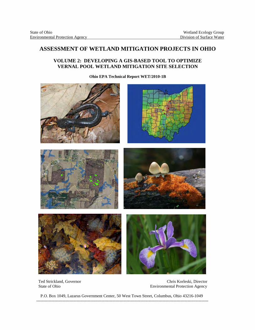
State of Ohio Wetland Ecology Group Environmental Protection Agency Division of Surface Water

ASSESSMENT OF WETLAND MITIGATION PROJECTS IN OHIO

VOLUME 2: DEVELOPING A GIS-BASED TOOL TO OPTIMIZE VERNAL POOL WETLAND MITIGATION SITE SELECTION

Ohio EPA Technical Report WET/2010-1B

Ted Strickland, Governor Chris Korleski, Director State of Ohio Environmental Protection Agency P.O. Box 1049, Lazarus Government Center, 50 West Town Street, Columbus, Ohio 43216-1049 ----------------------------------------------------------------------------------------------------------------------------

This page intentionally left blank.

ii

Appropriate Citation: Gara, B. D. and M. Micacchion. 2010. Assessment of wetland mitigation projects in Ohio. Volume 2: Developing a GIS-based tool to optimize vernal pool wetland mitigation site selection. Ohio EPA Technical Report WET/2010-1B. Ohio Environmental Protection Agency, Wetland Ecology Group, Division of Surface Water, Columbus, Ohio. This entire document can be downloaded from the web site of the Ohio EPA, Division of Surface Water: http://www.epa.state.oh.us/dsw/wetlands/WetlandEcologySection_reports.aspx

iii

ACKNOWLEDGMENTS

This study was funded under Wetland Program Development Grant CD00E09801-0 from U.S.

EPA Region 5. Thanks to Sue Elston, Catherine Garra, Lula Spruill, and Kristin Faulhaber (U.S.

EPA) for their technical and fiscal assistance. Special thanks to John Reinier, and Phil Renner,

Ohio EPA wetland interns in 2009 for their able assistance in field work and data entry and

analysis. Valuable assistance was provided by Martin Stapanian (USGS), Bill Schumacher (Ohio

EPA), and Pete Jackson (U.S. EPA Region V), who contributed their time and energy to several

of the vernal pool field assessments conducted during the summer of 2009. Their efforts were

most appreciated. Thanks also to Matt Fancher, David White, and Rich McClay (all of Ohio

EPA) for evaluating the technical aspects of the GIS model and to Bill Schumacher for collecting

and identifying all bryophyte specimens included in the study as a demonstration project.

iv

TABLE OF CONTENTS

ACKNOWLEDGMENTS ............................................................................................................ iv TABLE OF CONTENTS ............................................................................................................... v LIST OF TABLES ........................................................................................................................ vi LIST OF FIGURES ..................................................................................................................... vii ABSTRACT ................................................................................................................................ viii INTRODUCTION ......................................................................................................................... 1 METHODS .................................................................................................................................... 2 GIS MODEL TO QUANTIFY ECOLOGICAL INTEGRITY OF AREAS SURROUNDING NWI WETLANDS ................................................................................ 2 IDENTIFICATION OF POTENTIAL “HIGH QUALITY” VERNAL POOLS ................ 4 STUDY REGION AND SITE SELECTION FOR FIELD TESTING OF GIS MODEL ... 6 SAMPLING METHODS - LEVEL 2 RAPID ASSESSMENT .......................................... 6 SAMPLING METHODS - LEVEL 3 ASSESSMENT ....................................................... 6 CREATION OF A POTENTIAL VERNAL POOL RESTORATION GIS LAYER ......... 7 RESULTS AND DISCUSSION .................................................................................................... 9 LEVEL 1 IDENTIFICATION OF POTENTIAL “HIGH QUALITY” VERNAL POOLS .................................................................................................................. 9 MODEL RESULTS VS. CONDITION ASSESSMENTS OF NATURAL WETLANDS IN OHIO ....................................................................................................... 10 BRYOPHYTE DEMONSTRATION PROJECT RESULTS .............................................. 10 PRIORITIZING SITES FOR VERNAL POOL RESTORATION IN OHIO ..................... 10 STRENGTHS AND LIMITATIONS OF GIS MODEL ..................................................... 12 CONCLUSIONS.......................................................................................................................... 13 LITERATURE CITED ................................................................................................................ 14

v

LIST OF TABLES

Table 1. 1992 NLCD Land Use Categories corresponding LDI Coefficients ............................ 18 Table 2. 2001 NLCD Land Use Categories corresponding LDI Coefficients ............................ 19 Table 3. Metric scoring for NWI wetlands for areas from 0 to 100 meters of wetland boundary ........................................................................................................... 20 Table 4. Metric scoring for NWI wetlands for areas from 100 to 350 meters of wetland boundary ........................................................................................................... 21 Table 5. ORAM, VIBI, and AmphIBI scores for wetlands monitored in 2009 .......................... 22 Table 6. Bryophytes collected on September 30, 2009 from Alum Creek State Park ................ 23

vi

LIST OF FIGURES

Figure 1. OSIP true color orthophotography for Lawrence Woods State Nature Preserve, Hardin County, Ohio .................................................................................... 24 Figure 2. OSIP color infrared orthophotography for Lawrence Woods State Nature Preserve, Hardin County, Ohio ........................................................................ 25 Figure 3. Updated National Wetland Inventory polygons for Lawrence Woods State Nature Preserve, Hardin County, Ohio ............................................................... 26 Figure 4. Shrub swamp in Kokosing Wildlife Area (Knox County, Ohio) depicting inner (0 to 100 meters) and outer (100 to 350 meters) buffer zones........................... 27 Figure 5. Locations of 2009 field monitoring sites ..................................................................... 28 Figure 6. Potential high quality vernal pool locations in Ohio ................................................... 29 Figure 7. Potential high quality vernal pool locations in Ohio, color-coded by “quality” tiers. ......................................................................................................... 30 Figure 8. Wood Frog photograph from Fowler Woods State Nature Preserve, Richland County, Ohio ................................................................................................ 31 Figure 9. Spotted Salamander egg mass photograph from Alum Creek State Park, Delaware County, Ohio ...................................................................................... 32 Figure 10. Tiger Salamander photograph from Fowler Woods State Nature Preserve, Richland County, Ohio............................................................................... 33 Figure 11. Tuckerman’s Sedge photograph from Alum Creek State Park, Delaware County, Ohio ............................................................................................ 34 Figure 12. False Hop Sedge photograph from Alum Creek State Park, Delaware County, Ohio ............................................................................................ 35 Figure 13. Vernal pool restoration locations for Ohio ................................................................ 36 Figure 14. Vernal pool restoration locations for Ohio, color-coded by increasing “probability of success” levels .................................................................................... 37 Figure 15. Potential vernal pool restoration area surrounding Morris Woods State Nature Preserve, Licking County, Ohio ............................................................ 38

vii

ASSESSMENT OF WETLAND MITIGATION PROJECTS IN OHIO

VOLUME 2: DEVELOPING A GIS-BASED TOOL TO OPTMIZE VERNAL POOL WETLAND MITIGATION SITE SELECTION

Brian Gara Mick Micacchion

ABSTRACT

Wetland mitigation projects frequently result in habitat that is inferior in quality to the natural wetlands being impacted via permitted development activities. Better site selection has been identified as a primary factor for improving the resultant mitigation wetlands. Additionally, the replacement of ecological services provided by forested depressions known as “vernal pools” are rarely targeted as a component of wetland mitigation. These vernal pools represent critical breeding habitat for several species of sensitive amphibians, including Wood Frogs (Lithobates sylvaticus), Spotted Salamanders (Ambystoma maculatum), Marbled Salamanders (A. opacum), Jefferson Salamanders (A. jeffersonianum), Tiger Salamanders (A. tigrinum), and Four-toed Salamanders (Hemidactylium scutatum). Without adequate replacement of these resources, Ohio continues to experience a “net loss” of amphibian habitat, even if the overall amount of wetland acreage has been stabilized via the regulation of water resource impacts. A GIS-based model was developed to provide a tool for the regulated community could use to target sites specifically for vernal pool restoration. As most of these pond-breeding amphibians are known to travel very short distances (generally less than a few hundred meters) from the original vernal pools where they originate, one of the most important factors to consider is the proximity of the restoration site to existing amphibian breeding locations. A GIS layer of potential “high quality” vernal pools was developed using digital National Wetland Inventory (NWI) layer created by Ducks Unlimited for Ohio using high resolution true color and color infrared (CIR) aerial photography collected in 2006-2007. Each polygon on this GIS data layer was placed into one of six different categories based on their specific Cowardin classification. The six classes were: 1) forested, 2) scrub-shrub, 3) emergent, 4) open water, 5) aquatic bed, and 6) mudflat. Only polygons likely to meet wetland criteria as defined by the Army Corps of Engineers 1987 delineation manual were included in the analysis (those classified as forested, scrub-shrub, and emergent). Each of these identified 134,736 NWI wetlands was analyzed to estimate the integrity (i.e., ecological condition) of the landscape surrounding the wetland boundary: an “inner zone” (from edge of wetland to a distance of 100 meters) and an “outer zone” (from 100 to 350 meters beyond wetland edge). A series of 10 metrics was generated independently for the two zones surrounding the wetlands as follows:

1) Landscape Development Intensity (LDI) - using 1992 National Land Cover Dataset (NLCD) data; 2) Landscape Development Intensity (LDI) - using 2001 NLCD Data; 3) Percent Forested – using ancillary 2001 NLCD Forest Percent Cover data layer; 4) Percent Impervious Surface – using ancillary 2001 NLCD Impervious Surface data layer; 5) Percent “developed land” – subset of 2001 NLCD data layer; 6) Presence/Absence of State Listed Species – using ODNR Natural Heritage data layer; 7) Percent of area consisting of other NWI wetlands; 8) Length of transportation corridor per acre of buffer – using ODOT transportation GIS layers; 9) Percent of area consisting of forest on digital USGS 7.5 topographic maps (DRGs); 10) Change in forest from DRGs (“historic” forest) to most recent (2001 NLCD) forest layer.

Each of these metrics was given a score between 0 and 10 based on the distribution of the various parameter values within each wetland type, in each of the two zones (0 to 100 meters and 100 to 350

viii

meters from the wetland boundary). Therefore, a score of 0 to 100 was generated for each zone, indicating the predicted level of ecological integrity based on these ten land use parameters. A final score between 0 and 100 was assigned for each wetland by weighting the inner zone score twice as much as that of the outer zone (([inner zone score*0.67] + [outer zone score*0.33])). To test the strength of this model at identifying potential high quality vernal pools based on ecological integrity of the surrounding landscape, 26 forested or scrub-shrub wetlands which scored in the upper quartile of all NWI polygons were identified and sampled using Level 2 (Ohio Rapid Assessment for Wetlands [ORAM]) and/or Level 3 (Vegetation Index of Biotic Integrity [VIBI], Amphibian Index of Biotic Integrity [AmphIBI]) analysis tools. Based on the ORAM analysis, 60.9% (14 of 23) scored as Category 3 wetlands. 70% (7 of 10) of the wetlands assessed using VIBI, and 100% (11 of 11) of those assessed using the AmphIBI, scored within the Category 3 range, which represent wetlands considered to be in the best ecological condition. Additionally, a total of 4 wetlands in this study scored at the Category 3 level for all three of these field procedures. No wetlands identified by the model that were monitored in 2009 scored below the upper end of Category 2 using any of these analysis tools. A GIS procedure was then used to identify and classify vernal pool wetlands based on the overall NWI data layer. Only wetlands smaller than 2 acres in size and classified as “forested” or “scrub-shrub” (the types of natural wetlands used by pond-breeding amphibians) were included in the analysis. Additionally, any wetlands having more than 75% of its area composed of alluvial soils, as defined by NRCS and Ohio soil scientists, were precluded. Four levels of potential high quality vernal pools were selected from this subset of wetlands based on the following factors:

Tier 1 - Overall surrounding land use (inner and outer zone) score > 45 (upper 2 quartiles of entire NWI

layer); - > 50% “historically” forested (topo map forest layer) within inner zone; - > 50% forested (current 2001 forest layer) within inner zone.

Tier 2

- Overall surrounding land use score > 61 (upper quartile of entire NWI layer); - > 65% “historically” forested (topo map forest layer) within inner zone; - > 65% forested (current 2001 forest layer) within inner zone.

Tier 3

- Overall surrounding land use score > 61 (upper quartile of entire NWI layer); - > 80% “historically” forested (topo map forest layer) within inner zone; - > 80% forested (current 2001 forest layer) within inner zone; - > 50% “historically” forested (topo map forest layer) within outer zone; - > 50% forested (current 2001 forest layer) within outer zone.

Tier 4

- Overall surrounding land use score > 75 (upper quartile of entire NWI layer); - > 80% “historically” forested (topo map forest layer) within inner zone; - > 80% forested (current 2001 forest layer) within inner zone; - > 80% “historically” forested (topo map forest layer) within outer zone; - > 80% forested (current 2001 forest layer) within outer zone.

Using this approach, a total of 12,120 NWI wetlands fall into one of these 4 tiers (~9% of the total dataset). A GIS layer of potential vernal pool restoration sites was created by buffering each of these vernal pool polygons a distance of 500 meters. In cases where vernal pools were located less than 500 meters apart, all were included as a single conglomerated analysis area. A total 5,135 potential restoration

ix

areas were identified using this approach. These areas were further refined by selecting only those that had greater than 10% of the area in agricultural land use (based on 2001 NLCD data) and greater than 10% of the area historically was likely to have been wetland (using NRCS SSURGO hydric soils data). 3,034 areas met these criteria and were included on the final vernal pool restoration GIS layer. This data layer was subdivided based on the number of NWI wetlands identified as potential high quality vernal pools located within the analysis area and whether at least one of these vernal pools were categorized as “scrub-shrub,” thereby increasing the likelihood that the appropriate hydrologic regime to support amphibian breeding populations was present. The final layer of potential vernal pool restoration sites was categorized as follows: Level 1: 1 identified potential high quality vernal pool in restoration area; 0 scrub-shrub (1,204 sites); Level 2: 1 identified potential high quality vernal pool in buffer area; 1+ scrub-shrub (254 sites); Level 3: 2 to 4 identified potential high quality vernal pools in buffer area; 0 scrub-shrub (826 sites); Level 4: 2 to 4 identified potential high quality vernal pools in buffer area; 1+ scrub-shrub (318 sites); Level 5: 5+ identified potential high quality vernal pools in buffer area; 0 scrub-shrub (194 sites); Level 6: 5+ identified potential high quality vernal pools in buffer area; 1+ scrub-shrub (238 sites).

x

Introduction

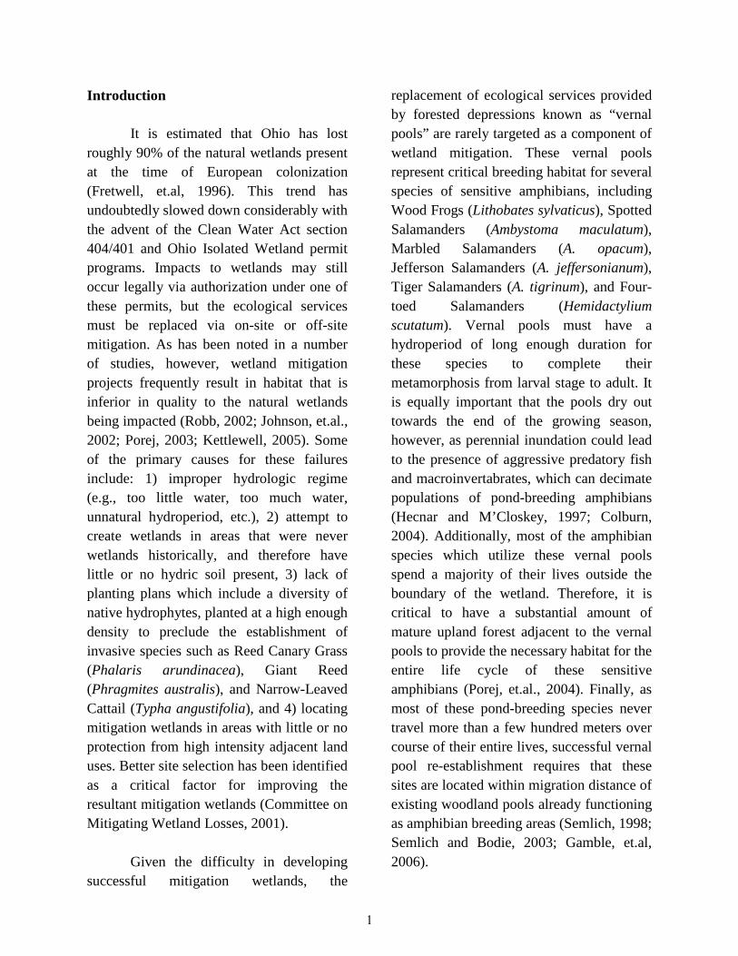
It is estimated that Ohio has lost roughly 90% of the natural wetlands present at the time of European colonization (Fretwell, et.al, 1996). This trend has undoubtedly slowed down considerably with the advent of the Clean Water Act section 404/401 and Ohio Isolated Wetland permit programs. Impacts to wetlands may still occur legally via authorization under one of these permits, but the ecological services must be replaced via on-site or off-site mitigation. As has been noted in a number of studies, however, wetland mitigation projects frequently result in habitat that is inferior in quality to the natural wetlands being impacted (Robb, 2002; Johnson, et.al., 2002; Porej, 2003; Kettlewell, 2005). Some of the primary causes for these failures include: 1) improper hydrologic regime (e.g., too little water, too much water, unnatural hydroperiod, etc.), 2) attempt to create wetlands in areas that were never wetlands historically, and therefore have little or no hydric soil present, 3) lack of planting plans which include a diversity of native hydrophytes, planted at a high enough density to preclude the establishment of invasive species such as Reed Canary Grass (Phalaris arundinacea), Giant Reed (Phragmites australis), and Narrow-Leaved Cattail (Typha angustifolia), and 4) locating mitigation wetlands in areas with little or no protection from high intensity adjacent land uses. Better site selection has been identified as a critical factor for improving the resultant mitigation wetlands (Committee on Mitigating Wetland Losses, 2001).

Given the difficulty in developing

successful mitigation wetlands, the

replacement of ecological services provided by forested depressions known as “vernal pools” are rarely targeted as a component of wetland mitigation. These vernal pools represent critical breeding habitat for several species of sensitive amphibians, including Wood Frogs (Lithobates sylvaticus), Spotted Salamanders (Ambystoma maculatum), Marbled Salamanders (A. opacum), Jefferson Salamanders (A. jeffersonianum), Tiger Salamanders (A. tigrinum), and Four-toed Salamanders (Hemidactylium scutatum). Vernal pools must have a hydroperiod of long enough duration for these species to complete their metamorphosis from larval stage to adult. It is equally important that the pools dry out towards the end of the growing season, however, as perennial inundation could lead to the presence of aggressive predatory fish and macroinvertabrates, which can decimate populations of pond-breeding amphibians (Hecnar and M’Closkey, 1997; Colburn, 2004). Additionally, most of the amphibian species which utilize these vernal pools spend a majority of their lives outside the boundary of the wetland. Therefore, it is critical to have a substantial amount of mature upland forest adjacent to the vernal pools to provide the necessary habitat for the entire life cycle of these sensitive amphibians (Porej, et.al., 2004). Finally, as most of these pond-breeding species never travel more than a few hundred meters over course of their entire lives, successful vernal pool re-establishment requires that these sites are located within migration distance of existing woodland pools already functioning as amphibian breeding areas (Semlich, 1998; Semlich and Bodie, 2003; Gamble, et.al, 2006).

1

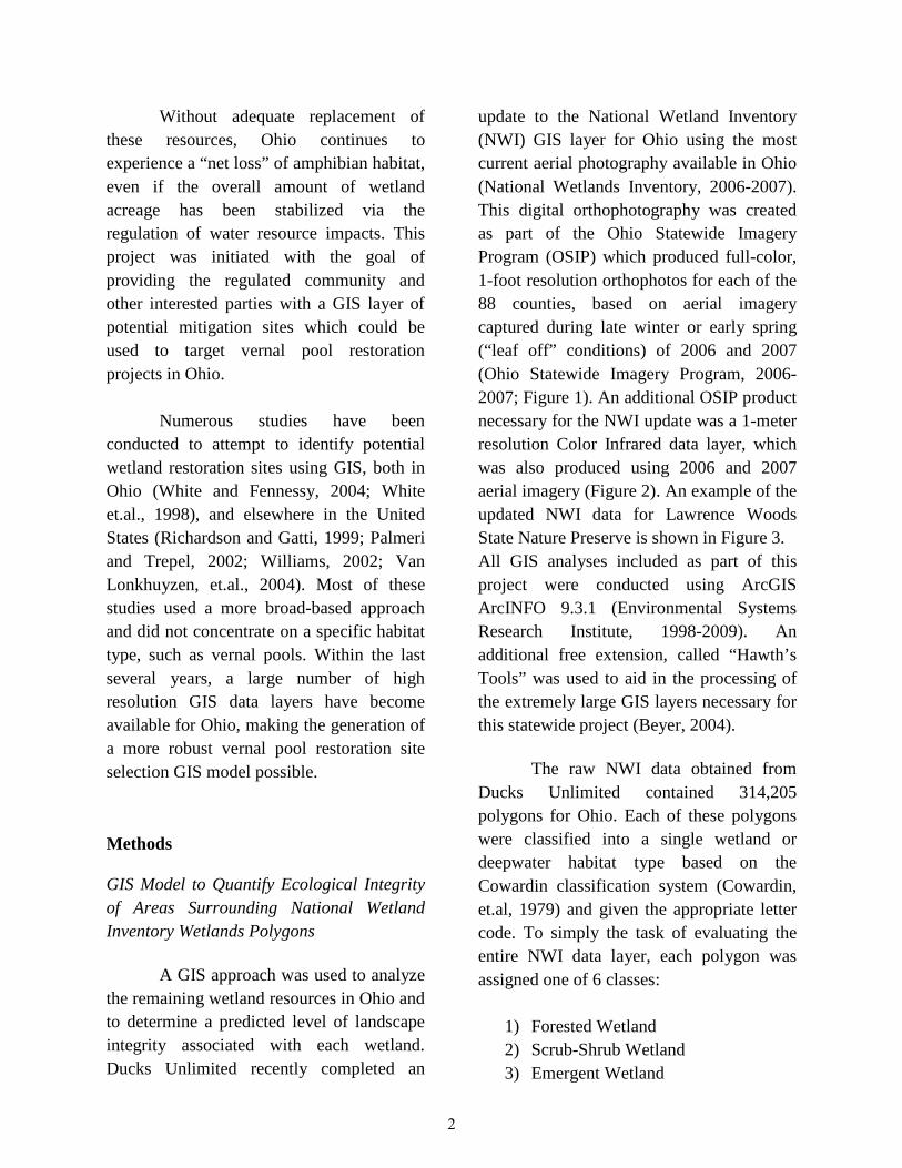
Without adequate replacement of these resources, Ohio continues to experience a “net loss” of amphibian habitat, even if the overall amount of wetland acreage has been stabilized via the regulation of water resource impacts. This project was initiated with the goal of providing the regulated community and other interested parties with a GIS layer of potential mitigation sites which could be used to target vernal pool restoration projects in Ohio.

Numerous studies have been

conducted to attempt to identify potential wetland restoration sites using GIS, both in Ohio (White and Fennessy, 2004; White et.al., 1998), and elsewhere in the United States (Richardson and Gatti, 1999; Palmeri and Trepel, 2002; Williams, 2002; Van Lonkhuyzen, et.al., 2004). Most of these studies used a more broad-based approach and did not concentrate on a specific habitat type, such as vernal pools. Within the last several years, a large number of high resolution GIS data layers have become available for Ohio, making the generation of a more robust vernal pool restoration site selection GIS model possible.

Methods GIS Model to Quantify Ecological Integrity of Areas Surrounding National Wetland Inventory Wetlands Polygons

A GIS approach was used to analyze the remaining wetland resources in Ohio and to determine a predicted level of landscape integrity associated with each wetland. Ducks Unlimited recently completed an

update to the National Wetland Inventory (NWI) GIS layer for Ohio using the most current aerial photography available in Ohio (National Wetlands Inventory, 2006-2007). This digital orthophotography was created as part of the Ohio Statewide Imagery Program (OSIP) which produced full-color, 1-foot resolution orthophotos for each of the 88 counties, based on aerial imagery captured during late winter or early spring (“leaf off” conditions) of 2006 and 2007 (Ohio Statewide Imagery Program, 2006-2007; Figure 1). An additional OSIP product necessary for the NWI update was a 1-meter resolution Color Infrared data layer, which was also produced using 2006 and 2007 aerial imagery (Figure 2). An example of the updated NWI data for Lawrence Woods State Nature Preserve is shown in Figure 3. All GIS analyses included as part of this project were conducted using ArcGIS ArcINFO 9.3.1 (Environmental Systems Research Institute, 1998-2009). An additional free extension, called “Hawth’s Tools” was used to aid in the processing of the extremely large GIS layers necessary for this statewide project (Beyer, 2004).

The raw NWI data obtained from Ducks Unlimited contained 314,205 polygons for Ohio. Each of these polygons were classified into a single wetland or deepwater habitat type based on the Cowardin classification system (Cowardin, et.al, 1979) and given the appropriate letter code. To simply the task of evaluating the entire NWI data layer, each polygon was assigned one of 6 classes:

1) Forested Wetland 2) Scrub-Shrub Wetland 3) Emergent Wetland

2

4) Open Water 5) Aquatic Bed 6) Mudflat

Only polygons likely to meet the

necessary criteria (forested, scrub-shrub, and emergent wetlands) to be considered a wetland based on the Army Corps of Engineers 1987 “Wetlands Delineation Manual” were included in this study (Environmental Laboratory, 1987). Eliminating the polygons not likely to meet wetland criteria (open water, aquatic bed, and mudflat), reduced the number of NWI polygons to be analyzed to 134, 736.

Each of these polygons was buffered two different distances using the buffer tool in ArcGIS 9.3.1 (ArcToolbox > Analysis Tools > Proximity > Buffer): 1) from the edge of the digital wetland polygon boundary to a distance of 100 meters (“inner zone”), and 2) from 100 to 350 meters away from the wetland boundary (“outer zone”) (Figure 4).

A series of 10 different metrics were

calculated for both the inner zone and outer zone for each wetland, by examining a number of different disturbance and stability parameters: 1) Landscape Development Intensity (LDI)

index using 1992 National Land Cover Dataset (NLCD) data for Ohio (Brown and Vivas, 2005; Vogelman et.al, 2001). The LDI is a means of assigning a “human disturbance” value using land use data, which allows areas to be evaluated along a gradient of disturbance based on the LDI score. In this study, the number of raster cells falling within a

wetland’s inner or outer zone for each 1992 NLCD land use category was multiplied by the associated LDI coefficient, as listed on Table 1. The sum total of all LDI/land use calculations was then divided by the total number of raster associated with each inner and outer zone area.

2) Landscape Development Intensity (LDI)

index using 2001 National Land Cover Dataset (NLCD) data for Ohio (Brown and Vivas, 2005; Homer et.al., 2004). The calculation is essentially the same, except the 2001 NLCD data has a few different land use categories and associated LDI coefficients (Table 2).

3) Percent Forested Area within the inner

and outer zones based on ancillary 2001 NLCD “Tree Canopy” raster dataset (Homer et.al, 2004; Huang et.al., 2003). Average percent forested cover per 30 meter by 30 meter pixel of zone area.

4) Percent Impervious Surface within the

inner and outer zones based on ancillary 2001 NLCD “Impervious” raster dataset (Homer et.al, 2004; Yang et.al., 2003). Average percent impervious surface per 30 meter by 30 meter pixel of zone area.

5) Percent “developed land” within inner

and outer zones surrounding each wetland (Homer et.al., 2004). Total number of 30 meter by 30 meters pixels classified as developed land (land use categories 21, 22, 23, or 24 in the 2001 NLCD Land Use dataset), divided by the total number of pixels comprising each zonal area.

3

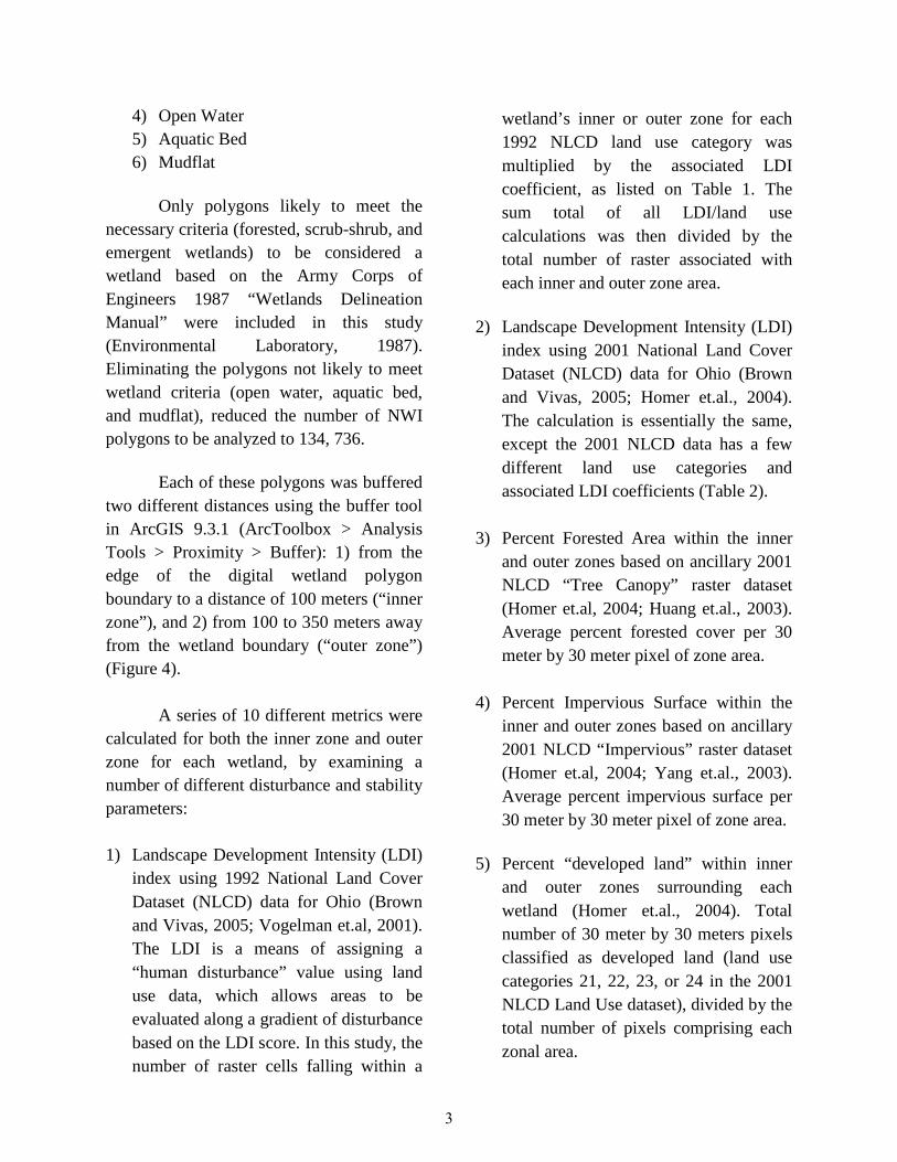
6) Presence/Absence of State Listed

Species within the inner and outer zones. Using the Ohio Department of Natural Resources “Heritage Database” (Ohio Division of Natural Areas and Preserves, 2008) one or more records of any species listed as “endangered” or “threatened” within either zone qualifies as “yes,” and receive a metric score of 10. The absence of any species having these designations would be marked as “no” and scored as 0.

7) Percent of area consisting of other NWI

wetlands (National Wetlands Inventory, 2006-2007). The inner and outer zone surrounding each wetland was compared to the statewide NWI GIS layer (only polygons listed as “emergent,” “scrub-shrub,” or “forested” were included in this analysis) to determine the percent of wetland habitat occurring within these areas.

8) Length of transportation corridor per

acre of inner and outer zone. Several Ohio Department of Transportation GIS layers (major roads, minor roads, local roads, and active railroads) were combined to generate this score (Ohio Department of Transportation, 2009).

9) Percent of “historic forest” within inner

and outer zones. The raster version of the USGS 7.5 minute topographic maps (“Digital Raster Graphics,” or DRGs) was processed to extract all forested areas as a separate GIS layer. As most of the source topographic maps used to create the DRGs in Ohio are generally

30 to 40 years old, this is the oldest source of information on forest resources available statewide.

10) “Forest Stability” within the two zones

surrounding each wetland. If an inner or outer zone consisted of least 50% “historic forest” and 50% forest based on the 2001 NLCD data layer, it would be given a score of 10 for the forest stability metric. Not meeting these criteria would score 0.

Each of these metrics was given a

score between 0 and 10 based on the distribution of the various parameter values within each wetland type (emergent, scrub-shrub, and forested), for both the inner and outer zone.

A complete breakdown of metric

scores based on these parameter ranges can be found in Tables 3 (inner zone) and 4 (outer zone). Each zone was given a score of 0 to 100 by summing the individual 10 metric scores. A final estimate of ecological integrity was generated for each emergent, scrub-shrub, and forested NWI wetland using the following formula: Final score for the wetland = (inner zone score * 0.67) + (outer zone score * 0.33) Identification of Potential “High Quality” Vernal Pools

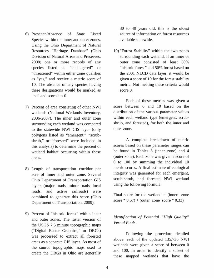
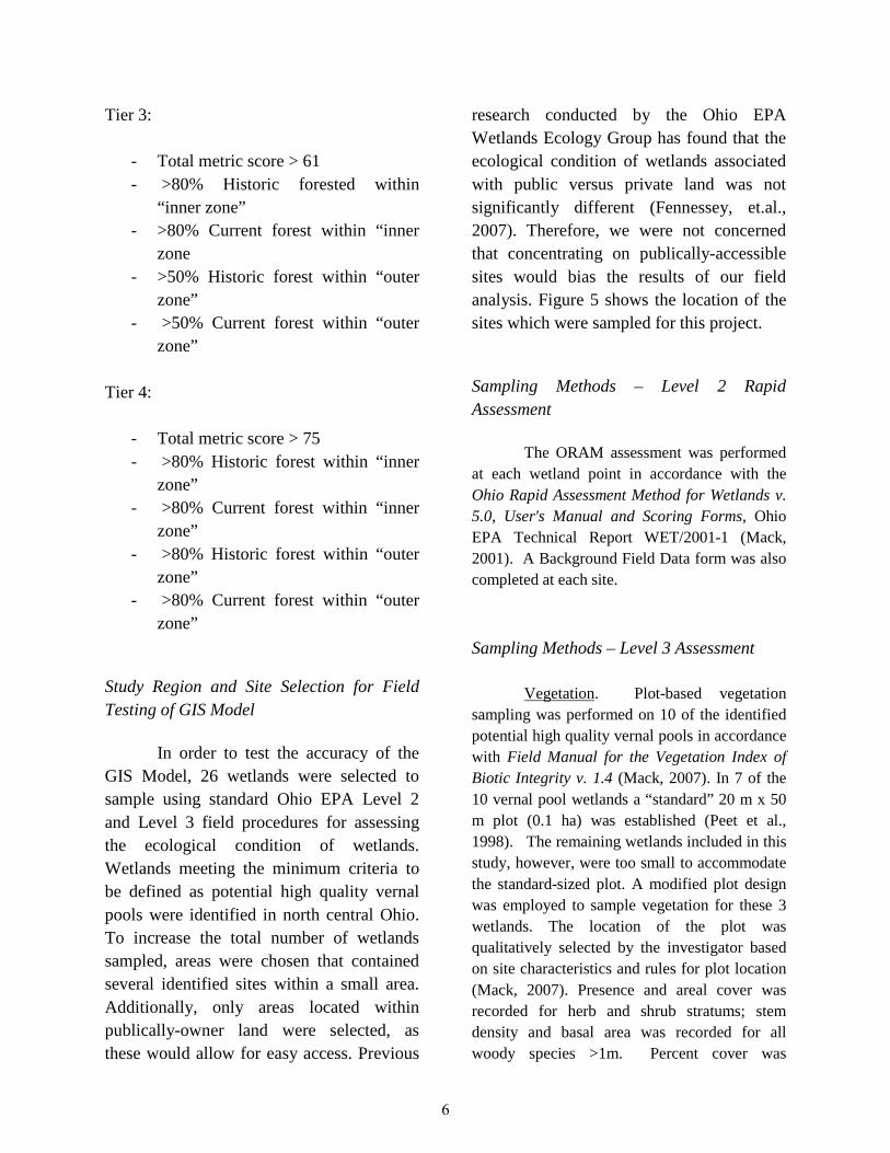
Following the procedure detailed above, each of the updated 135,736 NWI wetlands were given a score of between 0 and 100. In order to identify a subset of these mapped wetlands that have the

4

potential to support populations of pond-breeding amphibians, the following criteria were selected: 1) Only wetlands categorized as Forested

or Scrub-Shrub were included, as these were the most likely to have the characteristics typical of most Ohio vernal pools.

2) Wetlands having a total Level 1 score in the upper 2 quartiles of the entire NWI dataset, indicating a reasonable amount of ecological integrity of the areas surrounding each of these wetlands.

3) Only wetlands 2 acres in size or smaller

were selected. Based on data collected by the Ohio EPA Wetland Ecology Group, the vernal pools scoring better as amphibian breeding habitat were typically those that were smaller in size.

4) The amount of current forest within the inner zone surrounding the wetland is at least 50%.

5) The amount of historic forest (as defined

by the USGS topographic data) within the inner zone is also at least 50%.

6) The wetland does not occur on soils mapped as “alluvial” based on the NRCS Soil Survey Geographic (SSURGO) database (Soil Survey Staff, Natural Resources Conservation Service, United States Department of Agriculture, accessed 2009). A query was generated by the NRCS National Soils Database Manager (Paul Finnell, personal communication) to identify the soil map units likely to have developed under

typical overflow flooding conditions associated with rivers and major streams. This layer was refined further by input from Ohio EPA Soil Scientist Bill Schumacher, based on field experience with Ohio hydric soils (Bill Schumacher, personal communication). The hydrologic regime associated with these typical waterway flood events is not consistent with the typical vernal pool hydroperiod and ecology and is likely to negatively impact the ability of pond-breeding amphibians to reproduce successfully. Therefore, all wetlands having at least 70% of the mapped area occurring on an alluvial soil were precluded from the analysis.

The subset of wetlands meeting these

six criteria are considered to be potential high quality vernal pools. The GIS model was refined further to subdivide this group into four different “tiers” based on an increasing predicted level of ecological integrity. Tier 1:

- Total metric score > 45 - >50% Historic forested within

“inner zone” - >50% Current forest within “inner

zone” Tier 2:

- Total metric score > 61 (upper quartile of all NWI Level 1 scores)

- >65% Historic forested within “inner zone”

- >65% Current forest within “inner zone

5

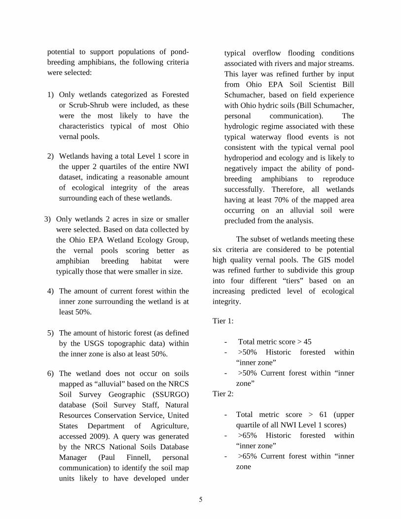
Tier 3:

- Total metric score > 61 - >80% Historic forested within

“inner zone” - >80% Current forest within “inner

zone - >50% Historic forest within “outer

zone” - >50% Current forest within “outer

zone” Tier 4:

- Total metric score > 75 - >80% Historic forest within “inner

zone” - >80% Current forest within “inner

zone” - >80% Historic forest within “outer

zone” - >80% Current forest within “outer

zone” Study Region and Site Selection for Field Testing of GIS Model

In order to test the accuracy of the GIS Model, 26 wetlands were selected to sample using standard Ohio EPA Level 2 and Level 3 field procedures for assessing the ecological condition of wetlands. Wetlands meeting the minimum criteria to be defined as potential high quality vernal pools were identified in north central Ohio. To increase the total number of wetlands sampled, areas were chosen that contained several identified sites within a small area. Additionally, only areas located within publically-owner land were selected, as these would allow for easy access. Previous

research conducted by the Ohio EPA Wetlands Ecology Group has found that the ecological condition of wetlands associated with public versus private land was not significantly different (Fennessey, et.al., 2007). Therefore, we were not concerned that concentrating on publically-accessible sites would bias the results of our field analysis. Figure 5 shows the location of the sites which were sampled for this project. Sampling Methods – Level 2 Rapid Assessment

The ORAM assessment was performed at each wetland point in accordance with the Ohio Rapid Assessment Method for Wetlands v. 5.0, User's Manual and Scoring Forms, Ohio EPA Technical Report WET/2001-1 (Mack, 2001). A Background Field Data form was also completed at each site. Sampling Methods – Level 3 Assessment

Vegetation. Plot-based vegetation sampling was performed on 10 of the identified potential high quality vernal pools in accordance with Field Manual for the Vegetation Index of Biotic Integrity v. 1.4 (Mack, 2007). In 7 of the 10 vernal pool wetlands a “standard” 20 m x 50 m plot (0.1 ha) was established (Peet et al., 1998). The remaining wetlands included in this study, however, were too small to accommodate the standard-sized plot. A modified plot design was employed to sample vegetation for these 3 wetlands. The location of the plot was qualitatively selected by the investigator based on site characteristics and rules for plot location (Mack, 2007). Presence and areal cover was recorded for herb and shrub stratums; stem density and basal area was recorded for all woody species >1m. Percent cover was

6

estimated using cover classes of Peet et al. (1998) (solitary/few, 0-1%, 1-2.5%, 2.5-5%, 5-10%, 10-25%, 25-50%, 50-75%, 75-90%, 90-95%, 95-99%). All woody stems >1 m tall were counted and placed into diameter classes (0-1 cm, 1- 2.5 cm, 2.5-5 cm, 5-10 cm, 10-15 cm, 20-25 cm, 25-30 cm, 30-35 cm, 35-40 cm) except for trees with diameters >40 cm which were individually measured and recorded. The midpoints of the cover and diameter classes were used in all analyses. Other data collected included various physical variables (e.g. % open water, depth to saturated soils, amount of coarse woody debris, etc.). A soil probe was used at the center of each plot to characterize the soil color and texture. Depth to saturation was also recorded.

Amphibians. Funnel traps were used in sampling the amphibians present in 10 of the identified potential high quality vernal pools. Sample methods followed the amphibian IBI protocols in Micacchion (2004). Funnel traps were constructed of aluminum window screen cylinders with fiberglass window screen funnels at each end. The funnel traps were similar in shape to commercially available minnow traps but with a smaller mesh-size. Ten funnel traps were placed evenly around the perimeter of the wetland and the trap location marked with flagging tape and numbered sequentially. Due to time limitations, only a single pass was conducted during the appropriate timeframe for each wetland included in this study. Many wetlands in central Ohio appeared to still be recovering from a drought period the previous year, and were very slow to fill with water. Traps were unbaited and left in the wetland for twenty-four hours in order to ensure unbiased sampling for species with diurnal and nocturnal activity patterns. Upon

retrieval, the traps were emptied by everting the funnel and shaking the contents into a white collection and sorting pan. Organisms that could be readily identified in the field (especially adult amphibians and larger and easily identified fish) were counted and released. The remaining organisms were transferred to wide-mouth one liter plastic bottles and preserved with 95% ethanol. Laboratory analysis of the preserved funnel trap contents was conducted to identify all larval amphibians (frog and toad tadpoles and salamander larvae) that had been collected in the field.

Bryophytes. A demonstration project was conducted to begin studying the potential of bryophytes as an indicator group for assessing wetland condition in Ohio. All recognized species of mosses and liverworts were collected from within an established VIBI plot for one of the high quality vernal pools included in this study (Alum Creek State Park – Africa Road). Each collected specimen was identified to species in the laboratory and an FQAI score was generated for the site using the coefficient of conservatism values assigned to each moss species in the “Floristic Quality Assessment Index (FQAI) for Vascular Plants and Mosses for the State of Ohio” (Andreas, Mack and McCormac, 2004). Creation of a Potential Vernal Pool Restoration GIS Layer

To define specific vernal pool restoration sites in Ohio, all NWI wetlands meeting the minimum criteria of potential high quality vernal pools were buffered a distance of 500 meters using the buffer tool

7

in ArcGIS 9.3.1 (ArcToolbox > Analysis Tools > Proximity > Buffer). This distance was chosen to eliminate areas that were clearly beyond the typical migration distance of most pond-breeding amphibian species (Semlich, 1998; Semlich and Bodie, 2003; Gamble, et.al, 2006). In cases of multiple potential high quality vernal pools located close to one another (i.e. less than 500 meters apart), the buffers were dissolved into a single polygon representing a discrete area to be analyzed for its restoration potential.

In addition to the proximity to vernal pools likely to be harboring populations of sensitive amphibian species, two additional factors were required for a buffer area to be considered a candidate for vernal pool restoration: 1) At least 10% of the overall area had to be defined as “historic wetland.” The NRCS SSURGO data layer for Ohio contains an attribute indicating the percent of hydric inclusion for each soil map unit (Soil Survey Staff, Natural Resources Conservation Service, United States Department of Agriculture, accessed 2009). The combined area of each soil type was summed for the buffer area and multiplied by the proportion of the soil consisting of hydric inclusions. The total wetland area was then summed and divided by the total area contained within each buffer area to estimate the percent of “historic wetland.” 2) At least 10% of the overall area also needed to be categorized as having an agricultural land use, according to the 2001 NLCD dataset (Homer et. al., 2004). The amount of agricultural land present was

quantified by tallying all cells consisting of one of the two NLCD agricultural land use types (pasture and row crops) and divided by the total number of cells contained within the buffer area.

Each buffer area meeting these minimum criteria was selected as a potential vernal pool restoration area. These sites were further refined by considering the total number of potential high quality vernal pools contained within and whether or not at least one of these wetlands were classified as scrub-shrub. It is assumed that the greater the number of high quality vernal pools present, the more likely one of them will have the appropriate habitat features to support populations of pond-breeding amphibians. It is also the experience of the Ohio EPA Wetland Ecology Group that NWI polygons classified as “scrub-shrub” which occur within forested areas are more likely to have the necessary hydroperiod to support these frog and salamander species than NWI polygons classified as “forested.” Therefore, each of the potential vernal pool restoration areas was placed into one of six levels, in which the scale indicates an increasing level of confidence that restoration potential exists: Level 1: 1 identified potential high quality vernal pool in restoration area; 0 scrub-shrub; Level 2: 1 identified potential high quality vernal pool in buffer area; 1+ scrub-shrub; Level 3: 2 to 4 identified potential high quality vernal pools in buffer area; 0 scrub-shrub; Level 4: 2 to 4 identified potential high quality vernal pools in buffer area; 1+ scrub-shrub;

8

Level 5: 5+ identified potential high quality vernal pools in buffer area; 0 scrub-shrub; Level 6: 5+ identified potential high quality vernal pools in buffer area; 1+ scrub-shrub. Results and discussion Level 1 Identification of Potential “High Quality” Vernal Pools

The updated National Wetland Inventory (NWI) layer created by Ducks Unlimited for Ohio (National Wetlands Inventory, 2006-2007) consists of 314,205 polygons. Removing all NWI polygons classified as “open water,” “aquatic bed,” and “mudflat” reduced the total number of polygons likely to meet wetland criteria (classified as “forested,” “scrub-shrub,” and “emergent”) to 134,736. The Level 1 analysis conducted on each to identify the potential existing high quality vernal pools further eliminated most NWI wetlands. The final result was a total of 12,120 polygons meeting the minimum criteria to be considered potential high quality vernal pools (Figure 6). The refinement of these wetlands into an increasing scale of “quality” tiers, as discussed above, resulted in the following number in each tier (Figure 7): Tier 1: 6,025 wetlands Tier 2: 4,591 wetlands Tier 3: 1,184 wetlands Tier 4: 320 wetlands

The final GIS layer and associated metadata containing all NWI wetland boundaries along with attributes for all

metrics included in this analysis can be downloaded from the following location: ftp://ftp-gis.epa.state.oh.us/gisdepot/gisdata/dsw/wetlands/NWI_wetlands_with_landscape_intensity_attributes.zip

While the distribution of these potential high quality vernal pools covers the entire state, some patterns are evident. Very few of these vernal pool wetlands were identified in the area of Ohio covered by the Huron/Erie Lake Plains Ecoregion, relative to the rest of the state. Historically, this is the location of the original “Great Black Swamp” in northwest Ohio (Katz, 1955). The area has been almost completely drained, and is now one of the most productive agricultural areas of the state. Most of wetlands identified as potential high quality vernal pools in this ecoregion are clustered in an area of sand deposits located just west of Toledo, referred to as the “Oak Openings.” The Oak Openings area is considered to be one of the most diverse biotic areas of the state (Brewer and Vankat, 2004). Any of these identified resources not occurring on one of the several existing parks and nature preserves in the region should be investigated.

A substantial number of potential high quality vernal pools are distributed in a band running roughly east west across the northern 3rd of the state. Most of the wetlands that have been classified as “Tier 4” are located in the unglaciated area of Ohio, which contains the most substantial amount of remaining forest habitat in the state.

9

Model Results vs. Ecological Condition Assessments of Natural Wetlands in Ohio

A total of 26 wetlands identified as being potential high quality vernal pools were monitored using Level 2 and Level 3 ecological assessment techniques. Results of this field work are recorded in Table 5. Of the 23 wetlands in which an ORAM evaluation was conducted, a total of 14 received a score greater than 60 (61%), which classifies each of these wetlands as either Category 3 or in the “gray zone” between Category 2 and Category 3. The Vegetation Index of Biotic Integrity (VIBI) was performed on a total of 10 wetlands in this study, and 7 (70%) scored as Category 3 wetlands. Of the wetlands that did not score in the Category 3 range for ORAM or VIBI, none scored lower than Category 2. A detailed assessment of the amphibian community (AmphIBI) was conducted on 11 of these identified potential high quality vernal pools, and all of them (100%) scored as Category 3 wetlands. Four wetlands included in this study (Alum Creek SP Beach 1, Alum Creek SP Africa Road 1, Killdeer Plains WA East 3, and Kokosing WA 1) scored as Category 3 wetlands for all three field assessment procedures. These vernal pools could truly be considered among the “best of the best.”

Several sensitive amphibian species were recorded at one or more of these sites, including Wood Frog (Lithobates sylvaticus) (Figure 8), Spotted Salamander (Ambystoma maculatum) (Figure 9), Tiger Salamander (Ambystoma tigrinum) (Figure 10), Jefferson Salamander (Ambystoma jeffersonianum), and Red-Spotted Newt (Notophtalmus

viridescens). Additionally, a number of sensitive plant species were encountered during the course of the 2009 field season, while conducting surveys for this research, including Tuckerman’s Sedge (Carex tuckermanii) (Figure 11), False Hop Sedge (Carex lupuliformis) (Figure 12), Drooping Sedge (Carex prasina), Royal Fern (Osmunda regalis), and Crested Fern (Dryopteris cristata). The results of this field verification study suggests that the GIS model created to assess the condition of the landscape surrounding the NWI wetlands is able to identify vernal pools that are in good to excellent ecological condition. Bryophyte demonstration project results

A total of 17 species of mosses were collected and identified to species level from the Alum Creek State Park Africa Road 1 vernal pool site (Table 6). The final Moss FQAI score calculated for the site was 13.82. The main purpose for conducting this demonstration project was to explore the potential viability of using this taxonomic group for assessing the ecological condition of wetlands in Ohio. In the future, additional sites representing a wide range of condition levels will be sampled using the moss collection protocols developed during this preliminary study. Prioritizing Sites for Vernal Pool Restoration in Ohio

A total of 3,034 potential vernal pool restoration sites were identified across Ohio (Figure 13). Notable patterns are evident when these data are compared with the

10

Level 3 ecoregion boundaries for Ohio (Woods, et.al., 1998). A vast majority of these sites are located in the Eastern Corn Belt Plains and Erie/Ontario Drift and Lake Plain ecoregions in Ohio. Very few sites exist in Huron/Erie Lake Plains ecoregion, with the exception of the Oak Openings area. Most of Southeast Ohio is covered by the Western Alleghany Plateau ecoregion. Even though several wetlands were identified in this ecoregion that meet the criteria of potential high quality vernal pool and are expected to indeed meet that standard, very few vernal pool restoration sites were identified in the Western Alleghany Plateau ecoregion. This is probably due to the general lack of historic wetland habitat along with the relative paucity of agricultural land use in this area of the state.

These 3,034 potential restoration sites were refined into 6 different levels based on the total number of potential high quality vernal pools contained within the 500 meter buffer, and whether or not any of these are classified as “scrub-shrub” (Figure 14). Increasing level numbers are expected to correspond with the increasing likelihood that at least one of the identified existing vernal pools will contain pond-breeding amphibians, and therefore represent the “source” for population expansion of these sensitive species within a given restoration site. The total numbers of restoration sites based on these levels are as follows: Level 1: 1 HQ Vernal Pool; 0 Scrub-Shrub - N = 1,204 sites Level 2: 1 HQ Vernal Pool; 1 Scrub-Shrub N = 254 sites

Level 3: 2-4 HQ Vernal Pools; 0 Scrub- Shrub – N = 826 sites Level 4: 2-4 HQ Vernal Pools; 1+ Scrub- Shrub – N = 318 sites Level 5: 5+ HQ Vernal Pools; 0 Scrub- Shrub – N = 194 sites Level 6: 5+ HQ Vernal Pools; 1+ Scrub- Shrub – N = 238 sites

The final GIS layer and associated metadata containing all 3,034 identified vernal pool restoration locations along with the associated restoration levels described above can be downloaded from: ftp://ftp-gis.epa.state.oh.us/gisdepot/gisdata/dsw/wetlands/Potential_Vernal_Pool_Restoration_Sites.zip

Most of these potential vernal pool restoration sites are concentrated in west central Ohio and in the far northeastern corner of the state. The border between the Eastern Corn Belt Plains and Erie/Ontario Drift and Lake Plain ecoregions represents the largest concentration of sites classified as level 6, which are presumably the areas most likely to provide successful restoration opportunities. Another significant area containing these level 6 sites is located in Ashtabula, Trumbull, and Mahoning Counties.

An example of one level 6 restoration area is included as Figure 15. This site encompasses Morris Woods State Nature Preserve in Licking County, Ohio.

11

As can be seen in this example, the intent of this project is to identify specific areas surrounding existing high quality resources that have the potential to expand the habitat for pond-breeding amphibians and, if possible, provide new migration corridors between existing vernal pools. The intact, functioning vernal pool/upland forest complex would be protected, with no habitat manipulation necessary. Surrounding these areas, agricultural lands consisting of predominantly hydric soil map units would be expected to be the locations for restored vernal pools. Additional areas of non-hydric soil surrounding these restored pools should be targeted for the re-establishment of upland forest as a necessary component of the overall site development. Strengths and Limitations of GIS Model

The main purpose of developing this GIS model was to predict the locations of high quality vernal pool wetlands, which could serve as the “source” of amphibians for wetland restoration projects targeting the habitat of these sensitive species. While a total score was generated for all NWI wetlands classified as forested, scrub-shrub, and emergent. Field monitoring was only conducted on wetlands meeting the specific criteria to be considered potential high quality vernal pools. Much more testing of natural wetlands would need to be done to determine if this model is actually valid for all wetland types, over the full range of human disturbance that was quantified using this Level 1 analysis.

Several potential sources of error should also be considered. All GIS data

contains a standard level of “acceptable” error, depending on the resolution of the data layer and the quality of the instruments used to capture the information via remote sensing technology. The starting point of this analysis was the creation of an updated NWI layer for Ohio. The assumption inherent in this Level 1 analysis is that these boundaries are “correct.” If, for whatever reason, wetland polygons are inaccurately defined, the subsequent analysis of areas surrounding these wetlands will also be flawed. It is expected that in most cases, the NWI wetland boundaries are reasonably accurate, but in all cases, any planning decisions made based on this study must be field verified to confirm the accuracy of the assessment.

Another potential source of error relates to the fact that all GIS layers represent a “snapshot in time.” As land use changes, sometimes quite rapidly in some areas of the state, these layers may no longer represent the condition of the landscape. Wetlands may be filled, agricultural land may become a housing subdivision, and new roads may be built. Therefore, the resultant GIS layers derived from this project will gradually become outdated as Ohio’s landscape changes. Although no updates are currently planned, it would be beneficial to regularly update the information associated with this study, including the wetland boundary and land use layers included in the Level 1 analysis.

The benefit of using this Level 1 GIS analysis tool is that it allows us to predict with a reasonable amount of accuracy locations that may be suitable to the re-establishment of vernal pools. It provides a

12

means for identifying specific locations which can then be investigated more thoroughly using standard Ohio EPA wetland field monitoring procedures. It is not intended that any GIS data created as part of this study be used as a surrogate for the more detailed Level 2 (e.g., ORAM) or Level 3 (e.g., VIBI, AmphIBI, etc.) analyses. Conclusions

The abundance of recently-generated, high quality GIS data for Ohio has provided the necessary tools for developing a robust Level 1 analysis of wetlands. This study focused on using a GIS model to identify existing high quality vernal pools along with potential restoration areas surrounding these resources. It must be emphasized that while field-testing of the model provided strong evidence that the GIS model can identify existing high quality vernal pools with a reasonable degree of statistical confidence, it is expected that field verification using more rigorous Level 2 and Level 3 procedures will always be necessary to verify that a given site is indeed appropriate for vernal pool restoration. This Level 1 GIS model does allow for a consistent statewide analysis which would otherwise not be possible via on-the-ground surveying. It also provides a cost-effective approach for selecting potential restoration sites and to target specific areas for monitoring using more intensive ecological assessment tools.

It is expected that as wetland professionals begin using this tool on a statewide basis, the model will need to be

refined as new field assessments are conducted and compared to the Level 1 results. In the future, the Ohio EPA Wetland Ecology Group will be running this model on wetlands in which a more accurate boundary is delineated using sub-meter accuracy GPS in the field. This will allow for a more rigorous statistical analysis of the correlation between ecological condition and landscape-level disturbance. In this manner it can be determined if the model is capable of accurately predicting wetland condition across a broad range of hydrogeomorphic and plant community classes.

13

Literature Cited

Andreas, B.K., J.J. Mack, and J.S. McCormac. 2004. Foristic quality assessment index (FQAI) for vascular plants and mosses for the State of Ohio. Ohio Environmental Protection Agency, Division of Surface Water, Wetland Ecology Group, Columbus, Ohio. 219 p. Beyer, H. L. 2004. Hawth's Analysis Tools for ArcGIS. Available at http://www.spatialecology.com/htools. Brewer, Lawrence G. and John L. Vankat. 2004. Description of the Vegetation of the Oak Openings or Northwestern Ohio at the Time of Eur-American Settlement. Ohio Journal of Science. Vol. 104 (4): 76-85. Brown, Mark T. and M. Benjamin Vivas. 2005. A Landscape Development Intensity Index. Environmental Monitoring and Assessment, vol. 101 (1-3), pp. 289-309. Colburn, E. 2004. Vernal Pools: Natural History and Conservation. The McDonald and Woodward Publishing Co., Blacksburg, Virginia. 426 pp. Committee on Mitigating Wetland Losses, Board on Environmental Studies and Toxicology, Water Science and Technology Board, National Research Council. 2001. Compensating for wetland losses under the Clean Water Act. NATIONAL ACADEMY PRESS, Washington, D.C. 322 p. Cowardin, L.M., V. Carter, F.C. Golet, E.T. LaRoe. 1979. Classification of wetlands and deepwater habitats of the United States. U.S. Department of the Interior, Fish and

Wildlife Service, Washington, D.C. Jamestown, ND: Northern Prairie Wildlife Research Center Home Page. http://www.npwrc.usgs.gov/resource/1998/classwet/classwet.htm (Version04DEC98). Environmental Laboratory. 1987. Corps of Engineers Wetlands Delineation Manual, Technical Report Y-87-1. U.S. Army Corps of Engineers, Vicksburg, MS. Environmental Systems Research Institute. ArcGIS: Release 9.3.1 [software]. Redlands, California: Environmental Systems Research Institute, 1999-2009. Fennessy, M.S., M.A. Gray, and R.D. Lopez. 1998a. An ecological assessment of wetlands using reference sites Volume 1: Final Report to U.S. Environmental Protection Agency for Grant CD99576. Ohio Environmental Protection Agency, Division of Surface Water, Wetlands Unit, Columbus, Ohio. 153 p. + appendices. Fennessy, M.S., R. Geho. B. Elfritz, and R. Lopez. 1998b. testing the floristic quality assessment index as an indicator of riparian wetland disturbance. Final Report to U.S. Environmental Protection Agency for Grant CD995927. Wetlands Unit, Division of Surface Water, 34 p. + appendices. Fennessy, M. S., J. J. Mack, E. Deimeke, M. T. Sullivan, J. Bishop, M. Cohen, M. Micacchion and M. Knapp. 2007. Assessment of wetlands in the Cuyahoga River watershed of northeast Ohio. Ohio EPA Technical Report WET/2007-4. Ohio Environmental Protection Agency, Division of Surface Water, Wetland Ecology Group, Columbus, Ohio.

14

Fretwell, J.D., Williams, J.S., and Redman, P.J., 1996. National water summary on wetland resources: U.S. Geological Survey Water-Supply Paper 2425. Gamble, Lloyd R., K. McGarigal, C.L. Jenkins, and B.C. Timm. 2006. Limitations of regulated “buffer zones” for the conservation of marbled salamanders. Wetlands, Vol. 26 (2), pp. 298-306. Hecnar, S.J. and R.T. M’Closkey. 1997. The effects of predatory fish on amphibian species richness and distribution. Diological Conservation 79, pp. 123-131. Homer, C. C. Huang, L. Yang, B. Wylie and M. Coan. 2004. Development of a 2001 National Landcover Database for the United States. Photogrammetric Engineering and Remote Sensing, Vol. 70, No. 7, July 2004, pp. 829-840. Huang, C., Homer, C., and L. Yang. 2003, Regional forest land cover characterization using Landsat type data, in Wulder, M., and Franklin, S., eds., Methods and Applications for Remote Sensing of Forests: Concepts and Case Studies, Kluwer Academic Publishers, p. 389-410. Kaatz, Martin R. 1955. The Black Swamp: A study in Historical Geography. Annals of the Association of American Geographers. Vol. 45, No. 1, pp. 1-35. Kettlewell, Chad. 2005. An inventory of Ohio wetland compensatory mitigation – Part 2. Ohio Environmental Protection Agency, Division of Surface Water, Wetland Ecology Group, Final Report to

U.S. EPA Grant No. CD97576201-0, Columbus, OH. Lopez, R.D. and M.S. Fennessy. 2002. Testing the floristic quality assessment index as an indicator of wetland condition. Ecological Applications 12(2):487-497. Mack, J.J. 2001. Ohio Rapid Assessment Method for Wetlands, Manual for Using Version 5.0. Ohio EPA Technical Bulletin WET2001-1. Ohio Environmental Protection Agency, Division of Surface Water, 401 Wetland Ecology Unit, Columbus, Ohio. Mack, J.J. 2007. Integrated Wetland Assessment Program. Part 9: Field manual for the Vegetation Index of Biotic Integrity v. 1.4. Ohio EPA Technical Report WET/2007-6. Ohio Environmental Protection Agency, Wetland Ecology Group, Division of Surface Water, Columbus, Ohio. Micacchion, M. 2004. Integrated wetland assessment program. Part 7: amphibian index of biotic integrity (AmphIBI) for Ohio wetlands. Ohio EPA Technical Report WET/2004-7. Ohio Environmental Protection Agency, Division of Surface Water, Wetland Ecology Group, Columbus, Ohio. National Wetlands Inventory (NWI) [GIS database], U.S. Fish and Wildlife Service, Updated by Ducks Unlimited, Inc., 2006-2007. Ohio Department of Transportation [GIS data]. 2009. Available from: http://www.dot.state.oh.us/divisions/transsys

15

dev/innovation/prod_services/esridwnloads/pages/default.aspx Ohio Division of Natural Areas and Preserves. 2008. Rare native Ohio plants: 2008-09 status list. Ohio Department of Natural Resources, Columbus, OH. 28 pp. Ohio Statewide Imagery Program (OSIP). 2006-2007. Ohio Office of Information Technology, Ohio Geographically Referenced Information Program (OGRIP). http://ogrip.oit.ohio.gov/. Palmeri, L. and M. Trepel. 2002. A GIS-based score system for siting and sizing of created or restored wetlands: Two case studies. Water Resources Management 16: 307-328. Peet, Robert K., Thomas R. Wentworth, and Peter S. White. 1998. A flexible, multipurpose method for recording vegetation composition and structure. Castanea 63(3): 262-274 Porej, D. 2003. An inventory of Ohio wetland compensatory mitigation. Ohio Environmental Protection Agency, Division of Surface Water, Wetland Ecology Group, Final Report to U.S. EPA Grant No. CD97576201-0, Columbus, OH. Porej, D., M. Micacchion and T. E. Hetherington. 2004. Core Terrestial Habitat for Conservation of Local Populations of Salamanders and Wood Frogs in Agricultural Landscapes. Biological Conservation 120:399-409. Richardson, M.S. and R.C. Gatti. 1999. Prioritizing wetland restoration activity

within a Wisconsin watershed using GIS modeling. Journal of Soil and Water Conservation 54: 537-542. Robb, James. 2002. Assessing Indiana compensatory mitigation sites to aid in establishing mitigation ratios. Wetlands 22(2): 435-440. Semlitsch, R. D. 1998. Biological Delineation of Terrestrial Buffer Zones for Pond-Breeding Salamanders. Biological Conservation 12(5):1113-1119. Semlitsch, R.D. and J.R. Bodie. 2003. Biological Criteria for Buffer Zones around Wetlands and Riparian Habitats for Amphibians and Reptiles. Biological Conservation 17(5):1219-1228. Soil Survey Staff, Natural Resources Conservation Service, United States Department of Agriculture. Soil surveys for each Ohio County available online from http://soildatamart.nrcs.usda.gov/Survey.aspx?State=OH [Accessed 2009]. Van Lonkhuyzen, R.A., K.E. Lagory, J.A. Kuiper. 2004. Modeling the suitability of potential wetland mitigation sites with a geographic information system. Environmental Management 33(3): pp. 368-375. Vogelmann, J.E., S.M. Howard, L. Yang, C. R. Larson, B. K. Wylie, and J. N. Van Driel, 2001, Completion of the 1990’s National Land Cover Data Set for the conterminous United States, Photogrammetric Engineering and Remote Sensing 67:650-662.

16

White, D., S. Fennessy, and A. Engelmann. 1998. The Cuyahoga watershed demonstration project for the identification of wetland restoration sites. Ohio EPA final report to the US Environmental Protection Agency – Region V. White, D. and S. Fennessy. 2005. Modeling the suitability of wetland restoration potential at the watershed scale. Ecological Engineering 24 (2005): pp. 359-377. Williams, K. B. 2002. The potential wetland restoration and enhancement site identification procedure: a geographic information system for targeting wetland restoration and enhancement. North Carolina Division of Coastal Management, Department of Environment and Natural Resources. Yang, L., C. Huang, C. Homer, B. Wylie and M. Coan. 2003. An approach for mapping large-area impervious surfaces: Synergistic use of Landsat 7 ETM+ and high spatial resolution imagery. Canadian Journal of Remote Sensing, Vol. 29, No. 2, pp.230-240. Woods, A. J., J. M. Omernik, C. S. Brockman, T. D. Gerber, W. D. Hosteter, and S. H. Azevedo, 1998. Ecoregions of Indiana and Ohio (Map) and Supplementary text.

17

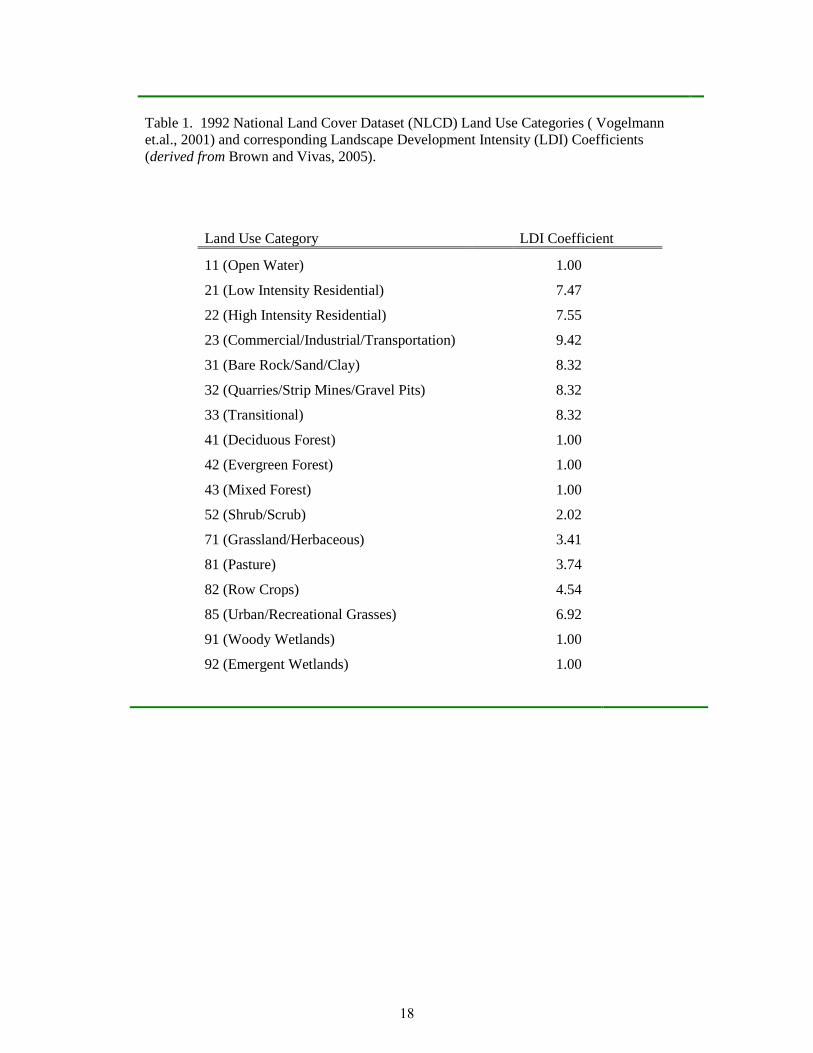
Table 1. 1992 National Land Cover Dataset (NLCD) Land Use Categories ( Vogelmann et.al., 2001) and corresponding Landscape Development Intensity (LDI) Coefficients (derived from Brown and Vivas, 2005).

Land Use Category LDI Coefficient

11 (Open Water) 1.00

21 (Low Intensity Residential) 7.47

22 (High Intensity Residential) 7.55

23 (Commercial/Industrial/Transportation) 9.42

31 (Bare Rock/Sand/Clay) 8.32

32 (Quarries/Strip Mines/Gravel Pits) 8.32

33 (Transitional) 8.32

41 (Deciduous Forest) 1.00

42 (Evergreen Forest) 1.00

43 (Mixed Forest) 1.00

52 (Shrub/Scrub) 2.02

71 (Grassland/Herbaceous) 3.41

81 (Pasture) 3.74

82 (Row Crops) 4.54

85 (Urban/Recreational Grasses) 6.92

91 (Woody Wetlands) 1.00

92 (Emergent Wetlands) 1.00

18

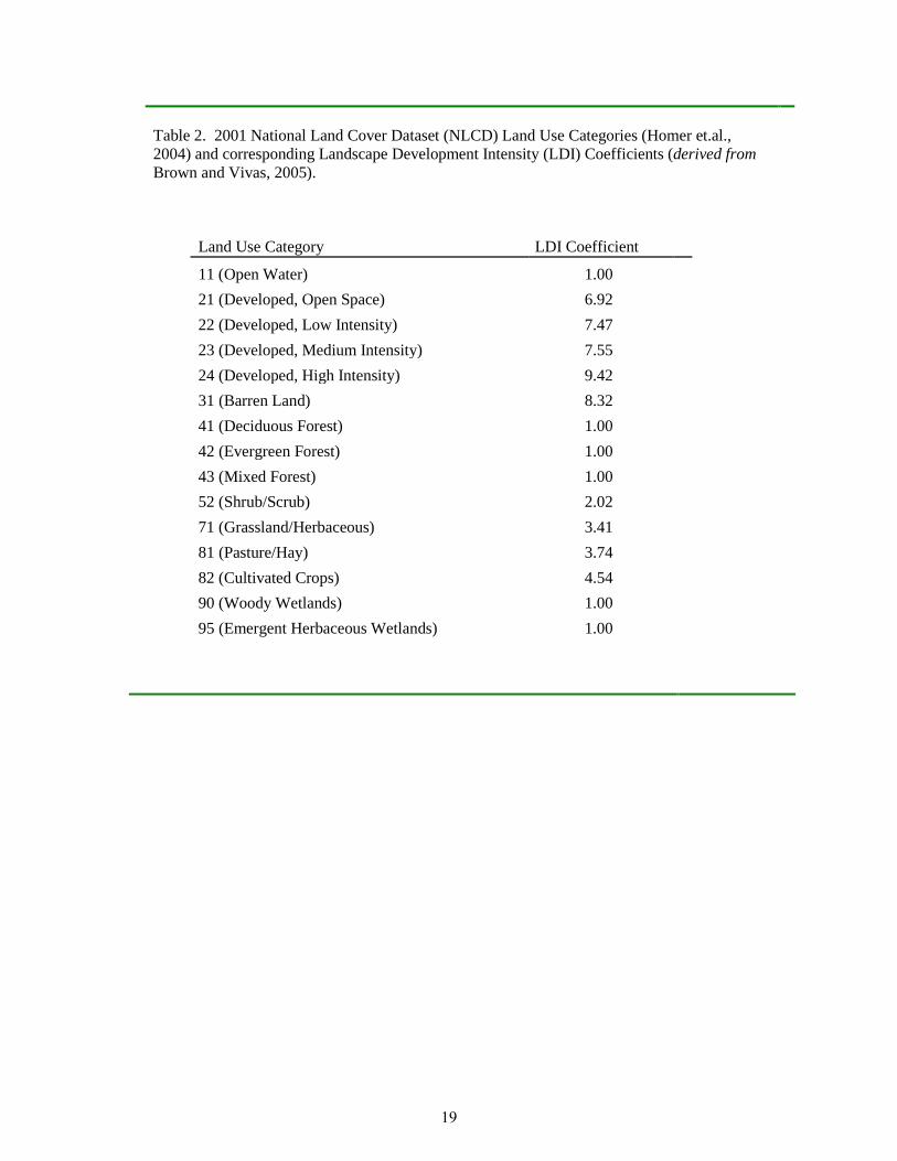
Table 2. 2001 National Land Cover Dataset (NLCD) Land Use Categories (Homer et.al., 2004) and corresponding Landscape Development Intensity (LDI) Coefficients (derived from Brown and Vivas, 2005).

Land Use Category LDI Coefficient

11 (Open Water) 1.00 21 (Developed, Open Space) 6.92 22 (Developed, Low Intensity) 7.47 23 (Developed, Medium Intensity) 7.55 24 (Developed, High Intensity) 9.42 31 (Barren Land) 8.32 41 (Deciduous Forest) 1.00 42 (Evergreen Forest) 1.00 43 (Mixed Forest) 1.00 52 (Shrub/Scrub) 2.02 71 (Grassland/Herbaceous) 3.41 81 (Pasture/Hay) 3.74 82 (Cultivated Crops) 4.54 90 (Woody Wetlands) 1.00 95 (Emergent Herbaceous Wetlands) 1.00

19

Table 3. Metric scoring for Emergent, Forested, and Scrub-Shrub NWI wetlands for areas from 0 to 100 meters of wetland boundary.

Paremeter

Emergent Wetlands (N = 56, 983 )

Forested Wetlands (N = 55, 650 )

Scrub-Shrub Wetlands (N = 22,103 )

1) LDI Index (1992) Metric Score = 0 Metric Score = 3 Metric Score = 7 Metric Score = 10

4.277313 – 9.420000 (N = 14,244) 3.628077 – 4.277200 (N = 14,245) 2.644222 – 3.628000 (N = 14,246) 1.000000 – 2.644000 (N = 14,248)

3.074536 – 8.630625 (N = 13,913) 2.266646 – 3.074444 (N = 13,911) 1.525970 – 2.266552 (N = 13,912) 1.000000 – 1.525916 (N = 13,914)

3.238929 – 9.160923 (N = 5,525) 2.320761 – 3.238675 (N = 5,526) 1.534634 – 2.320595 (N = 5,529) 1.000000 – 1.534621 (N = 5,523)

2) LDI Index (2001) Metric Score = 0 Metric Score = 3 Metric Score = 7 Metric Score = 10

4.540098– 9.356610 (N = 10,008) 3.861078 – 4.540000 (N = 18,483) 2.745000 – 3.861035 (N = 14,245) 1.000000 – 2.744348 (N = 14,247)

3.309558 – 8.421539 (N = 13,909) 2.387529 – 3.309091 (N = 13,910) 1.566471 – 2.387500 (N = 13,908) 1.000000 – 1.566400 (N = 13,923)

3.590612 – 9.420000 (N = 5,526) 2.537434 – 3.590244 (N = 5,526) 1.605000 – 2.537353 (N = 5,525) 1.000000 – 1.604889 (N = 5,526)

3) Percent Forested Metric Score = 0 Metric Score = 3 Metric Score = 7 Metric Score = 10

0.000000 (N = 14,315)

0.017241 – 13.979592 (N = 14,224) 13.981132 – 38.337500 (N = 14,222) 38.338028 – 94.113208 (N = 14,222)

0.000000 – 32.040323 (N = 13,912) 32.040816 – 51.043011 (N = 13,914) 51.045455 – 69.394958 (N = 13,911) 69.395833 – 98.086207 (N = 13,913)

0.000000 – 25.575758 (N = 5,525) 25.576271 – 47.547170 (N = 5,527) 47.548387 – 67.857143 (N = 5,527) 67.859375 – 93.417219 (N = 5,524)

4) Percent Impervious Surface Metric Score = 0 Metric Score = 3 Metric Score = 7 Metric Score = 10

2.741379 – 92.092593 (N = 8,365) 0.735294 – 2.740741 (N = 8,369) 0.002674 – 0.735099 (N = 8.364)

0.000000 (N = 31,885)

1.965517 – 73.420000 (N = 6,628) 0.490000 – 1.965278 (N = 6,624) 0.002639 – 0.489796 (N = 6,628)

0.000000 (N = 35,770)

2.514706 – 97.000000 (N = 3,464) 0.653846 – 2.513158 (N = 3,471) 0.002506 – 0.663659 (N = 3,466)

0.000000 (N = 11,702) 5) Percent Developed Land Metric Score = 0 Metric Score = 3 Metric Score = 7 Metric Score = 10

23.571429 – 100 (N = 8,522) 11.458333 – 23.529412 (N = 8,568) 0.148810 – 11.450382 (N = 8,549)

0.000000 (N = 31,344)

18.965517 – 100 (N = 6,850) 8.0519948 – 18.954248 (N = 6,842) 0.148478 – 8.045977 (N = 6,863)

0.000000 (N = 35,095)

22.093023 – 100 (N = 3,539) 10.000000 – 22.079220 (N = 3,596)

0.113895 – 9.966777 (N = 3,351) 0.000000 (N = 11,417)

6) State Listed Species Metric Score = 0 Metric Score = 10

0 (N = 54,903) > 1 (N = 2,080)

0 (N = 52,430) >1 (N = 3,220)

0 (N = 20,930) >1 (N = 1,173)

7) Percent NWI Area Metric Score = 0 Metric Score = 3 Metric Score = 7 Metric Score = 10

0.000000 (N = 29,629)

0.000004 – 2.595616 (N = 9,118) 2.599197 – 8.828634 (N = 9,118)

8.828692 – 100 (N = 9,118)

0.000000 (N = 21,209) 0.000002 – 3.093046 (N = 11,481) 3.093115 – 9.311051 (N = 11,479)

9.311235 – 99.999993 (N = 11,481)

0.000000 (N = 8,621) 0.000004 – 3.691476 (N = 4,493)

3.693615 – 11.967551 (N = 4,495) 11.967645 – 99.963497 (N = 4,494)

8) Transportation (ft/acre) Metric Score = 0 Metric Score = 3 Metric Score = 7 Metric Score = 10

67.12 – 429.59 (N = 7,087) 46.08 – 67.11 (N = 7,092) 0.01 – 46.07 (N = 7,091)

00.00 (N = 35,713)

57.50 – 479.89 (N = 5,711) 32.46 – 57.49 (N = 5,712) 0.04 – 32.45 (N = 5,713)

00.00 (N = 38,514)

62.83 – 400.71 (N = 3,060) 37.69 – 62.82 (N = 3, 060) 0.01 – 37.68 (N = 3,061)

0.00 (N = 12,922) 9) Percent “Historic Forest” (DRG) Metric Score = 0 Metric Score = 3 Metric Score = 7 Metric Score = 10

0.000000 (N = 27,166)

0.026911 – 9.722222 (N = 9,940) 9.724047 – 28.881469 (N = 9,939)

28.884826 – 100 (N = 9,938)

0.000000 – 18.112422 (N = 13,913) 18.115183 – 42.035398 (N = 13,912) 42.035623 – 65.760870 (N = 13,913)

65.763547 – 100 (N = 13,912)

0.000000 – 2.818991 (N = 5,526) 2.821317 – 23.273657 (N = 5,526)

23.273657 – 52.258065 (N = 5,526) 52.263374 – 100 (N = 5,525)

10) Forest Change Metric Score = 0 Metric Score = 10

<50% Current or <50% Historic

(N = 53,847) >50% Current and >50% Historic

(N = 3,136)

<50% Current or <50% Historic (N = 37,344)

>50% Current and >50% Historic (N = 18,306)

<50% Current or <50% Historic (N = 17,253)

>50% Current and >50% Historic (N = 4,850)

20

Table 4. Metric scoring for Emergent, Forested, and Scrub-Shrub NWI wetlands for areas 100 to 350 meters from the wetland boundary.

Paremeter

Emergent Wetlands (N = 56, 983 )

Forested Wetlands (N = 55, 650 )

Scrub-Shrub Wetlands (N = 22,103 )

1) LDI Index (1992) Metric Score = 0 Metric Score = 3 Metric Score = 7 Metric Score = 10

4.147885 – 8.952271 (N = 14,245) 3.535513 – 4.147875 (N = 14,246) 2.642932 – 3.535439 (N = 14,246)

1.000 – 2.642857 (N = 14,246)

3.884398 – 8.311781 (N = 13,913) 3.176697 – 3.884304 (N = 13,912) 2.244547 – 3.176692 (N = 13,912) 1.000000 – 2.244523 (N = 13,913)

3.559120 – 8.716203 (N = 5,525) 2.790933 – 3.559015 (N = 5,527) 2.019431 – 2.790861 (N = 5,525) 1.000000 – 2.019373 (N = 5,526)

2) LDI Index (2001) Metric Score = 0 Metric Score = 3 Metric Score = 7 Metric Score = 10

4.428760 – 8.821929 (N = 14,246) 3.783325 – 4.428722 (N = 14,246) 2.817628 – 3.783252 (N = 14,245) 1.000000 – 2.817556 (N = 14,246)

4.131234 – 8.065866 (N = 13,912) 3.413821 – 4.131224 (N = 13,912) 2.456466 – 3.413759 (N = 13,913) 1.000000 – 2.456451 (N = 13,913)

3.915181 – 8.826041 (N = 5,525) 3.082198 – 3.915169 (N = 5,526) 2.221333 – 3.081945 (N = 5,526) 1.000000 – 2.221292 (N = 5,526)

3) Percent Forested Metric Score = 0 Metric Score = 3 Metric Score = 7 Metric Score = 10

0.000000 – 6.046452 (N = 14,246)

6.046875 – 18.164138 (N = 14,245) 18.164201 – 38.910847 (N = 14,247) 38.916996 – 93.504493 (N = 14,245)

0.0000000 – 13.387584 (N = 13,913) 13.388286 – 27.915528 (N = 13,913) 27.916342 – 48.795359 (N = 13,912) 48.799154 – 93.772793 (N = 13,912)

0.000000 – 18.629555 (N = 5,526) 18.629864 – 35.298450 (N = 5,526) 35.299202 – 54.187275 (N = 5,526) 54.188482 – 92.293605 (N = 5,525)

4) Percent Impervious Surface Metric Score = 0 Metric Score = 3 Metric Score = 7 Metric Score = 10

1.583851 – 77.963563 (N = 14,245) 0.517857 – 1.583721 (N = 14,246) 0.120092 – 0.517767 (N = 14.247) 0.000000 – 0.120057 (N = 14,245)

1.134228 – 60.325613 (N = 13,885) 0.331304 – 1.134162 (N = 13,883) 0.000518 – 0.331169 (N = 13,885)

0.0000 (N = 13,997)

1.817787 – 79.995633 (N = 5,526) 0.556069 – 1.817252 (N = 5,526) 0.099744 – 0.555820 (N = 5,525) 0.000000 – 0.099731 (N = 5,526)

5) Percent Developed Land Metric Score = 0 Metric Score = 3 Metric Score = 7 Metric Score = 10

12.035852 – 100 (N = 14,244) 6.150342 – 12.035011 (N = 14,247) 2.889447 – 6.150062 (N = 14,246) 0.000000 – 2.889246 (N = 14,246)

9.786477 – 100 (N = 13,912) 4.431017 – 9.785203 (N = 13,913) 0.157356 – 4.43038 (N = 13,912)

0.00 – 0.156863 (N = 13,913)

13.129103 – 100 (N = 5,523) 6.060606 – 13.126492 (N = 5,531) 2.396514 – 6.056860 (N = 5,522) 0.000000 – 2.395210 (N = 5,527)

6) State Listed Species Metric Score = 0 Metric Score = 10

0 (N = 54,119) > 1 (N = 2,864)

0 (N = 52,757) >1 (N = 2,893)

0 (N = 20,915) >1 (N = 1,188)

7) Percent NWI Area Metric Score = 0 Metric Score = 3 Metric Score = 7 Metric Score = 10

0.000000 – 0.095360 (N = 14,245) 0.095470 – 1.202749 (N = 14,247) 1.202834 – 4.728090 (N = 14,246)

4.728870 – 99.441557 (N = 14,245)

0.00 – 0.419552 (N = 13,913) 0.419657 – 2.45025 (N = 13,913) 2.450481 – 7.37647 (N = 13,912)

7.37652 – 100 (N = 13,912)

0.000000 – 0.529204 (N = 5,526) 0.529497 – 2.977250 (N = 5,526) 2.978230 – 9.028062 (N = 5,525)

9.030585 - 100 (N = 5,526) 8) Transportation (ft/acre) Metric Score = 0 Metric Score = 3 Metric Score = 7 Metric Score = 10

209.16 – 2302.52 (N = 14,242) 42.47 – 209.15 (N = 14,243) 13.97 – 42.46 (N = 14,246) 00.00 – 13.96 (N = 14,252)

208.50 – 2106.53 (N = 13,235) 72.50 – 208.48 (N = 13,236)

0.01 – 72.48 (N = 13,237) 00.00 (N = 15,942)

241.32 – 1989.48 (N = 5,525) 119.49 – 241.31 (N = 5,526) 14.56 – 119.41 (N = 5,526) 0.00 – 14.54 (N = 5,526)

9) Percent “Historic Forest” (DRG) Metric Score = 0 Metric Score = 3 Metric Score = 7 Metric Score = 10

0.000000 – 2.848576 (N = 14,245)

2.848616 – 10.865513 (N = 14,247) 10.866299 – 24.945800 (N = 14,246)

24.946288 – 100 (N = 14,245)

0.00 – 9.562109 (N = 13,913) 9.562308 – 20.727564 (N = 13,912) 20.727599 – 37.076889 (N = 13,913)

37.076999 – 100 (N = 13,912)

0.000000 – 9.199302 (N = 5,525) 9.204440 – 21.630347 (N = 5,526)

21.630658 – 38.694737 (N = 5,527) 38.712522 – 100 (N = 5,525)

10) Forest Change Metric Score = 0 Metric Score = 10

<50% Current or <50% Historic

(N = 53,660) >50% Current and >50% Historic

(N = 3,323)

<50% Current or <50% Historic (N = 49,407)

>50% Current and >50% Historic (N = 6,243)

<50% Current or <50% Historic (N = 19,335)

>50% Current and >50% Historic (N = 2,768)

21

Table 5. ORAM, VIBI, and AmphIBI scores and anti-degradation category for wetlands monitored in 2009 to field verify Level 1 GIS model.

Site Name

ORAM Score

ORAM Category

VIBI Score

VIBI Category

AmphIBI Score

AmphIBI Category

Alum Creek SP Africa Road 1 76 3 77 3 43 3 Alum Creek SP Africa Road 2 56 2 NA NA NA NA Alum Creek SP Africa Road 3 72 3 NA NA NA NA Alum Creek SP Beach 1 68 3 67 3 43 3 Alum Creek SP Beach 2 55.5 2 NA NA NA NA Delaware SP Beach 1 59 2 60 2 37 3

Delaware SP Beach 2 52.5 2 NA NA NA NA Delaware SP Beach 3 55 2 NA NA NA NA Delaware SP Campground 1 47.5 2 NA NA NA NA

Delaware SP Campground 2 65.5 3 NA NA 43 3

Delaware SP Campground 3 64 2/3 44 2 NA NA

Delaware SP Campground 4 63 2/3 67 3 40 3

Delaware SP Campground 5 67.5 3 63 3 NA NA Delaware SP Campground 6 58.5 2 NA NA NA NA Fowler Woods SNP 1 NA NA 84 3 50 3

Fowler Woods SNP 2 NA NA NA NA 47 3 Fowler Woods SNP 3 NA NA NA NA 47 3 Killdeer Plains WA East 1 58 2 NA NA NA NA

Killdeer Plains WA East 2 71.5 3 NA NA NA NA

Killdeer Plains WA East 3 66 3 64 3 44 3 Killdeer Plains WA East 4 62.5 2/3 NA NA NA NA Killdeer Plains WA West 1 70 3 NA NA NA NA Killdeer Plains WA West 2 72 3 60 2 40 3 Kokosing WA 1 70 3 87 3 40 3

Kokosing WA 2 72 3 NA NA NA NA Kokosing WA 3 56.5 2 NA NA NA NA

22

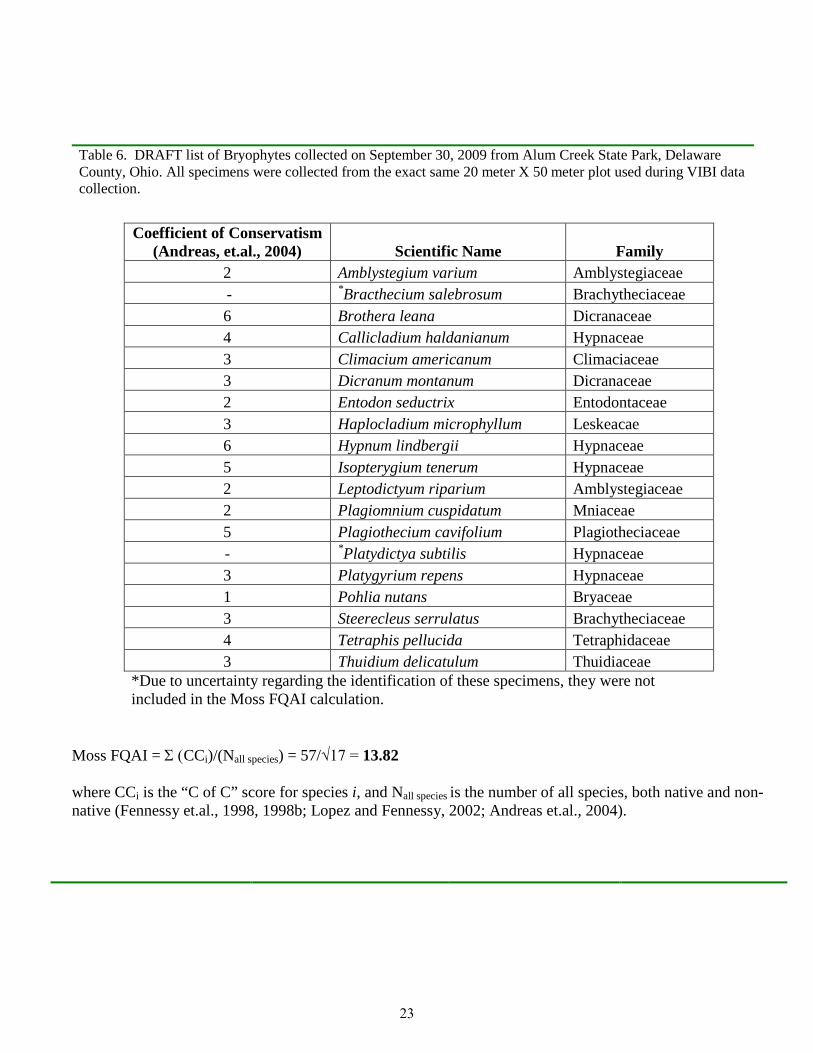
Table 6. DRAFT list of Bryophytes collected on September 30, 2009 from Alum Creek State Park, Delaware County, Ohio. All specimens were collected from the exact same 20 meter X 50 meter plot used during VIBI data collection.

Coefficient of Conservatism (Andreas, et.al., 2004) Scientific Name Family

2 Amblystegium varium Amblystegiaceae - *Bracthecium salebrosum Brachytheciaceae 6 Brothera leana Dicranaceae 4 Callicladium haldanianum Hypnaceae 3 Climacium americanum Climaciaceae 3 Dicranum montanum Dicranaceae 2 Entodon seductrix Entodontaceae 3 Haplocladium microphyllum Leskeacae 6 Hypnum lindbergii Hypnaceae 5 Isopterygium tenerum Hypnaceae 2 Leptodictyum riparium Amblystegiaceae 2 Plagiomnium cuspidatum Mniaceae 5 Plagiothecium cavifolium Plagiotheciaceae - *Platydictya subtilis Hypnaceae 3 Platygyrium repens Hypnaceae 1 Pohlia nutans Bryaceae 3 Steerecleus serrulatus Brachytheciaceae 4 Tetraphis pellucida Tetraphidaceae 3 Thuidium delicatulum Thuidiaceae

*Due to uncertainty regarding the identification of these specimens, they were not included in the Moss FQAI calculation.

Moss FQAI = Σ (CCi)/(Nall species) = 57/√17 = 13.82 where CCi is the “C of C” score for species i, and Nall species is the number of all species, both native and non-native (Fennessy et.al., 1998, 1998b; Lopez and Fennessy, 2002; Andreas et.al., 2004).

23

Figure 1. Ohio Statewide Imagery Program (OSIP) true color orthophotography for Lawrence Woods State Nature Preserve, Hardin County, Ohio.

24

Figure 2. 2006 Ohio Statewide Imagery Program (OSIP) color infrared orthophotography for Lawrence Woods State Nature Preserve, Hardin County, Ohio.

25

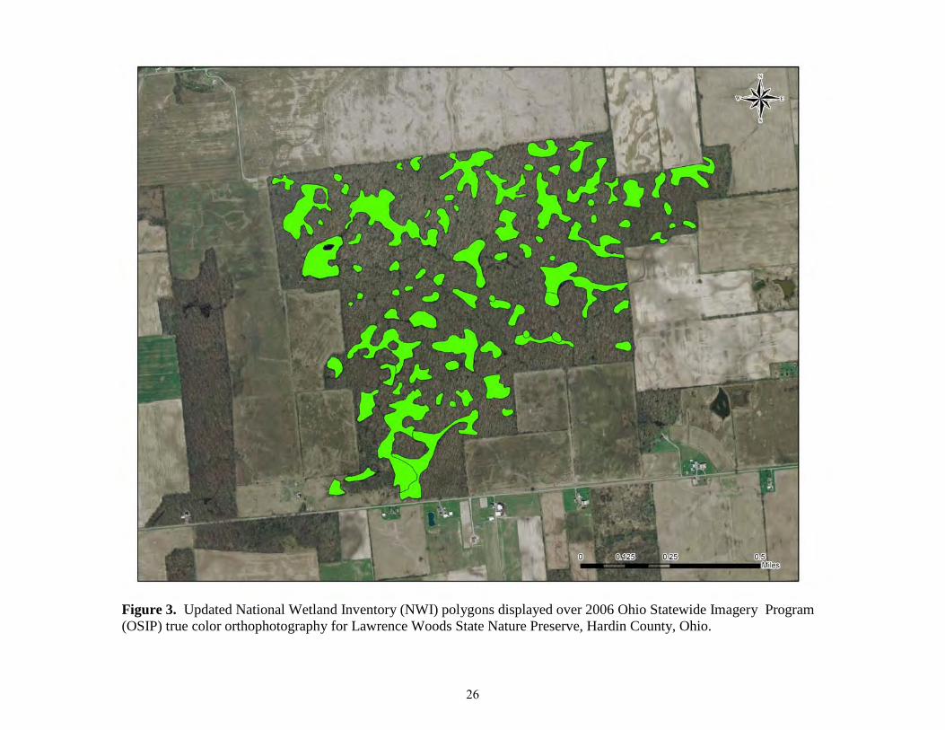
Figure 3. Updated National Wetland Inventory (NWI) polygons displayed over 2006 Ohio Statewide Imagery Program (OSIP) true color orthophotography for Lawrence Woods State Nature Preserve, Hardin County, Ohio.

26

Figure 4. Shrub swamp in Kokosing Wildlife Area depicting inner (0 to 100 meters) and outer (100 to 350) buffer zones surrounding the wetland, displayed over 2006 Ohio Statewide Imagery Program (OSIP) true color orthophotography.

27

Figure 5. Locations of 2009 monitoring sites to field verify Level 1 GIS model to assess the ecological integrity of areas surrounding updated NWI wetlands in Ohio.

28

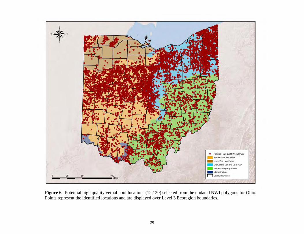
Figure 6. Potential high quality vernal pool locations (12,120) selected from the updated NWI polygons for Ohio. Points represent the identified locations and are displayed over Level 3 Ecoregion boundaries.

29

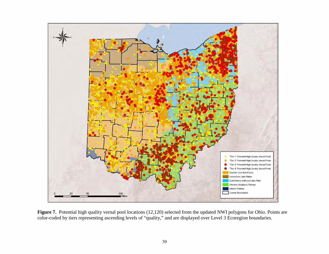
Figure 7. Potential high quality vernal pool locations (12,120) selected from the updated NWI polygons for Ohio. Points are color-coded by tiers representing ascending levels of “quality,” and are displayed over Level 3 Ecoregion boundaries.

30

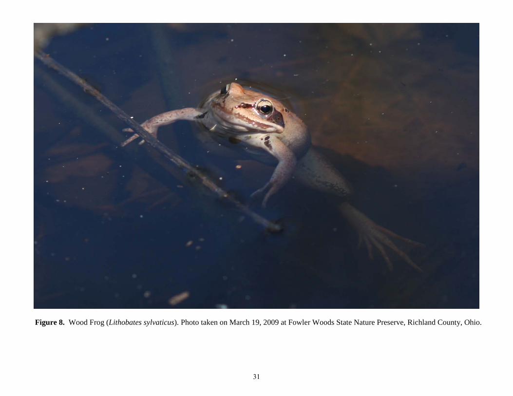
Figure 8. Wood Frog (Lithobates sylvaticus). Photo taken on March 19, 2009 at Fowler Woods State Nature Preserve, Richland County, Ohio.

31

Figure 9. Spotted Salamander (Ambystoma maculatum) egg masses. Photo taken on April 9, 2009 at Alum Creek State Park beach vernal pool, Delaware County, Ohio.

32

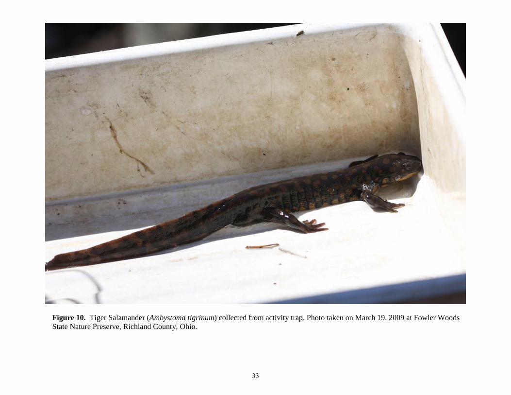
Figure 10. Tiger Salamander (Ambystoma tigrinum) collected from activity trap. Photo taken on March 19, 2009 at Fowler Woods State Nature Preserve, Richland County, Ohio.

33

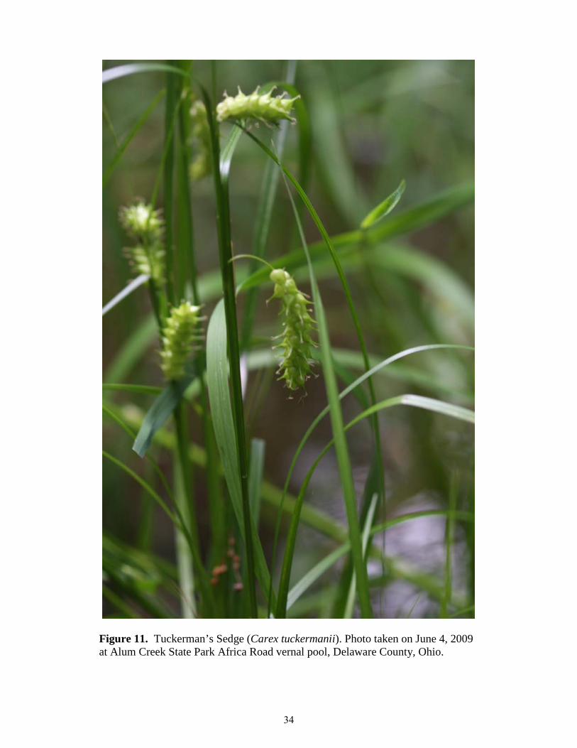
Figure 11. Tuckerman’s Sedge (Carex tuckermanii). Photo taken on June 4, 2009 at Alum Creek State Park Africa Road vernal pool, Delaware County, Ohio.

34

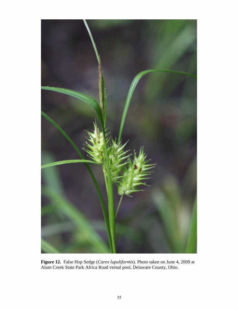
Figure 12. False Hop Sedge (Carex lupuliformis). Photo taken on June 4, 2009 at Alum Creek State Park Africa Road vernal pool, Delaware County, Ohio.

35

Figure 13. Vernal pool restoration locations (3,034) for Ohio. All potential high quality vernal pools were buffered 500 meters. Only buffer areas consisting of >10% historic wetland and >10% agriculture land use (row crop or pasture) have been included.

36

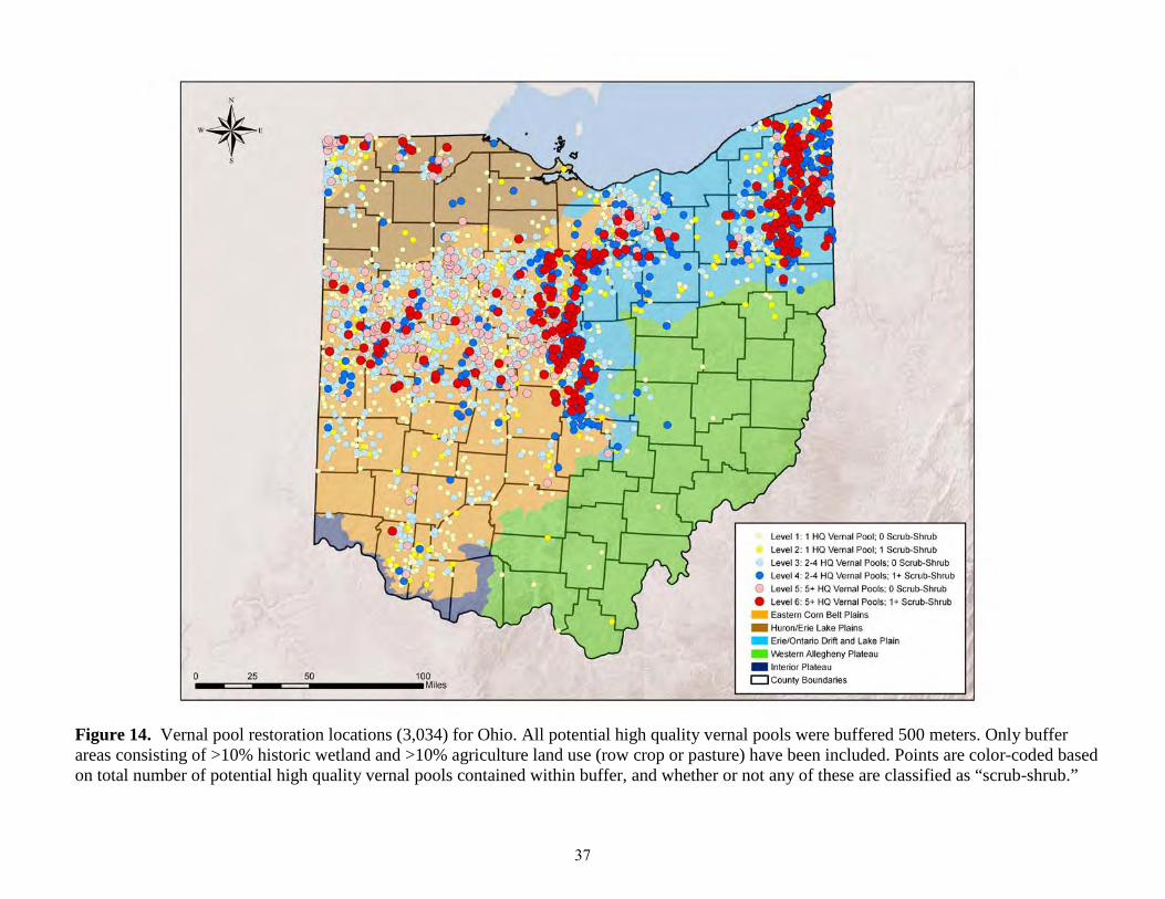
Figure 14. Vernal pool restoration locations (3,034) for Ohio. All potential high quality vernal pools were buffered 500 meters. Only buffer areas consisting of >10% historic wetland and >10% agriculture land use (row crop or pasture) have been included. Points are color-coded based on total number of potential high quality vernal pools contained within buffer, and whether or not any of these are classified as “scrub-shrub.”

37

Figure 15. Example potential vernal pool restoration site for area surrounding Morris Woods State Nature Preserve, Licking County, Ohio. Displayed over 2006 Ohio Statewide Imagery Program (OSIP) true color orthophotography.

38