Embed Size (px)
Citation preview
Assessment of Groundwater Input and Water Quality Changes Impacting Natural Vegetation in the Loxahatchee River and Floodplain Ecosystem, Florida By William H. Orem, Peter W. Swarzenski, Benjamin F. McPherson, Marion Hedgepath,
Harry E. Lerch, Christopher Reich, Arturo E. Torres, Margo D. Corum, and Richard E. Roberts
Open-File Report 2007-1304 U.S. Department of the Interior U.S. Geological Survey
1
U.S. Department of the Interior DIRK KEMPTHORNE, Secretary
U.S. Geological Survey Mark D. Myers, Director
U.S. Geological Survey, Reston, Virginia 20192
For product and ordering information: World Wide Web: http://www.usgs.gov/pubprod Telephone: 1-888-ASK-USGS For more information on the USGS—the Federal source for science about the Earth, its natural and living resources, natural hazards, and the environment: World Wide Web: http://www.usgs.gov Telephone: 1-888-ASK-USGS Suggested citation: Orem, W., and others, 2007, Assessment of Groundwater Input and Water Quality Changes Impacting Natural Vegetation in the Loxahatchee River and Floodplain Ecosystem, Florida: U.S. Geological Survey Open-File Report 2007-1304. Any use of trade, product, or firm names is for descriptive purposes only and does not imply endorsement by the U.S. Government. Although this report is in the public domain, permission must be secured from the individual copyright owners to reproduce any copyrighted material contained within this report.
2
Table of Contents
Page List of Figures ..................................................................................................................................... 5
List of Tables...................................................................................................................................... 7
Conversion Factors ............................................................................................................................. 8
Abbreviations...................................................................................................................................... 9
Summary............................................................................................................................................. 10
I. Introduction ..................................................................................................................................... 12
I.A. Background.......................................................................................................................... 12
I.B. Objectives............................................................................................................................. 17
II. Retrospective.................................................................................................................................. 19
II.A. General................................................................................................................................ 19
II.B. Influence of Saltwater Intrusion on Freshwater Vegetation............................................... 19
II.C. Long-Term Patterns in Groundwater Levels and Rainfall................................................. 20
II.D. Long-term Patterns in Floodplain Vegetation.................................................................... 26
III. Study Area and Sampling............................................................................................................. 26
III.A. General Description........................................................................................................... 26
III.B. Loxahatchee River and Estuarine Sites............................................................................. 28
III.C. Loxahatchee River Floodplain Sites.................................................................................. 30
IV. Methods........................................................................................................................................ 41
IV.A. Groundwater Flux Measurements..................................................................................... 41
IV.B. Groundwater Flux Calculations........................................................................................ 42
IV.C. Analytical Methods for Chemical Species........................................................................ 43
IV.C.1. River and estuarine water column samples............................................................ 43
IV.C.2. Floodplain surface and pore water samples........................................................... 43
IV.C.3. Floodplain sediment samples................................................................................. 44
IV.D. Vegetation Analysis.................................................................................................. 46
V. Results............................................................................................................................................ 50
V.A. Loxahatchee River Water Column Chemical Measurements............................................ 50
V.A.1. General.................................................................................................................... 50
V.A.2. Trace elements and DOC......................................................................................... 54
V.A.3. Surface water Radium and Radon isotopes............................................................. 54
V.B. Loxahatchee River Floodplain Water Quality Measurements........................................... 59
V.B.1. General..................................................................................................................... 59
3
V.B.2. pH, alkalinity, and redox......................................................................................... 59
V.B.3. Conductivity, salinity, and total dissolved solids.................................................... 60
V.B.4. Chloride, fluoride, and bromide............................................................................... 62
V.B.5. Sulfate and sulfide....................................................................................................63
V.B.6. Nitrate, ammonium, and phosphate......................................................................... 66
V.B.7. Sodium, potassium, magnesium, and calcium......................................................... 68
V.C. Loxahatchee River Floodplain Sediment Chemistry.......................................................... 70
V.D. Floodplain Vegetation Communities.................................................................................. 71
VI. Discussion..................................................................................................................................... 79
VI.A. Loxahatchee River Geochemistry..................................................................................... 79
VI.A.1. General................................................................................................................... 79
VI.A.2. Biogeochemical estuarine trace element transport................................................. 79
VI.B. Groundwater Flux in Loxahatchee River.......................................................................... 84
VI.B.1. Ra-derived estuarine water mass ages.................................................................... 82
VI.B.2. Ra-derived submarine groundwater discharge models.......................................... 85
VI.B.3. Groundwater recharge estimates............................................................................ 87
VI.B.4. Electromagnetic seepage meter measurements...................................................... 88
VI.B.5. Surface water Rn-222 activities............................................................................. 88
VI.B.6. Subsurface streaming resistivity profiling measurements...................................... 89
VI.B.7. Groundwater-derived nutrient fluxes..................................................................... 89
VI.C. Water Chemistry – Loxahatchee River Floodplain........................................................... 92
VI.D. Sediment Geochemistry – Floodplain............................................................................... 94
VI.E. Water Quality and Vegetation Change in Floodplain....................................................... 94
VII. Conclusions................................................................................................................................. 97
VII.A. Groundwater and Chemical Flux..................................................................................... 97
VII.B. Floodplain Water Quality and Vegetation Change.......................................................... 97
Acknowledgments............................................................................................................................... 99
References Cited................................................................................................................................. 99
Appendix A – Loxahatchee River Floodplain Water Chemistry Tables
Appendix B - Loxahatchee River Floodplain Water Chemistry Figures
Appendix C – Loxahatchee River Floodplain Soil/Sediment Tables
Appendix D - Loxahatchee River Floodplain Soil/Sediment Chemistry Figures
Appendix E - Loxahatchee River Floodplain Forest Types
4
List of Figures in Text
Fig. 1. Map showing the location of the Loxahatchee River in south Florida (top), and satellite
image of the Loxahatchee River, its tributaries, and the surrounding watershed (bottom).
Images modified from Google Earth............................................................... ........................ 13
Fig. 2. Canoeing the North West Fork of the Loxahatchee River at Jonathan Dickinson
State Park............................................................................................................................. 14
Fig. 3. Map of the Loxahatchee River watershed, showing major canals and drainage features,
the location of wells (M_1234, M_140, Pb_565, Pb_689, Pb_1642, and Pb_ 1662)
installed by the U.S. Geological Survey, and approximate locations of maps in Figures
18 and 19.................................................................................................................................. 15
Fig. 4. Dead cypress tree along the Northwest Branch/Fork of the Loxahatchee River..................... 16
Fig. 5. Decline in the groundwater level in Loxahatchee River Well M-140, 1950-1990................. 21
Fig. 6. Decline in the groundwater level in Loxahatchee River well Pb-689, 1993-2003.................. 22
Fig. 7. Long-term rainfall patterns in southeastern coastal Florida.................................................... 23
Fig. 8. Deviations in annual rainfall for period of record, southeastern coast of Florida................... 24
Fig. 9. Deviations in annual rainfall for the period 1950-2003, southeastern coast of Florida.......... 25
Fig. 10. Mean daily streamflow (m3 sec-1) and precipitation (cm) for the Loxahatchee River
estuary. Individual sampling intervals are denoted by the vertical grey (Ra, elements)
and black (Rn) bars............................................................................................................. 28
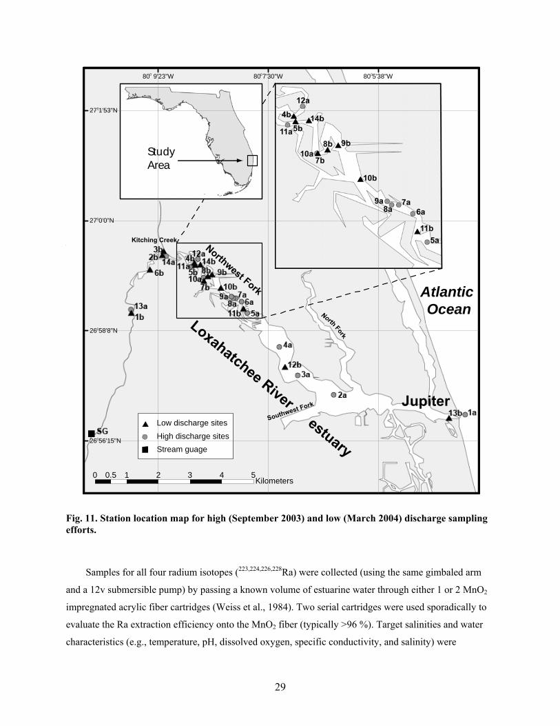
Fig. 11. Station location map for high (September 2003) and low (March 2004) discharge
sampling efforts................................................................................................................... 29
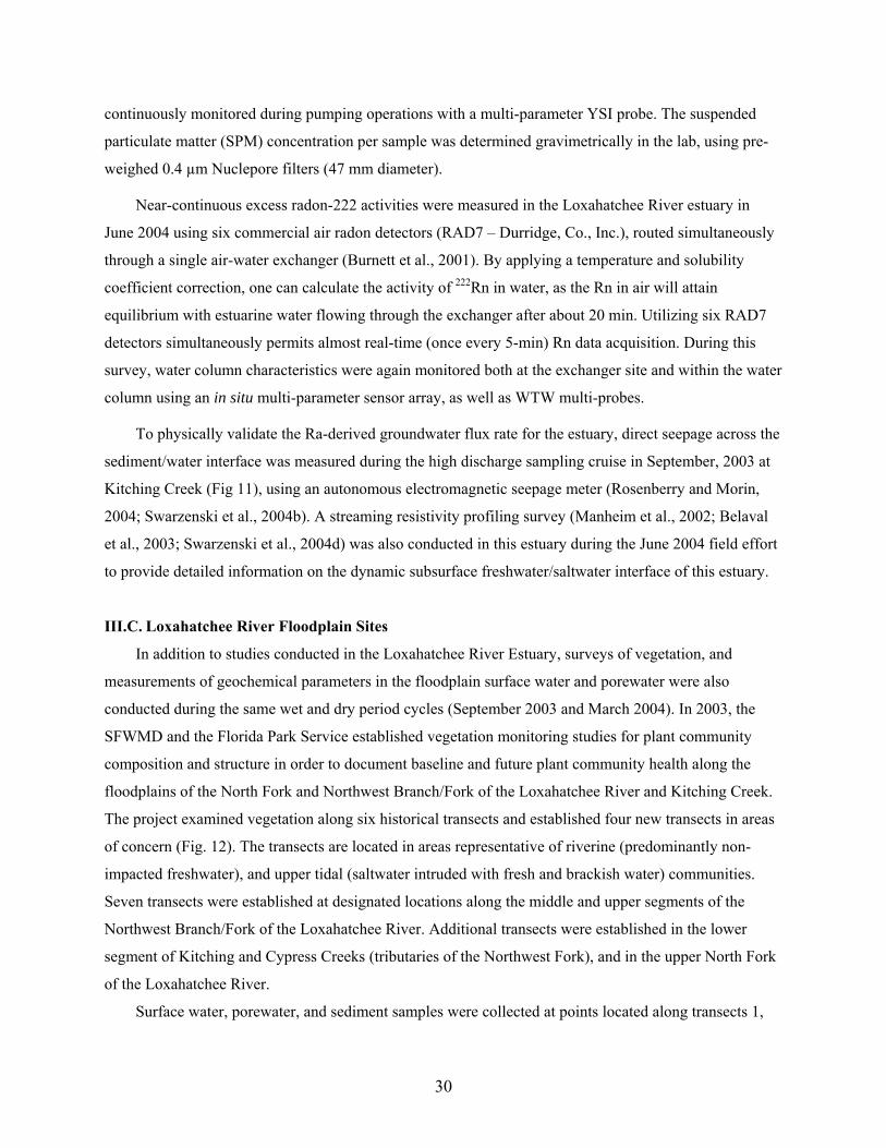
Fig. 12. Location of the 10 vegetative transects in the Loxahatchee River Floodplain...................... 31
Fig. 13. Map along Transect 1 in the Loxahatchee River floodplain, showing sampling locations
for surface water, pore water, and sediments, and the locations of wells sampled for
groundwater......................................................................................................................... 32
Fig. 14. Map along Transect 3 in the Loxahatchee River floodplain, showing sampling locations
for surface water, pore water, and sediments, and the locations of wells sampled for
groundwater......................................................................................................................... 33
Fig. 15. Map along Transect 6 in the Loxahatchee River floodplain, showing sampling locations
for surface water, pore water, and sediments, and the locations of wells sampled for
groundwater......................................................................................................................... 34
Fig. 16. Map along Transect 7 in the Loxahatchee River floodplain, showing sampling locations
for surface water, pore water, and sediments, and the locations of wells sampled for
groundwater......................................................................................................................... 35
5
Fig. 17. Map along Transect 9 in the Loxahatchee River floodplain, showing sampling locations
for surface water, pore water, and sediments, and the locations of wells sampled for
groundwater......................................................................................................................... 36
Fig. 18. Reaches of the Northwest Fork of the Loxahatchee River between river miles 4.5
and 13.................................................................................................................................. 48
Fig. 19. Upper riverine reach of the Northwest Fork of the Loxahatchee between I-95 and the
G-92 structure.............................................................................................................. ....... 49
Fig. 20. Salinity versus suspended particulate material (SPM), (a), and Dissolved Organic
Carbon (DOC), (b), for the two sampling periods.............................................................. 52
Fig. 21. Plots of salinity versus dissolved 224Ra (a) and 223Ra (b) for the two sampling periods....... 56
Fig. 22. Plots of salinity versus dissolved 228Ra (a) and 226Ra (b) for the two sampling periods....... 57
Fig. 23. Dissolved 222Rn activities (dpm L-1) in the Loxahatchee River estuary................................ 58
Fig. 24. Plots of concentrations of sodium (mg/L) versus chloride (mg/L) for pore water and
surface water from the floodplain of the Loxahatchee River during the wet season (A)
and the dry season (B)......................................................................................................... 69
Fig. 25. Plots of concentrations of calcium (mg/L) versus chloride (mg/L) for pore water and
surface water from the floodplain of the Loxahatchee River during the wet season (A)
and the dry season (B)......................................................................................................... 70
Fig. 26. Canopy species along Transect 1 in the Loxahatchee River floodplain................................ 73
Fig. 27. Canopy species along Transect 3 in the Loxahatchee River floodplain ............................... 74
Fig. 28. Canopy species along Transect 6 in the Loxahatchee River floodplain ............................... 75
Fig. 29. Canopy species along Transect 7 in the Loxahatchee River floodplain................................ 76
Fig. 30. Canopy species along Transect 9 in the Loxahatchee River floodplain................................ 78
Fig. 31. Salinity versus Cobalt (a) and Silicon (b), for the two sampling periods.............................. 80
Fig. 32. Salinity versus Manganese (a) and Iron (b), for the two sampling periods........................... 81
Fig. 33. Salinity versus Barium (a), and Strontium (b), for the two sampling periods....................... 82
Fig. 34. Salinity versus Uranium (a), and Vanadium (b), for the two sampling periods.................... 83
Fig. 35. A comparison of two modeled streaming resisitivity profiles, one proximal to Jupiter
Inlet in a saline environment (a), and one close to the confluence of Kitching Creek
and the Loxahatchee River (b)............................................................................................ 90
6
List of Tables in Text
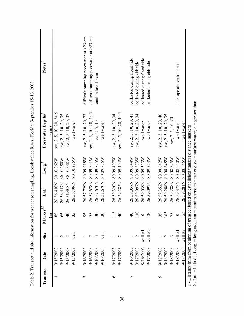
Table 1. Statistical analysis of groundwater levels in wells, Loxahatchee River, Florida..................22 Table 2. Transect and site information for Loxahatchee River wet season sampling,
September 15-18, 2003....................................................................................................... 38
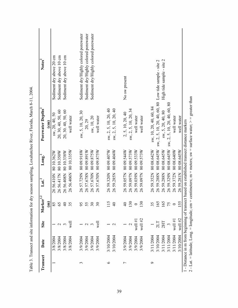
Table 3. Transect and site information for Loxahatchee River dry season sampling,
March 8-11, 2004................................................................................................................ 39
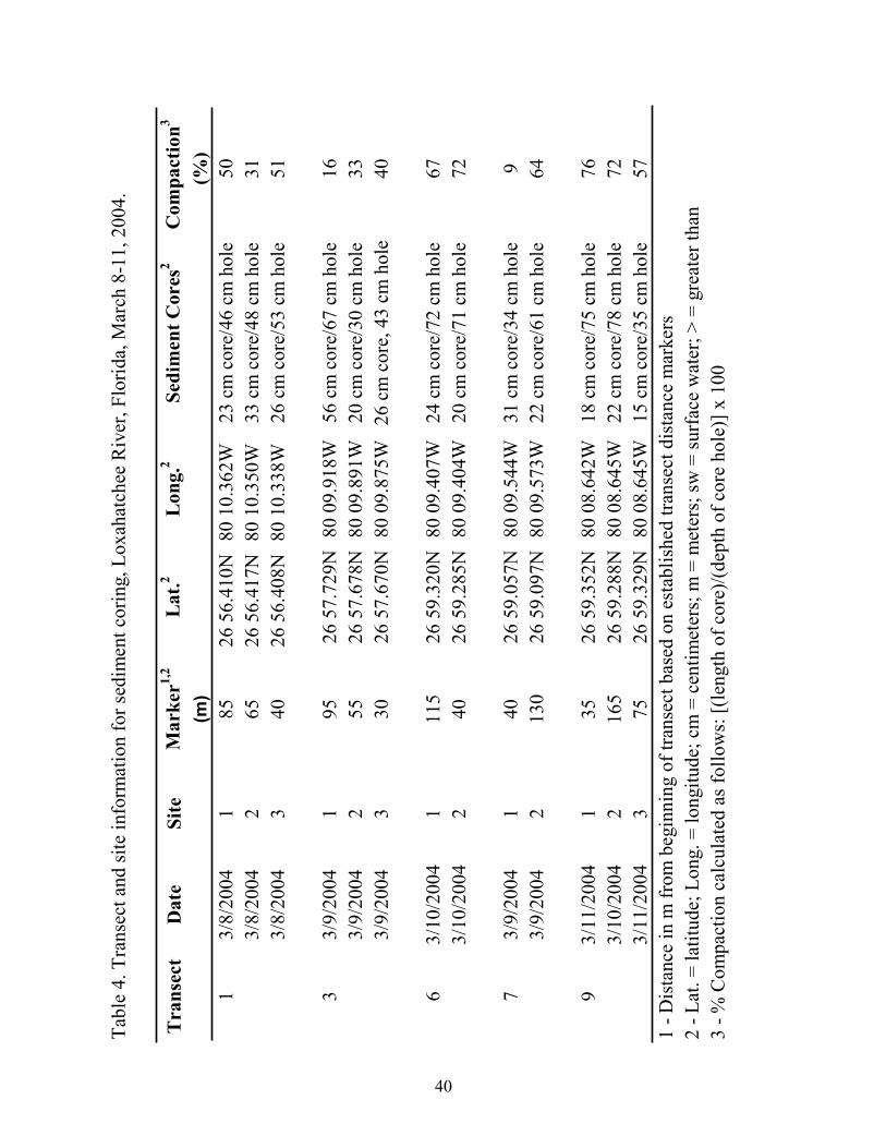
Table 4. Transect and site information for Loxahatchee River sediment coring,
March 8-11, 2004................................................................................................................ 40
Table 5. Methods used for sample collection and chemical analysis in the Loxahatchee River
Floodplain........................................................................................................................... 45
Table 6. Forest community types by reach for the Loxahatchee River and its major tributaries....... 50
Table 7. Chemical measurements of surface water in the Loxahatchee River in a transect from
seaward of Jupiter Inlet to the farthest reaches of the Northwest Fork............................... 51
Table 8. Dissolved organic carbon (DOC) and select trace element concentrations per river
discharge (season)............................................................................................................... 53
Table 9. Dissolved 226,228,223,224Ra activities and salinity in shallow groundwater wells adjacent
to the Loxahatchee River estuary per river discharge (season)........................................... 54
Table 10. Dissolved 226,228,223,224Ra activities and salinity in the Loxahatchee River estuary, per
river discharge (season)....................................................................................................... 55
Table 11. South Florida Water Management District 2003 canopy plant and code list..................... 72
Table 12. Radium-derived, and electromagnetic (EM) seepage meter-derived groundwater
discharge rate estimates for the Loxahatchee River estuary, per river discharge
(season)................................................................................................................................ 87
Table 13. Radium-derived nutrient (NH4+, PO4
3-) fluxes to the Loxahatchee River estuary,
per river discharge (season)................................................................................................. 91
7
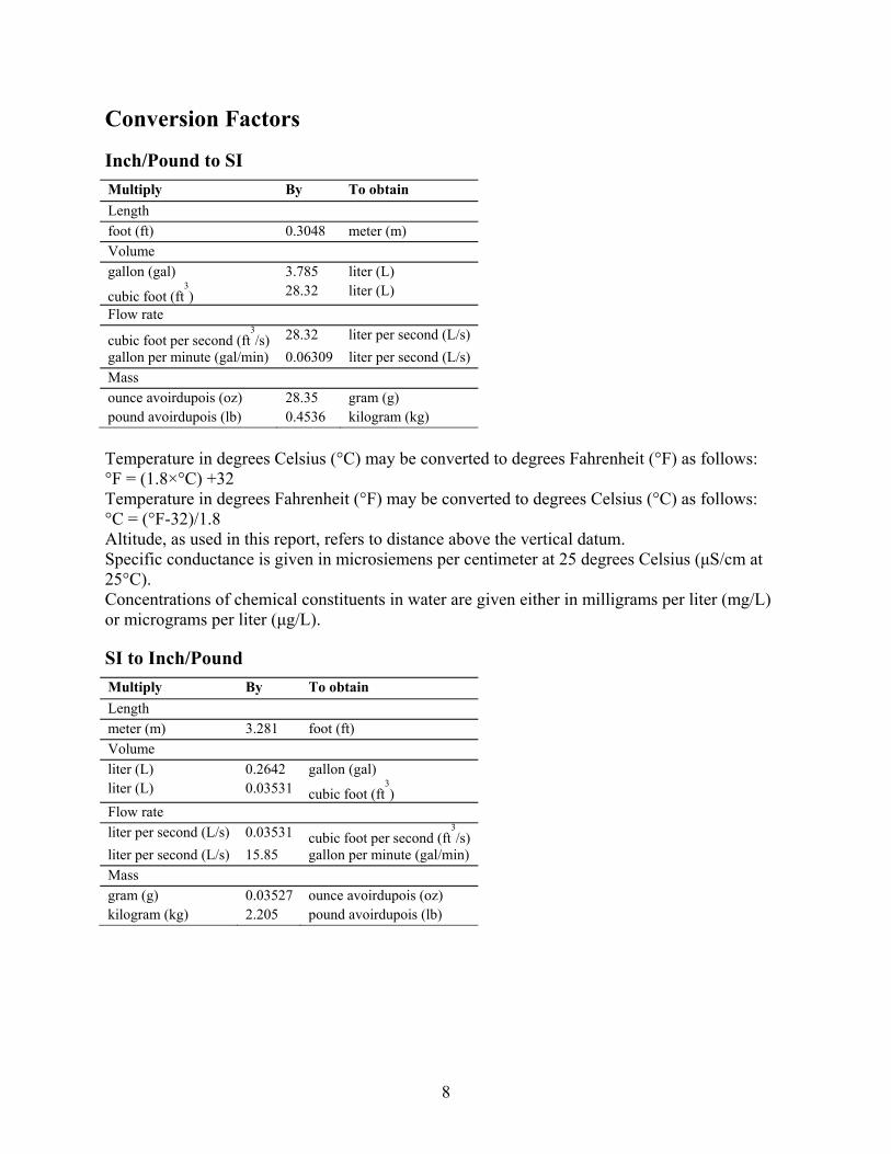
Conversion Factors
Inch/Pound to SI Multiply By To obtain Length foot (ft) 0.3048 meter (m) Volume gallon (gal) 3.785 liter (L)
cubic foot (ft3) 28.32 liter (L)
Flow rate
cubic foot per second (ft3/s) 28.32 liter per second (L/s)
gallon per minute (gal/min) 0.06309 liter per second (L/s) Mass ounce avoirdupois (oz) 28.35 gram (g) pound avoirdupois (lb) 0.4536 kilogram (kg) Temperature in degrees Celsius (°C) may be converted to degrees Fahrenheit (°F) as follows: °F = (1.8×°C) +32 Temperature in degrees Fahrenheit (°F) may be converted to degrees Celsius (°C) as follows: °C = (°F-32)/1.8 Altitude, as used in this report, refers to distance above the vertical datum. Specific conductance is given in microsiemens per centimeter at 25 degrees Celsius (μS/cm at 25°C). Concentrations of chemical constituents in water are given either in milligrams per liter (mg/L) or micrograms per liter (μg/L).
SI to Inch/Pound Multiply By To obtain Length meter (m) 3.281 foot (ft) Volume liter (L) 0.2642 gallon (gal) liter (L) 0.03531 cubic foot (ft
3)
Flow rate liter per second (L/s) 0.03531 cubic foot per second (ft
3/s)
liter per second (L/s) 15.85 gallon per minute (gal/min) Mass gram (g) 0.03527 ounce avoirdupois (oz) kilogram (kg) 2.205 pound avoirdupois (lb)
8
9
Abbreviations
‰ – parts per thousand (units for salinity), equivalent to gL-1
µmol – micromoles
µg - micrograms
d - day
dbh – diameter at breast height (measurement of tree dimension)
DIN – dissolved inorganic nitrogen
DOC – dissolved organic carbon
dpm – disintegrations per minute (for radioactive elements)
L - liter
LT – lower tidal
m – meters
m3 – cubic meteers
meq L-1 or meq/L – milliequivalents per liter
mg L-1 or mg/L – milligrams pre liter
MFLs – minimum flows and levels
NGVD – National Geodetic Vertical Datum
NPBC CERP – North Palm Beach County Comprehensive Everglades Restoration Plan
NW – northwest
OC – organic carbon
R – riverine
RBA – relative basal area (measurement of tree areal coverage)
RECOVER – Restoration Coordination and Verification (part of Comprehensive Everglades Restoration
Plan (CERP)
%RSD – percentage relative standard deviation
SFWMD – South Florida Water Management District
SGD – submarine groundwater discharge
SPM – suspended particulate material
TC – total carbon
TN – total nitrogen
TP – total phosphorus
TS – total sulfur
USGS – United States Geological Survey
UT – upper tidal
Assessment of Groundwater Input and Water Quality Changes Impacting Natural Vegetation in the Loxahatchee River and Floodplain Ecosystem, Florida
By William H. Orem1, Peter W. Swarzenski2, Benjamin F. McPherson3, Marion Hedgepath4,
Harry E. Lerch1, Christopher Reich2, Arturo E. Torres3, Margo D. Corum1, and Richard E.
Roberts5
1USGS, 956 National Center, Reston, VA 20192 2USGS, 600 4th St. S., St. Petersburg, FL 33701 3USGS, 10500 University Center Dr., Suite 215, Tampa, FL 33612 4South Florida Water Management District, 3301 Gun Club Road, West Palm Beach, FL 33406 5Florida Department of Environmental Protection, Florida Park Service, District 5, P.O. Box 1246,
Hobe Sound, FL 33455.
Summary The Loxahatchee River and Estuary are small, shallow, water bodies located in southeastern Florida.
Historically, the Northwest Branch (Fork) of the Loxahatchee River was primarily a freshwater system.
In 1947, the river inlet at Jupiter was dredged for navigation and has remained permanently open since
that time. Drainage patterns within the basin have also been altered significantly due to land
development, road construction (e.g., Florida Turnpike), and construction of the C-18 and other canals.
These anthropogenic activities along with sea level rise have resulted in significant adverse impacts on
the ecosystem over the last several decades, including increased saltwater encroachment and undesired
vegetation changes in the floodplain. The problem of saltwater intrusion and vegetation degradation in the
Loxahatchee River may be partly induced by diminished freshwater input, from both surface water and
ground water into the River system.
The overall objective of this project was to assess the seasonal surface water and groundwater
interaction and the influence of the biogeochemical characteristics of shallow groundwater and porewater
on vegetation health in the Loxahatchee floodplain. The hypothesis tested are: (1) groundwater influx
constitutes a significant component of the overall flow of water into the Loxahatchee River; (2) salinity
and other chemical constituents in shallow groundwater and porewater of the river floodplain may affect
the distribution and health of the floodplain vegetation.
10
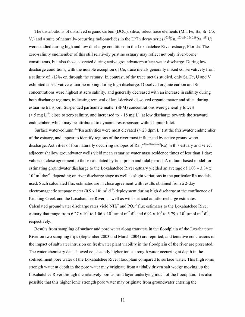
The distributions of dissolved organic carbon (DOC), silica, select trace elements (Mn, Fe, Ba, Sr, Co,
V,) and a suite of naturally-occurring radionuclides in the U/Th decay series (222Rn, 223,224,226,228Ra, 238U)
were studied during high and low discharge conditions in the Loxahatchee River estuary, Florida. The
zero-salinity endmember of this still relatively pristine estuary may reflect not only river-borne
constituents, but also those advected during active groundwater/surface-water discharge. During low
discharge conditions, with the notable exception of Co, trace metals generally mixed conservatively from
a salinity of ~12‰ on through the estuary. In contrast, of the trace metals studied, only Sr, Fe, U and V
exhibited conservative estuarine mixing during high discharge. Dissolved organic carbon and Si
concentrations were highest at zero salinity, and generally decreased with an increase in salinity during
both discharge regimes, indicating removal of land-derived dissolved organic matter and silica during
estuarine transport. Suspended particulate matter (SPM) concentrations were generally lowest
(< 5 mg L-1) close to zero salinity, and increased to ~ 18 mg L-1 at low discharge towards the seaward
endmember, which may be attributed to dynamic resuspension within Jupiter Inlet.
Surface water-column 222Rn activities were most elevated (> 28 dpm L-1) at the freshwater endmember
of the estuary, and appear to identify regions of the river most influenced by active groundwater
discharge. Activities of four naturally occurring isotopes of Ra (223,224,226,228Ra) in this estuary and select
adjacent shallow groundwater wells yield mean estuarine water mass residence times of less than 1 day;
values in close agreement to those calculated by tidal prism and tidal period. A radium-based model for
estimating groundwater discharge to the Loxahatchee River estuary yielded an average of 1.03 – 3.84 x
105 m3 day-1, depending on river discharge stage as well as slight variations in the particular Ra models
used. Such calculated flux estimates are in close agreement with results obtained from a 2-day
electromagnetic seepage meter (0.9 x 10⁵ m3 d-1) deployment during high discharge at the confluence of
Kitching Creek and the Loxahatchee River, as well as with surficial aquifer recharge estimates.
Calculated groundwater discharge rates yield NH4+ and PO4
-3 flux estimates to the Loxahatchee River
estuary that range from 6.27 x 101 to 1.06 x 10³ µmol m-2 d-1 and 6.92 x 101 to 3.79 x 10² µmol m-2 d-1,
respectively.
Results from sampling of surface and pore water along transects in the floodplain of the Loxahatchee
River on two sampling trips (September 2003 and March 2004) are reported, and tentative conclusions on
the impact of saltwater intrusion on freshwater plant viability in the floodplain of the river are presented.
The water chemistry data showed consistently higher ionic strength water occurring at depth in the
soil/sediment pore water of the Loxahatchee River floodplain compared to surface water. This high ionic
strength water at depth in the pore water may originate from a tidally driven salt wedge moving up the
Loxahatchee River through the relatively porous sand layer underlying much of the floodplain. It is also
possible that this higher ionic strength pore water may originate from groundwater entering the
11
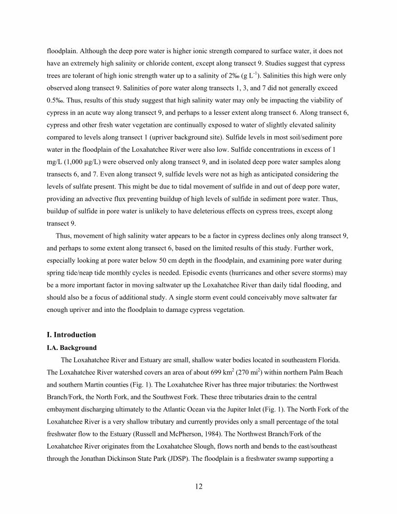
floodplain. Although the deep pore water is higher ionic strength compared to surface water, it does not
have an extremely high salinity or chloride content, except along transect 9. Studies suggest that cypress
trees are tolerant of high ionic strength water up to a salinity of 2‰ (g L-1). Salinities this high were only
observed along transect 9. Salinities of pore water along transects 1, 3, and 7 did not generally exceed
0.5‰. Thus, results of this study suggest that high salinity water may only be impacting the viability of
cypress in an acute way along transect 9, and perhaps to a lesser extent along transect 6. Along transect 6,
cypress and other fresh water vegetation are continually exposed to water of slightly elevated salinity
compared to levels along transect 1 (upriver background site). Sulfide levels in most soil/sediment pore
water in the floodplain of the Loxahatchee River were also low. Sulfide concentrations in excess of 1
mg/L (1,000 µg/L) were observed only along transect 9, and in isolated deep pore water samples along
transects 6, and 7. Even along transect 9, sulfide levels were not as high as anticipated considering the
levels of sulfate present. This might be due to tidal movement of sulfide in and out of deep pore water,
providing an advective flux preventing buildup of high levels of sulfide in sediment pore water. Thus,
buildup of sulfide in pore water is unlikely to have deleterious effects on cypress trees, except along
transect 9.
Thus, movement of high salinity water appears to be a factor in cypress declines only along transect 9,
and perhaps to some extent along transect 6, based on the limited results of this study. Further work,
especially looking at pore water below 50 cm depth in the floodplain, and examining pore water during
spring tide/neap tide monthly cycles is needed. Episodic events (hurricanes and other severe storms) may
be a more important factor in moving saltwater up the Loxahatchee River than daily tidal flooding, and
should also be a focus of additional study. A single storm event could conceivably move saltwater far
enough upriver and into the floodplain to damage cypress vegetation.
I. Introduction
I.A. Background
The Loxahatchee River and Estuary are small, shallow water bodies located in southeastern Florida.
The Loxahatchee River watershed covers an area of about 699 km2 (270 mi2) within northern Palm Beach
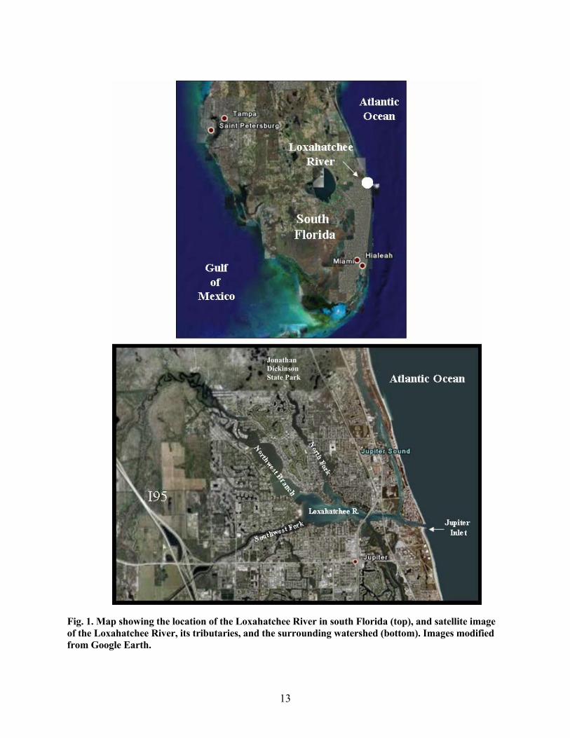
and southern Martin counties (Fig. 1). The Loxahatchee River has three major tributaries: the Northwest
Branch/Fork, the North Fork, and the Southwest Fork. These three tributaries drain to the central
embayment discharging ultimately to the Atlantic Ocean via the Jupiter Inlet (Fig. 1). The North Fork of the
Loxahatchee River is a very shallow tributary and currently provides only a small percentage of the total
freshwater flow to the Estuary (Russell and McPherson, 1984). The Northwest Branch/Fork of the
Loxahatchee River originates from the Loxahatchee Slough, flows north and bends to the east/southeast
through the Jonathan Dickinson State Park (JDSP). The floodplain is a freshwater swamp supporting a
12
Jonathan Dickinson State Park
Fig. 1. Map showing the location of the Loxahatchee River in south Florida (top), and satellite image of the Loxahatchee River, its tributaries, and the surrounding watershed (bottom). Images modified from Google Earth.
13
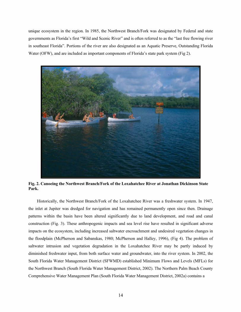
unique ecosystem in the region. In 1985, the Northwest Branch/Fork was designated by Federal and state
governments as Florida’s first “Wild and Scenic River” and is often referred to as the “last free flowing river
in southeast Florida”. Portions of the river are also designated as an Aquatic Preserve, Outstanding Florida
Water (OFW), and are included as important components of Florida’s state park system (Fig 2).
Fig. 2. Canoeing the Northwest Branch/Fork of the Loxahatchee River at Jonathan Dickinson State Park.
Historically, the Northwest Branch/Fork of the Loxahatchee River was a freshwater system. In 1947,
the inlet at Jupiter was dredged for navigation and has remained permanently open since then. Drainage
patterns within the basin have been altered significantly due to land development, and road and canal
construction (Fig. 3). These anthropogenic impacts and sea level rise have resulted in significant adverse
impacts on the ecosystem, including increased saltwater encroachment and undesired vegetation changes in
the floodplain (McPherson and Sabanskas, 1980; McPherson and Halley, 1996), (Fig 4). The problem of
saltwater intrusion and vegetation degradation in the Loxahatchee River may be partly induced by
diminished freshwater input, from both surface water and groundwater, into the river system. In 2002, the
South Florida Water Management District (SFWMD) established Minimum Flows and Levels (MFLs) for
the Northwest Branch (South Florida Water Management District, 2002). The Northern Palm Beach County
Comprehensive Water Management Plan (South Florida Water Management District, 2002a) contains a
14
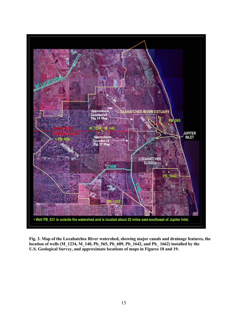
Fig. 3. Map of the Loxahatchee River watershed, showing major canals and drainage features, the location of wells (M_1234, M_140, Pb_565, Pb_689, Pb_1642, and Pb_ 1662) installed by the U.S. Geological Survey, and approximate locations of maps in Figures 18 and 19.
15
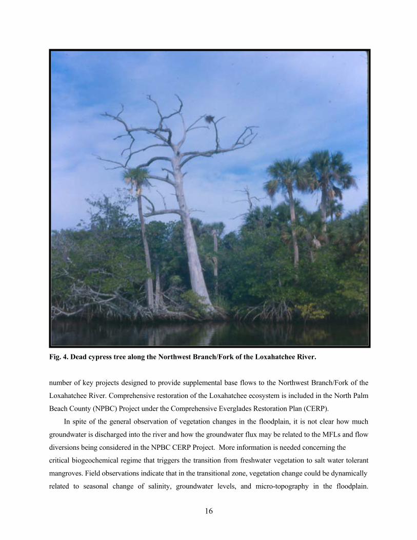
Fig. 4. Dead cypress tree along the Northwest Branch/Fork of the Loxahatchee River.
number of key projects designed to provide supplemental base flows to the Northwest Branch/Fork of the
Loxahatchee River. Comprehensive restoration of the Loxahatchee ecosystem is included in the North Palm
Beach County (NPBC) Project under the Comprehensive Everglades Restoration Plan (CERP).
In spite of the general observation of vegetation changes in the floodplain, it is not clear how much
groundwater is discharged into the river and how the groundwater flux may be related to the MFLs and flow
diversions being considered in the NPBC CERP Project. More information is needed concerning the
critical biogeochemical regime that triggers the transition from freshwater vegetation to salt water tolerant
mangroves. Field observations indicate that in the transitional zone, vegetation change could be dynamically
related to seasonal change of salinity, groundwater levels, and micro-topography in the floodplain.
16
Understanding the relationships among the surface water and groundwater interaction and its influence on
floodplain vegetation is critical to the future revision of the Loxahatchee MFLs and the NPBC CERP
Project. The project work reported here represents a cooperative agreement between the SFWMD and the
U.S. Geological Survey (USGS) to help address these issues.
I.B. Objectives
The overall objective of this project was to assess the seasonal surface water and groundwater
interaction and the influence of the biogeochemical characteristics of shallow groundwater and porewater
on vegetation health in the Loxahatchee River floodplain. The hypotheses being tested are: (1)
groundwater influx constitutes a significant component of the overall flow of water into the Loxahatchee
River; (2) salinity and other chemical constituents in shallow groundwater and porewater of the river
floodplain may affect the distribution and health of the floodplain vegetation.
We investigated the distributions of dissolved organic carbon (DOC), Si, select trace elements (Mn,
Fe, Ba, Sr, Co, V) and a suite of naturally occurring U/Th-series isotopes (222Rn, 223,224,226,228Ra, 238U)
during estuarine transport and mixing in the Loxahatchee River estuary. This subtropical estuary, located
just east of Lake Okeechobee, FL in a predominantly carbonate geologic environment (McPherson et al.,
1982; Wanless et al., 1984; Noel et al., 1995), may consequently have a strong groundwater contribution
to the surface-water budget (Russell and McPherson, 1984; Russell and Goodwin, 1987). Therefore, we
utilize naturally occurring isotopes of Ra and Rn as tracers of submarine groundwater flow in our
investigation of biogeochemical transport in the Loxahatchee River estuary (Cable et al., 1996, 1997;
Kelly and Moran, 1999; Krest et al., 1999, 2000; Swarzenski et al., 2001; Kelly and Moran, 2002; Burnett
and Dulaiova, 2003; Krest and Harvey, 2003; Charette and Buesseler, 2004; Purkl and Eisenhauer, 2004).
Estuaries are well-known biogeochemical reactors (Sholkovitz, 1976, 1977; Boyle et al., 1977;
Sholkovitz et al., 1978; Shiller and Boyle, 1991; Millward and Turner, 1994; Swarzenski et al., 1995)
wherein terrigenous material, carried downstream by rivers, eventually is mixed into seawater (Turekian,
1977). The reactions and processes that occur during estuarine mixing are similarly well-characterized
(Mackin and Aller, 1984; Yan et al., 1990; Chiffoleau et al., 1994; Robert et al., 2004; Turner et al.,
2004), and reflect an integration of diverse biogeochemical controls across land-sea margins (Martino et
al., 2004). For example, many estuarine systems are variably contaminated by anthropogenic inputs that
may influence estuarine transport and mixing (Shank et al., 2004). In addition, the ubiquitous nature of
groundwater discharge along many coastlines may directly affect estuarine water and geochemical
budgets alike (Bokuniewicz, 1980; Johannes, 1980; Oberdorfer et al., 1990; Valiela et al., 1990; Moore,
1996, 1997, 1999; Corbett et al., 1999; Li et al., 1999; Charette et al., 2001; Swarzenski et al., 2001;
Burnett et al., 2001, 2002, 2003; Slomp and Cappellen, 2004; Swarzenski et al., 2004a). To better
17
understand biogeochemical transport in the Loxahatchee River estuary, we have employed a suite of
natural tracers that can provide information on traditional biogeochemical scavenging reactions initiated
by an increase in salinity, as well as on the role of groundwater/surface water exchange or groundwater
discharge in impacting or defining such estuarine biogeochemical transport.
The USGS has in-house radiometric techniques (Radium [Ra] and Radon [Rn] isotopes) and
analytical expertise to examine freshwater-saltwater interactions and geochemical regimes of groundwater
and porewater in the wetland ecosystems of South Florida (e.g., Orem et al., 1997; Swarzenski, 2001). In
addition, the SFWMD has ongoing efforts in model development and groundwater and vegetation
monitoring in the floodplain of the Northwest Branch/Fork of the Loxahatchee River to address project
objectives.
This study addresses the following specific objectives:
• To evaluate long-term patterns in groundwater levels and rainfall in the Loxahatchee River
watershed from a literature survey.
• To characterize the Ra-Rn isotopic signature of surface water and groundwater within the
Loxahatchee River and Estuary; and to use these signatures and other indicators to estimate a wet
season and dry season groundwater input into the river system
• To measure salinity and other selected water-quality constituents in the sediment, porewater and
shallow groundwater of the river and floodplain during a wet and a dry season, and to relate
these measurements to the distribution and health of wetland vegetation in the Northwest
Branch/Fork of the Loxahatchee River.
To achieve these objectives, water samples from selected wells and from the surrounding surface
waters were collected and analyzed for Ra and Rn isotopes. Samples of porewater and sediment were
collected along selected SFWMD vegetation transects in the Loxahatchee River system (including
saltwater-impacted and pristine freshwater areas) for chemical analysis of selected parameters.
Parameters measured included: salinity, major ions (indicators of saltwater intrusion), sulfur species
(sulfate and sulfide), nutrients (nitrate, ammonium, phosphate), pH, alkalinity, redox conditions, and
dissolved oxygen. Comparing these geochemical parameters in both pristine freshwater and saltwater-
impacted sites provides a first step in determining the causes of the observed vegetation community
changes. An evaluation of the results in the context of existing studies of the sensitivity of freshwater
vegetation to changes in water quality provides a basis for determining the most important water quality
constituents. The information from our study will help support and contribute to several SFWMD efforts,
including flow and salinity modeling in the Estuary and floodplain, vegetation and soil studies in the
floodplain, the NPBC CERP Project and RECOVER, as well as the MFLs update and rule development for
the Loxahatchee River.
18
II. Retrospective
II.A. General
The SFWMD (2002) conducted a comprehensive environmental study of the Loxahatchee River.
The study included a literature review of environmental reports on the river over the past three decades.
The review includes studies related to saltwater intrusion and the effects of salinity on freshwater
vegetation, including cypress, and cites 76 references. The SFWMD study also includes an analysis of
historical vegetation distribution and changes in vegetation distribution along the Northwest Branch/Fork
of the Loxahatchee River. Other parts of the study document vegetation surveys, freshwater inflows, and
salinity along the Northwest Branch/Fork of the river. The study also presents preliminary results of
hydrodynamic and salinity models of the river and its estuary.
Studies of groundwater and its effects on wetland ecology in the vicinity of the Loxahatchee River
are much less common than those of surface water and its effects on wetland ecology. Shaw and Huffman
(2000) reported on the hydrology of isolated wetlands, including a wetland in Jonathan Dickenson State
Park, and how wetlands are affected by water table drawdown. Earth Tech, Inc (2000) conducted a study
of ground water in the Kitchen Creek basin just north of the Northwest Branch/Fork of the Loxahatchee
River .
II.B. Influence of Saltwater Intrusion on Freshwater Vegetation
Saltwater intrusion has been shown to adversely impact freshwater plants. High levels of salt may
cause problems of osmoregulation in plants not adapted to live in high ionic strength waters. In coastal
Louisiana, intrusion of seawater into freshwater and brackish marshes has resulted in significant
degradation of these wetlands through the mortality of macrophytes and other rooted plants (Flynn et al.,
1995; Howard et al., 2000; Hester et al., 2001; Holm et al., 2001).
In addition to the effects of salt, sulfate is also present in high concentrations in seawater (~2.7 g/L
of seawater). While sulfate itself is not harmful to macrophytes and other aquatic plants (except as it
contributes to the general salt issue), sulfate entering a wetland stimulates microbial sulfate reduction and
the production of toxic hydrogen sulfide. Sulfate reduction occurs in reducing environments, such as
wetland sediments (Bates et al., 2001). It is typically a minor metabolic process in freshwater sediments,
where methanogenesis dominates. Intrusion of saltwater or other major sources of sulfate, however, can
stimulate sulfate reduction and the production of hydrogen sulfide. Hydrogen sulfide can act as a toxin to
rooted aquatic vegetation in three ways: (1) reducing redox conditions in sediments and retarding
transport of oxygen to plant roots, (2) reacting with metals to form insoluble metal sulfides and depriving
plants of needed metal micronutrients, and (3) inhibiting uptake of nutrients from the sediments (Portnoy
and Giblin, 1997; Howard et al., 1999; Flynn et al., 1999; Lamers et al., 2002). In coastal Louisiana,
19
production of toxic hydrogen sulfide from saltwater intrusion may be the major factor in the loss of
freshwater and brackish marsh vegetation (Flynn et al., 1999). Sulfate is also entering the northern
Everglades at concentrations 50-100 times background (Orem et al., 1997, 1998, 2000; Orem, 2004;
Gilmour et al. 2007), and may be partly responsible for the changes in macrophyte distributions (cattail
replacing sawgrass) and tree island loss. In the case of the northern Everglades, however, the excess
sulfate originates from agricultural sources in the Everglades Agricultural Area rather than from seawater
intrusion (Orem et al., 2000; Bates et al., 2001). Regardless of the source, the sulfate entering the northern
Everglades has stimulated sulfate reduction, and drastically reduced redox conditions in the most heavily
affected areas (Orem et al., 1998; Gilmour et al., 2007). In the northern Everglades, excess nutrient inputs
from agricultural runoff have also been implicated in observed changes in macrophytes in the ecosystem,
with cattails replacing sawgrass (Vaithiyanathan and Richardson, 1999). Excess nutrient inputs can also
have dramatic effects on algal communities, with green algae replacing periphyton in eutrophied areas of
the Everglades (Noe et al., 2002).
II.C. Long-Term Patterns in Groundwater Levels and Rainfall
Long-term groundwater level measurements for shallow wells in the Loxahatchee River watershed
(Fig. 3) extend back to at least 1950. The shallow groundwater well with one of the longest records, M-
140, begins in 1950 and ends in 1990. Over this 40 year span, the groundwater level declined over 0.6 m
(2 ft), or about 0.02 m/yr (0.06 ft/year), (Fig. 5). During the 1990’s and early 2000’s, other wells were
installed and monitored. Statistical analyses generally indicate decreasing water level trends through this
period (Table 1). For example, well M-1234, located a few miles from M-140, declined 0.007 m/yr (0.024
ft/yr) between 1989 and 2004. Well Pb-689 declined 0.021 m/yr or 0.069 ft/yr (linear regression) from
1993-2003 (Fig. 6). The reason for the recent decline in groundwater levels is uncertain, and may have
multiple causes, including changes in long-term rainfall (Figs. 7 and 8), or various water management
activities in the watershed. However, the overall decline in groundwater level from 1950 to the present
spans years of heavy and light rainfall (Fig. 9). Thus the groundwater decline probably reflects drainage
alterations in the watershed, rather than patterns of rainfall. Drought conditions prevailed in 1989-1990
(Fig. 9), and groundwater levels were low as a result. Groundwater levels rebounded in the early 1990’s
as rainfall increased. Lower rainfall in the late 1990’s and early 2000’s may have contributed to overall
downward trends. Water management, including diversions, pumping, or impoundment, will normally
affect groundwater levels, and these effects will vary with location in the watershed. The predominant
trend, however, is downward, and the reduced groundwater head must have resulted in reduced
groundwater inflow to the river. Undoubtedly, many of the anthropogenic and natural effects on
groundwater levels in the Loxahatchee River watershed preceded recent groundwater monitoring.
20
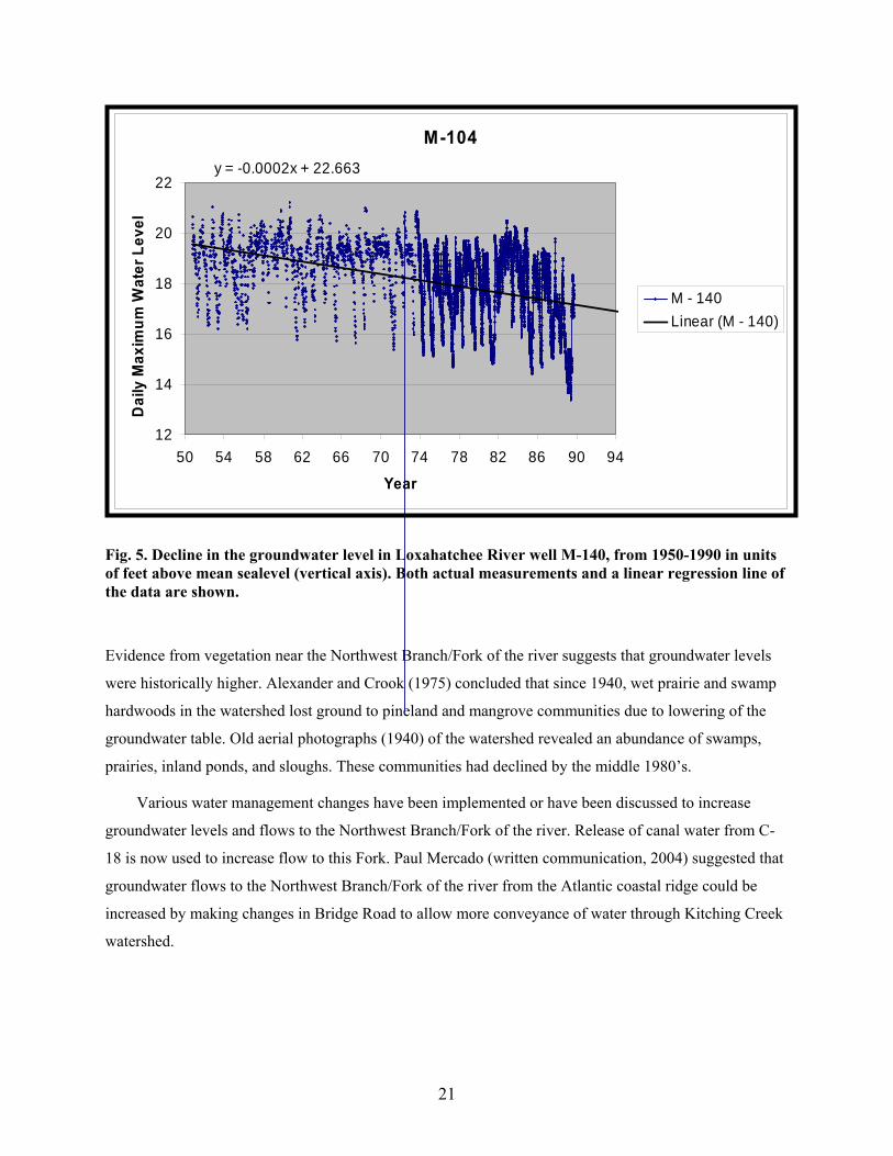
Fig. 5. Decline in the groundwater level in Loxahatchee River well M-140, from 1950-1990 in units of feet above mean sealevel (vertical axis). Both actual measurements and a linear regression line of the data are shown.
Evidence from vegetation near the Northwest Branch/Fork of the river suggests that groundwater levels
were historically higher. Alexander and Crook (1975) concluded that since 1940, wet prairie and swamp
hardwoods in the watershed lost ground to pineland and mangrove communities due to lowering of the
groundwater table. Old aerial photographs (1940) of the watershed revealed an abundance of swamps,
prairies, inland ponds, and sloughs. These communities had declined by the middle 1980’s.
M-104y = -0.0002x + 22.663
12
14
16
18
20
22
50 54 58 62 66 70 74 78 82 86 90 94
Year
Dai
ly M
axim
um W
ater
Lev
el
M - 140Linear (M - 140)
Various water management changes have been implemented or have been discussed to increase
groundwater levels and flows to the Northwest Branch/Fork of the river. Release of canal water from C-
18 is now used to increase flow to this Fork. Paul Mercado (written communication, 2004) suggested that
groundwater flows to the Northwest Branch/Fork of the river from the Atlantic coastal ridge could be
increased by making changes in Bridge Road to allow more conveyance of water through Kitching Creek
watershed.
21
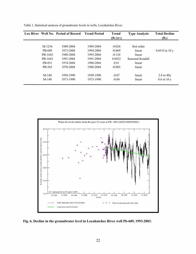
Table 1. Statistical analysis of groundwater levels in wells, Loxahatchee River.
Lox River Well No. Period of Record Trend Period Trend Type Analysis Total Decline(ft./yr.) (ft.)
M-1234 1988-2004 1989-2004 -0.024 first orderPB-689 1973-2004 1994-2004 -0.069 linear 0.69 ft in 10 y
PB-1642 1988-2004 1993-2004 -0.124 linearPB-1662 1991-2004 1991-2004 0.0422 Seasonal KendallPB-831 1974-2004 1980-2004 0.01 linearPB-565 1970-2004 1980-2004 -0.005 linear
M-140 1950-1990 1950-1990 -0.07 linear 2.8 in 40yM-140 1973-1990 1973-1990 -0.04 linear 0.6 in 16 y
Fig. 6. Decline in the groundwater level in Loxahatchee River well Pb-689, 1993-2003.
22
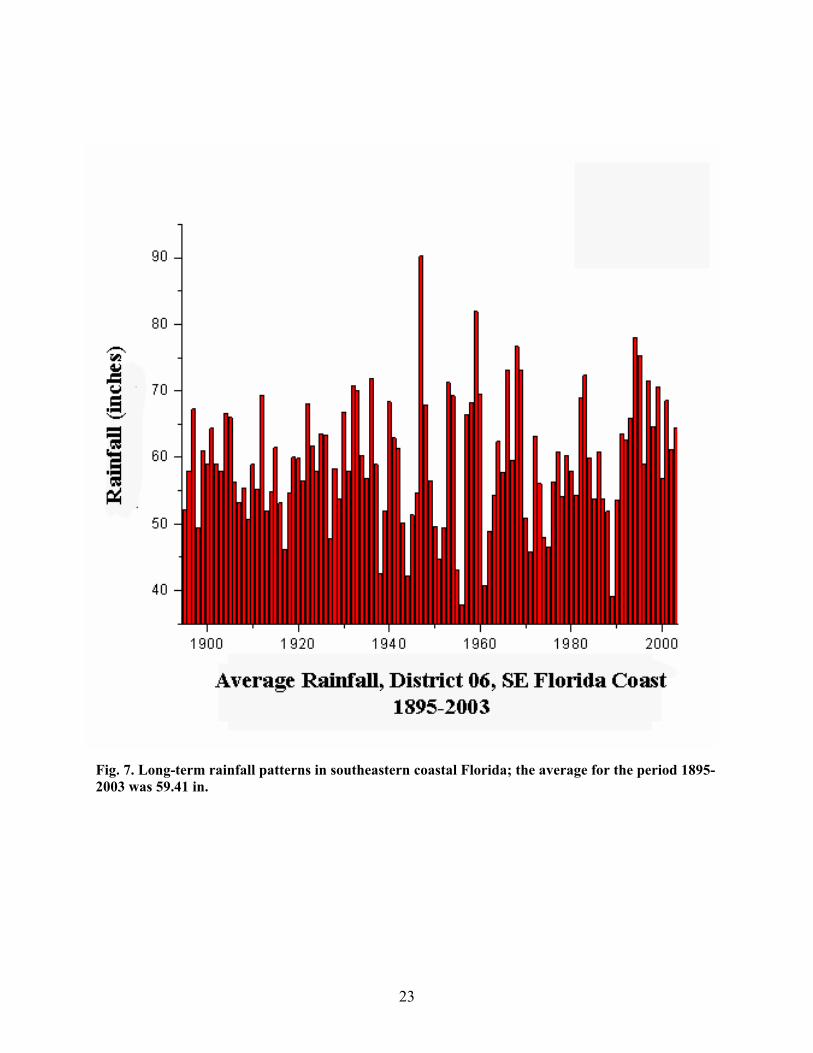
Fig. 7. Long-term rainfall patterns in southeastern coastal Florida; the average for the period 1895-2003 was 59.41 in.
23
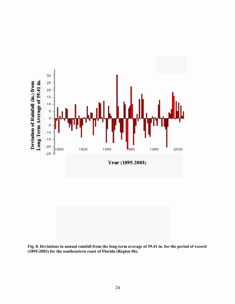
Fig. 8. Deviations in annual rainfall from the long-term average of 59.41 in. for the period of record (1895-2003) for the southeastern coast of Florida (Region 06).
24
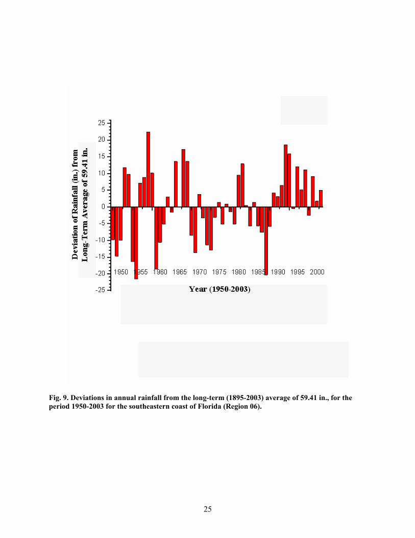
Fig. 9. Deviations in annual rainfall from the long-term (1895-2003) average of 59.41 in., for the period 1950-2003 for the southeastern coast of Florida (Region 06).
25
II.D. Long-Term Patterns in Floodplain Vegetation
Vegetative land cover in the vicinity of the Northwest Branch/Fork of the Loxahatchee River is
characterized by pine forest, wet prairie, or hardwood swamps, and mangrove forests along tributaries.
Freshwater hardwood swamps, of cypress, red maple, water oak, willow, bay trees and other hardwoods,
grow along upstream tributaries. Mangrove forest (with three species of mangrove) grows along
downstream tributaries, and mixes with hardwood trees along a transitional zone.
Hedgepeth and others (SFWMD, 2002) used existing historical aerial photography (1940, 1953,
1964, 1979, 1985, and 1995) to compare spatial and temporal changes in distribution and abundance of
vegetative communities along the floodplain of the Northwest Branch/Fork of the Loxahatchee River, and
to document changes in vegetation cover and correlate those changes to major events in the watershed.
The total vegetative community coverage by type and by year was compared over time to quantify
changes over the 55-year period 1940-1995. Over this time span, the wetland vegetative communities
declined in acreage as a result of several causes, including scouring of river bed, bulkheading,
development, and loss of wetland plants to transitional and upland species, as a result of flow diversions
and decreasing water levels. In the lower reach, mangrove forest was displaced by urbanization, but
overall mangrove forest coverage increased as it encroached upstream into predominately freshwater
communities. Along the middle stretches of the river, nine miles upstream of Jupiter Inlet, there was an
apparent increase in the number of plant species and a loss of cypress dominance. Along this intermediate
portion of the river and downstream, cypress trees show increasing stress and many trees have died. Such
changes in the freshwater vegetative communities may be due to impacts of saltwater intrusion and
decreased flows of fresh surface and groundwater inflows. Changes in freshwater habitat along the
Northwest Branch/Fork may be attributed to dredging of the Intracoastal Waterway (early 1900’s),
dredging downstream segments of the Loxahatchee River (1930’s), permanent opening of the Jupiter inlet
(1947), lowering of the freshwater table, and diversions of freshwater from the Northwest Branch/Fork
(1950’s). All these projects had a potential to allow increased upstream encroachment of seawater during
tidal cycles.
III. Study Area and Sampling
III.A. General Description
The study area includes the entire Loxahatchee River watershed for the historical data review and the
evaluation of historic groundwater levels for wells, while field studies focused primarily on the Northwest
Branch/Fork of the Loxahatchee River (Fig. 1), its floodplain and nearby uplands, and the estuary. The
26
study included two sampling periods, one during the wet season (September 2003) and one in the dry
season (March 2004).
The 699 km2 Loxahatchee River watershed provides water for three principal distributaries, the
Northwest Branch/Fork, and North- and Southwest Forks that discharge through Jupiter Inlet to the
Atlantic Ocean (Russell and McPherson, 1984). Natural and anthropogenic change in the watershed since
the 1940’s has resulted in increased saltwater intrusion up the Loxahatchee River estuary, and consequent
dramatic ecosystem change (McPherson et al., 1982; Noel et al., 1995). Compounding the issue of
saltwater intrusion may be a gradual decrease in available fresh surface- and groundwater, due to regional
construction of extensive canal networks for expansive urban growth centered around Jupiter, FL
(McPherson and Sonntag, 1984).
The lower Loxahatchee River estuary is mostly shallow (average depth ~ 1.2 m), although a partially
dredged and natural channel 3+ m deep extends about 14 km upstream. In the upper reaches of the river,
water depths are generally less than 2-3 m. The tides in the estuary are mixed-semi-diurnal, and the tidal
range is <1 m. A typical tidal wave may propagate upstream for about 16 km (Russell and Goodwin,
1987) at a rate of 8-16 km hr-1.
Freshwater inflows to the Loxahatchee River estuary may include local and regional upward
groundwater flow, precipitation, surface-water runoff, storm drainage and canal discharge. This
composite inflow, which is seasonal in nature and can be partially regulated during wet (May-November)
months, may have a strong tropical weather imprint (e.g., two hurricanes made landfall very close to the
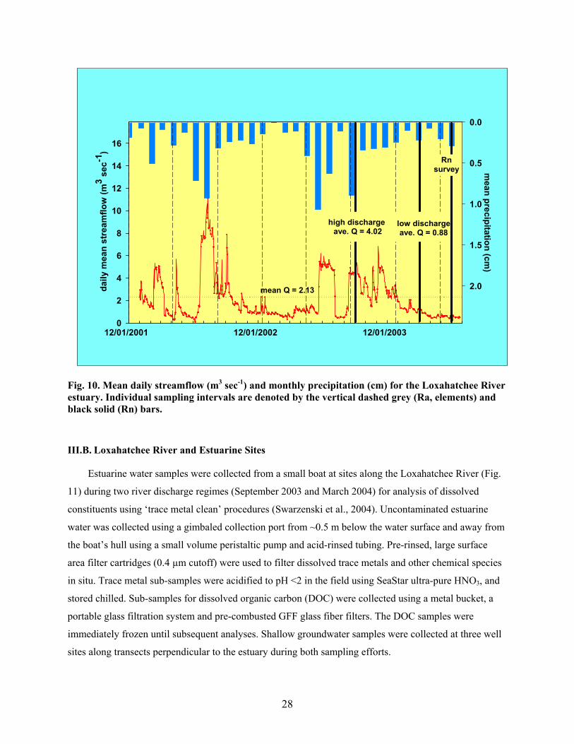
estuary in September 2004). Mean monthly precipitation rates at SFWMD Station No. C18W_R (26° 52’
19” N, 80° 14’ 42” W), and daily mean stream-flow upstream of the Northwest Branch/Fork of the
Loxahatchee River are illustrated in Fig. 10. This two plus-year record suggests a reasonably strong
relation between precipitation and stream flow. Average daily discharge rates for the upper Northwest
Branch/Fork of the Loxahatchee River (USGS site ID: 2277600; 26° 56’ 20” N, 80° 10’ 31” W) during
the high and low discharge sampling cruises were 4.02 and 0.88 m3 sec-1, respectively. A 2-yr mean
stream flow rate during the two sampling efforts was 2.15 m3 sec-1. For comparison, an average discharge
rate of about 300 m3 sec-1 has been reported for Jupiter Inlet (Mehta et al., 1992).
Groundwater/surface water interactions are often enhanced in carbonate-dominated coastal margins
and wetlands of Florida (Parker et al., 1955; Krest and Harvey, 2003). Biogeochemical transport in the
Loxahatchee River estuary was, therefore, investigated from the perspective that groundwater discharge
could play an important role in geochemical and water budgets of this estuarine system. Consequently,
the following discussion will develop in two directions: (1) traditional biogeochemical transformations
along salinity gradients, and (2) the role of groundwater discharge in impacting estuarine transport.
27
12/01/2001 12/01/2002 12/01/2003
daily
mea
n st
ream
flow
(m3 s
ec-1
)
0
2
4
6
8
10
12
14
16
mean precipitation (cm
)
0.0
0.5
1.0
1.5
2.0mean Q = 2.13
high discharge ave. Q = 4.02
low dischargeave. Q = 0.88
Rnsurvey
Fig. 10. Mean daily streamflow (m3 sec-1) and monthly precipitation (cm) for the Loxahatchee River estuary. Individual sampling intervals are denoted by the vertical dashed grey (Ra, elements) and black solid (Rn) bars.
III.B. Loxahatchee River and Estuarine Sites
Estuarine water samples were collected from a small boat at sites along the Loxahatchee River (Fig.
11) during two river discharge regimes (September 2003 and March 2004) for analysis of dissolved
constituents using ‘trace metal clean’ procedures (Swarzenski et al., 2004). Uncontaminated estuarine
water was collected using a gimbaled collection port from ~0.5 m below the water surface and away from
the boat’s hull using a small volume peristaltic pump and acid-rinsed tubing. Pre-rinsed, large surface
area filter cartridges (0.4 µm cutoff) were used to filter dissolved trace metals and other chemical species
in situ. Trace metal sub-samples were acidified to pH <2 in the field using SeaStar ultra-pure HNO3, and
stored chilled. Sub-samples for dissolved organic carbon (DOC) were collected using a metal bucket, a
portable glass filtration system and pre-combusted GFF glass fiber filters. The DOC samples were
immediately frozen until subsequent analyses. Shallow groundwater samples were collected at three well
sites along transects perpendicular to the estuary during both sampling efforts.
28
Low discharge sitesHigh discharge sitesStream guage
0 1 2 3 4 50.5Kilometers
StudyArea
Southwest Fork
80 9'23"W 80 7'30"W 80 5'38"W
26 56'15"N
26 58'8"N
27 0'0"N
27 1'53"N
0 0 0
0
0
0
0
AtlanticOcean
Northwest Fork
Loxahatchee River estuary
Jupiter
Kitching Creek
Fig. 11. Station location map for high (September 2003) and low (March 2004) discharge sampling efforts.
Samples for all four radium isotopes (223,224,226,228Ra) were collected (using the same gimbaled arm
and a 12v submersible pump) by passing a known volume of estuarine water through either 1 or 2 MnO2
impregnated acrylic fiber cartridges (Weiss et al., 1984). Two serial cartridges were used sporadically to
evaluate the Ra extraction efficiency onto the MnO2 fiber (typically >96 %). Target salinities and water
characteristics (e.g., temperature, pH, dissolved oxygen, specific conductivity, and salinity) were
29
continuously monitored during pumping operations with a multi-parameter YSI probe. The suspended
particulate matter (SPM) concentration per sample was determined gravimetrically in the lab, using pre-
weighed 0.4 µm Nuclepore filters (47 mm diameter).
Near-continuous excess radon-222 activities were measured in the Loxahatchee River estuary in
June 2004 using six commercial air radon detectors (RAD7 – Durridge, Co., Inc.), routed simultaneously
through a single air-water exchanger (Burnett et al., 2001). By applying a temperature and solubility
coefficient correction, one can calculate the activity of 222Rn in water, as the Rn in air will attain
equilibrium with estuarine water flowing through the exchanger after about 20 min. Utilizing six RAD7
detectors simultaneously permits almost real-time (once every 5-min) Rn data acquisition. During this
survey, water column characteristics were again monitored both at the exchanger site and within the water
column using an in situ multi-parameter sensor array, as well as WTW multi-probes.
To physically validate the Ra-derived groundwater flux rate for the estuary, direct seepage across the
sediment/water interface was measured during the high discharge sampling cruise in September, 2003 at
Kitching Creek (Fig 11), using an autonomous electromagnetic seepage meter (Rosenberry and Morin,
2004; Swarzenski et al., 2004b). A streaming resistivity profiling survey (Manheim et al., 2002; Belaval
et al., 2003; Swarzenski et al., 2004d) was also conducted in this estuary during the June 2004 field effort
to provide detailed information on the dynamic subsurface freshwater/saltwater interface of this estuary.
III.C. Loxahatchee River Floodplain Sites
In addition to studies conducted in the Loxahatchee River Estuary, surveys of vegetation, and
measurements of geochemical parameters in the floodplain surface water and porewater were also
conducted during the same wet and dry period cycles (September 2003 and March 2004). In 2003, the
SFWMD and the Florida Park Service established vegetation monitoring studies for plant community
composition and structure in order to document baseline and future plant community health along the
floodplains of the North Fork and Northwest Branch/Fork of the Loxahatchee River and Kitching Creek.
The project examined vegetation along six historical transects and established four new transects in areas
of concern (Fig. 12). The transects are located in areas representative of riverine (predominantly non-
impacted freshwater), and upper tidal (saltwater intruded with fresh and brackish water) communities.
Seven transects were established at designated locations along the middle and upper segments of the
Northwest Branch/Fork of the Loxahatchee River. Additional transects were established in the lower
segment of Kitching and Cypress Creeks (tributaries of the Northwest Fork), and in the upper North Fork
of the Loxahatchee River.
Surface water, porewater, and sediment samples were collected at points located along transects 1,
30
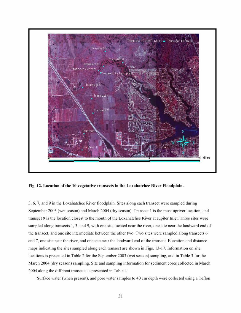
Fig. 12. Location of the 10 vegetative transects in the Loxahatchee River Floodplain.
3, 6, 7, and 9 in the Loxahatchee River floodplain. Sites along each transect were sampled during
September 2003 (wet season) and March 2004 (dry season). Transect 1 is the most upriver location, and
transect 9 is the location closest to the mouth of the Loxahatchee River at Jupiter Inlet. Three sites were
sampled along transects 1, 3, and 9, with one site located near the river, one site near the landward end of
the transect, and one site intermediate between the other two. Two sites were sampled along transects 6
and 7, one site near the river, and one site near the landward end of the transect. Elevation and distance
maps indicating the sites sampled along each transect are shown in Figs. 13-17. Information on site
locations is presented in Table 2 for the September 2003 (wet season) sampling, and in Table 3 for the
March 2004 (dry season) sampling. Site and sampling information for sediment cores collected in March
2004 along the different transects is presented in Table 4.
Surface water (when present), and pore water samples to 40 cm depth were collected using a Teflon
31
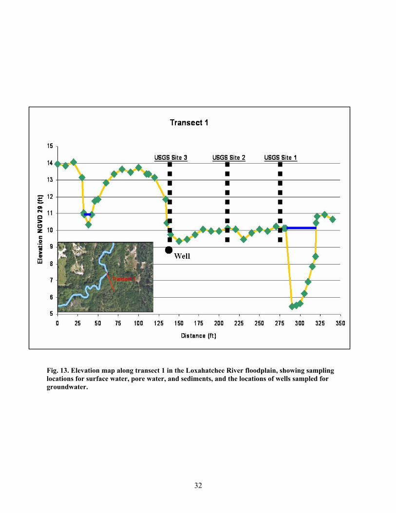
Fig. 13. Elevation map along transect 1 in the Loxahatchee River floodplain, showing sampling locations for surface water, pore water, and sediments, and the locations of wells () sampled for groundwater.
Fig. 13. Elevation map along transect 1 in the Loxahatchee River floodplain, showing sampling locations for surface water, pore water, and sediments, and the locations of wells sampled for groundwater.
32
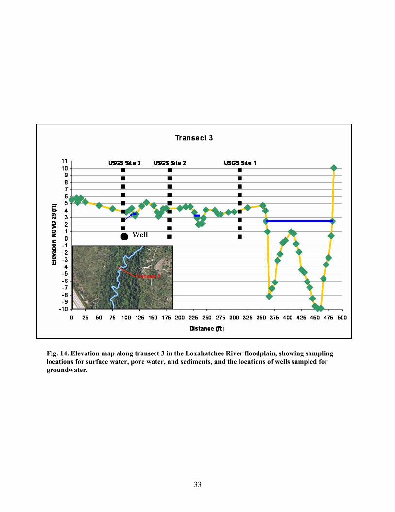
Fig. 14. Elevation map along transect 3 in the Loxahatchee River floodplain, showing sampling locations for surface water, pore water, and sediments, and the locations of wells sampled for groundwater.
33
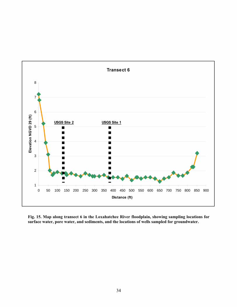
Transect 6
1
2
3
4
5
6
7
8
0 50 100 150 200 250 300 350 400 450 500 550 600 650 700 750 800 850 900
Distance (ft)
Elev
atio
n N
GVD
29
(ft)
USGS Site 1USGS Site 2
Fig. 15. Map along transect 6 in the Loxahatchee River floodplain, showing sampling locations for surface water, pore water, and sediments, and the locations of wells sampled for groundwater.
34
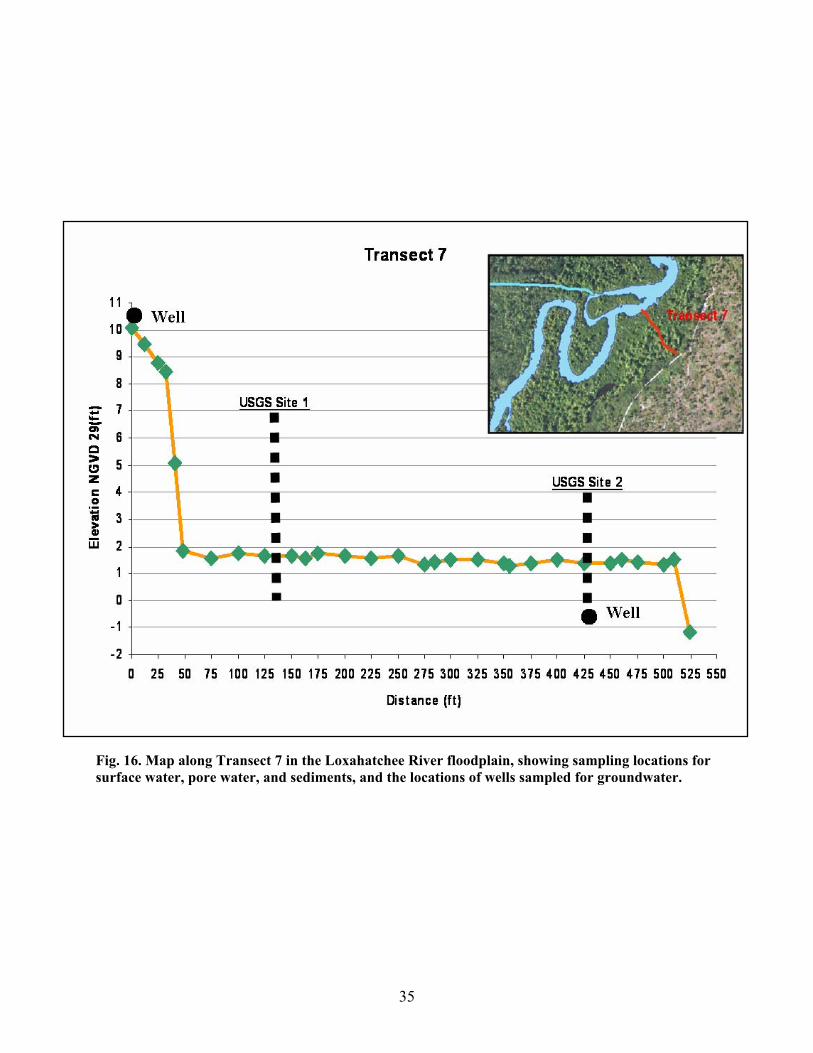
Fig. 16. Map along Transect 7 in the Loxahatchee River floodplain, showing sampling locations for surface water, pore water, and sediments, and the locations of wells sampled for groundwater.
35
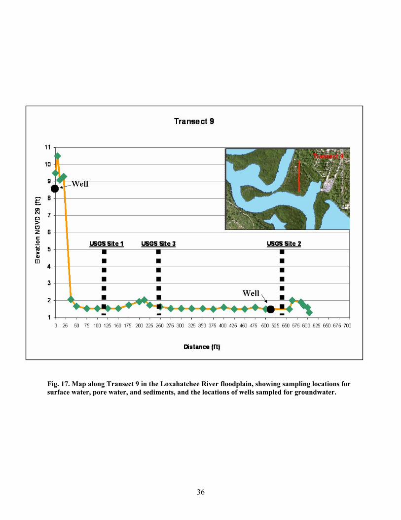
Fig. 17. Map along Transect 9 in the Loxahatchee River floodplain, showing sampling locations for surface water, pore water, and sediments, and the locations of wells sampled for groundwater.
36
micropiezometer probe connected via Teflon tubing to an inline filter (1.0 µm GF/C) and a battery-
powered, field-portable pump (geopump). A smaller diameter stainless steel micropiezometer, operated in
the same manner as the Teflon micropiezometer, was used to collect deeper pore water to a depth of 80
cm. Surface water was collected first at each site using the Teflon micropiezometer and pump. Collecting
surface water first minimizes cross contamination issues, since surface water typically has lower
concentrations of dissolved chemical species than porewater. A minimum of 100 ml of surface water was
flushed through the micropiezometer setup prior to collection of sample in order to minimize
contamination. Porewater was collected at 5 different depth intervals at most sites (Tables 2 and 3).
Depths of 2, 5, 10, 20, and 40 cm were the target intervals for porewater sampling, but dry conditions near
the sediment surface (especially along Transects 1 and 3 in March 2004), and a layer of highly compacted
sediment below 20 cm at some sites limited water flow to the micropiezometer, and prevented collection
of pore water samples from some depths at some sites. Pore water samples from depths >40 cm were
collected at selected sites (Table 3) during March 2004, after it became apparent from the September
2003 sampling that higher ionic strength water was present at depth.
Water samples from wells located along transects 1, 3, 7, and 9 were also collected (Tables 2 and 3)
using Teflon or plastic tubing connected to an inline filter (1.0 µm GF/C), and the portable field pump
(geopump).
Sediment cores were collected at selected locations along transects 1, 3, 6, 7, and 9 (Table 4). The
cores were collected using a custom piston corer with plexiglas core tube, PVC piston, and stainless steel
cutter and adjustable handles. The coring device is a smaller variation of a piston corer used in the
Everglades (Orem et al., 1997). The core tube is 2.5 inches in diameter and about 4 feet long, which
provides sufficient material for chemical analyses, but makes the corer relatively easy to carry along the
heavily forested, flooded transects.
Cores were collected in a manner similar to that described in Orem et al. (1997): connecting the
piston to a small monopod using stainless steel cable, positioning the piston at the sediment surface in the
core tube, and pushing the core tube into the sediment (piston remaining stationary at the sediment
surface) using the adjustable stainless steel handles clamped to the core tube. Cores were retrieved by
securing the piston around the handles using the stainless steel cable to maintain it in place, and manually
pulling the core barrel out of the sediment using the handles (Orem et al., 1997). Cores were capped in the
field, and transported upright to a convenient area (hotel parking lot) for extrusion and sampling.
Cores were extruded vertically, sectioned every 2 cm, and each section placed into a labeled plastic
zip-lock bag. Sediment samples in zip-lock bags were frozen on dry ice, and shipped to laboratory
facilities at the USGS in Reston, VA. At the lab, sediments were lyophilized, ground to a powder, and
stored in glass vials prior to analysis.
37
Tabl
e 2.
Tra
nsec
t and
site
info
rmat
ion
for w
et se
ason
sam
plin
g, L
oxah
atch
ee R
iver
, Flo
rida,
Sep
tem
ber 1
5-18
, 200
3.
22
2T
rans
ect
Dat
eSi
teM
arke
r1,2
Lat
.2L
ong.
Pore
wat
er D
epth
sN
otes
(m)
(cm
)1
9/15
/200
31
8526
56.
410N
80 1
0.36
2Wsw
, 2, 5
, 10,
20,
34.
59/
15/2
003
265
26 5
6.41
7N80
10.
350W
sw, 2
, 5, 1
0, 2
0, 3
59/
15/2
003
340
26 5
6.40
8N80
10.
338W
sw, 2
, 5, 1
0, 2
0, 3
79/
15/2
003
wel
l35
26 5
6.40
6N80
10.
335W
wel
l wat
er
39/
16/2
003
195
26 5
7.72
9N80
09.
918W
sw, 2
, 5, 1
0, 2
0, 2
3di
ffic
ult p
umpi
ng p
orew
ater
at >
23 c
m9/
16/2
003
255
26 5
7.67
8N80
09.
891W
sw, 2
, 5, 1
0, 2
0, 2
3.5
diff
icul
t pum
ping
por
ewat
er a
t >23
cm
9/16
/200
33
3026
57.
670N
80 0
9.87
5Wsw
, 2, 5
, 10
sand
bel
ow 1
0 cm
9/16
/200
3w
ell
3026
57.
670N
80 0
9.87
5Ww
ell w
ater
69/
17/2
003
111
526
59.
320N
80 0
9.40
7Wsw
, 2, 5
, 10,
20,
34
9/17
/200
32
4026
59.
285N
80 0
9.40
4Wsw
, 2, 5
, 10,
20,
40.
5
79/
16/2
003
140
26 5
9.05
7N80
09.
544W
sw, 2
, 5, 1
0, 2
0, 4
1co
llect
ed d
urin
g flo
od ti
de9/
17/2
003
213
026
59.
097N
80 0
9.57
3Wsw
, 2, 5
, 10,
20,
34
colle
cted
dur
ing
ebb
tide
9/16
/200
3w
ell #
10
26 5
9.03
9N80
09.
533W
wel
l wat
erco
llect
ed d
urin
g flo
od ti
de9/
17/2
003
wel
l #2
130
26 5
9.09
7N80
09.
573W
wel
l wat
erco
llect
ed d
urin
g eb
b tid
e
99/
18/2
003
135
26 5
9.35
2N80
08.
642W
sw, 2
, 5, 1
0, 2
0, 4
09/
18/2
003
216
526
59.
288N
80 0
8.64
5Wsw
, 2, 5
, 10,
20,
35
9/18
/200
33
7526
59.
288N
80 0
8.64
5Wsw
, 2, 5
, 10,
20
9/18
/200
3w
ell #
10
26 5
9.37
2N80
08.
640W
wel
l wat
eron
slop
e ab
ove
trans
ect
9/18
/200
3w
ell #
215
526
59.
281N
80 0
8.64
5Ww
ell w
ater
1 - D
ista
nce
in m
from
beg
inni
ng o
f tra
nsec
t bas
ed o
n es
tabl
ishe
d tra
nsec
t dis
tanc
e m
arke
rs2
- Lat
. = la
titud
e; L
ong.
= lo
ngitu
de; c
m =
cen
timet
ers;
m =
met
ers;
sw =
surf
ace
wat
er; >
= g
reat
er th
an
38
Tabl
e 3.
Tra
nsec
t and
site
info
rmat
ion
for d
ry se
ason
sam
plin
g, L
oxah
atch
ee R
iver
, Flo
rida,
Mar
ch 8
-11,
200
4.
22
2T
rans
ect
Dat
eSi
teM
arke
r1,2
Lat
.2L
ong.
Pore
wat
er D
epth
sN
otes
(m)
(cm
)1
3/8/
2004
185
26 5
6.41
0N80
10.
362W
sw, 2
0, 4
0, 5
0Se
dim
ent d
ry a
bove
20
cm3/
8/20
042
6526
56.
417N
80 1
0.35
0W20
, 30,
40,
50,
60
Sedi
men
t dry
abo
ve 1
0 cm
3/8/
2004
340
26 5
6.40
8N80
10.
338W
20, 3
0. 4
0, 5
0, 6
0Se
dim
ent d
ry a
bove
10
cm3/
8/20
04w
ell
3526
56.
406N
80 1
0.33
5Ww
ell w
ater
33/
9/20
041
9526
57.
729N
80 0
9.91
8Wsw
, 5, 1
0, 2
0, 3
0Se
dim
ent d
ry/H
ighl
y co
lore
d po
rew
ater
3/9/
2004
255
26 5
7.67
8N80
09.
891W
20, 2
9Se
dim
ent d
ry/H
ighl
y co
lore
d po
rew
ater
3/9/
2004
330
26 5
7.67
0N80
09.
875W
sw, 1
0, 2
0Se
dim
ent d
ry/H
ighl
y co
lore
d po
rew
ater
3/9/
2004
wel
l30
26 5
7.67
0N80
09.
875W
wel
l wat
er
63/
10/2
004
111
526
59.
320N
80 0
9.40
7Wsw
, 2, 5
, 10,
20,
40
3/10
/200
42
4026
59.
285N
80 0
9.40
4Wsw
, 2, 5
, 10,
20,
40
73/
9/20
041
4026
59.
057N
80 0
9.54
4W2,
5, 1
0, 2
0, 4
0N
o sw
pre
sent
3/9/
2004
213
026
59.
097N
80 0
9.57
3Wsw
, 2, 5
, 10,
20,
34
3/9/
2004
wel
l #1
026
59.
039N
80 0
9.53
3Ww
ell w
ater
3/9/
2004
wel
l #2
130
26 5
9.09
7N80
09.
573W
wel
l wat
er
93/
11/2
004
135
26 5
9.35
2N80
08.
642W
sw, 1
0, 2
0, 4
0, 6
0, 8
43/
10/2
004
2LT
165
26 5
9.28
8N80
08.
645W
sw, 2
, 5, 1
0, 2
0, 4
0, 6
0, 8
0Lo
w ti
de sa
mpl
e - s
ite 2
3/11
/200
42H
T16
526
59.
288N
80 0
8.64
5Wsw
, 5, 2
0, 4
0, 8
0H
igh
tide
sam
ple
- site
23/
11/2
004
375
26 5
9.32
9N80
08.
645W
sw, 2
, 5, 1
0, 2
0, 4
0, 6
0, 8
03/
11/2
004
wel
l #1
026
59.
372N
80 0
8.64
0Ww
ell w
ater
3/10
/200
4w
ell #
215
526
59.
281N
80 0
8.64
5Ww
ell w
ater
1 - D
ista
nce
in m
from
beg
inni
ng o
f tra
nsec
t bas
ed o
n es
tabl
ishe
d tra
nsec
t dis
tanc
e m
arke
rs2
- Lat
. = la
titud
e; L
ong.
= lo
ngitu
de; c
m =
cen
timet
ers;
m =
met
ers;
sw =
surf
ace
wat
er; >
= g
reat
er th
an
39
Tabl
e 4.
Tra
nsec
t and
site
info
rmat
ion
for s
edim
ent c
orin
g, L
oxah
atch
ee R
iver
, Flo
rida,
Mar
ch 8
-11,
200
4.
22
3T
rans
ect
Dat
eSi
teM
arke
r1,2
Lat
.L
ong.
Sedi
men
t Cor
es2
Com
pact
ion
(m)
(%)
13/
8/20
041
8526
56.
410N
80 1
0.36
2W23
cm
cor
e/46
cm
hol
e50
3/8/
2004
265
26 5
6.41
7N80
10.
350W
33 c
m c
ore/
48 c
m h
ole
313/
8/20
043
4026
56.
408N
80 1
0.33
8W26
cm
cor
e/53
cm
hol
e51
33/
9/20
041
9526
57.
729N
80 0
9.91
8W56
cm
cor
e/67
cm
hol
e16
3/9/
2004
255
26 5
7.67
8N80
09.
891W
20 c
m c
ore/
30 c
m h
ole
333/
9/20
043
3026
57.
670N
80 0
9.87
5W26
cm
cor
e, 4
3 cm
hol
e40
63/
10/2
004
111
526
59.
320N
80 0
9.40
7W24
cm
cor
e/72
cm
hol
e67
3/10
/200
42
4026
59.
285N
80 0
9.40
4W20
cm
cor
e/71
cm
hol
e72
73/
9/20
041
4026
59.
057N
80 0
9.54
4W31
cm
cor
e/34
cm
hol
e9
3/9/
2004
213
026
59.
097N
80 0
9.57
3W22
cm
cor
e/61
cm
hol
e64
93/
11/2
004
135
26 5
9.35
2N80
08.
642W
18 c
m c
ore/
75 c
m h
ole
763/
10/2
004
216
526
59.
288N
80 0
8.64
5W22
cm
cor
e/78
cm
hol
e72
3/11
/200
43
7526
59.
329N
80 0
8.64
5W15
cm
cor
e/35
cm
hol
e57
1 - D
ista
nce
in m
from
beg
inni
ng o
f tra
nsec
t bas
ed o
n es
tabl
ishe
d tra
nsec
t dis
tanc
e m
arke
rs2
- Lat
. = la
titud
e; L
ong.
= lo
ngitu
de; c
m =
cen
timet
ers;
m =
met
ers;
sw =
surf
ace
wat
er; >
= g
reat
er th
an3
- % C
ompa
ctio
n ca
lcul
ated
as f
ollo
ws:
[(le
ngth
of c
ore)
/(dep
th o
f cor
e ho
le)]
x 1
00
40
IV. Methods
IV.A. Groundwater Flux Measurements
Groundwater fluxes were evaluated using isotopic tracers as described by Swarzenski (1999).
Freshwater-saltwater interface processes were examined with four radium isotopes (USGS Fact Sheet FS-
065-99), similar to the multiple geochemical tracer approach used to characterize the hydrogeology of the
submarine spring off Crescent Beach, Florida (Swarzenski et al., 2001).
There are four radium isotopes in the 238U, 232Th and 235U decay series; their individual half-lives
(223Ra: t½ = 11.4 d, 224Ra: t½ = 3.6 d, 228Ra: t½ = 5.7 yr and 226Ra: 1600 yr) make them ideally suited to
study many aquatic processes that occur over time scales of days to years. Strongly particle-reactive
thorium isotopes (Th half-lives range from days to 1 x10¹⁰ yr) decay to form radium isotopes. In
freshwater, radium as a Group IIA alkaline–earth metal is also strongly bound onto particle surfaces. As
these Ra-surface sites become exposed to higher ionic strength groundwater or seawater, Ra undergoes a
rapid phase transformation and resides exclusively as a dissolved species. Thorium, in contrast, will
continue to remain bound onto particles regardless of salinity, and will continuously generate radium.
Sediments thus provide a constant source of Ra to the overlying waters, and the production rate is defined
directly by the particular isotope’s decay constant. Radium isotopes, therefore, provide an invaluable
means for assessing the exchange of water across the sediment-water interface (Swarzenski et al., 1998)
In the Loxahatchee River system, where the underlying sediments are flushed either continuously or
sporadically by groundwater, a localized disequilibrium between 228Th and 228Ra will develop. This
occurs because Ra is rapidly released into the water column while thorium remains attached to the bottom
sediments. One can use this disequilibrium to derive a groundwater flux rate (water mass mixing rate).
Assuming steady state conditions, the flux of 228Ra from the surface sediments will deplete the activities
of its progeny, 228Th and 224Ra. Below this active surface sediment layer, one can expect secular
equilibrium from 232Th down to 224Ra, which takes about 20 years. Bioturbation as well as groundwater
flow will facilitate the interaction of these two sediment layers, causing an upward flux of 228Ra, and 224Ra. Radium isotopes removed from the surface sediment layer by upward groundwater discharge will,
thus, provide information on the rate of groundwater discharge across the sediment water interface and
will also provide insight on the relative contribution of groundwater to the overall movement of surface
water through the Loxahatchee River system.
Marine geochemists have been able to clearly demonstrate that 228Ra/226Ra activity ratios can be an
ideal tracer for water mass migration studies (Porcelli and Swarzenski, 2003). Unlike other tracers that may
not be conservative or easily quantifiable, the 228Ra/226Ra activity ratio is not modified by evaporation,
precipitation, or biological activity, dependent only on radioactive decay. Because of the relatively long
half-life of 228Ra and 226Ra, these two isotopes are not too useful for determining mixing rates/processes on
41
time scales of a few days to weeks. The shorter-lived radium isotopes 223Ra and 224Ra are, however, ideal to
examine weekly events and can be applied with similar success.
IV.B. Groundwater Flux Calculations
To use the activity of excess 224Ra in a water sample as a geochronometer for water movement or
transport (residence times), a mass balance equation is written as follows: 224Raobs = 224RaiƒEMe-λ224t
and solving for time t:
t = -ln [224Raobs / 224RaiƒEM] / λ224
where λ224 is the decay constant for 224Ra (0.189 days-1), 224Rai is the initial amount of 224Ra in the water
sample, 224Raobs is the observed (measured) 224Ra in the water sample, and ƒEM is the fraction of the end
member (well sample) remaining in the sample. Age determinations calculated in such a manner reflect
the time elapsed since the water sample became enriched in Ra by the discharge of groundwater. 224Ra is
regenerated on the order of days. The fraction ƒEM can be estimated either from the salinity signal or from
the distribution of 228,226Ra isotopes, but this term can be difficult to constrain in non-two endmember
systems. One can write a similar equation describing the change in activity as a result of mixing and
decay for 223Ra and dividing this by the above equation yields: (ƒEM drops out):
[223Ra/224Ra]obs = [223Ra/224Ra]i [e-λ223t/e-λ224t]
This equation should be useful for Loxahatchee River waters because the term ƒem is removed. Using 223Ra/224Ra isotope ratios in this manner is based on the assumption that the initial 223Ra/224Ra activity ratio
must remain constant. This is a reasonable assumption since the long-lived parent isotopes (231Pa and 232Th)
have relatively constant activity ratios in sediments, and the intermediate Th isotopes (227Th and 228Th) are
scavenged efficiently in the near-shore water column, as field tested and verified by Swarzenski and others
(2003).
Radon-222 has been proven effective as a tracer of subsurface discharge to the ocean in karst ground
water systems (Cable et al., 1996, 1997). In addition, activity ratios between 222Rn and 224Ra have
indicated that unique water mass sources can be identified flowing into the near shore northeastern Gulf
of Mexico (Cable and Moore, personal communication). The mass balance technique is based on
measurement of the radon sources and sinks activities to obtain the groundwater derived radon component
as shown:
Cf = [νsCn-1Ao + Jben + (λCRa)Vn]/[νsAn+1 + λVn]
where Cf is the final 222Rn activity exiting the transect in a horizontal plane; Cn-1 is the 222Rn activity
entering each volume increment along the transect for n increments; νs is the velocity of the surface water
along the transect; An is the area at the initial side of each increment (sampling station); Jben is the benthic
42
input of radon to the surface waters; λ is the 222Rn decay constant (1.25 x 10⁻⁴ min-1); λCRa represents the
water column radon production; Vn is the volume of water in individual segments of the transect; and An+1
is the area of the exit (inshore) side of the nth increment. For a region where both the volume of surface
water flow and groundwater flow are unknown, it is important to measure one before using this mass
balance. This proposed study would assess the radon activities in the ground water. In this way, the mass
balance can be solved iteratively by changing the surface water volume term until the radon budget yields
a Cf similar to what is observed in the field.
IV.C. Analytical Methods for Chemical Species
IV.C.1. River and estuarine water column samples - River and estuarine water samples were
analyzed for dissolved trace elements by isotope dilution inductively coupled plasma mass spectrometry.
Reported detection limits (in µg L-1) for the suite of trace elements are as follows: Si (50), U (0.001), V
(0.05), Mn (0.05), Fe (5), Co (0.005), Sr (0.04), and Ba (0.1). Dissolved organic carbon (DOC)
concentrations were quantified by high-temperature catalytic oxidation, using a Shimadzu TOC 5000
analyzer. 223,224Ra activities (t½ = 11.4 d and 3.7 d, respectively) were determined using delayed
coincidence alpha counting techniques (Moore and Arnold, 1996; Swarzenski et al., 2001; Charette and
Buessler, 2004), while the two longer-lived Ra isotopes (228,226Ra – t1/2 = 5.7 y and 1620 y, respectively)
were subsequently extracted quantitatively from the MnO2 fiber and analyzed using peak energies by
high-resolution gamma spectroscopy with a well-type configuration (Kim and Burnett, 1983). The short-
lived Ra isotopes were recounted after ~3 weeks to correct for supported 224Ra activities (228Th), decay-
corrected to the sampling time, and propagated errors were typically <10 %. Aqueous 222Rn activities
were quantified using multiple RAD7 detectors routed through a single air-water exchanger (Burnett et
al., 2001; Burnett and Dulaiova, 2003).
Trade names are used in this report for descriptive purposes only; no endorsement of products by the
U.S. Geological Survey is implied.
IV.C.2. Floodplain surface and pore water samples - Surface water and porewater samples from
the Loxahatchee River floodplain were analyzed for the following parameters: redox, pH, titration
alkalinity, conductivity, salinity, total dissolved solids, nutrients (nitrate, ammonium, and phosphate),
anions (chloride, fluoride, bromide, and sulfate), sulfide, and major cations (sodium, potassium, calcium,
magnesium). A synopsis of methods used for surface and pore water chemical analysis is presented in
Table 5. Redox (calibrated with two point redox couple standard) was measured by electrode in the field
immediately after collection of sample from the micropiezometer into a syringe. Sample (3 ml) for sulfide
analysis was preserved in the field by addition of 3 ml of sulfur antioxidant buffer (SAOB) to the sample
in a small plastic container. Analysis of sulfide was carried out within 6-8 hours of collection in a hotel
43
room laboratory by sulfur electrode (sulfide electrode calibration is carried out just prior to a field trip).
pH and titration alkalinity were measured within 6-8 hours of sample collection in a hotel room
laboratory; pH using a semi-micro electrode and 2 point buffer calibration, and titration alkalinity by
addition of 0.1 M HCl with a micro burette to the sample with pH measurement. Conductivity, salinity,
and total dissolved solids measurements were carried out by electrochemical measurements within 6-8
hours of sample collection in hotel room laboratories. Samples for ammonium and phosphate analysis
were frozen on dry ice within 6-8 hours of collection, and transported to laboratory facilities (USGS Labs
in Reston, VA) for analysis using standard colorimetric methods. Anions and nitrate concentrations were
determined by suppressed anion chromatography, using dual detectors (conductivity for chloride,
fluoride, bromide, and sulfate; conductivity and uv/vis absorbance for nitrate). Major cation
concentrations (Na, K, Mg, Ca) were determined by suppressed cation chromatography with conductivity
detection. Identification and quantification of individual anions and cations was accomplished using
external calibration standards and peak area calculation using Waters Associates Millennium
chromatography software.
Percentage relative standard deviation (%RSD) for each procedure can vary somewhat from sample
to sample, however, average %RSD’s for each procedure are as follows: ± 10% for pH and titration
alkalinity, ± 20% for redox, ± 2% for conductivity, salinity, and total dissolved solids, ± 5% for
ammonium and phosphate, ±7% for sulfide, ± 4% for anion chromatography (including nitrate), and ± 7%
for cation chromatography. Conservative estimates of detection limits for each method are: 0.1 ppb for
sulfide, 0.05 mg/l for cations and anions (excluding major interferences), 0.5 µg/l for phosphate and
ammonium, 0.1 µS for conductivity, 0.1 ppt for salinity, and 0.1 mg/l for total dissolved solids.
IV.C.3. Floodplain sediment samples - Sediments samples (dried) were analyzed for total carbon
(TC), organic carbon (OC), total nitrogen (TN), total phosphorus (TP), and total sulfur (TS). All results
are reported on a sediment dry weight basis. TC, OC, TN, and TS contents of sediments were determined
using a Leco 932 CNS Analyzer (Leco Corporation, St. Joseph, MI, USA), as discussed by Orem et al.
(1999). TC, TN, and TS were measured directly, after drying the sediment overnight at 60° C. OC was
determined after removal of inorganic carbon using an acid vapor method slightly modified from that of
Hedges and Stern (1984), and Yamamuro and Kayanne (1995). Sediment samples (5 to 6 mg) were
weighed into prebaked (450° C) silver cups, placed in an acid vapor chamber (dessicator with beakers of
concentrated HCl in the bottom), allowed to react for a minimum of 48 hrs, dried (60° C), and analyzed.
Results showed virtually no inorganic carbon present in these cores, with TC and OC values virtually
identical. Therefore, only TC values are reported. All samples were analyzed at least in duplicate for all
parameters. Analytical precision (percentage relative standard deviation) was about 2% for TC, 4% for
OC, 3% for TN, and 5% for TS.
44
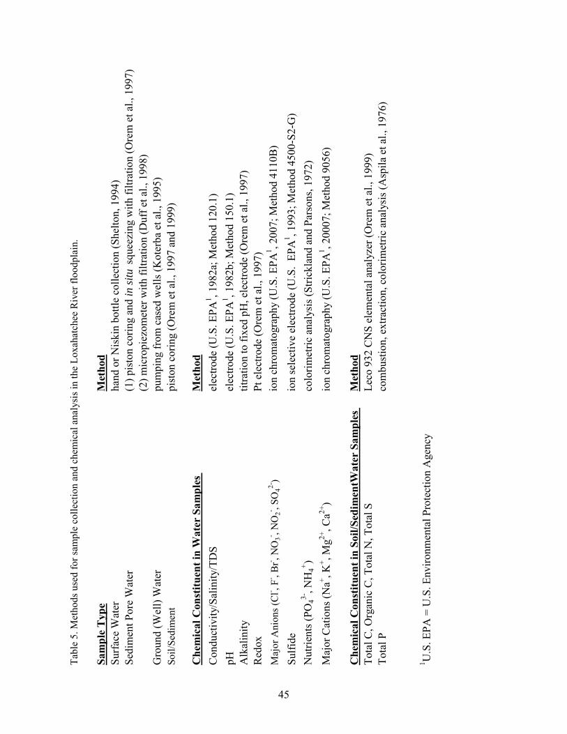
Tabl
e 5.
Met
hods
use
d fo
r sam
ple
colle
ctio
n an
d ch
emic
al a
naly
sis i
n th
e Lo
xaha
tche
e R
iver
floo
dpla
in.
Sam
ple
Typ
eM
etho
dSu
rfac
e W
ater
hand
or N
iski
n bo
ttle
colle
ctio
n (S
helto
n, 1
994)
Sedi
men
t Por
e W
ater
(1) p
isto
n co
ring
and
in si
tu s
quee
zing
with
filtr
atio
n (O
rem
et a
l., 1
997)
(2) m
icro
piez
omet
er w
ith fi
ltrat
ion
(Duf
f et a
l., 1
998)
Gro
und
(Wel
l) W
ater
pum
ping
from
cas
ed w
ells
(Kot
erba
et a
l., 1
995)
Soil/
Sedi
men
tpi
ston
cor
ing
(Ore
m e
t al.,
199
7 an
d 19
99)
Che
mic
al C
onst
ituen
t in
Wat
er S
ampl
es
Met
hod
Con
duct
ivity
/Sal
inity
/TD
Sel
ectro
de (U
.S. E
PA1 , 1
982a
; Met
hod
120.
1)pH
elec
trode
(U.S
. EPA
1 , 198
2b; M
etho
d 15
0.1)
Alk
alin
itytit
ratio
n to
fixe
d pH
, ele
ctro
de (O
rem
et a
l., 1
997)
R
edox
Pt e
lect
rode
(Ore
m e
t al.,
199
7)
2-)
Maj
or A
nion
s (C
l- , F- , B
r- , NO
3- , NO
2- , SO
4io
n ch
rom
atog
raph
y (U
.S. E
PA1 , 2
007;
Met
hod
4110
B)
Sulfi
deio
n se
lect
ive
elec
trode
(U.S
. EP
A1 , 1
993;
Met
hod
4500
-S2-
G)
+ )N
utrie
nts (
PO43-
, NH
4co
lorim
etric
ana
lysi
s (St
rickl
and
and
Pars
ons,
1972
) M
ajor
Cat
ions
(Na+ , K
+ , Mg2+
, Ca2+
)io
n ch
rom
atog
raph
y (U
.S. E
PA1 , 2
0007
; Met
hod
9056
)
Che
mic
al C
onst
ituen
t in
Soil/
Sedi
men
tWat
er S
ampl
es
Met
hod
Tota
l C, O
rgan
ic C
, Tot
al N
, Tot
al S
Leco
932
CN
S el
emen
tal a
naly
zer (
Ore
m e
t al.,
199
9)To
tal P
com
bust
ion,
ext
ract
ion,
col
orim
etric
ana
lysi
s (A
spila
et a
l., 1
976)
1 U.S
. EPA
= U
.S. E
nviro
nmen
tal P
rote
ctio
n A
genc
y
45
Total phosphorus (TP) concentrations in sediments were determined by the method of Aspila et al.
(1976), slightly modified for work in Loxahatchee River floodplain sediments. Samples were dried
overnight (60° C), cooled to room temperature in a desiccator, weighed, and placed in precleaned (soaked
in 10% HCl overnight, rinsed with deionized/distilled water, and baked at 450° C) ceramic crucibles.
Generally, 0.4-0.6 g of the sediment was used for TP analysis. Weighed sediment samples were baked at
550° C for 2 hrs., cooled, then transferred into clean plastic centrifuge cones containing 45 ml of 1 M
HCl. All plastic and glassware used for TP analysis was cleaned by soaking in 10% HCl overnight,
followed by rinsing with deionized/distilled water. The empty crucibles were rinsed with 5 ml of 1 M HCl
and the rinse was added to the centrifuge cones for a final volume of 50 ml of 1 M HCl. The samples
were extracted in the 1 M HCl for 16 hrs. on a shaker to dissolve the phosphate. An aliquot of each
extract was centrifuge filtered using Millipore ultrafree-CL HVPP low-binding Durapore centrifuge filters
(0.4 μm pore size), then neutralized with a NaOH solution, and transferred to plastic test tubes. The
filtered aliquots were analyzed for phosphate using the standard phospho-molybdate method (Strickland
and Parsons, 1972), and a Brinkman PC900 fiberoptic colorimeter. Analytical precision (percentage
relative standard deviation) for the TP analysis is ± 3%.
Elemental ratios (C/N, C/P, N/P) reported are atomic ratios, calculated after conversion of weights of
each parameter to molar units.
IV.D. Vegetation Analysis
Vegetative belt transects were positioned perpendicular to the river and the existing elevational
gradient in the floodplain, along the transects previously described. Within each 10 x 10 m segment, all
trees with a diameter >5 cm (2 in) at breast height (dbh) were identified by species, and diameter at breast
height (dbh) and tree height were measured. Tree heights were measured using a Haglöf Vertex III
Hypsometer and T3 Transponder. Cover, by species, of all woody plants with a height >1 m. (3 ft) and
dbh <10 cm were measured within a 10x1 m subplot nested within each 10x10 m plot. Cover and stem
counts of all herbaceous and woody plant species <1 m were measured within three 1 m subplots nested
within each 10x10 m plot. Additional information collected at each segment included: presence of
hummocks, presence of cypress stumps, estimates of %open ground, %exposed roots, %leaf litter, and
%fallen logs.
Plant communities of the floodplains of the Northwest Branch/Fork of the Loxahatchee River were
divided into three distinct groups or reaches (Figs. 18 and 19), riverine (R), upper tidal (UT) and lower
tidal (LT) based on hydrological conditions, vegetation, and soils modified from Lewis et al. (2002). The
locations of reach boundaries were based on differences in canopy tree species distribution of the 1995
46
aerial photography and the corresponding GIS coverage. The Northwest Branch/Fork of the Loxahatchee
River contains approximately 320 hectares of R, 24 hectares of UT, and 45 hectares of LT floodplain.
The R reach is that part of the floodplain forest having primarily freshwater canopy forest that is
generally unaffected by tides. On the Northwest Branch/Fork of the Loxahatchee River, this area ranges
from just north of the G-92 Structure to approximately Rivermile 9.5. Maps, tables and data for the R
reach are presented with a green background color. Riverine reach vegetative communities are dominated
by bald cypress (Taxodium distichum), in addition to pop ash (Fraxinus caroliniana), red maple (Acer
rubrum), pond apples (Annona glabra), water hickory (Carya aquatica) and others.
The UT reach is that part of the floodplain forest having a mixed freshwater/brackish canopy forest
that is partially influenced by tides. On the Northwest Branch/Fork of the Loxahatchee River this area is
shown between approximately Rivermile 9.1 and Rivermile 8.2 (mouth of Kitching Creek). The UT reach
extends along the riverbed into the R reach in areas where the topography of the floodplain has allowed
the further introduction of mangroves into the floodplains. UT reach communities are dominated by pond
apple, red and white mangrove (Rhizophora mangle and Laguncularia racemosa), and cabbage palm
(Sabel palmetto), with some communities of bald cypress present in the inner floodplain areas away from
the riverbed.
The LT reach is that part of the floodplain forest having primarily brackish water canopy forest that
is highly influenced by tides and salinity in the water and soils. On the Northwest Branch/Fork of the
Loxahatchee River, this area extends from approximately Rivermile 8.0 to 5.5, although several smaller
areas can be found around Rivermile 4.5, and in the embayment area. The LT reach is dominated by red
and white mangrove.
Forest types were determined from the observation of groups of canopy tree species that generally
grow together in recognizable communities (modified after Darst et al., 2003). Tree canopy data from
unpublished work by Ward and Roberts in 1995 (76 10x10 m plots), and unpublished data from a 2003
transect study by Hedgepath (130 10x10 m.plots) were examined to make the determinations using dbh
measurements to calculate relative basal area (RBA) of each species within each of the 10x10 m plots.
RBA is calculated by dividing the total basal area of a species (in m2) by the total basal area of all species
within a 10x10 m plot. In the RBA analysis, multi-trunk trees were considered as separate trees. The most
common multi-trunk trees observed were pond apple (Annona glabra), red mangrove (Rhizophora
mangle), and bald cypress (Taxodium distichum).
Fifteen forest community types were identified for the Northwest Branch/Fork of the Loxahatchee
River and its major tributaries (Table 6). The major vegetative communities were identified as swamp (S),
bottomland hardwood (low and high Blh), hydric and mesic hammock (H), and uplands (U). A total
of 28 canopy species were identified during the 2003 belt transect survey and were categorized by
47
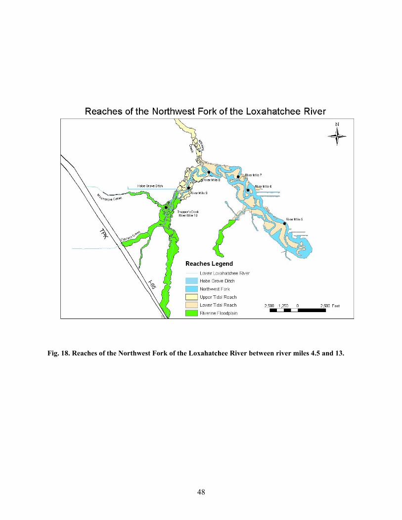
Fig. 18. Reaches of the Northwest Fork of the Loxahatchee River between river miles 4.5 and 13.
48
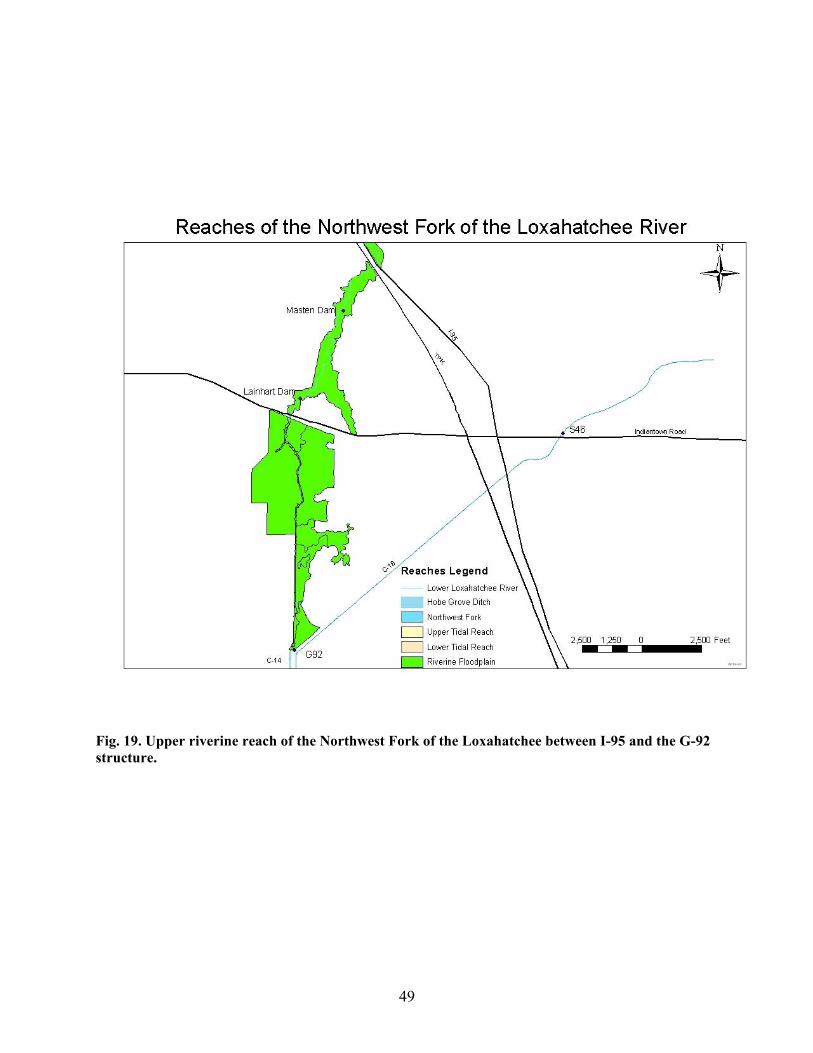
ig. 19. Upper riverine reach of the Northwest Fork of the Loxahatchee between I-95 and the G-92 structure.
F
49
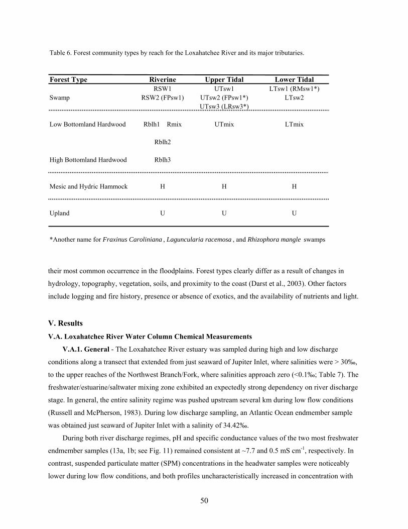
Table 6. Forest community types by reach for the Loxahatchee River and its major tributaries.
Forest Type Riverine Upper Tidal Lower TidalRSW1 UTsw1 LTsw1 (RMsw1*)
Swamp RSW2 (FPsw1) UTsw2 (FPsw1*) LTsw2UTsw3 (LRsw3*)
Low Bottomland Hardwood Rblh1 Rmix UTmix LTmix
Rblh2
High Bottomland Hardwood Rblh3
Mesic and Hydric Hammock H H H
Upland U U U
*Another name for Fraxinus Caroliniana , Laguncularia racemosa , and Rhizophora mangle swamps
their most common occurrence in the floodplains. Forest types clearly differ as a result of changes in
hydrology, topography, vegetation, soils, and proximity to the coast (Darst et al., 2003). Other factors
include logging and fire history, presence or absence of exotics, and the availability of nutrients and light.
V. Results V.A. Loxahatchee River Water Column Chemical Measurements
V.A.1. General - The Loxahatchee River estuary was sampled during high and low discharge
conditions along a transect that extended from just seaward of Jupiter Inlet, where salinities were > 30‰,
to the upper reaches of the Northwest Branch/Fork, where salinities approach zero (<0.1‰; Table 7). The
freshwater/estuarine/saltwater mixing zone exhibited an expectedly strong dependency on river discharge
stage. In general, the entire salinity regime was pushed upstream several km during low flow conditions
(Russell and McPherson, 1983). During low discharge sampling, an Atlantic Ocean endmember sample
was obtained just seaward of Jupiter Inlet with a salinity of 34.42‰.
During both river discharge regimes, pH and specific conductance values of the two most freshwater
endmember samples (13a, 1b; see Fig. 11) remained consistent at ~7.7 and 0.5 mS cm-1, respectively. In
contrast, suspended particulate matter (SPM) concentrations in the headwater samples were noticeably
lower during low flow conditions, and both profiles uncharacteristically increased in concentration with
50
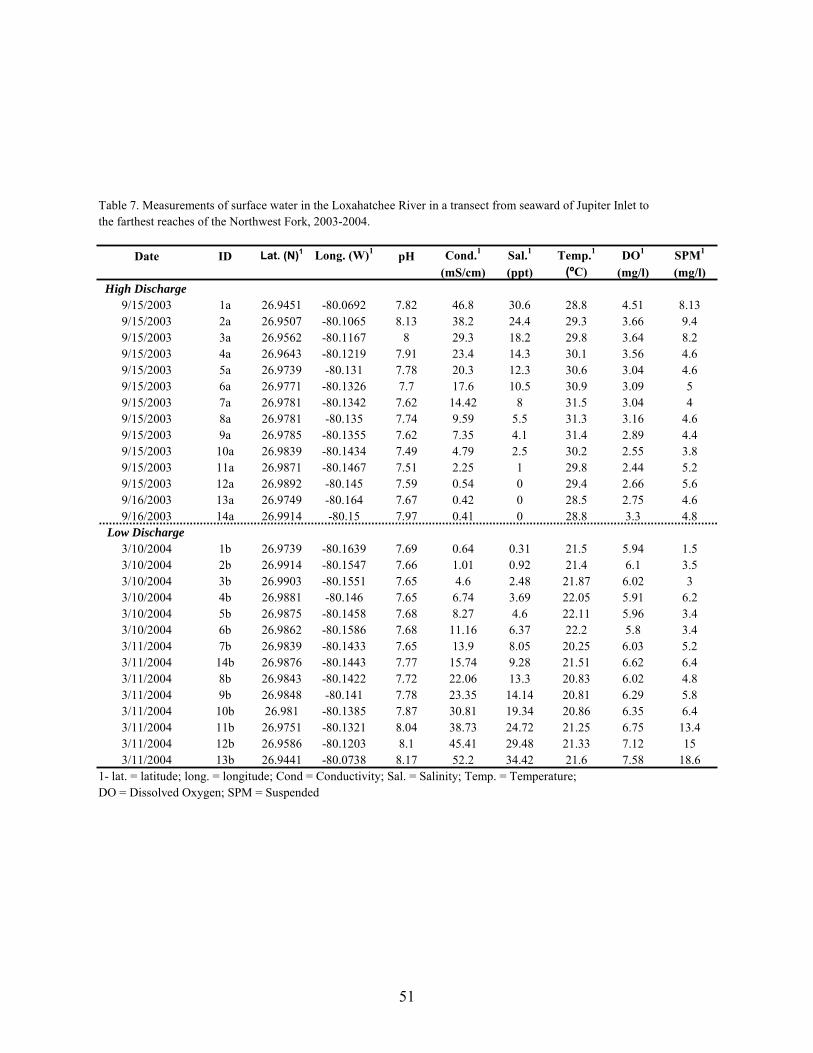
Table 7. Measurements of surface water in the Loxahatchee River in a transect from seaward of Jupiter Inlet to the farthest reaches of the Northwest Fork, 2003-2004.
Date ID Lat. (N)1 Long. (W)1 pH Cond.1 Sal.1 Temp.1 DO1 SPM1
(mS/cm) (ppt) (ºC) (mg/l) (mg/l)High Discharge
9/15/2003 1a 26.9451 -80.0692 7.82 46.8 30.6 28.8 4.51 8.139/15/2003 2a 26.9507 -80.1065 8.13 38.2 24.4 29.3 3.66 9.49/15/2003 3a 26.9562 -80.1167 8 29.3 18.2 29.8 3.64 8.29/15/2003 4a 26.9643 -80.1219 7.91 23.4 14.3 30.1 3.56 4.69/15/2003 5a 26.9739 -80.131 7.78 20.3 12.3 30.6 3.04 4.69/15/2003 6a 26.9771 -80.1326 7.7 17.6 10.5 30.9 3.09 59/15/2003 7a 26.9781 -80.1342 7.62 14.42 8 31.5 3.04 49/15/2003 8a 26.9781 -80.135 7.74 9.59 5.5 31.3 3.16 4.69/15/2003 9a 26.9785 -80.1355 7.62 7.35 4.1 31.4 2.89 4.49/15/2003 10a 26.9839 -80.1434 7.49 4.79 2.5 30.2 2.55 3.89/15/2003 11a 26.9871 -80.1467 7.51 2.25 1 29.8 2.44 5.29/15/2003 12a 26.9892 -80.145 7.59 0.54 0 29.4 2.66 5.69/16/2003 13a 26.9749 -80.164 7.67 0.42 0 28.5 2.75 4.69/16/2003 14a 26.9914 -80.15 7.97 0.41 0 28.8 3.3 4.8
Low Discharge3/10/2004 1b 26.9739 -80.1639 7.69 0.64 0.31 21.5 5.94 1.53/10/2004 2b 26.9914 -80.1547 7.66 1.01 0.92 21.4 6.1 3.53/10/2004 3b 26.9903 -80.1551 7.65 4.6 2.48 21.87 6.02 33/10/2004 4b 26.9881 -80.146 7.65 6.74 3.69 22.05 5.91 6.23/10/2004 5b 26.9875 -80.1458 7.68 8.27 4.6 22.11 5.96 3.43/10/2004 6b 26.9862 -80.1586 7.68 11.16 6.37 22.2 5.8 3.43/11/2004 7b 26.9839 -80.1433 7.65 13.9 8.05 20.25 6.03 5.23/11/2004 14b 26.9876 -80.1443 7.77 15.74 9.28 21.51 6.62 6.43/11/2004 8b 26.9843 -80.1422 7.72 22.06 13.3 20.83 6.02 4.83/11/2004 9b 26.9848 -80.141 7.78 23.35 14.14 20.81 6.29 5.83/11/2004 10b 26.981 -80.1385 7.87 30.81 19.34 20.86 6.35 6.43/11/2004 11b 26.9751 -80.1321 8.04 38.73 24.72 21.25 6.75 13.43/11/2004 12b 26.9586 -80.1203 8.1 45.41 29.48 21.33 7.12 153/11/2004 13b 26.9441 -80.0738 8.17 52.2 34.42 21.6 7.58 18.6
1- lat. = latitude; long. = longitude; Cond = Conductivity; Sal. = Salinity; Temp. = Temperature;DO = Dissolved Oxygen; SPM = Suspended
51
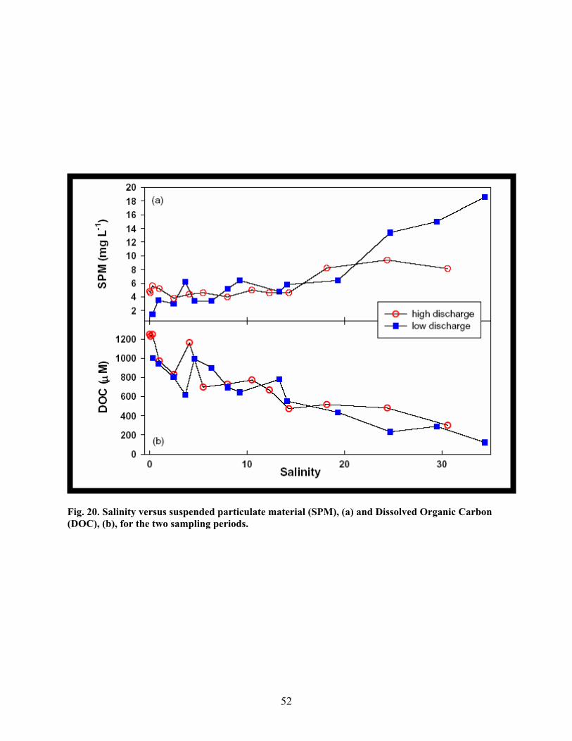
te material (SPM), (a) and Dissolved Organic Carbon OC), (b), for the two sampling periods.
Fig. 20. Salinity versus suspended particula(D
52
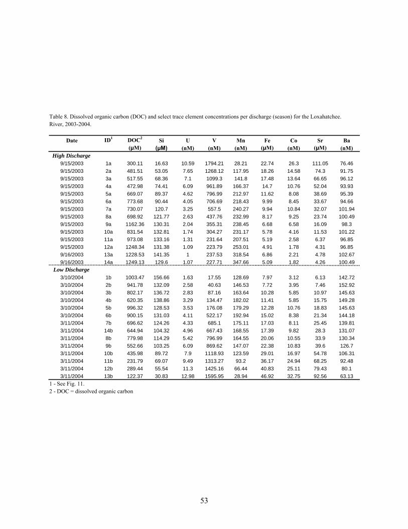
Table 8. Dissolved organic carbon (DOC) and select trace element concentrations per discharge (season) for the Loxahatchee.River, 2003-2004.
Date ID1 DOC2 Si U V Mn Fe Co Sr Ba(µM) (µM) (nM) (nM) (nM) (µM) (nM) (µM) (nM)
High Discharge9/15/2003 1a 300.11 16.63 10.59 1794.21 28.21 22.74 26.3 111.05 76.469/15/2003 2a 481.51 53.05 7.65 1268.12 117.95 18.26 14.58 74.3 91.759/15/2003 3a 517.55 68.36 7.1 1099.3 141.8 17.48 13.64 66.65 96.129/15/2003 4a 472.98 74.41 6.09 961.89 166.37 14.7 10.76 52.04 93.939/15/2003 5a 669.07 89.37 4.62 796.99 212.97 11.62 8.08 38.69 95.399/15/2003 6a 773.68 90.44 4.05 706.69 218.43 9.99 8.45 33.67 94.669/15/2003 7a 730.07 120.7 3.25 557.5 240.27 9.94 10.84 32.07 101.949/15/2003 8a 698.92 121.77 2.63 437.76 232.99 8.17 9.25 23.74 100.499/15/2003 9a 1162.36 130.31 2.04 355.31 238.45 6.68 6.58 16.09 98.39/15/2003 10a 831.54 132.81 1.74 304.27 231.17 5.78 4.16 11.53 101.229/15/2003 11a 973.08 133.16 1.31 231.64 207.51 5.19 2.58 6.37 96.859/15/2003 12a 1248.34 131.38 1.09 223.79 253.01 4.91 1.78 4.31 96.859/16/2003 13a 1228.53 141.35 1 237.53 318.54 6.86 2.21 4.78 102.679/16/2003 14a 1249.13 129.6 1.07 227.71 347.66 5.09 1.82 4.26 100.49
Low Discharge3/10/2004 1b 1003.47 156.66 1.63 17.55 128.69 7.97 3.12 6.13 142.723/10/2004 2b 941.78 132.09 2.58 40.63 146.53 7.72 3.95 7.46 152.923/10/2004 3b 802.17 136.72 2.83 87.16 163.64 10.28 5.85 10.97 145.633/10/2004 4b 620.35 138.86 3.29 134.47 182.02 11.41 5.85 15.75 149.283/10/2004 5b 996.32 128.53 3.53 176.08 179.29 12.28 10.76 18.83 145.633/10/2004 6b 900.15 131.03 4.11 522.17 192.94 15.02 8.38 21.34 144.183/11/2004 7b 696.62 124.26 4.33 685.1 175.11 17.03 8.11 25.45 139.813/11/2004 14b 644.94 104.32 4.96 667.43 168.55 17.39 9.82 28.3 131.073/11/2004 8b 779.98 114.29 5.42 796.99 164.55 20.06 10.55 33.9 130.343/11/2004 9b 552.66 103.25 6.09 869.62 147.07 22.38 10.83 39.6 126.73/11/2004 10b 435.98 89.72 7.9 1118.93 123.59 29.01 16.97 54.78 106.313/11/2004 11b 231.79 69.07 9.49 1313.27 93.2 36.17 24.94 68.25 92.483/11/2004 12b 289.44 55.54 11.3 1425.16 66.44 40.83 25.11 79.43 80.13/11/2004 13b 122.37 30.83 12.98 1595.95 28.94 46.92 32.75 92.56 63.13
1 - See Fig. 11.2 - DOC = dissolved organic carbon
53
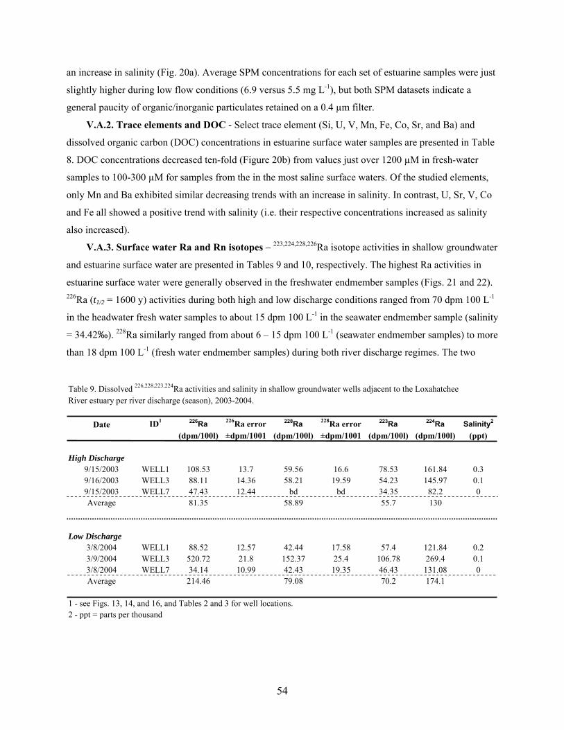
an increase in salinity (Fig. 20a). Average SPM concentrations for each set of estuarine samples were just
slightly higher during low flow conditions (6.9 versus 5.5 mg L-1), but both SPM datasets indicate a
general paucity of organic/inorganic particulates retained on a 0.4 µm filter.
V.A.2. Trace elements and DOC - Select trace element (Si, U, V, Mn, Fe, Co, Sr, and Ba) and
dissolved organic carbon (DOC) concentrations in estuarine surface water samples are presented in Table
8. DOC concentrations decreased ten-fold (Figure 20b) from values just over 1200 µM in fresh-water
samples to 100-300 µM for samples from the in the most saline surface waters. Of the studied elements,
only Mn and Ba exhibited similar decreasing trends with an increase in salinity. In contrast, U, Sr, V, Co
and Fe all showed a positive trend with salinity (i.e. their respective concentrations increased as salinity
also increased).
V.A.3. Surface water Ra and Rn isotopes – 223,224,228,226Ra isotope activities in shallow groundwater
and estuarine surface water are presented in Tables 9 and 10, respectively. The highest Ra activities in
estuarine surface water were generally observed in the freshwater endmember samples (Figs. 21 and 22). 226Ra (t1/2 = 1600 y) activities during both high and low discharge conditions ranged from 70 dpm 100 L-1
in the headwater fresh water samples to about 15 dpm 100 L-1 in the seawater endmember sample (salinity
= 34.42‰). 228Ra similarly ranged from about 6 – 15 dpm 100 L-1 (seawater endmember samples) to more
than 18 dpm 100 L-1 (fresh water endmember samples) during both river discharge regimes. The two
Table 9. Dissolved 226,228,223,224Ra activities and salinity in shallow groundwater wells adjacent to the Loxahatchee River estuary per river discharge (season), 2003-2004.
Date ID1 226Ra 226Ra error 228Ra 228Ra error 223Ra 224Ra Salinity2
(dpm/100l) ±dpm/1001 (dpm/100l) ±dpm/1001 (dpm/100l) (dpm/100l) (ppt)
High Discharge9/15/2003 WELL1 108.53 13.7 59.56 16.6 78.53 161.84 0.39/16/2003 WELL3 88.11 14.36 58.21 19.59 54.23 145.97 0.19/15/2003 WELL7 47.43 12.44 bd bd 34.35 82.2 0Average 81.35 58.89 55.7 130
Low Discharge3/8/2004 WELL1 88.52 12.57 42.44 17.58 57.4 121.84 0.23/9/2004 WELL3 520.72 21.8 152.37 25.4 106.78 269.4 0.13/8/2004 WELL7 34.14 10.99 42.43 19.35 46.43 131.08 0Average 214.46 79.08 70.2 174.1
1 - see Figs. 13, 14, and 16, and Tables 2 and 3 for well locations.2 - ppt = parts per thousand
54
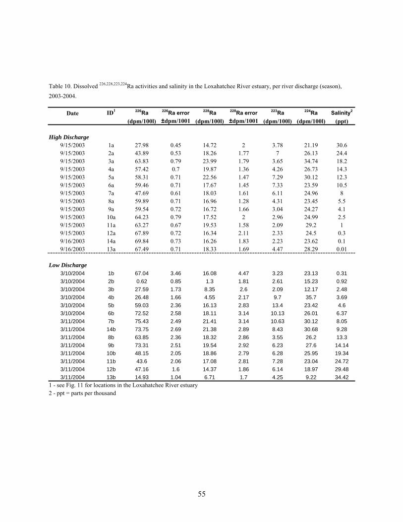
Table 10. Dissolved 226,228,223,224Ra activities and salinity in the Loxahatchee River estuary, per river discharge (season),2003-2004.
Date ID1 226Ra 226Ra error 228Ra 228Ra error 223Ra 224Ra Salinity2
(dpm/100l) ±dpm/1001 (dpm/100l) ±dpm/1001 (dpm/100l) (dpm/100l) (ppt)
High Discharge9/15/2003 1a 27.98 0.45 14.72 2 3.78 21.19 30.69/15/2003 2a 43.89 0.53 18.26 1.77 7 26.13 24.49/15/2003 3a 63.83 0.79 23.99 1.79 3.65 34.74 18.29/15/2003 4a 57.42 0.7 19.87 1.36 4.26 26.73 14.39/15/2003 5a 58.31 0.71 22.56 1.47 7.29 30.12 12.39/15/2003 6a 59.46 0.71 17.67 1.45 7.33 23.59 10.59/15/2003 7a 47.69 0.61 18.03 1.61 6.11 24.96 89/15/2003 8a 59.89 0.71 16.96 1.28 4.31 23.45 5.59/15/2003 9a 59.54 0.72 16.72 1.66 3.04 24.27 4.19/15/2003 10a 64.23 0.79 17.52 2 2.96 24.99 2.59/15/2003 11a 63.27 0.67 19.53 1.58 2.09 29.2 19/15/2003 12a 67.89 0.72 16.34 2.11 2.33 24.5 0.39/16/2003 14a 69.84 0.73 16.26 1.83 2.23 23.62 0.19/16/2003 13a 67.49 0.71 18.33 1.69 4.47 28.29 0.01
Low Discharge3/10/2004 1b 67.04 3.46 16.08 4.47 3.23 23.13 0.313/10/2004 2b 0.62 0.85 1.3 1.81 2.61 15.23 0.923/10/2004 3b 27.59 1.73 8.35 2.6 2.09 12.17 2.483/10/2004 4b 26.48 1.66 4.55 2.17 9.7 35.7 3.693/10/2004 5b 59.03 2.36 16.13 2.83 13.4 23.42 4.63/10/2004 6b 72.52 2.58 18.11 3.14 10.13 26.01 6.373/11/2004 7b 75.43 2.49 21.41 3.14 10.63 30.12 8.053/11/2004 14b 73.75 2.69 21.38 2.89 8.43 30.68 9.283/11/2004 8b 63.85 2.36 18.32 2.86 3.55 26.2 13.33/11/2004 9b 73.31 2.51 19.54 2.92 6.23 27.6 14.143/11/2004 10b 48.15 2.05 18.86 2.79 6.28 25.95 19.343/11/2004 11b 43.6 2.06 17.08 2.81 7.28 23.04 24.723/11/2004 12b 47.16 1.6 14.37 1.86 6.14 18.97 29.483/11/2004 13b 14.93 1.04 6.71 1.7 4.25 9.22 34.42
1 - see Fig. 11 for locations in the Loxahatchee River estuary2 - ppt = parts per thousand
55
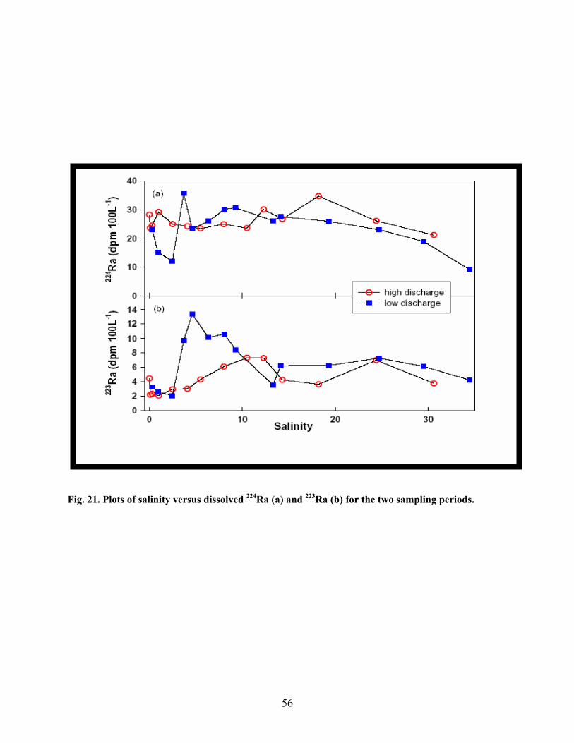
Fig. 21. Plots of salinity versus dissolved 224Ra (a) and 223Ra (b) for the two sampling periods.
56
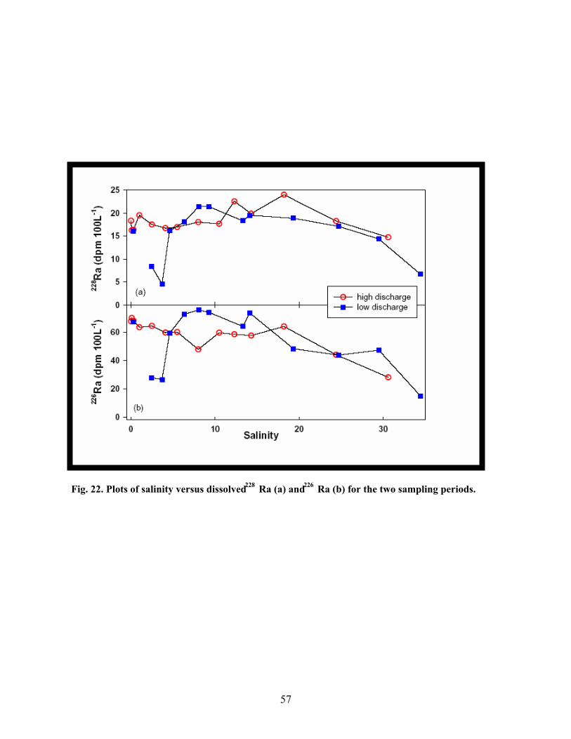
Fig. 22. Plots of salinity versus dissolved Ra (a) and Ra (b) for the two sampling periods.
228 226
57
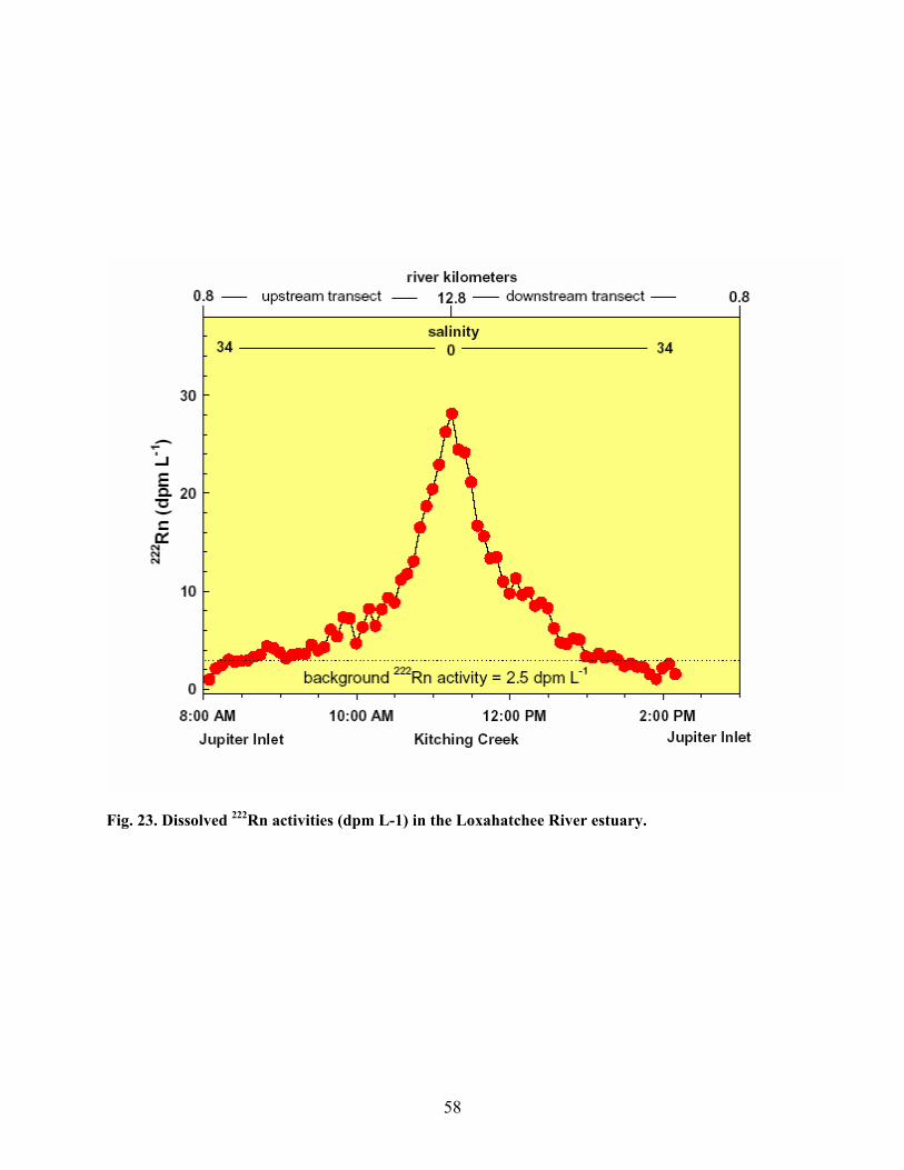
Fig. 23. Dissolved 222Rn activities (dpm L-1) in the Loxahatchee River estuary.
58
short-lived Ra isotopes, 223Ra and 224Ra, ranged in activity from generally < 14 dpm 100 L-1 to 10 – 35
dpm 100L-1, respectively. There is no obvious trend between 223,224Ra and salinity. Excluding the thermal
spring-derived discharge off west-central Florida (Fanning et al., 1981), and the phosphate-enhanced Ra
isotopes observed in Tampa Bay, such Ra activities are typicalfor Florida coastal waters and estuaries
(Burnett et al., 1990; Swarzenski et al., 2001; Swarzenski et al., 2004; Cable et al., 2004).
222Rn activities were measured almost real-time from the seaward endmember close to the Jupiter
Inlet (salinity ~ 34‰) upstream to the confluence of Kitching Creek and the Loxahatchee River, where
salinities approach zero. During this Rn survey, activities were inversely related to salinity (Fig. 23), and
ranged from a background value of ~2.5 dpm L-1 at Jupiter Inlet to more than 28 dpm L-1 at Kitching
Creek.
V.B. Loxahatchee River Floodplain Water Quality Measurements
V.B.1. General - Results of chemical analyses of surface water, porewater, and well water samples
from the Loxahatchee River floodplain sites (transect sites) are presented in tabular form in Appendix A
for both the wet season (September 2003) and dry season (March 2004) sampling. Selected parameters for
surface water and porewater for all sites sampled along transects 1, 3, 6, 7, and 9 for both the wet season
and dry season are plotted versus depth and along the transects in the figures in Appendix B.
V.B.2. pH, alkalinity, and redox – Values for pH at all sites are tabulated in Tables 1 and 3, in
Appendix A, representing the wet and dry season sampling, respectively. Results are plotted in Appendix
B, Figs. 1A-1E. Surface water and porewater pH values ranged from 5.74 to 7.90, but with most samples
having pH values in the range of 6.5-7.8 (circumneutral pH). No major differences in pH were noted
among the different transects, and dry season pH values were generally similar to wet season values at
most sites. Upland wells on Transects 7 and 9 had much more acidic pH values of around 5. These wells
also tended to have low ionic strength. At most sites, pH values tended to decrease with increasing depth
in the sediment, reflecting production of protolytic chemical species (e.g organic acids) during
sedimentary decomposition of organic matter. Along transect 1, a large decrease in pH was seen at site 3
below 5 cm. This may reflect the influence of more acidic groundwater at this most upland site.
Values for titration alkalinity are presented in Appendix A Tables 1 and 3 for the wet and dry
seasons, respectively. Alkalinity values are plotted in Appendix B, Figs. 2A-2E. Alkalinities ranged from
1 to 23 meq/L, but with most samples in the 2 to 5 meq/L range. These are relatively low alkalinities for
porewater. Typically, alkalinities are higher in pore water than surface water, and increase with depth in
pore water due to accumulation of dissolved CO2 from microbial degradation of organic matter in
sediments. The reason(s) for the relatively low alkalinities in the Loxahatchee River floodplain is unclear.
One hypothesis is that tidal effects or upwelling groundwater continually strip dissolved chemical species
59
from pore water. No pattern was observed in the downcore profiles of alkalinity, with some sites
exhibiting increasing alkalinity with depth, some sites showing decreasing alkalinity with depth, and
some sites showing no pattern. Similarly, no consistent pattern was observed in alkalinity between the wet
and dry seasons. Some sites showed slightly higher wet season alkalinities, some showed slightly higher
dry season alkalinities, and some sites showed no difference. Wells had variable alkalinities, but the two
lowest alkalinities observed were from upland wells along Transects 7 and 9. These wells also had low
pH and ionic strength.
Redox values for all sites are presented in Appendix A Tables 1 and 3, for the wet season and dry
season, respectively. Results are plotted in Appendix B Figs. 3A-3E. Redox values range from 219
(highly oxidizing) to -260 mv (highly reducing) in surface and porewater, although most samples had
redox values of 100 to -150 mv. Most surface water redox values were positive, reflecting oxidizing
conditions. Some surface waters, especially from wet season sites along transects 1 and 3, had slightly
negative redox values, suggesting reducing conditions. This could reflect stagnant water conditions, as
well as high levels of dissolved humic substances in the surface water, which can also influence redox
measurements. The most negative (reducing) redox values in porewater were observed along transect 9,
due to the high levels of sulfide in the brackish waters on this transect. Transect 1 had much lower (more
reducing) porewater redox values in the wet season than in the dry season. This is due to the generally dry
(oxidizing) conditions of the sediments during the dry season. Changes in redox values with depth varied
along the different transects. Redox values along transects 1 and 3 initially decreased with depth over the
upper 10 cm, and then increased below this. Redox values at sites on transect 6 showed slight increases
with depth over the upper 15 cm, and then decreased sharply with depth below 15 cm. Redox values
along transect 7 showed little change or a slight decrease with depth, and redox values along transect 9
sharply decreased with depth, especially during the dry season. Wells had variable redox values, but with
the majority having negative values (reducing conditions). More wells had positive (oxidizing) redox
values in the dry season compared to the wet season.
V.B.3. Conductivity, salinity, total dissolved solids – Values for conductivity, salinity, and total
dissolved solids (TDS) are presented in Appendix A Tables 1 (wet season) and 3 (dry season). Results for
conductivity are plotted in Appendix B, Figs. 4A-4E. Plots of salinity and TDS are not included in
Appendix B, but these closely parallel the conductivity plots (from which they are derived). Overall,
conductivity, salinity, and TDS were highest at transect 9 (most downstream transect), and lowest at
transects 1 and 3. At most (but not all) sites, higher conductivity, salinity and TDS values were observed
during the dry season, presumably due to evaporative concentration of salts. Sites exhibiting higher wet
season values for conductivity, salinity, and TDS tended to be those farthest from the river, and
potentially more influenced by groundwater.
60
Conductivity values ranged from 400-900 µS along both transects 1 and 3 during the wet season, and
from 148-1788 µS along transect 1 during the dry season (March 2004). Dry season conductivity results
from transect 3 were somewhat limited due to extremely dry conditions, but results available ranged from
127-776 µS. Depth profiles for conductivity along transects 1 and 3 were similar. Conductivity values
were higher in porewater than in surface for all wet season sites along transects 1 and 3. During the dry
season, however, the more upland sites (site 3 along transect 1, and sites 2 and 3 along transect 3) had
higher surface water conductivity compared to porewater. At sites 2 and 3 along transects 1 and 3,
conductivity had a subsurface maximum at about 10-20 cm during the wet season. At site 2 along transect
1, conductivity increased sharply with depth during the dry season sampling, indicating a source of higher
ionic strength water coming in from below the unconsolidated peat zone. At sites 1 and 3 along transect 1,
dry season conductivity had unsystematic depth profiles, possibly reflecting the influence of evaporative
concentration by drying in the surface sediments and input of saltier water from below the surface.
Conductivity values along transect 6 are 3 to 4 times higher than along transects 1 and 3, reflecting
the closer proximity to the Loxahatchee River mouth at Jupiter Inlet. In the wet season conductivity
increased from 400 to 2,300 µS with depth in porewater along transect 6. During the dry season the
increase in conductivity with depth was much less, from 1500-2000 µS due to higher overall conductivity
values in the surface water and near-surface porewater.
Although transect 7 is in relatively close proximity to transect 6, there are significant differences in
many of the chemical parameters between these two transects. Overall, transect 7 more closely resembles
transect 3 than Transect 6 in its surface and pore water geochemistry. Transect 7 has generally lower
conductivity values compared to transect 6, irrespective of tidal level. For example, conductivity reaches
only about 600 µS along transect 7, compared to nearly 2,500 µS at transect 6. Note that transect 7 was
sampled on 2 different days and over different tidal levels (site 1 at high tide, and site 2 at low tide)
during the wet season. The difference in the tidal level is reflected in lower conductivity values at site 2
compared to site 1. Conductivity shows a slight increase with depth at both sites on transect 7.
As expected, transect 9 had the highest conductivity values, up to nearly 8,000 µS in the wet season
and more than 14,000 µS in the dry season. Interestingly, site 2 on this transect (site closest to the river)
had the lowest conductivity and chloride concentrations, and site 1 (the most landward site) had the
highest, during both the wet and dry seasons. This particular transect is on a small peninsula in the river,
and the orientation of the transect on the peninsula combined with salt wedge movement may explain the
saltier water at the most landward site. Conductivity values increased with depth in the porewater during
the wet season. During the dry season conductivity was generally highest in the surface water and showed
little change with depth until below about 50 cm, where values decreased. Dry season results from site 2
(nearest the river) indicated higher conductivity values during high tide compared to low tide.
61
V.B.4. Chloride, fluoride, bromide – Values for chloride, fluoride, and bromide are presented in
Appendix A Tables 1 (wet season) and 3 (dry season). Results for chloride are plotted in Appendix B,
Figs. 5A-5E. Plots of fluoride and bromide are not included in the Appendix, but these closely parallel the
chloride plots. Chloride, fluoride, and bromide values are generally lowest at the upriver transects (1 and
3), and highest along transect 9 (most marine site), as expected.
Along transect 1, chloride concentrations range from 19-36 mg/L during the wet season, and 28-151
mg/L in the dry season, in surface and porewater. Dry season chloride concentrations are generally higher
at sites 1 and 2, but wet season chloride concentrations are higher at site 3 (most upland site). Site 3
chloride concentrations show little change with depth during the dry season, but an increase with depth
and maximum at 20 cm depth during the wet season. Site 2 chloride concentrations showed a subsurface
maximum at about 10-20cm, that was much more pronounced during the dry season. At site 1 (nearest the
river) chloride concentration increased with depth during the wet season, but decreased with depth during
the dry season.
Chloride concentrations along transect 3 were similar to those along transect 1, and ranged from 17-
105 mg/L during the wet season, and from 14-267 mg/L during the dry season. Chloride concentrations
were the same to slightly higher overall during the dry season at all sites along transect 3.
Along transect 6, chloride concentrations ranged from 44-612 mg/L during the wet season, and 223-
563 mg/L during the dry season. Concentrations at sites 1 and 2 were similar. At site 1 (near river),
chloride concentrations were generally higher during the dry season, and chloride concentrations
increased with depth during both the wet and dry seasons. At site 2, chloride concentrations increased
with depth during the wet season, but a more complex depth profile was observed during the dry season.
Transect 7 chloride concentrations ranged from 21-115 mg/L during the wet season, and 69-200
mg/L during the dry season. Overall concentrations were slightly higher at site 1 (upland site). Chloride
concentrations showed little change with depth, except for a maximum at about 10 cm in the site 1 dry
season data. As with conductivity, transect 7 results for chloride more closely resembled those for
transects 1 and 3 than the nearby transect 6.
Transect 9 had the highest chloride concentrations, ranging from 279-6773 mg/L in the wet season,
and 1414-7720 mg/L in the dry season. Dry season chloride concentrations were generally lower than wet
season concentrations at all sites. As with conductivity, the highest chloride concentrations were observed
at site 1 (most upland site). Transect 9 is on a small peninsula in the river, as previously mentioned, and
the orientation of the transect on the peninsula combined with salt wedge movement may explain the
higher chloride contents at the most landward site. Chloride concentrations at most sites along transect 9
increased with depth to a subsurface maximum, during both the wet and dry seasons. These subsurface
62
maxima are typically at depths of about 10-20 cm, except for the wet season results from site 1, where the
maximum is at 40 cm.
V.B.5. Sulfate and sulfide – Concentrations of sulfate and sulfide are tabulated in Appendix A
Tables 1 (wet season) and 3 (dry season), and plotted in Appendix B, Figs. 6A-6E.(sulfate) and 7A-7E
(sulfide). Overall sulfate and sulfide concentrations were highest at transect 9, and lowest at transects 1
and 3.
Along transect 1, sulfate concentrations ranged from <1-47 mg/L in the wet season, and from 1.6-
209 mg/L in the dry season. Sulfate concentrations were somewhat higher at the river site (site 1)
compared to the more upland sites. Sulfate concentrations were slightly or moderately higher during the
dry season, with the dry season-wet season difference being least at the most upland site. Changes in
sulfate concentration with depth were complex, but for most cores involved an initial decrease in
concentration from the surface water into the pore water, followed by an increase toward the bottom of
the profile. This overall trend is consistent with microbial sulfate reduction occurring in the near surface
sediment zone, and a source of sulfate at depth. Well water from transect 1 (site 1) had significantly
higher sulfate concentration in the wet season.
Sulfide concentrations in the surface and porewater along transect 1 were low, but measurable,
ranging from 1-32 µg/L during the wet season, and <0.1-184 µg/L during the dry season. The presence of
sulfide indicates that microbial sulfate reduction is occurring in these sediments, but with sulfide buildup
limited by sulfate availability, daily tidal pumping, and precipitation of insoluble metal sulfides. Sulfide
concentrations were similar during the wet and dry seasons at transect 1 sites 1 and 2, but were
significantly higher during the dry season at transect 1 site 3. Sulfide profiles generally exhibited a mid-
depth maximum, indicating the zone where maximal microbial sulfate reducing activity is occurring, and
where sulfide advection/diffusion out of the porewater is limited. Well water had sulfide concentrations of
52 µg/L in the wet season, and 26 µg/L in the dry season.
Transect 3 had sulfate concentrations ranging from 1-63 mg/L in the wet season, and 1-44 mg/L in
the dry season, similar to values observed along transect 1. Transect 3 also had somewhat lower sulfate
concentrations at site 3 (upland site), similar to what was observed at transect 1. In contrast to transect 1,
however, dry season sulfate concentrations along transect 3 were either about the same, or higher
compared to the wet season. As with transect 1, sulfate concentrations along transect 3 commonly showed
an initial decrease with depth, followed by an increase toward the bottom of the profile. Again, this is
consistent with microbial sulfate reduction in the near surface zone, and a source of sulfate at depth.
Sulfide concentrations along Transect 3 were similar to those observed along transect 1. Wet season
sulfide concentrations ranged from 2-37 µg/L, and dry season concentrations from <0.1-165 µg/L. Higher
overall dry season sulfide concentrations along transect 3 reflect overall higher dry season sulfate
63

concentrations. Downcore sulfide profiles showed generally increasing concentrations with depth to the
bottom of the profile. This reflects the high sulfate concentrations found at the base of many of the
profiles along transect 3. Well water from near transect 3 site 1 had much higher dry season sulfide
concentrations (204 µg/L) compared to the wet season (11.8 µg/L), although higher sulfate concentrations
were observed in the well water during the wet season. This result is somewhat surprising, since one
normally anticipates higher rates of microbial sulfate reduction with higher levels of sulfide and lower
sulfate during the warmer wet season.
Transect 6 had sulfate concentrations slightly higher than those at transects 1 and 3. Sulfate
concentrations along transect 6 ranged from <1-139 mg/L in the wet season, and 21-84 mg/L in the dry
season. Sulfate concentrations were approximately the same at both sites along the transect. Dry season
sulfate concentrations were higher than wet season concentrations, except at the base of each profile. The
wet season profiles at both sites showed a sharp increase in sulfate concentrations at the bottom of the
profile, suggesting a source of sulfate at depth. This increase in sulfate concentrations at the base of the
profile was not observed in the dry season. The wet season depth profiles for sulfate were similar to those
observed at transects 1 and 3: an initial decrease in sulfate concentration (microbial sulfate reduction),
followed by an increase in sulfate near the base of the profile suggesting a sulfate source at depth. The dry
season sulfate profiles along transect 6 showed only a slow decrease in sulfate concentration with depth.
Sulfide concentrations along transect 6 ranged from 1-1840 µg/L in the wet season, and <1-2557
µg/L in the dry season. The major characteristic of the sulfide data along transect 6 is the large increase in
concentration below 20 cm, especially at the more upland site (site 2). This indicates that microbial
sulfate reduction and accumulation of sulfide in porewater is occurring below 20 cm at this transect.
Normally, maximum microbial sulfate reduction activity is located in the near surface zone. It may be that
microbial sulfate reduction is high near the surface, but that sulfide is being continuously removed by
advective flux, such as tidal action. The sulfate data also indicates a source of sulfate at depth at these
sites, and this likely stimulates microbial sulfate reduction and sulfide accumulation at depth along this
transect.
Transect 7 had overall sulfate concentrations more similar to transects 1 and 3 than to nearby transect
6, which is consistent with the chloride and conductivity results discussed earlier. Sulfate concentrations
ranged from <1-19 mg/L during the wet season, and 1-105 mg/L in the dry season. Overall higher sulfate
concentrations were observed during the dry season along transect 7. During the wet season, sulfate
concentrations generally showed a decrease with depth, followed by an increase near the base of the
profile. Again, this is consistent with microbial sulfate reduction in the near surface zone, and a source of
sulfate at depth. The dry season data, however, showed an initial increase in sulfate with depth to a
subsurface maximum, followed by a decrease in sulfate concentration to the bottom of the profile. This
64
may reflect decreased freshwater flow during the dry season, and increased sulfate in near surface
porewater from tidal action. The decrease in sulfate concentration toward the base of the profile may
reflect the microbial sulfate reduction zone during the dry season along this transect. Well water from the
river site (site 2) had much higher sulfate concentrations compared to the upland site (site 1). No
differences in sulfate concentration between the wet and dry seasons were observed at either well along
transect 7.
Sulfide concentrations along transect 7 ranged from 1-1458 µg/L during the wet season, and <1-710
µg/L during the dry season. As at transect 6, the most interesting characteristic of the sulfide data was the
dramatic increase in concentration below 20 cm at both sites, but especially at the more upland site (site
1). Again, this feature of the sulfide data may reflect advective tidal flux of sulfide from porewater in the
near surface zone, and a source of sulfate at depth that stimulates microbial sulfate reduction and
accumulation of sulfide. Sulfide in the well water was somewhat higher at the upland site (site 1). This is
in contrast to the sulfate data, which was much higher at the river site (site 2). Sulfide concentrations
were somewhat higher at both wells sampled along transect 7 during the dry season.
Sulfate concentrations along transect 9 ranged from 16-1259 mg/L during the wet season, and 284-
1067 mg/L during the dry season. As with chloride and conductivity, the overall highest sulfate
concentrations were observed at the most upland site (site 1) along transect 9. Dry season sulfate
concentrations were generally significantly higher than wet season sulfate concentrations, reflecting
decreased freshwater flow (increased marine influence) during the dry season. Sulfate had differing wet
season-dry season profiles. Wet season profiles had lower overall sulfate concentrations, and showed a
general pattern of initial decreasing sulfate concentration over the upper 2-10 cm, followed by increasing
sulfate concentration to the bottom of the profile. During the dry season, sulfate depth profiles showed
either a gradual decrease in sulfate with depth (site 3), or an initial increase to a subsurface maximum at
about 20 cm, followed by a decrease, and then another increase to the base of the profile (sites 1 and 2).
The upland well along transect 9 had >10 fold lower sulfate concentrations than the river well (near site
2). The upland well had higher wet season sulfate concentrations, while the river well had higher dry
season sulfate concentrations.
Sulfide concentrations along transect 9 ranged from 2-179 µg/L during the wet season, and <1-3007
µg/L during the dry season. However, sulfide levels were relatively low in the near-surface zone (above
20 cm) at all sites, and were especially low overall during the wet season. As with transects 6 and 7, the
characteristic feature of the sulfide data along transect 9 was the very large increase in concentration
below 20 cm. Again, this type of profile is likely driven by advective tidal flux of sulfide from pore water
in the near-surface zone, and by a source of sulfate at depth along this transect. Although sulfate
concentrations were highest at the most upland site along this transect (site 1), sulfide concentrations were
65
highest at the river site (site 2), and lowest at the upland site (site 1). Higher sulfide concentrations (much
higher at sites 2 and 3) were observed during the dry season; probably reflecting decreased freshwater
flux and greater marine influence during the dry season. Sulfide concentrations in wells were higher at the
river end well, and lower at the upland well, consistent with the sulfate data.
V.B.6. Nitrate, ammonium, and phosphate – Concentrations of nutrients (nitrate, ammonium, and
phosphate) are tabulated in Appendix A Tables 2 (wet season) and 4 (dry season), and plotted in
Appendix B, Figs. 8A-8E (nitrate), 9A-9E (ammonium), and 10A-10E (phosphate). In contrast to
parameters such as conductivity, salinity, chloride, and sulfate that are linked to the increasing influence
of saltwater progressing downstream, nutrients do not generally increase from Transect 1 to Transect 9.
Indeed, for phosphate and nitrate, the upstream transects (1 and 3) have the overall highest concentrations.
Also, at most sites wet season nutrient concentrations were significantly higher than dry season
concentrations.
The principal feature of the nutrient (nitrate, ammonium, and phosphate) profiles along transect 1 at
all sites is a subsurface maximum in concentration. The depth of this maximum varies from site to site,
but at each site is at the same depth for nitrate, ammonium, and phosphate. This maximum represents the
zone of primary organic matter decomposition, and recycling of N and P from organic matter deposited in
the sediments. Concentrations of nutrients at all three sites along transect 1 were higher during the wet
season, especially at sites 2 and 3. Phosphorus levels were uniformly high, and in many instances
exceeded the combined nitrate and ammonium concentrations. Thus, primary production along this
transect may be nitrogen limited, although further verification of this is certainly needed. Concentrations
of nutrients in the well from transect 1 (located near site 3) were significantly lower than the maximum
concentrations observed in the porewater during the wet season, but comparable to the dry season
concentrations. There was little difference between wet season and dry season concentrations for
phosphate and ammonium in the well water, but nitrate was significantly higher in the wet season.
Transect 3 had overall lower nitrate concentrations compared to transect 1, especially during the wet
season. Ammonium and phosphate concentrations, however, were generally higher along transect 3
compared to transect 1. Wet season phosphate concentrations were significantly higher than dry season
concentrations along transect 3, as was also observed along transect 1. Overall, wet season concentrations
for nitrate and ammonium were also higher than dry season concentrations, but not in all instances, and
not to the extent seen along transect 1. Depth profiles of nutrient elements along transect 3 also exhibited
generally increasing concentrations from surface water into the porewater, and mid-depth concentration
maxima, as also observed along transect 1. The concentration maxima represent zones of highest
biodegradation of organic N and P in the sediments and production of dissolved nutrient species. As along
transect 1, phosphate concentrations in porewater along transect 3 are elevated relative to ammonium and
66
nitrate concentrations, in many cases exceeding the combined nitrate plus ammonium concentration.
Again, this suggests the possibility that the floodplain vegetation is nitrogen limited. Well water from
transect 3 (well located near site 3) had nutrient concentrations generally lower than wet season porewater
nutrient concentrations, but comparable to dry season porewater nutrient concentrations. Nitrate,
ammonium, and phosphate concentrations in well water from transect 3 were all higher in the wet season.
As with the porewater, well water also had phosphate values that exceeded the total nitrate and
ammonium concentrations.
Overall nitrate concentrations along transect 6 are similar to those observed along transect 3, and
lower than values observed along transect 1. Ammonium and phosphate concentrations are generally
lower than those observed along transects 1 and 3. Wet season concentrations for nitrate, ammonium, and
phosphate were generally much higher than dry season concentrations, as observed along transects 1 and
3. Indeed, along transect 6 dry season porewater concentrations of nutrients were actually less than those
observed in the surface water. Depth profiles, especially during the wet season, exhibited increasing
concentrations of all nutrients from surface water into the porewater building to a subsurface maximum
concentration at about 10 cm for ammonium and phosphate, and 10-20 cm for nitrate.
The two sites along transect 7 have similar nitrate concentrations, but phosphate and ammonium
concentrations during the wet season are much higher at the landward site (site 1). As along transect 6,
dry season concentrations of nutrients are generally lower in porewater than in surface water. As on other
transects, depth profiles for ammonium and phosphate during the wet season along transect 7 exhibit
subsurface maxima. This is especially apparent in the landward (site 1) profile. Well water samples had
higher concentrations of nitrate at the upland well site during the wet season, but much higher
concentrations of phosphate and ammonium at the well near the river. Thus, the well water results are
exactly the reverse of the porewater results, and concentrations of ammonium and phosphate in the well
near the river are considerably higher than those observed in porewater at the river site. Reasons for this
difference are unclear. All well water nutrient concentrations were higher in the wet season.
Nitrate concentrations along transect 9 were generally comparable to those observed along transects
3, 6, and 7, but lower than those from transect 1. Ammonium and phosphate concentrations were
generally comparable to those along transect 7. As elsewhere, nutrient concentrations in porewater along
transect 9 were generally higher during the wet season. Vertical profiles, especially for ammonium and
phosphate showed a sharp increase from surface water into porewater to a subsurface maximum during
the wet season. This was also observed along most other transects. Ammonium and phosphate
concentrations were highest in porewater from the most landward site (site 1). The upland well also had
higher phosphate and ammonium values compared to the river well, exactly the opposite of what was
observed in wells from transect 7. All of the well nutrient data was higher during the wet season, except
67
for phosphate at the river well. Ammonium and phosphate at the upland well had much higher
concentrations during the wet season.
V.B.7. Sodium, potassium, magnesium, and calcium - Concentrations of major cations (sodium,
potassium, magnesium, and calcium) are tabulated in Appendix A Tables 3 (wet season) and 4 (dry
season), and plotted in Appendix B, Figs. 11A-11E (sodium), 12A-12E (potassium), 13A-13E
(magnesium), and 14A-14E (calcium). Overall, sodium, potassium, and magnesium concentrations appear
to be directly linked to degree of saltwater influence, and tend to increase downstream. Calcium
concentrations, however, show no significant changes downstream. Calcium in surface and porewater
may be controlled by diagenetic factors that determine equilibrium concentrations of calcium between the
porewater and the soils/sediments. All four major cations show generally higher concentrations in
porewater along transects 6 and 9 (the most marine sites) during the dry season, reflecting lower
freshwater discharge. No consistent trends in the major cations were observed between the wet and dry
seasons along transects 1, 3, and 7.
Sodium concentrations in surface and porewater range from 2-843 mg/L during the wet season, and
from 0.3-1132 mg/L during the dry season. During the wet season, most sites showed increasing sodium
concentrations from surface water to porewater, and increasing sodium concentrations with depth in the
porewater. During the dry season, however, changes in sodium concentration between surface water and
porewater, and with depth in the porewater were inconsistent. Sodium concentrations were highly
correlated with chloride during the wet season (Fig. 24A), however, this correlation broke down during
the dry season, especially at higher salinities (Fig. 24B). Correlation coefficients (r2 values) between
sodium and chloride were 1.0 during the wet season and 0.86 during the dry season. This suggests that
mixing of salt and fresh water dominates both chloride and sodium concentrations during the wet season,
but other processes may dominate during the dry season. All wells, except the well closest to the river
along transect 9, showed higher wet season concentrations of sodium. Upland wells had generally lower
sodium concentrations than wells nearer the river.
Potassium concentrations in surface and porewater ranged from <1-168 mg/L in the wet season, and
<1-119 mg/L in the dry season. Magnesium concentrations in surface and pore water ranged from <1-470
mg/L in the wet season, and from <1-514 mg/L in the dry season. Potassium and magnesium
concentrations in surface and porewater were generally correlated with sodium concentrations, though
more strongly during the wet season compared to the dry season. Correlation coefficients (r2 values)
between potassium and sodium were 0.98 in the wet season, and 0.86 during the dry season; and between
magnesium and sodium were 0.96 in both the wet and dry season. As with sodium, both potassium and
magnesium concentrations were strongly correlated with chloride concentrations, especially during the
wet season. Changes in potassium and magnesium concentrations from surface water to porewater, and
68
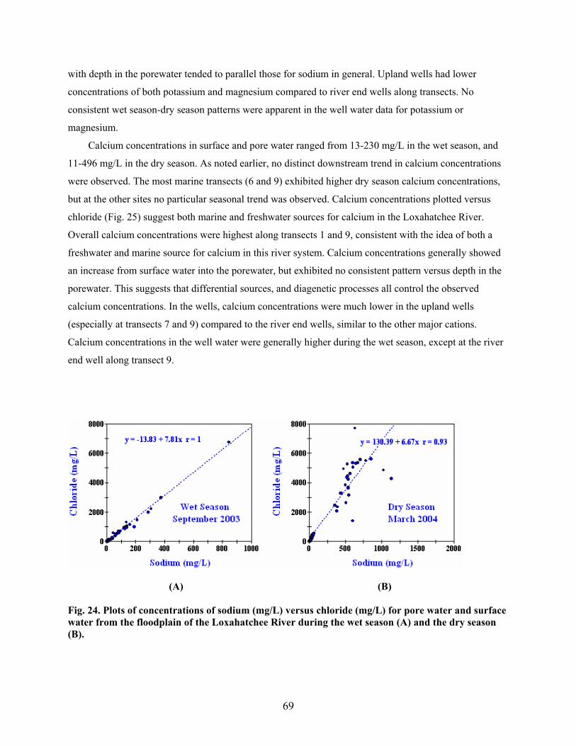
with depth in the porewater tended to parallel those for sodium in general. Upland wells had lower
concentrations of both potassium and magnesium compared to river end wells along transects. No
consistent wet season-dry season patterns were apparent in the well water data for potassium or
magnesium.
Calcium concentrations in surface and pore water ranged from 13-230 mg/L in the wet season, and
11-496 mg/L in the dry season. As noted earlier, no distinct downstream trend in calcium concentrations
were observed. The most marine transects (6 and 9) exhibited higher dry season calcium concentrations,
but at the other sites no particular seasonal trend was observed. Calcium concentrations plotted versus
chloride (Fig. 25) suggest both marine and freshwater sources for calcium in the Loxahatchee River.
Overall calcium concentrations were highest along transects 1 and 9, consistent with the idea of both a
freshwater and marine source for calcium in this river system. Calcium concentrations generally showed
an increase from surface water into the porewater, but exhibited no consistent pattern versus depth in the
porewater. This suggests that differential sources, and diagenetic processes all control the observed
calcium concentrations. In the wells, calcium concentrations were much lower in the upland wells
(especially at transects 7 and 9) compared to the river end wells, similar to the other major cations.
Calcium concentrations in the well water were generally higher during the wet season, except at the river
end well along transect 9.
(A) (B)
Fig. 24. Plots of concentrations of sodium (mg/L) versus chloride (mg/L) for pore water and surface water from the floodplain of the Loxahatchee River during the wet season (A) and the dry season (B).
69
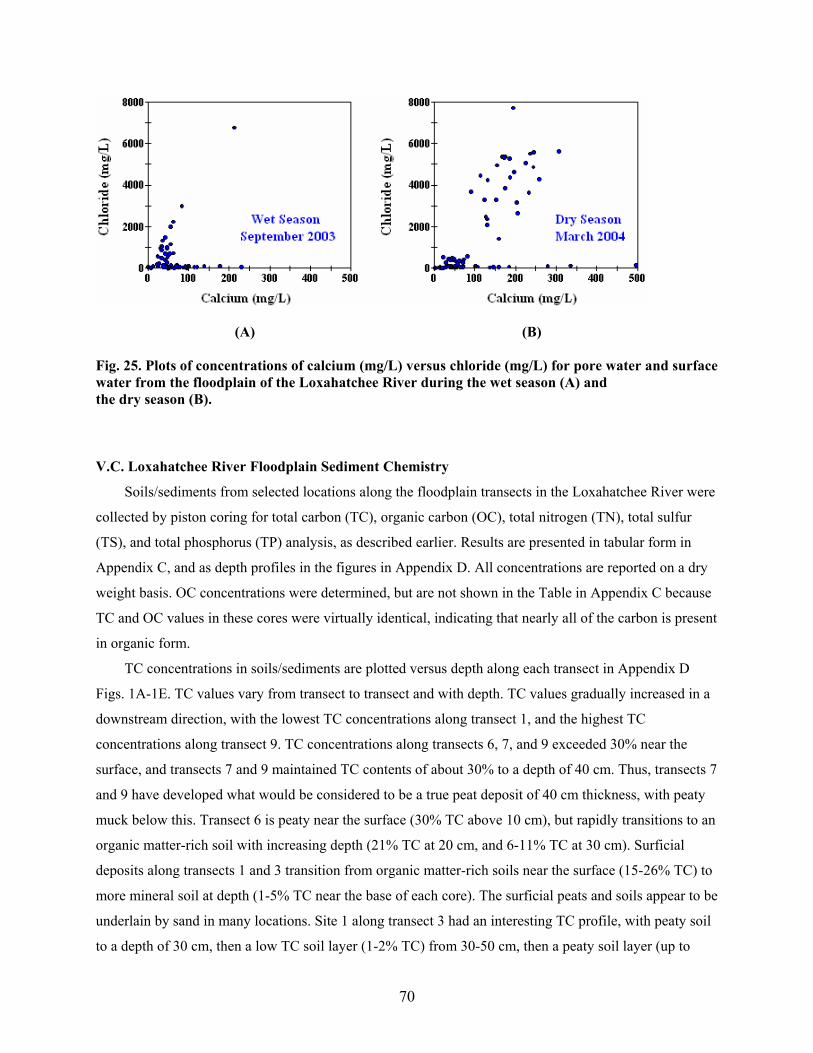
(A) (B)
Fig. 25. Plots of concentrations of calcium (mg/L) versus chloride (mg/L) for pore water and surface water from the floodplain of the Loxahatchee River during the wet season (A) and the dry season (B).
V.C. Loxahatchee River Floodplain Sediment Chemistry
Soils/sediments from selected locations along the floodplain transects in the Loxahatchee River were
collected by piston coring for total carbon (TC), organic carbon (OC), total nitrogen (TN), total sulfur
(TS), and total phosphorus (TP) analysis, as described earlier. Results are presented in tabular form in
Appendix C, and as depth profiles in the figures in Appendix D. All concentrations are reported on a dry
weight basis. OC concentrations were determined, but are not shown in the Table in Appendix C because
TC and OC values in these cores were virtually identical, indicating that nearly all of the carbon is present
in organic form.
TC concentrations in soils/sediments are plotted versus depth along each transect in Appendix D
Figs. 1A-1E. TC values vary from transect to transect and with depth. TC values gradually increased in a
downstream direction, with the lowest TC concentrations along transect 1, and the highest TC
concentrations along transect 9. TC concentrations along transects 6, 7, and 9 exceeded 30% near the
surface, and transects 7 and 9 maintained TC contents of about 30% to a depth of 40 cm. Thus, transects 7
and 9 have developed what would be considered to be a true peat deposit of 40 cm thickness, with peaty
muck below this. Transect 6 is peaty near the surface (30% TC above 10 cm), but rapidly transitions to an
organic matter-rich soil with increasing depth (21% TC at 20 cm, and 6-11% TC at 30 cm). Surficial
deposits along transects 1 and 3 transition from organic matter-rich soils near the surface (15-26% TC) to
more mineral soil at depth (1-5% TC near the base of each core). The surficial peats and soils appear to be
underlain by sand in many locations. Site 1 along transect 3 had an interesting TC profile, with peaty soil
to a depth of 30 cm, then a low TC soil layer (1-2% TC) from 30-50 cm, then a peaty soil layer (up to
70
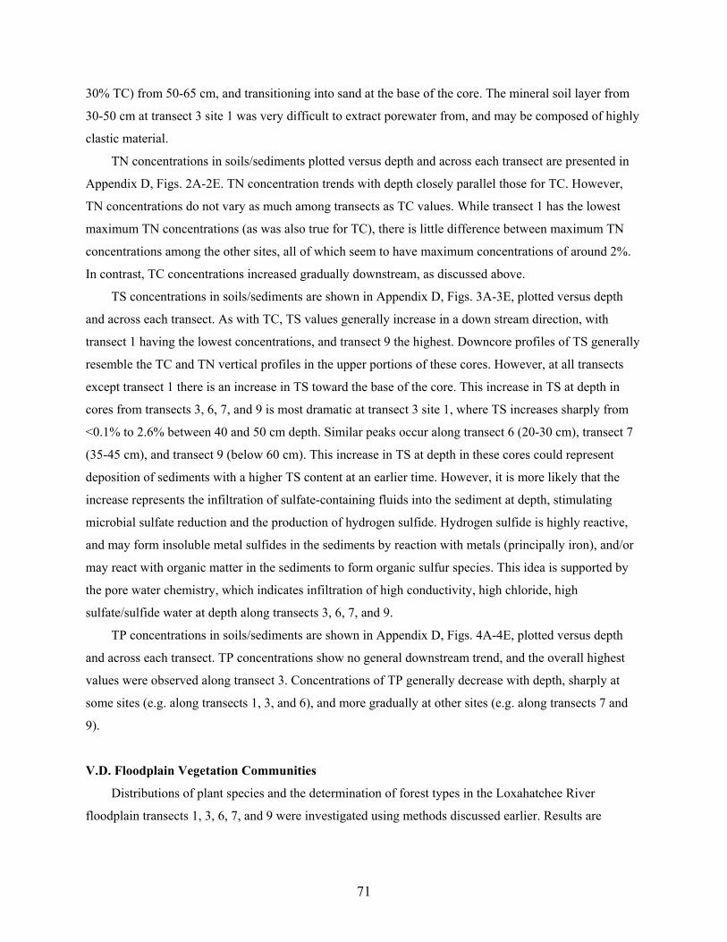
30% TC) from 50-65 cm, and transitioning into sand at the base of the core. The mineral soil layer from
30-50 cm at transect 3 site 1 was very difficult to extract porewater from, and may be composed of highly
clastic material.
TN concentrations in soils/sediments plotted versus depth and across each transect are presented in
Appendix D, Figs. 2A-2E. TN concentration trends with depth closely parallel those for TC. However,
TN concentrations do not vary as much among transects as TC values. While transect 1 has the lowest
maximum TN concentrations (as was also true for TC), there is little difference between maximum TN
concentrations among the other sites, all of which seem to have maximum concentrations of around 2%.
In contrast, TC concentrations increased gradually downstream, as discussed above.
TS concentrations in soils/sediments are shown in Appendix D, Figs. 3A-3E, plotted versus depth
and across each transect. As with TC, TS values generally increase in a down stream direction, with
transect 1 having the lowest concentrations, and transect 9 the highest. Downcore profiles of TS generally
resemble the TC and TN vertical profiles in the upper portions of these cores. However, at all transects
except transect 1 there is an increase in TS toward the base of the core. This increase in TS at depth in
cores from transects 3, 6, 7, and 9 is most dramatic at transect 3 site 1, where TS increases sharply from
<0.1% to 2.6% between 40 and 50 cm depth. Similar peaks occur along transect 6 (20-30 cm), transect 7
(35-45 cm), and transect 9 (below 60 cm). This increase in TS at depth in these cores could represent
deposition of sediments with a higher TS content at an earlier time. However, it is more likely that the
increase represents the infiltration of sulfate-containing fluids into the sediment at depth, stimulating
microbial sulfate reduction and the production of hydrogen sulfide. Hydrogen sulfide is highly reactive,
and may form insoluble metal sulfides in the sediments by reaction with metals (principally iron), and/or
may react with organic matter in the sediments to form organic sulfur species. This idea is supported by
the pore water chemistry, which indicates infiltration of high conductivity, high chloride, high
sulfate/sulfide water at depth along transects 3, 6, 7, and 9.
TP concentrations in soils/sediments are shown in Appendix D, Figs. 4A-4E, plotted versus depth
and across each transect. TP concentrations show no general downstream trend, and the overall highest
values were observed along transect 3. Concentrations of TP generally decrease with depth, sharply at
some sites (e.g. along transects 1, 3, and 6), and more gradually at other sites (e.g. along transects 7 and
9).
V.D. Floodplain Vegetation Communities
Distributions of plant species and the determination of forest types in the Loxahatchee River
floodplain transects 1, 3, 6, 7, and 9 were investigated using methods discussed earlier. Results are
71
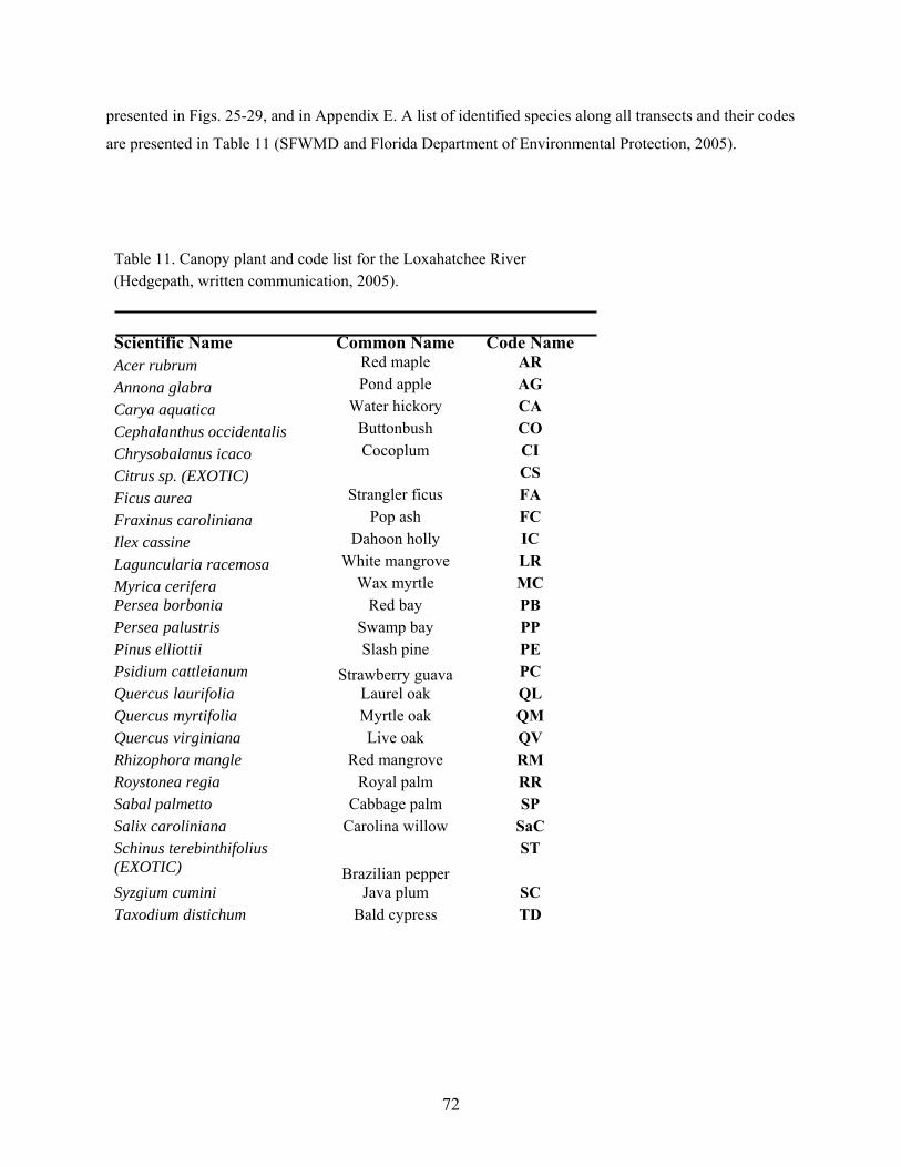
presented in Figs. 25-29, and in Appendix E. A list of identified species along all transects and their codes
are presented in Table 11 (SFWMD and Florida Department of Environmental Protection, 2005).
Table 11. Canopy plant and code list for the Loxahatchee River (Hedgepath, written communication, 2005). Scientific Name Common Name Code Name Acer rubrum Red maple AR Annona glabra Pond apple AG Carya aquatica Water hickory CA Cephalanthus occidentalis Buttonbush CO Chrysobalanus icaco Cocoplum CI Citrus sp. (EXOTIC) CS Ficus aurea Strangler ficus FA Fraxinus caroliniana Pop ash FC Ilex cassine Dahoon holly IC Laguncularia racemosa White mangrove LR Myrica cerifera Wax myrtle MC Persea borbonia Red bay PB Persea palustris Swamp bay PP Pinus elliottii Slash pine PE Psidium cattleianum Strawberry guava PC Quercus laurifolia Laurel oak QL Quercus myrtifolia Myrtle oak QM Quercus virginiana Live oak QV Rhizophora mangle Red mangrove RM Roystonea regia Royal palm RR Sabal palmetto Cabbage palm SP Salix caroliniana Carolina willow SaC Schinus terebinthifolius (EXOTIC) Brazilian pepper
ST
Syzgium cumini Java plum SC Taxodium distichum Bald cypress TD
72

Transect 1 is located just downstream of Lainhart Dam at Rivermile 14.7. This transect transverses
the north and south sides of the Northwest Fork with 15 10x10m plots (Figs. 12 and 13). It has several
elevation changes from 13.74 NGVD at the top of the mesic hammock to about 9.34 NGVD in the deeper
swamp areas and 5.44 NGVD in the river channel. The distribution of canopy species along this transect
is shown in Fig. 26. The exterior sides of transect 1 are dominated by several plots of upland and
hammock before dropping down into the floodplains as a cypress swamp that borders the riverbed. One
higher area adjacent to the bank of the river is classified as Rblh1 because of red maple within the plot
and water hickory just outside of the measured plot. Cabbage palm, live oak (Quercus virginiana), and
slash pine dominate the hammock and uplands plots while a stand of mostly very old bald cypress with an
average dbh of 49cm. dominate the Rsw1 plots. The smallest bald cypress has a dbh of 9.9cm. Because
the canopy is so well established in this area, and also because of high flow velocities, there is very little
indication of a subcanopy present at this transect. In addition, there are no indications of logging (i.e.
stumps only) in this area. Shrubs and groundcover in the Rsw1 areas are dominated by swamp lily
(Crinum americanum), tri-veined fern (Thelypteris interrupta), and downy shield fern (Thelypteris
dentata). The exotics elephant ear (Xanthosoma sagittifolium), and arrowhead vine (Syngonium
podophyllum) were also present as groundcover within the swamp community.
Fig. 26. Canopy species along transect 1 in the Loxahatchee River floodplain.
73
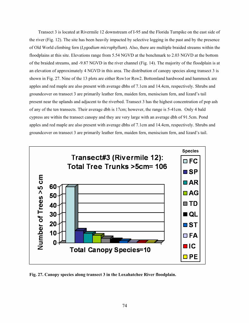
Transect 3 is located at Rivermile 12 downstream of I-95 and the Florida Turnpike on the east side of
the river (Fig. 12). The site has been heavily impacted by selective logging in the past and by the presence
of Old World climbing fern (Lygodium microphyllum). Also, there are multiple braided streams within the
floodplains at this site. Elevations range from 5.54 NGVD at the benchmark to 2.03 NGVD at the bottom
of the braided streams, and -9.87 NGVD in the river channel (Fig. 14). The majority of the floodplain is at
an elevation of approximately 4 NGVD in this area. The distribution of canopy species along transect 3 is
shown in Fig. 27. Nine of the 13 plots are either Rsw1or Rsw2. Bottomland hardwood and hammock are
apples and red maple are also present with average dbhs of 7.1cm and 14.4cm, respectively. Shrubs and
groundcover on transect 3 are primarily leather fern, maiden fern, meniscium fern, and lizard’s tail
present near the uplands and adjacent to the riverbed. Transect 3 has the highest concentration of pop ash
of any of the ten transects. Their average dbh is 17cm; however, the range is 5-41cm. Only 4 bald
cypress are within the transect canopy and they are very large with an average dbh of 91.5cm. Pond
apples and red maple are also present with average dbhs of 7.1cm and 14.4cm, respectively. Shrubs and
groundcover on transect 3 are primarily leather fern, maiden fern, meniscium fern, and lizard’s tail.
Fig. 27. Canopy species along transect 3 in the Loxahatchee River floodplain.
74
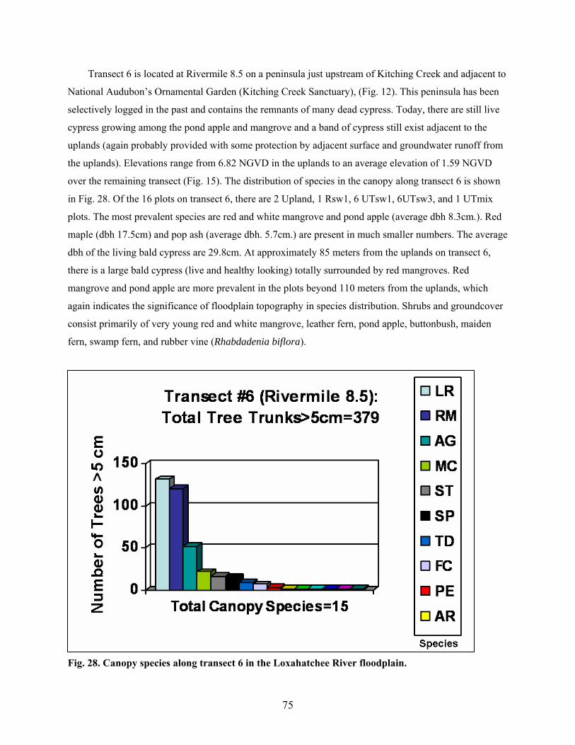
Transect 6 is located at Rivermile 8.5 on a peninsula just upstream of Kitching Creek and adjacent to
National Audubon’s Ornamental Garden (Kitching Creek Sanctuary), (Fig. 12). This peninsula has been
selectively logged in the past and contains the remnants of many dead cypress. Today, there are still live
cypress growing among the pond apple and mangrove and a band of cypress still exist adjacent to the
uplands (again probably provided with some protection by adjacent surface and groundwater runoff from
the uplands). Elevations range from 6.82 NGVD in the uplands to an average elevation of 1.59 NGVD
over the remaining transect (Fig. 15). The distribution of species in the canopy along transect 6 is shown
in Fig. 28. Of the 16 plots on transect 6, there are 2 Upland, 1 Rsw1, 6 UTsw1, 6UTsw3, and 1 UTmix
plots. The most prevalent species are red and white mangrove and pond apple (average dbh 8.3cm.). Red
maple (dbh 17.5cm) and pop ash (average dbh. 5.7cm.) are present in much smaller numbers. The average
dbh of the living bald cypress are 29.8cm. At approximately 85 meters from the uplands on transect 6,
there is a large bald cypress (live and healthy looking) totally surrounded by red mangroves. Red
mangrove and pond apple are more prevalent in the plots beyond 110 meters from the uplands, which
again indicates the significance of floodplain topography in species distribution. Shrubs and groundcover
consist primarily of very young red and white mangrove, leather fern, pond apple, buttonbush, maiden
fern, swamp fern, and rubber vine (Rhabdadenia biflora).
Fig. 28. Canopy species along transect 6 in the Loxahatchee River floodplain.
75
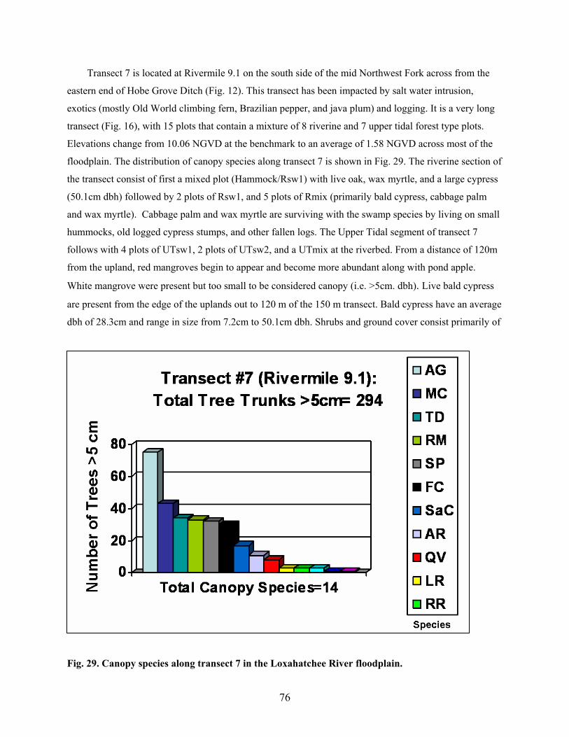
Transect 7 is located at Rivermile 9.1 on the south side of the mid Northwest Fork across from the
eastern end of Hobe Grove Ditch (Fig. 12). This transect has been impacted by salt water intrusion,
exotics (mostly Old World climbing fern, Brazilian pepper, and java plum) and logging. It is a very long
transect (Fig. 16), with 15 plots that contain a mixture of 8 riverine and 7 upper tidal forest type plots.
Elevations change from 10.06 NGVD at the benchmark to an average of 1.58 NGVD across most of the
floodplain. The distribution of canopy species along transect 7 is shown in Fig. 29. The riverine section of
the transect consist of first a mixed plot (Hammock/Rsw1) with live oak, wax myrtle, and a large cypress
(50.1cm dbh) followed by 2 plots of Rsw1, and 5 plots of Rmix (primarily bald cypress, cabbage palm
and wax myrtle). Cabbage palm and wax myrtle are surviving with the swamp species by living on small
hummocks, old logged cypress stumps, and other fallen logs. The Upper Tidal segment of transect 7
follows with 4 plots of UTsw1, 2 plots of UTsw2, and a UTmix at the riverbed. From a distance of 120m
from the upland, red mangroves begin to appear and become more abundant along with pond apple.
White mangrove were present but too small to be considered canopy (i.e. >5cm. dbh). Live bald cypress
are present from the edge of the uplands out to 120 m of the 150 m transect. Bald cypress have an average
dbh of 28.3cm and range in size from 7.2cm to 50.1cm dbh. Shrubs and ground cover consist primarily of
Fig. 29. Canopy species along transect 7 in the Loxahatchee River floodplain.
76
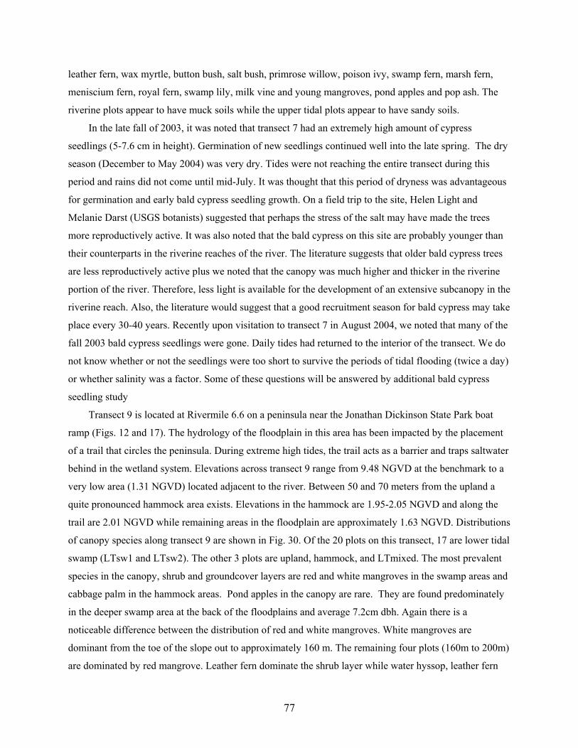
leather fern, wax myrtle, button bush, salt bush, primrose willow, poison ivy, swamp fern, marsh fern,
meniscium fern, royal fern, swamp lily, milk vine and young mangroves, pond apples and pop ash. The
riverine plots appear to have muck soils while the upper tidal plots appear to have sandy soils.
In the late fall of 2003, it was noted that transect 7 had an extremely high amount of cypress
seedlings (5-7.6 cm in height). Germination of new seedlings continued well into the late spring. The dry
season (December to May 2004) was very dry. Tides were not reaching the entire transect during this
period and rains did not come until mid-July. It was thought that this period of dryness was advantageous
for germination and early bald cypress seedling growth. On a field trip to the site, Helen Light and
Melanie Darst (USGS botanists) suggested that perhaps the stress of the salt may have made the trees
more reproductively active. It was also noted that the bald cypress on this site are probably younger than
their counterparts in the riverine reaches of the river. The literature suggests that older bald cypress trees
are less reproductively active plus we noted that the canopy was much higher and thicker in the riverine
portion of the river. Therefore, less light is available for the development of an extensive subcanopy in the
riverine reach. Also, the literature would suggest that a good recruitment season for bald cypress may take
place every 30-40 years. Recently upon visitation to transect 7 in August 2004, we noted that many of the
fall 2003 bald cypress seedlings were gone. Daily tides had returned to the interior of the transect. We do
not know whether or not the seedlings were too short to survive the periods of tidal flooding (twice a day)
or whether salinity was a factor. Some of these questions will be answered by additional bald cypress
seedling study
Transect 9 is located at Rivermile 6.6 on a peninsula near the Jonathan Dickinson State Park boat
ramp (Figs. 12 and 17). The hydrology of the floodplain in this area has been impacted by the placement
of a trail that circles the peninsula. During extreme high tides, the trail acts as a barrier and traps saltwater
behind in the wetland system. Elevations across transect 9 range from 9.48 NGVD at the benchmark to a
very low area (1.31 NGVD) located adjacent to the river. Between 50 and 70 meters from the upland a
quite pronounced hammock area exists. Elevations in the hammock are 1.95-2.05 NGVD and along the
trail are 2.01 NGVD while remaining areas in the floodplain are approximately 1.63 NGVD. Distributions
of canopy species along transect 9 are shown in Fig. 30. Of the 20 plots on this transect, 17 are lower tidal
swamp (LTsw1 and LTsw2). The other 3 plots are upland, hammock, and LTmixed. The most prevalent
species in the canopy, shrub and groundcover layers are red and white mangroves in the swamp areas and
cabbage palm in the hammock areas. Pond apples in the canopy are rare. They are found predominately
in the deeper swamp area at the back of the floodplains and average 7.2cm dbh. Again there is a
noticeable difference between the distribution of red and white mangroves. White mangroves are
dominant from the toe of the slope out to approximately 160 m. The remaining four plots (160m to 200m)
are dominated by red mangrove. Leather fern dominate the shrub layer while water hyssop, leather fern
77
Fig. 30. Canopy species along transect 9 in the Loxahatchee River floodplain.
and rubber vine dominate the groundcover. In August 2004, we returned to this transect to verify forest
type determinations and we noted that the majority of the cabbage palms that we had been recorded as
alive were now dead. The only remaining live cabbage palms were associated with the trail and the
hammock areas. Historically, the canopy on transect 9 was dominated by bald cypress; however, most of
these trees are dead now. In his 1967 plant survey of this transect, Taylor Alexander reported live bald
cypress at a frequency of 22.2 and a density of 0.39 (14 live and 28 dead). Red and white mangroves
were at a frequency and density of 52.8/1.31 and 36.1/2.64 (47 red and 95 white). In addition, Alexander
reported the presence of several other freshwater species in small numbers including sawgrass (Cladium
jamaicense), swamp lily, red bay, pop ash, red maple, and button bush. In a 1975 Jonathan Dickinson
State Park survey of 100 bald cypress trees on the peninsula, 71 were dead, 21 were healthy and 8 wer
e stressed. In our 2003 survey, there were no live cypress within Transect 9 and red and white mangroves
were at a frequency and density of 47/5.79 and 100/12.32. In an April 2004 resurvey of bald cypress on
the peninsula, 151 were dead, 7 were stressed and 3 were living. The three living bald cypress are
directly adjacent to or on the trail.
78
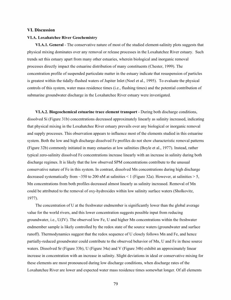
VI. Discussion
VI.A. Loxahatchee River Geochemistry
VI.A.1. General - The conservative nature of most of the studied element-salinity plots suggests that
physical mixing dominates over any removal or release processes in the Loxahatchee River estuary. Such
trends set this estuary apart from many other estuaries, wherein biological and inorganic removal
processes directly impact the estuarine distribution of many constituents (Chester, 1999). The
concentration profile of suspended particulate matter in the estuary indicate that resuspension of particles
is greatest within the tidally-flushed waters of Jupiter Inlet (Noel et al., 1995). To evaluate the physical
controls of this system, water mass residence times (i.e., flushing times) and the potential contribution of
submarine groundwater discharge in the Loxahatchee River estuary were investigated.
VI.A.2. Biogeochemical estuarine trace element transport - During both discharge conditions,
dissolved Si (Figure 31b) concentrations decreased approximately linearly as salinity increased, indicating
that physical mixing in the Loxahatchee River estuary prevails over any biological or inorganic removal
and supply processes. This observation appears to influence most of the elements studied in this estuarine
system. Both the low and high discharge dissolved Fe profiles do not show characteristic removal patterns
(Figure 32b) commonly initiated in many estuaries at low salinities (Boyle et al., 1977). Instead, rather
typical zero-salinity dissolved Fe concentrations increase linearly with an increase in salinity during both
discharge regimes. It is likely that the low observed SPM concentrations contribute to the unusual
conservative nature of Fe in this system. In contrast, dissolved Mn concentrations during high discharge
decreased systematically from ~350 to 200 nM at salinities < 1 (Figure 32a). However, at salinities > 5,
Mn concentrations from both profiles decreased almost linearly as salinity increased. Removal of Mn
could be attributed to the removal of oxy-hydroxides within low salinity surface waters (Sholkovitz,
1977).
The concentration of U at the freshwater endmember is significantly lower than the global average
value for the world rivers, and this lower concentration suggests possible input from reducing
groundwater, i.e., U(IV). The observed low Fe, U and higher Mn concentrations within the freshwater
endmember sample is likely controlled by the redox state of the source waters (groundwater and surface
runoff). Thermodynamics suggest that the redox sequence of U closely follows Mn and Fe, and hence
partially-reduced groundwater could contribute to the observed behavior of Mn, U and Fe in these source
waters. Dissolved Sr (Figure 33b), U (Figure 34a) and V (Figure 34b) exhibit an approximately linear
increase in concentration with an increase in salinity. Slight deviations in ideal or conservative mixing for
these elements are most pronounced during low discharge conditions, when discharge rates of the
Loxahatchee River are lower and expected water mass residence times somewhat longer. Of all elements
79
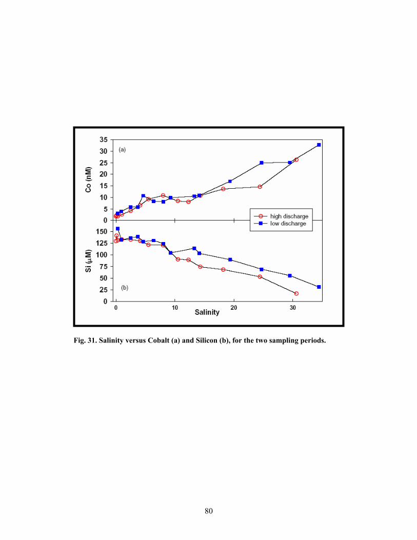
Fig. 31. Salinity versus Cobalt (a) and Silicon (b), for the two sampling periods.
80
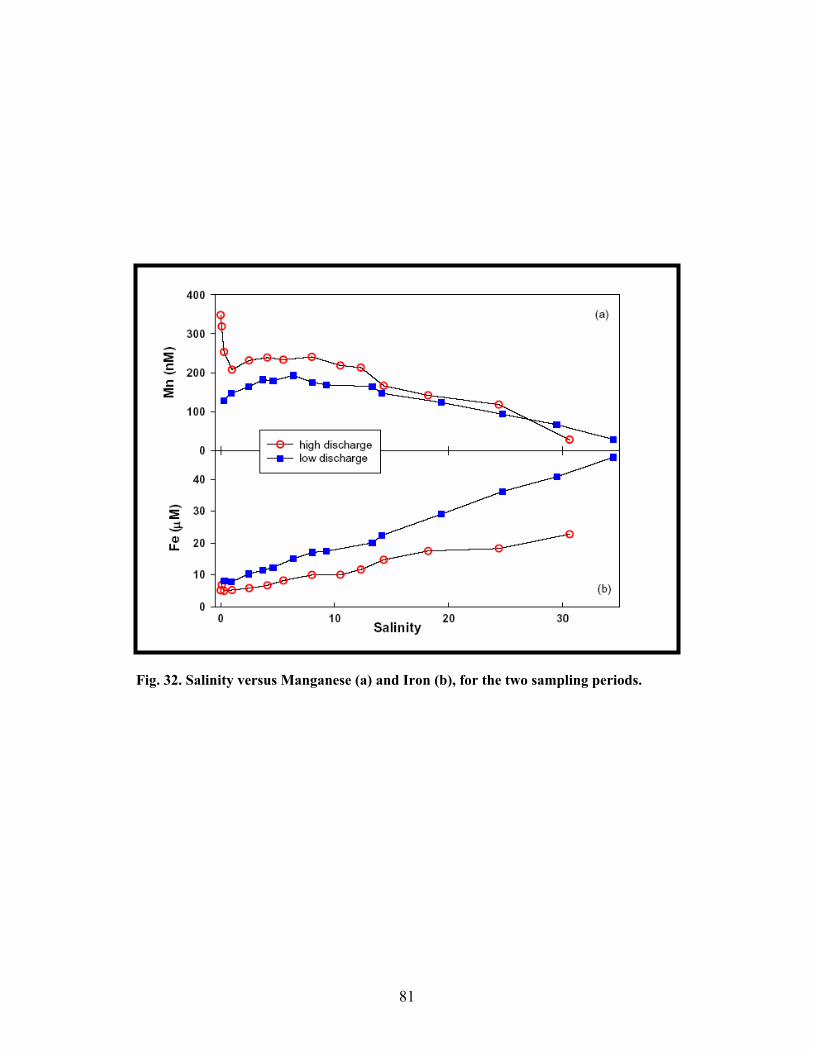
Fig. 32. Salinity versus Manganese (a) and Iron (b), for the two sampling periods.
81
Fig. 33. Salinity versus Barium (a), and Strontium (b), for the two sampling periods.
Fig. 33. Salinity versus Barium (a), and Strontium (b), for the two sampling periods.
82
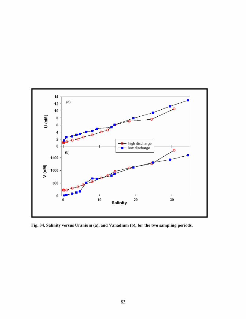
Fig. 34. Salinity versus Uranium (a), and Vanadium (b), for the two sampling periods.
83
studied, dissolved Ba concentrations (Figure 33a) in the two endmember samples varied the most between
the two discharge stages. Cobalt concentrations (Figure 30a) were lowest (2-3 nM) in the fresh-
watersurface samples and increased to above 30 nM in the most saline samples. The general absence of
Co in the head waters of this river system implies that the source waters, which may be a composite of
reduced groundwater and surface runoff, are still not notably impacted by the rapid and wide-spread
development adjacent to the Loxahatchee River watershed.
Dissolved organic carbon (DOC) concentrations show similar decreasing trends with respect to an
increase in salinity for both river discharge conditions (Figure 19b). DOC in the freshwater endmember
samples ranged from ~1000 µM (low discharge) to ~1200 µM (high discharge), and decreased in
concentration to just above 100 µM at the high salinity (34.42) endmember (low discharge). Observations
in non-linear estuarine DOC mixing were most pronounced during both discharge regimes at salinities
between 0 and 15. DOC values in the upper Loxahatchee River estuary are elevated considerably relative
to ‘average’ DOC values for small streams (Thurman, 1985). In spite of the general paucity of suspended
particulate matter present in the estuarine water column, the observed decrease in DOC concentrations
with an increase in salinity may be attributed to the classic removal of terrestrial dissolved organic matter
(i.e., aggregation, coagulation) during estuarine transport.
VI.B. Groundwater Flux in Loxahatchee River
VI.B.1. Ra-derived estuarine water mass ages – The construction of a Ra-derived groundwater
flux model for the Loxahatchee River and its estuary, which builds upon a mass balance of source and
removal terms, relies on the derivation of an accurate estuarine residence time. The residence time of a
water parcel transported through an estuary, Tr, can be defined as a composite of various physical
parameters such as the hydraulic gradient, the rate and seasonality of stream flow, the tidal range and
amplitude, as well as anthropogenic demand on coastal fresh water resources. Such a residence time can
be calculated using either physical (Pilson, 1985) volume and area estimates (i.e., tidal prism) or isotopic
tracers (Charette et al., 2001). In the Loxahatchee River estuary, the residence time of water calculated
using a best-estimate for the tidal prism volume (tpvol = 3.98 x 10⁶ m3; McPherson et al., 1982), the
surface volume (6.29 x 10⁶ m3) and the tidal period (tper = 1.9 d-1) is less than one day, ~0.8 d. Such a
short residence time confirms the energetic exchange that occurs through Jupiter Inlet, and implies rapid
estuarine flushing rates into the Atlantic Ocean.
To alternatively calculate Tr values using Ra isotopes, an approach that compares excess isotopic
ratios (224Ra/xs228Ra) in surface waters to such ratios in groundwater can be expressed as (after Moore,
2000; Charette et al., 2002):
[224Ra/xs228Ra]estu = [224Ra/xs228Ra]gwe-λ224Tr (1)
84
Where [224Ra/xs228Ra]estu represents the observed activity ratio of the estuarine sample, [224Ra/xs228Ra]gw
the average activity ratio in groundwater, and λ224 is the decay constant for 224Ra, 0.1894 d-1. Excess Ra
activities are calculated here by simply subtracting an oceanic endmember activity (e.g., 228Ra = 6.71
dpm 100 L-1) from the observed activities. Rearranging Eq. 1 allows one to solve for Tr:
Tr = ln[(224Ra/xs228Ra)gw – (224Ra/xs228Ra)estu] / λ224 (2)
For each station, a residence time was calculated based on Eq. 2 using average (224Ra/xs228Ra)gw
values of 2.63 (high discharge) and 2.58 (low discharge). The range in calculated residence time estimates
spans from ~0.44 to 1.39 days, for both sampling efforts. Such individual residence time estimates were
averaged to yield composite estuarine Tr rates of 0.97 d and 0.83 d for high and low flow conditions,
respectively, which are in close agreement with those calculated via the tidal prism method. Calculated
residence times are shorter at the high salinity samples for both sampling efforts and suggest that such a
technique might be sensitive enough to resolve local fluctuations in the estuarine flushing efficiency.
VI.B.2. Ra-derived groundwater discharge - To quantify the role of groundwater discharge to the
Loxahatchee River and its estuary, an equation can be written that identifies known source terms of Ra in
an estuary. The calculated activity of Rac may thus be defined as the sum of the fractional contribution of
Ra present in seawater (Ras), river water (Rar), as well as the fractional contribution of Ra desorbed from
riverine particulates (Rades) (Krest et al., 1999; Kelly and Moran, 2002):
Rac = ƒ(Ras) + (1-ƒ)(Rar) + ((1-ƒ)Rades)(1-e[-Sestu/ξ]) (3)
Here, Sestu denotes the sample salinity, and ξ represents the salinity at which the particulate-bound Ra
activity is thought to be reduced to e-1 of its initial activity due to a change in ionic strength; salinity = 5‰
(Krest et al., 1999; Kelly and Moran, 2002). In Eq. 3, the term f represents the fractional contribution of a
sample’s salinity derived by the seawater and freshwater endmembers (Krest et al., 1999) as follows:
ƒ = (Sestu – Sr) / (Ssea – Sr) (4)
where Ssea and Sr represent seawater and freshwater endmember salinities, respectively. Applying Eq. 4,
one can quantitatively evaluate the relative contribution of each of the Ra source terms against observed
Ra distributions. In general, such calculated activities are consistently less than observed activities present
in the estuary for all four Ra isotopes, which suggests that either Ra is being actively advected into the
estuarine water column by groundwater discharge, and/or, Ra production via the decay of parent Th
ubiquitously-present in bottom sediment contributes substantially to the estuarine Ra mass balance.
To demonstrate that the production or regeneration rate of Ra within Loxahatchee River estuary
bottom sediments is a minor contributor to the overall Ra mass balance, we collected six bottom sediment
samples (3 sites per cruise) from sites within the entire estuary (salinity 0 to 34‰) that represent the
spectrum of geologic strata present in this estuary. An average production rate of 226Ra, derived from the
disequilibrium between 226Ra and its immediate parent, 230Th (t½ = 1.4 x 10¹⁰ yr), and integrated over
85
the entire Loxahatchee River estuary area was calculated to be 1.45 x 10⁴ dpm d-1. Such a calculation
assumes that ~75 % of the sediment-bound Ra is available for desorption and subsequent transport into
estuarine waters (Rama and Moore, 1996). By deriving estimates for Rac, Tr and Rades, one can then
establish an equation the describes that mass balance of excess 226Ra in the estuary (Charette et al., 2001;
Kelly and Moran, 2002) as follows: 226Raxs = [(226Raave – 226Rasea) *Vestu / Tr] – [226Rar *Qr] – [226Rades *Aestu] (5)
where 226Raave is the average measured activity in the estuary, 226Rasea is the activity in the adjacent
Atlantic Ocean that can be tidally-exchanged through Jupiter Inlet, Tr is the Ra-derived estuarine
residence time calculated from Eq. 2, Vestu and Aestu are volume and area estimates for the estuary,
respectively (Russell and McPherson, 1984), Qr is the river discharge rate, and 226Rades is the calculated
estuarine-wide regeneration rate of 226Ra from bottom sediments.
The calculated estuarine 226Raxs activity or removal flux using Eq. 5 ranged 2.89 x 10⁸ to 6.37 x 10⁸
dpm d-1, during high and low river discharge conditions, respectively. To confirm such estimates, one can
also calculate such estuarine removal flux estimates using tidal prism characteristics for the Loxahatchee
River estuary and calculated Raxs values (Kelly and Moran, 2002), such that:
Raxs = Raobs - Rac (6)
where Raobs represents the observed estuarine Ra activities and Rac the calculated activities, after Eq. 3,
and, 226Raxs = [Raxs *tper *tpvol *10] (7).
In Eq. 7, 226Raxs is expressed as a function of the tidal prism volume (tpvol), the tidal period (tper) and
the calculated excess Ra present in the estuarine water column, and ranged from 0.13 to 3.48 x 10⁸ dpm
d-1, during both low and high discharge, respectively. During high-flow conditions, the two independent
methods provide removal flux estimates that are in close agreement. Slight differences in the two
calculated removal flux estimates during low discharge are likely influenced by the lower 226Ra activities
observed at salinities between 0.92 to 3.69‰. Such results validate some of the inherent assumptions in
these groundwater discharge techniques, which imply, for example, that the Ra-derived residence times
are truly representative of the entire estuary, or that the endmember Ra activities (including ground-water
activities) are reasonably constant for the entire duration of the sampling effort.
To quantify the rate of groundwater discharge for the Loxahatchee River estuary, the estuarine
removal flux estimate derived using Eqs. 5 or 7 is assumed to be in steady-state with respect to the
groundwater input. Therefore, one can calculate an estuarine-wide groundwater discharge rate, as follows,
SGD = (226Raxs/226RaGW) (8)
where 226RaGW represents an average groundwater 226Ra activity per sampling cruise. Based on the tidal
prism approach (Eq. 7), the Ra-derived input of groundwater to the estuary (Table 12) during high
86
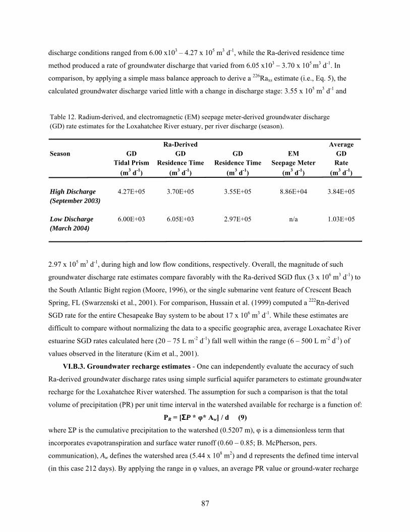
discharge conditions ranged from 6.00 x10³ – 4.27 x 10⁵ m3 d-1, while the Ra-derived residence time
method produced a rate of groundwater discharge that varied from 6.05 x10³ – 3.70 x 10⁵ m3 d-1. In
comparison, by applying a simple mass balance approach to derive a 226Raxs estimate (i.e., Eq. 5), the
calculated groundwater discharge varied little with a change in discharge stage: 3.55 x 10⁵ m3 d-1 and
Table 12. Radium-derived, and electromagnetic (EM) seepage meter-derived groundwater discharge (GD) rate estimates for the Loxahatchee River estuary, per river discharge (season).
Ra-Derived AverageSeason GD GD GD EM GD
Tidal Prism Residence Time Residence Time Seepage Meter Rate(m3 d-1) (m3 d-1) (m3 d-1) (m3 d-1) (m3 d-1)
High Discharge 4.27E+05 3.70E+05 3.55E+05 8.86E+04 3.84E+05(September 2003)
Low Discharge 6.00E+03 6.05E+03 2.97E+05 n/a 1.03E+05(March 2004)
2.97 x 10⁵ m3 d-1, during high and low flow conditions, respectively. Overall, the magnitude of such
groundwater discharge rate estimates compare favorably with the Ra-derived SGD flux (3 x 10⁶ m3 d-1) to
the South Atlantic Bight region (Moore, 1996), or the single submarine vent feature of Crescent Beach
Spring, FL (Swarzenski et al., 2001). For comparison, Hussain et al. (1999) computed a 222Rn-derived
SGD rate for the entire Chesapeake Bay system to be about 17 x 106 m3 d-1. While these estimates are
difficult to compare without normalizing the data to a specific geographic area, average Loxachatee River
estuarine SGD rates calculated here (20 – 75 L m-2 d-1) fall well within the range (6 – 500 L m-2 d-1) of
values observed in the literature (Kim et al., 2001).
VI.B.3. Groundwater recharge estimates - One can independently evaluate the accuracy of such
Ra-derived groundwater discharge rates using simple surficial aquifer parameters to estimate groundwater
recharge for the Loxahatchee River watershed. The assumption for such a comparison is that the total
volume of precipitation (PR) per unit time interval in the watershed available for recharge is a function of:
PR = [ΣP * φ* Aw] / d (9) where ΣP is the cumulative precipitation to the watershed (0.5207 m), φ is a dimensionless term that
incorporates evapotranspiration and surface water runoff (0.60 – 0.85; B. McPherson, pers.
communication), Aw defines the watershed area (5.44 x 10⁸ m2) and d represents the defined time interval
(in this case 212 days). By applying the range in φ values, an average PR value or ground-water recharge
87
rate to the Loxahatchee river estuary is estimated to be 1 x 10⁶ m3 d-1. In spite of the inherent simplicity in
such calculations, it is encouraging that this recharge estimate is slightly greater than the average Ra-
derived ground-water discharge rate. The difference in these two flux estimates may be due to some small
component of groundwater that discharges directly into the Loxahatchee River estuary from a deeper
aquifer. VI.B.4. Electromagnetic seepage meter measurements - In order to validate the calculated Ra-
derived submarine groundwater discharge rates for this estuary, we also deployed an autonomous
electromagnetic (EM) seepage meter (Rosenberry and Morin, 2004; Swarzenski et al., 2004) at the
confluence of Kitching Creek and the Loxahatchee River estuary, close to 12 km upstream from Jupiter
Inlet (Fig. 11). An advantage of such an automatic instrument is that the wide range of bi-directional
sediment/water interface exchange rates that can be measured rapidly and precisely can provide a precise,
although very point-specific, groundwater/surface water exchange rate. There are well-known limitations
in the accuracy and interpretation of some manual seepage meter results (Lee, 1977; Tanaguchi and
Fukuo, 1993), and these can potentially be identified and minimized using autonomous instruments such
as the EM seepage meters. Nonetheless, seepage meter results should be interpreted cautiously, as here in
this system they record groundwater/surface water exchange conditions at only one site. For a 2-day
deployment in September 2003, a 10-min. averaged SGD rate of 1.71 cm d-1 yielded an estuarine-wide
upward submarine ground-water discharge rate of ~ 0.9 x 10⁵ m3 d-1; a value very close in magnitude to
the Ra-derived estimate. Thus, it appears that two independent techniques provide at least a first-order,
reliable estimate of submarine ground-water discharge for this estuary. Observed variations in the
calculated estimates of submarine ground-water discharge from these two very different techniques may
result from the EM seepage work being only from one site in the estuary, while the Ra-derived estimates
incorporate data that was derived from samples collected across the entire salinity gradient.
VI.B.5. Surface water Rn-222 activities - It has been repeatedly shown that 222Rn (t1/2 = 3.8 d)
activities, when measured in surface waters, may provide useful insight into rates and magnitudes of
groundwater/surface exchange (Cable et al., 1996; Corbett et al., 1999; Burnett et al., 2001, Burnett and
Dulaiova, 2003, Oliveira et al., 2003; Lambert and Burnett, 2003; Purkl and Eisenhauer, 2004). To
evaluate the contribution of groundwater discharge to the Loxahatchee River estuary using 222Rn as a
tracer, we surveyed the surface water column using six commercial radon detectors, plumbed in parallel
through one air/water exchanger (Burnett et al., 2001; Burnett et al., 2003; Swarzenski et al., 2004). These
new techniques have greatly simplified the collection and subsequent detection of Rn, such that one now
can obtain almost real-time excess 222Rn activities in situ.
From a river survey initiated close to the Atlantic Ocean at Jupiter Inlet, 222Rn activities increased
rapidly from near-background activities (~2.5 dpm L-1) to values in excess of 28 dpm L-1 in the
88
Loxahatchee River close to the Kitching Creek confluence (Figure 23). The near-symmetrical shape of
the Rn profile as a function salinity or distance from Jupiter Inlet suggests that submarine ground-water
discharge occurs prevalently in the headwaters of the river system, and that the short residence time
within the estuary (< one day) and the ubiquitous nature of SGD upstream, appear to offset any expected
tidal control on SGD rates. The 222Rn profile in the Loxahatchee River estuary very clearly demonstrates
the utility of this tracer to identify specific regions of a river/estuary that are active sites of submarine
groundwater discharge.
VI.B.6. Subsurface streaming resistivity profiling measurements - Streaming resistivity profiling
techniques were used in the Loxahatchee River estuary to investigate subsurface fresh water/saltwater
interface dynamics in light of the enriched 222Rn activities in the source waters of the Loxahatchee River.
One example of an inverse modeled streaming resistivity profile result from the June 2004 survey is
shown in Fig. 35; a) depicts a East-West transect line close to Jupiter Inlet, while b) illustrates a transect
line upstream in the vicinity of the Kitching Creek/Loxahatchee River confluence. Sediments that are
saturated in freshened interstitial water masses generally have higher resistivity ranges (up to 20 Ω m),
while more saline interstitial waters would correspond to lower resistivity values. If one assumes (as a
first approximation) that the sediments underlying the Loxahatchee River estuary are homogenous in
composition, and that down-core porosity is held constant, then an observed shift towards higher
resistivity would imply freshened pore waters. Such streaming resistivity results clearly show that the
sediments underlying the Loxahatchee River estuary reflect the dynamic nature of the
freshwater/saltwater interface; upstream at Kitching Creek, the sediments show little influence of
saltwater, while in the vicinity of Jupiter Inlet, the sediments are largely seawater-saturated. VI.B.7. Groundwater-derived nutrient fluxes - The delivery and potential diagenetic
transformation of select nutrients during submarine ground-water discharge may negatively impact
coastal ecosystems (Howes and Weiskel, 1996; Harvey and Odum, 1990; Giblin and Gaines, 1990; Krest
et al., 2000; Gobler and Sandu-Wilhelmy, 2001; Crotwell and Moore, 2003; Slomp and Cappellen, 2004).
For example, N and P concentrations are often elevated in coastal groundwater relative to river water, and
the stoichiometry of N:P in submarine groundwater most often diverges drastically from the Redfield
ratio (16:1) (Capone and Bautista, 1985; Lapointe et al., 1990; Valiela et al., 1990; Weiskel and Howes,
1992; Gallagher et al., 1996; Corbett et al., 1996,1997; LaRoche et al., 1997; Herrera-Silveira, 1998;
Miller and Ullman, 2004). By applying our calculated Ra-derived submarine groundwater discharge rate
estimates, one can evaluate the groundwater-derived nutrient inputs to the Loxahatchee River estuary per
discharge period (Table 13), using average ground-water nutrient concentrations. We used NH4+ and PO4
-
3 values representing a composite average (n > 50) per river discharge stage that were collected from a
series of vertical porewater sites in the Loxahatchee River floodplain along a series of transects (1,3,6,7,
89
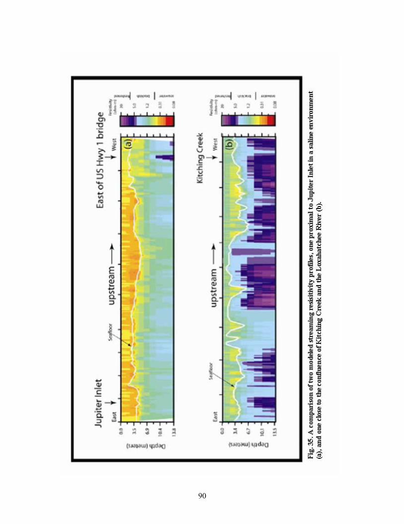
90
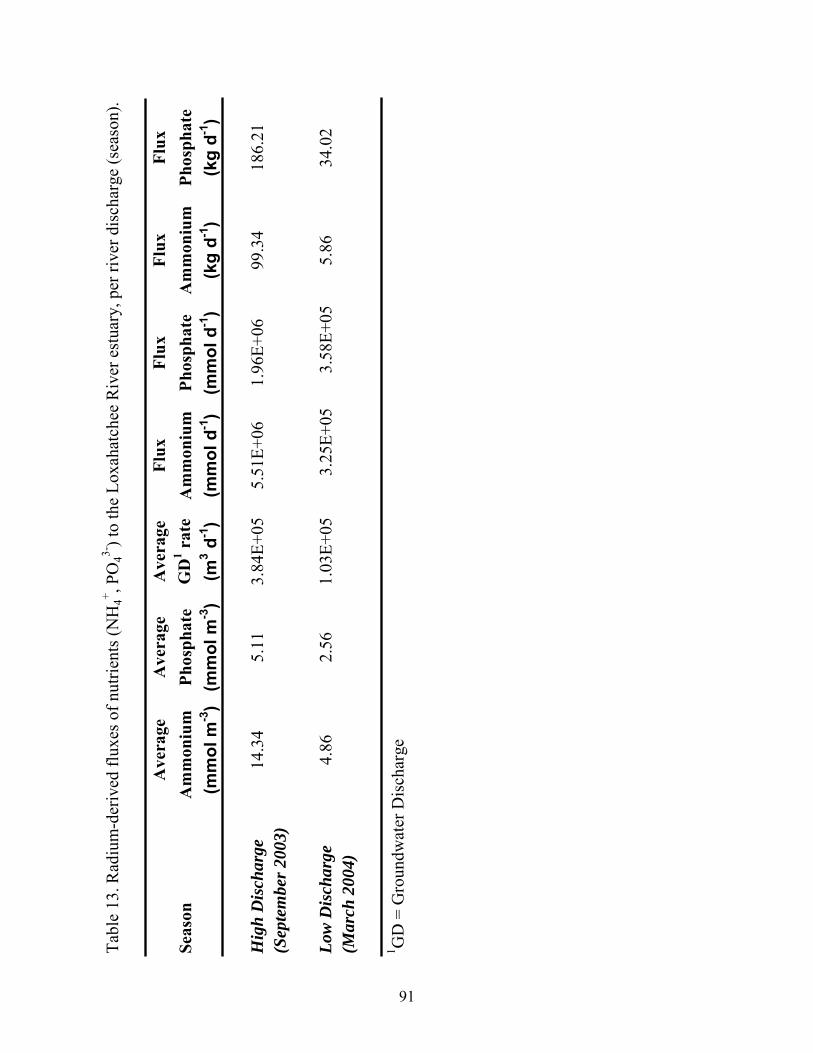
Tabl
e 13
. Rad
ium
-der
ived
flux
es o
f nut
rient
s (N
H4+ , P
O43-
) to
the
Loxa
hatc
hee
Riv
er e
stua
ry, p
er ri
ver d
isch
arge
(sea
son)
.
Ave
rage
Ave
rage
Ave
rage
Flux
Flux
Flux
Flux
Seas
onA
mm
oniu
mPh
osph
ate
GD
1 rat
eA
mm
oniu
mPh
osph
ate
Am
mon
ium
Phos
phat
e3 d
-1)
(mm
ol d
-1)
(kg
d-1)
(kg
d-1)
(mm
ol m
-3)
(mm
ol m
-3)
(m(m
mol
d-1
)
Hig
h D
isch
arge
14.3
45.
113.
84E+
055.
51E+
061.
96E+
0699
.34
186.
21(S
epte
mbe
r 200
3)
Low
Dis
char
ge4.
862.
561.
03E+
053.
25E+
053.
58E+
055.
8634
.02
(Mar
ch 2
004)
1 GD
= G
roun
dwat
er D
isch
arge
91
and 9), as discussed earlier in this report. The floodplain porewater nutrients likely represent a significant
fraction of the total nutrients discharged into the Loxahatchee River system from groundwater, given the
large size of the floodplain compared to the river channel. However, the floodplain porewater does not
represent the only source of subsurface nutrients to the river and estuary, and we have no data, for
example, for nutrient concentrations in river bottom sediment porewater. Thus, the nutrient discharge
estimates calculated here represent only the estimated discharge from groundwater sourced within the
floodplain. From such porewater values, the average NH4
+ concentration ranged from 4.86 to 14.34 mmol m-3
during low and high discharge, respectively, while PO4-3 ranged from 2.56 to 5.11 mmol m-3, respectively.
Multiplying these average nutrient concentrations by seasonally-averaged SGD rates, yields daily NH4+
fluxes into the estuary that range from 0.33 – 5.51 x 10⁶ mmol (6.3 x 101 – 1.1 x 10³ µmol m-2 d-1),
depending on the river discharge stage. The flux of PO4-3 similarly ranged from 0.36 – 1.96 x 10⁶ mmol
(6.9 x 101 – 3.8 x 10² µmol m-2 d-1) per day, during low and high discharge, respectively.
Such estimates for nutrient transport into the Loxahatchee River estuary may be compared to other
SGD-influenced coastal waters. For example, in Waquoit Bay, MA, Charette et al. (2001) observed a
SGD- derived DIN (NO3- + NH4
+) flux of about 550 µmol m-2 d-1. In a recent review of SGD-enhanced
nutrient transport, Slomp and Capellen (2004) report that the range in N-flux extends from 160 µmol m-2
d-1 off Hawaii (Garrison et al., 2003) to 72,000 µmol m-2 d-1 in a small estuary off New England (Portnoy
et al., 1998). Comparable SGD-derived P-flux estimates are much more infrequent, and range from <1.0
µmol m-2 d-1 in Florida Bay (Corbett et al., 1999) to 900 µmol m-2 d-1 off North Inlet, NC (Krest et al.,
2000). The range in reported nutrient flux estimates reflects the underlying geology as well as potential
anthropogenic perturbations.
VI.C. Water Chemistry - Loxahatchee River Floodplain
Perhaps the factor of most interest in the surface and pore water data is the presence of high ionic
strength water at depth in the sediment pore water at most sites. At the beginning of this study, it was
hypothesized that the loss of freshwater vegetation (notably Taxodium) and replacement by mangrove
swamp forest along portions of the Loxahatchee River was due to saltwater intrusion up the river. This
saltwater intrusion was thought to be a result of the opening of Jupiter Inlet, and net decreased freshwater
flow within the Loxahatchee River watershed resulting from urbanization and development. Saltwater
intrusion was visualized as occurring by saltwater movement up the river, and surface overflow into the
floodplain. However, this is not what is observed. While it does appear that high ionic strength water is
observed as far upstream as Transect 3, this water appears at depth in pore water, not at the surface. Even
at the most downstream location (transect 9), more saline water appears at depth. The high ionic strength
92
water at depth cannot be a result of evaporative concentration during the dry season, because of the high
sulfate concentrations. Sulfate resident for a period of time would be quickly reduced by microbial sulfate
reduction to sulfide, under the anoxic conditions present in the sediments. The high sulfate levels at depth,
therefore, suggest a continuous source of new sulfate from below. Two possibilities might explain the
more saline water at depth in the floodplain pore water: (1) saltwater moving upstream as a saltwater
wedge through the permeable sand underlying the surficial sediments, and (2) high ionic strength
groundwater in the floodplain. The difficulty with the groundwater explanation is that the groundwater
from upland wells (e.g. wells at the upland edge of the floodplain) has very low ionic strength. Thus,
results from the brief floodplain study suggest that saltwater is moving upriver at depth in a kind of tidal
wedge, with less dense fresher water at the surface. However, this result is not definitive, and further
study of this is needed.
Preliminary nutrient results from the floodplains showed that primary production may be N-limited
rather than the more usual P-limitation (see section V.B.6). The relatively low N/P values may reflect
both denitrification within the floodplain sediments and a source of excess P within the system. In
general, the major limiting factor in riparian ecosystems is the physical stress of inadequate root oxygen
during flooding rather than an inadequate supply of minerals (Spink and Rogers, 1996). Nitrate levels
along Transect 1 were relatively low (<10µg/l), while phosphate levels were high (exceeding 1,300 µg/l
in some intervals).
Cations and anions showed overall large differences among the different transects. Upriver transects
(Transects 1, 3, and 7) had cations dominated by calcium and anions dominated by alkalinity (probably
predominantly bicarbonate). In contrast, downstream Transects 6 and 9 had cations dominated by sodium
and magnesium, and anions dominated by chloride, and to a lesser extent sulfate. There was a net cationic
charge deficit at all sites, in pore water and surface water, and in both the wet and dry season. For
example, Transect 1 surface water had average anionic charge of about 4.24 and 6.69 meq/l in the wet and
dry seasons, respectively, but average cationic charge of only 3.26 and 3.95 meq/l in the wet and dry
seasons, respectively. Pore water along Transect 1 had average anionic charge of 6.32 (wet season) and
12.4 (dry season) meq/l, compared to average cationic charge of 5.23 (wet season) and 7.98 (dry season)
meq/l. Similar anionic/cationic charge imbalances were observed along other transects for the measured
species. There are several possible explanations for the observed charge imbalance, including excess
cationic charge in absorbed species on the solid phase, and cationic species (e.g. iron) not measured in
this study.
93
VI.D. Sediment Geochemistry - Floodplain
Sediments in the Loxahatchee River floodplain vary from an organic matter-rich soil, to a true peat
progressing downstream. This organic matter-rich soil/peat overlies sand, and varies in thickness from 30
cm to nearly 100 cm, depending on the Transect and location. The downstream locations (Transects 6, 7,
and 9) generally have thicker and more organic matter-rich soil/sediment overlying the underlying sand,
reflecting the twice daily tide effects at these transects. The more upriver transects (1 and 3) do not
experience twice daily tidal inundation in the floodplain. The floodplain along the upriver transects have
virtually no surface water present during the November-May dry season, and the soils here thus are more
subject to oxidation of deposited organic matter.
Concentrations of TC, OC, TN, TP and TS in soils/sediments along Transects 1, 3, and 6 generally
decrease with increasing depth, reflecting both an increase in admixed mineral matter (sand, silt, clay),
and microbial decomposition of deposited organic matter (Appendices C and D). The more peat-like
deposits along Transects 7 and 9 show unsystematic profiles of TC, OC, TN, TP, and TS concentrations
with increasing depth, largely reflecting differential influx of mineral matter material deposited from the
river. Subsurface peaks in TS observed at some sites likely reflect deposition of sulfide mineral phases
(monosulfides, and disulfides), and reaction of sulfide with organic matter to form organic sulfur
compounds. The deposition of the sulfide mineral phases and formation of organic sulfur phases at depth
in these soils/sediments appear to be driven by high ionic strength water containing sulfate at depth in
pore water. Under the generally anoxic conditions present, microbial sulfate reduction produces sulfide as
a metabolic byproduct, and the reactive sulfide may form the sulfide mineral and organic sulfur
compounds contributing to the high TS in the soils/sediments. This production of TS from high levels of
sulfate and sulfide in deep pore water was observed as far north as Transect 3.
VI.E. Water Levels, Water Quality and Vegetation Changes in the Floodplain
Three distinct reaches (riverine, and upper and lower tidal) and four major forest community types
(swamp, bottomland hardwood, hammock, and uplands) were identified on the floodplains of the
Northwest Fork of the Loxahatchee River (SFWMD, 2002). Riverine floodplain communities were
predominately bald cypress and bald cypress/pop ash swamps with mixed areas of low bottomland
hardwood and hammock. Younger subcanopies were present in disturbed areas and were evident by their
smaller trunks (i.e. diameter at breast height). In impacted areas where large trees were historically
logged, it appears that bald cypress are being replaced by pop ash and bottomland hardwood species that
require shorter hydroperiods and are faster growing. Very few bald cypress seedlings or saplings are
noted in the shrub and groundcover of the riverine reach. This could be a factor of light availability, low
nutrients, or the age of the trees.
94
The Comprehensive Everglades Restoration Plan (North Palm Beach County) calls for the
improvement of the quality, quantity, timing, and distribution of water delivery to the the NW Branch
(Fork) of the Loxahatchee River in order to enhance and restore the remaining ecosystem. For restoration
and enhancement measures in this reach, the goal is to promote the sustainable health of the existing
forest types (including canopy, subcanopy, and groundcover components of the community), and target
species by improving wet and dry season hydrological conditions and reducing sedimentation. In the
future, the riverine reach will require new canopy recruitment to replace the older generation of deciduous
trees. Future community composition of the shrub and ground cover species in the swamp habitats will
likely reflect the improved hydrological conditions. Transitional and upland species should be reduced
and or eliminated from the swamp habitat areas.
Upper tidal floodplain communities are dominated by mixed swamps and hammock. Although
bottomland hardwood indictor species were present, distinct areas of bottomland hardwood were not
present probably due to the lack of topographical change and low existing elevations. Hammock and
bottomland hardwood species are adapting to this ecosystem by growing on hummocks, cypress stumps
and fallen logs. Where present on the riverine plots, bald cypress comprised most of the canopy with pop
ash and pond apple present as subcanopy. Canopy in the upper tidal plots were comprised of
predominantly pond apple and red and white mangroves. Bald cypress and pond apple seedlings and
saplings were noted in the shrub and ground cover vegetation of the upper tidal reach. With regards to
restoration and enhancement measures in the upper tidal reach, the goal of the Restoration Plan would be
to promote the increase in abundance and distribution of freshwater forest species in the canopy,
subcanopy, shrub and groundcover components of the floodplain community and reduce the spread of
mangroves and exotic plant species.
In the lower tidal floodplain communities the canopy was composed of mostly red and white
mangrove, depending on elevation. There was no evidence of freshwater seedling/sapling production in
the lower tidal areas, with the exception of pond apple, which appears to be salt tolerant. Therefore,
reducing salt concentrations and increasing freshwater inundation will likely promote healthier
sustainable habitats within the swamp and hydric hammock areas. Reducing the recruitment of new
individuals of mangrove and controlling exotic species may also assist in establishing sustainable swamp
and hydric hummock habitat.
The dominant canopy species (exotic and native species) are listed in Table 11. The native species
reflect those species that represent best restoration targets for each forest community. Their current
abundance is expressed in the vegetation transect histograms in Figs 25-29. Bald cypress would typically
be the dominant species with some pop ash in the swamp communities. Low bottomland hardwood
communities would typically be dominated by red maple, buttonbush, swamp bay, and Carolina willow,
95

while high bottomland hardwood would be dominated by water hickory, laurel oak, dahoon holly and
cocoplum. Hydric hammock communities should be dominated by cabbage palm with some wax myrtle,
live oak, and red bay.
Enhancement and restoration in the upper and lower tidal reaches would include predominantly bald
cypress and pond apple in the swamp areas and cabbage palm in the hydric hammock areas. Pop ash, red
maple, Carolina willow and other freshwater canopy species should increase their recruitment in areas
where there are higher elevations, hummocks, old cypress stumps, or fallen logs. As these species slowly
return to the canopy, mangroves would occupy the subcanopy layer as currently exhibited in the
floodplains of lower Kitching Creek.
One of the major concerns for restoration and enhancement in the riverine reach of the Loxahatchee
River is the effect of no or little water flowing across the floodplains during peak growth periods when
water and nutrients are needed for tree growth and seed production. To address this need restoration could
include enhanced freshwater flow and inundation of riverine swamps and bottomland hardwoods during
the annual growth season (June-October) in an average year.
In examining the restoration of preferred freshwater forest types within the tidal reaches, it is
important to note that mangroves can survive as communities in freshwater environments according to the
literature. Therefore, we would not expect to see a die-off of mangroves, if salinities were lowered and
freshwater flows were increased across the floodplains. However, reductions in mangrove growth have
occurred in the past as a result of freezes and/or damage from hurricanes.
Of particular concern regarding restoration in the tidal reaches of the river is the current and future
distribution of white mangrove. This species appears to overlap the preferred elevations of pond apple
communities. On the Loxahatchee River, we noted that most white mangroves are single trunk with
limited branches while most pond apples are multi-trunk. These adaptive strategies appear to be directed
at maximizing light availability for white mangrove and maximizing root structure for pond apple. On
several transects, it appears that white mangroves are shading out the older pond apple communities,
although the growth of pond apples may also be stunted by saline water and soils.
One of the major concerns regarding restoration in the tidal floodplains of the Northwest Fork of the
Loxahatchee River is the effect of saltwater intrusion on seed production, germination and
seedling/sapling/adult growth and survival of bald cypress and other freshwater deciduous trees. Bald
cypress comprise the dominant canopy vegetation of the floodplain swamp community of the Northwest
Fork of the Loxahatchee River; therefore, intra-seasonal biological and inter-seasonal hydrological needs
for seed production, germination and growth of bald cypress should be considered. From existing
literature, it has been suggested that bald cypress seedlings and adult trees are slightly salt tolerant.
Wicker et al. (1981) concluded that bald cypress wetlands are limited to areas where salinity does not
96
exceed 2 gL-1 for more than 50% of the time that the trees are exposed to inundation or soil saturation.
Salinity tolerance appears to increase with age, but salinity levels tolerated by adult trees do not ensure
forest sustainability. Specific salinity values tested in various experiments on bald cypress seedlings
(Krauss et. al., 1998; 2000; Conner, 1992; 1994; Allen et. al., 1997) is summarized in South Florida
Water Management District (2002), Appendix A. Generally, germination capacity and survival decreased
over the salinity range 0 to 4 gL-1 (ppt).
Also, existing literature has shown that bald cypress seedlings can survive and grow when flooded,
although their physiological performance is initially impaired (South Florida Water Management District,
2002, Appendix A). Several studies in the literature have shown that a combination of flooding and
salinity is very detrimental to bald cypress seedlings than the effect of either stress alone. Conner (1994)
showed that seedlings watered with 10gL-1 saltwater survived and grew reasonably well, whereas
seedlings continuously flooded with 10gL-1 saltwater all died within 2 weeks.
VII. Conclusions
VII.A. Groundwater and Chemical Flux
This study has demonstrated the utility of four naturally occurring isotopes of radium in estimating
rates of submarine groundwater discharge to the Loxahatchee River estuary during two sampling events
that target high and low discharge conditions. Groundwater sources to this system are most likely the
surficial aquifer system, and based on measured surface water 222Rn activities, most groundwater is
discharged upstream, in the vicinity of where Kitching Creek enters the Loxahatchee River. The mean
residence time of a water parcel in the estuary as calculated by Ra isotopes is ~ 1 day, a value in close
agreement with such a value estimated by tidal prism. Ra-derived submarine groundwater discharge
estimates compare favorably to a short, 2-day electromagnetic seepage meter deployment at the
confluence of Kitching Creek and Loxahatchee River, as well as simple watershed recharge estimates.
Average submarine groundwater discharge estimates ranged from 1.03 to 3.84 x10⁵ m3 d-1, depending on
river discharge. Such values yield NH4+ and PO4
-3 fluxes that range from 6.27 x 101 – 1.06 x 10³ µmol m-2
d-1 and 6.92 x 101 – 3.79 x 10² µmol m-2 d-1, respectively.
VII.B. Floodplain Water Quality and Vegetation Change
Results from sampling of surface and pore water along transects in the floodplain of the Loxahatchee
River on two sampling trips (September 2003 and March 2004) were reported above. It would be
premature to present definitive conclusions based on two sampling trips to the study area, and therefore,
conclusions on this theme presented in this paper must be considered tentative. Additional work would be
97
needed to fully understand the causes of the decline of cypress and other freshwater plant species from the Loxahatchee River floodplain.
The water chemistry data consistently showed higher ionic strength water occurring at depth in the
soil/sediment pore water of the Loxahatchee River floodplain compared to surface water. This high ionic
strength water at depth in the pore water may originate from a tidally driven salt wedge moving up the
Loxahatchee River through the relatively porous sand layer underlying much of the floodplain. It is also
possible that this higher ionic strength pore water may originate from groundwater entering the
floodplain. Although the deep pore water has higher ionic strength compared to surface water, it does not
have an extremely high salinity or chloride content, except along Transect 9. Studies suggest that bald
cypress trees are tolerant of high ionic strength water up to a salinity of 2‰ (gL-1). Salinities this high
were only observed along Transect 9. Salinities of pore water along Transects 1, 3, and 7 did not
generally exceed 0.5‰ (gL-1). Thus, results of this study suggest that high salinity water may only be
impacting the viability of Cypress in an acute way along Transect 9, and perhaps to a lesser extent along
Transect 6. Along Transect 6, Cypress and other fresh water vegetation are continually exposed to water
of slightly elevated salinity compared to levels along Transect 1 (upriver background site). Although
saltwater is known to negatively impact bald cypress at high levels of salt (acute toxicity), (Pezeshki et
al., 1988), the effects of chronic (long-term) exposure of cypress and other freshwater vegetation to water
of slightly elevated salinity is not known.
Another hypothesized cause of freshwater plant decline in the floodplain of the Loxahatchee River
was buildup of sulfide in pore water from input of sulfate from high ionic strength water, and microbial
sulfate reduction in sediments. High levels of sulfide in sediment pore water may have deleterious effects
on rooted plants not adapted to living in sulfidic sediments through: (1) reduction in oxygen fugacity in
sediments, (2) precipitation of micronutrient metals as metal sulfides, making them biologically
unavailable, and (3) impacting nutrient uptake in plant roots. However, sulfide levels in most
soil/sediment pore water in the floodplain of the Loxahatchee River were low. Sulfide concentrations in
excess of 1 mg/L (1,000 µg/L) were observed only along Transect 9, and in isolated deep pore water
samples along Transects 6, and 7. Even along Transect 9, sulfide levels were not as high as anticipated
considering the levels of sulfate present. This might be due to tidal movement of sulfide in and out of
deep pore water, providing an advective flux preventing buildup of high levels of sulfide in sediment pore
water. Thus, buildup of sulfide in pore water is unlikely to have deleterious effects on cypress trees,
except along Transect 9.
Thus, movement of high salinity water appears to be a factor in cypress declines only along Transect
9, and perhaps to some extent along Transect 6, based on the limited results of this study. Further work,
especially looking at pore water below 50 cm depth in the floodplain, and examining pore water during
98
spring tide/neap tide monthly cycles is needed. Episodic events (hurricanes, “noreasters”) may be a more
important factor in moving saltwater up the Loxahatchee River than daily tidal flooding, and should also
be a focus of additional study. A single storm event could conceivably move saltwater far enough upriver
and into the floodplain to damage cypress vegetation.
Acknowledgments This work was supported by contract No. C-15349 from the South Florida Water Management
District to the USGS. Additional support for groundwater discharge work was provided by the USGS
Coastal Marine Geology Program. We thank Jonathan Dickinson State Park, Florida, and especially R.
Roberts for allowing access to transect sites in the Loxahatchee River floodplain. Logistical and
laboratory support was provided by Brian Blake Collins (ETI) and Anne Bates (USGS). Jeff Meunier
(Express) provided the streaming-resistivity-profiling data, and DOC analyses were run in Paula Coble’s
laboratory at the University of South Florida.
References Cited
Alexander T.R. and Crook A.G. (1975) Recent and long term vegetation changes and patterns in south Florida. Part 11 South Florida Ecological Study, National Technical Information Service, PB-264-462.
Allen J.A., Chambers J.L., and Rezeshki S.R. (1997) Effects of salinity on baldcypress seedlings: physiological responses and their relation to salinity tolerance. Wetlands 17, 310-320.
Aspila K.I., Agemian H., and Chau, A.S.Y. (1976) A semi-automated method for the determination of inorganic, organic and total phosphate in sediments. The Analyst, 101, 187-197. Bates A.L., Orem W.H., Harvey J.W., and Spiker E.C. (2001) Geochemistry of sulfur in the Florida Everglades; 1994 through 1999. U.S. Geological Survey Open-File Report 01-0007, 54 pp. Belaval M., Lane J.W. Jr., Lesmes D.P., and Kineke G.C. (2003) Continuous-resistivity profiling for coastal groundwater investigations: three case studies. In: SAGEEP Proceedings, Texas, 14 pp. Bokuniewicz H. (1980) Groundwater seepage into Great South Bay, New York. Estuar. Coastal Mar. Sci. 10, 437-444. Boyle E.A., Edmond J.M., and Sholkovitz E.R. (1977) The mechanism of iron removal in estuaries. Geochim. Cosmochim. Acta 41, 1313-1324. Burnett W., Kim G., and Lane-Smith D. (2001) Use of a continuous radon monitor for assessment of radon in coastal ocean waters. Journal of Radioanalytical and Nuclear Chemistry 249, 167-172. Burnett W., Cable J., and Corbett R. (2003) Radon tracing of submarine groundwater discharge in coastal environments. In: Land and Marine Hydrogeology, Gamo, T., and Taniguchi, M. (eds.). Oxford, Elsevier Publications.
99
Burnett W., Chanton J., Christoff J., Kontar E., Krupa S., Lambert M., Moore W., O’Rourke D., Paulsen R., Smith C., Smith L., and Taniguchi M. (2002) Assessing methodologies for measuring groundwater discharge to the ocean. Eos: Transactions, American Geophysical Union 83, 117-123. Burnett W.C., and Dulaiova H. (2003). Estimating the dynamics of groundwater input into the coastal zone via continuous radon-222 measurements. J. Environ. Radio. 69, 21-35. Burnett W.C., Bokuniewicz H., Huettel M., Moore W.S., and Taniguchi M. (2003) Groundwater and pore water inputs to the coastal zone. Biogeochemistry 66, 3-33. Burnett W.C., and Dulaiova H. (2003) Estimating the dynamics of groundwater input into the coastal zone via continuous radon-222 measurements. J. Environ. Radio. 69, 21-35. Cable J., Burnett W., Chanton J., and Weatherly G. (1996) Estimating groundwater discharge into the northeastern Gulf of Mexico using radon-222. Earth Planet. Sci. Lett. 144, 591-604. Cable J., Burnett W., Chanton J., Corbett R., and Cable P. (1997) Field evaluations of seepage meters in the coastal marine environment. Estuarine, Coastal, and Shelf Science 45, 367-375. Capone D.G., Bautista M.F. (1985) A groundwater source of nitrate in nearshore marine sediments. Nature 313, 214-216. Charette M.A., Buesseler K.O., and Andrews J.E. (2001) Utility of radium isotopes for evaluating the input and transport of groundwater-derived nitrogen to a Cape Cod estuary. Limnol. Oceanogr. 46, 456- 470. Chanton J., Burnett W., Taniguchi M., Dulaiova H. , Lambert M., and Corbett R. (2003) Seepage rate variability in Florida Bay driven by Atlantic tidal height. Biogeochemistry 66, 187-202. Charette M.A., and Buesseler K.O. (2004) Submarine groundwater discharge of nutrients and copper to an urban subestuary of Chesapeake Bay (Elizabeth River). Limnol. Oceanogr. 49, 376-385. Chen J.H., Edwards R.L., and Wasserburg G.L. (1986) 238U, 234U and 232Th in seawater. Earth Planet. Sci. Lett. 80, 241-251. Chester, R.R, (2003) Marine Geochemistry. Blackwell Science, Malden, MA, 508 pp. Chiffoleau J.F., Cossa D., Auger D., and Truquet I. (1994) Trace metal distribution, partition and fluxes in the Seine estuary (France) in low discharge regime. Mar. Chem. 47, 145-158. Cochran J.K. (1982) The oceanic chemistry of the U- and Th-series nuclides. In Uranium Series Disequilibrium: Applications to Environmental Problems, Ivanovich M., and Harmon R. S. (eds.), Clarendon Press, Oxford. pp. 384-430. Cochran J.K., Carey A.E., Sholkovitz E.R. and Suprenant L.D. (1986) The geochemistry of U and Th in coastal marine sediments and sediment pore waters. Geochim. Cosmochim. Acta 50, 663-680. Conner W.H. (1994) The effect of salinity and waterlogging on growth and survival of baldcypress and Chinese tallow seedlings. J. Coast. Res. 10, 1045-1049.
100
Corbett D.R., Chanton J., Burnett W., Dillon K., Rutkowski C., and Fourqurean J. (1999) Patterns of groundwater discharge into Florida Bay. Limnol. Oceanogr. 44, 973-1185. Corbett D.R., Dillon K., Burnett W.C., and Chanton J.P. (2000) Estimating the groundwater contribution into Florida Bay via natural tracers, 222Rn and CH4. Limnol. Oceanogr. 45, 1546-1557. Corbett R., and Cable J. (2003) Seepage meters and advective transport in coastal environments: Comment on “Seepage meters and Bernoulli’s revenge”. Estuaries 26, 1383–1389. Conner W.H., and Askew G.R. (1992) Response of bald cypress and loblolly pine seedlings to short-Term saltwater flooding. Wetlands 12, 230-233. Conner W.H. (1994) The effect of salinity and waterlogging on growth and survival of bald cypress and Chinese tallow seedlings. J. Coastal Resources. 10, 1045-1049. Conner W.H., Mihalia I., and Wolfe J. (2002) Tree community structure and changes from 1987 to 1999 in three Louisiana and three South Carolina forested wetlands. Wetlands 22, 58-70. Crotwell A.M., and Moore W.S. (2003) Nutrient and radium fluxes from submarine ground-water discharge to Port Royal Sound, South Carolina. Aquatic Geochemistry 9, 191-208. Darst M.R., Light H.M., Lewis L.J., and Sepulveda A.A. (2003) Forest types in the lower Suwannee River floodplain, Florida-A report and interactive map. U.S. Geological Survey Water-Resources Investigations Report 03-4008, 24 pp. Duff J.H., Murphy F., Fuller C.C., Triska F.J., Harvey J.W., and Jackman A.P. (1998) A Mini Drivepoint Sampler for Measuring Pore Water Solute Concentrations in the Hyporheic Zone of Sand-Bottom Streams. Limnol. Oceanogr. 43, 1378-1383. Earth Tech, Inc. (2000) Kitchen Creek Water Quality Improvement Project. Prepared for the Board of Martin County Commission, July 10, 2000. Gilmour C., Orem W., Krabbenhoft D., Roy S., and Mendelssohn I. (2006) Preliminary assessment of sulfur sources, trends and effects in the Everglades. 2007 South Florida Environmental Report, Appendix 3B-3, South Florida Water Management District, West Palm Beach, FL, 46 pp. Gobler C.J., and Sanudo-Wilhelmy S.A. (2001) Temporal variability of groundwater seepage and brown tide blooms in a Long Island embayment. Marine Ecology Progress Series 217, 299-309. Fish J.E., and Stewart M. (1991) Hydrogeology of the surficial aquifer system, Dade County, Florida. U.S. Geological Survey, Water Resources Investigations Report 90-4108, 50 pp. Flynn K.M., McKee K.L., and Mendelssohn I.A. (1995) Recovery of freshwater marsh vegetation after a saltwater intrusion event. Oecologia 103, 63-72. Flynn K.M., Mendelssohn I.A., and Wilsey B.J. (1999) The effect of water level management on the soils and vegetation of two coastal Louisiana marshes. Wetlands Ecol. Manage. 7, 193-218. Freeze R.A., and Cherry J.A. (1979) Groundwater. Englewood Cliffs, New Jersey: Prentice Hall.
101
Gallagher D.L., Dietrich A.M., Reay W.G., Hayes M.C., and Simmons G.M. Jr. (1996) Ground-water discharge of agricultural pesticides and nutrients to estuarine surface water. Groundwater Monitoring and Remediation (Winter), 118-129. Garrison G.H., Glenn C.R., and McMurtry G.M. (2003) Measurement of submarine groundwater discharge in Kahana Bay, O’ahu, Hawaii. Limnol. Oceanogr. 48, 920-928. Gibbs R.J. (1977) Transport phases of transition metals in the Amazon and Yukon Rivers. Geological Society of America Bulletin 88, 829-843. Giblin A., and Gaines A. (1990) Nitrogen inputs to a marine embayment: The importance of groundwater. Biogeochemistry 10, 309-328. Gobler C.J., and Sanudo-Wilhelmy S.A. (2001) Temporal variability of groundwater seepage and brown tide blooms in a Long Island embayment. Marine Ecology Progress Series 217, 299-309. Hancock G., I. Webster P., and Moore W. (2000) Using Ra isotopes to examine transport processes controlling benthic fluxes into a shallow estuarine lagoon. Geochim. Cosmochim. Acta 64, 3685-3699. Harvey J., and Odum W. (1990) The influence of tidal marshes on upland groundwater discharge to estuaries. Biogeochemistry 10, 217-236. Harvey J., Germann P., and Odum W. (1987) Geomorphological control of subsurface hydrology in the creekbank zone of tidal marshes. Estuarine, Coastal and Shelf Science 25, 677-691. Hedges J.I., and Stern J.H. (1984) Carbon and nitrogen determinations of carbonate-containing solids. Limnol. Oceanogr. 29, 657-663. Herrera-Silveira J. (1998) Nutrient-phytoplankton production relationships in a groundwater-influenced tropical coastal lagoon. Aquatic Ecosystem Health & Management 1, 373-385. Hester M.W., Mendelssohn I.A., and McKee K.L. (2001) Species and population variation to salinity stress in Panicum hemitomon, Spartina patens, and Spartina alterniflora: morphological and physiological constraints. Environ. Exper. Bot. 46, 277-297. Holm G.O., and Sasser G.E. (2001) Differential salinity response between two Mississippi River subdeltas: implications for changes in plant composition. Estuaries 24, 78-89. Howard R.J., and Mendelssohn I.A. (2000) Structure and composition of oligohaline marsh plant communities exposed to salinity pulses. Aquatic Botany 68, 143-164. Howard R.J., and Mendelssohn I.A. (1999) Salinity as a constraint on growth of oligohaline marsh macrophytes. I. Species variation in stress tolerance. Am. J. Bot. 86, 785-794. Howes B.L., and Weiskel P.K. (1996) Interception of freshwater and nitrogen transport from uplands to coastal waters: the role of salt marshes. In: Estuarine Shores: Evolution, Environments, and Human Alterations, p. 287-310. Hussain N., Church T.M., and Kim G. (1999) Use of 222Rn and 226Ra to trace groundwater discharge into the Chesapeake Bay. Mar. Chem. 65, 127-134.
102
Johannes R. (1980) The ecological significance of the submarine discharge of groundwater. Marine Ecology Progress Series 3, 365-373. Johannes R., and Hearn C. (1985) The effect of submarine groundwater discharge on nutrient and salinity regimes in a coastal lagoon off Perth, Western Australia. Estuarine, Coastal and Shelf Science 21, 789-800. Kelly R.P., and Moran S.B. (2002) Seasonal changes in groundwater input to a well-mixed estuary estimated using radium isotopes and implications for coastal nutrient budgets. Limnol. Oceanogr. 47, 1796-1807. Kim G.H., and Burnett W.C. (1983) y-Ray Spectrometric Determination of Uranium-Series Nuclides in Marine Phosphorites. Anal. Chem. 55, 1796-1800. Kim G.H., Burnett W.C., Dulaiova H., Swarzenski P.W., and Moore W.S. (2001) Measurement of 224Ra and 226Ra activities in natural waters using a radon-in air monitor. Environ. Sci. Technol. 35, 4680– 4683. Klinkhammer G.P., and Palmer M.R. (1991) Uranium in the oceans: Where it goes and why. Geochim. Cosmochim. Acta 55, 1799-1806. Koterba M.T., Wilde F.D., and Lapham W.W. (1995) Ground-Water Data-Collection Protocols and Procedures for the National Water-Quality Assessment Program: Collection and Documentation of Water-Quality Samples and Related Data. U.S. Geological Survey Open-File Report 95-399.
Krauss W.H., Chambers J.L., and Allen J.A. (1998) Salinity effects and differential germination of several half-sib families of bald cypress from different seed sources. New Forest 15, 53-68.
Krauss W.H., Chambers J.L., Allen J.A., Luse B.P., and DeBosier A.S. (1999) Root and shoot responses of Taxodium distichum seedlings subjected to saline flooding. Environmental and Experimental Botany. 41, 15-23.
Krauss W.H., Chambers J.L., Allen J.A., Soileau D.M., and DeBosier A.S. (2000) Growth and nutrition of bald cypress families planted under varying salinity regimes in Louisiana, USA. J. Coast. Res. 16, 153-163.
Krest J.M., Moore W.S., and Gardner L.R. (1999) 226Ra and 228Ra in the mixing zones of the Mississippi and Atchafalaya Rivers: Indicators of groundwater input. Mar. Chem. 64, 129-152. Krest J., Moore W., Gardner L., and Morris J. (2000) Marsh nutrient export supplied by groundwater discharge: Evidence from radium measurements. Global Biogeochemical Cycles 14, 167-176. Krest J.M., and Harvey J.W. (2003) Using natural distributions of short-lived radium isotopes to quantify groundwater discharge and recharge. Limnol. Oceanogr. 48, 290-298. Lambert M.J., and Burnett W.C. (2003) Submarine groundwater discharge estimates at a Florida coastal site based on continuous radon measurements. Biogeochemistry 66, 55-73.
103
Lamers L.P.M., Falla S.J., Samborska E.M., van Dulken I.A.R., van HengstumG., and Roelofs J.G.M. (2002) Factors controlling the extent of eutrophication and toxicity in sulfate-polluted freshwater wetlands. Limnol. Oceanogr. 47, 585-593. Lapointe B.E., O’Connell J.D., and Garrett G.S. (1990) Nutrient couplings between onsite sewage disposal systems, groundwaters, and nearshore surface waters of the Florida Keys. Biogeochemistry 10, 289-307. LaRoche J., Nuzzi R., Waters R., Wyman K., Falkowski P.G., and Wallace D.W.R. (1997) Brown tide blooms in Long Island’s coastal waters linked to inter-annual variability in groundwater flow. Global Change Biology 3, 397-410. Lee D. (1977) A device for measuring seepage flux in lake and estuaries. Limnol. Oceanogr. 22, 140-147. Lewis L.J, Light H.M., and Darst M.R. (2002) Location and Description of Transects for Ecological Studies in Floodplain Forests of the Lower Suwannee River, Florida. U.S. Geological Survey Open File Report 01-410, 84 pp. Li L., Barry D., Stagnitti F., and Parlange J. (1999) Submarine groundwater discharge and associated chemical input to a coastal sea. Water Resources Research 35, 3253-3259. Light H.M., Darst M.R., and Lewis L.J. (2002) Hydrology, Vegetation, and Soils of Riverine and Tidal Floodplain Forests of the Lower Suwannee River, Florida, and Potential Impacts of Flow Reductions. U.S. Geological Survey, Professional Paper 1656A, 124 pp. Mackin J.E., and Aller R.C. (1984) Processes affecting the behavior of dissolved aluminum in estuarine waters. Mar. Chem. 14, 213-232. Manheim F.T., Krantz D.E., Snyder D.S., and Sturgis B. (2002). Streamer resistivity surveys in Delmarva coastal bays. In: SAGEEP Proceedings, Las Vegas, NM, p.18. Martino M., Turner A., and Nimmo M. (2004) Distribution, speciation, and particle-water interactions of nickel in the Mersey estuary, U.K. Mar. Chem. 88, 161-177. Martin J.-M., and Meybeck M. (1979). Elemental mass-balance of material carried by major world rivers. Mar. Chem. 7, 173-206. Martin J.-M., and Whitfield M. (1983) The significance of the river input of chemical elements to the ocean. In:Trace Metals in Seawater, Wong C.S., Boyle E., Bruland K.W., Burton J.D., and Goldberg E.D. (eds.), NATO Conference Series, Plenum Press, New York, p. 265. Millward G.E., and Turner A. (1994) Trace elements in estuaries. In: Trace Elements in Natural Waters, Salbu B., and Steinnes E. (eds.), CRC Press, Boca Raton, Florida, p. 223-246. McPherson B.F. and Sabanskas M. (1980) Hydrologic and land-cover features of the Loxahatchee River basin, Florida. U.S. Geological Survey, Water-Resources Investigations Open-File Report 80-1109. . McPherson B.F., Sabanskas M., and Long W.A. (1982) Physical, hydrological, and biological characteristics of the Loxahatchee River estuary, Florida. U.S. Geological Survey Water Resources Investigation, Open-File Report 82-350.
104
McPherson B.F., and Sonntag W.H. (1984) Transport and distribution of nutrients in the Loxahatchee River estuary, southeastern Florida, 1979-81. American Water Resources Bulletin 20, 27-34. McPherson B.F., and Halley R. (1996) The South Florida Environment: A Region under Stress. U. S. Geological Survey Circular 1134. Mercado R. (2000) Kitchen Creek Water Quality Improvement. Prepared for the Board of Martin County Commission, July 10, 2000. Meybeck M. (1988) How to establish and use world budgets of riverine materials. In: Physical and Chemical Weathering in Geochemical Cycles, Lerman A., and Meybeck M. (eds.), Kluwer Academic, The Hague, p. 247-272. Miller D.C., and Ullman W.J. (2004) Ecological consequences of groundwater discharge to Delaware Bay, United States. Groundwater 42, 959–970. Millham N., and Howes B. (1994) Fresh water flow into a coastal embayment: Groundwater and surface water inputs. Limnology and Oceanography 39, 1928-1944. Millward G.E.,and Turner A. (1994) Trace elements in estuaries. In: Trace Elements in Natural Waters, Salbu B., and Steinnes E. (eds.), CRC Press, p. 223-246. Moore W.S. (1994) Radionuclides of the uranium and thorium decay series in the estuarine environment. In: Uranium Series Disequilibrium, Ivanovich M., and Harmon R.S. (eds.), 2nd ed. Claredon press, Oxford, p. 396-422. Moore W.S. (1996) Large groundwater inputs to coastal waters revealed by 226Ra enrichment. Nature 380, 612. Moore W.S. (1997) High fluxes of radium and barium from the mouth of the Ganges-Brahmaputra River during low river discharge suggest a large groundwater source. Earth Planet. Sci. Lett. 150, 141-150. Moore W.S. (1999) The subterranean estuary: A reaction zone of groundwater and sea water. Marine Chemistry 65, 111–125. Moore W.S., Astwood H. and Linstrom C. (1995) Radium isotopes in the Amazon mixing zone. Geochim. Cosmochim. Acta 59, 4285-4298. Moore W.S., DeMaster D.J., Smoak J.M., McKee B.A., and Swarzenski P.W. (1996) Radionuclide tracers of sediment-water interactions on the Amazon shelf. Continental Shelf Research 16, 645-665. Moore W.S., Sarmiento J.L., and Key R.M. (1986) Tracing the Amazon component of surface Atlantic water using 228Ra, salinity and silica. Journal of Geophysical Research 91, 2574-2580. Noe G.B., Childers D.L., Edwards A.L., Gaiser E., Jayachandran K., Lee D., Meeder J., Richards J., Scinto, L.J., Trexler J.C., and Jones R.D. (2002) Short-term changes in phosphorus storage in an oligotrophic Everglades wetland ecosystem receiving experimental nutrient enrichment. Biogeochemistry 59, 239-267. Noel J.M., Chamberlain R.H., and Steinman A.D. (1995) Environmental factors influencing suspended
105
solids in the Loxahatchee Estuary, Florida. Water Resources Bulletin 31, 21-32. Oberdorfer J.A., Valentino M.A., and Smith S.B. (1990) Groundwater contribution to the nutrient budget of Tomales Bay, California. Biogeochemistry 10, 199-216. Oliviera J., Burnett W.C., Mazilli B.P., Braga E.S., Farias L.A., Christoff J., and Furtado V.V. (2003) Reconnaissance of submarine groundwater discharge at Ubatuba coast, Brazil, using 222Rn as a natural tracer. Journal of Environmental Radioactivity 69, 37-52. Orem, W.H., 2004, Impacts of sulfate contamination on the Florida Everglades ecosystem. USGS Fact Sheet FS 109-03, 4 pp. Orem W.H., Bates A.L., Lerch H.E., and Harvey J.W. (1998) Sulfur geochemistry of the Everglades: Sources, sinks and biogeochemical cycling. South Florida Mercury Science Program Annual Workshop, West Palm Beach, FL, May 1998, Abstracts with Program. Orem W.H., Lerch H.E., and Rawlik P. (1997) Geochemistry of surface and pore water at USGS coring sites in wetlands of south Florida. USGS Open-File Report 97-454, 55 pp. Orem W.H., Holmes C.W., Kendall C., Lerch H.E., Bates A.L., Silva S.R., Boylan A., Corum M., and Hedgman C. (1999) Geochemistry of Florida Bay sediments: nutrient history at five sites in eastern and central Florida Bay: J. Coastal Res. 15, 1055-1071. Orem W.H., Lerch H.E., Bates A.L., Corum M., Chrisinger M., and Zielinski R.A. (2000) Nutrient and sulfur contamination in the south Florida ecosystem: synopsis of phase I studies and plans for phase II. Greater Everglades Ecosystem Restoration Science Conference, Naples, FL, December 2000, Abstract Book p. 441-443. Palmer M.R., and Edmond J.M. (1993) Uranium in river water. Geochim. Cosmochim. Acta 57, 4947- 4955. Parker G.G. (1955) Water resources of southeastern Florida, with special reference to the geology and ground water of the Miami area. US Geological Survey Water Supply Paper 1255, 965 pp.. Pilson M.E.Q. (1985) On the residence time of water in Narragansett Bay. Estuaries 8, 2-14. Plater A.J., Ivanovich M., and Dugdale R.E. (1992) Uranium series disequilibrium in river sediments and waters: The significance of anomalous activity ratios. Applied Geochemistry 7, 101-110. Porcelli D., and Swarzenski P.W. (2003) The behaviour of U- and Th series nuclides in groundwater and the tracing of groundwater. Reviews in Mineralogy and Geochemistry 52, 317-361. Portnoy J.W., and Giblin A.E. (1997) Biogeochemical effects of seawater restoration to diked salt marshes. Ecological Applications 7, 1054-1063. Portnoy J.W., Nowicki B.L., Roman C.T., and Urish D.W. (1998) The discharge of nitrate-contaminated groundwater from developed shoreline to marsh-fringed estuary. Water Resources Research 34, 3095- 3104. Presley B.J., Trefry J.H., and Shokes R.F. (1980) Heavy metal inputs to Mississippi delta sediments. Water, Air, and Soil Pollution 13, 481-494.
106
Pezeshki S.R., Delaune R.D., and Patrick W.H. Jr. (1988) Effect of Salinity on Leaf Ionic Content and Photosynthesis of Taxodium distichum L. American Midland Naturalist 119, 185-192. Purkl S., and Eisenhauer A. (2004) Determination of radium isotopes and 222Rn in a groundwater affected coastal area of the Baltic Sea and the underlying sub-sea floor aquifer. Mar. Chem. 87, 137-149. Rama, and Moore W.S. (1996) Using the radium quartet for evaluating groundwater input and water exchange in salt marshes. Geochim Cosmochim. Acta 60, 4645-4652. Riedl R., Huang N., and Machan.R. (1972) The subtidal pump: A mechanism of interstitial water exchange by wave action. Mar. Biol. 13, 210–221. Robert S., Blanc G., Schäfer J., Lavaux G., and Gwénaël A. (2004) Metal mobilization in the Gironde Estuary (France): the role of the soft mud layer in the maximum turbidity zone. Mar. Chem. 87, 1-13. Rosenberry D.O., and Morin R.H. (2004) Use of an electromagnetic seepage meter to investigate temporal variability in lake seepage. Groundwater 42, 68-77. Russell G.M., and McPherson B.F. (1984) Freshwater runoff and salinity distribution in the Loxahatchee River esturary, southeastern Florida, 1980-82. Water-Resources Investigation Report 83- 4244, 36 pp. Russell G.M., and Goodwin C.R. (1988) Simulation of tidal flow and circulation patterns in the Loxahatchee River estuary, southeastern Florida. U.S. Geological Survey Water-Resources Investigations Report 87-4201, 32 pp. Scott M.R. (1982) The chemistry of U and Th series nuclides in rivers. In Uranium Series Disequilibrium: Applications to Environmental Problems. Ivanovich M., and Harmon R.S. (eds.), Claredon press, Oxford, p. 181-201. Shank G.C., Skrabal S.A., Whitehead R.F., and Kieber R.J. (2004) Strong copper complexation in an organic-rich estuary: the importance of allochthonous dissolved organic matter. Mar. Chem. 88, 21-39. Shaw T.J., Sholkovitz E.R., and Klinkhammer G. (1995) Redox dynamics in the Chesapeake Bay: The effect of the sediment/water uranium exchange. Geochim.Cosmochim. Acta 58, 2985-2993. Shaw D.T., and Huffman A.E. (2000) Hydrology of isolated wetlands of souh Florida: Results of 1997- 98 monitoring and data analysis and guidance for developing wetland drawdown criteria. South Florida Water Management District, Draft Report. Shelton L.R. (1994) Field Guide for Collecting and Processing Stream-Water Samples for the National Water-Quality Assessment Program. U.S. Geological Survey Open-File Report 94-455. Shiller A.M., and Boyle E.A. (1991) Trace elements in the Mississippi River Delta outflow region: Behavior at high discharge. Geochim.Cosmochim. Acta 55, 3241-3251. Shiller A.M. (1993) Comparison of nutrient and trace element distributions in the delta and shelf outflow regions of the Mississippi and Atchafalaya Rivers. Estuaries 16, 541-546.
107
Shiller A.M., and Boyle E.A. (1987) Variability of dissolved trace metals in the Mississippi River. Geochim. Cosmochim. Acta 51, 3273-3277. Sholkovitz E.R. (1976) Flocculation of dissolved organic and inorganic matter during mixing of river water and seawater. Geochim. Cosmochim. Acta 40, 831-845. Sholkovitz E.R. (1977) The flocculation of dissolved Fe, Mn, Al, Cu, Ni, Co, Cd during the estuarine mixing. Earth Planet. Sci. Lett. 41, 77-86. Sholkovitz E.R. (1993) The geochemistry of rare earth elements in the Amazon River estuary. Geochim. Cosmochim. Acta 57, 2181-2190. Sholkovitz E.R., Boyle E.R., and Price N.B. (1978) Removal of dissolved humic acid and iron during estuarine mixing. Earth Planet. Sci. Lett. 40, 13-136. Slomp C.P., and Cappellen P.V. (2004) Nutrient inputs to the coastal ocean through submarine groundwater discharge: controls and potential impact. J. Hydrol. 295, 64-86. South Florida Water Management District (2002) Technical Documentation to Support Development of Minimum Flows and Levels for the Northwest Fork of the Loxahatchee River. Appendix A-F. South Florida Water Management District (2002a) Northern Palm Beach County Comprehensive Water Management Plan, http://www.sfwmd.gov/org/wsd/npbcwmp/npbcwmp-doc.htm. South Florida Water Management District and Florida Department of Environmental Protection (2005) Riverine and Tidal Floodplains of the Loxahatchee River and its Major Tributaries, Southeast Florida. Unpublished. Spink A., and Rogers S. (1996) The effects of a record flood on the aquatic vegetation of the Upper Mississippi River System: some preliminary findings. Hydrobiologia 340, 51-57. Strickland J.D.H., and Parsons T.R. (1972) A Practical Handbook of Seawater Analysis. Fisheries Research Board of Canada, Ottawa, 310 pp. Stumm W., and Morgan J.J. (1996) Aquatic Chemistry: Chemical Equilibria and Rates in Natural Waters. John Wiley and Sons, 1022 pp. Swarzenski P.W., McKee B.A., and Booth J.G. (1994) Uranium in estuaries: Non-conservative behavior in some large river/ocean mixing zones. EOS: Transactions, American Geophysical Union 75, 154. Swarzenski P.W., McKee B.A., and Booth, J.G. (1995) Uranium geochemistry on the Amazon Shelf: Chemical phase partitioning and cycling across a salinity gradient. Geochim. Cosmochim. Acta 59, 7-18. Swarzenski P.W., Reich C.D., Spechler R.M., Kindinger J.L., and Moore W.S. (2001) Using multiple geochemical tracers to characterize the hydrogeology of the submarine spring off Crescent Beach, Florida. Chem. Geol. 179, 187-202. Swarzenski P.W., Porcelli D., Andersson P., and Smoak D. (2003) The behaviour of U-and Th series nuclides in the estuarine environment. Reviews in Mineralogy and Geochemistry 52, 577-606. Swarzenski P.W., Bratton J., and Crusius J. (2004) Submarine groundwater discharge and its role in
108
coastal processes and ecosystems. U.S. Geological Survey, Open File Report 2204-1226. Swarzenski P.W., Charette M., Langevin C. (2004a) An autonomous, electromagnetic seepage meter to study coastal groundwater/surface water exchange. U.S. Geological Survey, Open File Report 2004-1369 Swarzenski P.W., Campbell P.L., Porcelli D., and McKee B.A. (2004b) The estuarine chemistry and isotope systematics of 234,238U in the Amazon and Fly Rivers. Continental Shelf Research 24, 2357-2372. Swarzenski P.W., Burnett W.., Reich C., Dulaiova H., Martin R., and Meunier J. (2004c) Novel geophysical and geochemical techniques to study submarine groundwater discharge in Biscayne Bay, Florida. U.S. Geological Survey, Fact Sheet 2004-3117. Taniguchi M., and Fukuo Y. (1993) Continuous measurements of groundwater seepage using an automatic seepage meter. Groundwater 31, 675–679. Tobias C., Harvey J., and Andersen I. (2001) Quantifying groundwater discharge through fringing wetlands to estuaries: Seasonal variability, methods comparison, and implications for wetland-estuary exchange. Limnol. Oceanogr. 46, 604–615. Turekian K.K. (1977) The fate of metals in the oceans. Geochimica et Cosmochimica Acta 41, 1139. Turner A., Millward G.E., and Le Roux S.M. (2004) Significance of oxides and particulate organic matter in controlling trace metal partitioning in a contaminated estuary. Mar. Chem. 88, 179-192. U.S. Environmental Protection Agency (1982a) Method 120.1, Conductance (Specific Conductance, umhos at 25oC). Chemical Analysis of Water and Wastes (EPA/600/4-79/020). U.S. Environmental Protection Agency (1982b) Method 150.1, pH, electrometric method. Methods for Chemical Analysis of Water and Wastes (EPA/600/4-79/020). U.S. Environmental Protection Agency (1994) Determination of Inorganic Anions by Ion Chromatography, Test Methods for Evaluating Solid Waste (SW-846), U.S. EPA, Third Edition, SW-846 Method 9056, September 1994. U.S. Environmental Protection Agency (2007) Method 4500-S2- G, Ion-Selective Electrode Method. Standard Methods Online -- Standard Methods for the Examination of Water and Wastewater. http://standardmethods.org/. U.S. Environmental Protection Agency (2007) Method 4110 B, Ion Chromatography with Chemical Suppression of Eluent Standard Methods Online -- Standard Methods for the Examination of Water and Wastewater. http://standardmethods.org/. Vaithiyanathan P., and Richardson C.J. (1999) Macrophyte species changes in the Everglades: examination along a eutrophication gradient. J. Environ. Qual. 28, 1347-1358. Valiela I., Costa J., Foreman K., Teal J.M., Howes B., and Aubrey D. (1990) Transport of water-borne nutrients from watersheds and their effects on coastal waters. Biogeochemistry 10, 177-198. Wanless H., Rossinsky V., and McPherson B.F. (1984) Sedimentologic history of the Loxahatchee River estuary, Florida. U.S. Geological Survey, Water-Resources Investigation Report 84-4120, 58pp.
109
110
Weiskel P.K., and Howes B.L. (1992) Differential transport of sewage-derived nitrogen and phosphorus through a coastal watershed. Environ. Sci. Tech. 26, 352-360 Weiss H.V., Ward D., Ortmann J., and Clavell C. (1984) Isolation of a suite of radionuclides from large volumes of seawater . J. Radioanalytical and Nuclear Chemistry 81, 263-271. Wicker K.M., Davis M., DeRouen M., and Roberts D. (1981) Assessment of extent and impact of saltwater intrusion into the wetlands of Tangipahoa Parish, Louisiana. Coastal Environments Inc. Baton Rouge, La., 59 pp. Wicker K.M., Castille III, G.C., Davis D.J., Gagliano S.M., Roberts D.W., Sabins D.S., and Weinstein R.A. (1982) St. Bernard Parish: A Study in Wetland Management Coastal Environments, Baton Rouge, LA, USA, 132 pp. Windom H.L., Byrd J.T., Smith R.G. Jr., and Huan F. (1991) Inadequacy of NASQAN data for assessing metal trends in the Nation’s rivers. Environ. Sci. Tech. 25, 1137-1142. Yamamuro Y., and Kayanne H. (1995) Rapid direct determination of organic carbon and nitrogen in carbonate-bearing sediments with a Yanaco MT-5 CHN analyzer. Limnol. Oceanogr. 17, 1001-1005. Yan L., Stallard R.F., Key M.R., and Crerar D. A. (1990) The chemical behavior of trace metals and 226Ra during estuarine mixing in the Mullica River estuary, New Jersey, U.S.A.: A comparison between field observation and equilibrium calculation. Chem. Geol. 85, 369-381.