Embed Size (px)
Citation preview

ASSESSMENT OF THE EXTENT TO WHICH
INTENSIVELY STUDIED LAKES ARE
REPRESENTATIVE OF THE ADIRONDACK
MOUNTAIN REGION
FINAL REPORT 06-17
NOVEMBER 2006
NEW YORK STATE
ENERGY RESEARCH AND
DEVELOPMENT AUTHORITY
The New York State Energy Research and Development Authority (NYSERDA) is a public benefit
corporation created in 1975 by the New York State Legislature NYSERDArsquos responsibilities include
bull Conducting a multifaceted energy and environmental research and development program to meet
New York Statersquos diverse economic needs
bull Administering the New York Energy $martSM program a Statewide public benefit RampD energy
efficiency and environmental protection program
bull Making energy more affordable for residential and low-income households
bull Helping industries schools hospitals municipalities not-for-profits and the residential sector includshy
ing low-income residents implement energy-efficiency measures
bull Providing objective credible and useful energy analysis and planning to guide decisions made by
major energy stakeholders in the private and public sectors
bull Managing the Western New York Nuclear Service Center at West Valley including (1) overseeing the
Statersquos interests and share of costs at the West Valley Demonstration Project a federalState radioactive
waste clean-up effort and (2) managing wastes and maintaining facilities at the shut-down State-
Licensed Disposal Area
bull Coordinating the Statersquos activities on energy emergencies and nuclear regulatory matters and
monitoring low-level radioactive waste generation and management in the State
bull Financing energy-related projects reducing costs for ratepayers
NYSERDA administers the New York Energy $martSM program which is designed to support certain pubshy
lic benefit programs during the transition to a more competitive electricity market Some 2700
projects in 40 programs are funded by a charge on the electricity transmitted and distributed by the Statersquos
investor-owned utilities The New York Energy $martSM program provides energy efficiency services
including those directed at the low-income sector research and development and environmental protection
activities
NYSERDA derives its basic research revenues from an assessment on the intrastate sales of New York
Statersquos investor-owned electric and gas utilities and voluntary annual contributions by the New York Power
Authority and the Long Island Power Authority Additional research dollars come from limited corporate
funds Some 400 NYSERDA research projects help the Statersquos businesses and municipalities with their
energy and environmental problems Since 1990 NYSERDA has successfully developed and brought into
use more than 170 innovative energy-efficient and environmentally beneficial products processes and
services These contributions to the Statersquos economic growth and environmental protection are made at a
cost of about $70 per New York resident per year
Federally funded the Energy Efficiency Services program is working with more than 540 businesses
schools and municipalities to identify existing technologies and equipment to reduce their energy costs
For more information contact the Communications unit NYSERDA 17 Columbia Circle Albany
New York 12203-6399 toll-free 1-866-NYSERDA locally (518) 862-1090 ext 3250 or on the web
at wwwnyserdaorg
STATE OF NEW YORK ENERGY RESEARCH AND DEVELOPMENT AUTHORITY
George E Pataki Vincent A DeIorio Esq Chairman
Governor Peter R Smith President and Chief Executive Officer
ASSESSMENT OF THE EXTENT TO WHICH INTENSIVELY-STUDIED LAKES ARE REPRESENTATIVE
OF THE ADIRONDACK MOUNTAIN REGION
FINAL REPORT
Prepared for the
NEW YORK STATE ENERGY RESEARCH AND
DEVELOPMENT AUTHORITY Albany NY
wwwnyserdaorg
Mark R Watson Senior Project Manager
Prepared by
EampS ENVIRONMENTAL CHEMISTRY INC Corvallis OR
Tim J Sullivan1
Principal Investigator
and
CT Driscoll2 BJ Cosby3 IJ Fernandez4 AT Herlihy5 J Zhai2 R Stemberger6 KU Snyder1 JW Sutherland7 SA Nierzwicki-Bauer8
CW Boylen8 TC McDonnell9 NA Nowicki9
1 EampS Environmental Chemistry Inc 2 Department of Civil and Environmental Engineering Syracuse University 3 Department of Environmental Sciences University of Virginia 4 Department of Plant Soil and Environmental Sciences University of Maine 5 Department of Fisheries and Wildlife Oregon State University 6 Department of Biology Dartmouth College 7 Bureau of Watershed Management NYS Dept of Environmental Conservation 8 Department of Biology Rensselaer Polytechnic Institute 9 SUNY College of Environmental Science and Forestry
NYSERDA NYSERDA 7605 November 2006 Report 06-17
NOTICE
This report was prepared by EampS Environmental Chemistry Inc in the course of performing
work contracted for and sponsored by the New York State Energy Research and Development
Authority (hereafter the ldquoSponsorsrdquo) The opinions expressed in this report do not necessarily
reflect those of the Sponsors or the State of New York and reference to any specific product
service process or method does not constitute an implied or expressed recommendation or
endorsement of it Further the Sponsors and the State of New York make no warranties or
representations expressed or implied as to the fitness for particular purpose or merchantability
of any product apparatus or service or the usefulness completeness or accuracy of any
processes methods or other information contained described disclosed or referred to in this
report The Sponsors the State of New York and the contractor make no representation that the
use of any product apparatus process method or other information will not infringe privately
owned rights and will assume no liability for any loss injury or damage resulting from or
occurring in connection with the use of information contained described disclosed or referred
to in this report
iii
PREFACE
The New York State Energy Research and Development Authority (NYSERDA) is pleased to
publish ldquoAssessment of the Extent to Which Intensively-Studied Lakes are Representative of the
Adirondack Mountain Regionrdquo This report was prepared by EampS Environmental Chemistry
Inc This project was funded as part of the New York Energy $martSM Environmental
Monitoring Evaluation and Protection (EMEP) program and represents one of several studies
focusing on ecosystem response to pollutants associated with the generation of electricity More
information on the EMEP program may be found on NYSERDArsquos website at
wwwnyserdaorgprogramsenvironmentemep
ACKNOWLEDGMENTS
This research was supported by the New York State Energy Research and Development
Authority NYSERDA appreciates the input of project advisors Karen Roy and Howard
Simonin New York State Department of Environmental Conservation Sandra Meier
Environmental Energy Alliance of New York and Greg Lawrence US Geological Survey
NYSERDA also values the services of the project report reviewers Stuart Findlay of the
Institute of Ecosystem Studies and Greg Lawrence
The report authors thank Mark Watson for his advice and encouragement Karen Roy Sue Capone
SteveLamere and Bill Ingersoll provided logistical assistance Jayne Charles and Deian Moore
constructed figures and produced the document
iv
Abstract
This research represents a multi-disciplinary and multi-institutional effort to extrapolate
research monitoring and modeling results including physical chemical and biological findings
from intensively-studied lakes to the regional population of acid-sensitive Adirondack lakes
Extrapolation was based on the statistical frame of EPAs Environmental Monitoring and
Assessment Program (EMAP) Intensively-studied sites were drawn from RPIs Adirondack
Effects Assessment Program (AEAP) and the New York State Department of Environmental
Conservationrsquos Adirondack Long-term Monitoring Project (ALTM) A total of 70 watersheds
were included in this effort which involved field sampling to develop a statistically-
representative soils database and model projections using the MAGIC and PnET-BGC models to
classify lakes according to their sensitivity to change in atmospheric sulfur (S) and nitrogen (N)
deposition
We studied edaphic characteristics at 199 locations within 44 statistically-selected
Adirondack lake-watersheds plus 26 additional watersheds that are included in long-term
lakewater monitoring programs The statistically-selected watersheds were chosen to be
representative of Adirondack watersheds containing lakes larger than 1 ha and deeper than 1 m
that have lakewater acid neutralizing capacity (ANC) less than or equal to 200 jeqL Results of
soil analyses and model projections of lakewater chemistry were extrapolated to the watersheds
of 1320 low-ANC lakes In general the concentrations of exchangeable base cations base
saturation and soil pH were low More than 75 of the target lakes received drainage from
watersheds having average soil B horizon exchangeable Ca concentrations less than 052
cmolckg base saturation (BS) less than 103 and pH (H2O) less than 45 Variations in the
effective cation exchange capacity in both O and B horizons were closely correlated with soil
organic matter content These data provide a baseline against which to compare future changes in
regional soil chemistry In addition the soil data provided input for aquatic effects models used
to project future changes in surface water chemistry and biological conditions
Lake water chemical recovery responses have been indicated in ongoing lakewater
monitoring databases and in modeling results reported here However our modeling results
v
further suggested that for many Adirondack lakes chemical recovery might fail to continue in
the future We simulated that low-ANC lakes would actually reacidify under emissions control
regulations in place at the time of development of this modeling effort Both models suggested
that most of the Adirondack lakes that are currently lowest in ANC (le 20 jeqL) would begin
to reacidify within approximately the next two decades under the Base Case scenario This
reacidification was attributable to projected continued declines in mineral soil BS within the
lake watersheds Continued chemical recovery was suggested however under additional
emissions controls
We developed empirical relationships between lakewater ANC and the species richness
of zooplankton and fish based on available data These relationships were then applied to PnET-
BGC model hindcast and forecast projections to generate estimates of the extent to which
changes in species richness might accompany projected chemical changes Using the empirical
relationships between zooplankton species richness and lake ANC the median inferred loss of
zooplankton species from 1850 to 1990 was 2 with some lakes inferred to have lost up to 6
species
Ignoring other factors that might influence habitat quality we estimated that the median
EMAP study lake had lakewater acid-base chemistry consistent with the presence of five fish
species in 1850 prior to the onset of air pollution Twenty percent of the lake population was
estimated to have pre-industrial lakewater ANC consistent with supporting fewer than 41 fish
species By 1990 these median and 20th percentile values for estimated fish species richness had
been reduced to 46 and 20 species respectively None of the emissions control scenarios
suggested that the median Adirondack lake would gain more than 04 fish species by 2100 based
on application of this empirical relationship to the PnET-BGC projections of future lakewater
chemistry However 20 of the lakes (those most acid-sensitive) were estimated to change
ANC to an extent consistent with a further loss of 13 fish species by 2100 under the Base Case
and a gain of 09 and 15 species under the Moderate and Aggressive Additional Emissions
Control scenarios respectively
Model output comparison between MAGIC and PnET-BGC focused on site-by-site
comparisons of simulation outputs regional comparisons using cumulative distribution
vi
functions and patterns of historical and future simulated ANC in comparison with variations in
sulfur deposition and baseline (1990) values for ANC and mineral soil BS In general PnET-
BGC estimated less historical acidification and less future chemical recovery as compared with
MAGIC This inter-model difference was most pronounced for lakes having ANC between
about 50 and 150 jeqL
The MAGIC and PnET-BGC models differed somewhat in their assessment of how
representative are each of the modeled ALTM lakes compared with the overall population of
Adirondack lakes For each modeled long-term monitoring lake we estimated the percentage of
lakes in the overall population that were simulated by each model to be more acid-sensitive than
the subject lake Both models estimated that the modeled ALTM lakes were largely among the
lakes in the population that had acidified most between 1850 and 1990 Both models estimated
that virtually all of the modeled ALTM lakes were in the top 50 of acid sensitivity compared
with the 1829 Adirondack lakes in the EMAP statistical frame irrespective of lake ANC This
result was found for projections of both past acidification and future recovery It is important to
note however that the Adirondack Lakes Survey sampled a large fraction (~ 75) of the lakes in
the region during the mid-1980s Thus the statistical sampling by EMAP is not the only way to
evaluate regional patterns
The results of this research will allow fuller utilization of data from on-going chemical
and biological monitoring and process-level studies A mechanism is provided for
regionalization of findings This approach was accomplished by developingrefining
relationships among watershed characteristics chemical change and biological responses to
changing levels of acid deposition Such information is important for the management of the
ecosystems in New York that are most responsive to changes in acid deposition
In this project we determined types of Adirondack watersheds in which acidified lakes
might be expected to chemically recover and by how much in response to varying levels of
future S and N emissions controls We also identified types of watersheds in which recovery is
unlikely or will be substantially delayed This information will be useful for determining
watersheds that may require the most intensive research or remediation efforts
vii
Table of Contents
Abstract v
List of Figures x
List of Tables xiv
Acronyms xvi
Glossary xvii
10 INTRODUCTION 1-1
20 METHODS 2-1
21 Site Selection 2-1
211 Study Watersheds 2-1
212 Soil Sampling Locations 2-2
22 Data Compilation 2-4
23 Field Sampling 2-5
231 Soils 2-5
232 Lakewater 2-7
24 Laboratory Analysis 2-7
241 Soils 2-7
242 Lakewater 2-8
25 Soil Data Aggregation 2-8
26 Modeling 2-9
261 Modeling Approach 2-9
2611 MAGIC Model 2-9
2612 PnET-BGC Model 2-11
262 Input Data 2-13
2621 Baseline Emissions 2-13
2622 Future Emissions 2-14
2623 Deposition 2-17
27 Watershed Disturbance 2-22
28 Regional Extrapolation of Model Output 2-25
29 QAQC 2-28
291 Soils 2-28
292 Lakewater 2-29
210 Biological Monitoring 2-34
2102 Zooplankton 2-34
211 Lake Classification 2-37
30 RESULTS 3-1
31 Site Selection and Characterization 3-1
32 Soil Acid Base Chemistry 3-1
321 Exchange Phase Composition 3-1
322 Distribution of Soil Characteristics Across Target Watersheds 3-8
viii
33 Lakewater Acid Base Chemistry 3-12
34 Simulated Versus Observed Chemistry 3-12
35 Model Projections of Regional Acidification and Recovery 3-16
351 MAGIC Projections 3-17
352 PnET-BGC Projections 3-21
36 Comparisons Between Intensively-Studied Watersheds and the Regional
Population 3-28
361 Soil Comparison 3-28
362 Lakewater Comparison 3-34
37 Uncertainty Analysis 3-38
371 Uncertainty in MAGIC 3-38
372 Sensitivity Analysis of PnET-BGC 3-39
38 Linkages Between Water Chemistry and Aquatic Biota 3-42
381 Fish 3-42
382 Zooplankton 3-44
39 Lake Classification 3-44
40 ANALYSIS OF MODEL PROJECTIONS AND DISCUSSION 4-1
41 Projections of Acidification and Recovery 4-1
411 Lakewater Chemistry 4-1
412 Soil Chemistry 4-6
413 Comparison with DDRP Data from the 1980s 4-12
414 Biota 4-15
4141 Zooplankton Response to Changes in Acidic Deposition 4-15
4142 Fish Response to Changes in Acidic Deposition 4-18
42 Similarities and Differences Between Models 4-23
421 Site-by-Site Comparisons of Simulation Outputs from the Two
Models 4-25
4211 Comparisons of the Outputs from Each Model with
Observed Data 4-25
43 Representativeness of Long-Term Monitoring Lakes 4-47
44 Implications 4-55
50 LITERATURE CITED 5-1
Appendix A Plots of MAGIC and PnET-BGC model projections and measurements
of calculated ANC for the lakes having two decades of monitoring data
ix
List of Figures
2-1 Schematic overview of the biogeochemical model PnET-BGC 2-12 2-2 Annual SO4
2- wet deposition measured by NADPNTN at a) Huntington Forest and b) Whiteface Mountain over the period of record 2-18
2-3 Observed relationships between regional emissions of SO42- and NOx and the
-concentrations of SO42- and NO3 in precipitation at Huntington Forest and
Whiteface Mountain in the Adirondacks 2-19 2-4 Relationship between air SO2 concentrations and the measured dry-to-wet S
deposition ratio across seven CASTNet and AIRMon monitoring sites in the northeastern United States 2-21
2-5 Historical dry-to-wet S deposition ratio reconstructed by Chen and Driscoll (2004) at Huntington Forest based on the empirical relationship between air SO2 concentrations and dry-to-wet S deposition ratio shown in Figure 2-4 2-21
2-6 Estimated total deposition of N and S at one representative watershed (Big Moose Lake) in the southwestern Adirondack Mountains 2-23
2-7 Estimated percent of terrestrial watershed (excluding the lakes) covered by green timber in 1916 2-24
2-8 Estimates of blowdown severity in the study watersheds during the 1950 and 1995 wind storms 2-25
2-9 Comparison of results of chemical measurements for selected variables from samples collected of the mineral soil (B horizon) and organic soil (O horizon) at sites at which duplicate soil pits were excavated 2-30
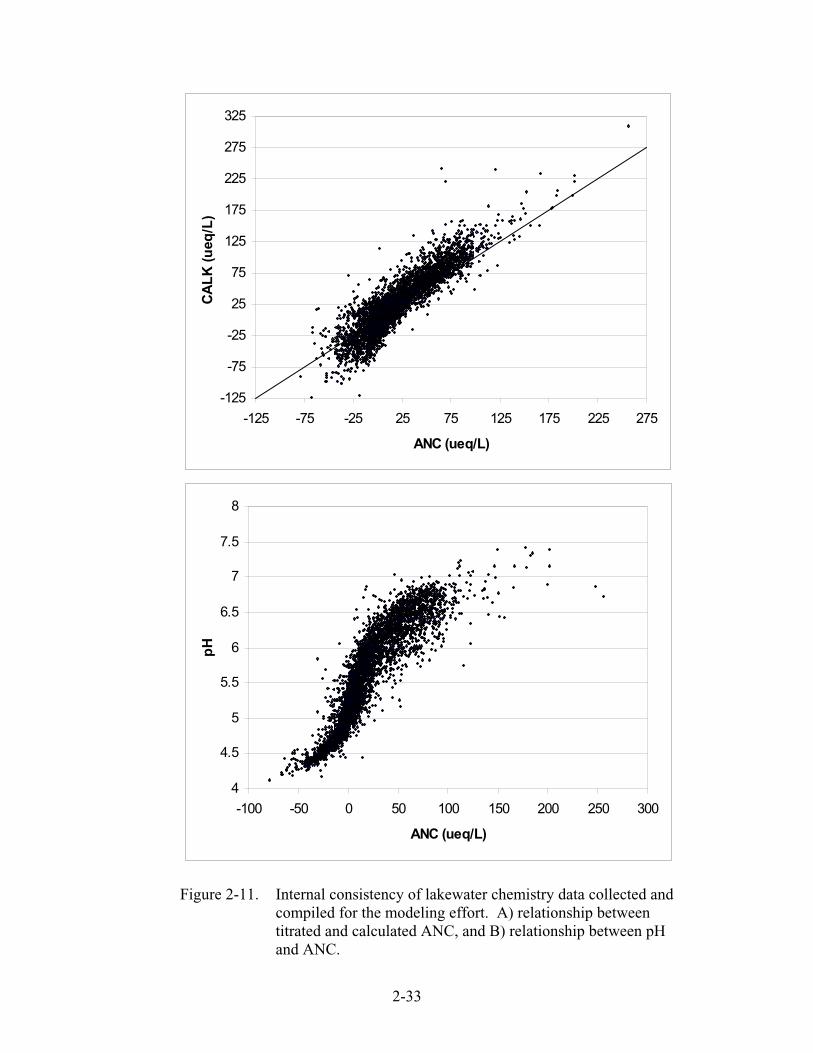
2-10 Relationships between a) titrated and calculated ANC and b) titrated ANC and pH for 13 lakewater samples collected in 2003 2-32
2-11 Internal consistency of lakewater chemistry data collected and compiled for the modeling effort 2-33
3-1 Regional soils types of the Adirondacks 3-4 3-2 Regional forest types of the Adirondacks 3-5 3-3 Locations of soil pits sampled for this study in the Adirondacks 3-6 3-4 Mapped landscape units and soil pit locations for one illustrative study
watershed (Rock Pond watershed) 3-7 35 Mean composition of the CECe and pHs from all watershed samples analyzed
in the Adirondack watershed sampling conducted in 2003 3-8 3-6 Soil base saturation for soil samples collected within the statistically-selected
EMAP study watersheds in the Adirondacks 3-9 3-7 Simulated versus observed average lakewater ANC (calculated from the charge
balance) and pH during the model calibrationevaluation period for each of the 70 study lakes 3-16
3-8 MAGIC simulations for the probability lakes that had ANC 20 eqL in 2000 under three scenarios of emissions controls 3-22
3-9 Cumulative distributions of PnET-BGC simulated water chemistry and soil base saturation for the population of Adirondack lakes (1320 lakes) in pre-industrial time (1850) 1980 and 2100 under three future emissions scenarios 3-23
3-10 PnET-BGC simulation results for the probability lakes that had ANC 20 eqL in 2000 under three scenarios of emissions controls 3-29
x
3-11 Percent base saturation of soils sampled from the B horizon of A) ALTM and AEAP watersheds and B) EMAP watersheds Base saturation is reported as percent frequency of occurrence within value ranges 3-30
3-12 CN molar ratio of O horizon and B horizon soil samples collected within the EMAP and ALTMAEAP study watersheds 3-31
3-13 MAGIC model simulated watershed B horizon soil percent base saturation from pre-industrial times to the year 2100 for two sets of study lakes the population represented by the EMAP lakes and the ALTMAEAP long-term monitoring lakes 3-32
3-14 PnET-BGC model simulated values of watershed B horizon soil percent base saturation from pre-industrial times (~1850) to the year 2100 for two sets of study lakes the population represented by the EMAP lakes and the ALTM AEAP long-term monitoring lakes 3-33
3-15 MAGIC model simulated lakewater sulfate concentration from pre-industrial times (~1850) to the year 2100 for two sets of study lakes the population represented by the EMAP lakes and the ALTMAEAP long-term monitoring lakes 3-36
3-16 PnET-BGC model simulated lakewater sulfate concentration from preshyindustrial times (~1850) to the year 2100 for two sets of study lakes the population represented by the EMAP lakes and the ALTMAEAP long-term monitoring lakes 3-36
3-17 MAGIC model simulated lakewater acid neutralizing capacity from preshyindustrial times to the year 2100 for two sets of study lakes the population represented by the EMAP lakes and the ALTMAEAP long-term monitoring lakes 3-37
3-18 PnET-BGC model simulated lakewater acid neutralizing capacity from preshyindustrial times (~1850) to the year 2100 for two sets of study lakes the population represented by the EMAP lakes and the ALTMAEAP long-term monitoring lakes 3-37
3-19 Fish species richness of Adirondack lakes as a function of ANC 3-43 3-20 Zooplankton taxonomic richness versus ANC for the combined Adirondack
dataset based on 111 lake visits to 97 lakes in the EMAP ELS and STAR zooplankton surveys 3-45
3-21 Cluster dendrogram of the three PCA axis scores 3-47 3-22 Factor axis plots showing separation of clusters 3-48 3-23 Top panel 2000 lakewater ANC and site source distribution across PCA axis
1-2 scores Bottom panel distribution of data points across datasets 3-52 4-1 Cumulative distribution functions of lakewater ANC at three periods for the
population of Adirondack lakes based on MAGIC model simulations 4-4 4-2 Cumulative distribution functions of lakewater ANC at three periods for the
population of Adirondack lakes based on PnET-BGC model simulations 4-4 4-3 MAGIC model projections of lakewater ANC (top panel) and watershed soil
base saturation (bottom panel) for the period 1950 to 2100 for all modeled lakes that had ANC in the year 2000 less than or equal to 20 eqL 4-5
4-4 PnET-BGC model projections of lakewater ANC (top panel) and watershed soil base saturation (bottom panel) for the period 1950 to 2100 for all modeled lakes that had ANC in the year 2000 less than or equal to 20 eqL 4-7
xi
4-5 Relationship between watershed-aggregated B-horizon soil percent base saturation and lakewater ANC for the 70 study lake watersheds 4-8
4-6 Correlations between total C and CECe from all soil samples analyzed in the Adirondack watershed sampling conducted in 2003 4-11
4-7 Correlations between total C in the soil and H+ in equilibrium soil solutions from the soil pH in water measurements 4-11
4-8 Cumulative distribution functions for a common population of Adirondack lake watersheds constructed for DDRP data collected in the mid 1980s and data compiled or collected in this study for EMAP lake watersheds in the early 1990s (lake chemistry) and in 2003 (soil chemistry) 4-14
49 Cumulative distribution functions of estimated total zooplankton species richness for the population of Adirondack lakes based on PnET-BGC model estimates of lakewater ANC and the empirical relationship between total zooplankton species richness and lakewater ANC in Adirondack lakes 4-16
410 Cumulative distribution functions of changes in estimated total zooplankton species richness for the population of Adirondack lakes based on PnET-BGC model estimates of lakewater ANC and the empirical relationship between total zooplankton species richness and ANC in Adirondack lakes 4-17
4-11 Cumulative distribution functions of the probability of fish species richness for hindcasts (a) and forecasts (b) for the EMAP population of Adirondack lakes using PnET-BGC 4-19
4-12 Cumulative distribution functions of the difference in probability of fish species richness between 1850 and 1990 between 1990 and 2100 for the Base Case scenario between 1990 and 2100 for the Moderate scenario and between 1990 and 2100 for the Aggressive scenario for the EMAP population of Adirondack lakes using PnET-BGC 4-21
4-13 Cumulative distribution functions of the probability of brook trout presence for hindcasts (a) and forecasts (b) for the EMAP population of Adirondack lakes using PnET-BGC 4-22
4-14 Cumulative distribution functions of the difference in the probability of brook trout presence between 1850 and 1990 between 1990 and 2100 for the Base Case scenario between 1990 and 2100 for the Moderate scenario and between 1990 and 2100 for the Aggressive scenario for the EMAP population of Adirondack lakes using PnET-BGC 4-23
4-15 Comparison of 1990 values simulated by PnET-BGC with averages of observed values for the period 1985-1994 for several variables 4-26
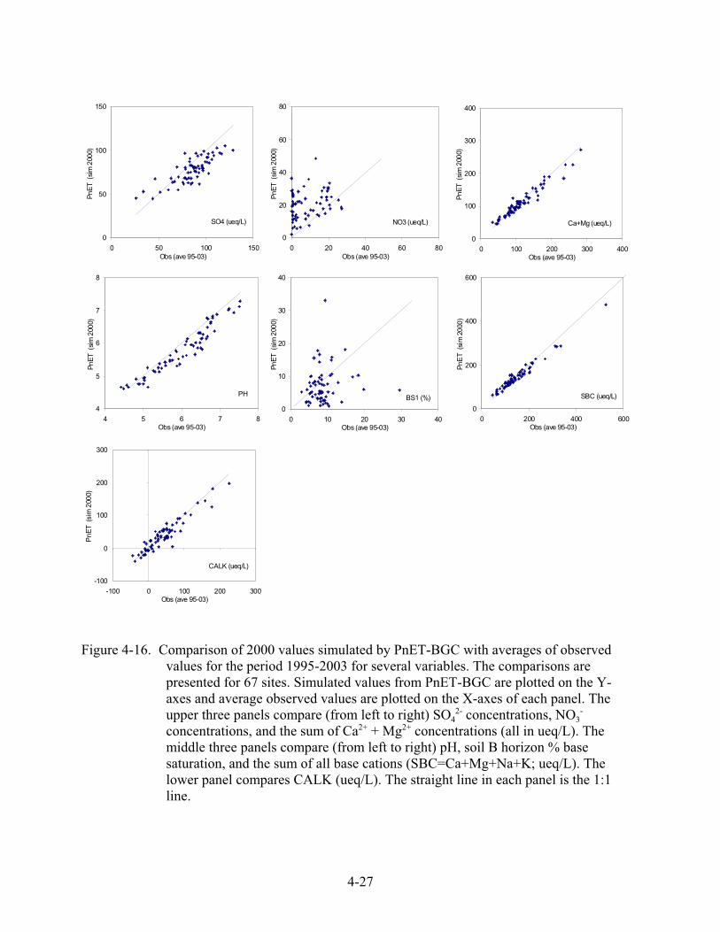
4-16 Comparison of 2000 values simulated by PnET-BGC with averages of observed values for the period 1995-2003 for several variables 4-27
4-17 Comparison of 1990 values simulated by MAGIC with averages of observed values for the period 1985-1994 for several variables 4-28
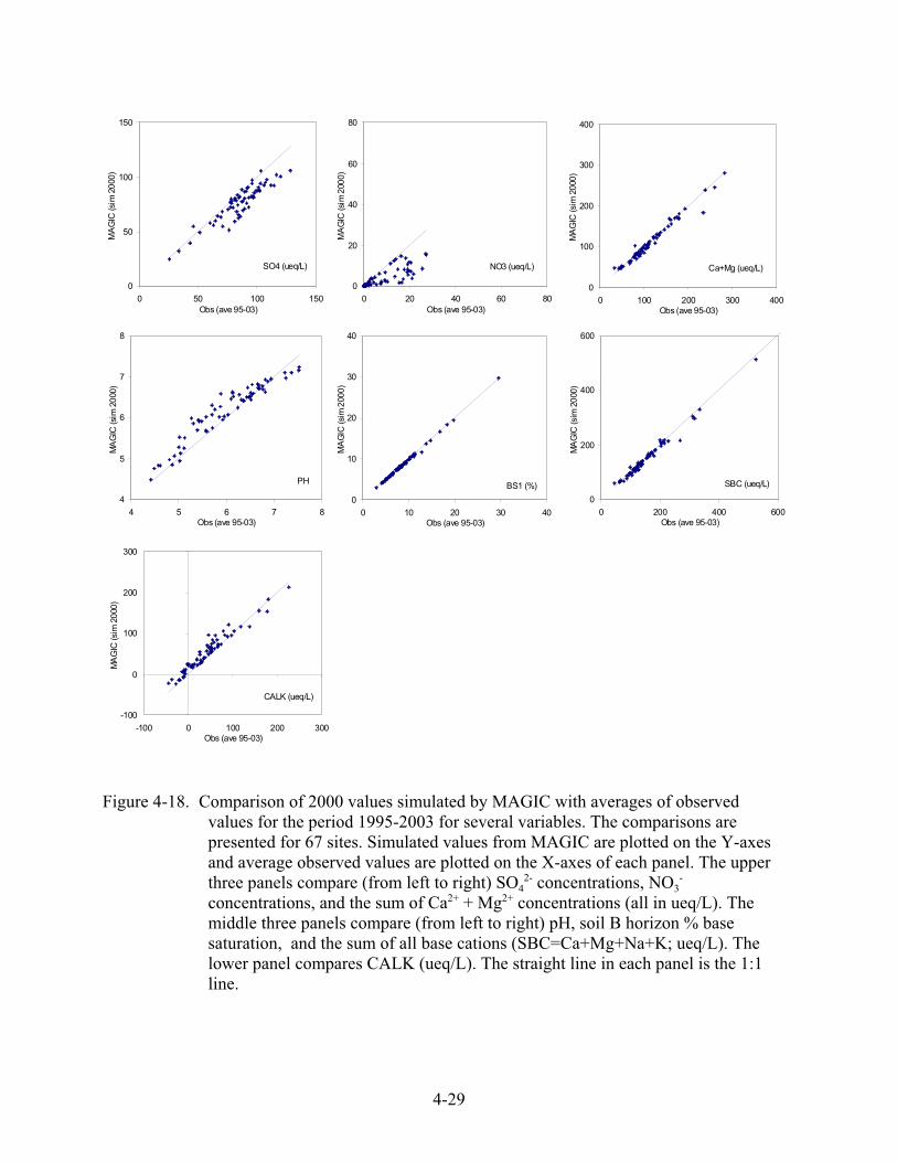
4-18 Comparison of 2000 values simulated by MAGIC with averages of observed values for the period 1995-2003 for several variables 4-29
4-19 Comparison of 1850 simulated values for several variables for the two models 4-30 4-20 Comparison of 1990 simulated values for several variables for the two models 4-32 4-21 Comparison of 2000 simulated values for several variables for the two models 4-33 4-22 Comparison of 2100 simulated values for several variables for the two models
for the base future deposition scenario 4-34
xii
4-23 Comparison of 2100 simulated values for several variables for the two models for the moderate future deposition scenario 4-35
4-24 Comparison of 2100 simulated values for several variables for the two models for the aggressive future deposition scenario 4-36
4-25 Cumulative distribution functions of selected major ions (eqL) calculated ANC of lakewater (eqL) and B-horizon soil base saturation for the MAGIC and PnET-BGC models 4-38
4-26 Cumulative distribution functions of selected major ions and calculated ANC of lakewater (eqL) and of B-horizon soil base saturation for the MAGIC and PnET-BGC models 4-40
4-27 Comparison of simulated values of CALK (ueqL) for the two models 4-41 4-28 Left Model estimates of historical change in CALK from 1850 to 1990 (negative
changes imply acidification since pre-industrial times) versus average estimated S deposition for 1990-2000 to the midpoint of each study watershed (MAGIC projections are given in upper left panel and PnET-BGC projections are given in lower left) Right Simulated changes in lakewater CALK from 1990 to 2100 under the Aggressive Additional Emissions Controls scenario versus average estimated S deposition for 1990-2000 to the midpoint of each study watershed 4-42
4-29 Left Model estimates of historical change in CALK from 1850 to 1990 (negative changes imply acidification) versus simulated CALK (average of 1990 and 2000 values) MAGIC projections are given in upper left panel and PnET-BGC projections are given in lower left Right Simulated changes in lakewater CALK from 1990 (approximate period of lowest CALK) to 2100 under the Aggressive Additional Emissions Controls scenario versus simulated CALK (average of 1990 and 2000 values) 4-43
4-30 Model estimates of change in CALK from 1990 to 2000 (negative changes imply continuing acidification) versus simulated CALK (average of 1990 and 2000) 4-45
4-31 Left Model estimates of historical change in CALK from 1850 to 1990 (negative changes imply acidification) versus simulated B-horizon soil BS (average of 1990 and 2000 values) MAGIC projections are given in upper left panel and PnET-BGC projections are given in lower left Right Simulated changes in lakewater CALK from 1990 (approximate period of lowest CALK) to 2100 under the Aggressive Additional Emissions Controls scenario versus simulated B-horizon soil BS (average of 1990 and 2000 values) 4-46
4-32 Cumulative distribution functions (CDF) of lakewater acid base chemistry and acidificationrecovery responses simulated with the MAGIC model for the population of Adirondack lakes having ANC 200 eqL 4-51
4-33 Box and whisker plots of lakewater ANC at three future points in time 2020 2050 and 2100 4-53
4-34 Box and whisker plots of lakewater SO4 2- concentration at three future points
in time 2020 2050 and 2100 4-53 4-35 Box and whisker plots of lakewater SO4
2- concentrations in pre-industrial and more recent times based on MAGIC model simulations under the Base Case emissions controls scenario 4-54
xiii
List of Tables
2-1 Study Watersheds 2-3 2-2 Analytical methods for lakewater chemistry used in this study 2-9 2-3 EPA emissions inventory (in million tons) for the Base Year (2001) 2-13 2-4 Future emissions in 2010 and 2015 of NOx SO2 and NH3 specified for the three
emissions control scenarios 2-15 2-5 Results of repeated (n=6) analyses throughout the duration of the field study
of aliquots from composite samples of organic and mineral soils representative of the study area 2-29
3-1 Number of sampled sites and median measured values of selected soil acid-base chemistry values for landscape types defined according to general forest type and general soil type 3-6
3-2 Population statistics for Adirondack soils based on a statistically-selected group of 44 potentially acid-sensitive Adirondack lake watersheds representative of 1320 lake watersheds with lakes larger than 1 ha that have acid neutralizing capacity less than 200 eqL 3-11
3-3 Mean and standard deviation of percent cation saturation values in O and B horizon soils by vegetation type 3-12
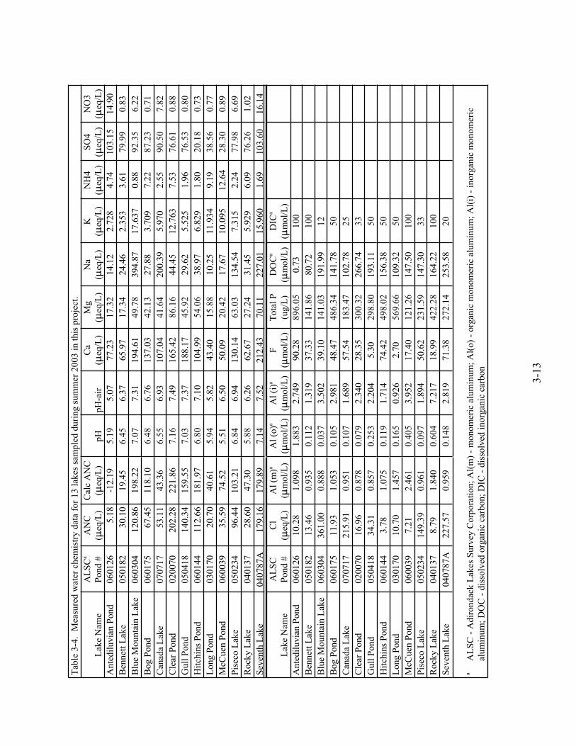
3-4 Measured water chemistry data for 13 lakes sampled during summer 2003 in this project 3-13
3-5 Average observed lakewater chemistry during the calibration period for each study lake 3-14
3-6 Simulated water chemistry percentile values for the population of potentially acid-sensitive Adirondack lakes based on the MAGIC model for the period from 1850 to 2100 assuming three scenarios of S and N emissions control 3-18
3-7 Estimated number of Adirondack lakes below ANC criteria values for the population of 1320 Adirondack lakes larger than 1 ha that have ANC less than 200 eqL based on MAGIC model simulations for 44 statistically-selected lakes 3-20
3-8 Estimated number of Adirondack lakes below pH criteria values for the population of 1320 Adirondack lakes larger than 1 ha that have ANC less than 200 eqL based on MAGIC model simulations for 44 statistically-selected lakes 3-21
3-9 Simulated water chemistry percentile values of annual concentrations for the population of potentially acid-sensitive Adirondack lakes based on the PnET-BGC model for the period from 1850 to 2100 assuming three scenarios of S and N emissions control (Units eqL except pH) 3-25
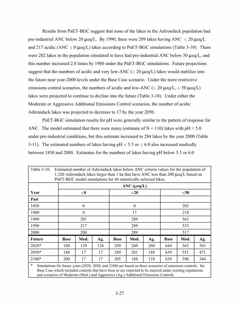
3-10 Estimated number of Adirondack lakes below ANC criteria values for the population of 1320 Adirondack lakes larger than 1 ha that have ANC less than 200 eqL based on PnET-BGC model simulations for 44 statistically-selected lakes 3-27
3-11 Estimated number of Adirondack lakes below pH criteria values for the population of 1320 Adirondack lakes larger than 1 ha that have ANC less than 200 eqL based on PnET-BGC model simulations for 44 statistically-selected lakes 3-28
xiv
3-12 Relationship between each of the long-term monitoring study watersheds and the EMAP population of Adirondack lake watersheds with respect to modeled soil base status based on the MAGIC model 3-35
3-13 Summary of the sensitivity of PnET-BGC model output of lakewater acid neutralizing capacity (SANC) and B horizon soil base saturation (S BS) to selected model parameters 3-41
3-14 Observed relationships between zooplankton species richness (R) and lakewater ANC 3-44
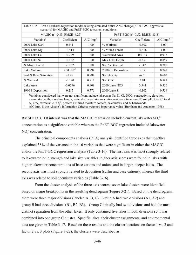
3-15 Best all-subsets regression model relating future ANC change (2100-1990 aggressive scenario) for MAGIC and PnET-BGC to current conditions 3-46
3-16 Principal components analysis pattern showing correlations of variables with top three factor components 3-47
3-17 List of lakes and their characteristics by cluster ID 3-49 3-18 Number of lakes in PCA clusters 3-51 4-1 MAGIC model projections of acidification and recovery (change in lakewater
acid-base chemistry) for the population of potentially acid-sensitive Adirondack lakes based on estimates of historical emissions and three scenarios of future emissions controls 4-3
4-2 PnET-BGC model projections of acidification and recovery (change in lakewater acid-base chemistry) for the population of potentially acid-sensitive Adirondack lakes based on estimates of historical emissions and three scenarios of future emissions controls 4-3
4-3 Modeled relationship between each of the studied ALTMAEAP lakes and the population of Adirondack lakes with respect to acid-base chemistry status acidification and recovery responses based on MAGIC model simulations 4-48
4-4 Modeled relationship between each of the studied ALTMAEAP lakes and the population of Adirondack lakes with respect to acid-base chemistry status acidification and recovery responses based on PnET-BGC model simulations 4-49
xv
List of Acronyms
AEAP Aquatic Effects Assessment Program
AIC Aikakersquos Information Criteria
AirMon Atmospheric Integrated Research Monitoring Network
ALSC Adirondack Lakes Survey Corporation
ALTM Adirondack Long-term Monitoring Program
ANC Acid neutralizing capacity
BS Base saturation
CAIR Clean Air Interstate Rule
CALK Calculated ANC
CASTNet Clean Air Status and Trends Network
CEC Cation exchange capacity
CEC e Effection cation exchange capacity
DDRP Direct Delayed Response Project
DIC Dissolved inorganic carbon
DOC Dissolved organic carbon
EGU Electricity generating units
ELS Eastern Lake Survey
ELS-II Phase II of the Eastern Lake Survey
EMAP Environmental Monitoring and Assessment Program
EPA Environmental Protection Agency
GIS Geographic information system
GPS global positioning system
HDDE Heavy duty diesel engines
IAQR Interstate Air Quality Rule
LNDE Land-based non-road diesel engines
LOI Loss on ignition
LTM Long-term Monitoring program
MACT Maximum achievable control technology
MAGIC Model of Acidification of Groundwater in Catchments
NADP National Atmospheric Deposition Program
NAPAP National Acid Precipitation Assessment Program
NY-GAP New York State Gap Analysis Program
NYSDEC New York State Department of Environmental Conservation
NYSERDA New York State Energy Research and Development Authority
PCA Principal components analysis
PM Particulate matter
PnET-BGC Photosynthesis and evapotranspiration biogeochemistry model
QAQC Quality assuranceQuality Control
RACT Reasonably available control technology
RMSE Root mean square error
SAA Sum of acid anions
SBC Sum of base cations
SIP State Implementation Plan
STAR Science to Achieve Results
USDA US Department of Agriculture
UV-B Ultraviolet radiation
xvi
Glossary
Acid anion - negatively charged ion that does not react with hydrogen ion in the pH range of
most natural waters
Acid-base chemistry - the reaction of acids (proton donors) with bases (proton acceptors) In
the context of this report this means the reactions of natural and anthropogenic acids and bases
the result of which is described in terms of pH and acid neutralizing capacity of the system
Acid cation - hydrogen ion or metal ion that can hydrolyze water to produce hydrogen ions eg
ionic forms of aluminum manganese and iron
Acid neutralizing capacity (ANC) - the equivalent capacity of a solution to neutralize strong
acids The components of ANC include weak bases (carbonate species dissociated organic
acids alumino-hydroxides borates and silicates) and strong bases (primarily OH -) ANC can be
measured in the laboratory by the Gran titration procedure or defined as the difference in the
equivalent concentrations of the base cations and the mineral acid anions
Acidic deposition - transfer of acids and acidifying compounds from the atmosphere to
terrestrial and aquatic environments via rain snow sleet hail cloud droplets particles and gas
exchange
Acidic episode - an episode in a water body in which acidification of surface water to an acid
neutralizing capacity less than or equal to 0 occurs
Acidic lake or stream - a lake or stream in which the acid neutralizing capacity is less than or
equal to 0
Acidification - the decrease of acid neutralizing capacity in water or base saturation in soil
caused by natural or anthropogenic processes
Acidified - pertaining to a natural water that has experienced a decrease in acid neutralizing
capacity or a soil that has experienced a reduction in base saturation
Acidophilic - describing organisms that thrive in an acidic environment
Analyte - a chemical species that is measured in a water sample
Anion - a negatively charged ion
Anthropogenic - of relating to derived from or caused by humans or related to human
activities or actions
Base cation - an alkali or alkaline earth metal cation (Ca2+ Mg2+ K+ Na+)
xvii
Base cation buffering - the capacity of a watershed soil or a sediment to supply base cations
(Ca2+ Mg2+ K+ Na+) to receiving surface waters in exchange for acid cations (H+ Al3+) may
occur through cation exchange in soils or weathering of soil or bedrock minerals
Base cation supply - The rate at which base cations can be supplied to buffer incoming acid
cations this rate is determined by the relative rate of mineral weathering the availability of base
cations on exchange sites and the rate of mobile anion leaching
Base saturation - the proportion of total soil cation exchange capacity that is occupied by
exchangeable base cations ie by Ca2+ Mg2+ K+ and Na+
Bias - a systematic difference (error) between a measured (or predicted) value and its true value
Biological effects - changes in biological (organismal populational community-level) structure
andor function in response to some causal agent also referred to as biological response
Calibration - process of checking adjusting or standardizing operating characteristics of
instruments or coefficients in a mathematical model with empirical data of known quality The
process of evaluating the scale readings of an instrument with a known standard in terms of the
physical quantity to be measured
Catchment - see watershed
Cation - a positively charged ion
Cation exchange - the interchange between a cation in solution and another cation on the surface
of any surface-active material such as clay or organic matter
Cation exchange capacity - the sum total of exchangeable cations that a soil can adsorb
Cation leaching - movement of cations out of soil in conjunction with mobile anions in soil
solution
Cation retention - the physical biological and geochemical processes by which cations in
watersheds are held retained or prevented from reaching receiving surface waters
Chronic acidification - see long-term acidification
Circumneutral - close to neutrality with respect to pH (neutral pH = 7) in natural waters pH 6shy
8
Conductance - (See specific conductance)
Confidence limits - a statistical expression based on a specified probability that estimates the
upper andor lower value (limit) or the interval expected to contain the true population mean
xviii
Decomposition - the microbially mediated reaction that converts solid or dissolved organic
matter into its constituents (also called decay or mineralization)
Denitrification - biologically mediated conversion of nitrate to gaseous forms of nitrogen (N2
NO N2O) denitrification occurs during decomposition of organic matter
Dissolved inorganic carbon - the sum of dissolved (measured after filtration) carbonic acid
bicarbonate and carbonate in a water sample
Dissolved organic carbon - organic carbon that is dissolved or unfilterable in a water sample
(045-jm pore size)
Drainage basin - see watershed
Drainage lake - a lake that has a permanent surface water inlet and outlet
Dry deposition - transfer of substances from the atmosphere to terrestrial and aquatic
environments via gravitational settling of large particles and turbulent transfer of trace gases and
small particles
Dynamic model - a mathematical model in which time is included as an independent variable
Empirical model - representation of a real system by a mathematical description based on
experimental or observational data
Episodes - a subset of hydrological phenomena known as events Episodes driven by rainfall or
snowmelt occur when acidification takes place during a hydrologic event Changes in other
chemical parameters such as aluminum and calcium are frequently associated with episodes
Episodic acidification - the short-term decrease of acid neutralizing capacity from a lake or
stream This process has a time scale of hours to weeks and is usually associated with
hydrological events
Equivalent - unit of ionic concentration a mole of charge the quantity of a substance that either
gains or loses one mole of protons or electrons
Evapotranspiration - the process by which water is returned to the air through direct
evaporation or transpiration by vegetation
Forecast - to estimate the probability of some future event or condition as a result of rational
study and analysis of available data
Frame - a structural representation of a population providing a sampling capability
Gran analysis - a mathematical procedure used to determine the equivalence points of a titration
curve for acid neutralizing capacity
xix
Ground water - water in a saturated zone within soil or rock
Hindcast - to estimate the probability of some past event or condition as a result of rational study
and analysis of available data
Hydraulic residence time - a measure of the average amount of time water is retained in a lake
basin It can be defined on the basis of inflowlake volume represented as RT or on the basis
of outflow (outflowlake volume) and represented as TW The two definitions yield similar
values for fast-flushing lakes but diverge substantially for long-residence time seepage lakes
Hydrologic(al) event - pertaining to increased water flow or discharge resulting from rainfall or
snowmelt
Hydrologic(al) flow paths - surface and subsurface routes by which water travels from where it
is deposited by precipitation to where it drains from a watershed
Hydrology - the science that treats the waters of the earth--their occurrence circulation and
distribution their chemical and physical properties and their reaction with their environment
including their relationship to living things
Inorganic aluminum - the sum of free aluminum ions (Al3+) and dissolved aluminum bound to
inorganic ligands operationally defined by labile monomeric aluminum
Labile monomeric aluminum - operationally defined as aluminum that can be retained on a
cation exchange column and measured by one of the two extraction procedures used to measure
monomeric aluminum Labile monomeric aluminum is assumed to represent inorganic
monomeric aluminum (Ali)
Liming - the addition of any base materials to neutralize surface water or sediment or to increase
acid neutralizing capacity
Littoral zone - the shallow near-shore region of a body of water often defined as the band from
the shoreline to the outer edge of the occurrence of rooted vegetation
Long-term acidification - the decrease of acid neutralizing capacity in a lake or stream over a
period of hundreds to thousands of years generally in response to gradual leaching of ionic
constituents
Mineral acids - inorganic acids eg H2SO4 HNO3 HCl H2CO3
Mineralization - process of converting organic nitrogen in the soil into ammonium which is
then available for biological uptake
Mineral weathering - dissolution of rocks and minerals by chemical and physical processes
Mitigation - generally described as amelioration of adverse impacts caused by acidic deposition
at the source (eg emissions reductions) or the receptor (eg lake liming)
xx
Mobile anions - anions that flow in solutions through watershed soils wetlands streams or
lakes without being adsorbed or retained through physical biological or geochemical processes
Model - an abstraction or representation of a prototype or system generally on a smaller scale
Monomeric aluminum - aluminum that occurs as a free ion (Al3+) simple inorganic complexes 3-n 3-n(eg Al(OH)n AlFn ) or simple organic complexes but not in polymeric forms
operationally extractable aluminum measured by the pyrocatechol violet method or the methylshy
isobutyl ketone method (also referred to as the oxine method) is assumed to represent total
monomeric aluminum Monomeric aluminum can be divided into labile and non-labile
components using cation exchange columns
Monte Carlo method - technique of stochastic sampling or selection of random numbers to
generate synthetic data
Natural acids - acids produced within terrestrial or aquatic systems through natural biological
and geochemical processes ie not a result of acidic deposition or deposition of acid precursors
Nitrification - oxidation of ammonium to nitrite or nitrate by microorganisms A by-product of
this reaction is H+
Nitrogen fixation - biological conversion of elemental nitrogen (N2) to organic N
Nitrogen saturation - condition whereby nitrogen inputs to an alpine or forested ecosystem
exceed plant uptake requirements
Non-labile monomeric aluminum - operationally defined as aluminum that passes through a
cation exchange column and is measured by one of the two extraction procedures used to
measure monomeric aluminum assumed to represent organic monomeric aluminum (Alo)
Organic acids - heterogeneous group of acids generally possessing a carboxyl (-COOH) group
or phenolic (C-OH) group includes fulvic and humic acids
Organic aluminum - aluminum bound to organic matter operationally defined as that fraction
of aluminum determined by colorimetry after sample is passed through a strong cation exchange
column
Parameter - (1) a characteristic factor that remains at a constant value during the analysis or
(2) a quantity that describes a statistical population attribute
pH - the negative logarithm of the hydrogen ion activity The pH scale is generally presented
from 1 (most acidic) to 14 (most alkaline) a difference of one pH unit indicates a tenfold change
in hydrogen ion activity
Physiography - the study of the genesis and evolution of land forms a description of the
elevation slope and aspect of a study area
Plankton - plant or animal species that spend part or all of their lives in open water
xxi
Pool - in ecological systems the supply of an element or compound such as exchangeable or
weatherable cations or adsorbed sulfate in a defined component of the ecosystem
Population - for the purpose of this report (1) the total number of lakes within a given
geographical region or the total number of lakes with a given set of defined chemical physical
or biological characteristics or (2) an assemblage of organisms of the same species inhabiting a
given ecosystem
Precision - a measure of the capacity of a method to provide reproducible measurements of a
particular analyte (often represented by variance)
Probability sample - a sample in which each unit has a known probability of being selected
Project - to estimate future possibilities based on rational study and current conditions or trends
Quality assurance - a system of activities for which the purpose is to provide assurance that a
product (eg data base) meets a defined standard of quality with a stated level of confidence
Quality control - steps taken during sample collection and analysis to ensure that data quality
meets the minimum standards established in a quality assurance plan
Regionalization - describing or estimating a characteristic of interest on a regional basis
Retention time - the estimated mean time (usually expressed in years) that water resides in a
lake prior to leaving the system (See hydraulic residence time)
Scenario - one possible deposition sequence following implementation of a control or
mitigation strategy and the subsequent effects associated with this deposition sequence
Short-term acidification - see episode
Simulation - description of a prototype or system response to different conditions or inputs
using a model rather than actually observing the response to the conditions or inputs
Simulation model - mathematical model that is used with actual or synthetic input data or
both to produce long-term time series or predictions
Species richness - the number of species occurring in a given aquatic ecosystem generally
estimated by the number of species caught using a standard sampling regime
Specific conductance - the conductivity between two plates with an area of 1 cm2 across a
distance of 1 cm at 25degC
Steady state - the condition that occurs when the sources and sinks of a property (eg mass
volume concentration) of a system are in balance (eg inputs equal outputs production equals
consumption)
xxii
Stratified design - a statistical design in which the population is divided into strata and a
sample selected from each stratum
Strong acid anion sum (SAA or CA) - refers to the equivalent sum of SO42- NO3
- Cl- and F -
The term specifically excludes organic acid anions
Strong acids - acids with a high tendency to donate protons or to completely dissociate in natural
waters eg H2SO4 HNO3 HCl- and some organic acids (See acid anions)
Strong bases - bases with a high tendency to accept protons or to completely dissociate in
natural waters eg NaOH
Subpopulation - any defined subset of the target population
Sulfate adsorption - the process by which sulfate is chemically exchanged (eg for OH -) or
adsorbed onto positively charged sites on the soil matrix under some conditions this process is
reversible and the sulfate may be desorbed
Sulfate reduction - (1) the conversion of sulfate to sulfide during the decomposition of organic
matter under anaerobic conditions (dissimilatory sulfate reduction) and (2) the formation of
organic compounds containing reduced sulfur compounds (assimilatory sulfate reduction)
Sulfate retention - the physical biological and geochemical processes by which sulfate in
watersheds is held retained or prevented from reaching receiving surface waters
Sum of base cations (SBC or CB) - refers to the equivalent sum of Ca2+ Mg2+ Na+ and K+ The
term specifically excludes cationic Aln+ and Mn2+
Surficial geology - characteristics of the earths surface especially consisting of unconsolidated
residual colluvial alluvial or glacial deposits lying on the bedrock
Target population - a subset of a population explicitly defined by a given set of exclusion
criteria to which inferences are to be drawn from the sample attributes
Total monomeric aluminum - operationally defined simple unpolymerized form of aluminum
present in inorganic or organic complexes
Turnover - the interval of time in which the density stratification of a lake is disrupted by
seasonal temperature variation resulting in entire water mass becoming mixed
Variable - a quantity that may assume any one of a set of values during analysis
Watershed - the geographic area from which surface water drains into a particular lake or point
along a stream
Weak acids - acids with a low proton-donating tendency that tend to dissociate only partially in
natural waters eg H2CO3 H4SiO4 and most organic acids (See acid anions)
xxiii
Weak bases - bases with a low proton-accepting tendency that tend to dissociate only partially in
natural waters eg HCO3- Al(OH)4
-
Wet deposition - transfer of substances from the atmosphere to terrestrial and aquatic
environments via precipitation eg rain snow sleet hail and cloud droplets Droplet
deposition is sometimes referred to as occult deposition
xxiv
10 INTRODUCTION
Ecosystem damage from air pollution in the Adirondack Mountains New York is
believed to have been substantial mainly from atmospheric deposition of sulfur (S Driscoll et
al 1991 Sullivan 2000 Driscoll et al 2003) Most efforts to quantify damages and to examine
more recent ecosystem recovery have focused on lakewater chemistry However relatively
large decreases in regional upwind S emissions and generally similar decreases in S deposition
in the Adirondack Mountains over the past two decades have resulted in limited recovery of 2-)lakewater acid-base chemistry (Stoddard et al 1998 2003 Driscoll et al 2003) Sulfate (SO4
concentrations in lakewater have decreased markedly but so have the concentrations of base
cations Therefore measured increases in lakewater pH and acid neutralizing capacity (ANC)
have generally been small This limited chemical recovery of surface waters in the Adirondack
Mountains and elsewhere in the northeastern United States has been attributed in large part to
base cation depletion especially Ca2+ of watershed soils (Lawrence et al 1995 Likens et al
1996) in response to long-term elevated levels of S deposition Changes in atmospheric
deposition of base cations have also likely contributed (Gbondo-Tugbawa and Driscoll 2003)
The relatively small recent increases in lakewater pH and ANC in response to substantial
reductions (gt 40) in S deposition (Stoddard et al 2003) might be attributable to remaining
base cation exchange buffering in these watershed soils There is evidence that historic increases
in S deposition resulted in large increases in base cation concentrations of many Adirondack
lakes resulting in only small reductions in ANC during that period (cf Sullivan et al 1990
Cumming et al 1992) Thus it might be reasonable to expect that subsequent decreases in
solution SO42- concentrations and mobility would result in decreased base cation concentrations
in runoff Unfortunately data that characterize the acid-base chemistry of Adirondack soils are
scarce particularly data that define changes in soil conditions over time
Much of the acidic deposition effects research in the Adirondacks has focused on
individual lakes and their watersheds There is a great deal of information available for a
relatively small number of watersheds (cf Driscoll et al 1991 Sullivan 2000) including
intensive chemical and in many cases biological monitoring data collected during the past one
to two decades Despite substantial variability there are recognizable patterns with respect to
watershed characteristics associated with various acidification processes (cf Driscoll and
Newton 1985 Driscoll et al 1991 Sullivan et al 1999) However knowledge of acidification
and recovery processes for individual watersheds is of limited value as a basis for public policy
1-1
It is necessary to determine the extent to which these well-studied watersheds represent larger
units Management decisions require information regarding numbers and percentages of lakes
that have behaved or in the future will be expected to behave in various ways Clearly
chemical and likely biological recovery is now occurring in some Adirondack lakes We need
to know how many what kind and the extent to which such recovery will continue andor
accelerate in response to current or further decreased S and nitrogen (N) deposition
Databases developed by six major research programs offer an opportunity to evaluate the
chronic effects of acidic deposition on acid-sensitive Adirondack watersheds the Eastern Lakes
Survey (ELS Linthurst et al 1986) DirectDelayed Response Project (DDRP) (Church et al
1989) Environmental Monitoring and Assessment Program (EMAP Larsen et al 1994)
Adirondack Long-Term Monitoring Project (ALTM Driscoll et al 2003a) Adirondack Effects
Assessment Program (AEAP) and the Adirondack Lakes Survey Corporations (ALSC) survey
(Kretser et al 1989) The ELS DDRP and EMAP studies were all statistically based thereby
allowing population estimates to be developed ALTM and AEAP involve on-going long-term
lake monitoring efforts but are not statistically based Only DDRP contained a soils sampling
component but the soils data were aggregated to the entire northeastern United States rather
than the Adirondack Mountain region
Long-term monitoring programs have been collecting chemical and biological data for
the past one to two decades from Adirondack lakes some of which show evidence of recent
resource recovery The ALTM project has been conducting monthly monitoring of the water
chemistry of 17 lakes mostly in the southwestern Adirondack Mountains since 1982 (Driscoll et
al 2003) In 1992 the program was expanded by the addition of 35 lakes to the monitoring
effort The AEAP has been sampling the water chemistry zooplankton and fisheries of 30 lakes
approximately twice per summer since 1994 Most of those lakes are also included within
ALTM Because the ALTM and AEAP study lakes were not statistically selected they can be
considered judgment samples
The most extensive survey of lakewater chemistry in the Adirondack Mountains was that
of the ALSC (Kretser et al 1989 Baker et al 1990) Over a four-year period ALSC surveyed
the chemistry and fisheries of 1469 lakes Despite the large number of lakes included however
they were not drawn from a statistical frame and therefore the results cannot be used for
population estimates
1-2
The best statistical frame for assessing acidification and recovery responses of
Adirondack lakes was developed by the US EPAs EMAP (Larsen et al 1994) The EMAP
included lakes as small as 1 ha involved both chemical and more limited biological
characterization and it was based on more accurate maps than the DDRP The EMAP was
designed to provide unbiased regional characterization of the entire population of Adirondack
Mountain lakes
There is currently not a mechanism available with which to extrapolate results of either
of the chemical and long-term biological monitoring studies to the regional population of
Adirondack lakes and this seriously curtails the ultimate utility of these important data
Resource managers and policymakers need to know the extent to which current and projected
future emissions reductions will lead to regional ecosystem recovery both chemical and
biological Such recovery is being quantified at the ALTM and AEAP monitoring site locations
but could not be directly extrapolated to the larger population of lakes in the region The ALTM
and AEAP were designed to study lake-specific trends and seasonality The focus has mainly
been on lakes that are highly responsive to changes in acidic deposition Site selection for the
ALTM and AEAP programs was driven in part by such considerations as the existence of
historical andor ongoing data collection sampling logistics and the expectation that lakes in the
southwestern portion of the Adirondack Mountains region had been most impacted by acidic
deposition Questions of representativeness of the study lakes as compared with the region were
not considered
Stoddard et al (1998) found that long-term monitoring (LTM) sites in the northeastern
US including those in the Adirondacks covered the range of current ANC and base cation
concentrations of the most sensitive subpopulations of lakes in the Northeast region Thus the
intensive monitoring studies and EMAP apparently do not represent the same population of
lakes Information has not been available with which to determine the extent to which these
generally low-ANC ALTM lakes are representative of the overall population with respect to
acidification and recovery responses
Rates of ongoing and future ANC increase in Adirondack lakes in response to decreases
in acidic deposition are of considerable policy interest However making regional assessments
from sites such as the long-term monitoring sites that were not statistically selected can lead to
incorrect evaluations Paulsen et al (1998) reported on a number of inaccurate assessments
made as a result of extrapolating such data In all cases a statistically-based probability survey
1-3
showed markedly different regional conditions than did an evaluation that assumed that available
data adequately represented the regional population of interest The data record for the EMAP
probability lakes is insufficient for measurement of recovery responses Although these lakes
can be used as a basis for model forecasts of recovery they provide limited ability to determine
whether or not predicted responses actually occur Similarly the scarcity of seasonal water
chemistry data and biological response data for the probability lakes limit their utility for
assessment purposes Nevertheless the probability lakes are essential in order to place results
and conclusions from the intensively-monitored lakes into the regional context
Future changes in the structure and function of aquatic communities will be required to
restore ecosystem health Biological response data especially for zooplankton and to a lesser
extent for fish phytoplankton and bacteria are available for Adirondack lakes from the AEAP
EMAP ALTM and ALSC programs Data recently collected within these programs can provide
important information regarding the biological resources at greatest risk of adverse impacts from
acidic deposition and the spatial and temporal patterns of biological recovery as deposition
continues to decline
There is great interest in techniques such as liming to accelerate the recovery of aquatic
and terrestrial organisms in acid-sensitive regions of New York as acidic deposition continues to
be reduced If the rate of chemical recovery can be increased it may be possible to more rapidly
restore biological community structure and function However much can be gained by
examining the rate at which aquatic ecosystems are recovering now in response to recent
emissions reductions and to forecast the rate of near-term future recovery under already
promulgated air pollution controls Knowledge of the rate of ongoing responses and of the
characteristics associated with those lakes that are actually recovering is critical to development
of sound management policies Such information will provide the basis for evaluating the
efficacy of current and possibly expanded accelerated-recovery programs
Prior to initiation of this study there were no soil chemistry data available for most of the
EMAP watersheds in the Adirondack Mountains Furthermore there were no soil databases for
the Adirondack Mountain region that were well-suited for evaluating the effects of acidic
deposition on soils or for providing the basis for model projections of aquatic and terrestrial
resource recovery This critical data deficiency regarding Adirondack soils also precluded
effective and comprehensive regional modeling to (a) predict future responses of Adirondack
watersheds to varying emissions control scenarios (b) determine critical loads of atmospheric
1-4
deposition required to protect against further acidification or (c) define atmospheric deposition
goals to allow resource recovery
The US Environmental Protection Agencys (EPA) DDRP database (Church et al 1989)
has been used for several past modeling studies to project the response of Adirondack lakes to
varying scenarios of future acidic deposition (eg NAPAP 1991 Turner et al 1992 Van Sickle
and Church 1995) However there are several limitations of the DDRP soils database for
conducting an assessment of the responses of Adirondack lakes to various atmospheric
deposition scenarios today because
1 Soil aggregation for the DDRP was based on mapped soils information for the entire Northeast rather than the Adirondack sub-region specifically (a consequence of the broader regional objectives of the DDRP study) As a result soil data for a particular Adirondack watershed were not necessarily derived from soil pits actually excavated within that watershed or even within the Adirondack sub-region
2 The data are about two decades old and may not be compatible with data collected for current assessment purposes including data for intensively-studied watersheds
3 Although the DDRP watersheds were statistically selected they are representative only of watersheds containing lakes larger than 4 ha (a consequence of the regional maps available for Eastern Lakes Survey lake selection in 1985) It has subsequently been shown that a high proportion of smaller Adirondack lakes (1-4 ha) are acidic or highly acid-sensitive (Kretser et al 1989 Baker et al 1990 Sullivan 1990 Sullivan et al 1990) but were not included in the DDRP design
The degree to which regional Adirondack soil conditions exert controls on drainage water
chemistry is not well understood but may be substantial For example recent research in
Shenandoah National Park Virginia has shown a consistent pattern of lower streamwater ANC
in watersheds (n=14) having lower soil base saturation (BS) All Shenandoah watersheds that
had BS lt 15 also had average streamwater ANC lt 100 eqL None of the watersheds that
had ANC lt 20 eqL showed BS greater than about 12 (Sullivan et al 2003)
Here we integrate existing data from the AEAP ALTM EMAP and ALSC programs to
more fully utilize available data and provide the foundation for statistically representative
assessments of watershed responses to changing levels of S and N deposition The primary
objective was to develop an approach for extrapolating spatially-limited but temporally-intensive
knowledge regarding changes in the chemistry and biology of acid-sensitive lakes and their
1-5
watersheds in order to conduct regional assessments of ecosystem condition in the Adirondacks
In the process lakes were classified according to their responsiveness to future changes in S and
N deposition This research also developed a mechanism for further utilization of critical
biological response data that are available for a relatively small number of lakes
This research was undertaken to provide the foundation for determining the extent to
which impacted Adirondack lakes and their watershed soils can and will recover both
chemically and biologically following reductions in acidic deposition The focus is on the
Adirondack Mountain region as a whole and in particular the intensively-monitored watersheds
many of which are in the southwestern portion of Adirondack Park The latter group of
watersheds include many that contain shallow surficial deposits (thin-till) that are highly acid-
sensitive and that have been expected to be most responsive to reductions in acidic deposition
Our primary objective was to develop approaches for extrapolating spatially-limited
knowledge regarding changes in the chemistry and biology of acid-sensitive lakes and their
watersheds in order to conduct regional assessments of ecosystem condition and recovery in the
Adirondacks Secondary objectives included to develop a statistically-representative soils
database provide a mechanism for further utilization of critical biological response data that are
available for a relatively small number of lakes classify lakes according to their responsiveness
to future changes in S andor N deposition and provide the technical foundation for
establishment of critical and target loads of acid deposition An additional aim was to obtain a
clear picture of the temporal and spatial evolution of chemical and biological recovery processes
as lakes improve in acid-base chemistry in response to reductions in acidic deposition
1-6
20 METHODS
21 Site Selection
211 Study Watersheds
A group of watersheds was selected for soil sampling based on the EMAP statistical
design An additional set of watersheds was selected for sampling from among those that are
subjects of long-term chemical and biological monitoring efforts In the Adirondacks the
regional EMAP probability sample consisted of 115 lakes and their watersheds The total
number of target Adirondack lakes included in the EMAP frame was 1829 (SE = 244) These
include the lakes depicted on 1100000-scale USGS maps that were larger than 1 ha deeper
than 1 m and that contained more than 1000 m2 of open water Of those target lakes an
estimated 509 had summer index lakewater ANC gt 200 eqL these were considered insensitive
to acidic deposition effects and were not included in the study reported here The remaining
1320 (SE = 102) low-ANC lakes constituted the frame for extrapolation of soil results An
estimated 58 of these low-ANC target lakes had ANC lt 50 eqL at the time of EMAP
sampling (1991-1994) Details of the EMAP design were given by Larsen et al (1994)
Whittier et al (2002) presented an overall assessment of the relative effects of various
environmental stressors across northeastern lakes using EMAP probability survey data Based
on field measurements 42 of the lakes in the EMAP statistical frame had summer index ANC
50 eqL and another 30 had ANC between 50 and 200 eqL We focused this study on
watersheds containing these two strata of low ANC lakes ( 50 and between 50 and 200 eqL)
as they are thought to be most responsive to changes in air pollution Lakewater ANC provides
an integrating watershed acid-base chemistry variable that reflects biotic edaphic geologic and
hydrologic conditions from throughout the watershed Throughout this report we present
summer index ANC values These approximately correspond to annual average values ANC
measurements during spring especially in conjunction with snowmelt would be expected to be
lower
We used a random selection process to choose candidate watersheds for soil sampling
from among the 44 EMAP watersheds containing lakes with ANC 50 eqL and the 39 EMAP
watersheds containing lakes with ANC between 50 and 200 eqL Both primary and alternate
sampling candidates were selected in the order they were to be included in anticipation of the
problem that we would be unable to sample some of the selected watersheds (eg access
difficulty or permission denied) The goal was to sample as least 30 EMAP watersheds
2-1
containing lakes having ANC 50 eqL and 10 EMAP watersheds containing lakes having
ANC between 50 and 200 eqL To obtain a spatially balanced subsample we used county as a
spatial clustering variable in a manner identical to that used in the original EMAP probability
design (Larsen et al 1994) For lakes with ANC between 50 and 200 eqL we used a variable
probability factor based on lake ANC class (50 to 100 100 to 150 and 150 to 200 eqL) to
obtain more samples in the lower ANC ranges No variable probability factors were used for the
ANC 50 eqL lakes Results of data or model projections for the selected EMAP watersheds
can be easily extrapolated to the entire population of watersheds containing lakes with ANC
50 or 200 eqL using the original EMAP sample weights adjusted for this random
subsampling procedure
Intensively-studied watersheds were drawn from the AEAP and ALTM databases which
included an overlap of 27 lakes Six of the intensively-studied watersheds were also included
within the selected EMAP lakes We included in this study 29 of the 30 AEAP watersheds
which have extensive databases for both chemical and biological lake monitoring Selected
EMAP and ALTMAEAP study watersheds are listed in Table 2-1
212 Soil Sampling Locations
Candidate sampling locations within the study watersheds were selected within general
landscape units as defined by the intersection of soil and vegetative data for the Adirondack
Park The soil spatial database used in site selection was derived from the meso soil data of the
Adirondack Park Agency which were judged to provide the best spatial soil coverage available
for the entire study area The soil geographic information system (GIS) coverage was produced
in 1975 from general county soil maps prepared by the USDA Soil Conservation Service in
cooperation with Cornell University Agricultural Station (USDA 1975) The base map was
developed at 162500 scale by the State of New York Office of Planning Coordination (Roy et
al 1997) Soil types from this database were designated for our study to represent three drainage
classes defined as ldquoexcessively drainedrdquo = excessively and somewhat excessively drained ldquowell
drainedrdquo = well and moderately well drained and ldquopoorly drainedrdquo = somewhat poorly poorly
and very poorly drained Six parent material classes were defined as ldquoorganicrdquo = organic soils
ldquoalluvial and lacustrinerdquo = alluvium and lacustrine ldquoglacial outwashrdquo = glacial outwash ldquoglacial
tillrdquo = glacial till with circum- neutral pH ldquoablation and basal tillrdquo = till derived primarily from
non-calcareous minerals and ldquoshallow over bedrockrdquo = shallow soils
2-2
Table 2-1 Study watersheds Probability (EMAP) Sites Intensively-Monitored Sites
Lake Name EMAP ID ALSC ID Watershed Area (km2) Lake Name ALSC ID Watershed
Area (km2) Low ANC (lt50 eqL) Low ANC (lt50 eqL)
Antediluvian Pond NY287L 060126 15 Big Moose Lake 040752 927 Bennett Lake NY256L 050182 27 Brook Trout Lake 040874 18 Bickford Pond NY297L 030273 07 Bubb Lake 040748 1790 Big Alderbed NY017L 070790 159 Carry Pond 050669 02 Boottree Pond NY284L 030374 01 Constable Pond 040777 97 Canada Lake NY292L 070717 1015 Dart Lake 040750 148 Dismal Pond NY791L 040515 21 G Lake 070859 43 Dry Channel Pond NY033L 030128 18 Grass Pond 040706 24 Effley Falls Pond NY277L 040426 6408 Helldiver Pond 040877 03 Hope Pond NY012L 020059 05 Indian Lakea 040852 108 Horseshoe Pond NY285L 030373 09 Jockeybush Lake 050259 15 Indian Lakea NY015L 040852 108 Lake Rondaxe 040739 1394 Little Lilly Pond NY029L 040566 22 Limekiln Lake 040826 104 Long Lake NY018L 070823 07 Long Pond 050649 01 Lower Beech Ridge Pond NY790L 040203 03 Middle Branch Lake 040707 36 Mccuen Pond NY782L 060039 06 Middle Settlement Lake 040704 10 North Lakea NY279L 041007 754 North Lakea 041007 754 Parmeter Pond NY278L 030331 05 Queer Lake 060329 35 Payne Lake NY794L 040620 17 Round Pond 040731A 01 Razorback Pond NY280L 040573 02 Sagamore Lake 060313 484 Rock Pond NY286L 060129 359 South Lakea 041004 145 Rocky Lake NY527L 040137 11 Squash Pond 040754 05 Second Pond NY013L 050298 44 Squaw Lakea 040850 12 Seven Sisters Pond NY288L 060074 07 West Pond 040753 12 Snake Pond NY281L 040579 05 Wheeler Lake 040731 02 South Lakea NY282L 041004 145 Willis Lake 050215 14 Squaw Lakea NY014L 040850 12 Willys Lakea 040210 13 Trout Pond NY767L 060146 25 Upper Sister Lake NY030L 040769 139 Whitney Lake NY797L 070936 23 Willys Lakea NY789L 040210 13 Witchhopple Lake NY788L 040528 197 Wolf Pond NY515L 030360 02
Intermediate ANC (50-200 eqL) Intermediate ANC (50-200 eqL)
Arbutus Ponda NY786L 050684 32 Arbutus Ponda 050684 32 Blue Mountain Lake NY520L 060307 517 Cascade Lake 040747 48 Bog Pond NY528L 060175 273 Moss Lake 040746 125 Carry Falls Reservoir NY522L 060035C 22651 Raquette Lake Reservoir 060315A 19 Clear Pond NY529L 020070 09 Windfall Pond 040750A 40 Clear Pond NY005L 060176 16 Gull Pond NY020L 050418 02 Hitchins Pond NY768L 060144 1333 Long Pond NY010L 030170 06 Piseco Lake NY775L 050234 1437 Seventh Lake NY533L 050631A 431 a Occurs in both probability and intensively-monitored groups
2-3
The forest cover types spatial database used in site selection was derived from the New
York State Gap Analysis Project (NY-GAP) which was completed in 1998 based on Landsat-5
thematic mapper satellite imagery data acquired between 1991 and 1993 Thirty-one land cover
types were identified by NY-GAP using the National Vegetation Classification System
(Grossman et al 1998 Anderson et al 1998) These were classified for this project into
coniferous mixed and deciduous forest and wetland types
In most cases three target site locations were selected for soil sampling per watershed
with each site being randomly located within the identified predominant landscape units located
for practical reasons within 200 m of the lakeshore or inlet stream(s) in the lower 60 of each
watershed Some larger EMAP watersheds contained other study watersheds nested within
them Therefore these larger watersheds contained more than three target sites for soil sampling
Within each of the three most dominant mapped landscape units in each watershed we identified
a target sampling position using random numbering a map of hydrography and the identified
vegetation and soils classes
22 Data Compilation
Several water chemistry databases were acquired for use in model calibration Data were
derived primarily from the EMAP ALTM and Adirondack Lakes Survey Corporation (ALSC)
survey and monitoring efforts The required lake water and soil composition data for the
modeling efforts included the following measurements
bull stream water composition pH ANC Ca2+ Mg2+ K+ Na+ SO42- NO3
- and Clshy
bull soil properties thickness and total cation exchange capacity exchangeable bases (Ca2+ Mg2+ K+ and Na+) bulk density porosity and pH
Where available the stream water chemistry database also included dissolved organic (DOC)
and inorganic (DIC) carbon H4SiO4 and inorganic monomeric Al (Ali)
ANC ranges defined for acidification modeling in this study were similar to those
proposed by Bulger et al (1999)
bull ANC 0 eqL - acidic
bull ANC gt 0 to 20 eqL - highly sensitive to episodic acidification to ANC below zero
2-4
bull ANC gt 20 to 50 eqL - potentially sensitive to episodic acidification to ANC below zero
bull ANC gt 50 to 100 eqL - may be sensitive to episodic acidification to low ANC values
bull ANC gt 100 eqL - not likely to be sensitive to acidification
Availability of lake water composition data for at least one sample occasion was a
prerequisite for all candidate sites for model application Typically multiple lake water
composition records were available For most of the lakes included in the ALTM andor AEAP
studies about 10 to 20 years of monthly monitoring data were available For most other study
lakes data from approximately 3 to 10 water samples were available For 13 study lakes
additional water samples were collected and analyzed at Syracuse University in 2003 following
methods comparable to those of ALTM All available water chemistry data were used for the
PnET-BGC model calibration at most sites However for 5 of the lakes having 20 years of
monitoring data calibration was based on the first 10 years of data and the balance was used for
model performance evaluation The Model of Acidification of Groundwater in Catchments
(MAGIC) was calibrated to each study watershed using available data collected over a five-year
period the balance was used for model performance evaluation
23 Field Sampling
231 Soils
Soils were sampled during the summer of 2003 At each soil-sampling site an initial
evaluation was made to determine whether the selected site was representative of the
surrounding soilvegetation unit and whether the unit matched the mapped soil drainage and
forest type classification An alternate location was chosen if the initial pre-selected location was
heavily disturbed located on or very close to a road under water or not representative of the
surrounding topography If the initial site was unacceptable the location of the sampling site was
moved 50 m parallel to the stream drainage and a new site was evaluated If the site failed to
correspond with the mapped vegetation type it was only moved if the targeted site conditions
were available close by otherwise the landscape conditions were accepted as they occurred in
the field and recorded irrespective of the mapped information The site was then qualitatively
evaluated to determine if it was representative of the sampling unit in terms of canopy cover
2-5
slope and vegetation If it was not then a more representative site was selected in the immediate
vicinity Site locations were documented using a global positioning system
For each pedon we sampled the O and uppermost 10 cm of the mineral B horizon
Where an E horizon was present it was typically thin and was assumed to be less reactive than
the O and B horizons and was not included in the sampling With limited resources we chose to
focus on the O and B horizons for our chemical analyses This focus provided the data needed
for future modeling efforts Because of the relatively abrupt horizon boundaries in the upper
solum of these Spodosols and the likelihood of acidification effects from air pollution occurring
from the top down we were able to spatially anchor and standardize the mineral soil sampling
increment among pedons to a constant and morphologically consistent profile segment Thus we
sampled all mineral soils as B horizons only and consistently sampled the upper 10 cm
increment of this horizon In no instance was soil sampled across major horizon boundaries In a
few instances mineral soil was not present at the selected site
At each sampling location we gently brushed off the fresh surface litter without
disturbing the O horizon The entire O horizon from the surface to the underlying mineral soil
boundary was quantitatively excavated from beneath a 15 X 15 cm template For sample size
considerations where the O horizon was over 20 cm deep it was divided in half vertically for
sampling where it was shallow multiple units were sampled and combined The E horizon if
present was gently scraped away and the upper 10 cm of the B horizon was collected The B
horizon was not excavated quantitatively from within the frame but was sampled using hand
digging implements to remove a representative sample from the face of the pedon proportionally
across the uppermost 10 cm depth increment of the B horizon
Samples were labeled according to watershed number (1-100) soil pedon number (1-3)
horizon date of sampling and name of sampler Replicate soil samples were identified as such
Samples were placed in plastic bags in the field and transported in coolers back to the field
laboratory where the air-drying process was begun prior to shipment to the analytical laboratory
Samples of the O horizon and the mineral soil were shipped in coolers to the analytical
laboratory at the University of Maine Orono for processing and analyses
2-6
232 Lakewater
Thirteen lakes were sampled for water chemistry during the months of August and
September 2003 These were generally the study lakes that had not been sampled within the
past decade within the EMAP ALTM or AEAP sampling programs Water samples were
collected at a depth of 1 m in the deepest portion of the lake Samples were stored on ice and
shipped to Syracuse University for laboratory analyses
24 Laboratory Analysis
241 Soils
Upon arrival at the laboratory soil samples were unpacked and continued to be air-
dried Air-dried samples were then sieved (6 mm for O horizon 2 mm for mineral soil) and
homogenized by riffle-splitter before being subsampled for analysis Percent air-dry moisture
content was calculated to allow for the expression of all data on an oven-dried basis Soils were
oven-dried in a forced draft oven at 70o C for O horizons and 105o C for B horizons Soil
chemical analyses utilized methods widely accepted as appropriate for surface chemical
characterization of forest soils Soil pH was measured in CaCl2 (001 M) and deionized water
according to Hendershot et al (1993) using 2 g of organic or 5 g of mineral soil material in 10
ml of solution Exchangeable base cations and Al were extracted with 1 M NH4Cl at a ratio of
2 g of organic soil or 5 g of mineral soil to 100 mL extraction solution and shaken for 1 h
(Blume et al 1990 Fernandez et al 2003) All extracts were vacuum filtered through Whatman
42 filter paper (Whatman Inc Clifton NJ) and analyzed by flame emission (K and Na) or
plasma emission spectroscopy (Ca Mg and exchangeable Al) Exchangeable acidity was
determined by extraction with 1 M KCl (Blume et al 1990) followed by titration to the
phenolphthalein endpoint Total C and N were determined by LECOtrade combustion As
described in Fernandez et al (2003) soil organic matter content was estimated on oven-dried
samples by loss-on-ignition (LOI) at 450oC Effective cation-exchange capacity (CECe) was
calculated as the sum of the exchangeable base cations (Ca Mg K and Na) plus exchangeable
acidity Base saturation was calculated as the percentage of the CECe occupied by exchangeable
bases whereas Ca Mg or Al saturation was calculated as the percentage of the CECe occupied
by these individual exchangeable cations The methods used in this study were similar to those
used previously in the University of Maine at Orono laboratory and defined in the quality
assurance (QA) Plans and methods of the US EPA Watershed Manipulation Project (Erickson
2-7
et al 1987) USDA Forest Service Forest Response Project (Robarge and Fernandez 1986) and
the DDRP of the US EPA (Blume et al 1990)
242 Lakewater
Upon receipt at Syracuse University samples were analyzed for dissolved inorganic
carbon (DIC) dissolved organic carbon (DOC) NH4+ NO3
- SO42- Cl- and monomeric Al
fractions as shortly after collection as possible (generally less than 72 hrs) Samples were stored
at 4oC until the remainder of the analytical measurements were made The analytical
measurements used in this study are standard methods except for the determination of Al
fractions (Table 2-2) Because of concerns over the ecological effects of elevated concentrations
of inorganic Al concentrations of monomeric Al fractions were measured Labile (or inorganic)
monomeric Al is determined as the difference between monomeric and non-labile (or organic)
monomeric Al Although these fractions are operationally defined labile monomeric Al is
thought to represent inorganic forms of monomeric Al while non-labile monomeric Al is
thought to depict organic complexes of Al
25 Soil Data Aggregation
Soil data were aggregated for each study watershed by computing a spatially-weighted
average of all soil characteristics in landscape units that occurred within that watershed This
aggregation was done for each of the primary soil variables Exceptions included such
calculated variables as base saturation which were recalculated subsequent to performing the
spatial aggregation for each of the primary variables used in the calculation
Typically soil data were available for two or three landscape units within each watershed
(ie landscape units in which soil pits had been excavated within that particular watershed) In
the case of nested study watersheds the larger watersheds often contained soil data for many
more than three landscape units
For landscape units that had not been sampled for soils within a given study watershed
data were derived from the nearest study watershed that included sampling of that landscape
type Thus based on soil data collected within a particular study watershed combined with data
borrowed from neighboring watersheds soil data were derived for each of the landscape units
2-8
Table 2-2 Analytical methods for lakewater chemistry used in this study Analyte Method Reference
SO4 2- NO3
- Cl- F- Ion chromatography EPA 1987 NH4
+ Phenate colorimetry autoanalyzer
EPA 1987
Ca2+ Mg2+ Na+ K+ Atomic absorption spectrometry
EPA 1987
PH Potentiometry with glass electrode
EPA 1987
Acid neutralizing capacity (ANC)
Strong acid titration and Gran plot analysis
EPA 1987
Dissolved inorganic carbon (DIC)
CO2 detection by infrared (IR) spectrometry
EPA 1987
Dissolved organic carbon (DOC)
UV-enhanced persulfate oxidation detection of CO2 by IR spectrometry
EPA 1987
Dissolved silica Heteropoly blue complex colorimetry autoanalyzer
EPA 1987
Monomeric Al Pyrocatechacol violet colormetry autoanalyzer
McAvoy et al 1992
Non-labile monomeric Al Fractionation by cation exchange column analysis for monomeric Al
McAvoy et al 1992
Specific conductance Conductivity bridge EPA 1987
found within that study watershed These data then formed the basis for spatially averaging each
primary variable to derive watershed average soil characteristics for each watershed
26 Modeling
261 Modeling Approach
2611 MAGIC Model
MAGIC is a lumped-parameter model of intermediate complexity developed to predict
the long-term effects of acidic deposition on surface water chemistry (Cosby et al 1985ab)
The model simulates soil solution chemistry and surface water chemistry to predict the monthly
and annual average concentrations of the major ions in these waters MAGIC consists of 1) a
2-9
submodel in which the concentrations of major ions are assumed to be governed by simultaneous
reactions involving SO42- adsorption cation exchange dissolution-precipitation- speciation of Al
and dissolution-speciation of inorganic C and 2) a mass balance submodel in which the flux of
major ions to and from the soil is assumed to be controlled by atmospheric inputs chemical
weathering net uptake and loss in biomass and losses to runoff At the heart of MAGIC is the
size of the pool of exchangeable base cations in the soil As the fluxes to and from this pool
change over time owing to changes in atmospheric deposition the chemical equilibria between
soil and soil solution shift to give changes in surface water chemistry The degree and rate of
change of surface water acidity thus depend both on flux factors and the inherent characteristics
of the affected soils
Cation exchange is modeled using equilibrium (Gaines-Thomas) equations with
selectivity coefficients for each base cation and Al Sulfate adsorption is represented by a
Langmuir isotherm Aluminum dissolution and precipitation are assumed to be controlled by
equilibrium with a solid phase of Al(OH)3 Aluminum speciation is calculated by considering
hydrolysis reactions as well as complexation with SO42- and F- Effects of CO2 on pH and on the
speciation of inorganic C are computed from equilibrium equations Organic acids are
represented in the model as tri-protic analogues Weathering and the uptake rate of N are
assumed to be constant A set of mass balance equations for base cations and strong acid anions
are included
Given a description of the historical deposition at a site the model equations are solved
numerically to give long-term reconstructions of surface water chemistry (for complete details of
the model see Cosby et al 1985 ab 1989) MAGIC has been used to reconstruct the history of
acidification and to simulate the future trends on a regional basis and in a large number of
individual catchments in both North America and Europe (eg Lepisto et al 1988 Whitehead et
al 1988 Cosby et al 1989 1990 1996 Hornberger et al 1989 Jenkins et al 1990a-c Wright et
al 1990 1994 Norton et al 1992 Sullivan and Cosby 1998 Sullivan et al 2004)
The aggregated nature of the model requires that it be calibrated to observed data from a
system before it can be used to examine potential system response Calibration is achieved by
setting the values of certain parameters within the model that can be directly measured or
observed in the system of interest (called ldquofixedrdquo parameters) The model is then run (using
observed andor assumed atmospheric and hydrologic inputs) and the outputs (stream water and
soil chemical variables called ldquocriterionrdquo variables) are compared to observed values of these
2-10
variables If the observed and simulated values differ the values of another set of parameters in
the model (called ldquooptimizedrdquo parameters) are adjusted to improve the fit After a number of
iterations the simulated-minus-observed values of the criterion variables usually converge to
zero (within some specified tolerance) The model is then considered calibrated
The estimates of the fixed parameters and deposition inputs are subject to uncertainties so
a fuzzy optimizationrdquo procedure is implemented for calibrating the model The optimization
procedure consists of multiple calibrations using random values of the fixed parameters drawn
from the observed possible range of values and random values of deposition from a range
including uncertainty about the estimated values Each of the multiple calibrations begins with
(1) a random selection of values of fixed parameters and deposition and (2) a random selection
of the starting values of the optimized parameters The optimized parameters are then adjusted
using the Rosenbrock (1960) algorithm to achieve a minimum error fit to the target variables
This procedure is undertaken ten times The final calibrated model is represented by the
ensemble of parameter values and variable values of the ten calibrations
2612 PnET-BGC Model
PnET-BGC (Figure 2-1) is an integrated dynamic biogeochemical model that simulates
chemical transformations of vegetation soil and drainage water It was formulated by adding the
sub-model BGC (biogeochemistry) to PnET-CN a model of carbon water and nitrogen balances
(Aber and Federer 1992 Aber and Driscoll 1997 Aber et al 1997) in order to expand the model
to include vegetation and organic matter interactions of major elements (ie Ca2+ Mg2+ K+ Na+
Si S P Al3+ Cl- F-) abiotic soil processes solution speciation and surface water processes
(Gbondo-Tugbawa et al 2001) Calibration is based on empirical relationships and observations
The model was initially developed for and applied to the northern hardwood forest ecosystems
It was tested extensively at the Hubbard Brook Experimental Forest New Hampshire including
a detailed sensitivity analysis of parameter values The model has subsequently been applied to
intensively-studied watersheds in the Adirondack and Catskill regions of New York and applied
regionally to the Adirondacks (Chen and Driscoll 2005a) and northern New England (Chen and
Driscoll 2005bc)
2-11
PnET o Water Balance o Photosynthesis o Living Biomass o Litterfall
Climatic Data o Solar Radiation o Precipitation o Temperature
BGC o Aqueous Reactions o Surface Reactions -Cation Exchange - Adsorption - Humic Binding o Aluminum DissolutionPrecipitation
BGC -Surface Water o Aqueous Reactions
Wet Deposition
Dry Deposition
Weathering
Net Mineralization
Deep Water Flow
Shallow Water Flow Uptake
Figure 2-1 Schematic overview of the biogeochemical model PnET-BGC
The model PnET-BGC runs on a monthly time step and requires inputs of climate wet
and dry deposition chemistry and weathering data Climate inputs consist of minimum and
maximum air temperature solar radiation and precipitation The model uses a constant dry-toshy
wet deposition ratio by default but a variable ratio can also be applied (Chen and Driscoll 2004)
Variable dry-to-wet deposition ratios were used in this investigation Atmospheric deposition is
higher under coniferous trees than deciduous trees As a result the model inputs utilize canopy
enhancement factors to depict the increased deposition observed in coniferous and mixed forest
stands compared to hardwood forests Deposition data for all major elements are required as
model inputs Weathering rates are assumed to remain constant over time
PnET-BGC simulates major biogeochemical processes such as forest canopy element
transformations hydrology soil organic matter dynamics nitrogen cycling geochemical
weathering and chemical equilibrium reactions in solid and solution phases and allows for
simulations of land disturbance The model uses mass transfer relations to describe weathering
canopy interactions and surface water processes Chemical equilibrium relations describe anion
2-12
adsorption cation exchange and soil solution and surface water speciation Adsorption of sulfate
a major contributor to acidification of soils and streams is modeled using a pH-dependent
isotherm Cations considered in the model are Ca2+ Mg2+ Na+ H+ Al3+ K+ and NH4+ and their
exchange is described using a Gaines-Thomas formulation Soil solution equilibrium reactions
are described using the tableau approach (Morel and Hering 1993) A more detailed description
of the model can be found in Gbondo-Tugbawa et al (2001)
The model uses historical reconstructions of climatic atmospheric deposition and land
disturbance in order to make hindcasts of the response of forests to past acidic deposition The
model can also been used to predict the response of acid-sensitive forest ecosystems to future
changes in acidic deposition for example in response to controls on atmospheric emissions
262 Input Data
2621 Baseline Emissions
The acid-base chemistry modeling for this project was conducted using 2001 as the Base
Year The effects models were calibrated to the available atmospheric deposition and water
chemistry data and then interpolated or extrapolated to yield Base Year estimates of lakewater
chemistry in the year 2001 which served as the starting point for specifying future emissions
control scenarios and for modeling future water chemistry Base Year emissions for NOx SO2
and NH3 are given in Table 2-3 They were taken from EPArsquos average annual emissions
inventory for the year 2001 developed in conjunction with modeling analyses in support of the
Interstate Air Quality Rule (IAQR US EPA 2004)
Table 2-3 EPA emissions inventory (in million tons) for the Base Year (2001)
EGU Non-EGUa Total
NOx 482 1816 2298
SO2 1071 587 1658
NH3 0011 4871 4882 a Includes on-road non-road and area sources
Source US EPA (2004)
2-13
2622 Future Emissions
Three scenarios of future emissions reductions were selected as the basis for projecting
future chemical recovery of lakes These included a Base Case scenario which assumed that
emissions levels will be capped on the basis of existing regulatory controls as of January 2004 a
scenario which assumed moderate additional emissions controls above and beyond the Base
Case and a scenario which assumed more aggressive additional emissions controls Each was
implemented as percent reductions in NOx and SO2 emissions from 2001 levels It was assumed
that future emissions and deposition of base cations will stay constant at 2001 levels
The Base Case emissions scenario represents emissions predicted by the US EPA in the
absence of further controls beyond those already promulgated or expected to be promulgated as
of January 2004 (US EPA 2004) Additional local controls that may be required in order to
meet ozone andor particulate matter standards were not included Specific rules and measures
included within the emissions estimates were as follows
bull Land-based Non-road Diesel Engines (LNDE US EPA 2003 wwwepagov nonroad454r03009pdf)
bull Heavy Duty Diesel Engines (HDDE US EPA 2000a wwwepagovotaqmodels hd2007r00020pdf)
bull Tier 2 tailpipe standards
bull NOx State Implementation Plan (SIP) call
bull Reasonably Available Control Technology (RACT) for NOx in 1-hour ozone nonattainment areas
Adjustments were also made by US EPA to the non-road sector inventories to include
the effects of the Large Spark Ignition and Recreational Vehicle rules and to the non-EGU
sector inventories to include the SO2 and particulate matter co-benefit effects of the proposed
Maximum Achievable Control Technology (MACT) standard for industrial boilers and process
heaters (US EPA 2004)
Future emissions under each scenario for each future year were specified as follows
Linear ramps were constructed of emissions change from 2001 (Table 2-3) to reach EPArsquos
estimates of emissions in 2010 (Table 2-4) and similarly from 2010 to 2015 (Table 2-4)
Thereafter emissions were held constant at 2015 levels for the remainder of each scenario
2-14
Table 2-4 Future emissions in 2010 and 2015 of NOx SO2 and NH3 specified for the three emissions control scenarios
Scenario
2010 2015
EGU Non-EGUa Total Percent
Reduction from 2001
()(Million Tons)
EGU Non-EGU Total Percent
Reduction from 2001
()(Million Tons) 1) Base Case (existing rules)
NOx 394 1378 1773 -2285 401 1193 1594 -3064 SO2 986 543 1529 -778 922 555 1477 -1092 NH3 0002 5000 5002 +246 0002 5113 5115 +477
2) Moderate Additional Controls NOx 394 1378 1773 -2285 170 1193 1363 -4069 SO2 986 543 1529 -778 225 555 780 -5296 NH3 0002 5000 5002 +246 0002 5113 5115 +477
3) Aggressive Additional Controls NOx 394 1378 1773 -2285 NSb NS 1149 -500 SO2 986 543 1529 -778 NS NS 497 -700 NH3 0002 5000 5002 +246 NS NS 5115 +477
a Includes on-road non-road and area sources b NS - not specified - emissions reductions for the aggressive scenario will require some reductions in
NOx and SO2 from the non-EGU sectors
NOx and SO2 emissions from electric generating units (EGU) under the Base Case will be
capped at about 401 and 922 million tons respectively by the year 2015 (US EPA 2004)
Overall by 2015 the Base Case scenario represented a 306 reduction in NOx emissions
compared with 2001 emissions and a 109 reduction in SO2 emissions NH3 emissions were
assumed to increase by 48 Emissions were held constant at 2015 levels for the remainder of
the scenario (to 2050) This is a conservative assumption and may result in an underestimate of
actual NOx emissions reductions that will occur between 2015 and 2050 This is because the
recent mobile source rules that are incorporated into the Base Case scenario are expected to
result in gradual long-term NOx emissions reductions as new clean-burning vehicles are
incorporated into the automotive fleet throughout the US We do not have data at this time with
which to quantify such further NOx emissions reductions after 2015 and therefore such further
emissions reductions beyond 2015 were not included in the modeling
The Moderate Additional Controls scenario assumed Base Case scenario emissions levels
from 2001 to 2010 followed by more marked reductions in emissions from 2010 to 2015 and
constant emissions thereafter For this scenario it was assumed that by 2015 EGU emissions of
2-15
NOx will be capped at 17 million tons and that EGU emissions of SO2 will be capped at 225
million tons (Table 2-4) in general agreement with several policy recommendations currently
under consideration Assuming non-EGU emissions follow those specified in the Base Case
scenario with no further reductions the total reductions for all sectors from 2001 values under
the Moderate Additional Controls scenario are equal to 4069 for NOx and 5296 for SO2
(Table 2-4)
For the Aggressive Additional Emissions Control scenario we assumed Base Case
scenario emissions for the period 2001 to 2010 Additional reductions in emissions were
imposed in a linear fashion during the period 2010 to 2015 By 2015 the assumed total
reductions from 2001 emissions levels would be equal to 50 for NOx and 70 for SO2 As
shown in Table 2-4 such large emissions reductions could not be achieved by only further
controlling the EGU sector Additional reductions in non-EGU NOx and SO2 emissions would
also be required to achieve the total emissions levels specified for this scenario
A breakdown of assumed future scenarios scenario according to emissions sector (EGU
versus non-EGU) is provided in Table 2-4 However it is the estimates of total emissions and
deposition that ultimately drive the model estimates of effects In other words the total
emissions reduction specified in Table 2-4 might be achieved through various combinations of
reductions from the different emissions sectors For example under the Moderate Additional
Emissions Control scenario total SO2 emissions were reduced by about 53 by the year 2015
Such a reduction could be achieved by enacting smaller EGU emissions reductions and larger
non-EGU emissions reductions than those shown in the table or vice versa Regardless the
scenario provides an estimate of the expected response to an overall 53 reduction in SO2
emissions
On March 10 2005 EPA issued the Clean Air Interstate Rule (CAIR) which will further
reduce power plant emissions of SO2 and NOx beyond those represented in our Base Case
scenario CAIR will cap SO2 and NOx emissions in the eastern United States Full
implementation will not occur for more than two decades EPA estimated that under CAIR
emissions reductions SO2 emissions from power plants throughout the United States will be
about 5 million tons in 2015 NOx emissions at that time are projected to be 22 million tons
(httpwwwepagovcair) When combined with non-EGU emissions those represent levels of
total SO2 and NOx emissions in 2005 that are roughly midway between our Base Case and
Moderate Additional Emissions Control scenarios With full implementation of CAIR the SO2
2-16
emisisons will be further reduced beyond 2015 levels but will still be higher than is represented
by the Moderate Additional Controls scenario
2623 Deposition
Wet deposition in the Adirondacks has been monitored by the National Atmospheric
Deposition ProgramNational Trends Network (NADPNTN) since 1978 at two sites
Huntington Forest and Whiteface Mountain Measured values of recent and current wet
deposition were derived from NADPNTN through the year 2002 Base Year wet deposition of
S NOx-N and NH4-N were estimated as three-year averages of annual wet deposition for the
period 2000 through 2002 Over the past 20 years wet S deposition at the two NADPNTN sites
in the Adirondacks has declined by about 40 to 50 (Figure 2-2)
Empirical relationships between regional emissions and ionic concentrations in
precipitation (Figure 2-3) coupled with historical regional emissions inventories were used to
estimate the time series of historical wet S deposition to the midpoint of each study watershed
(cf Driscoll et al 2001) Similarly these empirical relationships were used to estimate future
wet S deposition from estimated emissions for the period 2003 to 2015 under each of the three
emissions control scenarios These future estimates assumed continued long-term average
precipitation amounts For estimating future NOx deposition it was assumed that NOx deposition
would change in proportion to regional NOx emissions
It was assumed that NH4+ deposition in the past prior to the availability of monitoring
-data varied with NO3 deposition The spatial coverage of Ollinger et al (1993) was used to
interpolate NADPNTN wet deposition data to the midpoint of each study watershed Dry
deposition was estimated as a percentage of wet deposition Enhancement factors were used to
depict the higher dry deposition that occurs in coniferous and mixed forest stands as compared
with hardwood stands Based on the forest composition in each watershed the dry-to-wet S
deposition ratio for the entire watershed (DRWn) was calculated as
DRWn = DRWd (Pd + EFc Pc + EFm Pm) (2-1)
where DRWd is the dry-to-wet S deposition ratio for deciduous forest Pd Pc and Pm are the
percentages of deciduous coniferous and mixed forest coverages within the watershed and EFc
2-17
Huntington Forest Annual SO4 wet deposition
30
25
20
15
10
5
0
y = -04233x + 86039
R2 = 06192
y = -05617x + 11364
R2 = 05378
1983 1985 1987 1989 1991 1993 1995 1997 1999 2001 2003
1975 1979 1983 1987 1991 1995 1999 2003
Whiteface Mountain Annual SO4 wet deposition
30
25
20
15
10
5
0
Figure 2-2 Annual SO 2-4 wet deposition (kg SO 2-
4 hayr) measured by NADPNTN at a) Huntington Forest and b) Whiteface Mountain over the period of record
2-18
P
reci
pita
tion
SO
4 2-(P
eqL
)
0
10
20
30
40
50
60 Huntington Forest NY r sup2 = 038
-P
reci
pita
tion
NO
3 (P
eqL
) P
reci
pita
tion
SO
42-(P
eqL
) P
reci
pita
tion
NO
3-(P
eqL
)
0 5 10 15 20 25 30
SO2 Emissions (M ton yr-1)
SO2 Emissions (M ton yr-1) 0 5 10 15 20 25 30
0
10
20
30
40
50
60
70 Whiteface NY r sup2 = 058
NOx Emissions (M ton yr-1) 0 5 10 15 20 25 30
0
5
10
15
20
25
30
35 Huntington Forest NY
0
5
10
15
20
25
30 Whiteface NY
0 5 10 15 20 25 30
NOx Emissions (M ton yr-1)
Figure 2-3 Observed relationships between regional emissions of SO42- and NOx and the
-concentrations of SO42- and NO3 in precipitation at Huntington Forest and
Whiteface Mountain in the Adirondacks
2-19
and EFm are the enhancement factors for coniferous and mixed forests respectively These
enhancement factors were assumed to be 25 for coniferous and 175 for mixed forests (Mollitor
and Raynal 1982 Chen and Driscoll 2004)
Recent data suggest that the ratio of dry-to-wet S deposition has changed over time For
example dry S deposition decreased much faster than wet S deposition in response to recent
decreases in SO2 emissions in the UK (Downing et al 1995) Similar results have been found
for some sites in the northeastern United States (Palmer et al 2004) We therefore employed
time-varying dry-to-wet S deposition ratios for this study based on current spatial distributions
of dry-to-wet ratios from the Clean Air Status and Trends Network (CASTNet) and NADPNTN
Chen and Driscoll (2004) demonstrated a positive relationship between the dry-to-wet S
deposition ratio and ambient SO2 concentrations in air samples of seven CASTNet and
Atmospheric Integrated Research Monitoring Network (AIRMon) monitoring sites across the
northeastern United States (Figure 2-4) Extending the empirical relationship over the past
century Chen and Driscoll (2004) inferred that the dry-to-wet S deposition ratio has changed
over time at Huntington Forest in the Adirondacks (Figure 2-5) This relationship was applied in
this project to historical emissions inventory data in order to estimate historical patterns in the
dry-to-wet S deposition ratio in the Adirondacks
Cloud deposition was not considered because the study watersheds are almost completely
lacking in land above 1000 m elevation Only three study lakes (Carry Falls Reservoir Blue
Mountain Lake Sagamore Lake) included any land in its watershed that was
higher than 1000 m The Sagamore Lake watershed included the highest percentage of such
high-elevation land but it only accounted for 24 of the watershed
Current wet deposition of base cations and Cl- was available from the NADPNTN
monitoring station at Huntington Forest For each of these ions background pre-industrial
deposition was assumed to be 10 of current deposition Deposition inputs after 1850 were
assumed to increase linearly to estimated values obtained for 1950 Deposition estimates during
1950 to 1978 for Na+ K+ Mg2+ Ca2+ and Cl- were derived from empirical relationships between
wet deposition and emissions of particulate matter (PM-10 Nizich et al 1996) The model
calculations assumed a fixed wet to dry deposition ratio This value was assumed to be 03 for
each of the base cations and 024 for Cl-
Past current and future total deposition amounts of major ions were interpolated to the
midpoint of each study as described above Although the absolute values of total deposition
2-20
Figure 2-4 Relationship between air SO 2 concentrations and the measured dry-to-wet S deposition ratio across seven CASTNet and AIRMon monitoring sites in the northeastern United States (Source Chen and Driscoll 2004)
Figure 2-5 Historical dry-to-wet S deposition ratio reconstructed by Chen and Driscoll (2004) at Huntington Forest based on the empirical relationship between air SO2 concentrations and dry-to-wet S deposition ratio shown in Figure 2-4
2-21
were variable from watershed to watershed the patterns of change over time were the same
Figure 2-6 shows the estimated pattern of change in deposition over time at one illustrative
watershed
27 Watershed Disturbance
The extent of past disturbance was estimated for each watershed on the basis of existing
records of logging activities fire and blow-down Land disturbance prior to 1916 was assessed
using the 1916 fire map (Roy et al 1997) to identify areas that had previously been logged or
burned More recent disturbances were identified from the data compilation of McMartin
(1994) anecdotal information in Barbara McMartinrsquos files perusal of historical records and
interviews with land-owners and woodland managers The extent of blow-down during the large
windstorms of 1950 and 1995 was estimated from New York State Department of
Environmental Conservation (NYSDEC) blow-down maps (NYSDEC 1950 Roy et al 1997)
The spatial extent of all identified past land disturbances were clipped to study watershed
boundaries using an ArcInfo GIS The percent of each study watershed impacted by each known
past land disturbance and the estimated severity of impact were calculated These disturbance
estimates were provided as inputs for PnET-BGC model simulations
Data from the 1916 land cover map indicated that many of the EMAP study watersheds
had been logged prior to 1916 whereas others were largely forested at that time (Figure 2-7)
Most (78) of the ALTMAEAP study watersheds were more than 75 forested in 1916
compared with only 41 of the EMAP study watersheds
There were two large blowdown events in the Adirondacks in the 20th century in 1950
and 1995 Salvage logging occurred in many of the affected areas especially following the 1950
storm Estimates of blowdown severity for the study watersheds are given in Figure 2-8
Blowdown severity was generally similar between the two groups of study watersheds
Data regarding more recent disturbances (post-1916) have also been compiled including
type and approximate date of disturbance percent of watershed impacted and a severity rating
(0-5) Most of these disturbances involved selective logging of part or all of the subject
watersheds
2-22
Big Moose Lake N Deposition
0
1
2
3
4
5
6
7
8
9
10
1850 1900 1950 2000 2050 2100
Year
Tota
l Ann
ual D
epos
ition
(Kg
Nh
ayr
)
NO3 Hindcast
NO3 BaseNO3 Mod
NO3 AggrNH4 Hindcast
NH4 Base
NH4 ModNH4 Aggr
NO3 -N NH4+-N
Big Moose Lake S Deposition
0
5
10
15
20
25
1850 1900 1950 2000 2050 2100
Year
Tota
l Ann
ual D
epos
ition
(Kg
Sha
yr)
SO4 HindcastSO4 Base
SO4 Mod
SO4 Aggr
SO42--S
-
Big Moose Lake N Deposition
0
1
2
3
4
5
6
7
8
9
10
1850 1900 1950 2000 2050 2100
Year
Tota
l Ann
ual D
epos
ition
(Kg
Nh
ayr
)
NO3 Hindcast
NO3 Base NO3 Mod
NO3 Aggr NH4 Hindcast
NH4 Base
NH4 Mod NH4 Aggr
NO3 --N NH4
+-N
Big Moose Lake S Deposition
0
5
10
15
20
25
1850 1900 1950 2000 2050 2100
Year
Tota
l Ann
ual D
epos
ition
(Kg
Sha
yr)
SO4 Hindcast SO4 Base
SO4 Mod
SO4 Aggr
SO4 2shy-S
Figure 2-6 Estimated total deposition of N and S at one representative watershed (Big Moose Lake) in the southwestern Adirondack Mountains
2-23
EMAP 1916 Land Cover
0
10
20 30
40
50
60
70 80
90
100
0-25 25-50 50-75 75-100
Percent Green Timber
Perc
en
t o
f W
ate
rsh
ed
s
LTM amp AEAP 1916 Land Cover
0
10
20 30
40
50
60
70 80
90
100
0-25 25-50 50-75 75-100
Percent Green Timber
Perc
en
t o
f W
ate
rsh
ed
s
Figure 2-7 Estimated percent of terrestrial watershed (excluding the lakes) covered by green timber in 1916 Results are reported for A) EMAP study watersheds and B) ALTMAEAP study watersheds
2-24
EMAP 1950 Blowdown
0 10
20 30
40 50 60
70 80
90 100
Low Moderate High
Severity
Perc
en
t o
f W
ate
rsh
ed
s
LTM amp AEAP 1950 Blowdown
0 10
20 30
40 50
60 70
80 90
100
Low Moderate High
Severity
Perc
en
t o
f W
ate
rsh
ed
s
EMAP 1995 Blowdown
0 10
20 30
40 50 60
70 80
90 100
Low Moderate High Unknow n
Severity
Perc
en
t o
f W
ate
rsh
ed
s
LTM amp AEAP 1995 Blowdown
0
10 20
30
40 50
60
70
80 90
100
Low Moderate High Unknow n
Severity
Perc
en
t o
f W
ate
rsh
ed
s
Figure 2-8 Estimates of blowdown severity in the study watersheds during the 1950 and 1995 wind storms
28 Regional Extrapolation of Model Output
Regional extrapolation of model results focused on numbers and percentages of lakes
that the models predict might respond in a certain way to various future emissions control
scenarios The only statistically rigorous spatial frame available for quantitative extrapolation
that covered the geographical extent of the Adirondack Mountain region and included lakes as
small as 1 ha was that of EMAP By applying modeling results from the 44 statistically-selected
modeled watersheds to the EMAP statistical frame we were able to estimate future changes in
lake water acid-base chemistry for all of the watersheds in the region that were represented by
the statistical design
2-25
We used the EMAP Adirondack data as the basis for developing different approaches to
extrapolating spatially limited data hydrogeologic lake classes model-based extrapolations and
clustering Any model or lake classification scheme developed or applied using data from well-
studied Adirondack sites can be extrapolated to the region using the 115 EMAP lake data or a
statistically-selected subset of those lakes and their sample weights The only condition is that
predictor variables in the model must have been measured or can be estimated at the EMAP
lakes used to represent the population frame
Both the probability-based EMAP sites and the judgment-based long-term monitoring
sites were assigned to hydrogeologic lake classes based on the expectation that the likelihood of
recovery of a given lake in response to decreasing acidic deposition would be determined on the
basis of its hydrogeochemical characteristics (Young and Stoddard 1996) Because response
functions tend to vary from lake to lake within a region classification of lakes in both the
probability and judgment samples into response classes maximizes the capability of assessing
regional recovery trends (Stoddard et al 1996)
This classification provides a foundation for integrating the data collected by the EMAP
and ALTMAEAP approaches If the lakes within a given subpopulation are shown to respond
similarly to changes in acidic deposition relationships observed for the intensively-monitored
lakes can be extrapolated to the results of the probability sampling thereby yielding information
that could not be gained through one project alone (Stoddard et al 1998) As long as the critical
sub-populations are adequately defined and the intensively-monitored lakes are representative of
those critical sub-populations then it is possible to make inferences about regional recovery
based solely on ALTM andor AEAP lakes (Stoddard et al 1998)
Newton and Driscoll (1990) developed a hydrogeochemical lake classification system for
Adirondack lakes Classes were identified largely on the basis of hydrologic lake type (drainage
or seepage) concentration of dissolved organic carbon (high or low) and inferred depth of
glacial till (thin intermediate or thick) based on measured lakewater Ca2+ concentration
Stoddard et al (1998) used this system with some modification as a basis for extrapolating site-
specific trends in lakewater chemistry throughout the northeastern United States The system
was found to isolate much of the inter-annual variability of the overall lake population in the
least sensitive sub-populations This is important because variability greatly obfuscates regional
trends analysis (Urquart et al 1998 Stoddard et al 1998)
2-26
Young and Stoddard (1996) developed a modification of the Adirondack
hydrogeochemical lake classification model of Newton and Driscoll (1990) for the larger more
heterogeneous northeastern US region They then compared this classification model to a
geographical model a multivariate statistical model and an integrated model that combined
elements of the other approaches Because of its simplicity and success in designating
homogeneous lake classes the hydrogeochemical classification model was recommended as the
preferred method for sample stratification in the US EPArsquos TIME monitoring project (Young
and Stoddard 1996)
The results of this classification effort were placed into the context of the Adirondack
region using the statistical frame of lakes developed by EMAP Model projections and
biogeochemical assessment of the regional population of lakes were compared with similar data
for the intensively-studied sites A series of statistical weighting factors and watershed
classification systems were developed These factors and relationships provide the basis for
regional assessments based solely on the documented monitored or modeled responses of
intensively-studied watersheds
Model-based extrapolations Data from intensively studied sites were used to develop
models of conditions that could not be developed from survey data and the overall probability
design was used to make regional estimates of condition Eshleman (1988) used this approach to
estimate the extent of episodic lake acidification in the Adirondacks by developing a model of
episodic acidification from long-term monitoring data based on fall index ANC and applying
that model to all lakes in the probability-based Eastern Lake Survey to estimate the extent of
episodic lake acidification region-wide
Clustering Clustering of regional survey data provides a useful way to place spatially-
limited data or data from well-studied sites into a regional context Multivariate cluster analysis
of the regional EMAP data was used to identify significant regional groupings of sites The
spatial extent of each of these clusters (eg number of lakes in region) was also calculated using
the EMAP site weights Discriminant function analysis was used to identify the environmental
data that best predicted cluster membership The discriminant function was then applied to the
well-studied sites to calculate their probability of being in each of the different regional clusters
This approach helped to identify the representativeness of each of the well-studied sites in the
context of important regional clusters or types of lakes There are many potential types of
clustering schemes that could be developed for lakes in the Adirondacks some based on biology
2-27
(eg fish zooplankton) others based on water chemistry and still others based on physical
attributes (eg size elevation) We conducted a cluster analysis of zooplankton assemblage data
to identify biological clusters of lakes Other clusters were constructed using water chemistry
and environmental data to devise classification schemes for responsiveness of watersheds to
changes in acidic deposition reflected in lakewater and soils chemistry and lakewater biology
The significance of the principal variables and species that determined each cluster were
evaluated
Based on identified clusters we tested how each cluster might respond to N and S
deposition using model projections from PnET-BGC and MAGIC We predicted cluster
membership based on water chemistry and watershed characteristics and then performed
regional extrapolations to estimate the number of watersheds within the region represented by
each cluster This provided a mechanism for placing well-studied sites into classification
schemes to predict future responses to acidic deposition
29 Quality AssuranceQuality Control (QAQC)
291 Soils
Quality assurance soil samples included field replicates sample replicates blanks
repeated analyses of an in-house standard that was a field composite sample certified reference
materials for instrumental precision and spiked recovery as appropriate During the first several
days of sampling composite soil samples were prepared for both O and mineral B horizons
These composites consisted of air-dried homogenized and sieved subsamples from eight soil
pedons excavated in four different watersheds After air-drying and thoroughly homogenizing
each of the two composites each was partitioned into multiple sealed plastic bags and kept
refrigerated until shipped to the analytical laboratory Each week during the sampling period a
shipment of soil samples was packaged in coolers and one of each of the composite samples (O
and B horizon) was added to the shipment Results of repeated analyses of each of these
composite soil samples (Table 2-5) provide important information regarding analytical
reproducibility throughout the study The percent coefficient of variation for most analytes was
less than about 10 Exceptions to this pattern included mainly analytes having very low
concentration (eg exchangeable K and Na)
Duplicate soil pedons were excavated and sampled at 14 sites providing the ability to
compare paired measurements for each of the soil variables of interest These paired samples
2-28
Table 2-5 Results of repeated (n=6) analyses throughout the duration of the field study of aliquots from composite samples of organic and mineral soils representative of the study area
Mean Standard Deviation
Percent CV Mean
Standard Deviation
Percent CV
O Horizon Composite B Horizon Composite pH_H2O 381 002 065 421 017 408 TN 181 002 131 031 002 635 TC 4057 126 311 717 047 649 Acidity (cmolckg) 1508 127 846 619 034 550 ECEC (cmolckg) 2956 140 475 691 034 494 Ca (cmolckg) 1151 040 348 051 005 1042 K (cmolckg) 090 014 1541 007 003 4198 Mg (cmolckg) 188 006 337 012 002 1350 Na (cmolckg) 013 003 2611 002 001 5321 Al (cmolckg) 588 021 353 406 047 1160 BS () 4890 233 477 1048 090 854
provided information with which to evaluate the combined uncertainties andor errors associated
with fine-scale spatial variability in soil conditions soil collection procedures and laboratory
analytical methods The identities of the replicated soil pedons were not revealed to the
analytical laboratory in advance of testing There was good agreement between analytical
results for the duplicate pairs (original soil pit and the nearby duplicate soil pit) for each of the
principal soils chemistry variables (Figure 2-9) For soil samples exhibiting low BS (lt 10) the
root mean squared error (RMSE) of the BS measured in the duplicate soil pits was 42
292 Lakewater
The water chemistry of the 13 new lakewater samples measured at Syracuse
University exhibited good internal consistency with calculated and titrated ANC values in
reasonable agreement and the expected relationship between pH and ANC (Figure 2-10) The
overall database also exhibited internal consistency (Figure 2-11) suggesting that the water
chemistry data are of high quality
2-29
Cation Exchange Capacity (meq100g) Water Soil pH
50 6
45 540
0 10 20 30 40 50
Primary Samples
Du
plicate
Sam
ple
s
Du
plicate
Sam
ple
s
Du
plicate
Sam
ple
s
Du
plicate
Sam
ple
s
Du
plicate
Sam
ple
s
Du
plicate
Sam
ple
s
35 4 30
25 3
20 215
10 1 5
0 0 0 1 2 3 4 5
Primary Samples
Total Nitrogen Total Carbon
3 70
6025
0 05 1 15 2 25 3
Primary Samples
0 10 20 30 40 50 60
Primary Samples
50
40
30
20
2
15
1
05 10
00
Ca (meq100g) B Horizon Ca (meq100g) O Horizon
25 25
0 0 0 05 1 15 2 25 0 5 10 15 20 25
Primary Samples Primary Samples
2 20
15 15
1 10
05 5
6
70
Figure 2-9 Comparison of results of chemical measurements for selected variables from samples collected of the mineral soil (B horizon filled squares) and organic soil (O horizon open circles) at sites at which duplicate soil pits were excavated For the plots showing results for Ca and Mg results were split into two panels (O and B horizon data) for display purposes because of the large differences in results for the O and B horizons
2-30
K (meq100g) Al (meq100g)
3 8
25
0 05 1 15 2 25 3
Primary Samples
6
Du
plicate
Sam
ple
s
Du
plicate
Sam
ple
s
Du
plicate
Sam
ple
s
Du
plicate
Sam
ple
s
Du
plicate
Sam
ple
s
Du
plicate
Sam
ple
s
2
15 4
1 2
05
0 0 0 2 4 6 8
Primary Samples
Mg (meq100g) B Horizon Mg (meq100g) O Horizon
05 5
04 4
03 3
02 2
01 1
0 0 0 01 02 03 04 05 0 1 2 3 4 5
Primary Samples Primary Samples
Na (meq100g) BS (meq100g)
03 90
75
0 01 02 03
Primary Samples
0 15 45 75 30 60
Primary Samples
60
45
30
15
0
02
01
0 90
Figure 2-9 Continued
2-31
-50
0
50
100
150
200
250
-50 0 50 100 150 200 250
Calk (ueqL)
AN
C (
ueq
L)
0
50
100
150
200
250
500 550 600 650 700 750
pH
AN
C (
ueq
L)
Figure 2-10 Relationships between a) titrated and calculated ANC and b) titrated ANC and pH for 13 lakewater samples collected in 2003
2-32
325
275
225
175
125
75
25
-25
-75
-125 -125
8
75
7
65
6
55
5
45
4 -100
pH
C
AL
K (
ueq
L)
-75 -25 25 75 125 175 225 275
ANC (ueqL)
-50 0 50 100 150 200 250 300
ANC (ueqL)
Figure 2-11 Internal consistency of lakewater chemistry data collected and compiled for the modeling effort A) relationship between titrated and calculated ANC and B) relationship between pH and ANC
2-33
210 Biological Monitoring
2101 Fish
There are 30 AEAP long-term biological monitoring lakes which are approximately
equally divided between those having pH 4 to 5 5 to 6 and gt 6 Biological sampling began in
1994 Fisheries information is available for the majority of the lakes (0 to 16 fish species per
lake) Eight of the 30 Program waters are fishless and seven waters are either too large or
inaccessible for fisheries surveys The AEAP includes all ALTM lakes in the southwest
quadrant of the Adirondack Park excluding treated lakes (eg lime rotenone) and lakes less
than 3m deep
Potential future recovery of fish communities was assessed using two matrices fish
species richness and the presence of brook trout Empirical relationships were developed with
which to project future increases in species richness and the probability of brook trout presence
in individual lakes as a consequence of improved chemical conditions
To evaluate fish response to changes in acidic deposition fish response algorithms were
developed and applied to PnET-BGC simulations of past current and future lakewater
chemistry To evaluate change in fish species richness we utilized data from the ALSC survey
database Species richness was calculated for lakes within ANC classes The ANC classes were
established for each 10 eqL value
We also applied a relationship for the probability of the presence of brook trout (P Brook
Trout) based on lakewater pH that was previously developed by Baker and Christensen (1991)
for the ALSC lake survey database
sect 1 middot P uml cedilBrook Trout 8 62 1 76 pHcopy 1 e sup1 (2-2)
2102 Zooplankton
In this study we incorporated three zooplankton datasets collected for northeastern US
lakes
1) In the summer of 1986 145 low base cation lakes were sampled as part of US EPArsquos Eastern Lakes Survey (ELS-II) Zooplankton were collected with a 30 cm diameter 80 m mesh Wisconsin style plankton net These data were downloaded from the EPA website (httpwwwepagovemaphtmldataIsurfwatrdatanapap elshtml) Individual chemistry morphometry and zooplankton data files were merged by lake Zooplankton species data were combined into functional or
2-34
taxonomic richness categories in accordance with methods outlined by Stemberger et al (2001)
2) From 1991-1994 EMAP sampled 385 lakes using a stratified random selection design This sample population was intended to represent the population of lakes in the northeastern United States
3) During 1999-2001 an EPA Science to Achieve Results (STAR) grant awarded to Dartmouth College sampled 60 headwater lakes in the Adirondacks Vermont and New Hampshire The lakes were selected to represent a wide range in total-N and total-P concentrations (Stemberger and Miller 2003) Thirty of these lakes had previously been sampled in the EMAP survey
The latter two surveys used a bongo style net having a 30 cm 200 m mesh Wisconsin
net for macrozooplankton and a 30 cm 54 m mesh net with a 15 cm reducing collar for
microzooplankton (small crustaceans and rotifers) These nets are more efficient for collecting
both large and small zooplankton species than the single 30 cm 80 m mesh net (Stemberger
and Lazorchak 1994) employed in ELS-II Therefore some bias in the species lists exists
between the ELS-II zooplankton data and the other two surveys especially for microzooplankton
richness Also differences in taxonomic skills of the technicians in the ELS-II survey vs the
EMAP and STAR surveys is a potential source of variation that has not been evaluated
However even if the ELS-II rotifer richness data are omitted from the analysis there is no
improvement in the explained relationship between ANC and rotifer richness Hence we
included the ELS-II rotifer data in the analyses
A primary goal of the zooplankton analysis was to establish a robust relationship between
ANC and metrics of zooplankton richness among the three datasets We calculated a defined
ANC so that the independent variable in the models would be consistent for all datasets and also
consistent with model projections for MAGIC and PnET-BGC We also aggregated zooplankton
species data for each survey into taxonomic groups as defined in Stemberger et al (2001) so all
metrics were consistent across datasets After first inspecting the frequency distributions of key
variables a simple regression analysis was performed on each dataset based on the entire
regional sample and then separately for lakes in geographic subregions (eg Adirondack
Mountains Coastal Plain and New England Uplands)
Two consistent patterns emerged from this evaluation First the variation in the
relationship between variables like ANC or pH and taxonomic richness was so great for lakes
across the entire NE region as to be essentially unusable This lack of relationship likely occurs
2-35
because the extensive spatial coverage for the entire region reflects a variety of environmental
factors in addition to acidity that can also affect species richness (eg land use fish population
structure DOC and ultraviolet radiation (UV-B) tolerance lake area and depth temporal
variation etc) and that exhibit varying impact across the region We first eliminated lakes at the
extremes of their ANC concentration distributions This improved the relationships of interest
but variation still remained too high to be useful for predictive purposes Second we tried
regression analysis by geographic subregion This significantly improved the explained variance
probably because the smaller subregional spatial scale better reflects the dominant environmental
gradients that affect species richness Overall the three survey subsets for the Adirondack region
gave the most consistent relationships between ANC and metrics of zooplankton richness
Hence we combined the three survey subsets for the Adirondack Mountains into a single file
Further inspection of the combined Adirondack dataset suggested that relationships between
ANC and richness was linear between -50 and 250 eqL Hence we selected lakes in this range
for our analysis
Further analysis of the combined Adirondack lake dataset by year also showed that there
was high variability between ANC and taxonomic richness in the 1992 EMAP survey but not in
the other years Richness in that year has been shown to be higher than in other years because of
cooler and wetter climatic conditions due to global cooling by SO4 aerosols after the 1991 Mt
Pinatubo volcanic eruption (Stemberger et al 1996) Therefore we omitted EMAP data for
1992 for further analysis This significantly improved the explained variance in the regression
models for the combined dataset
The combined Adirondack dataset (which excludes the 1992 EMAP data) contained
zooplankton data for 123 lakes Of these 37 lakes had been sampled at least twice either as a
repeat visit in the same or in different years (EMAP and STAR) or were resampled in different
surveys (EMAP vs STAR) None of the ELS-II lakes matched those sampled in the EMAP or
STAR surveys In total this file contained 160 lake visits If a lake was sampled two or more
times we included only a single visit in the analysis unless the time between revisits was 6 or
more years These revisits were treated in regression analysis as distinctive lake samples Several
lake samples were omitted from the analysis because they were collected from shallow (lt1m
depth) lakes and or the zooplankton population count data indicated that the sample was too
sparse to get a reliable estimate of taxonomic richness (eg Antediluvian Pond) Taking all the
data restrictions into consideration (ANC range 1992 EMAP survey and reliability of
2-36
taxonomic richness estimates based on lake depth and sample count) the final Adirondack
dataset includes 111 lake visits representing 97 lakes
211 Lake Classification
In order to provide a basis for lake classification we used a multiple regression approach
to identify the lake chemical watershed soil B horizon and environmental variables most
strongly related to future ANC change as predicted by both the MAGIC and PnET-BGC models
The future change in ANC between 2100 (aggressive scenario) and 1990 was used as the
dependent variable in the regression model in order to reflect maximal chemical recovery for the
study lakes We used an all-subsets multiple regression approach for model selection Using
SAS PROC REG all possible model subsets from one variable to n variable models were
constructed and Aikakersquos Information Criteria (AIC) values for each model were calculated
AIC was used as a way of identifying the model with the best fit without overfitting the model
(too many variables Burnham and Anderson 1998) Given the low sample size relative to the
number of variables AIC was corrected (AICc) by
AICc = AIC + 2K(K+1) (n-K-1) (2-3)
where n is the number of sample sites and K is the number of variables plus 2 (for intercept and
variance estimate terms) The model with the lowest AICc may be considered the best model but
models with very similar AICc exhibit similar goodness We chose to consider for further
analysis any model with AICc within 4 of the minimum model AICc For each of these models
we calculated a deviation from the minimum AICc as
i = AICci ndash Minimum(AICc) (2-4)
As described in Burnham and Anderson (1998) each model was assigned a weight (Wi)
as
Wi= exp(-05 i ) ( (exp(-05 i)) (2-5)
2-37
Wi can be considered to be the probability that model i is the best model given all the models
considered We then looked at which independent variables occurred in all these top models and
calculated the importance of each variable one at a time by summing the Wi of all models in
which that variable occurred If a variable occurred in every one of the models it would have an
AIC weighted variable importance of 1 If it occurred in none of the models it would have a
value of zero All variables that had an AIC weighted importance greater than 05 were
considered significant and used in the final regression model relating predicted future ANC
change to observed current conditions Regressions were run separately for MAGIC and PnET-
BGC future ANC projections
To derive candidate lake clusters or types of lakes that would be expected to respond
similarly with respect to future ANC change a principal components analysis (PCA) was
performed on all the variables that were significant in either the MAGIC or PnET-BGC
regression model This reduced the dimensionality to 3 significant axes The axis or factor
scores were then clustered via cluster analysis to look for groups of generally similar lakes The
PCA was done using SAS PROC FACTOR method=PRINCOMP Cluster analyses were done
using PC-ORD using the Flexible Beta method (beta=-025) and Euclidean distance
2-38
30 RESULTS
31 Site Selection and Characterization
Soil sampling sites were selected within the predominant landscape types in each study
watershed A total of 70 watersheds was sampled for soil chemistry and modeled with the
MAGIC and PnET-BGC models Of those 70 watersheds 44 were statistically selected to be
representative of the wider regional lake population (N = 1320) Landscape type was
determined across each study watershed by overlaying general soil type (Figure 3-1) and general
forest cover type (Figure 3-2) The number of soil pits excavated within each of the landscape
types and median associated chemical values are given in Table 3-1 Soils were sampled and
analyzed at 199 sites within the 70 study watersheds Soil pit locations throughout the region are
shown in Figure 3-3 One illustrative watershed (Rock Pond watershed) is highlighted in
Figures 3-1 through 3-3 Soil pits excavated in the Rock Pond watershed and the landscape
characterization from which soil pits were selected are shown in Figure 3-4
32 Soil Acid Base Chemistry
321 Exchange Phase Composition
Acid-base chemistry was determined for the O and B horizons of each soil pit location
O horizon soils typically exhibited substantially lower pH and higher concentrations of
exchangeable cations C and N than did B horizon samples Variability of median chemical
values among landscape types was high and there were no obvious differences in the range of
the data among soil classes (Table 3-1)
The overall mean soil exchange phase composition from this sample population of O and
B horizons for all watersheds sampled is shown in Figure 3-5 These data provide a general
representation of the contrasts between the O horizons and underlying mineral B horizons that
are characteristic of cool temperate climate forest soils The O horizons were highly acidic
being dominated by weak organic acidity despite the relatively high base saturation (BS 452)
All of the O horizon exchangeable base cation concentrations were higher than mineral soil
values Exchangeable Ca dominated in these O horizons and the mean exchangeable CaAl ratio
for these data in the O horizon was 23 to 1 Exchangeable acidity in the O horizon operationally
defined by the methods employed was dominated by exchangeable H+ reflecting the importance
of organic functional groups in these highly organic soil materials Mean B horizon CECe was
83 cmolckg with a BS of 100 compared to 296 cmolckg in the O horizon with a BS of
3-1
Figure 3-1 Regional soils types of the Adirondacks
3-2
Figure 3-2 Regional forest types of the Adirondacks
3-3
Figure 3-3 Locations of soil pits sampled for this study in the Adirondacks The boundary of one representative watershed (Rock Pond) is provided
3-4
ion
Its lo
cat
Map
ped
land
scap
e un
its a
nd so
il pi
t loc
atio
ns fo
r one
illu
stra
tive
stud
y w
ater
shed
(Roc
k Po
nd w
ater
shed
) is
show
n in
Fig
ure
3-3
Fi
gure
3-4
3-5
Tabl
e 3-
1 N
umbe
r of s
ampl
ed si
tes a
nd m
edia
n m
easu
red
valu
es o
f sel
ecte
d so
il ac
id-b
ase
chem
istry
val
ues f
or la
ndsc
ape
type
s def
ined
ac
cord
ing
to g
ener
al fo
rest
type
and
gen
eral
soil
type
Soil
and
Fore
st T
ypea
Num
ber o
f Sa
mpl
ed
Pedo
ns
pH
(H2O
) LO
Ib
()
Exch
Ca
(cm
olck
g)
Effe
ctiv
e C
ECv
(cm
olck
g)
Bas
e Sa
tura
tion
()
Tota
l C
()
Tota
l N
()
O H
oriz
on
Con
ifer
Exce
ssiv
ely
drai
ned
abla
tion
and
basa
l till
10
3
49
812
12
33
325
45
84
508
8 1
86
Exce
ssiv
ely
drai
ned
glac
ial o
utw
ash
15
348
73
1
118
32
68
514
3 47
29
181
Ex
cess
ivel
y dr
aine
d sh
allo
w so
il ov
er b
edro
ck
11
369
73
4
92
254
5 43
41
471
6 2
19
Wel
l dra
ined
abl
atio
n an
d ba
sal t
ill
20
342
77
8
977
30
37
420
1 50
56
207
W
ell d
rain
ed g
laci
al o
utw
ash
6 3
84
585
11
49
223
5 58
37
348
7 1
68
Poor
ly d
rain
ed a
blat
ion
and
basa
l till
8
354
77
7
126
1 36
75
409
3 51
1
96
Poor
ly d
rain
ed g
laci
al o
utw
ash
4 3
22
83
114
32
16
482
7 53
21
171
Po
orly
dra
ined
org
anic
s 7
347
75
6
42
289
2 29
1
479
8 2
15
Wet
land
wel
l dra
ined
abl
atio
n an
d ba
sal t
ill
3 3
71
819
12
34
57
382
4 52
42
209
W
etla
nd p
oorly
dra
ined
org
anic
s 4
326
77
4
101
2 35
24
317
3 49
66
181
H
ardw
ood
Exce
ssiv
ely
drai
ned
abla
tion
and
basa
l till
5
36
555
8
58
222
2 49
5
430
5 1
57
Exce
ssiv
ely
drai
ned
glac
ial o
utw
ash
3 3
66
621
13
27
258
5 53
31
371
1 1
55
Exce
ssiv
ely
drai
ned
shal
low
soil
over
bed
rock
18
3
71
675
9
99
260
2 48
67
411
6 1
92
Wel
l dra
ined
abl
atio
n an
d ba
sal t
ill
13
378
72
1
873
27
99
401
8 44
98
21
Wel
l dra
ined
gla
cial
out
was
h 4
355
61
9
102
8 27
67
496
5 40
6
202
M
ixed
Ex
cess
ivel
y dr
aine
d ab
latio
n an
d ba
sal t
ill
7 6
63
722
14
83
261
9 60
88
472
7 1
81
Exce
ssiv
ely
drai
ned
glac
ial o
utw
ash
5 3
8 71
2
147
5 31
06
786
1 45
61
201
Ex
cess
ivel
y dr
aine
d sh
allo
w so
il ov
er b
edro
ck
16
343
77
8
109
8 29
88
469
2 49
02
199
W
ell d
rain
ed a
blat
ion
and
basa
l till
13
3
45
708
8 11
30
33
426
1 46
32
169
Po
orly
dra
ined
gla
cial
out
was
h 3
337
79
96
941
28
94
489
6 50
38
209
3-6
Tabl
e 3-
1 C
ontin
ued
Soil
and
Fore
st T
ypea
Num
ber o
f Sa
mpl
ed
Pedo
ns
pH
(H2O
) LO
Ib
()
Exch
Ca
(cm
olck
g)
Effe
ctiv
e C
ECb
(cm
olck
g)
Bas
e Sa
tura
tion
()
Tota
l C
()
Tota
l N
()
B H
oriz
on
Con
ifer
Exce
ssiv
ely
drai
ned
abla
tion
and
basa
l till
9
439
12
4
034
8
21
641
5
76
025
Ex
cess
ivel
y dr
aine
d gl
acia
l out
was
h 14
4
62
94
02
577
7
05
469
0
17
Exce
ssiv
ely
drai
ned
shal
low
soil
over
bed
rock
10
4
29
93
037
7
49
665
4
89
022
W
ell d
rain
ed a
blat
ion
and
basa
l till
20
4
22
104
0
32
839
6
64
535
0
2 W
ell d
rain
ed g
laci
al o
utw
ash
6 4
55
113
0
19
678
6
5 5
38
021
Po
orly
dra
ined
abl
atio
n an
d ba
sal t
ill
8 4
08
104
0
41
916
7
23
577
0
22
Poor
ly d
rain
ed g
laci
al o
utw
ash
3 4
58
123
0
28
918
4
57
583
0
19
Poor
ly d
rain
ed o
rgan
ics
7 4
39
88
019
5
16
536
4
54
015
W
etla
nd P
oorly
dra
ined
org
anic
s 4
421
8
1 0
17
685
5
07
441
0
19
Har
dwoo
d Ex
cess
ivel
y dr
aine
d ab
latio
n an
d ba
sal t
ill
5 4
42
118
0
36
815
6
57
638
0
25
Exce
ssiv
ely
drai
ned
glac
ial o
utw
ash
4 4
77
9 0
24
456
12
39
474
0
21
Exce
ssiv
ely
drai
ned
shal
low
soil
over
bed
rock
17
4
37
121
0
4 8
85
617
6
62
027
W
ell d
rain
ed a
blat
ion
and
basa
l till
13
4
3 19
4
053
9
2 8
95
107
0
43
Wel
l dra
ined
gla
cial
out
was
h 4
429
8
1 0
19
691
4
05
459
0
16
Mix
ed
Exce
ssiv
ely
drai
ned
abla
tion
and
basa
l till
7
461
12
4
065
9
197
7 7
08
026
Ex
cess
ivel
y dr
aine
d gl
acia
l out
was
h 4
468
11
9
03
546
7
32
632
0
27
Exce
ssiv
ely
drai
ned
shal
low
soil
over
bed
rock
13
4
43
113
0
36
737
7
73
599
0
22
Wel
l dra
ined
abl
atio
n an
d ba
sal t
ill
14
459
13
6
035
7
58
732
7
68
026
Po
orly
dra
ined
gla
cial
out
was
h 3
432
10
3
02
615
5
02
498
0
18
a Onl
y la
ndsc
ape
type
s rep
rese
nted
by
3 or
mor
e sa
mpl
ed p
edon
s are
incl
uded
her
e
b LO
I - L
oss o
n ig
nitio
n C
EC -
Cat
ion
exch
ange
cap
acity
3-7
Figure 35 Mean composition of the CEC e and pHs from all watershed samples analyzed in the Adirondack watershed sampling conducted in 2003
452 While there was a strong contribution of organic acidity in the B horizon as evidenced
by the considerable amount of exchangeable H+ exchangeable Al clearly dominated the cation
exchange complex in the mineral soil and the mean B horizon exchangeable CaAl ratio was
only 013
322 Distribution of Soil Characteristics Across Target Watersheds
B horizon soil samples collected from 113 pits within the statistically-representative
EMAP watersheds indicated a high degree of acid-sensitivity Acid-sensitive soils were found to
be widely distributed throughout the western Adirondacks The results of BS estimates for B
horizon samples collected in the EMAP study watersheds are shown in Figure 3-6 Sites having
B horizon BS less than 10 were found throughout the western region of the Adirondack
Park The common occurrence of pedons having low B horizon BS (Figure 3-6) is important
3-8
Figure 3-6 Soil base saturation for soil samples collected within the statistically-selected EMAP study watersheds in the Adirondacks
3-9
in part because concentrations of inorganic Al in soil solution increase as BS decreases with
the increase in dissolved Al being pronounced when the BS decreases below ~15 in the
presence of strong acid anions (Reuss 1983 Cronan and Schofield 1990)
Soil data for each watershed were aggregated to yield areally-weighted average values
for each parameter in a given watershed These average values were based on soil pits sampled
within the watershed plus nearest-neighbor soil pit data for landscape units not sampled within
that watershed Thus the soil aggregation procedure provided a mechanism for spatially
averaging data from individual soil pedons excavated within each study watershed This
approach also provided the basis for including averaged regional data for landscape units that
were not sampled for soil within a particular watershed
The distributions of soil acid-base chemical characteristics within Adirondack lake
watersheds containing potentially acid-sensitive lakes are given in Table 3-2 These distributions
were developed from the aggregated data for each of the statistically-selected study watersheds
The watersheds draining into an estimated three-fourths (N = 990) of Adirondack lakes
having ANC 200 eqL contained average BS less than about 10 in the B horizon with
5 having BS less than ~5 (Table 3-2) Soil pH values were also very low Median
watershed-average soil pH (H2O) was 43 in the B horizon and 35 in the O horizon
There were not large differences observed among soil classes in parameters that reflect
soil acid-base status (Table 3-1) This was probably in part because soil classes were
designated based on information regarding drainage and geologic parent material In a glaciated
region such as the Adirondack Mountains we would not necessarily expect soil acid-base
chemistry to be clearly associated with such soil classes Somewhat greater variability was
noted in the distribution of values for such variables as CEC acidity BS and exchangeable Ca2+
(Table 3-2) Nevertheless the distribution of values for these parameters across the target
population was relatively narrow for the middle 50 of lake watersheds For example the 25th
and 75th percentile values for BS in the B-horizon were 65 and 103 (a relative difference of
only 58) It is important to note however that the population frame for this distribution
includes only watersheds that drain into lakes having ANC less than 200 eqL Thus all are
relatively low in buffer capacity
Although variability within a given forest type was high the Ca and (Ca + Mg) saturation
values and the BS tended to be lowest in soils under coniferous forest and highest in soils
under hardwood forest with intermediate values for soils under mixed forest cover This pattern
3-10
Table 3-2 Population statistics for Adirondack soils based on a statistically-selected group of 44 potentially acid-sensitive Adirondack lake watersheds representative of 1320 lake watersheds with lakes larger than 1 ha that have acid neutralizing capacity less than 200 eqL
Variable Unit Min Percentile
10 25 50 75 90 Max O horizon Air-dried moisture content 614 803 891 104 111 1189 1352 pH (CaCl2) pH 267 271 276 282 293 31 353 pH (H2O) pH 326 329 338 349 36 374 408 Loss on ignition 528 629 66 694 728 766 814 Total N 129 146 172 184 192 2 224 Total C 315 392 404 452 472 4941 5153 Extractable P mgkg 265 435 522 611 711 8686 107 Extractable SO4-S mgkg 204 215 27 294 342 359 4706 Acidity cmolckg 552 11 127 165 178 1891 2493 Effective cation exchange capacity cmolckg 211 256 265 296 325 3334 3772 Extractable H (acidity-Al) cmolckg 482 825 102 119 137 1464 1582 Exchangeable Ca cmolckg 293 829 94 111 123 1644 2212 Exchangeable K cmolckg 046 05 066 078 096 11 144 Exchangeable Mg cmolckg 069 142 164 199 236 274 342 Exchangeable Na cmolckg 007 012 013 015 016 017 026 Exchangeable Al cmolckg 07 192 246 298 468 568 1471 Exchangeable Fe cmolckg 006 013 015 017 02 023 026 Exchangeable Mn cmolckg 009 014 022 031 049 0796 1318 Base saturation 154 378 418 49 539 5855 8286 CN mol 234 249 271 287 308 3197 3292 B horizon Air-dried moisture content 259 339 372 422 484 55 639 pH (CaCl2) pH 284 345 353 371 394 399 406 pH (H2O) pH 386 409 421 433 451 468 473 Loss on ignition 7 78 9 103 119 139 165 Total N 012 017 018 021 025 031 039 Total C 367 415 461 528 66 745 914 Extractable P mgkg 133 261 31 339 418 449 551 Extractable SO4-S mgkg 763 12 172 211 482 1103 1509 Acidity cmolckg 342 429 589 697 813 941 1262 Effective cation exchange capacity cmolckg 381 491 643 784 9 1001 1369 Extractable H (acidity-Al) cmolckg 086 17 228 293 368 417 501 Exchangeable Ca cmolckg 012 024 027 038 052 07 139 Exchangeable K cmolckg 003 004 005 006 007 01 014 Exchangeable Mg cmolckg 004 006 007 009 01 013 023 Exchangeable Na cmolckg 001 002 003 004 005 007 011 Exchangeable Al cmolckg 201 218 342 405 461 519 761 Exchangeable Fe cmolckg 007 009 012 017 023 025 033 Exchangeable Mn cmolckg 0 0 0 0 001 0021 0056 Base saturation 296 507 647 794 103 128 296 CN mol 19 24 279 296 31 33 4481
3-11
held for both O horizon and B horizon soil samples (Table 3-3) In contrast H saturation was
highest for O horizon soils under coniferous forest and Al saturation was highest for B horizon
soils under coniferous forest
33 Lakewater Acid Base Chemistry
Results of water chemistry analyses performed for this project are provided in Table 3-4
The 13 lakes listed in the table were sampled during 2003 because of the lack of recent chemical
data These new data were combined with existing data from EMAP ALSC ELS and ALTM
in developing the water chemistry database
Average values for the calibration period of selected water chemistry variables are given
in Table 3-5 for each of the study watersheds The ALTM lakes are primarily low-ANC dilute
lakes The EMAP probability lakes span a wider spectrum of acid-base chemistry conditions
from highly acidic lakes to those having ANC near 200 eqL
34 Simulated Versus Observed Chemistry
Results of predicted versus observed average lakewater chemistry during the
calibrationevaluation period are given in Figure 3-7 for the MAGIC and PnET-BGC models
Both models showed close agreement with measured values at most sites For the ANC
simulations the root mean squared error (RMSE) for predicted versus observed values based on
Table 3-3 Mean and standard deviation of percent cation saturation values in O and B horizon soils by vegetation type
Parameter Conifer Mixed Hardwood O horizon
Ca Saturation 309 (134) 357 (169) 387 (152) Ca+Mg Saturation 372 (149) 421 (189) 449 (173) H+ Saturation 442 (128) 353 (117) 377 (121) Al Saturation 152 (122) 191 (211) 136 (159) Base Saturation 405 (155) 455 (192) 485 (179)
B horizon Ca Saturation 44 (35) 61 (60) 79 (95) Ca+Mg Saturation 57 (42) 77 (71) 94 (106) H+ Saturation 353 (109) 349 (97) 374 (108) Al Saturation 573 (107) 558 (88) 515 (107) Base Saturation 74 (52) 93 (75) 110 (111)
Mean (Standard Deviation)
3-12
Tabl
e 3-
4 M
easu
red
wat
er c
hem
istry
dat
a fo
r 13
lake
s sam
pled
dur
ing
sum
mer
200
3 in
this
pro
ject
Lake
Nam
e A
LSC
a
Pond
AN
C
(eq
L)
Cal
c A
NC
(
eqL
) pH
pH
-air
Ca
(eq
L)
Mg
(eq
L)
Na
(eq
L)
K
(eq
L)
NH
4 (
eqL
) SO
4 (
eqL
) N
O3
(eq
L)
Ant
edilu
vian
Pon
d 06
0126
5
18
-12
19
519
5
07
772
3 17
32
141
2 2
728
474
10
315
14
90
Ben
nett
Lake
05
0182
30
10
194
5 6
45
637
65
97
173
4 24
46
235
3 3
61
799
9 0
83
Blu
e M
ount
ain
Lake
06
0304
12
086
19
822
7
07
731
19
461
49
78
394
87
176
37
088
92
35
622
B
og P
ond
0601
75
674
5 11
810
6
48
676
13
703
42
13
278
8 3
709
722
87
23
071
C
anad
a La
ke
0707
17
531
1 43
36
655
6
93
107
04
416
4 20
039
5
970
255
90
50
782
C
lear
Pon
d 02
0070
20
228
22
186
7
16
749
16
542
86
16
444
5 12
763
7
53
766
1 0
88
Gul
l Pon
d 05
0418
14
034
15
955
7
03
737
18
817
45
92
296
2 5
525
196
76
53
080
H
itchi
ns P
ond
0601
44
112
66
181
97
680
7
10
104
99
540
6 38
97
682
9 1
80
201
8 0
73
Long
Pon
d 03
0170
20
70
406
1 5
94
582
43
40
158
8 10
25
119
34
919
38
56
077
M
cCue
n Po
nd
0600
39
355
9 74
52
551
6
50
500
9 20
42
176
7 10
095
12
64
283
0 0
89
Pise
co L
ake
0502
34
964
4 10
321
6
84
694
13
014
63
03
134
54
731
5 2
24
779
8 6
69
Roc
ky L
ake
0401
37
286
0 47
30
588
6
26
626
7 27
24
314
5 5
929
609
76
26
102
Se
vent
h La
ke
0407
87A
17
916
17
989
7
14
752
21
243
70
11
227
01
159
60
169
10
360
16
14
Lake
Nam
e A
LSC
Po
nd
C
l (
eqL
) A
l (m
)a
(m
olL
) A
l (o)
a
(m
olL
) A
l (i)a
(m
olL
) F
(m
olL
) To
tal P
(u
gL)
D
OC
a
(m
olL
) D
ICa
(m
olL
) A
nted
iluvi
an P
ond
0601
26
102
8 1
098
188
3 2
749
902
8 89
605
0
73
100
Ben
nett
Lake
05
0182
13
46
093
5 0
112
131
9 37
33
141
86
807
2 10
0 B
lue
Mou
ntai
n La
ke
0603
04
361
00
088
8 0
037
350
2 39
10
141
03
191
99
12
Bog
Pon
d 06
0175
11
93
105
3 0
105
298
1 48
47
486
34
141
78
50
Can
ada
Lake
07
0717
21
591
0
951
010
7 1
689
575
4 18
347
10
278
25
C
lear
Pon
d 02
0070
16
96
087
8 0
079
234
0 28
35
300
32
266
74
33
Gul
l Pon
d 05
0418
34
31
085
7 0
253
220
4 5
30
298
80
193
11
50
Hitc
hins
Pon
d 06
0144
3
78
107
5 0
119
171
4 74
42
498
02
156
38
50
Long
Pon
d 03
0170
10
70
145
7 0
165
092
6 2
70
569
66
109
32
50
McC
uen
Pond
06
0039
7
21
246
1 0
405
395
2 17
40
121
26
147
50
100
Pise
co L
ake
0502
34
149
39
096
1 0
097
189
4 50
62
231
59
147
30
33
Roc
ky L
ake
0401
37
879
1
840
060
4 7
217
189
9 42
228
16
422
10
0 Se
vent
h La
ke
0407
87A
22
757
0
959
014
8 2
819
713
8 27
214
25
358
20
a A
LSC
- A
diro
ndac
k La
kes S
urve
y C
orpo
ratio
n A
l(m) -
mon
omer
ic a
lum
inum
Al(o
) - o
rgan
ic m
onom
eric
alu
min
um A
l(i) -
inor
gani
c m
onom
eric
al
umin
um D
OC
- di
ssol
ved
orga
nic
carb
on D
IC -
diss
olve
d in
orga
nic
carb
on
3-13
Table 3-5 Average observed lakewater chemistry during the calibration period for each study lake
Lake Name ID
Average Summer and Fall Value
ANC pH SO4 NO3 Sum of Base
Cations Long-Term Monitoring Lakes Arbutus Pond 50684 8441 695 11042 216 20493 Big Moose Lake 40752 1456 571 9388 1191 12778 Brook Trout Lake 40874 435 581 8764 241 10071 Bubb Lake 40748 7151 686 8882 504 17174 Carry Pond 50669 -952 506 6901 077 6378 Cascade Lake 40747 5998 685 10552 1109 18435 Constable Pond 40777 2152 566 9938 584 13412 Dart Lake 40750 1997 589 9461 1184 13432 G Lake 70859 1988 623 8379 204 11175 Grass Pond 40706 4743 655 9675 396 15495 Hell Diver 40877 5352 525 8881 063 1517 Indian Lake 40852 44 524 8149 178 9388 Jockeybush Lake 50259 -094 567 9482 805 10763 Lake Rondaxe 40739 6309 674 9386 824 17367 Limekiln Lake 40826 366 657 9215 879 15814 Long Pond (12) 50649 1789 466 7448 083 10056 Middle Branch Lake 40707 7886 687 8648 122 17363 Middle Settlement Lake 40704 1453 607 8089 162 9698 Moss Lake 40746 9895 708 10235 847 22031 North Lake 41007 1932 576 8779 885 12218 Queer Lake 60329 1263 584 9993 1376 13313 Raquette Lake Reservoir 060315A 9326 655 11348 361 22217 Round 040731A 058 514 5895 1 6476 Sagamore Lake 60313 7474 641 10802 696 1981 South Lake 41004 526 575 8357 1602 11177 Squash Pond 40754 -2482 454 7723 596 6468 Squaw Lake 40850 2702 633 8994 267 12674 West Pond 40753 3001 502 6939 316 10852 Wheeler 40731 95 657 7616 232 1781 Willis Lake 50215 11434 667 7536 065 20865 Willys Lake 40210 -3261 492 10192 162 9148 Windfall Pond 040750A 9002 68 9938 735 20671
Probability Lakes Antediluvian Pond 60126 715 628 55 075 13385 Arbutus Pond 50684 8441 695 11042 216 20493 Bennett Lake 50182 3098 655 8561 051 1262 Bickford Pond 30273 2188 593 8165 034 10863 Big Alderbed 70790 675 643 775 36 15865 Blue Mountain Lake 60307 11512 731 10512 194 57023
3-14
Table 3-5 Continued
Lake Name ID
Average Summer and Fall Value
ANC pH SO4 NO3 Sum of Base
Cations Bog Pond 60175 1181 676 8723 071 21075 Boottree Pond 30374 5897 677 3367 01 9773 Canada Lake 70717 5509 68 9483 727 31841 Carry Falls Reservoir 060035C 1212 7 94 116 2711 Clear Pond (61) 20070 2181 751 86 0 3151 Clear Pond (82) 60176 859 702 73 0 1659 Dismal Pond 40515 -2097 462 81 197 6333 Dry Channel Pond 30128 2383 582 89 0 11617 Effley Falls Pond 40426 5387 652 8567 1303 16087 Gull Pond 50418 15778 73 7633 0 24262 Hitchins Pond 60144 1502 724 71 017 22745 Hope Pond 20059 626 639 80 0 1726 Horseshoe Pond 30373 5117 654 6667 017 124 Indian Lake 40852 44 524 8149 178 9388 Little Lilly Pond 40566 4667 559 6013 042 1126 Long Lake 70823 -3207 491 9867 142 8623 Long Pond (65) 30170 6607 656 515 0 12378 Lower Beech Ridge Pond 40203 -187 487 7867 463 686 Mccuen Pond 60039 5684 54 579 052 11533 North Lake 41007 1932 576 8779 885 12218 Parmeter Pond 30331 6753 596 60 18 13687 Payne Lake 40620 5393 647 26 093 88 Piseco Lake 50234 10321 694 7798 669 33502 Razorback Pond 40573 347 649 8933 118 14253 Rock Pond 60129 8855 636 77 055 1727 Rocky Lake 40137 565 637 6916 072 13154 Second Pond 50298 7305 672 8275 07 16377 Seven Sisters Pond 60074 -141 442 5145 038 4515 Seventh Lake 050631A 17989 752 1036 1614 52551 Snake Pond 40579 1371 554 8867 402 11287 South Lake 41004 526 575 8357 1602 11177 Squaw Lake 40850 2702 633 8994 267 12674 Trout Pond 60146 3924 654 932 356 14204 Upper Sister Lake 40769 3096 554 815 0 12526 Whitney Lake 70936 2675 624 835 035 11555 Willys Lake 40210 -3261 492 10192 162 9148 Witchhopple Lake 40528 2877 603 8467 233 1229 Wolf Pond 30360 -1079 491 7054 037 6421 all values expressed in eqL except pH ANC is reported as the calculated ANC (CALK = SBC-SAA) asterisk indicates lakes that occurred within both the probability and long-term monitoring categories
3-15
Sim
ulat
ed C
hem
istr
y
MAGIC Model PnET-BGC Model
250 ANC (PeqL) ANC (PeqL)
11 11 200
150
100
50
0
-50
-100 -100 -50 0 50 100 150 200 250
88
11 11
77
66
55
4 4 5 6 7 8 4 5 6 7 8
4
Observed Chemistry
Figure 3-7 Simulated versus observed average lakewater ANC (calculated from the charge balance) and pH during the model calibrationevaluation period for each of the 70 study lakes
average ANC over a five-year period was 43 eqL for MAGIC and 15 eqL for PnET-BGC
Plots of simulated and observed calculated ANC for individual lakes are provided in Appendix
A for those lakes that had two decades of monitoring data
35 Model Projections of Regional Acidification and Recovery
Regional extrapolation of model output focused on estimating numbers and percentages
of Adirondack lakes that the models predict might respond in certain ways to past and future
emissions of S and N Results of model projections were extrapolated to the entire population of
Adirondack lakes having ANC less than 200 eqL using the original EMAP sample weights
adjusted for our random subsampling procedure For this analysis ANC is defined by the charge
3-16
balance as the difference between the sum of the concentration of the base cations and the strong
acid anions
-ANC = (Ca2+ + Mg2 + Na+ + K+ + NH4+) ndash (SO4
2- + NO3 + Cl-) (3-1)
ANC calculated in this way is often termed CALK or calculated ANC as opposed to laboratory
titration of ANC
351 MAGIC Projections
Based on MAGIC model outputs extrapolated to the regional lake population annual
volume-weighted lakewater chemistry population statistics were generated for various years
from 1850 to 2100 Results suggested that the median lake from among the 1320 Adirondack
lakes larger than 1 ha that have ANC lt 200 eqL had pre-industrial (1850) ANC near 100
eqL An estimated 10 of those lakes had pre-industrial ANC lt 26 eqL and one-fourth
had ANC lt 68 eqL (Table 3-6) Maximum past acidification occurred by about 1980 or 1990
with median ANC of about 61 eqL (reduced from a median of 92 eqL estimated for the preshy
industrial period) By 1990 10 of the EMAP target lakes had decreased in ANC to below -16
eqL and 25 had ANC lt 28 eqL Percentile values in 2000 illustrate limited chemical
recovery (3 to 5 eqL) compared with simulated values in 1980 and 1990
Future projections with the MAGIC model under the Base Case Emissions Control
scenario suggest that chemical recovery will continue in the future but only for the lakes having
higher ANC The 10th 25th and 50th percentile ANC values suggested a partial future reversal
of the ANC recovery that occurred between about 1980 and 2000 (Table 3-6) However
simulations under the more restrictive emissions control scenarios suggest continued ANC
recovery into the future across the range of lakes from 10th to 90th percentile ANC levels
Greatest chemical recovery was projected to occur under the Aggressive Additional Emissions
Control scenario Ninety percent of the target lakes were projected to increase in ANC to above
8 eqL under that scenario Such an increase in ANC would only represent partial recovery of
simulated pre-industrial ANC levels but nevertheless would suggest the potential for long-term
biological recovery of the more acidic lakes
The MAGIC model simulations suggest that none of the target lakes were chronically
acidic (had ANC lt 0 eqL) under pre-industrial conditions but that by 1980 there were about
3-17
Table 3-6 Simulated water chemistry percentile values for the population of potentially acid-sensitive Adirondack lakes based on the MAGIC model for the period from 1850 to 2100 assuming three scenarios of S and N emissions control (Units eqL except pH)
Variable Year Emissions
Control Scenario Percentile
10 25 50 75 90 ANC 1850 26 68 92 178 257
1900 26 68 96 183 259 1980 -15 24 61 134 186 1990 -16 28 62 120 177 2000 -13 32 67 119 180 2050 Base -16 34 64 131 197 2050 Moderate -1 44 76 146 214 2050 Aggressive 4 48 80 151 220 2100 Base -19 29 58 134 197 2100 Moderate 2 42 71 154 219 2100 Aggressive 8 47 76 161 228
pH 1850 56 63 67 74 77 1900 56 63 67 74 77 1980 48 54 65 70 76 1990 48 55 65 70 75 2000 50 57 66 71 75 2050 Base 50 56 65 70 75 2050 Moderate 54 59 66 72 76 2050 Aggressive 55 60 67 73 76 2100 Base 49 55 65 70 75 2100 Moderate 54 60 66 72 76 2100 Aggressive 55 60 66 73 76
SO4 2shy 1850 5 7 9 15 23
1900 17 20 23 32 38 1980 86 95 107 123 138 1990 71 81 93 108 129 2000 49 55 71 81 94 2050 Base 36 40 50 57 62 2050 Moderate 21 24 32 41 43 2050 Aggressive 15 18 25 34 38 2100 Base 36 40 49 57 59 2100 Moderate 20 22 29 34 43 2100 Aggressive 14 16 22 27 36
3-18
Table 3-6 Continued
Variable Year Emissions
Control Scenario Percentile
10 25 50 75 90 NO3
- 1850 0 0 0 0 1 1900 0 0 0 0 1 1980 0 0 1 3 15 1990 0 0 1 2 13 2000 0 0 1 2 11 2050 Base 0 0 0 2 10 2050 Moderate 0 0 0 2 9 2050 Aggressive 0 0 0 1 8 2100 Base 0 0 0 2 10 2100 Moderate 0 0 0 2 9 2100 Aggressive 0 0 0 1 8
Sum of Base Cations
1850 45 88 111 199 293 1900 65 109 134 232 320 1980 101 145 172 260 342 1990 85 131 151 239 320 2000 68 114 133 215 295 2050 Base 46 95 117 195 286 2050 Moderate 45 87 110 191 285 2050 Aggressive 44 85 106 190 285 2100 Base 41 89 115 191 286 2100 Moderate 40 83 109 190 285 2100 Aggressive 40 82 106 189 285
204 acidic Adirondack lakes That number decreased by an estimated 14 between 1980 and
2000 Similarly the MAGIC model simulations suggest that there were no Adirondack lakes
having ANC lt 20 eqL in 1850 but by 1990 there were 263 such lakes Many lakes ( ^N = 191)
were estimated to have had pre-industrial ANC below 50 eqL and this estimate increased
three-fold by 1990 followed by a decrease to 399 lakes in 2000 Future projections suggest that
the number of acidic lakes will remain stable at 2000 levels into the future under the Base Case
scenario Under the two more restrictive emissions control scenarios the number of acidic lakes
was projected to continue to decline in the future For example under the Aggressive Additional
Emissions Control scenario the model projected that all except 93 target lakes would recover to
ANC gt 0 eqL (Table 3-7)
3-19
Table 3-7 Estimated number of Adirondack lakes below ANC criteria values for the population of 1320 Adirondack lakes larger than 1 ha that have ANC less than 200 eqL based on MAGIC model simulations for 44 statistically-selected lakes
Year ANC (eqL)
0 20 50 Past 1850 0 93 191 1900 93 109 216 1980 204 279 519 1990 204 263 581 2000 175 217 399 Future Base Mod Ag Base Mod Ag Base Mod Ag 2020 175 159 159 229 191 191 437 407 398 2050 175 142 93 229 191 175 437 381 365 2100 175 125 93 243 191 175 437 381 336 Simulations for future years (2020 2050 and 2100) are based on three scenarios of emissions
controls the Base Case which included controls that have been or are expected to be enacted under existing regulations and scenarios of Moderate (Mod) and Aggressive (Ag) Additional Emissions Controls
Simulation results for lakewater pH were similar to ANC results The number of lakes
having pH 50 was estimated to be 93 lakes in 1850 increasing to 175 lakes by 1990 The
simulated number of lakes having pH 55 tripled between 1900 and 1990 Again partial
chemical recovery was simulated between 1980 and 2000 but under the Base Case Scenario a
reversal of this short-term pH recovery was suggested in the near future Under the Moderate
and Aggressive Additional Emissions Control scenarios the numbers of lakes having pH below
5 55 and 6 were projected to continue to decline in the future In particular the estimated
number of lakes having pH lt 5 was projected to return to pre-industrial conditions (Table 3-8)
The temporal development of chemical acidification and recovery responses as
represented by MAGIC simulations is shown in Figure 3-8 for all modeled lakes that had ANC
below 20 eqL in 2000 These are the lakes that are most sensitive to biological impacts Each
would be expected to acidify seasonally to ANC lt 0 during spring snowmelt (Stoddard et al
2003) All of the modeled low-ANC lakes showed substantial simulated historical acidification
with historical ANC minima occurring near 1980 or 1990 Recent ANC recovery is evident
during the 1990s and is projected to continue to about 2020 Thereafter reacidification is
3-20
Table 3-8 Estimated number of Adirondack lakes below pH criteria values for the population of 1320 Adirondack lakes larger than 1 ha that have ANC less than 200 eqL based on MAGIC model simulations for 44 statistically-selected lakes
Year pH
50 55 60 Past 1850 93 110 251 1900 93 110 281 1980 175 342 443 1990 175 342 426 2000 175 284 406 Future Base Mod Ag Base Mod Ag Base Mod Ag 2050 143 110 93 284 158 142 406 355 339 2100 159 110 93 314 158 142 422 339 322 Simulations for future years (2050 and 2100) are based on three scenarios of emissions controls
the Base Case which included controls that have been or are expected to be enacted under existing regulations and scenarios of Moderate (Mod) and Aggressive (Ag) Additional Emissions Controls
projected for all of these lakes under the Base Case scenario For most of these lakes continued
chemical recovery is projected under the Moderate and Aggressive Additional Emissions
Control scenarios
352 PnET-BGC Projections
PnET-BGC model simulations generated output generally similar to results that were
based on MAGIC model simulations (presented in the previous section) PnET-BGC
simulations suggested that lakewater SO42- NO3
- and base cation concentrations under preshy
industrial conditions were much lower than current values (Figure 3-9) In 1850 simulated SO42shy
concentrations in all study lakes were less than 25 eqL and the median value was about 15
eqL By 1980 the median simulated SO42- concentration had increased more than six-fold to
-about 100 eqL Simulated lake NO3 concentrations also increased markedly during that time
with the median value increasing from about 4 eqL in 1850 to 12 eqL in 1980 Simulated
increases in the sum of divalent base cation concentrations were less than for SO42shy
concentrations with the median value increasing from 93 eqL in 1850 to 140 eqL in 1980 -This large change in SO4
2- + NO3 relative to the change in the sum of base cation concentrations
3-21
EMAP Lakes (Calk lt= 20ueqL for the year 2000) with the Base Scenario
-50
-40
-30
-20
-10
0
10
20
30
40
50
60
70
1850 1875 1900 1925 1950 1975 2000 2025 2050 2075 2100
Year
Cal
k (micro
eq l
-1)
Snake Pond South Lake Willys Lake Indian Lake Low er Beech Ridge Wolf Pond Long Lake Dismal Pond Seven Sisters Pond
EMAP Lakes (Calk lt= 20ueqL for the year 2000) with the Moderate Scenario
-50
-40
-30
-20
-10
0
10
20
30
40
50
60
70
1850 1875 1900 1925 1950 1975 2000 2025 2050 2075 2100
Cal
k (micro
eq l
-1 )
Snake Pond South Lake Willys Lake Indian Lake Low er Beech Ridge Pond Wolf Pond Long Lake Dismal Pond Seven Sisters Pond
EMAP Lakes (Calk lt= 20ueqL for the year 2000) with the Aggressive Scenario
-50
-40
-30
-20
-10
0
10
20
30
40
50
60
70
1850 1875 1900 1925 1950 1975 2000 2025 2050 2075 2100
Cal
k (micro
eq l
-1 )
Snake Pond South Lake Willys Lake Indian Lake Low er Beech Ridge Pond Wolf Pond Long Lake Dismal Pond Seven Sisters Pond
Figure 3-8 MAGIC simulations for the probability lakes that had ANC 20 eqL in 2000 under three scenarios of emissions controls These are the lakes expected to have the greatest biological impacts from acidification and chemical recovery
3-22
pH
NO3
-
00
02
04
06
08
10
1850 1980 2100 base case 2100 mod case 2100 agg case
SO4 2shy
Cum
ulat
ive
Pop
ulat
ion
of L
akes
00
02
04
06
08
10
0 20 40 60 80 100 120 140 160 180 0 10 20 30 40
Mg2++Ca2+
Cum
ulat
ive
Pop
ulat
ion
of L
akes
00
02
04
06
08
10 ANC
00
02
04
06
08
10
0 100 200 300 400 0 50 100 150 200
45 50 55 60 65 70 75 0 5 10 15 20 25 30
pH
00
02
04
06
08
10
Cum
ulat
ive
Pop
ulat
ion
of L
akes
BS
00
02
04
06
08
10
50
Figure 3-9 Cumulative distributions of PnET-BGC simulated water chemistry and soil base saturation for the population of Adirondack lakes (1320 lakes) in preshyindustrial time (1850) 1980 and 2100 under three future emissions scenarios Values are expressed as eqL except pH and soil BS
3-23
was the major mechanism driving the decreases in ANC and pH associated with historical
increases in acidic deposition
Simulated lakewater ANC and pH and soil base saturation decreased from pre-industrial
conditions to recent times Results from PnET-BGC suggested that the median Adirondack
lake from among the estimated 1320 lakes in the population larger than 1 ha that had measured
recent ANC lt 200 eqL had pre-industrial ANC near 80 eqL an estimated 10 of the lake
population had pre-industrial ANC lt 41 eqL and one-fourth had pre-industrial ANC lt 64
eqL (Table 3-9) Percentiles for the year 2000 suggest decreases in SO42- NO3
- and sum of
base cations and small increases in ANC since 1990 for lower-ANC lakes
The median simulated pH decreased from 67 in 1850 to 62 in 1985 About 27 of the
population of lakes had pH less than 60 in 1850 and 38 had pH less than 60 in 1980 The
median value for soil BS decreased over this same period from 115 to 92 About 25 of
the population of lake-watersheds had soil BS less than 10 in 1850 and 70 had soil BS
less than 10 in 1980 These model results suggest long-term acidification of both soil and
surface waters in the Adirondack region
Simulated lake SO42- concentrations showed large decreases under all three future
scenarios (Figure 3-9) The median lakewater SO42- concentrations in 2100 for the Base Case
Moderate and Aggressive Additional Controls scenarios were 59 39 and 30 eqL
respectively compared to the median value in 1980 of 100 eqL Despite these large decreases
projected SO42- concentrations for 2100 were still considerably higher than the estimated preshy
industrial values (median 16 eqL) -The projected NO3 concentrations under the three future scenarios were similar with
median values of 17 14 and 13 eqL respectively in 2100 The median simulated value in
1980 was 12 eqL Although it is anticipated that there will be decreases in future emissions of -NOx the projected concentrations of NO3 in lake water remained high
The projected concentrations of divalent base cations (Ca + Mg) were similar under the
three future emissions control scenarios (median 114 111 and 100 eqL respectively) and
suggest modest decreases compared with 1980 values (median 138 eqL)
For ANC and pH there is little evidence to suggest future chemical recovery for most
lakes under the Base Case scenario (Table 3-9) A major reason for this pattern of response was
the simulated decline in soil base saturation under this scenario These results suggest that
3-24
Table 3-9 Simulated water chemistry percentile values of annual concentrations for the population of potentially acid-sensitive Adirondack lakes based on the PnET-BGC model for the period from 1850 to 2100 assuming three scenarios of S and N emissions control (Units eqL except pH)
Variable Year Emissions Control
Scenario Percentile
10 25 50 75 90 ANC 1850 41 64 81 125 182
1900 36 62 81 132 187 1980 -17 27 48 114 150 1990 -26 23 55 113 198 2000 -21 25 54 107 181 2050 Base -12 21 50 109 184 2050 Moderate 7 36 57 116 194 2050 Aggressive 12 39 63 123 200 2100 Base -11 20 50 113 202 2100 Moderate 13 43 66 126 212 2100 Aggressive 22 49 71 131 221
pH 1850 50 59 67 70 71 1900 49 59 67 70 71 1980 46 53 62 69 71 1990 47 54 61 69 72 2000 47 53 60 69 71 2050 Base 46 53 60 69 71 2050 Moderate 47 54 63 69 71 2050 Aggressive 47 54 64 70 72 2100 Base 46 52 59 69 71 2100 Moderate 47 54 64 70 72 2100 Aggressive 47 56 64 70 72
SO4 2shy 1850 11 15 15 23 25
1900 19 23 27 33 41 1980 77 87 100 134 158 1990 61 71 76 96 107 2000 45 61 67 80 87 2050 Base 43 57 62 67 77 2050 Moderate 32 42 46 51 56 2050 Aggressive 29 34 38 47 50 2100 Base 40 54 59 65 73 2100 Moderate 27 35 39 43 48 2100 Aggressive 22 27 30 37 40
3-25
Table 3-9 Continued
Variable Year Emissions Control
Scenario Percentile
10 25 50 75 90 NO3
- 1850 15 18 37 45 57 1900 15 27 41 54 87 1980 53 95 123 189 236 1990 86 142 221 299 334 2000 95 112 161 248 273 2050 Base 47 65 105 164 223 2050 Moderate 42 58 92 149 207 2050 Aggressive 45 54 82 137 159 2100 Base 81 86 169 224 269 2100 Moderate 69 79 145 197 246 2100 Aggressive 61 71 130 182 218
Sum of Base Cations
1850 61 81 108 162 251 1900 76 103 120 187 281 1980 103 149 188 271 329 1990 84 142 159 263 316 2000 70 118 136 215 284 2050 Base 62 101 127 208 270 2050 Moderate 61 93 120 198 266 2050 Aggressive 59 90 116 199 274 2100 Base 56 103 131 222 290 2100 Moderate 58 95 128 214 281 2100 Aggressive 59 94 120 212 289
emission controls represented by the Base Case scenario would not be sufficient to achieve
chemical recovery of lakes from acidic deposition over the long term In contrast some recovery
of lake ANC and pH is evident under the Moderate and Aggressive Additional Controls
scenarios The median simulated ANC in 2100 increased to 55 and 61 eqL respectively for
these two scenarios compared with 48 eqL in 1980
Greatest chemical recovery was projected under the Aggressive Additional Emissions
Control scenario Ninety percent of the target lakes were projected to increase in ANC to above
22 eqL by 2100 under the Aggressive scenario This represents recovery of a substantial
component of the ANC loss that was simulated to have occurred between 1850 and 1990 (Table
3-9)
3-26
Results from PnET-BGC suggest that none of the lakes in the Adirondack population had
pre-industrial ANC below 20 eqL By 1990 there were 289 lakes having ANC 20 eqL
and 217 acidic (ANC 0 eqL) lakes according to PnET-BGC simulations (Table 3-10) There
were 202 lakes in the population simulated to have had pre-industrial ANC below 50 eqL and
this number increased 28 times by 1980 under the PnET-BGC simulations Future projections
suggest that the numbers of acidic and very low-ANC ( 20 eqL) lakes would stabilize into
the future near year-2000 levels under the Base Case scenario Under the more restrictive
emissions control scenarios the numbers of acidic and low-ANC ( 20 eqL 50 eqL)
lakes were projected to continue to decline into the future (Table 3-10) Under either the
Moderate or Aggressive Additional Emissions Control scenarios the number of acidic
Adirondack lakes was projected to decrease to 17 by the year 2050
PnET-BGC simulation results for pH were generally similar to the pattern of response for
ANC The model estimated that there were many (estimate of N = 110) lakes with pH lt 50
under pre-industrial conditions but this estimate increased to 284 lakes by the year 2000 (Table
3-11) The estimated numbers of lakes having pH 55 or 60 also increased markedly
between 1850 and 2000 Estimates for the numbers of lakes having pH below 55 or 60
Table 3-10 Estimated number of Adirondack lakes below ANC criteria values for the population of 1320 Adirondack lakes larger than 1 ha that have ANC less than 200 eqL based on PnET-BGC model simulations for 44 statistically-selected lakes
Year ANC (eqL)
0 20 50 Past 1850 0 0 202 1900 0 17 218 1980 201 289 563 1990 217 289 533 2000 200 289 517 Future Base Mod Ag Base Mod Ag Base Mod Ag 2020 188 159 126 289 260 260 644 563 563 2050 188 17 17 289 201 188 639 551 471 2100 200 17 17 305 188 110 639 390 344 Simulations for future years (2020 2050 and 2100) are based on three scenarios of emissions controls the
Base Case which included controls that have been or are expected to be enacted under existing regulations and scenarios of Moderate (Mod) and Aggressive (Ag) Additional Emissions Controls
3-27
Table 3-11 Estimated number of Adirondack lakes below pH criteria values for the population of 1320 Adirondack lakes larger than 1 ha that have ANC less than 200 eqL based on PnET-BGC model simulations for 44 statistically-selected lakes
Year pH
50 55 60 Past 1850 110 252 240 1900 126 252 240 1980 268 378 492 1990 268 353 524 2000 284 378 577 Future Base Mod Ag Base Mod Ag Base Mod Ag 2050 268 268 268 378 336 336 658 477 477 2100 284 268 252 394 336 320 658 465 423 Simulations for future years (2050 and 2100) are based on three scenarios of emissions controls the Base
Case which included controls that have been or are expected to be enacted under existing regulations and scenarios of Moderate (Mod) and Aggressive (Ag) Additional Emissions Controls
decreased into the future between 2000 and 2050 under the Moderate and Aggressive Additional
Controls scenarios but not under the Base Case scenario Similarly the number of lakes
estimated to have pH lt 50 in 2100 did not decrease under the Base Case scenario but did
decrease under the more restrictive emissions control scenarios
The temporal development of the acidification response for lakewater ANC is shown in
Figure 3-10 as represented by PnET-BGC simulations for all modeled lakes that had ANC
below 20 eqL in 2000 All of these modeled low-ANC lakes showed substantial historical
acidification Recent recovery of lakewater ANC was projected for the latter part of the 20th
century Reacidification was projected for most of these lakes under the Base Case scenario
beginning after sometime between 2010 and 2050
36 Comparisons Between Intensively-Studied Watersheds and the Regional Population
361 Soil Comparison
Soils having low BS in the B horizon were found to be widely distributed throughout the
western portion of the Adirondack Park In particular soils collected within watersheds included
in the ALTM and AEAP monitoring programs frequently exhibited low BS (Figure 3-11) Of
84 soil pits (excluding duplicates which were averaged) collected within ALTMAEAP
watersheds 24 had BS less than 5 and 47 had BS between 5 and 10 Only six of the
3-28
EMAP Lakes (Calklt=20ueqL for the year 2000) with the Base Scenario
-60
-40
-20
0
20
40
60
80
1850 1875 1900 1925 1950 1975 2000 2025 2050 2075 2100
year
Calk
(ueq
L)
Snake Pond South Lake Willys Lake Indian Lake Lower Beach Ridge Wolf Pond Long Lake Dismal Pond Seven Sisters Pond North Lake Witchhopple Lake Bickford Pond
EMAP Lakes (Calklt=20ueqL for the year 2000) with the Moderate Scenario
-60
-40
-20
0
20
40
60
80
1850 1875 1900 1925 1950 1975 2000 2025 2050 2075 2100
year
Cal
k (u
eqL
)
Snake Pond South Lake Willys Lake Indian Lake Lower Beach Ridge Wolf Pond Long Lake Dismal Pond Seven Sisters Pond North Lake Witchhopple Lake Bickford Pond
EMAP Lakes (Calklt=20ueqL for the year 2000) w ith the Aggressive Scenario
-60
-40
-20
0
20
40
60
80
1850 1875 1900 1925 1950 1975 2000 2025 2050 2075 2100
year
Cal
k (u
eqL
)
Snake Pond South Lake Willys LakeIndian Lake Low er Beach RidgeWolf Pond L L k
Figure 3-10 PnET-BGC simulation results for the probability lakes that had ANC 20 eqL in 2000 under three scenarios of emissions controls These are the lakes expected to have the greatest biological impacts from acidification and chemical recovery
3-29
Base Saturation of B Horizon (LTM amp AEAP)
0 5
10 15 20 25 30 35 40 45 50 55 60
0 - 5 5 - 10 10 - 15 15 - 20 20 - 25 gt30
Base Saturation
Perc
en
t
Base Saturation of B Horizon (EMAP)
0 5
10 15 20 25 30 35 40 45 50 55 60
0 - 5 5 - 10 10 - 15 15 - 20 20 - 25 gt30
Base Saturation
Perc
en
t
Figure 3-11 Percent base saturation of soils sampled from the B horizon of A) ALTM and AEAP watersheds and B) EMAP watersheds Base saturation is reported as percent frequency of occurrence within value ranges
3-30
ALTMAEAP soil pit sites had BS higher than 15 a commonly-used threshold value to
suggest soil acid-sensitivity Thirty-two soil pits excavated within EMAP watersheds had B
horizon BS less than 5 and an additional 41 soil pits had BS between 5 and 10 (Figure
3-11) The major difference in BS estimates for the EMAP sites as compared with the
ALTMAEAP soil pit sites was the somewhat increased frequency of EMAP sites having BS
higher than 10 (35 versus 15 Figure 3-11) Thus soils conditions in the EMAP
watersheds while including a large number of highly acid-sensitive sites also included
appreciable numbers of sites that could be considered moderately sensitive or perhaps insensitive
to acidification
There were no major differences observed in soil nitrogen status in the EMAP as opposed
to the ALTMAEAP watersheds (Figure 3-12) Few sites exhibited CN below 15 in either of
the horizons analyzed but values between 15 and 20 were common (gt 12 of samples) in both
horizons and in both data sets
CN Ratio of O Horizon (EMAP)
0 5
10 15 20 25 30 35 40 45 50 55 60
0 - 5 5 - 10 10 - 15 15 - 20 20 - 25 gt30
Carbon Nitrogen Ratio
Perc
en
t
CN Ratio of O Horizon (LTM and AEAP)
0 5
10 15 20 25 30 35 40 45 50 55 60
0 - 5 5 - 10 10 - 15 15 - 20 20 - 25 gt30
Carbon Nitrogen Ratio
Perc
en
t
CN Ratio of B Horizon (EMAP)
0 5
10 15 20 25 30 35 40 45 50 55
0 - 5 5 - 10 10 - 15 15 - 20 20 - 25 gt30
Carbon Nitrogen Ratio
Perc
en
t
CN Ratio of B Horizon (LTM and AEAP)
0 5
10 15 20 25 30 35 40 45 50 55 60
0 - 5 5 - 10 10 - 15 15 - 20 20 - 25 gt30
Carbon Nitrogen Ratio
Perc
en
t
Figure 3-12 CN molar ratio of O horizon and B horizon soil samples collected within the EMAP and ALTMAEAP study watersheds
3-31
MAGIC model simulated soil B horizon BS generally increased between pre-industrial
time (~ 1850) and 1980 for both the population of Adirondack lake watersheds and for the
ALTMAEAP lake watersheds (Figure 3-13) This simulated increase in mineral soil BS can
be attributed to increased atmospheric deposition of base cations in association with
industrialization It was less pronounced for the long-term monitoring lake watersheds than for
the overall EMAP population of lake watersheds The model suggested a rapid decline in BS
between 1980 and 2000 with continued decline (albeit at a lower rate of change) into the future
under the Base Case Emissions Control scenario The projected change is similar for the two
groups of lake watersheds through 2000 but a somewhat more rapid decline in BS is
projected into the future for the ALTMAEAP lake watersheds as compared with the overall
EMAP watershed population
Figure 3-13 MAGIC model simulated watershed B horizon soil percent base saturation from pre-industrial times to the year 2100 for two sets of study lakes the population represented by the EMAP lakes and the ALTMAEAP long-term monitoring lakes Future conditions were modeled under the Base Case emissions control scenario Median and quartile values are indicated by a box 10th and 90th
percentiles are indicated by vertical bars
3-32
PnET-BGC also simulated a small increase in B horizon soil BS between 1850 and
1900 This simulated initial increase in BS was followed by projected decreases in BS
between 1900 and the current time and continuing through the next century under the Base Case
Emissions Control scenario (Figure 3-14) In general simulated B horizon BS was higher in
the long-term monitoring watersheds than in the population as a whole during pre-industrial
times This pattern was reversed for simulations of future conditions Under the Aggressive
Additional Emissions Control scenario PnET-BGC simulated a future increase in B horizon
BS for both the long-term monitoring watersheds and the population of Adirondack lake
watersheds (Figure 3-14)
Figure 3-14 PnET-BGC model simulated values of watershed B horizon soil percent base saturation from pre-industrial times (~1850) to the year 2100 for two sets of study lakes the population represented by the EMAP lakes and the ALTMAEAP long-term monitoring lakes Future conditions were modeled under the Base Case (Base) and Aggressive Additional (Agr) Emissions Control scenarios Median and quartile values are indicated by a box 10th and 90th percentiles are indicated by vertical bars
3-33
To examine the extent to which each of the ALTMAEAP lake watersheds was
representative of the overall watershed population we compared MAGIC soil chemistry
modeling results for each with extrapolated results for the population These comparison results
are summarized for soil acid-base chemistry in Table 3-12 Using B horizon BS as the
principal indicator of soil acid base chemistry Middle Settlement Lake Middle Branch Lake
Carry Pond and Round Pond watersheds exhibited soil conditions that were most acidic Less
than 10 of the lake watersheds in the population have lower B horizon BS than these
watersheds (Table 3-12)
362 Lakewater Comparison
Lakewater SO42- concentration was projected by the MAGIC model to increase from preshy
industrial levels ( that were generally near 10 eqL) to peak values around 1980 that were over
100 eqL in most lakes Simulated lakewater SO42- concentrations decreased markedly after
1980 in response to decreased atmospheric S deposition and were projected to continue to
decline in the future in response to existing and expected emissions controls under the Base Case
Emissions Control scenario In general simulated lakewater SO42- concentrations were lower
and less variable among the ALTMAEAP lakes as compared with the regional population
during pre-industrial conditions In contrast under the more heavily impacted conditions of
recent and future time periods simulated lakewater SO42- concentrations were generally higher
in the ALTMAEAP lakes (Figure 3-15)
Simulated patterns of response were similar for PnET-BGC although the model
estimates of SO42- concentration were generally higher than were simulated by the MAGIC
model (Figure 3-16) Under the Aggressive Additional Emissions Control scenario PnET-BGC
simulated lakewater SO42- concentrations continued to decrease into the future with the greatest
magnitude of decrease found for the long-term monitoring lakes
PnET-BGC simulations for ALTMAEAP lakes had lower ANC values on average as
compared with the Adirondack lake population (Figure 3-17) This differential was generally
consistent across time from 1850 to future conditions simulated under the Base Case Emissions
Control scenario This result was also shown for the MAGIC model The patterns in the
simulated future increase in ANC were similar for the two groups of lakes long-term monitoring
and Adirondack lake population (Figure 3-18)
3-34
Table 3-12 Relationship between each of the long-term monitoring study watersheds and the EMAP population of Adirondack lake watersheds1 with respect to modeled soil base status based on the MAGIC model
Study Watershed Estimated Percentage of Lake Watersheds in the Population Having
Name ID
Lower B horizon Base Saturation
Lower B horizon Exchangeable Ca2+
Lower B horizon Exchangeable Ca2+ + Mg2+
2000 20502 2000 20502 2000 20502
Middle Settlement Lake 40704 28 53 0 22 09 22 Middle Branch Lake 40707 41 63 288 267 24 301 Round Pond 040731A 87 53 104 116 227 187 Grass Pond 40706 116 109 565 416 565 416 Carry Pond 50669 116 63 72 72 72 6 Willys Lake 40210 147 109 72 85 72 85 West Pond 40753 167 147 301 323 339 301 Helldiver Pond 40877 167 231 301 323 24 301 Wheeler 40731 26 301 362 416 367 407 Brook Trout Lake 40874 26 291 362 359 467 407 Arbutus Pond 50684 331 32 792 803 758 77 Dart Lake 40750 466 331 618 618 608 596 Constable Pond 40777 466 375 736 713 724 689 Sagamore Lake 60313 466 397 804 848 804 836 Indian Lake 40852 466 375 608 532 608 52 Jockeybush Lake 50259 479 387 565 416 584 52 Big Moose Lake 40752 502 387 758 758 724 724 Long Pond 50649 502 387 301 248 301 301 Lake Rondaxe 40739 512 407 758 758 724 724 Cascade Lake 40747 512 50 758 758 724 736 Moss Lake 40746 522 654 792 825 758 801 North Lake 41007 522 397 618 618 711 618 G Lake 70859 615 50 736 713 758 724 Squash Pond 40754 626 397 827 803 816 736 South Lake 41004 626 603 827 769 827 792 Limekiln Lake 40826 638 654 792 758 758 736 Windfall Pond 040750A 702 797 736 769 758 824 Raquette Lake Reservoir 060315A 702 785 86 86 839 86 Queer Lake 60329 702 737 925 86 915 86 Bubb Lake 40748 785 797 86 86 925 87 Squaw Lake 40850 807 797 736 63 781 736 Willis Lake 50215 981 981 959 959 959 959 1 Based on the EMAP population of 1320 acid sensitive Adirondack lake watersheds containing lakes larger than 1 ha 2 Estimates for 2050 are based on the Aggressive Additional S and N Controls Scenario
3-35
Figure 3-15 MAGIC model simulated lakewater sulfate concentration from pre-industrial times (~1850) to the year 2100 for two sets of study lakes the population represented by the EMAP lakes and the ALTMAEAP long-term monitoring lakes Future conditions were modeled under the Base Case Emissions Control scenario Median and quartile values are indicated by a box 10th and 90th
percentiles are indicated by vertical bars
Figure 3-16 PnET-BGC model simulated lakewater sulfate concentration from pre-industrial times (~1850) to the year 2100 for two sets of study lakes the population represented by the EMAP lakes and the ALTMAEAP long-term monitoring lakes Future conditions were modeled under the Base Case (Base) and Aggressive Additional (Agr) Emissions Control scenarios Median and quartile values are indicated by a box 10th and 90th percentiles are indicated by vertical bars
3-36
Figure 3-17 MAGIC model simulated lakewater acid neutralizing capacity from pre-industrial times to the year 2100 for two sets of study lakes the population represented by the EMAP lakes and the ALTMAEAP long-term monitoring lakes Future conditions were modeled under the Base Case emissions control scenario Median and quartile values are indicated by a box 10th and 90th percentiles are indicated by vertical bars
Figure 3-18 PnET-BGC model simulated lakewater acid neutralizing capacity from pre-industrial times (~1850) to the year 2100 for two sets of study lakes the population represented by the EMAP lakes and the ALTMAEAP long-term monitoring lakes Future conditions were modeled under the Base Case (Base) and Aggressive Additional (Agr) Emissions Control scenarios Median and quartile values are indicated by a box 10th and 90th
percentiles are indicated by vertical bars
3-37
37 Uncertainty Analysis
371 Uncertainty in MAGIC
There are numerous uncertainties associated with conducting an assessment of this
type some of which are quantifiable some not The major sources of uncertainty in the
assessment based on MAGIC model simulations are several input data quality temporal
variability (especially seasonal and episodic) in water chemistry variability in biological
response to water chemistry model validity and accuracy model calibration uncertainty errors
associated with missing model input data and errors associated with regional extrapolation of
modeling results from individual watersheds to the region In this discussion we focus on the
elements of uncertainty arising from the MAGIC model simulations
The aggregated nature of the MAGIC model requires that it be calibrated to observed
data from a system before it can be used to examine potential system response Calibration of
MAGIC for each watershed is accomplished by specifying the model inputs (forcing functions)
setting the values of those parameters for which measurements were available (fixed
parameters) and then determining the values of the remaining parameters for which data were
not available (adjustable parameters) The latter step is accomplished through an optimization
procedure that selects values of the adjustable parameters such that the squared errors between
the simulated and observed values of important state variables in the model for which observed
data are available (target variables) are minimized Formal procedures for estimation of optimal
values of the adjustable parameters (and their error variances) customarily ignore several sources
of uncertainty in this calibration procedure including 1) the initial estimate of the adjustable
parameters used in the optimization algorithm (noisy response surface) 2) the values of the fixed
parameters 3) measured variables used to evaluate the squared errors (noisy target variables)
and 4) errors in the specified inputs used to drive the model
The relative magnitude of the effects of each of these sources of uncertainty has been
extensively evaluated for regional long-term MAGIC simulations in a series of uncertainty
analyses using Monte Carlo methods (see Cosby et al 1989 1990 Hornberger et al 1989
Sullivan et al 2002 2003 2004) The results of those analyses implied that while their relative
effects may vary from application to application (with data quality andor quantity) each of the
four categories of uncertainty could have important effects on MAGIC simulations Those
studies led to the development of a multiple (also called ldquofuzzyrdquo) optimization procedure for
MAGIC that can be used for both regional and site specific applications (see Cosby et al 1990
3-38
Wright et al 1994) The multiple optimization procedure explicitly accounts for components of
each of the four categories of uncertainty listed above and produces a time-variable measure of
overall simulation uncertainty for each state variable The procedures developed in these
previous studies were applied to the MAGIC applications in this project Results were consistent
with those found in the previous studies referenced above
372 Sensitivity Analysis of PnET-BGC
It is useful to quantify the sensitivity of parameters in the PnET-BGC model to the state
variables of greatest interest Aber et al (1997) previously conducted sensitivity analysis of the
vegetation parameters on productivity for PnET and Schecher and Driscoll (1995) conducted
uncertainty analysis on the chemical equilibrium constants for Al speciation in solution As a
follow-up to this earlier work the sensitivity analysis conducted here for PnET-BGC focused on
the canopy interaction parameters the equilibrium constants for cation exchange and adsorption
reactions the exchange and adsorption capacity of the soil the soil mass and PCO2 (Gbondo-
Tugbawa et al 2001) The state variables selected to assess the sensitivity of these parameters
were the B horizon soil base saturation and the ANC of the adjoining surface water because of
their importance as indicators of the acid-base status of soil and water respectively The analysis
was conducted by examining the relative change in each state variable (X values) divided by the
relative change in the value of the parameter (Param) tested Thus the sensitivity of a parameter
SParamX is defined as follows
w X XS (3-2)
Param X w Param Param
The higher the value of SParam the more sensitive the model is to the parameter of interest
(Jorgensen 1988) Estimated or observed ranges for model parameters were obtained and the
maximum and minimum possible values for each parameter were used in this analysis The range
of values for canopy interaction parameters was selected utilizing available data for northern
forest ecosystems For soil parameters the ranges of values were estimated from the observed
data The average of the absolute SParamX values was calculated for each state variable (in Table
3-13) Positive and negative values (in parentheses) indicate whether a relationship between the
change in parameter value and the change in model output is positive or negative
3-39
Sensitivity analysis on abiotic parameters showed that model predictions of ANC and B
horizon soil BS are most responsive to changes in the partial pressure of CO2 in the soil soil
CEC soil mass and the selectivity coefficients of Ca2+ and Al3+ Model predictions of the BS
of the soil were more sensitive to changes in these parameters than were predictions of surface
water ANC
Since Ca2+ and Al3+ are major constituents of the soil exchange pool in acid-sensitive
soils the use of incorrect selectivity coefficients for these species can cause instability in the
simulation of soil solution and soil chemistry Running the model for long periods indicated that
the selectivity coefficients may vary with soil solution pH This condition can affect the results
of long-term simulations if significant changes in the pH occur Changes in the CEC and soil
mass affect the pool of total exchange sites and anion adsorption sites available in the soil
chemical reactions Variations in these pools can also affect model simulations Changes in PCO2
will affect the BS through changes in pH in the soil (Reuss and Johnson 1986) As the soil
water emerges as runoff CO2 is released from the water to the atmosphere Although the ANC
remains unchanged increases in surface water pH affect the speciation of monomeric Al an
important model output used to assess the biological effects of acidification Some
biogeochemical models do not include H+ in exchange reactions (eg MAGIC Cosby et al
1985) because of the difficulty in separating H+ exchange and Al hydrolysis reactions The
concentration of H+ in solution is determined in PnET-BGC by charge balance in contrast to total
concentrations in the system as is done for other ions Several studies have shown the importance
of including H+ in exchange reactions for the accurate prediction of soil pH (Ross et al 1996
Tipping et al 1995 Tipping and Hurley 1988 1992)
The foliar uptake of H+ SO42- adsorption capacity DOC and SO4
2- adsorption
coefficients and the Na+ Mg2+ and K+ selectivity coefficients were found to be moderately
sensitive parameters The sensitivity of these model parameters ranged from 01 to 04 (Table 3shy
13) The fraction of Na+ associated with the soil exchange complex was low but the
concentration of Na+ in solution compared to other ions enabled variations in its selectivity
coefficient to affect calculations of the soil BS The soil adsorption coefficient of DOC affects
ANC because of the triprotic organic acid analog used in the simulation of solution acid-base
chemistry
3-40
Table 3-13 Summary of the sensitivity of PnET-BGC model output of lakewater acid neutralizing capacity (SANC) and B horizon soil base saturation (S BS) to selected model parametersa
Parameter Range SANC S BS
fHFUP 065 - 079 009 (-) 019 (-) SiteDen (DOC) 0014 - 0028 006 (-) 003 (-) CEC 035 (-) 094 (+) kminDOC 005 ndash 034 002 (-+) 002 (-) fNH4FUP 020-030 006 (-+) 011 (-+) SoilMass 300-350 023 (-+) 060 (-+) SAdCap 006 (-) 014 (+)
addKPO4 lt001 (-) lt001 (+)
addKCl 002 (+) 002 (-)
add DOCK 026 (-) lt001 (-)
add FK 002 (+) 005 (-)
addK1 005 (-) 009 (-)
addK2 005 (-) 009 (-)
addKSO4 019 (-) 043 (+)
exKHAl 019 (+) 181 (-)
exKHCa 019 (-) 233 (+)
exKHNa 002 (-) 043 (+)
exKHMg 006 (-) 066 (+)
exKHK 004 (-) 032 (+)
ex H NH4
K 003 (-) 006 (+)
PCO2 16 ndash 29 021 (+) 320 (-) a (+) indicates a positive relation between the change in parameter and change in state variable and (-) indicates a negative relation
3-41
The model was relatively insensitive to changes in the other abiotic parameters
considered such as the DOC site density sorption coefficients for anions other than SO42- and
the selectivity coefficient of NH4+ The concentrations of anions like PO4
3- and F- in solution are
relatively low and therefore transformations involving these solutes do not strongly influence the
acid-base status of soil or water Although the sensitivity analysis conducted here showed that
the model is relatively insensitive to changes in the site density of the organic acid analog note
that this result is dependent on the total DOC concentration in surface water Model calculations
of ANC would increase in sensitivity to the value of DOC site density in lakes having higher
DOC concentrations
38 Linkages Between Water Chemistry and Aquatic Biota
381 Fish
The relationship between fish species richness and ANC class developed using ALSC
data is shown in Figure 3-19 These observations were fit to a logistic relationship by a nonshy
linear regression analysis The relationship for species richness as a function of ANC is
ordf ordm laquo raquo laquo raquoFish Species Richness = 018 +
57 1 63 (r 2 0 9 )
laquo sect ANC middot raquo
laquo 1 uml cedil raquo (3-3) not copy 28 sup1 frac14
where ANC is in PeqL
The relationship shows that under chronically acidic conditions (summer index or annual
average ANClt 0 PeqL) Adirondack lakes are generally fishless There is a marked increase in
mean species richness with increases in ANC up to near values of 100 PeqL The asymptote for
the fish species equation is 57
The observed marked increase in fish species richness with increases in ANC may have
important management implications Many assessments of effects of acidic deposition on surface
waters place an upper sensitivity limit at ANC values of 50 PeqL (Driscoll et al 2001) and even
3-42
Figure 3-19 Fish species richness of Adirondack lakes as a function of ANC The values shown represent the mean (filled circles) and standard deviation (bars) of 10 PeqL ANC classes Also shown as a solid line is the application of the logistic model
as low as 30 PeqL This analysis suggests that there could be loss of fish species with decreases
in ANC starting at values around 100 PeqL It does not account however for the possibility that
lakes having higher ANC often tend to be larger and therefore support more fish species due to
increased habitat diversity and complexity In addition mean fish species richness for ANC
classes between 50 and 100 eqL were similar to mean values for many of the higher ANC
classes and there is substantial variation in fish species richness for all ANC classes
We examined the source of the variation for lakes with ANC values above 100 PeqL (to
eliminate the effects of surface water acidification) For these lakes no strong relationships were
evident for fish species richness and other lake attributes that might be expected to influence fish
habitat such as lake size lake volume and dissolved silica concentrations (a measure of
groundwater inputs) Nevertheless we would expect that some of the variability in fish species
richness for a given ANC class would be due to variations in these physical factors
3-43
382 Zooplankton
Results of zooplankton taxonomic richness analyses are presented in Figure 3-20 and
Table 3-14 Taxonomic richness expressed as number of species of crustaceans rotifers large
cladocerans and total zooplankton increased with increasing ANC In general lakewater ANC
explained nearly half of the variation in total zooplankton and crustacean taxonomic richness but
less for large cladoceran and rotifer richness These results (Table 3-14) provide the basis for
estimating changes in zooplankton richness in response to past or future changes in lakewater
ANC
Table 3-14 Observed relationships between zooplankton species richness (R) and lakewater ANC
Taxonomic Group Equation r2 p
Total Zooplankton R=1565 + 0089ANC 046 0001
Crustaceans R=635 + 0028ANC 047 0001
Rotifers R=904 + 0053ANC 030 0001
Large Cladocerans R=195 + 0017ANC 041 0001
39 Lake Classification
A regression analysis was conducted in an attempt to classify modeled lakes with respect
to their sensitivity to change in ANC in response to change in acidic deposition All variables
considered in the regression analysis are listed in Table 3-15 The regression on MAGIC
projections of future ANC change (1990 to 2100) identified 10 variables that were significant
predictors of ANC change based on Aikakersquos Information Criteria (AIC Burnham and Anderson
1998) weighted importance gt 05 (Table 3-15) Year 2000 lakewater SO42- Ca2+ Mg2+ Si and
mixed forest in the watershed were included in all models with an AIC within 4 units of the best
model The final regression model using the 10 significant variables had r2=083 and RMSE of
63 ueqL
The similar regression for PnET-BGC future ANC change also identified 10 significant
variables The final PnET-BGC regression had fewer lakewater chemistry variables than the
MAGIC regression model and also included three soil chemistry variables (Table 3-15) The
final PnET-BGC model was somewhat weaker than the MAGIC results with an r2=052 and
3-44
Figure 3-20 Zooplankton taxonomic richness versus ANC for the combined Adirondack dataset based on 111 lake visits to 97 lakes in the EMAP ELS and STAR zooplankton surveys
3-45
Table 3-15 Best all-subsets regression model relating simulated future ANC change (2100-1990 aggressive scenario) for MAGIC and PnET-BGC to current conditions MAGIC (r2=083 RMSE=627) PnET-BGC (r2=052 RMSE=133)
Variablea Coefficient AIC Impb Variablea Coefficient AIC Impb
2000 Lake SO4 0241 100 Wetland -0602 100 2000 Lake Mg -0414 100 Mixed Forest -0416 100 2000 Lake Ca 0209 100 Watershed Area 00133 0915 2000 Lake Si 0162 100 Max Lake Depth -0851 0857 Mixed Forest -0262 100 Soil Base Sat -147 0785 Lake Volume 231x10-7 0994 2000 Cb Deposition 817 0742 Soil Base Saturation -146 0984 Soil Acidity -651 0603 Wetland -0180 0912 Soil CEC 391 0582 Lake Area -00296 0909 2000 Lake NO3 0544 0556 1990 S Deposition 0215 0776 2000 Lake Si -0102 0554 a Variables considered that were not significant include lakewater Na K Cl DOC conductivity elevation
mean lake depth shoreline length watershed arealake area ratio residence time runoff soil pH total C total N CN extractable SO4
2- percent air-dried moisture content conifers and hardwoods b AIC Imp is the Aikakersquos Information Criteria weighted importance value (Burnham and Anderson 1998)
RMSE=133 Of interest was that the MAGIC regression included current lakewater SO42shy
concentration as a significant variable whereas the PnET-BGC regression included lakewater -NO3 concentration
The principal components analysis (PCA) analysis identified three axes that together
explained 58 of the variance in the 16 variables that were significant in either the MAGIC
andor the PnET-BGC regression analysis (Table 3-16) The first axis was most strongly related
to lakewater ionic strength and lake size variables higher axis scores were found in lakes with
higher lakewater concentrations of base cations and anions and in larger deeper lakes The
second axis was most strongly related to deposition (sulfur and base cations) whereas the third
axis was related to soil chemistry variables (Table 3-16)
From the cluster analysis of the three axis scores seven lake clusters were identified
based on major breakpoints in the resulting dendrogram (Figure 3-21) Based on the dendrogram
there were three major divisions (labeled A B C) Group A had two divisions (A1 A2) and
group B had three divisions (B1 B2 B3) Group C initially had two divisions and had the most
distinct separation from the other lakes It only contained five lakes in both divisions so it was
combined into one group C cluster Specific lakes their cluster assignments and environmental
data are given in Table 3-17 Based on these results and the cluster locations on factor 1 vs 2 and
factor 2 vs 3 plots (Figure 3-22) the clusters were described as
3-46
Table 3-16 Principal components analysis pattern showing correlations of variables with top three factor components Correlations greater than 06 are shown in bold Only variables that were significant in the multiple regression model predicting future ANC change were used in this analysis
Variable Correlations Factor 1 Factor 2 Factor 3 2000 Lake SO4
2shy 064 039 --shy2000 Lake Mg 052 -051 --shy2000 Lake Si 061 033 --shy2000 Lake Ca 061 -050 --shy2000 Lake NO3
- 057 --shy 025 Lake Volume 069 -045 --shyLake Area 073 -051 --shyWatershed Area 039 -041 --shyMaximum Lake Depth 067 -025 --shy Mixed Forest 034 033 043 Wetland --shy --shy -041 1990 S Deposition 036 078 020 2000 SBC Deposition 041 065 029 Soil Base Saturation --- --- 064 Soil Acidity 043 040 -077 Soil CEC 047 040 -068 Variance Explained 263 187 128 a --- = -02 lt r lt 02
10 7
Cluster Dendrogram of PCA Axis
Information Remaining
5 2 0
C
B1
B2
B3
A1
A2
Figure 3-21 Cluster dendrogram of the three PCA axis scores
3-47
Figure 3-22 Factor axis plots showing separation of clusters
3-48
Table 3-17 List of lakes and their characteristics by cluster ID
Lake Name ID Source
Lake Ca
(eqL)
Lake SO4
(eqL) Watershed Area (km2)
Watershed Wetland
Soil CEC (meq100g)
1990 Sulfate Deposition (meqm2yr)
Cluster A1 Antediluvian Pond 060126 EMAP 74 56 153 135 759 791 Bickford Pond 030273 EMAP 599 719 068 0 621 624 Bog Pond 060175 EMAP 137 872 2733 252 948 789 Boottree Pond 030374 EMAP 46 30 012 0 413 713 Clear Pond 020070 EMAP 1654 766 157 38 682 514 Effley Falls Pond 040426 EMAP 90 81 64078 114 727 942 Hitchins Pond 060144 EMAP 105 202 13328 13 873 745 Hope Pond 020059 EMAP 833 84 053 0 907 565 Horseshoe Pond 030373 EMAP 65 65 092 0 509 718 Long Pond 030170 EMAP 434 386 06 0 718 468 Lower Beech Ridge 040203 EMAP 32 74 033 114 543 1002 Mccuen Pond 060039 EMAP 749 45 059 109 811 644 Parmeter Pond 030331 EMAP 88 45 051 0 801 618 Payne Lake 040620 EMAP 61 30 168 84 491 86 Rock Pond 060129 EMAP 96 67 3586 319 85 725 Seven Sisters Pond 060074 EMAP 25 519 069 61 381 637 Trout Pond 060146 EMAP 81 89 25 18 697 834 Long Pond 050649 ALTM 434 81 026 0 577 1108
Cluster A2 Squaw Lake 040850 BOTH 734 889 125 157 691 1087 Willys Lake 040210 BOTH 489 1012 128 0 62 1148 Bennett Lake 050182 EMAP 758 871 267 0 608 689 Gull Pond 050418 EMAP 1882 765 015 0 492 448 Razorback Pond 040573 EMAP 65 84 023 0 643 1075 Second Pond 050298 EMAP 96 79 442 0 726 1043 Willis Lake 050215 ALTM 1252 646 139 0 68 77 Windfall Pond 040750A ALTM 948 871 044 0 783 1164
Cluster B1 Clear Pond 060176 EMAP 983 73 091 461 905 663 Dry Channel Pond 030128 EMAP 813 93 177 26 1369 588 Rocky Lake 040137 EMAP 684 485 106 0 1082 699 Wolf Pond 030360 EMAP 319 712 02 237 984 67 Grass Pond 040706 ALTM 704 992 237 47 1235 953 Helldiver Pond 040877 ALTM 1051 84 085 867 748 694
Cluster B2 Indian Lake 040852 BOTH 444 829 1085 223 882 1203 Dismal Pond 040515 EMAP 31 71 214 95 68 1135 Little Lilly Pond 040566 EMAP 609 587 222 81 811 986 Upper Sister Lake 040769 EMAP 634 84 1392 128 915 985 Witchhopple Lake 040528 EMAP 62 80 1968 18 743 963 Carry Pond 050669 ALTM 319 696 02 318 717 1005 Middle Settlement 040704 ALTM 474 867 098 0 72 1043 Round Pond 040731A ALTM 408 674 012 214 843 877 Squash Pond 040754 ALTM 279 685 041 0 958 1209 West Pond 040753 ALTM 504 633 108 112 889 1091
3-49
Table 3-17 Continued
Lake Name ID Source
Lake Ca
(eqL)
Lake SO4
(eqL) Watershed Area (km2)
Watershed Wetland
Soil CEC (meq100g)
1990 Sulfate Deposition (meqm2yr)
Cluster B3 Arbutus Pond 050684 BOTH 1188 1081 323 0 1025 975 North Lake 041007 BOTH 609 904 7537 16 843 1235 South Lake 041004 BOTH 609 829 1445 63 933 1145 Big Alderbed 070790 EMAP 67 68 1588 02 1063 1299 Long Lake 070823 EMAP 499 97 072 0 956 1231 Snake Pond 040579 EMAP 659 835 046 0 806 1036 Whitney Lake 070936 EMAP 70 81 225 182 9 1232 Big Moose Lake 040752 ALTM 768 948 9585 89 913 1027 Brook Trout Lake 040874 ALTM 504 839 177 75 923 127 Bubb Lake 040748 ALTM 993 85 186 0 938 1022 Cascade Lake 040747 ALTM 1003 1056 475 17 926 1034 Constable Pond 040777 ALTM 594 989 945 14 873 1228 Dart Lake 040750 ALTM 768 958 10757 79 864 1021 G Lake 070859 ALTM 579 854 413 33 952 1154 Jockeybush Lake 050259 ALTM 584 956 149 0 842 1126 Lake Rondaxe 040739 ALTM 953 937 14283 68 9 1091 Limekiln Lake 040826 ALTM 843 931 1393 2 809 1055 Middle Branch 040707 ALTM 858 889 363 0 105 1018 Moss Lake 040746 ALTM 1178 1027 1315 24 953 1048 Queer Lake 060329 ALTM 783 994 155 0 951 1034 Raquette Lake Res 060315A ALTM 938 1069 186 61 849 1007 Sagamore Lake 060313 ALTM 978 1116 4946 55 1049 1263 Wheeler 040731 ALTM 1113 1012 041 79 812 982
Cluster C Blue Mountain Lake 060307 EMAP 1926 994 5167 54 943 852 Canada Lake 070717 EMAP 117 92 10146 24 786 1101 Carry Falls Reservoir 060035C EMAP 1452 94 226506 117 842 725 Piseco Lake 050234 EMAP 1301 78 14373 149 1001 925 Seventh Lake 050631A EMAP 2124 1036 431 75 784 924
Group A ndash Lower ionic strength small lakes cluster A1 lakes had lower ionic strength and were smaller than A2 lakes whereas A2 lakes had higher watershed soil BS and lower soil CEC and soil acidity than A1 lakes
Group B ndash Separated from groups A and C by higher sulfur and base cation deposition cluster B1 had the lowest factor 3 scores of any cluster (high soil CEC and acidity low BS) Cluster B3 had higher ionic strength and larger lake sizes than cluster B2
Group C ndash Larger lakes with high ionic strength and lower sulfur and base cation deposition
Based on extrapolation of cluster IDs to the EMAP lakes an estimated 49 of the low
ANC lake population in the Adirondacks is in cluster A1 (Table 3-18) The high ionic strength
large lakes represented by cluster C account for 10 of the lake population ALTM lakes are
concentrated in clusters B2 and B3 (Figure 3-23) with 25 of the 32 ALTM lakes occurring in those
clusters (Table 3-18) No ALTM lakes were found in cluster C
3-50
Table 3-18 Number of lakes in PCA clusters
Cluster Number of Lakes in
Population Percent of Population
Number of ALTM Lakes
A1 647 490 1
A2 186 141 4
B1 115 87 2
B2 94 71 6
B3 147 111 19
C 132 100 0
Total 1320 32
Estimated number of lakes in target population
There was a gradient in ANC related to PCA axis 1-2 Lower ANC was found in lakes
with higher factor 2 and lower factor 1 scores Higher ANC lakes were located in the opposite
quadrant with lower factor 2 scores and higher factor 1 scores (Figure 3-23)
3-51
Figure 3-23 Top panel 2000 lakewater ANC and site source distribution across PCA axis 1-2 scores Bottom panel distribution of data points across datasets
3-52
40 ANALYSIS OF MODEL PROJECTIONS AND DISCUSSION
41 Projections of Acidification and Recovery
411 Lakewater Chemistry
To date the strongest empirical evidence for regional surface water response to
decreasing acidic deposition has been surface water SO42- concentration trends (Stoddard et al
1999 Driscoll et al 2003) Sulphate has declined in most monitored lakes and streams in
Europe and North America including the Adirondack Mountains with the most rapid declines
during the 1990s Within-region similarities in magnitude of SO42- trends suggest that this
pattern is driven by declines in S deposition (Stoddard et al 1999) However aquatic biota
respond to changes in acidity status rather than to changes in SO42- concentration (Baker et al
1990 Stoddard et al 2003 Kahl et al 2004) Surface water ANC is the main target indicator of
chemical recovery from acidification (Kahl et al 2004)
The expectation that ANC would respond to observed large decreases in SO42shy
concentrations has partially been realized Both measurements (Driscoll et al 2003) and model
output produced in this study suggested that by 2000 there were fewer acidic and low-ANC lakes
in the Adirondack Mountains than there were in 1990 Kahl et al (2004) reported a median
ANC increase near 1 eqLyr for Adirondack lakes during the 1990s and this was characterized
as important progress toward recovery from acidification
On the basis of seasonal variability in lakewater chemistry and paleolimnological
reconstructions Kahl et al (2004) concluded that chronic ANC above about 30 eqL would
prevent short-term acidification to ANC 0 during snowmelt and would approximate full
chemical recovery for most currently-acidic Adirondack lakes Trends analysis suggested that
the median acidic lake in the Adirondacks would meet the chemical recovery target of 30 eqL
within two decades if ANC recovery continued at the rates documented during the 1990s (Kahl
et al 2004) The authors cautioned however that it was not known whether this rate of
recovery would continue without further reductions in acidic deposition We note that a
chemical recovery target of ANC = 30 eqL is modest Data from ALTM lakes show that acid
episodes during snowmelt occur with baseflow ANC values above about 50 eqL Results of
modeling reported here suggest that the ongoing chemical recovery will not only fail to continue
but that low-ANC lakes might actually reacidify even under the small further decreases in acidic
deposition that were expected under emissions controls regulations in place in January 2004 at
the time of development of this modeling effort However our model analysis further suggests
4-1
that Adirondack lakes could in fact continue to recover if moderate additional controls on
emissions and acidic deposition were implemented beyond those represented in our Base Case
emissions scenario
Both the MAGIC and PnET-BGC models simulated past acidification of Adirondack
lakes throughout much of the 20th century ANC recovery since about 1990 and associated
recent reduction in the simulated number of Adirondack lakes having ANC less than
biologically-relevant threshold values of 0 20 and 50 eqL (Tables 4-1 and 4-2) However
under future emissions and deposition expected to occur in response to Base Case regulations
we projected future decreases in the ANC of most acidic and low-ANC Adirondack lakes The
25th percentile of ANC recovery by 2050 as projected by the MAGIC model under the Base
Case scenario was only 04 eqL Many lakes were projected to re-acidify rather than recover
chemically The median projected recovery by 2050 was only 59 eqL compared with a
median historical acidification of 38 eqL (Table 4-1) Simulations that assumed further
emissions reductions beyond the Base Case did not result in reacidification but rather resulted in
a continued chemical recovery as represented by simulated decreases in the numbers of acidic
and low-ANC lakes in the future Median MAGIC model projected increases in ANC by 2050
under the Moderate and Additional Emissions Control scenarios were 186 and 226 eqL
respectively (Table 4-1)
Cumulative distribution functions of modeled lakewater ANC for the population of lakes
illustrate chemical acidification and recovery responses from 1850 to 2100 (Figure 4-1 and 4-2)
The ANC distribution for 1990 indicates a marked shift to lower values as compared with
simulations for 1850 These model decreases in ANC accompanied increases in median SO42- +
-NO3 concentrations from about 9 (MAGIC) to 19 (PnET-BGC ) eqLyr in 1850 to levels of 88
(PnET-BGC ) to 94 (MAGIC) eqLyr in 1990 The Base Case scenario shows little or no
future improvement over 1990 conditions The more restrictive emissions controls scenarios
suggest greater future improvement but do not approach the simulated pre-industrial ANC
distribution
The pattern of reacidification under the Base Case scenario is illustrated in Figure 4-3
using MAGIC model output for all modeled EMAP lakes that had ANC 20 eqL in the year
2000 These are representative of the lakes in the population that would be expected to be most
biologically-responsive to changes in acidic deposition Each would be expected to acidify
4-2
Tabl
e 4-
1
MA
GIC
mod
el p
roje
ctio
ns o
f aci
dific
atio
n an
d re
cove
ry (c
hang
e in
lake
wat
er a
cid-
base
che
mis
try) f
or th
e po
pula
tion
ofpo
tent
ially
aci
d-se
nsiti
ve A
diro
ndac
k la
kes
base
d on
est
imat
es o
f his
toric
al e
mis
sion
s and
thre
e sc
enar
ios o
f fut
ure
emis
sion
sco
ntro
ls
Var
iabl
e
His
toric
al C
hang
e fr
om18
50 to
199
0 (
eqL
) Pe
rcen
tile
Futu
re R
ecov
ery
from
199
0 to
205
0 (
eqL
)
Bas
e C
ase
Perc
entil
e M
oder
ate
Con
trols
Per
cent
ile
Agg
ress
ive
Con
trols
Per
cent
ile
25 th
50
th
75 th
25
th
50 th
75
th
25 th
50
th
75 th
25
th
50 th
75
th
AN
C
-55
5 -3
83
-22
4 0
42
589
11
1
12
186
25
5
162
22
6
313
H
0
02
018
2
32
-04
3 -0
02
0 -1
84
-01
-0
01
-20
7 -0
12
-00
1 SO
4 2shy64
2
778
99
6
-53
2 -4
24
-35
2 -7
0 -5
89
-49
9 -7
56
-64
6 -5
53
NO
3 0
049
2
13
-06
3 -0
16
0 -0
81
-02
1 0
-09
8 -0
26
0 SB
C
273
39
8
485
-4
45
-36
9 -3
35
-47
8 -4
14
-34
8 -4
98
-43
1 -3
52
Tabl
e 4-
2
PnET
-BG
C m
odel
pro
ject
ions
of a
cidi
ficat
ion
and
reco
very
(cha
nge
in la
kew
ater
aci
d-ba
se c
hem
istry
) for
the
popu
latio
n of
pote
ntia
lly a
cid-
sens
itive
Adi
rond
ack
lake
s ba
sed
on e
stim
ates
of h
isto
rical
em
issi
ons a
nd th
ree
scen
ario
s of f
utur
e em
issi
ons
cont
rols
Var
iabl
e
His
toric
al C
hang
e fr
om18
50 to
199
0 (
eqL
) Pe
rcen
tile
Futu
re R
ecov
ery
from
199
0 to
205
0 (
eqL
)
Bas
e C
ase
Perc
entil
e M
oder
ate
Con
trols
Per
cent
ile
Agg
ress
ive
Con
trols
Per
cent
ile
25 th
50
th
75 th
25
th
50 th
75
th
25 th
50
th
75 th
25
th
50 th
75
th
AN
C
-47
1 -2
95
04
-13
9 -3
7
40
-11
8 1
8 8
4 -6
4
93
232
H
0
01
029
0
97
001
0
06
133
-0
04
001
0
41
-03
1 -0
01
007
SO
4 2shy48
4
573
78
0
-24
9 -1
80
-12
1 -4
41
-32
2 -2
55
-52
2 -3
83
-30
4 N
O3
123
18
2
273
-1
60
-11
0 -7
7
-17
7 -1
28
-82
-1
89
-12
8 -8
7
SBC
45
8
657
77
8
-47
6 -3
20
-22
5 -5
73
-41
6 -3
20
-61
1 -4
35
-34
0
4-3
Figure 4-1 Cumulative distribution functions of lakewater ANC at three periods for the population of Adirondack lakes based on MAGIC model simulations Distributions for 2100 are based on three alternative scenarios of emissions control Distribution shifts to the left indicate acidification shifts to the right indicate chemical recovery
PnET-BGC Model Estimates of ANC Distribution Adirondack Lakes with ANC lt 200 eqL
10
08
06
04
02
00
Predicted ANC (PeqL)
Cum
ulat
ive
Pro
port
ion
of L
akes
1850 1990 2100-base 2100-mod 2100-agg
-50 0 50 100 150 200 250
Figure 4-2 Cumulative distribution functions of lakewater ANC at three periods for the population of Adirondack lakes based on PnET-BGC model simulations Distributions for 2100 are based on three alternative scenarios of emissions control Distribution shifts to the left indicate acidification shifts to the right indicate chemical recovery
4-4
AN
C (micro
equ
iv l
-1)
-50
-25
0
25
50
75
1900
AN
C (
eqL
)
1950 2000
Year
2050 2100
0
5
10
15
20
1900
BS
()
1950 2000
Year
2050 2100
Figure 4-3 MAGIC model projections of lakewater ANC (top panel) and watershed soil base saturation (bottom panel) for the period 1900 to 2100 for all modeled lakes that had ANC in the year 2000 less than or equal to 20 eqL Future conditions were simulated under the Base Case emissions control scenario
4-5
seasonally to ANC lt 0 during spring snowmelt (Stoddard et al 2003) All of the modeled low-
ANC lakes showed substantial simulated historical acidification with ANC minima near 1980 or
1990 Recent ANC recovery is evident during the 1990s and is projected to continue to about
2020 Thereafter reacidification is projected for all of these lakes under the Base Case scenario
Simulation results for these low-ANC lakes using the PnET-BGC model showed similar ANC
patterns (Figure 4-4) However the time at which reacidification began was more variable than
for MAGIC simulations (Figure 4-3)
412 Soil Chemistry
Our survey of Adirondack soil chemistry was undertaken to provide the basis for regional
soil characterization assessment of soilsurface water linkages and to support the watershed
modeling reported here This survey not only provided information regarding regional soil
conditions for low-ANC (lt 200 eqL) Adirondack lake-watersheds (including those potentially
susceptible to adverse impacts from acidic deposition Sullivan et al 2006) but it also provided
the necessary soil data with which to calibrate and implement the S and N effects models The
soil survey provided a regionally-representative soil database for the Adirondacks that will serve
as a benchmark against which future soil conditions can be compared The establishment of a
high quality and documented watershed soil database for this vulnerable and highly valued
region is also critical to provide meaningful assessments of terrestrial ecosystem recovery or
lack thereof in the future
In general recent lakewater ANC and the extent to which lakes have acidified during the
past century show strong spatial patterns in the Adirondack region The most acid-sensitive and
most acidified lakes are found in the southwestern portion of the Adirondack Park (Driscoll et al
1991 Sullivan et al 1997) Nevertheless the distribution of soils having low BS does not
show such strong spatial patterns (Figure 3-6 ) Soils having BS lt 10 are widely distributed
throughout the western Adirondack region
All MAGIC simulations showed an increase in soil BS during the first half of the 20th
century in response to increased atmospheric deposition of base cations followed by a marked
decrease in BS after 1970 and continuing throughout the next century Mean BS for soils
in these lake catchments decreased from 105 in 1950 to 74 in 2000 and was projected to
decrease steadily to 46 by 2100 (Figure 4-3) The steadily decreasing levels of acidic
deposition through 2015 (Figure 2-6) were sufficient to result in improved water quality
4-6
0
5
10
15
20
25
1900 1950 2000 2050 2100
year
BS
(
)
-60
-40
-20
0
20
40
60
80
1900 1950 2000 2050 2100
year
AN
C (
ueq
L)
Figure 4-4 PnET-BGC model projections of lakewater ANC (top panel) and watershed soil base saturation (bottom panel) for the period 1900 to 2100 for all modeled lakes that had ANC in the year 2000 less than or equal to 20 eqL Future conditions were simulated under the Base Case emissions control scenario
4-7
However emissions and deposition were held constant beyond 2015 in the Base Case
simulations Under these conditions the continuing decline in simulated soil BS caused the
reacidification response among the lakes that were lowest in ANC PnET-BGC also projected
substantial declines in B horizon soil BS since pre-industrial time in the watersheds of lakes
having very low ANC (Figure 4-4)
but did not show a pattern of
increasing BS during the first
half of the 20th century Both
models showed a leveling off of
future BS declines at BS
values below about 4
A comparison of watershed-
aggregated soil BS with
available data on average summer
and fall lakewater ANC for all 70shy
study lake-watersheds is shown in
Figure 4-5 For this analysis
lakewater ANC data were compile
for each lake over the most data-
rich five-year period of record within the recent past Soil BS and lakewater ANC constitute the
master acid-base chemical variables for soils and drainage water respectively In general it is
expected that watersheds containing soils having low BS would be most likely to be those that
contain lakes having low ANC The converse would also be expected to be true
There was not a significant (p gt 01) overall relationship between watershed soil BS
and lakewater ANC for Adirondack watersheds (Figure 4-5) Although such a correlation might
logically be expected the scale of this study did not accommodate smaller-scale differences in
hydrologic flowpaths or regolith distribution such that clear soillakewater linkages could be
defined This result was likely due in part to the influence of past glaciation on the distribution
of till in these watersheds and the importance of hydrologic flowpaths in determining acid
neutralization (Driscoll et al 1991) In other words soil chemistry is only one among many
important factors that influence lakewater chemistry Nevertheless lakes having lowest ANC
generally had low watershed soil BS in the B horizon As was found by Sullivan et al (2003)
Figure 4-5 Relationship between watershed-aggregated B horizon soil percent base saturation and lakewater ANC for the 70 study lake d watersheds
4-8
for streamwater in Shenandoah National Park in Virginia all of our Adirondack study lakes that
had ANC below 20 eqL also had B horizon watershed soil BS less than 12 most were
less than 10 (Figure 4-5) There were also many watersheds that had low B horizon base
saturation (lt 10) but still had lakewater ANC well above 20 eqL (Figure 4-5) Thus low
BS in watershed B horizon soils appears to be a necessary but not sufficient condition for
having Adirondack lakewater ANC below 20 eqL a level at which adverse impacts to
fisheries become more likely Low B horizon BS may be insufficient as a cause of low
lakewater ANC if for example drainage water flowpaths in-lake water residence time or
pockets of rock material having high base cation supply result in proportionately greater acid
neutralization within a given watershed The relationship between depth of till and watershed
acid-base status has been well established for Adirondack watersheds (Newton and Driscoll
1990)
In a study of episodic stream acidification processes in eight small watersheds (11 to 967
ha) throughout the northeastern United States Lawrence (2002) found that exchangeable Ca
concentrations in the Oa horizon were strongly correlated with high-flow stream ANC (r2 =
084) In contrast we found no significant relationship between average lakewater ANC and
exchangeable Ca in the O horizon (p = 025) of soils collected in this study Thus although
watershed soil base cation supply is clearly important to surface water acid-base chemistry the
linkages are apparently not simple or straight-forward
Soil base cation depletion can occur if the leaching of base cations from the soil by acidic
deposition occurs faster than the combined replenishment by rock weathering and base cation
deposition from the atmosphere Long-term depletion of soil base cations reflected in the low
soil BS values represents a natural pattern of soil formation in humid environments Modern
atmospheric chemical inputs of S and N appear to have accelerated the rate of cation leaching
and therefore base cation loss in watersheds where base cation acid neutralization mechanisms
have not been depleted After exposure to long-term elevated deposition of atmospheric
pollutants soil base cation acid neutralization mechanisms become less effective as BS
declines and acid neutralization through Al mobilization becomes increasingly important as
does exchangeable Al on the CECe (Norton et al 2004 Fernandez et al 2003) Soils in the
population studied here from the Adirondack region appear to typify these characteristics with
low pH and BS and relatively high exchangeable Al This presumed accelerated soil
acidification which is supported by the modeling conducted within this study may have
4-9
resulted in a fundamental alteration of soil processes potentially impacting the nutritional status
of vegetation and the extent to which soils and drainage waters can recover from acidification
Indirect chemical effects of soil base cation depletion include the acidification of soil solution
and increased mobilization of potentially-toxic inorganic monomeric Al from soil to solution
(Cronan and Grigal 1995) Such effects have been linked with the observed decline of red
spruce (Picea rubens) at high elevations throughout the northeastern United States (DeHayes et
al 1999) and of sugar maple (Acer saccharum) in Pennsylvania (Horseley et al 2000)
One focus of this study has been on the implications of BS and the composition of the
CECe in O and B horizons of Adirondack forested watersheds for soil and surface water acid-
base status Two parameters in this data set provide information on the amount of organic matter
in these soils Soil total C is primarily found in organic matter Also LOI (determined as the
percent loss of mass of a soil sample when combusted at 450o C) is considered an estimate of
soil organic matter although it is taken to be less accurate than direct C measurements In these
soils LOI proves to be a good estimator of total soil C and by inference organic matter content
(LOI = 15 x TC + 244 r2 = 099 where both LOI and total C are given in percent)
The relationship between total C and CECe in both O and B horizons is shown in Figure
4-6 Given that the Adirondack region is dominated by coarse textured parent materials of glacial
origin it is evident that variations in soil CECe have less to do with clay content than with soil
organic matter content in these soil materials Similar results were found in the Catskill
Mountains of New York by Johnson et al (2000) The correlations found here are relatively
strong considering that these data represent total soil C with some minor contribution of
carbonate minerals and without any consideration of differences in the extent of organic matter
humification that could govern the degree of surface reactivity and thus influence CECe
Organic matter derived CECe in these soils takes on additional importance when we consider that
essentially all of the CECe on soil organic materials is pH-dependent We can expect that there
will be and perhaps have been significant changes in CECe to the extent that soils have been
influenced by acidic deposition (cf Lapenis et al 2004) In addition the quality of organic
matter and the degree of humification are governed by plant community composition
productivity and rate of microbial processing in soil All of these factors are expected to be
influenced by a changing physical climate
Since total C in these soils plays such a critical role in determining the reactive CECe it
is reasonable to question the role of total C in determining soil pH The correlation between total
4-10
Figure 4-6 Correlations between total C and CECe from all soil samples analyzed in the Adirondack watershed sampling conducted in 2003
C in the O and B horizons with a measure of acidity expressed as H+ activity in the equilibrium
soil water pH solutions (pHw) is shown in Figure 4-7 These data suggest that variation in soil C
primarily reflecting soil organic matter differences influences pH in both the O- and B horizons
However the slope and r2 for this relationship in the O horizon suggests a major control on soil
pH attributable to percent organic matter whereas the influence of organic matter in the B
horizon is much weaker
The stronger positive correlation in the O horizon reflects the importance of organic
functional groups in contributing to reactive H+ in these soils Higher concentrations of organic
matter contribute to higher H+ activity and lower pH The O horizons were also much more
acidic than B horizons The pHw values ranged from 266 to 487 for the O horizons and 354 to
566 for the B horizons sampled in this study Organic matter in the B horizon would be
expected to be relatively humified and absolute differences in the amount of organic matter
appear to have little influence on soil pH but do influence the exchangeable cation composition
of organic matter reactive surfaces
Although this research was intended to conduct and support ecosystem modeling and
extrapolation the soil data developed and samples archived within the project constitute valuable
assets in ecological and environmental research for evaluation of changing conditions over time
4-11
Figure 4-7 Correlations between total C in the soil and H+ in equilibrium soil solutions from the soil pH in water measurements
Soils sampled within this project from Adirondack watersheds selected to be representative of
the region and geo-referenced with a global positioning system (GPS) will serve as baseline data
for future comparisons while simultaneously supporting the immediate objectives of this
project Long-term concerns for carbon sequestration base cation depletion metal accumulation
and forest productivity are classic issues that rely on informed data regarding changes in
ecosystem condition over time This database will be available for use in future research and
environmental policy development on issues both known and not yet identified
413 Comparison with DDRP Data from the 1980s
In order to compare distributions of watershed soil chemistry between our study and
those of the 1980s DDRP project we constructed subsets of both datasets so they defined a
common population of lakes and associated watersheds The original DDRP population had been
constrained by excluding lakes with area lt 4 ha maximum depth lt 15 m watershed area gt 30
km2 and ANC gt 400 eqL (Church et al 1989) Because our soil survey of EMAP lake
watersheds only included lakes with ANC 200 eqL for this comparison we excluded DDRP
lakes with ANC gt 200 eqL and excluded lakes from our EMAP sample that exceeded DDRP
4-12
lake area depth and watershed area limits Using these data subsets (n=32 for EMAP n=36 for
DDRP) and the sample weights from each survey cumulative distribution functions were
constructed so that we could compare the EMAP and DDRP population distributions of lake
watersheds for lakewater ANC and B horizon soil BS and exchangeable Ca (Figure 4-8)
Differences between the two surveys in terms of population estimates ( of lake watersheds) for
specific criteria values were evaluated for significance using a z-test (z=difference between
estimatespooled standard error) The pooled standard error was calculated as the square root of
the sum of the squared standard error of the estimate for each survey
Distributions of lakewater ANC were very similar between the two surveys at values
above 50 eqL and 56 of the lake watersheds in each population had ANC 50 eqL
(Figure 4-8A) In the lower half of the ANC distribution there were more acidic lakes in the
DDRP (200) than EMAP (102 z=132 p=0074) In terms of B horizon soil chemistry
there were small proportions of high BS (gt15) and high exchangeable Ca (gt06 cmolc kg-1)
lake watersheds in EMAP that were not present in DDRP (Figures 4-8B 4-8C) In the lower
60 of the population distributions however EMAP lake watersheds had both lower BS and
exchangeable Ca than did DDRP watersheds An estimated 799 (SE=952) of the EMAP lake
watersheds had BS lt 10 versus 619 (SE=911) of the DDRP lake watersheds The
difference between these two estimates is significant at a p-value of 01 but not 005 with a z-
score of 137 (p=0085) Similarly 585 of the EMAP lake watersheds had exchangeable Ca lt
04 cmolc L-1 compared to 462 of the DDRP lake watersheds (z=085 p=020)
These populations of Adirondack lake watersheds defined by the DDRP study in the mid
1980s and our analyses of EMAP lake watersheds in the 1990s (water chemistry) and 2003 (soil
chemistry) are not totally comparable For example our soil analyses were standardized to the
top 10 cm of B horizon soil whereas DDRP upper mineral soil samples exhibited varying depths
(Church et al 1989) Nevertheless the data shown in Figure 4-8 suggest that while lakewater
chemistry was improving subsequent to large decreases in acidic deposition (Figure 4-8A a
result also shown in other studies cf Driscoll et al 2003) Adirondack soil acid-base chemical
conditions may have been continuing to deteriorate in most of the acid-sensitive watersheds
(Figure 4-8 BC) This result was also consistent with our model projections of BS (Figure 4shy
3 4-4) Such an effect would be expected to restrict the extent to which surface water chemistry
will be able to recover from acidification in the future and may contribute to future adverse
effects on forest soils and vegetation
4-13
Figure 4-8 Cumulative distribution functions for a common population of Adirondack lake watersheds constructed for DDRP data collected in the mid 1980s and data compiled or collected in this study for EMAP lake watersheds in the early 1990s (lake chemistry) and in 2003 (soil chemistry) Comparisons are shown for A) lakewater ANC B) B horizon soil base saturation and C) B horizon soil exchangeable Ca2+
4-14
414 Biota
4141 Zooplankton Response to Changes in Acidic Deposition
Using the empirical relationships developed between species richness of zooplankton and
lakewater ANC (Table 3-14) for lakes in the Adirondacks we evaluated the potential level of
response of total zooplankton to historical and potential future changes in acidic deposition in
the EMAP lakes PnET-BGC model output of hindcasts and future scenario projections of
lakewater ANC were used together with the relationship between total zooplankton species
richness and ANC (Table 3-14) to make lake population estimates of changes in zooplankton
diversity that would be consistent with model estimates of changes in lakewater chemistry in the
Adirondacks over the time period of this study (ie 1850-2100) The empirical relationship
developed between zooplankton species richness and ANC was based on spatial survey data In
this analysis we assume that these spatial relationships can be used to extrapolate temporal
change driven by changes in acidic deposition This space-for-time substitution relationship is
an important assumption Note that many factors in addition to acid-base chemistry may affect
zooplankton abundance including climate land disturbance changes in nutrient inputs and
introductions and changes in fish species Such factors might alter this relationship In addition
we make no attempt to account for possible zooplankton dispersal limitations that could affect
the ability of zooplankton to recolonize a lake in the process of chemical recovery from previous
acidification Thus these estimates should be interpreted as indicating the level of change in
zooplankton taxonomic richness that on average would be consistent with the model
projections of change in lakewater chemistry
Over the range of ANC values observed in EMAP lakes the zooplankton species
richness ranged from 15 in highly acidic lakes to 35 at the highest values of ANC observed For
1850 the median number of zooplankton species in the target lake population was estimated to
be 219 (Figure 4-9A) From 1850 to 1990 increases in acidic deposition contributed to median
decreases in zooplankton species richness to 200 The change in number of zooplankton species
for a given lake between 1850 and 1990 ranged from 6 species lost to 49 species gained with a
median value of 19 species lost (Figure 4-10)
The model projections also suggested changes in zooplankton species richness under the
future scenarios Future decreases in acidic deposition generally resulted in further changes in
estimated zooplankton species richness with median values from 200 in 1990 to 19 in 2100 for
the Base Case to 206 in 2100 for the Moderate Additional Controls scenario and to 210 in 2100
4-15
A
B
Figure 49 Cumulative distribution functions of estimated total zooplankton species richness for the population of Adirondack lakes based on PnET-BGC model estimates of lakewater ANC and the empirical relationship between total zooplankton species richness and lakewater ANC in Adirondack lakes (Figure 3-20) In the upper panel distributions are compared for three points in time 1850 1950 and 1990 In the lower panel the three scenarios of future emissions control for the year 2100 are compared with results for 1990
4-16
Figure 410 Cumulative distribution functions of changes in estimated total zooplankton species richness for the population of Adirondack lakes based on PnET-BGC model estimates of lakewater ANC and the empirical relationship between total zooplankton species richness and ANC in Adirondack lakes (Figure 3-20) Changes are depicted over the historical period (1850 to 1990) and into the future (1990 to 2100) under each of the emissions control scenarios Positive values indicate increase in species richness negative values indicate decrease
for the Aggressive Additional Controls scenario (Figure 4-9B) The estimated change in number
of zooplankton species from 1990 to 2100 ranged from ndash34 to 12 with a median loss of 10
species for the Base Case from ndash24 to 27 with a median gain of 06 species for the Moderate
scenario and ndash22 to 38 with a median gain of 10 species for the Aggressive scenario (Figure 4shy
10) Note that the estimated general loss of zooplankton species richness through 2100 for the
Base Case is consistent with the future model projections of decrease in ANC (re-acidification)
in many lakes under this scenario
These calculations may be viewed as an extension of the model representation of effects
of acidic deposition beyond simulations of chemical change because ecological and management
concerns are largely focused on biological resources associated with lake ecosystems However
these estimates are highly uncertain because there is considerable variability in the empirical
relationships (see Figure 3-20) and because it is unclear whether it is appropriate to use the
4-17
space-for-time substitution assumption Nevertheless these calculations suggest that the
potential exists for some change in zooplankton species richness given the levels of change
simulated in lake water chemistry in response to future decreases in acidic deposition and
subsequent chemical recovery of lakewater However the estimated changes in zooplankton
species richness in response to simulated changes in lake chemistry are small on an absolute
basis and also in comparison with the observed variability in the empirical relationship between
zooplankton species richness and ANC Based on simulations of future change in zooplankton
richness (Figure 410) the maximum increase in total zooplankton species from 1990 to 2100 in
any Adirondack lake would only be an increase of four species In order to achieve such an
increase aggressive emissions controls would be required The PnET-BGC model hindcast
simulations suggested that the largest historic decrease in zooplankton species richness (1850 to
1990) was only slightly larger (six species) It will be useful to develop zooplankton time-series
data for ALTM lakes as is presently being done in the AEAP project to validate the
relationships and calculations developed here
4142 Fish Response to Changes in Acidic Deposition
Using the empirical relationship developed between fish species richness and ANC
(Figure 3-19) we evaluated the response of fish species richness to historical and potential future
changes in acidic deposition in the EMAP lakes Model output of hindcasts and scenario
predictions of lake ANC from PnET-BGC were used together with the relationship between total
fish richness and ANC (Equation 3-3) to make lake population estimates of changes in fish
species richness in the Adirondacks over the time period of this study (ie 1850-2100) The
empirical relationship developed between fish species richness and ANC was based on the
spatial patterns observed in the ALSC survey data In this analysis and the subsequent analysis
for brook trout presence (see below) we assume that these spatial relationships can be used to
extrapolate temporal change driven by changes in acidic deposition This space-for-time
relationship is an important assumption for fish as it was for zooplankton (discussed in the
previous section) Many factors in addition to acid-base chemistry may affect fish abundance
including climate land disturbance changes in nutrient inputs and fish species introductions
Such factors might alter this relationship with ANC Therefore the estimates presented here can
be interpreted as representing the possible effects of changes in acid-base chemistry on fish
4-18
species richness in the absence of any other factors that also might influence fish occurrence
The actual loss or gain of fish species in the past or future might be different
Over the range of ANC values simulated in EMAP lakes the fish species richness ranged
from zero in highly acidic lakes to 57 at the highest values of ANC observed For 1850 the
median number of fish species in EMAP lakes was estimated to be 50 with a 20th percentile
value of 41 (Figure 4-11A) From 1850 to 1990 increases in acidic deposition generally resulted
in median decreases in fish species richness to 46 and a 20th percentile value of 20 The number
of fish species lost from 1850 to 1990 ranged from 44 to ndash 03 (ie 03 species gained) with a
median value of 04 lost (Figure 4-12) The model projections also suggest changes in fish
species richness under the future scenarios Future decreases in acidic deposition generally
resulted in changes in fish species richness with median values from 46 in 1990 to 43 in 2100
for the Base Case to 48 in 2100 for the Moderate scenario and to 49 in 2100 for the Aggressive
scenario (Figure 4-11B) The estimates of change for the 20th percentile values of fish species
richness were larger Fish species richness for the 20th percentile changed from 19 in 1990 to
06 in 2100 for the Base Case to 28 in 2100 for the Moderate scenario and to 34 in 2100 for the
Aggressive scenario (Figure 4-11B) The number of fish species gained from 1990 to 2100
ranged from ndash24 to 05 with a median of 0 for the Base Case from ndash12 to 32 with a median of
+03 for the Moderate scenario and ndash12 to 37 with a median increase of 04 for the Aggressive
scenario (Figure 4-12) As expected the estimated general loss of fish species richness in 2100
for the Base Case is consistent with the simulated future decrease in ANC under this scenario
Using the empirical relationship between the probability of brook trout presence (P brook
) and lakewater pH we evaluated the response of brook trout in the EMAP lakes to historicaltrout
and potential future changes in acidic deposition Model output of hindcasts and scenario
predictions of lake pH from PnET-BGC were used together with the relationship between the
probability of brook trout presence and pH (Equation 3-4) to make lake population estimates of
changes in the probability of brook trout presence in the Adirondacks over the time period of this
study (ie 1850-2100) This relationship was developed for lakes in the Adirondacks with
confirmed presence of brook trout in the past and no obvious confounding factors In applying
this relationship to the EMAP lakes it is assumed that these lakes have suitable habitat and
conditions for brook trout survival (other than impact from acidic deposition) Such an
assumption would not necessarily be expected to hold Thus this analysis reflects the
4-19
A
B
Figure 4-11 Cumulative distribution functions of the probability of fish species richness for hindcasts (A) and forecasts (B) for the EMAP population of Adirondack lakes using PnET-BGC For hindcasts the probability of a value of fish species richness is shown for 1850 (assumed background conditions) and for 1950 and 1990 For forecasts the probability of fish species richness values are shown for three future scenarios in 2100 a Base Case a Moderate Scenario and an Aggressive Scenario The simulated values for 1990 are shown for comparison Larger differences across years and across emissions control scenarios were found for lakes having low fish species richness Smaller differences were found for lakes having high fish species richness
4-20
Figure 4-12 Cumulative distribution functions of the difference in probability of fish species richness between 1850 and 1990 between 1990 and 2100 for the Base Case scenario between 1990 and 2100 for the Moderate scenario and between 1990 and 2100 for the Aggressive scenario for the EMAP population of Adirondack lakes using PnET-BGC
probability of brook trout presence if other habitat characteristics other than acid-base
chemistry are suitable
Over the range of pH values simulated in the EMAP lakes the probability of brook trout
presence ranged from 04 in the lakes having lowest pH to 099 at the highest values of pH
observed For 1850 the median probability of brook trout presence in EMAP lakes was
estimated to be 096 with a 20th percentile of 07 (Figure 4-13A) From 1850 to 1990 increases
in acidic deposition resulted in a median decrease in the probability of brook trout presence to
090 with the 20th percentile decreasing to 052 The change in probability of brook trout
presence from 1850 to 1990 ranged from a loss of 044 to a gain of 003 with a median value of
002 lost (Figure 4-14)
The model projections also suggested changes in probability of brook trout presence
under the future scenarios Future decreases in acidic deposition generally resulted in changes in
probability of brook trout presence with median values from 09 in 1990 to 085 in 2100 for the
4-21
A
B
Figure 4-13 Cumulative distribution functions of the probability of brook trout presence for hindcasts (A) and forecasts (B) for the EMAP population of Adirondack lakes using PnET-BGC For hindcasts the probability of brook trout presence is shown for 1850 (assumed background conditions) 1950 and 1990 For forecasts the probability of brook trout presence is shown for three future scenarios in 2100 Base Case Moderate Scenario and Aggressive Scenario The simulated values for 1990 are shown for comparison
4-22
Figure 4-14 Cumulative distribution functions of the difference in the probability of brook trout presence between 1850 and 1990 between 1990 and 2100 for the Base Case scenario between 1990 and 2100 for the Moderate scenario and between 1990 and 2100 for the Aggressive scenario for the EMAP population of Adirondack lakes using PnET-BGC
Base Case to 093 in 2100 for the Moderate scenario and to 094 in 2100 for the Aggressive
scenario (Figure 4-13B) As was observed for fish species richness the 20th percentile values
revealed more pronounced changes The 20th percentile values for the probability of brook trout
presence changed from 052 in 1990 to 053 in 2100 for the Base Case to 065 in 2100 for the
Moderate scenario and to 069 in 2100 for the Aggressive scenario (Figure 4-13B) The change
in probability of brook trout presence from 1990 to 2100 ranged from ndash015 to 010 with
a median of ndash002 for the Base Case from ndash008 to 029 with a median of 00 for the Moderate
scenario and ndash007 to 034 with a median increase of 001 for the Aggressive scenario (Figure
4-14) Note that the general decrease in probability of brook trout presence in 2100 for the Base
Case is consistent with the modeled future decrease in pH of many lakes under this scenario
42 Similarities and Differences Between Models
The discussion of model comparisons between PnET-BGC and MAGIC is divided into
the following sections
4-23
1 Site-by-site comparisons of simulation outputs from the two models using x-y
scatterplots The site-by-site comparisons are arranged in two sub-groups For each
subgroup the comparisons are provided for the following output (unless specified
otherwise) SO42- NO3
- Ca2+ + Mg2+ SBC pH and CALK concentrations in the
lakes and the B horizon BS of the soil The years for which comparisons are
made differ for each sub-group as follows
a) Comparisons of the outputs from each model with observed data These
comparisons are provided for the years 1990 and 2000
b) Comparisons of the outputs of the models with each other These comparisons
are provided for 1990 and 2000 (to supplement the comparisons above) for
1850 (an estimate of pre-industrial conditions) and for the year 2100 for each
of the future deposition scenarios ndash Base Moderate and Aggressive
2 Regional comparisons of simulation outputs from the two models using
cumulative distribution functions (CDFs) describing the weighted regional
population estimates These comparisons are provided for selected output variables
in selected years The variables selected for comparison are SO42- NO3
- SBC and
CALK concentrations in the lakes and the B horizon BS of the soil The years
selected for comparison are 1850 (an estimate of pre-industrial conditions) 1990 (an
estimate of the approximate period of lowest CALK in the lakes) and 2100 with the
CDFs compared in 2100 for each of the future deposition scenarios ndash Base
Moderate and Aggressive
3 Comparisons of patterns of historical and future changes in simulated CALK
produced by the two models In these comparisons the changes from 1850 to 1990
(estimates of historical acidification) and the changes from 1990 to 2100 for the
Aggressive scenario (estimates of maximum chemical recovery) are examined The
simulated historical and future changes in CALK are evaluated in comparison with
three site-specific characteristics the 1990 S deposition used in the simulations the
1990 simulated lake CALK and the 1990 simulated mineral soil BS
4-24
421 Site-by-Site Comparisons of Simulation Outputs from the Two Models
4211 Comparisons of the Outputs from Each Model with Observed Data
Comparisons of model outputs with observed data are not the same as comparisons of the
model outputs to observed data used for calibration The two models used different procedures
and different periods of time for calibration Because of these differences there is no common set
of data to which the model calibrations can be compared and thus no way to directly compare
calibration goodness-of-fit for the two models In this section we provide a comparison of
simulated and observed variable values that attempts to ldquonormalizerdquo for the differences in
calibration procedures and differences in calibration data used for each model Comparisons are
provided for the following variables (unless specified otherwise) SO42- NO3
- Ca2+ + Mg2+ SBC
pH and CALK concentrations in the lakes and the B horizon BS of the soil
The observed data available for model calibration and comparison cover the period from
1983 through 2003 However the sampling frequency of these data differs among the 70 sites
that were modeled Some sites have monthly data extending over decades (some of the ALTM
sites) while others may have only a few samples for the whole period of interest In order to
provide a common set of observed data to compare with model simulations the following
procedure was adopted First all available data at each site were averaged on a calendar year
basis using a straight arithmetical average (no discharge weighting was used) Then all yearly
values were averaged for the period 1985-1994 and the period 1995-2003 This resulted in two
sets of data that could be compared to model outputs for the year 1990 (compared to the 85-94
averages) and model outputs for the year 2000 (compared to the 95-03 averages) While these
comparisons are not strictly comparisons of simulated and observed calibration data for either
model they do provide a means of assessing the calibration success of both models using a
common data set that is broadly representative of the data to which the models were calibrated
Note that due to the averaging procedure and the designation of the two time periods the
number of sites that can be compared to model output is not 70 for either time period (ie not all
sites had observed data in both time periods)
The PnET-BGC simulated values of CALK agreed well with the observed average values
for both comparison periods 1990 (Figure 4-15) and 2000 (Figure 4-16) over all sites modeled
MAGIC simulations of CALK were also in good agreement with observed data for the two time
periods 1990 (Figure 4-17) and 2000 (Figure 4-18) for all sites For both models the data
cluster around the 11 line indicating that both models simulated sites with high and low CALK
4-25
50
100
150
SO4 (ueqL)
80
NO3 (ueqL)
400
60 300
Ca+Mg (ueqL)
PnE
T (s
im 1
990)
PnE
T (s
im 1
990)
40
PnE
T (s
im 1
990)
200
20 100
0 0 0 0 50 100 150 0 20 40 60 80 0 100 200 300 400
Obs (ave 85-94) Obs (ave 85-94) Obs (ave 85-94)
SBC (ueqL)
0
200
400
600
PnE
T (s
im 1
990)
PH
4
5
6
7
8
PnE
T (
sim
199
0)
BS1 ()
0
10
20
30
40 P
nET
(si
m 1
990)
4 5 6 7 8 0 10 20 30 40 0 200 400 600 Obs (ave 85-94) Obs (ave 85-94) Obs (ave 85-94)
CALK (ueqL)
-100
0
100
200
300
PnE
T (
sim
199
0)
-100 0 100 200 300 Obs (ave 85-94)
Figure 4-15 Comparison of 1990 values simulated by PnET-BGC with averages of observed values for the period 1985-1994 for several variables The comparisons are presented for 69 sites Simulated values from PnET-BGC are plotted on the Y-axes and average observed values are plotted on the X-axes of each panel The
-upper three panels compare (from left to right) SO42- concentrations NO3
concentrations and the sum of Ca2+ + Mg2+ concentrations (all in ueqL) The middle three panels compare (from left to right) pH soil B horizon base saturation and the sum of all base cations (SBC=Ca+Mg+Na+K ueqL) The lower panel compares CALK (ueqL) The straight line in each panel is the 11 line
4-26
50
100
150
SO4 (ueqL)
80
NO3 (ueqL)
400
60 300
Ca+Mg (ueqL)
PnE
T (s
im 2
000)
PnE
T (s
im 2
000)
PnE
T (
sim
200
0)
40 200
20 100
0 0 0 0 50 100 150 0 20 40 60 80 0 100 200 300 400
Obs (ave 95-03) Obs (ave 95-03) Obs (ave 95-03)
SBC (ueqL)
0
200
400
600
PnE
T (s
im 2
000)
PH
4
5
6
7
8
PnE
T (s
im 2
000)
BS1 ()
0
10
20
30
40 P
nET
(sim
200
0)
4 5 6 7 8 0 10 20 30 40 0 200 400 600 Obs (ave 95-03) Obs (ave 95-03) Obs (ave 95-03)
CALK (ueqL)
-100
0
100
200
300
PnE
T (
sim
200
0)
-100 0 100 200 300 Obs (ave 95-03)
Figure 4-16 Comparison of 2000 values simulated by PnET-BGC with averages of observed values for the period 1995-2003 for several variables The comparisons are presented for 67 sites Simulated values from PnET-BGC are plotted on the Y-axes and average observed values are plotted on the X-axes of each panel The
-upper three panels compare (from left to right) SO42- concentrations NO3
concentrations and the sum of Ca2+ + Mg2+ concentrations (all in ueqL) The middle three panels compare (from left to right) pH soil B horizon base saturation and the sum of all base cations (SBC=Ca+Mg+Na+K ueqL) The lower panel compares CALK (ueqL) The straight line in each panel is the 11 line
4-27
50
100
150
SO4 (ueqL)
80
NO3 (ueqL)
400
60 300
Ca+Mg (ueqL)
MA
GIC
(sim
199
0)
MA
GIC
(sim
1990
)
MA
GIC
(sim
199
0)
40 200
20 100
0 0 0 0 50 100 150 0 20 40 60 80 0 100 200 300 400
Obs (ave 85-94) Obs (ave 85-94) Obs (ave 85-94)
SBC (ueqL)
0
200
400
600
MA
GIC
(sim
199
0)
PH
4
5
6
7
8
MA
GIC
(sim
199
0)
BS1 ()
0
10
20
30
40
MA
GIC
(sim
1990
)
4 5 6 7 8 0 10 20 30 40 0 200 400 600 Obs (ave 85-94) Obs (ave 85-94) Obs (ave 85-94)
CALK (ueqL)
-100
0
100
200
300
MA
GIC
(sim
199
0)
-100 0 100 200 300 Obs (ave 85-94)
Figure 4-17 Comparison of 1990 values simulated by MAGIC with averages of observed values for the period 1985-1994 for several variables The comparisons are presented for 69 sites Simulated values from MAGIC are plotted on the Y-axes and average observed values are plotted on the X-axes of each panel The upper
-three panels compare (from left to right) SO42- concentrations NO3
concentrations and the sum of Ca2+ + Mg2+ concentrations (all in ueqL) The middle three panels compare (from left to right) pH soil B horizon base saturation and the sum of all base cations (SBC=Ca+Mg+Na+K ueqL) The lower panel compares CALK (ueqL) The straight line in each panel is the 11 line
4-28
50
100
150
SO4 (ueqL)
80
NO3 (ueqL)
400
60 300
Ca+Mg (ueqL)
MA
GIC
(sim
200
0)
MA
GIC
(sim
2000
)
40
MA
GIC
(sim
200
0)
200
20 100
0 0 0 0 50 100 150 0 20 40 60 80 0 100 200 300 400
Obs (ave 95-03) Obs (ave 95-03) Obs (ave 95-03)
SBC (ueqL)
0
200
400
600
MA
GIC
(sim
200
0)
PH
4
5
6
7
8
MA
GIC
(sim
200
0)
BS1 ()
0
10
20
30
40 M
AG
IC (s
im20
00)
4 5 6 7 8 0 10 20 30 40 0 200 400 600 Obs (ave 95-03) Obs (ave 95-03) Obs (ave 95-03)
CALK (ueqL)
-100
0
100
200
300
MA
GIC
(sim
200
0)
-100 0 100 200 300 Obs (ave 95-03)
Figure 4-18 Comparison of 2000 values simulated by MAGIC with averages of observed values for the period 1995-2003 for several variables The comparisons are presented for 67 sites Simulated values from MAGIC are plotted on the Y-axes and average observed values are plotted on the X-axes of each panel The upper
-three panels compare (from left to right) SO42- concentrations NO3
concentrations and the sum of Ca2+ + Mg2+ concentrations (all in ueqL) The middle three panels compare (from left to right) pH soil B horizon base saturation and the sum of all base cations (SBC=Ca+Mg+Na+K ueqL) The lower panel compares CALK (ueqL) The straight line in each panel is the 11 line
4-29
values equally well and that any biases in simulated CALK were negligible for both models -The comparisons for SO4
2- and NO3 illustrate some basic differences in simulations between the
two models These differences in simulation response reflect the underlying differences in the -model structures with respect to biological and geochemical processes that affect SO4
2- and NO3
-and model calibration as discussed above The MAGIC model tends to under-simulate NO3 in -both 1990 and 2000 (Figures 4-17 and 4-18) while PnET-BGC tends to over-simulate NO3 in
both years (Figures 4-15 and 4-16) Note however that the absolute magnitudes of these biases
in the models are not very large (as compared to the range of CALK being simulated) With
respect to SO42- the MAGIC model tends to over-simulate in 1990 and under-simulate in 2000
(Figures 4-17 and 4-18) PnET-BGC slightly under-simulates SO42- for both periods (Figures 4shy
15 and 4-16) but the bias is negligible compared to the range of CALK across all sites being -modeled Note that there is considerable temporal variability in surface water NO3 The EMAP
data which were generally sampled during the low flow summer period do a poor job of
representing annual volume-weighted concentrations which are simulated by the model The
slight biases detectable in both models in the two years may be due to the fact that year-to-year
variability in deposition inputs are driving the model outputs away from the 10 year averages
used for the observed data
Comparisons of the SBC and the sum of Ca2+ + Mg2+ concentrations agreed well with
observed data for both models for both periods of comparison (Figures 4-15 through 4-18)
There are no indications of bias in either model with respect to these variables This reflects the
similarity of the processes affecting base cations in both model structures The differences in B
horizon soil base saturation comparisons to observed data (PnET-BGC Figures 4-15 and 4-16
MAGIC Figures 4-17 and 4-18) probably reflect differences in calibration procedures used in the
two models
4212 Comparisons of the Outputs of the Models with Each Other
Direct MAGIC to PnET-BGC comparisons were made for 1850 (Figure 4-19 an estimate
of pre-industrial conditions) for 1990 (Figure 4-20 the period of lowest CALK in the lakes) for
2000 (Figure 4-21 to supplement the comparisons in part 2a above) and for the year 2100 for
each of the future deposition scenarios ndash Base (Figure 4-22) Moderate (Figure 4-23) and
Aggressive (Figure 4-24) Comparisons are provided for the following variables (unless
4-30
10
20
40
SO4 (ueqL)
10
NO3 (ueqL)
300
8 30
Ca+Mg (ueqL)
PnE
T (
1850
)
PnE
T (
1850
)
6
4
200
PnE
T (
1850
)
100
2
0 0 0 0 10 20 30 40 0 2 4 6 8 10 0 100 200 300
MAGIC (1850) MAGIC (1850) MAGIC (1850)
SBC (ueqL)
0
200
400
600
PnE
T (
1850
)
PH
4
5
6
7
8
PnE
T (
1850
)
BS1 ()
0
10
20
30
40
PnE
T (
1850
)
4 5 6 7 8 0 10 20 30 40 0 200 400 600 MAGIC (1850) MAGIC (1850) MAGIC (1850)
CALK (ueqL)
0
100
200
300
PnE
T (
1850
)
0 100 200 300 MAGIC (1850)
Figure 4-19 Comparison of 1850 simulated values for several variables for the two models Simulated values from PnET-BGC are plotted on the Y-axes and simulated values from MAGIC are plotted on the X-axes of each panel The upper three panels
-compare (from left to right) SO42- concentrations NO3 concentrations and the
sum of Ca2+ + Mg2+ concentrations (all in ueqL) The middle three panels compare (from left to right) pH soil B horizon base saturation and the sum of all base cations (SBC=Ca+Mg+Na+K ueqL) The lower panel compares CALK (ueqL) The straight line in each panel is the 11 line
4-31
50
150
SO4 (ueqL)
80
NO3 (ueqL)
400
60 300 100
Ca+Mg (ueqL)
PnE
T (
1990
)
PnE
T (
1990
)
PnE
T (1
990)
40 200
20 100
0 0 0 0 50 100 150 0 20 40 60 80 0 100 200 300 400
MAGIC (1990) MAGIC (1990) MAGIC (1990)
SBC (ueqL)
0
200
400
600
PnE
T (
1990
)
PH
4
5
6
7
8
PnE
T (
1990
)
BS1 ()
0
10
20
30
40
PnE
T (
1990
)
4 5 6 7 8 0 10 20 30 40 0 200 400 600 MAGIC (1990) MAGIC (1990) MAGIC (1990)
CALK (ueqL)
-100
0
100
200
300
PnE
T (
1990
)
-100 0 100 200 300 MAGIC (1990)
Figure 4-20 Comparison of 1990 simulated values for several variables for the two models Simulated values from PnET-BGC are plotted on the Y-axes and simulated values from MAGIC are plotted on the X-axes of each panel The upper three panels
-compare (from left to right) SO42- concentrations NO3 concentrations and the
sum of Ca2+ + Mg2+ concentrations (all in ueqL) The middle three panels compare (from left to right) pH soil B horizon base saturation and the sum of all base cations (SBC=Ca+Mg+Na+K ueqL) The lower panel compares CALK (ueqL) The straight line in each panel is the 11 line
4-32
Ca+Mg (ueqL)
0
100
200
300
PnE
T (2
000)
SO4 (ueqL)
0
40
80
120 P
nET
(20
00)
NO3 (ueqL)
0
20
40
60
PnE
T (
2000
)
0 40 80 120 0 20 40 60 0 100 200 300 MAGIC (2000) MAGIC (2000) MAGIC (2000)
SBC (ueqL)
0
200
400
600
PnE
T (2
000)
PH
4
5
6
7
8
PnE
T (2
000)
BS1 ()
0
10
20
30
40 P
nET
(20
00)
4 5 6 7 8 0 10 20 30 40 0 200 400 600 MAGIC (2000) MAGIC (2000) MAGIC (2000)
CALK (ueqL)
-100
0
100
200
300
PnE
T (
2000
)
-100 0 100 200 300 MAGIC (2000)
Figure 4-21 Comparison of 2000 simulated values for several variables for the two models Simulated values from PnET-BGC are plotted on the Y-axes and simulated values from MAGIC are plotted on the X-axes of each panel The upper three panels
-compare (from left to right) SO42- concentrations NO3 concentrations and the
sum of Ca2+ + Mg2+ concentrations (all in ueqL) The middle three panels compare (from left to right) pH soil B horizon base saturation and the sum of all base cations (SBC=Ca+Mg+Na+K ueqL) The lower panel compares CALK (ueqL) The straight line in each panel is the 11 line
4-33
20
40
60
100
SO4 (ueqL)
50
NO3 (ueqL)
400
80 40 300
Ca+Mg (ueqL)
PnE
T (2
100
base
)
PnE
T (2
100
base
)
30
20
PnE
T (
2100
bas
e)
200
100 10
0 0 0 0 20 40 60 80 100 0 10 20 30 40 50 0 100 200 300 400
MAGIC (2100 base) MAGIC (2100 base) MAGIC (2100 base)
SBC (ueqL)
0
200
400
600
PnE
T (
2100
bas
e)
PH
4
5
6
7
8
PnE
T (
2100
bas
e)
BS1 ()
0
10
20
30
PnE
T (2
100
base
)
4 5 6 7 8 0 10 20 30 0 200 400 600 MAGIC (2100 base) MAGIC (2100 base) MAGIC (2100 base)
CALK (ueqL)
-100
0
100
200
300
PnE
T (
2100
bas
e)
-100 0 100 200 300 MAGIC (2100 base)
Figure 4-22 Comparison of 2100 simulated values for several variables for the two models for the Base Case future deposition scenario Simulated values from PnET-BGC are plotted on the Y-axes and simulated values from MAGIC are plotted on the X-axes of each panel The upper three panels compare (from left to right) SO4
2shy
-concentrations NO3 concentrations and the sum of Ca2+ + Mg2+ concentrations (all in ueqL) The middle three panels compare (from left to right) pH soil B horizon base saturation and the sum of all base cations (SBC=Ca+Mg+Na+K ueqL) The lower panel compares CALK (ueqL) The straight line in each panel is the 11 line
4-34
4
Ca+Mg (ueqL)
0
100
200
300
400
PnE
T (2
100
mod
)
SO4 (ueqL)
0
20
40
60
80
100 P
nET
(210
0 m
od)
NO3 (ueqL)
0
10
20
30
40
50
PnE
T (2
100
mod
)
0 20 40 60 80 100 0 10 20 30 40 50 0 100 200 300 400 MAGIC (2100 mod) MAGIC (2100 mod) MAGIC (2100 mod)
PH BS1 ()
PnE
T (
2100
mod
)
8 30 600
7
20
10 PnE
T (2
100
mod
)
SBC (ueqL)
PnE
T (2
100
mod
) 400
6
200
5
00 4 5 6 7 8 0 10 20 30 0 200 400 600
MAGIC (2100 mod) MAGIC (2100 mod) MAGIC (2100 mod)
CALK (ueqL)
-100
0
100
200
300
PnE
T (
2100
mod
)
-100 0 100 200 300 MAGIC (2100 mod)
Figure 4-23 Comparison of 2100 simulated values for several variables for the two models for the moderate future deposition scenario Simulated values from PnET-BGC are plotted on the Y-axes and simulated values from MAGIC are plotted on the X-axes of each panel The upper three panels compare (from left to right) SO4
2shy
-concentrations NO3 concentrations and the sum of Ca2+ + Mg2+ concentrations (all in ueqL) The middle three panels compare (from left to right) pH soil B horizon base saturation and the sum of all base cations (SBC=Ca+Mg+Na+K ueqL) The lower panel compares CALK (ueqL) The straight line in each panel is the 11 line
4-35
20
40
60
100
SO4 (ueqL)
50
NO3 (ueqL)
400
80 40 300
Ca+Mg (ueqL)
PnE
T (
2100
agg
)
PnE
T (
2100
agg
)
30
20
PnE
T (
2100
agg
)
200
100 10
0 0 0 0 20 40 60 80 100 0 10 20 30 40 50 0 100 200 300 400
MAGIC (2100 agg) MAGIC (2100 agg) MAGIC (2100 agg)
SBC (ueqL)
0
200
400
600
PnE
T (
2100
agg
)
PH
4
5
6
7
8
PnE
T (
2100
agg
)
BS1 ()
0
10
20
30
PnE
T (2
100
agg)
4 5 6 7 8 0 10 20 30 0 200 400 600 MAGIC (2100 agg) MAGIC (2100 agg) MAGIC (2100 agg)
CALK (ueqL)
-100
0
100
200
300
PnE
T (2
100
agg)
-100 0 100 200 300 MAGIC (2100 agg)
Figure 4-24 Comparison of 2100 simulated values for several variables for the two models for the aggressive future deposition scenario Simulated values from PnET-BGC are plotted on the Y-axes and simulated values from MAGIC are plotted on the X-axes of each panel The upper three panels compare (from left to right) SO4
2shy
-concentrations NO3 concentrations and the sum of Ca2+ + Mg2+ concentrations (all in ueqL) The middle three panels compare (from left to right) pH soil B horizon base saturation and the sum of all base cations (SBC=Ca+Mg+Na+K ueqL) The lower panel compares CALK (ueqL) The straight line in each panel is the 11 line
4-36
specified otherwise) SO42- NO3
- Ca2+ + Mg2+ SBC pH and CALK concentrations in the lakes
and BS of the soil B horizon
The PnET-BGC and MAGIC simulations of CALK were generally unbiased (relative to
each other) for the 1990 (Figure 4-20) and 2000 (Figure 4-21) comparisons There was some
indication that MAGIC-simulated CALK was slightly lower than PnET-BGC-simulated CALK
for these years but only for a few of the sites modeled Greater differences in simulated CALK
between the two models were apparent in the comparison of the 1850 values (Figure 4-19) which
probably reflects differences in the calibration procedures for the two models In general PnET-
BGC estimates of historical CALK were lower at all sites than MAGIC estimates of historical
CALK These differences in simulated CALK between the two models were also apparent in the
simulations for the year 2100 provided for all three future scenarios (Figures 4-22 through 4-24)
As the simulations reflect chemical recovery from acidification the PnET-BGC estimates of
future CALK are generally lower at all sites than the MAGIC estimates Given the initial
differences in the model estimates of CALK in 1850 this bias in 2100 is to be expected The
models are both simulating a return to a CALK level that approaches a partial recovery of
historical conditions as deposition declines -Differences in simulations of SO4
2- and NO3 are apparent for all years compared (Figures -4-19 through 4-24) The general pattern is one of higher simulated NO3 by PnET-BGC (relative
to MAGIC) and higher simulated SO42- by MAGIC (relative to PnET-BGC) These differences
arise from underlying differences in the model structures with regard to processes affecting SO42shy
and NO3- as discussed above Note however that these biases are not large compared to the
range of CALK values across all sites and in addition the directions of the biases tend to cancel
each other with respect to CALK Base cation concentrations (both SBC and Ca2+ +Mg2+) are
similar between the models for all years The differences in B horizon soil BS are due to
differences in calibration procedures and persist in all years compared
422 Comparison of CDFs for Results from the Two Models
In addition to the previous analyses to compare results from MAGIC and PnET-BGC on a
lake by lake basis we also determined simulated cumulative distribution functions (CDFs) for the
population of Adirondack lakes for different years of the simulations (Figure 4-25) The model
projections for lake and soil chemistry for the EMAP population of lakes were generally in good
agreement for 1990 due to the fact that this is near the period when data were available for model
4-37
MAGIC Simulated Results PnET-BGC Simulated Results
Cum
ulat
ive
Pro
potio
n of
Lak
e C
umul
ativ
e P
ropo
tion
of L
ake
Cum
ulat
ive
Pro
potio
n of
Lak
e
10 10
08 08
06 06
04 04
02 02
00 00 0 5 10 15 20 25 30 40 60 80 100 120 140 160
SO42-
1990
0 2 4 6 8 10 0 10 20 30 40 50 60 7010 10
08 08
06 06
04 04
02 02 SBC 1990
00 00 0 100 200 300 400 500 600 0 100 200 300 400 500 600 700
-50 0 50 100 150 200 2500 50 100 150 200 250 300 10 10
08 08
06 06
04 04
02 02 BS 1990
00 00
SO42shy
1850
NO3 -
1850
Cum
ulat
ive
Pro
potio
n of
Lak
e
00
02
04
06
08
10
NO3 -
1990
00
02
04
06
08
10
SBC 1850
CALK 1850
Cum
ulat
ive
Pro
potio
n of
Lak
e
00
02
04
06
08
10
CALK 1990
00
02
04
06
08
10
BS 1850
0 5 10 15 20 25 30 35 0 5 10 15 20 25 30 35
4-38
Figure 4-25 Cumulative distribution functions of selected major ions (eqL) calculated ANC of lakewater (eqL) and Bhorizon soil base saturation for the MAGIC and PnET-BGC models Results are shown for 1850 (left side) and for 1990(right side)
calibration There were some differences in model population-level predictions of SO42- and large
-differences in NO3 for 1990 but these differences were largely due to structural differences in the
two models and in the manner in which the models were calibrated for these elements (see
discussion above) The models show very good agreement for population-level projections for
the sum of base cations (SBC) and CALK For the model hindcasts (eg 1850) model -discrepancies for SO4
2- and NO3 persist Despite these differences the model hindcasts of
population-level projections of CALK and SBC showed good agreement While there were
differences for some variables (ie MAGIC showed greater soil acidification) and clear lake-toshy
lake differences this analysis suggests that the population-level projections with both models
represent robust indicators of the extent and magnitude of changes in lake chemistry associated
with historical inputs of acidic deposition The differences observed in the nature of acidification
between the two models may again be linked to model structural differences In MAGIC soil
water is assumed to be in equilibrium with an aluminum trihydroxide mineral at all times (Cosby
et al 1985abc) Inputs of strong acids therefore drive the mobilization of Al This Al strongly
displaces exchangeable base cations from the soil exchange complex In PnET-BGC the soil-
phase is in equilibrium only when solutions are oversaturated with the aluminum trihydroxide
solid phase As a result there is less Al available in PnET-BGC to displace exchangeable soil
base cations and greater acidification of the solution is realized
These patterns of population-level estimates of lake water and soil chemistry were also
evident in the future projections (Figure 4-26) There were some differences in model forecasts -of SO4
2- and NO3 concentrations but population-level model projections of SBC CALK and B
horizon soil BS were similar This analysis suggests that although there are some differences in
model structure and calibration approach a model of moderate complexity (ie MAGIC) and a
model of somewhat greater complexity (ie PnET-BGC) show similar population-level
projections of changes in soil and lake chemistry in response to changes in acidic deposition
This result is encouraging especially if model projections are to be used as a basis for
formulating public policy
423 Comparisons of the Historical and Future Changes in Simulated CALK
We also compared and evaluated the response of the models to factors that drive historical
and future change in CALK We begin this section by presenting summary plots (Figure 4-27)
showing comparisons of simulated CALK from PnET-BGC and MAGIC for 1850 (an estimate of
4-39
NO3 -
Moderate Case
MAGIC Simulated Resultes PnET-BGC Simulated Results
Cum
ulat
ive
Pro
potio
n of
Lak
es
Cum
ulat
ive
Pro
potio
n of
Lak
es
Cum
ulat
ive
Pro
potio
n of
Lak
es
Cum
ulat
ive
Pro
potio
n of
Lak
es
Cum
ulat
ive
Pro
potio
n of
Lak
es
SO4 2-
Base Case
1010
0808
0606
0404
0202
0000
SO4 2shy
Moderate Case
10
08
06
04
02
00
SO4 2shy
Aggressive Case
0 10 20 30 40 50 60 0 10 20 30 40 50 10 20 30 40 50 60 70 80 90 10
NO3 -
Base Case
10
08 08
06 06
04 04
02 02
00 00 0 10 20 30 40 50
SBC Base Case
10 10
08 08
06 06
04 04
02 02
00 00
SBC Moderate Case
10
08
06
04
02
00
SBC Aggressive Case
0 100 200 300 400 500 600 0 100 200 300 400 500 600 0 100 200 300 400 500 600 10
08
06
04
02
00
10
08
06
04
02
00
NO3 -
Aggressive Case
0 10 20 30 40 0 5 10 15 20 25 30 35
CALK Base Case
10
CALK Moderate Case
10
08 08
06 06
04 04
02 02
00 00
CALK Aggressive Case
-50 0 50 100 150 200 250 -50 0 50 100 150 200 250 -50 0 50 100 150 200 250 300 10
08
06
04
02
00
BS Base Case
10
08
06
04
02
00
BS Moderate Case
10
08
06
04
02
00
BS Aggressive Case
0 5 10 15 20 25 0 5 10 15 20 25 30 0 5 10 15 20 25 30
Figure 4-26 Cumulative distribution functions of selected major ions and calculated ANC of lakewater (eqL) and of soil B horizon base saturation for the MAGIC and PnET-BGC models Results are shown for 2100 under the three scenarios of emissions control
4-40
0
50
250
250 250 CALK (ueqL)
-100 -50 0 50 100 150 200 250 MAGIC (1990)
CALK (ueqL)
-100 -50 0 50 100 150 200 250 MAGIC (1850)
200 200
150 150
PnE
T (1
990)
PnE
T (
1850
)
100 100
5050
00
-50 -50
-100 -100
250 CALK (ueqL)
-100 -50 0 50 100 150 200 250 MAGIC (2100 base)
CALK (ueqL)
-100 -50 0 50 100 150 200 250 MAGIC (2100 agg)
250 CALK (ueqL)
-100 -50 0 50 100 150 200 250 MAGIC (2100 mod)
200 200 200
150 150 150
PnE
T (
2100
bas
e)
PnE
T (
2100
mod
)
-50 -50 -50
-100 -100 -100
PnE
T (2
100
agg)
100 100 100
5050
00
Figure 4-27 Comparison of simulated values of CALK (ueqL) for the two models Simulated values from PnET-BGC are plotted on the Y-axes and simulated values from MAGIC are plotted on the X-axes of each panel The upper left panel compares simulated pre-industrial CALK The upper right panel compares simulated CALK for 1990 (these are the data used to calibrate the models) The lower three panels compare simulated CALK in the year 2100 for the three different future deposition scenarios (lower left = Base lower center = Moderate lower right = Aggressive)
pre-industrial conditions) for 1990 (the period of approximate lowest CALK in the lakes) and
for 2100 for each of the future deposition scenarios ndash Base Moderate and Aggressive With these
comparisons of simulated CALK between the two models in mind we turn to an analysis of the
factors that apparently affect simulated changes in CALK for each model
Not surprisingly the models showed a strong response of changes in CALK to long-term
changes in atmospheric S deposition as reflected by S deposition in 1990 (Figure 4-28) While
both models showed a qualitatively similar response the correlations between simulated CALK
change (decrease in hindcast and increase in forecast simulations) and changing atmospheric S
deposition was somewhat greater for MAGIC than PnET-BGC
4-41
y = 03269x + 09317 60 70
R2 = 02704 y = -04625x - 80458
40 R2 = 03119 60
50
PnE
T F
utur
e C
alk
Cha
nge
(21
00-1
990)
Agg
M
AG
IC F
utur
e C
alk
Cha
nge
(210
0-19
90) A
gg
PnE
T H
isto
ric C
alk
Cha
nge
(199
0-18
50)
MA
GIC
His
toric
Cal
k C
hang
e (
1990
-185
0)
20
40
30
20
10
0
-20
-40
-60
-80
0
-10
-20 -100
-120 -30 40 60 80 100 120 140 40 60 80 100 120 140
Total Deposition (meqm2yr) SO4 Ave 90 through 00 Total Deposition (meqm2yr) SO4 Ave 90 through 00
y = 03024x - 12717 y = -06839x + 25088 7060 R2 = 01442 R2 = 02807 6040
50
40
30
20
10
0
-10
-20
-30
20
0
-20
-40
-60
-80
-100
-120 40 60 80 100 120 140 40 60 80 100 120 140
Total Deposition (meqm2yr) SO4 Ave 90 through 00 Total Deposition (meqm2yr) SO4 Ave 90 through 00
Figure 4-28 Left Model estimates of historical change in CALK from 1850 to 1990 (negative changes imply acidification since pre-industrial times) versus average estimated S deposition for 1990-2000 to the midpoint of each study watershed (MAGIC projections are given in upper left panel and PnET-BGC projections are given in lower left) Right Simulated changes in lakewater CALK from 1990 to 2100 under the Aggressive Additional Emissions Controls scenario versus average estimated S deposition for 1990-2000 to the midpoint of each study watershed (MAGIC projections are given in upper right panel and PnET-BGC projections in lower right)
Note that three of the modeled EMAP lakes exhibited historical increases in CALK and
future decreases in CALK in simulations with PnET-BGC These responses are consistent with
the alkalization hypothesis advanced by Kilham (1982) All three lakes are characterized by
relatively long hydraulic residence times and relatively high CALK values Following increases
4-42
-in atmospheric S and NO3 deposition a nearly stoichiometric release of base cations was
simulated in the upland watersheds of these lakes in response to increases in drainage water
concentrations of SO42- and NO3
- Subsequently retention of some of these strong acid anions in
wetlands and the lakes resulted in simulated net production of CALK This process would be
expected to reverse under future decreases in atmospheric deposition
We also examined the model calculated change in CALK as a function of the average
simulated CALK in 1990 and 2000 (Figure 4-29) PnET-BGC showed a strong dependence of
change in CALK on the CALK simulated in 1990 while MAGIC did not For PnET-BGC this
pattern is consistent with the idea that the largest extent of historical acidification and subsequent
recovery occurs in lakes with the lowest CALK This pattern is similar to the results of
paleoecological studies of historical acidification (Sullivan et al 1990) and synoptic resurveys of
lake chemistry to assess recovery (Warby et al 2005) in the Adirondacks These differences in
response between the two models are likely due to differences in the way they are calibrated as
the models have similar structure regarding cation exchange and weathering
Whereas the simulated changes in historical and future CALK differ between the models
the simulated changes in CALK for the period when both models were being constrained by
observed data (1990-2000) were similar (Figure 4-30) This result and the comparisons discussed
in the paragraph above are consistent with the expectation that the model outputs should be
similar (despite structural differences between the models) during the period to which the models
are calibrated and that the effects of structural differences between the models should become
more pronounced as the simulations move away from the calibration periods
Finally both models showed similar changes in historical and future CALK as a function
of simulated soil B horizon base saturation (Figure 4-31) Both models suggest that historical
acidification has been greater (and future recovery will be greater) for sites with lower current B
horizon soil base saturation This pattern was weak for both models but slightly more
pronounced for PnET-BGC than for MAGIC
Overall the two models produced very different results on a lake-by-lake basis They also
differed substantially in their representation of N dynamics Nevertheless population level
projections of historical acidification and future changes in ANC in response to various levels of
emissions control were generally in good agreement
4-43
-120
-100
-80
-60
-40
-20
0
20
40
60
-100
-80
-60
-40
-20
0
20
40
60 y = 00138x - 51874 y = -00146x + 32163
70 R2 = 00026 R2 = 00013
60
PnE
T F
utur
e C
alk
Cha
nge
(21
00-1
990)
Agg
M
AG
IC F
utur
e C
alk
Cha
nge
(210
0-19
90) A
gg
PnE
T H
isto
ric C
alk
Cha
nge
(199
0-18
50)
MA
GIC
His
toric
Cal
k C
hang
e (
1990
-185
0)
50
40
30
20
10
0
-10
-20
-120 -30 -80 -40 0 40 80 120 160 200 240 -80 -40 0 40 80 120 160 200 240
MAGIC simulated Calk (Ave 90+00) MAGIC simulated Calk (Ave 90+00)
70 y = -01914x + 34819
R2 = 02977
60
y = 04529x - 57367 R2 = 06345
50
40
30
20
10
0
-10
-20
-30 -80 -40 0 40 80 120 160 200 240 -80 -40 0 40 80 120 160 200 240
PnET simulated Calk (Ave 90+00) PnET simulated Calk (Ave 90+00)
Figure 4-29 Left Model estimates of historical change in CALK from 1850 to 1990 (negative changes imply acidification) versus simulated CALK (average of 1990 and 2000 values) MAGIC projections are given in upper left panel and PnET-BGC projections are given in lower left Right Simulated changes in lakewater CALK from 1990 (approximate period of lowest CALK) to 2100 under the Aggressive Additional Emissions Controls scenario versus simulated CALK (average of 1990 and 2000 values) MAGIC projections are given in upper right panel and PnET-BGC projections in lower right
4-44
y = -00382x + 89225 60
R2 = 01903
40
20
0
MA
GIC
Cal
k C
hang
e (2
000-
1990
)
-20
-40
-60
-80 -40 0 40 80 120 160 200 240
MAGIC simulated Calk (Ave 90+00)
60 y = -01088x + 28709 R2 = 04971
40
-20
0
20
PnE
T C
alk
Cha
nge
(200
0-19
90)
-40
-60
-80 -40 0 40 80 120 160 200 240
PnET simulated Calk (Ave 90+00)
Figure 4-30 Model estimates of change in CALK from 1990 to 2000 (negative changes imply continuing acidification) versus simulated CALK (average of 1990 and 2000) MAGIC projections are given in the upper panel and PnET-BGC projections are given in the lower panel
4-45
-120
-100
-80
-60
-40
-20
0
20
40
-100
-80
-60
-40
-20
0
20
40
60 y = 11034x - 60918
70R2 = 00596 y = -09795x + 40068
60 R2 = 00815
PnE
T F
utur
e C
alk
Cha
nge
(21
00-1
990)
Agg
M
AG
IC F
utur
eC
alk
Cha
nge
(210
0-19
90) A
gg
PnE
T H
isto
ric C
alk
Cha
nge
(199
0-18
50)
MA
GIC
His
toric
Cal
k C
hang
e (1
990-
1850
)
50
40
30
20
10
0
-10
-20
-120 -30 0 5 10 15 20 25 30 35 0 5 10 15 20 25 30 35
MAGIC Simulated BS (Ave 90+00) MAGIC Simulated BS (Ave 90+00)
y = -10954x + 34885 7060 y = 30949x - 61177 R2 = 00843
R2 = 02562 60
50
40
30
20
10
0
-10
-20
-30 0 5 10 15 20 25 30 35 0 5 10 15 20 25 30 35
PnET Simulated BS (Ave 90+00) PnET Simulated BS (Ave 90+00)
Figure 4-31 Left Model estimates of historical change in CALK from 1850 to 1990 (negative changes imply acidification) versus simulated B horizon soil BS (average of 1990 and 2000 values) MAGIC projections are given in upper left panel and PnET-BGC projections are given in lower left Right Simulated changes in lakewater CALK from 1990 (approximate period of lowest CALK) to 2100 under the Aggressive Additional Emissions Controls scenario versus simulated B horizon soil BS (average of 1990 and 2000 values) MAGIC projections are given in upper right panel and PnET-BGC projections in lower right
4-46
43 Representativeness of Long-Term Monitoring Lakes
In the sentinel-site approach to monitoring environmental systems as has been adopted by
ALTM and AEAP a relatively small number of sites is subjected to intensive study Intensive
monitoring can result in development of an understanding of the nature of variability at the
monitored sites and the cause-effect relationships that operate over the time scale of monitoring
Nevertheless the efficacy of the location as a sentinel site rests on our ability to generalize to the
broader class of systems (Jassby 1998)
Chemical monitoring data collected within the long term monitoring ALTM and AEAP
programs provide important information regarding the aquatic resources that have been most
impacted by acidic deposition and the spatial and temporal patterns of recovery as atmospheric
sulfur deposition continues to decline (Driscoll et al 2003) However there was previously not a
mechanism available with which to extrapolate results of ALTM studies to the regional
population of Adirondack lakes and this limited the ultimate utility of these important data
Resource managers and policymakers need to know the extent to which current and projected
future emissions reductions are leading and will continue to lead to ecosystem recovery for the
population of Adirondack lakes not just those that are the focus of intensive study Such
recovery is being quantified at these monitoring site locations but could not previously be
directly linked to the regional situation Regional knowledge will provide a stronger basis for
setting emissions reduction goals evaluating incremental improvements and conducting
costbenefit analyses
The relationship between each of the modeled ALTMAEAP lakes and the overall lake
population was determined with respect to current chemistry past acidification and future
chemical recovery based on both the MAGIC and PnET-BGC model simulations Results of
this analysis are summarized in Tables 4-3 and 4-4 for each lake These model estimates allow
evaluation of each ALTMAEAP monitoring lake to determine the number and percentage of
lakes in the population that are more or less acid-sensitive than each individual intensively-
studied lake This will allow researchers to place lake-specific monitoring and research results
into the context of the overall population For example we can address such questions as How
many Adirondack lakes will improve their acid-base chemistry more than Lake X in response to
future emissions controls
4-47
Table 4-3 Modeled relationship between each of the studied ALTMAEAP lakes and the population of Adirondack lakes with respect to acid-base chemistry status acidification and recovery responses based on MAGIC model simulations
ALTM Lake Estimated Percentage of Lakes in the Population Having
Name ID
Lower 2000 ANC
Greater Historical
Acidification (1850 to 1990)
Greater ANC Recovery Under
Base Case Scenario (1990 to 2050)
Lower 2050 ANC Under Base Case Scenario
Willys Lake 40210 12 13 1 83 Squash Pond 40754 24 466 254 0 Carry Pond 50669 133 466 49 12 Round Pond 040731A 133 401 264 133 Jockeybush Lake 50259 133 111 123 145 Indian Lake 40852 145 466 455 145 Brook Trout Lake 40874 145 121 123 155 South Lake 41004 155 155 188 155 Big Moose Lake 40752 164 133 147 174 Queer Lake 60329 164 111 188 174 Middle Settlement Lake 40704 164 215 147 184 Long Pond 50649 164 466 455 174 North Lake 41007 174 267 34 184 G Lake 70859 174 31 286 184 Dart Lake 40750 174 133 188 196 Constable Pond 40777 184 121 159 208 Squaw Lake 40850 221 345 60 196 West Pond 40753 24 499 50 208 Limekiln Lake 40826 273 155 264 301 Grass Pond 40706 302 111 123 44 Helldiver Pond 40877 35 388 797 331 Lake Rondaxe 40739 478 133 198 59 Cascade Lake 40747 478 67 69 635 Bubb Lake 40748 612 279 34 635 Middle Branch Lake 40707 635 111 135 679 Sagamore Lake 60313 635 67 69 635 Arbutus Pond 50684 669 111 35 713 Windfall Pond 040750A 713 111 222 679 Wheeler 40731 713 155 198 713 Raquette Lake Reservoir 060315A 713 77 1 713 Moss Lake 40746 713 77 69 713 Willis Lake 50215 725 746 817 713
4-48
Table 4-4 Modeled relationship between each of the studied ALTMAEAP lakes and the population of Adirondack lakes with respect to acid-base chemistry status acidification and recovery responses based on PnET-BGC model simulations
ALTM Lake Estimated Percentage of Lakes in the Population Having
Name ID
Lower 2000 ANC
Greater Historical
Acidification (1850 to 1990)
Greater ANC Recovery Under
Base Case Scenario (1990 to 2050)
Lower 2050 ANC Under Base Case Scenario
Willys Lake 40210 25 152 105 108 Squash Pond 40754 0 12 22 0 Carry Pond 50669 108 21 93 24 Round Pond 040731A 12 175 140 120 Jockeybush Lake 50259 108 0 0 130 Indian Lake 40852 142 245 381 142 Brook Trout Lake 40874 152 385 369 142 South Lake 41004 197 548 588 197 Big Moose Lake 40752 219 509 768 197 Queer Lake 60329 232 21 0 284 Middle Settlement Lake 40704 164 21 196 210 Long Pond 50649 131 12 0 142 North Lake 41007 131 216 391 130 G Lake 70859 120 164 508 152 Dart Lake 40750 187 509 508 152 Constable Pond 40777 120 285 206 130 Squaw Lake 40850 285 578 707 243 West Pond 40753 426 607 768 417 Limekiln Lake 40826 363 363 391 597 Grass Pond 40706 392 509 588 306 Helldiver Pond 40877 616 87 508 588 Lake Rondaxe 40739 313 175 768 210 Cascade Lake 40747 635 509 619 616 Bubb Lake 40748 392 175 127 597 Middle Branch Lake 40707 353 175 369 455 Sagamore Lake 60313 313 175 559 243 Arbutus Pond 50684 669 298 196 699 Windfall Pond 040750A 497 509 768 398 Wheeler 40731 635 607 337 635 Raquette Lake Reservoir 060315A 597 332 600 484 Moss Lake 40746 635 385 706 635 Willis Lake 50215 497 298 196 597
4-49
Four CDFs of lakewater ANC are provided in Figure 4-32 for MAGIC model simulations
of the population of Adirondack lakes represented by the EMAP statistical frame Super-imposed
on each CDF is the position of each ALTMAEAP study lake as compared with the overall
population Lakes having lowest current ANC are Willys Lake (-37 eqL) Squash Pond (-21
eqL) Carry Pond (-14 eqL) Round Pond (-10 eqL) and Jockeybush Lake (-9 eqL
Figure 4-32a) These same lakes are projected to have the lowest ANC in 2050 in response to the
Base Case emissions control scenario (Figure 4-32b) Lakes that acidified the most in the past in
response to acidic deposition also included the highly-acidic Willys Lake (Figure 4-32c)
However other lakes simulated to have acidified by a large margin since 1850 were not currently
low in ANC They included in addition to Willys Lake Cascade Lake Sagamore Lake Raquette
Lake Reservoir Moss Lake and Arbutus Pond (Figure 4-32d) all had 1990 ANC between 50 and
100 eqL Similarly the lakes projected to recover the most by 2050 in response to emissions
reductions under the Base Case emissions control scenario (Willys Lake Raquette Lake
Reservoir Arbutus Pond Cascade Lake Sagamore Lake and Moss Lake) primarily (all except
Willys Lake) had 1990 ANC between 50 and 100 eqL Thus based on MAGIC simulation
results the lakes that are most chemically responsive to both increases and decreases in acidic
deposition are not those lowest in ANC Rather the most responsive lakes appear to be those
having intermediate ANC
PnET-BGC simulations of historical acidification also suggested that ALTMAEAP lakes
were skewed toward the portion of the population distribution that was most acid-sensitive All
modeled ALTMAEAP lakes fall within about the 60th percentile of past acidification based on
PnET BGC (Table 4-4) In contrast the modeled ALTMAEAP lakes were more evenly
distributed across the population distribution of projected ANC recovery between 1990 and 2050
under the Base Case scenario (Table 4-4)
Smol et al (1998) integrated many paleolimnological studies in the Adirondack
Mountains and the Sudbury Ontario region of Canada to provide evidence as to why some lakes
were inferred to recover from decreased acid loading faster than other lakes Using cluster
analysis they identified four categories of lake responsiveness to acidic deposition based on
diatom and chrysophyte inferred pre-industrial chemistry and the timing of inferred acidification
Background acidity was the most important factor in discriminating among paleolimnological
inferences of acidification response In general lakes that were naturally low in ANC in preshy
industrial times were the first to acidify based on paleolimnological reconstructions but showed
4-50
a b
c d
Figure 4-32 Cumulative distribution functions (CDF) of lakewater acid base chemistry and acidificationrecovery responses simulated with the MAGIC model for the population of Adirondack lakes having ANC 200 eqL Superimposed on each CDF is the location of each ALTMAEAP study lake within the population distribution The distributions represent a) lakewater ANC in 2000 b) lakewater ANC in 2050 in response to the Base Case emissions control scenario c) historical acidification between 1850 and 1990 and d) future recovery in ANC from 1990 to 2050 in response to the Base Case emissions control scenario
4-51
little evidence of recovery in response to decreases in acidic deposition in the 1970s and 1980s
Our MAGIC modeling results suggested that these lowest-ANC lakes are generally not among
those expected to show the most recovery in the future in response to reduced levels of acidic
deposition In contrast PnET-BGC projections suggested that the lakes having lowest current
ANC are generally those that will show the greatest chemical recovery in the future (Table 4-4)
Jassby (1998) and Stoddard et al (1998) cautioned against using judgment samples (those
not statistically selected) to represent regional estimates of change in lakewater acid-base status
A major concern expressed by Stoddard et al (1998) was that measured trends within
subpopulations were not observed to be homogeneous Stoddard et al (1998) analyzed ALTM
data through 1994 and found no consistent pattern of recovery in the Adirondacks Each lake
watershed system is different Important inherent sources of variation include geology
distribution and amount of glacial till soils drainage water flow paths vegetation climate and
disturbance history (Charles 1991) In addition the histories of acidic deposition have varied
from watershed to watershed with such factors as location elevation topography and forest
cover type Thus it is expected that watersheds would exhibit variable acidification and recovery
responses
The future projected distribution of ANC values for the modeled long-term monitoring
lakes was consistently lower than the population distribution regardless of evaluation year and
regardless of the extent of emissions reduction (Figure 4-33) This pattern was due in part to the
generally higher concentrations of SO42- in the long-term monitoring lakes (Figure 4-34)
MAGIC model estimates suggested however that SO42- concentration was not always higher in
the ALTMAEAP lakes Rather simulated pre-industrial SO42- concentrations were uniformly
low in ALTMAEAP lakes and more variable across the population of lakes (Figure 4-35) The
Aggressive Additional Emissions Control scenario resulted in projections of higher lakewater
ANC than the Base Case scenario and these differences became more pronounced in 2050 as
compared with 2020 However median and quartile ANC values were always lower for the long-
term monitoring lakes than they were for the population (Figure 4-33)
There are 1829 lakes in the EMAP statistical frame for the Adirondacks For this project
modeling was conducted for a subsample of the 1320 of those that had measured ANC 200
eqL Assuming that the balance of 509 lakes having ANC gt 200 eqL are less acid-sensitive
that those that provided the basis for selecting candidate modeling lakes we can calculate
statistics for the entire population of 1829 lakes based on the results of the modeling
4-52
Figure 4-33 Box and whisker plots of lakewater ANC at three future points in time 2020 2050 and 2100 Results are presented for MAGIC model simulations under the Base Case and Aggressive Additional Emissions Control scenarios for two groups of lakes the modeled ALTMAEAP long-term monitoring lakes and the population of Adirondack lakes having ANC 200 eqL
Figure 4-34 Box and whisker plots of lakewater SO 42- concentration at three future points in
time 2020 2050 and 2100 Results are presented for MAGIC model simulations under the Base Case and Aggressive Additional Emissions Control scenarios for two groups of lakes the modeled ALTMAEAP long-term monitoring lakes and the population of Adirondack lakes having ANC 200 eqL
4-53
Figure 4-35 Box and whisker plots of lakewater SO 2-4 concentrations in pre-industrial and more
recent times based on MAGIC model simulations under the Base Case emissions controls scenario Results are presented separately for ALTMAEAP lakes and for the population of Adirondack lakes having ANC 200 eqL
conducted for this project Such calculations indicate that nearly all of the ALTM lakes modeled
for this project were among the 50 of the overall population that was modeled to be most acid-
sensitive This finding holds for measures of acid-sensitivity based on both simulated historical
acidification and simulated future chemical recovery
Based on MAGIC simulations 985 lakes (746 of 1320) showed greater historical
acidification than the least acid-sensitive lake as represented by past change (Willis Lake Table
4-3) Only 659 lakes (36 of population) showed greater historical acidification than the next
least acid-sensitive modeled ALTM lake (West Pond) Two modeled ALTM lakes (Willis Lake
and Helldiver Pond) showed relatively small amounts of future chemical recovery For all other
modeled ALTM lakes fewer than 792 lakes in the population (43) showed greater future
recovery (Table 4-3)
Results for PnET-BGC hindcast and to a lesser extent forecast simulations were
generally similar All modeled ALTM lakes were within the top 607 (N = 801) of the ANC
200 eqL lake population with respect to the simulated amount of past acidification and within
the top 768 (N = 1014) of the ANC 200 eqL lake population with respect to the simulated
4-54
amount of future chemical recovery (Table 4-4) Thus in comparison with the overall
Adirondack lake population across the full spectrum of ANC (N = 1829) PnET-BGC
simulations also suggested that the modeled ALTM lakes are approximately within the upper
50 of the population distribution of lake sensitivity to changes in acid-base chemistry in
response to changing levels of acidic deposition
Using MAGIC model output as an example the modeled ALTM lakes were well
distributed across the lower 75 of the ANC distribution for the years 2000 and 2050 (Base Case
scenario Figure 4-32 ab) The 75th percentile of the low-ANC ( 200 eqL) lake population of
1320 lakes represents the lower 54 of the entire population of 1829 lakes Similarly most but
not all ALTM lakes were well distributed across the upper 50 of the low-ANC lake distribution
with respect to amount of simulated past acidification and amount of simulated future chemical
recovery (Figure 4-32 cd) The upper 50 of the low-ANC ( 200 eqL) lake distribution of
1320 lakes corresponds to the upper 36 of the overall lake distribution of 1829 lakes
Therefore the modeled ALTM lakes are not representative of the overall populations of
Adirondack lakes with respect to current chemistry past amount of acidification or future
chemical recovery from acidification Rather the modeled ALTM lakes are broadly
representative of the most acid-sensitive subset of the overall lake population
44 Implications
This research provided a linkage between lakewater acidification and chemical recovery
potential for two groups of Adirondack lakes those included in intensive long-term monitoring
programs and the overall population of Adirondack lakes that have ANC less than 200 eqL
Model outputs using two commonly-applied watershed models MAGIC and PnET-BGC were
used to place the intensively-studied lakes into the regional context This will increase the utility
of the long-term monitoring data
The modeling results reported here raise the possibility that Adirondack lakes that are
currently recovering from past acidification might reacidify in the near future under emissions
controls enacted prior to January 2004 The models simulated near-term reacidification of the
lowest-ANC lakes because of continued depletion of soil B horizon percent base saturation
Newly-enacted emissions controls under the CAIR may affect the probability of future
reacidification
4-55
This research project also constructed a statistically-based database for Adirondack soil
acid-base chemistry which will be useful as a benchmark for evaluation of future change in soil
conditions In addition a rigorous intermodel comparison was conducted to compare and contrast
model projections derived from the MAGIC and PnET-BGC models Finally this research
provided empirical relationships with which to evaluate the level of changes in biological
communities (fish and zooplankton) that would be consistent with modeled values of lake
chemistry in the past and in the future under alternative scenarios of emissions controls
4-56
50 LITERATURE CITED
Aber JD and CT Driscoll 1997 Effects of land use climate variation and N deposition on N cycling and C storage in northern hardwood forests Global Biogeochem Cycles 11639-648
Aber JD and CA Federer 1992 A generalized lumped-parameter model of photosynthesis evapotranspiration and net primary production in temperate and boreal forest ecosystems Oecologia 92463-474
Aber JD SV Ollinger and CT Driscoll 1997 Modeling nitrogen saturation in forest ecosystems in response to land use and atmospheric deposition Ecol Model 10161-78
Anderson M P Bourgeron MT Bryer R Crawford L Engelking D Faber-Langendoen M Gallyoun K Goodin DH Grossman S Landaal K Metzler KD Patterson M Pyne M Reid L Sneddon and AS Weakley 1998 International Classification of Ecological Communities Terrestrial Vegetation of the United States Vol II The National Vegetation Classification System List of Types The Nature Conservancy Arlington Virginia USA (httpwwwconscitncorglibrarypubsclassindexhtml)
Baker JP SA Gherini SW Christensen CT Driscoll J Gallagher RK Munson RM Newton KH Reckhow and CL Schofield 1990 Adirondack Lakes Survey an Interpretive Analysis of Fish Communities and Water Chemistry 1984-1987 Adirondack Lakes Survey Corporation Ray Brook NY
Baker JP and SW Christensen 1991 Effects of acidification on biological communities pp 83-106 In Charles DF (ed) Acidic Deposition and Aquatic Ecosystems Springer-Verlag New York
Blume L B Schumacher P Schaffer K Cappo M Papp R Van Remortel D Coffey M Johnson and D Chaloud 1990 Handbook of Methods for Acid Deposition Studies Laboratory Analyses for Soil Chemistry EPA6004ndash90023 US EPA Las Vegas NV
Bulger AJ BJ Cosby CA Dolloff KN Eshleman JR Webb and JN Galloway 1999 The Shenandoah National Park Fish in Sensitive Habitats (SNP FISH) Project Final Report An Integrated Assessment of Fish Community Responses to Stream Acidification National Park Service
Burnham KP and DR Anderson 1998 Model Selection and Inference A Practical Information-Theoretic Approach Springer New York
Charles DF (Ed) 1991 Acidic Deposition and Aquatic Ecosystems Regional Case Studies Springer-Verlag Inc New York
Chen L and CT Driscoll 2005a Regional Assessment of the Response of the Acid-Base Status of Lake Watersheds in the Adirondack Region of New York to Changes in Atmospheric Deposition Using PnET-BGC Environ Sci Technol 39(3)787-794
5-1
Chen L and CT Driscoll 2005b A two-layer model to simulate the seasonal variations in surface water chemistry draining a northern forest watershed Water Resour Res 41 W09425 doi1010292004WR003625 2005
Chen L and CT Driscoll 2005c Regional application of an integrated biogeochemical model to northern New England and Maine Ecol Appl 15(5)1783-1797
Chen L and CT Driscoll 2004 An evaluation of processes regulating spatial and temporal patterns in lake sulfate in the Adirondack region of New York Global Biogeochem Cycles Vol 18 GB3024 doi1010292003GB002169
Chen L CT Driscoll S Gbondo-Tugbawa MJ Mitchell and PS Murdoch 2004 The application of an integrated biogeochemical model (PnET-BGC) to five forested watersheds in the Adirondack and Catskill Regions of New York Hydrol Proc 182631-2650
Church MR KW Thorton PW Shaffer DL Stevens BP Rochelle RG Holdren MG Johnson JJ Lee RS Turner DL Cassell DA Lammers WG Campbell CI Liff CC Brandt LH Liegel GD Bishop DC Mortenson and SM Pierson 1989 Future Effects of Long-term Sulfur Deposition on Surface Water Chemistry in the Northeast and Southern Blue Ridge Province (Results of the DirectDelayed Response Project) US Environmental Protection Agency Environmental Research Laboratory Corvallis OR
Cosby BJ SA Norton and JS Kahl 1996 Using a paired catchment manipulation experiment to evaluate a catchment-scale biogeochemical model Sci Tot Environ 18349-66
Cosby BJ A Jenkins RC Ferrier JD Miller and TAB Walker 1990 Modelling stream acidification in afforested catchments Long-term reconstructions at two sites in central Scotland J Hydrol 120143-162
Cosby BJ GM Hornberger PF Ryan and DM Wolock 1989 MAGICDDRP Final Report Project Completion Report US Environmental Protection Agency DirectDelayed Response Project Corvallis OR
Cosby BJ RF Wright GM Hornberger and JN Galloway 1985a Modelling the effects of acid deposition assessment of a lumped parameter model of soil water and streamwater chemistry Water Resour Res 2151-63
Cosby BJ RF Wright GM Hornberger and JN Galloway 1985b Modelling the effects of acid deposition estimation of long-term water quality responses in a small forested catchment Water Resour Res 211591-1601
Cosby BJ GM Hornberger JN Galloway and RF Wright 1985c Time scales of catchment acidification a quantitative model for estimating freshwater acidification Environ Sci Technol 191144-1149
Cronan CS and DF Grigal 1995 Use of calciumaluminum ratios as indicators of stress in forest ecosystems J Environ Qual 24209-226
5-2
Cronan CS and CL Schofield 1990 Relationships between aqueous aluminum and acidic deposition in forested watersheds of North America and Northern Europe Environ Sci Technol 241100-1105
Cumming BF JP Smol JC Kingston DF Charles HJB Birks KE Camburn SS Dixit AJ Uutula and AR Selle 1992 How much acidification has occurred in Adirondack region lakes (New York USA) since pre-industrial times Can J Fish Aquat Sci 49128-141
DeHayes DH PG Schaberg GJ Hawley and GR Strimbeck 1999 Acid rain impacts calcium nutrition and forest health BioScience 49789-800
Downing CEH KJ Vincent GW Campbell D Fowler and RI Smith 1995 Trends in wet and dry deposition of sulfur in the United Kingdom Water Air Soil Pollut 85659-664
Driscoll CT and RM Newton 1985 Chemical characteristics of Adirondack lakes Environ Sci Technol 191018-1024
Driscoll CT KM Driscoll KM Roy and MJ Mitchell 2003a Chemical response of lakes in the Adirondack region of New York to declines in acidic deposition Environ Sci Technol 37(10)2036-2042
Driscoll C D Whitall J Aber E Boyer M Castro C Cronan C Goodale P Groffman C Hopkinson K Lambert G Lawrence S Ollinger 2003b Nitrogen pollution in the northeastern United States sources effects and management options BioScience 53(4)357shy374
Driscoll CT GB Lawrence AJ Bulger TJ Butler CS Cronan C Eagar K Fallon Lambert GE Likens JL Stoddard and KC Weathers 2001 Acidic deposition in the northeastern United States sources and inputs ecosystem effects and management strategies BioScience 51180-198
Driscoll CT RM Newton CP Gubala JP Baker and SW Christensen 1991 Adirondack Mountains pp 133-202 In Charles DF (ed) Acidic Deposition and Aquatic Ecosystems Regional Case Studies Springer-Verlag New York
Erickson H and 6 others 1987 Watershed Manipulation Project Integrated Quality Assurance Plan US EPA Corvallis OR
Eshleman KN 1988 Predicting regional episodic acidification of surface waters using empirical techniques Water Resour Res 241118 1126
Fernandez I J LE Rustad SA Norton JS Kahl and BJ Cosby 2003 Experimental acidification causes soil base cation depletion in a New England forested watershed Soil Sci Soc Am J 671909-1919
5-3
Gbondo-Tugbawa SS and CT Driscoll 2003 Factors controlling long-term changes in soil pools of exchangeable base cations and acid neutralizing capacity in a northern hardwood forest ecosystem Biogeochemistry 63161-185
Gbondo-Tugbawa SS and CT Driscoll 2002 Evaluation of the effects of future controls on sulfur dioxide and nitrogen oxide emissions on the acid-base status of a northern forest ecosystem Atmos Environ 361631-1643
Gbondo-Tugbawa SS CT Driscoll MJ Mitchell JD Aber and GE Likens 2002 A model to simulate the response of a northern hardwood forest ecosystem to changes in S deposition Ecol Appl 12(1)8-23
Gbondo-Tugbawa SS CT Driscoll JD Aber and GE Likens 2001 Evaluation of an integrated biogeochemical model (PnET-BGC) at a northern hardwood forest ecosystem Water Resour Res 371057-1070
Grossman DH D Faber-Langendoen AS Weakley M Anderson P Bourgeron R Crawford K Goodin S Landaal K Metzler KD Patterson M Pyne M Reid and L Sneddon 1998 International Classification of Ecological Communities Terrestrial Vegetation of the United States Vol I the National Vegetation Classification System Development Status and Applications The Nature Conservancy Arlington Virginia USA (httpwwwconscitnc orglibrarypubsclass)
Hendershot WH L Lalande and M Duquette 1993 Soil reaction and exchangeable acidity pp 141-145 In Carter MR (ed) Soil Sampling and Methods of Analysis Lewis Publishers Boca Raton FL
Hornberger GM BJ Cosby and RF Wright 1989 Historical reconstructions and future forecasts of regional surface water acidification in southernmost Norway Water Resour Res 252009-2018
Horseley SB RP Long SW Bailey and TJ Hall 2000 Factors associated with the decline of sugar maple in the Allegheny Plateau Can J For Res 301365-1378
Ito M MJ Mitchell and CT Driscoll 2002 Spatial patterns of precipitation quantity and chemistry and air temperature in the Adirondack Region of New York Atmos Environ 361051-1062
Jassby AD 1998 Interannual variability at three inland water sites Implications for sentinel ecosystems Ecol Appl 8(2)277-287
Jenkins A BJ Cosby RC Ferrier TAB Walker and JD Miller 1990a Modelling stream acidification in afforested catchments An assessment of the relative effects of acid deposition and afforestation J Hydrol 120163-181
5-4
Jenkins A PG Whitehead BJ Cosby and HJB Birks 1990b Modelling long-term acidification A comparison with diatom reconstructions and the implication for reversibility Phil Trans Royal Soc Lond B 327435-440
Jenkins A P G Whitehead T J Musgrove and B J Cosby 1990c A regional model of acidification in Wales J Hydrol 116403-416
Johnson CE JJ Ruiz-M-ndez and GB Lawrence 2000 Forest soil chemistry and terrain attributes in a Catskills watershed Soil Sci Soc Amer J 641804-1814
Joslashrgensen SE 1988 Fundamentals of Ecological Modeling Developments in Environmental Modeling 9 Elsevier Amsterdam 391 pp
Kahl JS JL Stoddard R Haeuber SG Paulsen R Birnbaum FA Deviney JR Webb DR DeWalle W Sharpe CT Driscoll A Herlihy JH Kellogg PS Murdoch K Roy KE Webster and NS Urquhart 2004 Have US surface waters responded to the 1990 Clean Air Act Amendments Environ Sci Technol 38(24)484A-490A
Kilham P 1982 Acid precipitation Its role in the alkalization of a lake in Michigan Limnol Oceanogr 27856-867
Kretser W J Gallagher and J Nicolette 1989 An Evaluation of Fish Communities and Water Chemistry Adirondack Lakes Survey Corporation Ray Brook New York
Lapenis AG GB Lawrence AA Andreev AA Bobrov MS Torn and JW Harden 2004 Acidification of forest soil in Russia From 1893 to present Global Biogeochem Cycles 18 GB1037 doi10292003GB002107
Larsen DP KW Thornton NS Urquhart and SG Paulsen 1994 The role of sample surveys for monitoring the condition of the nations lakes Environ Monit Assess 32101-134
Lawrence GB 2002 Persistent episodic acidification of streams linked to acid rain effects on soil Atmos Environ 361589-1598
Lawrence GB MB David and WC Shortle 1995 A new mechanism for calcium loss in forest-floor soils Nature 378162-165
Lepistouml A PG Whitehead C Neal and BJ Cosby 1988 Modelling the effects of acid deposition Estimation of longterm water quality responses in forested catchments in Finland Nordic Hydrol 1999-120
Likens GE CT Driscoll and DC Buso 1996 Long-term effects of acid rain Response and recovery of a forest ecosystem Science 272244-246
Linthurst RA DH Landers JM Eilers DF Brakke WS Overton EP Meier and RE Crowe 1986 Characteristics of Lakes in the Eastern United States Volume I Population
5-5
Descriptions and Physico-chemical Relationships EPA6004-86007a US Environmental Protection Agency Washington DC 136p
McAvoy DC RC Santore JD Shosa and CT Driscoll 1992 Comparison between pyrocatechol violet and 8-hydroxyquinoline procedures for determining aluminum fractions Soil Sci Soc Amer J 56(2)449-455
McMartin B 1994 The Great Forest of the Adirondacks North Country Books Utica NY
Mollitor AV and DJ Raynal 1982 Acid deposition and ionic movements in Adirondack forest soils Soil Sci Soc Am J 46137-141
Morel FMM and JG Hering 1993 Principles and Applications of Aquatic Chemistry Wiley-Interscience New York 588 pp
NAPAP 1991 Integrated Assessment Report National Acid Precipitation Assessment Program Washington DC
Newton RM and CT Driscoll 1990 Classification of ALSC lakes pp 2-70 to 2-91 In Adirondack Lakes Survey An Interpretive Analysis of Fish Communities and Water Chemistry 1984-1987 Adirondack Lakes Survey Corporation Ray Brook NY
Nizich SV D Misenheimer T Pierce A Pope and P Carson 1996 National Air Pollutant Trends 1900-1995 US Environmental Protection Agency EPA-454R-96-007 Office of Air Quality Research Triangle Park NC
New York State Department of Environmental Conservation 1950 Map of Storm Damage in the Adirondack Area November 1950 Map No 36 Compiled and drawn by Gerald J Rides Conservation Department December 1950
Norton SA IJ Fernandez JS Kahl and RL Reinhardt 2004 Acidification trends and the evolution of neutralization mechanisms through time at the Bear Brook Watershed in Maine (BBWM) USA Water Air Soil Pollut 4(2-3)289-310
Norton SA RF Wright JS Kahl and JP Schofield 1992 The MAGIC simulation of surface water at and first year results from the Bear Brook Watershed Manipulation Maine USA Environ Pollut 77279-286
Ollinger SV JD Aber GM Lovett SE Millham RG Lathrop and JM Ellis 1993 A spatial model of atmospheric deposition for the northeastern US Ecol Appl 3459-472
Palmer SM CT Driscoll and CE Johnson 2004 Long-term trends in soil solution and stream water chemistry at the Hubbard Brook Experimental Forest Relationship with landscape position Biogeochemistry 68(1)51-70
Paulsen SG RM Hughes and DP Larsen 1998 Critical elements in describing and understanding our nations aquatic resources J Amer Wat Resour Assoc 34995-1005
5-6
Reuss JO 1983 Implications of the calcium-aluminum exchange system for the effect of acid precipitation in soils J Environ Qual 12591-595
Reuss JO and JW Johnson 1986 Acid Deposition and the Acidification of Soils and Waters Springer-Verlag New York
Robarge W and IJ Fernandez 1986 Quality Assurance Methods Manual for Laboratory Analytical Techniques US Environmental Protection Agency and US Forest Service Forest Response Program Environmental Research Laboratory Corvallis OR 204 pp
Rosenbrock HH 1960 An automatic method for finding the greatest or least value of a function Computer J 3175-184
Ross DS MB David GB Lawrence and RJ Bartlett 1996 Exchangeable hydrogen explains the pH of Spodosol Oa horizons Soil Sci Soc Am J 601926-1932
Roy KM EB Allen JW Barge JA Ross RP Curran DJ Bogucki DA Franzi WA Kretser MM Frank DM Spada and JS Banta 1997 Influences of Wetlands and Lakes in the Adirondack Park of New York State A Catalog of Existing and New GIS Data Layers for the 400000 Hectare OswegatchieBlack River Watershed Final Report prepared for the State Wetlands Protection Program US Environmental Protection Agency Grant No CD992087-01 Prepared by New York State Adirondack Park Agency State University of New York at Plattsburgh and Adirondack Lakes Survey Corporation
Schecher WD and CT Driscoll 1995 ALCHEMI a chemical equilibrium model to assess the acid-base chemistry and speciation of aluminum in dilute solutions pp 325-356 In Loeppert R AP Schwab and S Goldberg (eds) Chemical Equilibrium and Reaction Models Soil Sci Soc America Madison WI
Smol JP BF Cumming AS Dixit and SS Dixit 1998 Tracing recovery patterns in acidified lakes A paleolimnological perspective Restoration Ecol 6(4)318-326
Stemberger RS and JM Lazorchak 1994 Zooplankton assemblage responses to disturbance gradients Can J Fish Aquat Sci 51 2435-2447
Stemberger RS and EK Miller 2003 Cladoceran body length and Secchi disk transparency in northeastern US lakes Can J Fish Aquat Sci 60 1477-1486
Stemberger RS DP Larsen and TM Kincaid 2001 Sensitivity of zooplankton for regional lake monitoring Can J Fish Aquat Sci 58 2222-2232
Stemberger RS AH Herlihy DL Kugler and SG Paulsen 1996 Climatic forcing on zooplankton richness in lakes of the northeastern United States Limnol Oceanogr 41 1093shy1101
5-7
Stoddard JL JS Kahl FA Deviney DR DeWalle CT Driscoll AT Herlihy JH Kellogg PS Murdoch JR Webb and KE Webster 2003 Response of Surface Water Chemistry to the Clean Air Act Amendments of 1990 EPA620R-03001 US Environmental Protection Agency Washington DC
Stoddard JL DS Jeffries A Lukewille TA Clair PJ Dillon CT Driscoll M Forsius M Johannessen JS Kahl JH Kellogg A Kemp J Mannio D Monteith PS Murdoch S Patrick A Rebsdorf BL Skjelkvale MP Stainton T Traaen H van Dam KE Webster J Wieting and A Wilander 1999 Regional trends in aquatic recovery from acidification in North America and Europe Nature 401575-78
Stoddard JL CT Driscoll JS Kahl and JH Kellogg 1998 Can site-specific trends be extrapolated to a region An acidification example for the Northeast Ecol Applic 8288-299
Stoddard JL AD Newell NS Urquhart and D Kugler 1996 The TIME project design II Detection of regional acidification trends Water Resour Res 322529-2538
Sullivan TJ 2000 Aquatic Effects of Acidic Deposition Lewis Publ Boca Raton FL 373 pp
Sullivan TJ 1990 Historical Changes in Surface Water Acid-base Chemistry in Response to Acidic Deposition State of the Science SOST 11 National Acid Precipitation Assessment Program 212 pp
Sullivan TJ and BJ Cosby 1998 Modeling the Concentration of Aluminum in Surface Waters Water Air Soil Pollut 105643-659
Sullivan TJ IJ Fernandez AT Herlihy CT Driscoll TC McDonnell NA Nowicki KU Snyder and JW Sutherland 2006 Acid-base characteristics of soils in the Adirondack Mountains New York Soil Sci Soc Amer J 70141-152
Sullivan TJ BJ Cosby AT Herlihy JR Webb AJ Bulger KU Snyder PF Brewer EH Gilbert and DL Moore 2004 Regional model projections of future effects of sulfur and nitrogen deposition on streams in the Southern Appalachian Mountains Water Resour Res 40(2) W02101 doi1010292003WR001998
Sullivan TJ BJ Cosby JA Lawrence RL Dennis K Savig JR Webb AJ Bulger M Scruggs C Gordon J Ray EH Lee WE Hogsett H Wayne D Miller and JS Kern 2003 Assessment of Air Quality and Related Values in Shenandoah National Park Technical Report NPSNERCHALNRTR-03090 US Department of the Interior National Park Service Northeast Region Philadelphia PA
Sullivan TJ BJ Cosby JR Webb KU Snyder AT Herlihy AJ Bulger EH Gilbert and D Moore 2002 Assessment of the Effects of Acidic Deposition on Aquatic Resources in the Southern Appalachian Mountains Report prepared for the Southern Appalachian Mountains Initiative (SAMI) EampS Environmental Chemistry Inc Corvallis OR
5-8
Sullivan TJ DF Charles JA Bernert B McMartin KB Vacheacute and J Zehr 1999 Relationship between landscape characteristics history and lakewater acidification in the Adirondack Mountains New York Water Air Soil Pollut 112407-427
Sullivan TJ JM Eilers BJ Cosby and KB Vacheacute 1997 Increasing role of nitrogen in the acidification of surface waters in the Adirondack Mountains New York Water Air Soil Pollut 95313-336
Sullivan TJ DF Charles JP Smol BF Cumming AR Selle DR Thomas JA Bernert and SS Dixit 1990 Quantification of changes in lakewater chemistry in response to acidic deposition Nature 34554-58
Tipping E and MA Hurley 1992 A unifying model of cation binding by humic substances Geochim Cosochim Acta 563627-3641
Tipping E and MA Hurley 1988 A model of solid-solution interactions in acid organic soils based on the complexation properties of humic substances J Soil Sci 39505-519
Tipping E D Berggren J Mulder and C Woof 1995 Modeling the solid-solution distributions of protons aluminum base cations and humic substances in acid soils Eur J Soil Sci 4677-94
Turner RS PF Ryan DR Marmorek KW Thornton TJ Sullivan JP Baker SW Christensen and MJ Sale 1992 Sensitivity to change for low-ANC eastern US lakes and streams and brook trout populations under alternative sulfate deposition scenarios Environ Pollut 77269-277
US EPA 2004 Technical Support Document for the Interstate Air Quality Rule Air Quality Modeling Analysis US EPA Office of Air Quality Planning and Standards Emissions Analysis and Monitoring Division Research Triangle Park NC January 2004
US EPA 2003 wwwepagovnonroad454r03009pdf
US EPA 2000 Procedures for Developing Base Year and Future Year Mass and Modeling Inventories for the Nonroad Diesel Engine Rulemaking Office of Air Quality Planning and Standards Research Triangle Park NC
US Environmental Protection Agency (EPA) 1987 Handbook of Methods for Acid Deposition Studies Laboratory Analysis for Surface Water Chemistry US Environmental Protection Agency Washington DC EPA 6004-87026
Urquart NS SG Paulsen and DP Larsen 1998 Monitoring for regional and policy-relevant trends over time Ecol Appl 8246-257
USDA Soil Conservation Service 1975 General soil map of Hamilton County New York Prepared for the Adirondack Park Agency by the US Department of Agriculture Soil Conservation Service in cooperation with Cornell University Agricultural Experiment Station
5-9
Van Sickle J and MR Church 1995 Methods for Estimating the Relative Effects of Sulfur and Nitrogen Deposition on Surface Water Chemistry EPA600R-95172 US Environmental Protection Agency Washington DC
Warby RAF CE Johnson and CT Driscoll 2005 Chemical recovery of surface waters across the northeastern United States from reduced inputs of acidic deposition 1984-2001 Environ Sci Technol 396548-6554
Whitehead PG S Bird M Hornung BJ Cosby C Neal and P Paricos 1988 Stream acidification trends in the Welsh Uplands a modelling study of the Llyn Brianne catchments JHydrol 101 191-212
Whittier TR SG Paulsen DP Larsen SA Peterson AT Herlihy and PR Kaufmann 2002 Indicators of ecological stress and their extent in the population of northeastern lakes a regional-scale assessment BioScience 52235-247
Wright R F BJ Cosby RC Ferrier A Jenkins AJ Bulger and R Harriman 1994 Changes in the acidification of lochs in Galloway southwestern Scotland 1979-1988 the MAGIC model used to evaluate the role of afforestation calculate critical loads and predict fish status J Hydrol 161257-285
Wright RF BJ Cosby MB Flaten and JO Reuss 1990 Evaluation of an acidification model with data from manipulated catchments in Norway Nature 34353-55
Young TC and JL Stoddard 1996 The TIME project design I Classification of northeast lakes using a combination of geographic hydrogeochemical and multivariate techniques Water Resour Res 322517-2528
5-10
Appendix A
Plots of MAGIC and PnET-BGC model prejections and measurements of calculated ANC for the lakes having two decades of monitoring data
Modeled projections and observed values for the data-rich lakes are provided in Figures
A-1 and A-2 for the MAGIC and PnET-BGC models respectively These include lakes from the
original group of ALTM lakes Each has two decades of monitoring data These figures
illustrate the extent to which each of the models captures the changes in lakewater ANC that
have occurred over the monitoring period
A-1
1981 1983 1985 1987 1989 1991 1993 1995 1997 1999 2001
1981 1983 1985 1987 1989 1991 1993 1995 1997 1999 2001
Year
1981 1983 1985 1987 1989 1991 1993 1995 1997 1999 2001Year
Year
1981 1983 1985 1987 1989 1991 1993 1995 1997 1999 2001Year
MAGIC
Big Moose Lake
-60
-30
0
30
60
90
120
150
180
Cal
k ue
qL
Simulated Observed
Constable Pond
-60
-30
0
30
60
90
120
150
180
Cal
k ue
qL
Dart Lake
-60
-30
0
30
60
90
120
150
180
Cal
k ue
qL
Lake Rondaxe
-60
-30
0
30
60
90
120
150
180
Cal
k ue
qL
West Pond
-60
-30
0
30
60
90
120
150
180
Cal
k ue
qL
1981 1983 1985 1987 1989 1991 1993 1995 1997 1999 2001 Year
Figure A-1 MAGIC projected and observed values of calculated ANC for the data-rich modeled lakes
A-2
1981 1983 1985 1987 1989 1991 1993 1995 1997 1999 2001Year
1981 1983 1985 1987 1989 1991 1993 1995 1997 1999 2001Year
1981 1983 1985 1987 1989 1991 1993 1995 1997 1999 2001Year
1981 1983 1985 1987 1989 1991 1993 1995 1997 1999 2001Year
MAGIC
Moss Lake
-60
-30
0
30
60
90
120
150
180
Cal
k u
eqL
Simulated Observed
Windfall Pond
-60
-30
0
30
60
90
120
150
180
Cal
k u
eqL
Bubb Lake
-60
-30
0
30
60
90
120
150
180
Cal
k u
eqL
Squash Pond
-60
-30
0
30
60
90
120
150
180
Cal
k u
eqL
Arbutus Pond
-60
-30
0
30
60
90
120
150
180
Cal
k u
eqL
1981 1983 1985 1987 1989 1991 1993 1995 1997 1999 2001 Year
Figure A-1 Continued
A-3
PnET-BGC
Figure A-2 PnET-BGC projected and observed values of calculated ANC for the data-rich modeled lakes
A-4
PnET-BGC
Figure A-2 Continued
A-5
For information on other
NYSERDA reports contact
New York State Energy Research
and Development Authority
17 Columbia Circle
Albany New York 12203-6399
toll free 1 (866) NYSERDA
local (518) 862-1090
fax (518) 862-1091
infonyserdaorg
wwwnyserdaorg
ASSESSMENT OF THE EXTENT TO WHICH INTENSIVELY STUDIED LAKES
ARE REPRESENTATIVE OF THE ADIRONDACK MOUNTAIN REGION
FINAL REPORT 06-17
STATE OF NEW YORK
GEORGE E PATAKI GOVERNOR
NEW YORK STATE ENERGY RESEARCH AND DEVELOPMENT AUTHORITY
VINCENT A DEIORIO ESQ CHAIRMAN
PETER R SMITH PRESIDENT AND CHIEF EXECUTIVE OFFICER
AS
SE
SS
ME
NT
OF
TH
E E
XT
EN
T T
O W
HIC
H I
NT
EN
SIV
EL
Y S
TU
DIE
D L
AK
ES
AR
E R
EP
RE
SE
NT
AT
IVE
OF
TH
E A
DIR
ON
DA
CK
MO
UN
TA
IN R
EG
ION
N
YS
ER
DA
Fin
al R
eport 0
6-1
7

The New York State Energy Research and Development Authority (NYSERDA) is a public benefit
corporation created in 1975 by the New York State Legislature NYSERDArsquos responsibilities include
bull Conducting a multifaceted energy and environmental research and development program to meet
New York Statersquos diverse economic needs
bull Administering the New York Energy $martSM program a Statewide public benefit RampD energy
efficiency and environmental protection program
bull Making energy more affordable for residential and low-income households
bull Helping industries schools hospitals municipalities not-for-profits and the residential sector includshy
ing low-income residents implement energy-efficiency measures
bull Providing objective credible and useful energy analysis and planning to guide decisions made by
major energy stakeholders in the private and public sectors
bull Managing the Western New York Nuclear Service Center at West Valley including (1) overseeing the
Statersquos interests and share of costs at the West Valley Demonstration Project a federalState radioactive
waste clean-up effort and (2) managing wastes and maintaining facilities at the shut-down State-
Licensed Disposal Area
bull Coordinating the Statersquos activities on energy emergencies and nuclear regulatory matters and
monitoring low-level radioactive waste generation and management in the State
bull Financing energy-related projects reducing costs for ratepayers
NYSERDA administers the New York Energy $martSM program which is designed to support certain pubshy
lic benefit programs during the transition to a more competitive electricity market Some 2700
projects in 40 programs are funded by a charge on the electricity transmitted and distributed by the Statersquos
investor-owned utilities The New York Energy $martSM program provides energy efficiency services
including those directed at the low-income sector research and development and environmental protection
activities
NYSERDA derives its basic research revenues from an assessment on the intrastate sales of New York
Statersquos investor-owned electric and gas utilities and voluntary annual contributions by the New York Power
Authority and the Long Island Power Authority Additional research dollars come from limited corporate
funds Some 400 NYSERDA research projects help the Statersquos businesses and municipalities with their
energy and environmental problems Since 1990 NYSERDA has successfully developed and brought into
use more than 170 innovative energy-efficient and environmentally beneficial products processes and
services These contributions to the Statersquos economic growth and environmental protection are made at a
cost of about $70 per New York resident per year
Federally funded the Energy Efficiency Services program is working with more than 540 businesses
schools and municipalities to identify existing technologies and equipment to reduce their energy costs
For more information contact the Communications unit NYSERDA 17 Columbia Circle Albany
New York 12203-6399 toll-free 1-866-NYSERDA locally (518) 862-1090 ext 3250 or on the web
at wwwnyserdaorg
STATE OF NEW YORK ENERGY RESEARCH AND DEVELOPMENT AUTHORITY
George E Pataki Vincent A DeIorio Esq Chairman
Governor Peter R Smith President and Chief Executive Officer
ASSESSMENT OF THE EXTENT TO WHICH INTENSIVELY-STUDIED LAKES ARE REPRESENTATIVE
OF THE ADIRONDACK MOUNTAIN REGION
FINAL REPORT
Prepared for the
NEW YORK STATE ENERGY RESEARCH AND
DEVELOPMENT AUTHORITY Albany NY
wwwnyserdaorg
Mark R Watson Senior Project Manager
Prepared by
EampS ENVIRONMENTAL CHEMISTRY INC Corvallis OR
Tim J Sullivan1
Principal Investigator
and
CT Driscoll2 BJ Cosby3 IJ Fernandez4 AT Herlihy5 J Zhai2 R Stemberger6 KU Snyder1 JW Sutherland7 SA Nierzwicki-Bauer8
CW Boylen8 TC McDonnell9 NA Nowicki9
1 EampS Environmental Chemistry Inc 2 Department of Civil and Environmental Engineering Syracuse University 3 Department of Environmental Sciences University of Virginia 4 Department of Plant Soil and Environmental Sciences University of Maine 5 Department of Fisheries and Wildlife Oregon State University 6 Department of Biology Dartmouth College 7 Bureau of Watershed Management NYS Dept of Environmental Conservation 8 Department of Biology Rensselaer Polytechnic Institute 9 SUNY College of Environmental Science and Forestry
NYSERDA NYSERDA 7605 November 2006 Report 06-17
NOTICE
This report was prepared by EampS Environmental Chemistry Inc in the course of performing
work contracted for and sponsored by the New York State Energy Research and Development
Authority (hereafter the ldquoSponsorsrdquo) The opinions expressed in this report do not necessarily
reflect those of the Sponsors or the State of New York and reference to any specific product
service process or method does not constitute an implied or expressed recommendation or
endorsement of it Further the Sponsors and the State of New York make no warranties or
representations expressed or implied as to the fitness for particular purpose or merchantability
of any product apparatus or service or the usefulness completeness or accuracy of any
processes methods or other information contained described disclosed or referred to in this
report The Sponsors the State of New York and the contractor make no representation that the
use of any product apparatus process method or other information will not infringe privately
owned rights and will assume no liability for any loss injury or damage resulting from or
occurring in connection with the use of information contained described disclosed or referred
to in this report
iii
PREFACE
The New York State Energy Research and Development Authority (NYSERDA) is pleased to
publish ldquoAssessment of the Extent to Which Intensively-Studied Lakes are Representative of the
Adirondack Mountain Regionrdquo This report was prepared by EampS Environmental Chemistry
Inc This project was funded as part of the New York Energy $martSM Environmental
Monitoring Evaluation and Protection (EMEP) program and represents one of several studies
focusing on ecosystem response to pollutants associated with the generation of electricity More
information on the EMEP program may be found on NYSERDArsquos website at
wwwnyserdaorgprogramsenvironmentemep
ACKNOWLEDGMENTS
This research was supported by the New York State Energy Research and Development
Authority NYSERDA appreciates the input of project advisors Karen Roy and Howard
Simonin New York State Department of Environmental Conservation Sandra Meier
Environmental Energy Alliance of New York and Greg Lawrence US Geological Survey
NYSERDA also values the services of the project report reviewers Stuart Findlay of the
Institute of Ecosystem Studies and Greg Lawrence
The report authors thank Mark Watson for his advice and encouragement Karen Roy Sue Capone
SteveLamere and Bill Ingersoll provided logistical assistance Jayne Charles and Deian Moore
constructed figures and produced the document
iv
Abstract
This research represents a multi-disciplinary and multi-institutional effort to extrapolate
research monitoring and modeling results including physical chemical and biological findings
from intensively-studied lakes to the regional population of acid-sensitive Adirondack lakes
Extrapolation was based on the statistical frame of EPAs Environmental Monitoring and
Assessment Program (EMAP) Intensively-studied sites were drawn from RPIs Adirondack
Effects Assessment Program (AEAP) and the New York State Department of Environmental
Conservationrsquos Adirondack Long-term Monitoring Project (ALTM) A total of 70 watersheds
were included in this effort which involved field sampling to develop a statistically-
representative soils database and model projections using the MAGIC and PnET-BGC models to
classify lakes according to their sensitivity to change in atmospheric sulfur (S) and nitrogen (N)
deposition
We studied edaphic characteristics at 199 locations within 44 statistically-selected
Adirondack lake-watersheds plus 26 additional watersheds that are included in long-term
lakewater monitoring programs The statistically-selected watersheds were chosen to be
representative of Adirondack watersheds containing lakes larger than 1 ha and deeper than 1 m
that have lakewater acid neutralizing capacity (ANC) less than or equal to 200 jeqL Results of
soil analyses and model projections of lakewater chemistry were extrapolated to the watersheds
of 1320 low-ANC lakes In general the concentrations of exchangeable base cations base
saturation and soil pH were low More than 75 of the target lakes received drainage from
watersheds having average soil B horizon exchangeable Ca concentrations less than 052
cmolckg base saturation (BS) less than 103 and pH (H2O) less than 45 Variations in the
effective cation exchange capacity in both O and B horizons were closely correlated with soil
organic matter content These data provide a baseline against which to compare future changes in
regional soil chemistry In addition the soil data provided input for aquatic effects models used
to project future changes in surface water chemistry and biological conditions
Lake water chemical recovery responses have been indicated in ongoing lakewater
monitoring databases and in modeling results reported here However our modeling results
v
further suggested that for many Adirondack lakes chemical recovery might fail to continue in
the future We simulated that low-ANC lakes would actually reacidify under emissions control
regulations in place at the time of development of this modeling effort Both models suggested
that most of the Adirondack lakes that are currently lowest in ANC (le 20 jeqL) would begin
to reacidify within approximately the next two decades under the Base Case scenario This
reacidification was attributable to projected continued declines in mineral soil BS within the
lake watersheds Continued chemical recovery was suggested however under additional
emissions controls
We developed empirical relationships between lakewater ANC and the species richness
of zooplankton and fish based on available data These relationships were then applied to PnET-
BGC model hindcast and forecast projections to generate estimates of the extent to which
changes in species richness might accompany projected chemical changes Using the empirical
relationships between zooplankton species richness and lake ANC the median inferred loss of
zooplankton species from 1850 to 1990 was 2 with some lakes inferred to have lost up to 6
species
Ignoring other factors that might influence habitat quality we estimated that the median
EMAP study lake had lakewater acid-base chemistry consistent with the presence of five fish
species in 1850 prior to the onset of air pollution Twenty percent of the lake population was
estimated to have pre-industrial lakewater ANC consistent with supporting fewer than 41 fish
species By 1990 these median and 20th percentile values for estimated fish species richness had
been reduced to 46 and 20 species respectively None of the emissions control scenarios
suggested that the median Adirondack lake would gain more than 04 fish species by 2100 based
on application of this empirical relationship to the PnET-BGC projections of future lakewater
chemistry However 20 of the lakes (those most acid-sensitive) were estimated to change
ANC to an extent consistent with a further loss of 13 fish species by 2100 under the Base Case
and a gain of 09 and 15 species under the Moderate and Aggressive Additional Emissions
Control scenarios respectively
Model output comparison between MAGIC and PnET-BGC focused on site-by-site
comparisons of simulation outputs regional comparisons using cumulative distribution
vi
functions and patterns of historical and future simulated ANC in comparison with variations in
sulfur deposition and baseline (1990) values for ANC and mineral soil BS In general PnET-
BGC estimated less historical acidification and less future chemical recovery as compared with
MAGIC This inter-model difference was most pronounced for lakes having ANC between
about 50 and 150 jeqL
The MAGIC and PnET-BGC models differed somewhat in their assessment of how
representative are each of the modeled ALTM lakes compared with the overall population of
Adirondack lakes For each modeled long-term monitoring lake we estimated the percentage of
lakes in the overall population that were simulated by each model to be more acid-sensitive than
the subject lake Both models estimated that the modeled ALTM lakes were largely among the
lakes in the population that had acidified most between 1850 and 1990 Both models estimated
that virtually all of the modeled ALTM lakes were in the top 50 of acid sensitivity compared
with the 1829 Adirondack lakes in the EMAP statistical frame irrespective of lake ANC This
result was found for projections of both past acidification and future recovery It is important to
note however that the Adirondack Lakes Survey sampled a large fraction (~ 75) of the lakes in
the region during the mid-1980s Thus the statistical sampling by EMAP is not the only way to
evaluate regional patterns
The results of this research will allow fuller utilization of data from on-going chemical
and biological monitoring and process-level studies A mechanism is provided for
regionalization of findings This approach was accomplished by developingrefining
relationships among watershed characteristics chemical change and biological responses to
changing levels of acid deposition Such information is important for the management of the
ecosystems in New York that are most responsive to changes in acid deposition
In this project we determined types of Adirondack watersheds in which acidified lakes
might be expected to chemically recover and by how much in response to varying levels of
future S and N emissions controls We also identified types of watersheds in which recovery is
unlikely or will be substantially delayed This information will be useful for determining
watersheds that may require the most intensive research or remediation efforts
vii
Table of Contents
Abstract v
List of Figures x
List of Tables xiv
Acronyms xvi
Glossary xvii
10 INTRODUCTION 1-1
20 METHODS 2-1
21 Site Selection 2-1
211 Study Watersheds 2-1
212 Soil Sampling Locations 2-2
22 Data Compilation 2-4
23 Field Sampling 2-5
231 Soils 2-5
232 Lakewater 2-7
24 Laboratory Analysis 2-7
241 Soils 2-7
242 Lakewater 2-8
25 Soil Data Aggregation 2-8
26 Modeling 2-9
261 Modeling Approach 2-9
2611 MAGIC Model 2-9
2612 PnET-BGC Model 2-11
262 Input Data 2-13
2621 Baseline Emissions 2-13
2622 Future Emissions 2-14
2623 Deposition 2-17
27 Watershed Disturbance 2-22
28 Regional Extrapolation of Model Output 2-25
29 QAQC 2-28
291 Soils 2-28
292 Lakewater 2-29
210 Biological Monitoring 2-34
2102 Zooplankton 2-34
211 Lake Classification 2-37
30 RESULTS 3-1
31 Site Selection and Characterization 3-1
32 Soil Acid Base Chemistry 3-1
321 Exchange Phase Composition 3-1
322 Distribution of Soil Characteristics Across Target Watersheds 3-8
viii
33 Lakewater Acid Base Chemistry 3-12
34 Simulated Versus Observed Chemistry 3-12
35 Model Projections of Regional Acidification and Recovery 3-16
351 MAGIC Projections 3-17
352 PnET-BGC Projections 3-21
36 Comparisons Between Intensively-Studied Watersheds and the Regional
Population 3-28
361 Soil Comparison 3-28
362 Lakewater Comparison 3-34
37 Uncertainty Analysis 3-38
371 Uncertainty in MAGIC 3-38
372 Sensitivity Analysis of PnET-BGC 3-39
38 Linkages Between Water Chemistry and Aquatic Biota 3-42
381 Fish 3-42
382 Zooplankton 3-44
39 Lake Classification 3-44
40 ANALYSIS OF MODEL PROJECTIONS AND DISCUSSION 4-1
41 Projections of Acidification and Recovery 4-1
411 Lakewater Chemistry 4-1
412 Soil Chemistry 4-6
413 Comparison with DDRP Data from the 1980s 4-12
414 Biota 4-15
4141 Zooplankton Response to Changes in Acidic Deposition 4-15
4142 Fish Response to Changes in Acidic Deposition 4-18
42 Similarities and Differences Between Models 4-23
421 Site-by-Site Comparisons of Simulation Outputs from the Two
Models 4-25
4211 Comparisons of the Outputs from Each Model with
Observed Data 4-25
43 Representativeness of Long-Term Monitoring Lakes 4-47
44 Implications 4-55
50 LITERATURE CITED 5-1
Appendix A Plots of MAGIC and PnET-BGC model projections and measurements
of calculated ANC for the lakes having two decades of monitoring data
ix
List of Figures
2-1 Schematic overview of the biogeochemical model PnET-BGC 2-12 2-2 Annual SO4
2- wet deposition measured by NADPNTN at a) Huntington Forest and b) Whiteface Mountain over the period of record 2-18
2-3 Observed relationships between regional emissions of SO42- and NOx and the
-concentrations of SO42- and NO3 in precipitation at Huntington Forest and
Whiteface Mountain in the Adirondacks 2-19 2-4 Relationship between air SO2 concentrations and the measured dry-to-wet S
deposition ratio across seven CASTNet and AIRMon monitoring sites in the northeastern United States 2-21
2-5 Historical dry-to-wet S deposition ratio reconstructed by Chen and Driscoll (2004) at Huntington Forest based on the empirical relationship between air SO2 concentrations and dry-to-wet S deposition ratio shown in Figure 2-4 2-21
2-6 Estimated total deposition of N and S at one representative watershed (Big Moose Lake) in the southwestern Adirondack Mountains 2-23
2-7 Estimated percent of terrestrial watershed (excluding the lakes) covered by green timber in 1916 2-24
2-8 Estimates of blowdown severity in the study watersheds during the 1950 and 1995 wind storms 2-25
2-9 Comparison of results of chemical measurements for selected variables from samples collected of the mineral soil (B horizon) and organic soil (O horizon) at sites at which duplicate soil pits were excavated 2-30
2-10 Relationships between a) titrated and calculated ANC and b) titrated ANC and pH for 13 lakewater samples collected in 2003 2-32
2-11 Internal consistency of lakewater chemistry data collected and compiled for the modeling effort 2-33
3-1 Regional soils types of the Adirondacks 3-4 3-2 Regional forest types of the Adirondacks 3-5 3-3 Locations of soil pits sampled for this study in the Adirondacks 3-6 3-4 Mapped landscape units and soil pit locations for one illustrative study
watershed (Rock Pond watershed) 3-7 35 Mean composition of the CECe and pHs from all watershed samples analyzed
in the Adirondack watershed sampling conducted in 2003 3-8 3-6 Soil base saturation for soil samples collected within the statistically-selected
EMAP study watersheds in the Adirondacks 3-9 3-7 Simulated versus observed average lakewater ANC (calculated from the charge
balance) and pH during the model calibrationevaluation period for each of the 70 study lakes 3-16
3-8 MAGIC simulations for the probability lakes that had ANC 20 eqL in 2000 under three scenarios of emissions controls 3-22
3-9 Cumulative distributions of PnET-BGC simulated water chemistry and soil base saturation for the population of Adirondack lakes (1320 lakes) in pre-industrial time (1850) 1980 and 2100 under three future emissions scenarios 3-23
3-10 PnET-BGC simulation results for the probability lakes that had ANC 20 eqL in 2000 under three scenarios of emissions controls 3-29
x
3-11 Percent base saturation of soils sampled from the B horizon of A) ALTM and AEAP watersheds and B) EMAP watersheds Base saturation is reported as percent frequency of occurrence within value ranges 3-30
3-12 CN molar ratio of O horizon and B horizon soil samples collected within the EMAP and ALTMAEAP study watersheds 3-31
3-13 MAGIC model simulated watershed B horizon soil percent base saturation from pre-industrial times to the year 2100 for two sets of study lakes the population represented by the EMAP lakes and the ALTMAEAP long-term monitoring lakes 3-32
3-14 PnET-BGC model simulated values of watershed B horizon soil percent base saturation from pre-industrial times (~1850) to the year 2100 for two sets of study lakes the population represented by the EMAP lakes and the ALTM AEAP long-term monitoring lakes 3-33
3-15 MAGIC model simulated lakewater sulfate concentration from pre-industrial times (~1850) to the year 2100 for two sets of study lakes the population represented by the EMAP lakes and the ALTMAEAP long-term monitoring lakes 3-36
3-16 PnET-BGC model simulated lakewater sulfate concentration from preshyindustrial times (~1850) to the year 2100 for two sets of study lakes the population represented by the EMAP lakes and the ALTMAEAP long-term monitoring lakes 3-36
3-17 MAGIC model simulated lakewater acid neutralizing capacity from preshyindustrial times to the year 2100 for two sets of study lakes the population represented by the EMAP lakes and the ALTMAEAP long-term monitoring lakes 3-37
3-18 PnET-BGC model simulated lakewater acid neutralizing capacity from preshyindustrial times (~1850) to the year 2100 for two sets of study lakes the population represented by the EMAP lakes and the ALTMAEAP long-term monitoring lakes 3-37
3-19 Fish species richness of Adirondack lakes as a function of ANC 3-43 3-20 Zooplankton taxonomic richness versus ANC for the combined Adirondack
dataset based on 111 lake visits to 97 lakes in the EMAP ELS and STAR zooplankton surveys 3-45
3-21 Cluster dendrogram of the three PCA axis scores 3-47 3-22 Factor axis plots showing separation of clusters 3-48 3-23 Top panel 2000 lakewater ANC and site source distribution across PCA axis
1-2 scores Bottom panel distribution of data points across datasets 3-52 4-1 Cumulative distribution functions of lakewater ANC at three periods for the
population of Adirondack lakes based on MAGIC model simulations 4-4 4-2 Cumulative distribution functions of lakewater ANC at three periods for the
population of Adirondack lakes based on PnET-BGC model simulations 4-4 4-3 MAGIC model projections of lakewater ANC (top panel) and watershed soil
base saturation (bottom panel) for the period 1950 to 2100 for all modeled lakes that had ANC in the year 2000 less than or equal to 20 eqL 4-5
4-4 PnET-BGC model projections of lakewater ANC (top panel) and watershed soil base saturation (bottom panel) for the period 1950 to 2100 for all modeled lakes that had ANC in the year 2000 less than or equal to 20 eqL 4-7
xi
4-5 Relationship between watershed-aggregated B-horizon soil percent base saturation and lakewater ANC for the 70 study lake watersheds 4-8
4-6 Correlations between total C and CECe from all soil samples analyzed in the Adirondack watershed sampling conducted in 2003 4-11
4-7 Correlations between total C in the soil and H+ in equilibrium soil solutions from the soil pH in water measurements 4-11
4-8 Cumulative distribution functions for a common population of Adirondack lake watersheds constructed for DDRP data collected in the mid 1980s and data compiled or collected in this study for EMAP lake watersheds in the early 1990s (lake chemistry) and in 2003 (soil chemistry) 4-14
49 Cumulative distribution functions of estimated total zooplankton species richness for the population of Adirondack lakes based on PnET-BGC model estimates of lakewater ANC and the empirical relationship between total zooplankton species richness and lakewater ANC in Adirondack lakes 4-16
410 Cumulative distribution functions of changes in estimated total zooplankton species richness for the population of Adirondack lakes based on PnET-BGC model estimates of lakewater ANC and the empirical relationship between total zooplankton species richness and ANC in Adirondack lakes 4-17
4-11 Cumulative distribution functions of the probability of fish species richness for hindcasts (a) and forecasts (b) for the EMAP population of Adirondack lakes using PnET-BGC 4-19
4-12 Cumulative distribution functions of the difference in probability of fish species richness between 1850 and 1990 between 1990 and 2100 for the Base Case scenario between 1990 and 2100 for the Moderate scenario and between 1990 and 2100 for the Aggressive scenario for the EMAP population of Adirondack lakes using PnET-BGC 4-21
4-13 Cumulative distribution functions of the probability of brook trout presence for hindcasts (a) and forecasts (b) for the EMAP population of Adirondack lakes using PnET-BGC 4-22
4-14 Cumulative distribution functions of the difference in the probability of brook trout presence between 1850 and 1990 between 1990 and 2100 for the Base Case scenario between 1990 and 2100 for the Moderate scenario and between 1990 and 2100 for the Aggressive scenario for the EMAP population of Adirondack lakes using PnET-BGC 4-23
4-15 Comparison of 1990 values simulated by PnET-BGC with averages of observed values for the period 1985-1994 for several variables 4-26
4-16 Comparison of 2000 values simulated by PnET-BGC with averages of observed values for the period 1995-2003 for several variables 4-27
4-17 Comparison of 1990 values simulated by MAGIC with averages of observed values for the period 1985-1994 for several variables 4-28
4-18 Comparison of 2000 values simulated by MAGIC with averages of observed values for the period 1995-2003 for several variables 4-29
4-19 Comparison of 1850 simulated values for several variables for the two models 4-30 4-20 Comparison of 1990 simulated values for several variables for the two models 4-32 4-21 Comparison of 2000 simulated values for several variables for the two models 4-33 4-22 Comparison of 2100 simulated values for several variables for the two models
for the base future deposition scenario 4-34
xii
4-23 Comparison of 2100 simulated values for several variables for the two models for the moderate future deposition scenario 4-35
4-24 Comparison of 2100 simulated values for several variables for the two models for the aggressive future deposition scenario 4-36
4-25 Cumulative distribution functions of selected major ions (eqL) calculated ANC of lakewater (eqL) and B-horizon soil base saturation for the MAGIC and PnET-BGC models 4-38
4-26 Cumulative distribution functions of selected major ions and calculated ANC of lakewater (eqL) and of B-horizon soil base saturation for the MAGIC and PnET-BGC models 4-40
4-27 Comparison of simulated values of CALK (ueqL) for the two models 4-41 4-28 Left Model estimates of historical change in CALK from 1850 to 1990 (negative
changes imply acidification since pre-industrial times) versus average estimated S deposition for 1990-2000 to the midpoint of each study watershed (MAGIC projections are given in upper left panel and PnET-BGC projections are given in lower left) Right Simulated changes in lakewater CALK from 1990 to 2100 under the Aggressive Additional Emissions Controls scenario versus average estimated S deposition for 1990-2000 to the midpoint of each study watershed 4-42
4-29 Left Model estimates of historical change in CALK from 1850 to 1990 (negative changes imply acidification) versus simulated CALK (average of 1990 and 2000 values) MAGIC projections are given in upper left panel and PnET-BGC projections are given in lower left Right Simulated changes in lakewater CALK from 1990 (approximate period of lowest CALK) to 2100 under the Aggressive Additional Emissions Controls scenario versus simulated CALK (average of 1990 and 2000 values) 4-43
4-30 Model estimates of change in CALK from 1990 to 2000 (negative changes imply continuing acidification) versus simulated CALK (average of 1990 and 2000) 4-45
4-31 Left Model estimates of historical change in CALK from 1850 to 1990 (negative changes imply acidification) versus simulated B-horizon soil BS (average of 1990 and 2000 values) MAGIC projections are given in upper left panel and PnET-BGC projections are given in lower left Right Simulated changes in lakewater CALK from 1990 (approximate period of lowest CALK) to 2100 under the Aggressive Additional Emissions Controls scenario versus simulated B-horizon soil BS (average of 1990 and 2000 values) 4-46
4-32 Cumulative distribution functions (CDF) of lakewater acid base chemistry and acidificationrecovery responses simulated with the MAGIC model for the population of Adirondack lakes having ANC 200 eqL 4-51
4-33 Box and whisker plots of lakewater ANC at three future points in time 2020 2050 and 2100 4-53
4-34 Box and whisker plots of lakewater SO4 2- concentration at three future points
in time 2020 2050 and 2100 4-53 4-35 Box and whisker plots of lakewater SO4
2- concentrations in pre-industrial and more recent times based on MAGIC model simulations under the Base Case emissions controls scenario 4-54
xiii
List of Tables
2-1 Study Watersheds 2-3 2-2 Analytical methods for lakewater chemistry used in this study 2-9 2-3 EPA emissions inventory (in million tons) for the Base Year (2001) 2-13 2-4 Future emissions in 2010 and 2015 of NOx SO2 and NH3 specified for the three
emissions control scenarios 2-15 2-5 Results of repeated (n=6) analyses throughout the duration of the field study
of aliquots from composite samples of organic and mineral soils representative of the study area 2-29
3-1 Number of sampled sites and median measured values of selected soil acid-base chemistry values for landscape types defined according to general forest type and general soil type 3-6
3-2 Population statistics for Adirondack soils based on a statistically-selected group of 44 potentially acid-sensitive Adirondack lake watersheds representative of 1320 lake watersheds with lakes larger than 1 ha that have acid neutralizing capacity less than 200 eqL 3-11
3-3 Mean and standard deviation of percent cation saturation values in O and B horizon soils by vegetation type 3-12
3-4 Measured water chemistry data for 13 lakes sampled during summer 2003 in this project 3-13
3-5 Average observed lakewater chemistry during the calibration period for each study lake 3-14
3-6 Simulated water chemistry percentile values for the population of potentially acid-sensitive Adirondack lakes based on the MAGIC model for the period from 1850 to 2100 assuming three scenarios of S and N emissions control 3-18
3-7 Estimated number of Adirondack lakes below ANC criteria values for the population of 1320 Adirondack lakes larger than 1 ha that have ANC less than 200 eqL based on MAGIC model simulations for 44 statistically-selected lakes 3-20
3-8 Estimated number of Adirondack lakes below pH criteria values for the population of 1320 Adirondack lakes larger than 1 ha that have ANC less than 200 eqL based on MAGIC model simulations for 44 statistically-selected lakes 3-21
3-9 Simulated water chemistry percentile values of annual concentrations for the population of potentially acid-sensitive Adirondack lakes based on the PnET-BGC model for the period from 1850 to 2100 assuming three scenarios of S and N emissions control (Units eqL except pH) 3-25
3-10 Estimated number of Adirondack lakes below ANC criteria values for the population of 1320 Adirondack lakes larger than 1 ha that have ANC less than 200 eqL based on PnET-BGC model simulations for 44 statistically-selected lakes 3-27
3-11 Estimated number of Adirondack lakes below pH criteria values for the population of 1320 Adirondack lakes larger than 1 ha that have ANC less than 200 eqL based on PnET-BGC model simulations for 44 statistically-selected lakes 3-28
xiv
3-12 Relationship between each of the long-term monitoring study watersheds and the EMAP population of Adirondack lake watersheds with respect to modeled soil base status based on the MAGIC model 3-35
3-13 Summary of the sensitivity of PnET-BGC model output of lakewater acid neutralizing capacity (SANC) and B horizon soil base saturation (S BS) to selected model parameters 3-41
3-14 Observed relationships between zooplankton species richness (R) and lakewater ANC 3-44
3-15 Best all-subsets regression model relating future ANC change (2100-1990 aggressive scenario) for MAGIC and PnET-BGC to current conditions 3-46
3-16 Principal components analysis pattern showing correlations of variables with top three factor components 3-47
3-17 List of lakes and their characteristics by cluster ID 3-49 3-18 Number of lakes in PCA clusters 3-51 4-1 MAGIC model projections of acidification and recovery (change in lakewater
acid-base chemistry) for the population of potentially acid-sensitive Adirondack lakes based on estimates of historical emissions and three scenarios of future emissions controls 4-3
4-2 PnET-BGC model projections of acidification and recovery (change in lakewater acid-base chemistry) for the population of potentially acid-sensitive Adirondack lakes based on estimates of historical emissions and three scenarios of future emissions controls 4-3
4-3 Modeled relationship between each of the studied ALTMAEAP lakes and the population of Adirondack lakes with respect to acid-base chemistry status acidification and recovery responses based on MAGIC model simulations 4-48
4-4 Modeled relationship between each of the studied ALTMAEAP lakes and the population of Adirondack lakes with respect to acid-base chemistry status acidification and recovery responses based on PnET-BGC model simulations 4-49
xv
List of Acronyms
AEAP Aquatic Effects Assessment Program
AIC Aikakersquos Information Criteria
AirMon Atmospheric Integrated Research Monitoring Network
ALSC Adirondack Lakes Survey Corporation
ALTM Adirondack Long-term Monitoring Program
ANC Acid neutralizing capacity
BS Base saturation
CAIR Clean Air Interstate Rule
CALK Calculated ANC
CASTNet Clean Air Status and Trends Network
CEC Cation exchange capacity
CEC e Effection cation exchange capacity
DDRP Direct Delayed Response Project
DIC Dissolved inorganic carbon
DOC Dissolved organic carbon
EGU Electricity generating units
ELS Eastern Lake Survey
ELS-II Phase II of the Eastern Lake Survey
EMAP Environmental Monitoring and Assessment Program
EPA Environmental Protection Agency
GIS Geographic information system
GPS global positioning system
HDDE Heavy duty diesel engines
IAQR Interstate Air Quality Rule
LNDE Land-based non-road diesel engines
LOI Loss on ignition
LTM Long-term Monitoring program
MACT Maximum achievable control technology
MAGIC Model of Acidification of Groundwater in Catchments
NADP National Atmospheric Deposition Program
NAPAP National Acid Precipitation Assessment Program
NY-GAP New York State Gap Analysis Program
NYSDEC New York State Department of Environmental Conservation
NYSERDA New York State Energy Research and Development Authority
PCA Principal components analysis
PM Particulate matter
PnET-BGC Photosynthesis and evapotranspiration biogeochemistry model
QAQC Quality assuranceQuality Control
RACT Reasonably available control technology
RMSE Root mean square error
SAA Sum of acid anions
SBC Sum of base cations
SIP State Implementation Plan
STAR Science to Achieve Results
USDA US Department of Agriculture
UV-B Ultraviolet radiation
xvi
Glossary
Acid anion - negatively charged ion that does not react with hydrogen ion in the pH range of
most natural waters
Acid-base chemistry - the reaction of acids (proton donors) with bases (proton acceptors) In
the context of this report this means the reactions of natural and anthropogenic acids and bases
the result of which is described in terms of pH and acid neutralizing capacity of the system
Acid cation - hydrogen ion or metal ion that can hydrolyze water to produce hydrogen ions eg
ionic forms of aluminum manganese and iron
Acid neutralizing capacity (ANC) - the equivalent capacity of a solution to neutralize strong
acids The components of ANC include weak bases (carbonate species dissociated organic
acids alumino-hydroxides borates and silicates) and strong bases (primarily OH -) ANC can be
measured in the laboratory by the Gran titration procedure or defined as the difference in the
equivalent concentrations of the base cations and the mineral acid anions
Acidic deposition - transfer of acids and acidifying compounds from the atmosphere to
terrestrial and aquatic environments via rain snow sleet hail cloud droplets particles and gas
exchange
Acidic episode - an episode in a water body in which acidification of surface water to an acid
neutralizing capacity less than or equal to 0 occurs
Acidic lake or stream - a lake or stream in which the acid neutralizing capacity is less than or
equal to 0
Acidification - the decrease of acid neutralizing capacity in water or base saturation in soil
caused by natural or anthropogenic processes
Acidified - pertaining to a natural water that has experienced a decrease in acid neutralizing
capacity or a soil that has experienced a reduction in base saturation
Acidophilic - describing organisms that thrive in an acidic environment
Analyte - a chemical species that is measured in a water sample
Anion - a negatively charged ion
Anthropogenic - of relating to derived from or caused by humans or related to human
activities or actions
Base cation - an alkali or alkaline earth metal cation (Ca2+ Mg2+ K+ Na+)
xvii
Base cation buffering - the capacity of a watershed soil or a sediment to supply base cations
(Ca2+ Mg2+ K+ Na+) to receiving surface waters in exchange for acid cations (H+ Al3+) may
occur through cation exchange in soils or weathering of soil or bedrock minerals
Base cation supply - The rate at which base cations can be supplied to buffer incoming acid
cations this rate is determined by the relative rate of mineral weathering the availability of base
cations on exchange sites and the rate of mobile anion leaching
Base saturation - the proportion of total soil cation exchange capacity that is occupied by
exchangeable base cations ie by Ca2+ Mg2+ K+ and Na+
Bias - a systematic difference (error) between a measured (or predicted) value and its true value
Biological effects - changes in biological (organismal populational community-level) structure
andor function in response to some causal agent also referred to as biological response
Calibration - process of checking adjusting or standardizing operating characteristics of
instruments or coefficients in a mathematical model with empirical data of known quality The
process of evaluating the scale readings of an instrument with a known standard in terms of the
physical quantity to be measured
Catchment - see watershed
Cation - a positively charged ion
Cation exchange - the interchange between a cation in solution and another cation on the surface
of any surface-active material such as clay or organic matter
Cation exchange capacity - the sum total of exchangeable cations that a soil can adsorb
Cation leaching - movement of cations out of soil in conjunction with mobile anions in soil
solution
Cation retention - the physical biological and geochemical processes by which cations in
watersheds are held retained or prevented from reaching receiving surface waters
Chronic acidification - see long-term acidification
Circumneutral - close to neutrality with respect to pH (neutral pH = 7) in natural waters pH 6shy
8
Conductance - (See specific conductance)
Confidence limits - a statistical expression based on a specified probability that estimates the
upper andor lower value (limit) or the interval expected to contain the true population mean
xviii
Decomposition - the microbially mediated reaction that converts solid or dissolved organic
matter into its constituents (also called decay or mineralization)
Denitrification - biologically mediated conversion of nitrate to gaseous forms of nitrogen (N2
NO N2O) denitrification occurs during decomposition of organic matter
Dissolved inorganic carbon - the sum of dissolved (measured after filtration) carbonic acid
bicarbonate and carbonate in a water sample
Dissolved organic carbon - organic carbon that is dissolved or unfilterable in a water sample
(045-jm pore size)
Drainage basin - see watershed
Drainage lake - a lake that has a permanent surface water inlet and outlet
Dry deposition - transfer of substances from the atmosphere to terrestrial and aquatic
environments via gravitational settling of large particles and turbulent transfer of trace gases and
small particles
Dynamic model - a mathematical model in which time is included as an independent variable
Empirical model - representation of a real system by a mathematical description based on
experimental or observational data
Episodes - a subset of hydrological phenomena known as events Episodes driven by rainfall or
snowmelt occur when acidification takes place during a hydrologic event Changes in other
chemical parameters such as aluminum and calcium are frequently associated with episodes
Episodic acidification - the short-term decrease of acid neutralizing capacity from a lake or
stream This process has a time scale of hours to weeks and is usually associated with
hydrological events
Equivalent - unit of ionic concentration a mole of charge the quantity of a substance that either
gains or loses one mole of protons or electrons
Evapotranspiration - the process by which water is returned to the air through direct
evaporation or transpiration by vegetation
Forecast - to estimate the probability of some future event or condition as a result of rational
study and analysis of available data
Frame - a structural representation of a population providing a sampling capability
Gran analysis - a mathematical procedure used to determine the equivalence points of a titration
curve for acid neutralizing capacity
xix
Ground water - water in a saturated zone within soil or rock
Hindcast - to estimate the probability of some past event or condition as a result of rational study
and analysis of available data
Hydraulic residence time - a measure of the average amount of time water is retained in a lake
basin It can be defined on the basis of inflowlake volume represented as RT or on the basis
of outflow (outflowlake volume) and represented as TW The two definitions yield similar
values for fast-flushing lakes but diverge substantially for long-residence time seepage lakes
Hydrologic(al) event - pertaining to increased water flow or discharge resulting from rainfall or
snowmelt
Hydrologic(al) flow paths - surface and subsurface routes by which water travels from where it
is deposited by precipitation to where it drains from a watershed
Hydrology - the science that treats the waters of the earth--their occurrence circulation and
distribution their chemical and physical properties and their reaction with their environment
including their relationship to living things
Inorganic aluminum - the sum of free aluminum ions (Al3+) and dissolved aluminum bound to
inorganic ligands operationally defined by labile monomeric aluminum
Labile monomeric aluminum - operationally defined as aluminum that can be retained on a
cation exchange column and measured by one of the two extraction procedures used to measure
monomeric aluminum Labile monomeric aluminum is assumed to represent inorganic
monomeric aluminum (Ali)
Liming - the addition of any base materials to neutralize surface water or sediment or to increase
acid neutralizing capacity
Littoral zone - the shallow near-shore region of a body of water often defined as the band from
the shoreline to the outer edge of the occurrence of rooted vegetation
Long-term acidification - the decrease of acid neutralizing capacity in a lake or stream over a
period of hundreds to thousands of years generally in response to gradual leaching of ionic
constituents
Mineral acids - inorganic acids eg H2SO4 HNO3 HCl H2CO3
Mineralization - process of converting organic nitrogen in the soil into ammonium which is
then available for biological uptake
Mineral weathering - dissolution of rocks and minerals by chemical and physical processes
Mitigation - generally described as amelioration of adverse impacts caused by acidic deposition
at the source (eg emissions reductions) or the receptor (eg lake liming)
xx
Mobile anions - anions that flow in solutions through watershed soils wetlands streams or
lakes without being adsorbed or retained through physical biological or geochemical processes
Model - an abstraction or representation of a prototype or system generally on a smaller scale
Monomeric aluminum - aluminum that occurs as a free ion (Al3+) simple inorganic complexes 3-n 3-n(eg Al(OH)n AlFn ) or simple organic complexes but not in polymeric forms
operationally extractable aluminum measured by the pyrocatechol violet method or the methylshy
isobutyl ketone method (also referred to as the oxine method) is assumed to represent total
monomeric aluminum Monomeric aluminum can be divided into labile and non-labile
components using cation exchange columns
Monte Carlo method - technique of stochastic sampling or selection of random numbers to
generate synthetic data
Natural acids - acids produced within terrestrial or aquatic systems through natural biological
and geochemical processes ie not a result of acidic deposition or deposition of acid precursors
Nitrification - oxidation of ammonium to nitrite or nitrate by microorganisms A by-product of
this reaction is H+
Nitrogen fixation - biological conversion of elemental nitrogen (N2) to organic N
Nitrogen saturation - condition whereby nitrogen inputs to an alpine or forested ecosystem
exceed plant uptake requirements
Non-labile monomeric aluminum - operationally defined as aluminum that passes through a
cation exchange column and is measured by one of the two extraction procedures used to
measure monomeric aluminum assumed to represent organic monomeric aluminum (Alo)
Organic acids - heterogeneous group of acids generally possessing a carboxyl (-COOH) group
or phenolic (C-OH) group includes fulvic and humic acids
Organic aluminum - aluminum bound to organic matter operationally defined as that fraction
of aluminum determined by colorimetry after sample is passed through a strong cation exchange
column
Parameter - (1) a characteristic factor that remains at a constant value during the analysis or
(2) a quantity that describes a statistical population attribute
pH - the negative logarithm of the hydrogen ion activity The pH scale is generally presented
from 1 (most acidic) to 14 (most alkaline) a difference of one pH unit indicates a tenfold change
in hydrogen ion activity
Physiography - the study of the genesis and evolution of land forms a description of the
elevation slope and aspect of a study area
Plankton - plant or animal species that spend part or all of their lives in open water
xxi
Pool - in ecological systems the supply of an element or compound such as exchangeable or
weatherable cations or adsorbed sulfate in a defined component of the ecosystem
Population - for the purpose of this report (1) the total number of lakes within a given
geographical region or the total number of lakes with a given set of defined chemical physical
or biological characteristics or (2) an assemblage of organisms of the same species inhabiting a
given ecosystem
Precision - a measure of the capacity of a method to provide reproducible measurements of a
particular analyte (often represented by variance)
Probability sample - a sample in which each unit has a known probability of being selected
Project - to estimate future possibilities based on rational study and current conditions or trends
Quality assurance - a system of activities for which the purpose is to provide assurance that a
product (eg data base) meets a defined standard of quality with a stated level of confidence
Quality control - steps taken during sample collection and analysis to ensure that data quality
meets the minimum standards established in a quality assurance plan
Regionalization - describing or estimating a characteristic of interest on a regional basis
Retention time - the estimated mean time (usually expressed in years) that water resides in a
lake prior to leaving the system (See hydraulic residence time)
Scenario - one possible deposition sequence following implementation of a control or
mitigation strategy and the subsequent effects associated with this deposition sequence
Short-term acidification - see episode
Simulation - description of a prototype or system response to different conditions or inputs
using a model rather than actually observing the response to the conditions or inputs
Simulation model - mathematical model that is used with actual or synthetic input data or
both to produce long-term time series or predictions
Species richness - the number of species occurring in a given aquatic ecosystem generally
estimated by the number of species caught using a standard sampling regime
Specific conductance - the conductivity between two plates with an area of 1 cm2 across a
distance of 1 cm at 25degC
Steady state - the condition that occurs when the sources and sinks of a property (eg mass
volume concentration) of a system are in balance (eg inputs equal outputs production equals
consumption)
xxii
Stratified design - a statistical design in which the population is divided into strata and a
sample selected from each stratum
Strong acid anion sum (SAA or CA) - refers to the equivalent sum of SO42- NO3
- Cl- and F -
The term specifically excludes organic acid anions
Strong acids - acids with a high tendency to donate protons or to completely dissociate in natural
waters eg H2SO4 HNO3 HCl- and some organic acids (See acid anions)
Strong bases - bases with a high tendency to accept protons or to completely dissociate in
natural waters eg NaOH
Subpopulation - any defined subset of the target population
Sulfate adsorption - the process by which sulfate is chemically exchanged (eg for OH -) or
adsorbed onto positively charged sites on the soil matrix under some conditions this process is
reversible and the sulfate may be desorbed
Sulfate reduction - (1) the conversion of sulfate to sulfide during the decomposition of organic
matter under anaerobic conditions (dissimilatory sulfate reduction) and (2) the formation of
organic compounds containing reduced sulfur compounds (assimilatory sulfate reduction)
Sulfate retention - the physical biological and geochemical processes by which sulfate in
watersheds is held retained or prevented from reaching receiving surface waters
Sum of base cations (SBC or CB) - refers to the equivalent sum of Ca2+ Mg2+ Na+ and K+ The
term specifically excludes cationic Aln+ and Mn2+
Surficial geology - characteristics of the earths surface especially consisting of unconsolidated
residual colluvial alluvial or glacial deposits lying on the bedrock
Target population - a subset of a population explicitly defined by a given set of exclusion
criteria to which inferences are to be drawn from the sample attributes
Total monomeric aluminum - operationally defined simple unpolymerized form of aluminum
present in inorganic or organic complexes
Turnover - the interval of time in which the density stratification of a lake is disrupted by
seasonal temperature variation resulting in entire water mass becoming mixed
Variable - a quantity that may assume any one of a set of values during analysis
Watershed - the geographic area from which surface water drains into a particular lake or point
along a stream
Weak acids - acids with a low proton-donating tendency that tend to dissociate only partially in
natural waters eg H2CO3 H4SiO4 and most organic acids (See acid anions)
xxiii
Weak bases - bases with a low proton-accepting tendency that tend to dissociate only partially in
natural waters eg HCO3- Al(OH)4
-
Wet deposition - transfer of substances from the atmosphere to terrestrial and aquatic
environments via precipitation eg rain snow sleet hail and cloud droplets Droplet
deposition is sometimes referred to as occult deposition
xxiv
10 INTRODUCTION
Ecosystem damage from air pollution in the Adirondack Mountains New York is
believed to have been substantial mainly from atmospheric deposition of sulfur (S Driscoll et
al 1991 Sullivan 2000 Driscoll et al 2003) Most efforts to quantify damages and to examine
more recent ecosystem recovery have focused on lakewater chemistry However relatively
large decreases in regional upwind S emissions and generally similar decreases in S deposition
in the Adirondack Mountains over the past two decades have resulted in limited recovery of 2-)lakewater acid-base chemistry (Stoddard et al 1998 2003 Driscoll et al 2003) Sulfate (SO4
concentrations in lakewater have decreased markedly but so have the concentrations of base
cations Therefore measured increases in lakewater pH and acid neutralizing capacity (ANC)
have generally been small This limited chemical recovery of surface waters in the Adirondack
Mountains and elsewhere in the northeastern United States has been attributed in large part to
base cation depletion especially Ca2+ of watershed soils (Lawrence et al 1995 Likens et al
1996) in response to long-term elevated levels of S deposition Changes in atmospheric
deposition of base cations have also likely contributed (Gbondo-Tugbawa and Driscoll 2003)
The relatively small recent increases in lakewater pH and ANC in response to substantial
reductions (gt 40) in S deposition (Stoddard et al 2003) might be attributable to remaining
base cation exchange buffering in these watershed soils There is evidence that historic increases
in S deposition resulted in large increases in base cation concentrations of many Adirondack
lakes resulting in only small reductions in ANC during that period (cf Sullivan et al 1990
Cumming et al 1992) Thus it might be reasonable to expect that subsequent decreases in
solution SO42- concentrations and mobility would result in decreased base cation concentrations
in runoff Unfortunately data that characterize the acid-base chemistry of Adirondack soils are
scarce particularly data that define changes in soil conditions over time
Much of the acidic deposition effects research in the Adirondacks has focused on
individual lakes and their watersheds There is a great deal of information available for a
relatively small number of watersheds (cf Driscoll et al 1991 Sullivan 2000) including
intensive chemical and in many cases biological monitoring data collected during the past one
to two decades Despite substantial variability there are recognizable patterns with respect to
watershed characteristics associated with various acidification processes (cf Driscoll and
Newton 1985 Driscoll et al 1991 Sullivan et al 1999) However knowledge of acidification
and recovery processes for individual watersheds is of limited value as a basis for public policy
1-1
It is necessary to determine the extent to which these well-studied watersheds represent larger
units Management decisions require information regarding numbers and percentages of lakes
that have behaved or in the future will be expected to behave in various ways Clearly
chemical and likely biological recovery is now occurring in some Adirondack lakes We need
to know how many what kind and the extent to which such recovery will continue andor
accelerate in response to current or further decreased S and nitrogen (N) deposition
Databases developed by six major research programs offer an opportunity to evaluate the
chronic effects of acidic deposition on acid-sensitive Adirondack watersheds the Eastern Lakes
Survey (ELS Linthurst et al 1986) DirectDelayed Response Project (DDRP) (Church et al
1989) Environmental Monitoring and Assessment Program (EMAP Larsen et al 1994)
Adirondack Long-Term Monitoring Project (ALTM Driscoll et al 2003a) Adirondack Effects
Assessment Program (AEAP) and the Adirondack Lakes Survey Corporations (ALSC) survey
(Kretser et al 1989) The ELS DDRP and EMAP studies were all statistically based thereby
allowing population estimates to be developed ALTM and AEAP involve on-going long-term
lake monitoring efforts but are not statistically based Only DDRP contained a soils sampling
component but the soils data were aggregated to the entire northeastern United States rather
than the Adirondack Mountain region
Long-term monitoring programs have been collecting chemical and biological data for
the past one to two decades from Adirondack lakes some of which show evidence of recent
resource recovery The ALTM project has been conducting monthly monitoring of the water
chemistry of 17 lakes mostly in the southwestern Adirondack Mountains since 1982 (Driscoll et
al 2003) In 1992 the program was expanded by the addition of 35 lakes to the monitoring
effort The AEAP has been sampling the water chemistry zooplankton and fisheries of 30 lakes
approximately twice per summer since 1994 Most of those lakes are also included within
ALTM Because the ALTM and AEAP study lakes were not statistically selected they can be
considered judgment samples
The most extensive survey of lakewater chemistry in the Adirondack Mountains was that
of the ALSC (Kretser et al 1989 Baker et al 1990) Over a four-year period ALSC surveyed
the chemistry and fisheries of 1469 lakes Despite the large number of lakes included however
they were not drawn from a statistical frame and therefore the results cannot be used for
population estimates
1-2
The best statistical frame for assessing acidification and recovery responses of
Adirondack lakes was developed by the US EPAs EMAP (Larsen et al 1994) The EMAP
included lakes as small as 1 ha involved both chemical and more limited biological
characterization and it was based on more accurate maps than the DDRP The EMAP was
designed to provide unbiased regional characterization of the entire population of Adirondack
Mountain lakes
There is currently not a mechanism available with which to extrapolate results of either
of the chemical and long-term biological monitoring studies to the regional population of
Adirondack lakes and this seriously curtails the ultimate utility of these important data
Resource managers and policymakers need to know the extent to which current and projected
future emissions reductions will lead to regional ecosystem recovery both chemical and
biological Such recovery is being quantified at the ALTM and AEAP monitoring site locations
but could not be directly extrapolated to the larger population of lakes in the region The ALTM
and AEAP were designed to study lake-specific trends and seasonality The focus has mainly
been on lakes that are highly responsive to changes in acidic deposition Site selection for the
ALTM and AEAP programs was driven in part by such considerations as the existence of
historical andor ongoing data collection sampling logistics and the expectation that lakes in the
southwestern portion of the Adirondack Mountains region had been most impacted by acidic
deposition Questions of representativeness of the study lakes as compared with the region were
not considered
Stoddard et al (1998) found that long-term monitoring (LTM) sites in the northeastern
US including those in the Adirondacks covered the range of current ANC and base cation
concentrations of the most sensitive subpopulations of lakes in the Northeast region Thus the
intensive monitoring studies and EMAP apparently do not represent the same population of
lakes Information has not been available with which to determine the extent to which these
generally low-ANC ALTM lakes are representative of the overall population with respect to
acidification and recovery responses
Rates of ongoing and future ANC increase in Adirondack lakes in response to decreases
in acidic deposition are of considerable policy interest However making regional assessments
from sites such as the long-term monitoring sites that were not statistically selected can lead to
incorrect evaluations Paulsen et al (1998) reported on a number of inaccurate assessments
made as a result of extrapolating such data In all cases a statistically-based probability survey
1-3
showed markedly different regional conditions than did an evaluation that assumed that available
data adequately represented the regional population of interest The data record for the EMAP
probability lakes is insufficient for measurement of recovery responses Although these lakes
can be used as a basis for model forecasts of recovery they provide limited ability to determine
whether or not predicted responses actually occur Similarly the scarcity of seasonal water
chemistry data and biological response data for the probability lakes limit their utility for
assessment purposes Nevertheless the probability lakes are essential in order to place results
and conclusions from the intensively-monitored lakes into the regional context
Future changes in the structure and function of aquatic communities will be required to
restore ecosystem health Biological response data especially for zooplankton and to a lesser
extent for fish phytoplankton and bacteria are available for Adirondack lakes from the AEAP
EMAP ALTM and ALSC programs Data recently collected within these programs can provide
important information regarding the biological resources at greatest risk of adverse impacts from
acidic deposition and the spatial and temporal patterns of biological recovery as deposition
continues to decline
There is great interest in techniques such as liming to accelerate the recovery of aquatic
and terrestrial organisms in acid-sensitive regions of New York as acidic deposition continues to
be reduced If the rate of chemical recovery can be increased it may be possible to more rapidly
restore biological community structure and function However much can be gained by
examining the rate at which aquatic ecosystems are recovering now in response to recent
emissions reductions and to forecast the rate of near-term future recovery under already
promulgated air pollution controls Knowledge of the rate of ongoing responses and of the
characteristics associated with those lakes that are actually recovering is critical to development
of sound management policies Such information will provide the basis for evaluating the
efficacy of current and possibly expanded accelerated-recovery programs
Prior to initiation of this study there were no soil chemistry data available for most of the
EMAP watersheds in the Adirondack Mountains Furthermore there were no soil databases for
the Adirondack Mountain region that were well-suited for evaluating the effects of acidic
deposition on soils or for providing the basis for model projections of aquatic and terrestrial
resource recovery This critical data deficiency regarding Adirondack soils also precluded
effective and comprehensive regional modeling to (a) predict future responses of Adirondack
watersheds to varying emissions control scenarios (b) determine critical loads of atmospheric
1-4
deposition required to protect against further acidification or (c) define atmospheric deposition
goals to allow resource recovery
The US Environmental Protection Agencys (EPA) DDRP database (Church et al 1989)
has been used for several past modeling studies to project the response of Adirondack lakes to
varying scenarios of future acidic deposition (eg NAPAP 1991 Turner et al 1992 Van Sickle
and Church 1995) However there are several limitations of the DDRP soils database for
conducting an assessment of the responses of Adirondack lakes to various atmospheric
deposition scenarios today because
1 Soil aggregation for the DDRP was based on mapped soils information for the entire Northeast rather than the Adirondack sub-region specifically (a consequence of the broader regional objectives of the DDRP study) As a result soil data for a particular Adirondack watershed were not necessarily derived from soil pits actually excavated within that watershed or even within the Adirondack sub-region
2 The data are about two decades old and may not be compatible with data collected for current assessment purposes including data for intensively-studied watersheds
3 Although the DDRP watersheds were statistically selected they are representative only of watersheds containing lakes larger than 4 ha (a consequence of the regional maps available for Eastern Lakes Survey lake selection in 1985) It has subsequently been shown that a high proportion of smaller Adirondack lakes (1-4 ha) are acidic or highly acid-sensitive (Kretser et al 1989 Baker et al 1990 Sullivan 1990 Sullivan et al 1990) but were not included in the DDRP design
The degree to which regional Adirondack soil conditions exert controls on drainage water
chemistry is not well understood but may be substantial For example recent research in
Shenandoah National Park Virginia has shown a consistent pattern of lower streamwater ANC
in watersheds (n=14) having lower soil base saturation (BS) All Shenandoah watersheds that
had BS lt 15 also had average streamwater ANC lt 100 eqL None of the watersheds that
had ANC lt 20 eqL showed BS greater than about 12 (Sullivan et al 2003)
Here we integrate existing data from the AEAP ALTM EMAP and ALSC programs to
more fully utilize available data and provide the foundation for statistically representative
assessments of watershed responses to changing levels of S and N deposition The primary
objective was to develop an approach for extrapolating spatially-limited but temporally-intensive
knowledge regarding changes in the chemistry and biology of acid-sensitive lakes and their
1-5
watersheds in order to conduct regional assessments of ecosystem condition in the Adirondacks
In the process lakes were classified according to their responsiveness to future changes in S and
N deposition This research also developed a mechanism for further utilization of critical
biological response data that are available for a relatively small number of lakes
This research was undertaken to provide the foundation for determining the extent to
which impacted Adirondack lakes and their watershed soils can and will recover both
chemically and biologically following reductions in acidic deposition The focus is on the
Adirondack Mountain region as a whole and in particular the intensively-monitored watersheds
many of which are in the southwestern portion of Adirondack Park The latter group of
watersheds include many that contain shallow surficial deposits (thin-till) that are highly acid-
sensitive and that have been expected to be most responsive to reductions in acidic deposition
Our primary objective was to develop approaches for extrapolating spatially-limited
knowledge regarding changes in the chemistry and biology of acid-sensitive lakes and their
watersheds in order to conduct regional assessments of ecosystem condition and recovery in the
Adirondacks Secondary objectives included to develop a statistically-representative soils
database provide a mechanism for further utilization of critical biological response data that are
available for a relatively small number of lakes classify lakes according to their responsiveness
to future changes in S andor N deposition and provide the technical foundation for
establishment of critical and target loads of acid deposition An additional aim was to obtain a
clear picture of the temporal and spatial evolution of chemical and biological recovery processes
as lakes improve in acid-base chemistry in response to reductions in acidic deposition
1-6
20 METHODS
21 Site Selection
211 Study Watersheds
A group of watersheds was selected for soil sampling based on the EMAP statistical
design An additional set of watersheds was selected for sampling from among those that are
subjects of long-term chemical and biological monitoring efforts In the Adirondacks the
regional EMAP probability sample consisted of 115 lakes and their watersheds The total
number of target Adirondack lakes included in the EMAP frame was 1829 (SE = 244) These
include the lakes depicted on 1100000-scale USGS maps that were larger than 1 ha deeper
than 1 m and that contained more than 1000 m2 of open water Of those target lakes an
estimated 509 had summer index lakewater ANC gt 200 eqL these were considered insensitive
to acidic deposition effects and were not included in the study reported here The remaining
1320 (SE = 102) low-ANC lakes constituted the frame for extrapolation of soil results An
estimated 58 of these low-ANC target lakes had ANC lt 50 eqL at the time of EMAP
sampling (1991-1994) Details of the EMAP design were given by Larsen et al (1994)
Whittier et al (2002) presented an overall assessment of the relative effects of various
environmental stressors across northeastern lakes using EMAP probability survey data Based
on field measurements 42 of the lakes in the EMAP statistical frame had summer index ANC
50 eqL and another 30 had ANC between 50 and 200 eqL We focused this study on
watersheds containing these two strata of low ANC lakes ( 50 and between 50 and 200 eqL)
as they are thought to be most responsive to changes in air pollution Lakewater ANC provides
an integrating watershed acid-base chemistry variable that reflects biotic edaphic geologic and
hydrologic conditions from throughout the watershed Throughout this report we present
summer index ANC values These approximately correspond to annual average values ANC
measurements during spring especially in conjunction with snowmelt would be expected to be
lower
We used a random selection process to choose candidate watersheds for soil sampling
from among the 44 EMAP watersheds containing lakes with ANC 50 eqL and the 39 EMAP
watersheds containing lakes with ANC between 50 and 200 eqL Both primary and alternate
sampling candidates were selected in the order they were to be included in anticipation of the
problem that we would be unable to sample some of the selected watersheds (eg access
difficulty or permission denied) The goal was to sample as least 30 EMAP watersheds
2-1
containing lakes having ANC 50 eqL and 10 EMAP watersheds containing lakes having
ANC between 50 and 200 eqL To obtain a spatially balanced subsample we used county as a
spatial clustering variable in a manner identical to that used in the original EMAP probability
design (Larsen et al 1994) For lakes with ANC between 50 and 200 eqL we used a variable
probability factor based on lake ANC class (50 to 100 100 to 150 and 150 to 200 eqL) to
obtain more samples in the lower ANC ranges No variable probability factors were used for the
ANC 50 eqL lakes Results of data or model projections for the selected EMAP watersheds
can be easily extrapolated to the entire population of watersheds containing lakes with ANC
50 or 200 eqL using the original EMAP sample weights adjusted for this random
subsampling procedure
Intensively-studied watersheds were drawn from the AEAP and ALTM databases which
included an overlap of 27 lakes Six of the intensively-studied watersheds were also included
within the selected EMAP lakes We included in this study 29 of the 30 AEAP watersheds
which have extensive databases for both chemical and biological lake monitoring Selected
EMAP and ALTMAEAP study watersheds are listed in Table 2-1
212 Soil Sampling Locations
Candidate sampling locations within the study watersheds were selected within general
landscape units as defined by the intersection of soil and vegetative data for the Adirondack
Park The soil spatial database used in site selection was derived from the meso soil data of the
Adirondack Park Agency which were judged to provide the best spatial soil coverage available
for the entire study area The soil geographic information system (GIS) coverage was produced
in 1975 from general county soil maps prepared by the USDA Soil Conservation Service in
cooperation with Cornell University Agricultural Station (USDA 1975) The base map was
developed at 162500 scale by the State of New York Office of Planning Coordination (Roy et
al 1997) Soil types from this database were designated for our study to represent three drainage
classes defined as ldquoexcessively drainedrdquo = excessively and somewhat excessively drained ldquowell
drainedrdquo = well and moderately well drained and ldquopoorly drainedrdquo = somewhat poorly poorly
and very poorly drained Six parent material classes were defined as ldquoorganicrdquo = organic soils
ldquoalluvial and lacustrinerdquo = alluvium and lacustrine ldquoglacial outwashrdquo = glacial outwash ldquoglacial
tillrdquo = glacial till with circum- neutral pH ldquoablation and basal tillrdquo = till derived primarily from
non-calcareous minerals and ldquoshallow over bedrockrdquo = shallow soils
2-2
Table 2-1 Study watersheds Probability (EMAP) Sites Intensively-Monitored Sites
Lake Name EMAP ID ALSC ID Watershed Area (km2) Lake Name ALSC ID Watershed
Area (km2) Low ANC (lt50 eqL) Low ANC (lt50 eqL)
Antediluvian Pond NY287L 060126 15 Big Moose Lake 040752 927 Bennett Lake NY256L 050182 27 Brook Trout Lake 040874 18 Bickford Pond NY297L 030273 07 Bubb Lake 040748 1790 Big Alderbed NY017L 070790 159 Carry Pond 050669 02 Boottree Pond NY284L 030374 01 Constable Pond 040777 97 Canada Lake NY292L 070717 1015 Dart Lake 040750 148 Dismal Pond NY791L 040515 21 G Lake 070859 43 Dry Channel Pond NY033L 030128 18 Grass Pond 040706 24 Effley Falls Pond NY277L 040426 6408 Helldiver Pond 040877 03 Hope Pond NY012L 020059 05 Indian Lakea 040852 108 Horseshoe Pond NY285L 030373 09 Jockeybush Lake 050259 15 Indian Lakea NY015L 040852 108 Lake Rondaxe 040739 1394 Little Lilly Pond NY029L 040566 22 Limekiln Lake 040826 104 Long Lake NY018L 070823 07 Long Pond 050649 01 Lower Beech Ridge Pond NY790L 040203 03 Middle Branch Lake 040707 36 Mccuen Pond NY782L 060039 06 Middle Settlement Lake 040704 10 North Lakea NY279L 041007 754 North Lakea 041007 754 Parmeter Pond NY278L 030331 05 Queer Lake 060329 35 Payne Lake NY794L 040620 17 Round Pond 040731A 01 Razorback Pond NY280L 040573 02 Sagamore Lake 060313 484 Rock Pond NY286L 060129 359 South Lakea 041004 145 Rocky Lake NY527L 040137 11 Squash Pond 040754 05 Second Pond NY013L 050298 44 Squaw Lakea 040850 12 Seven Sisters Pond NY288L 060074 07 West Pond 040753 12 Snake Pond NY281L 040579 05 Wheeler Lake 040731 02 South Lakea NY282L 041004 145 Willis Lake 050215 14 Squaw Lakea NY014L 040850 12 Willys Lakea 040210 13 Trout Pond NY767L 060146 25 Upper Sister Lake NY030L 040769 139 Whitney Lake NY797L 070936 23 Willys Lakea NY789L 040210 13 Witchhopple Lake NY788L 040528 197 Wolf Pond NY515L 030360 02
Intermediate ANC (50-200 eqL) Intermediate ANC (50-200 eqL)
Arbutus Ponda NY786L 050684 32 Arbutus Ponda 050684 32 Blue Mountain Lake NY520L 060307 517 Cascade Lake 040747 48 Bog Pond NY528L 060175 273 Moss Lake 040746 125 Carry Falls Reservoir NY522L 060035C 22651 Raquette Lake Reservoir 060315A 19 Clear Pond NY529L 020070 09 Windfall Pond 040750A 40 Clear Pond NY005L 060176 16 Gull Pond NY020L 050418 02 Hitchins Pond NY768L 060144 1333 Long Pond NY010L 030170 06 Piseco Lake NY775L 050234 1437 Seventh Lake NY533L 050631A 431 a Occurs in both probability and intensively-monitored groups
2-3
The forest cover types spatial database used in site selection was derived from the New
York State Gap Analysis Project (NY-GAP) which was completed in 1998 based on Landsat-5
thematic mapper satellite imagery data acquired between 1991 and 1993 Thirty-one land cover
types were identified by NY-GAP using the National Vegetation Classification System
(Grossman et al 1998 Anderson et al 1998) These were classified for this project into
coniferous mixed and deciduous forest and wetland types
In most cases three target site locations were selected for soil sampling per watershed
with each site being randomly located within the identified predominant landscape units located
for practical reasons within 200 m of the lakeshore or inlet stream(s) in the lower 60 of each
watershed Some larger EMAP watersheds contained other study watersheds nested within
them Therefore these larger watersheds contained more than three target sites for soil sampling
Within each of the three most dominant mapped landscape units in each watershed we identified
a target sampling position using random numbering a map of hydrography and the identified
vegetation and soils classes
22 Data Compilation
Several water chemistry databases were acquired for use in model calibration Data were
derived primarily from the EMAP ALTM and Adirondack Lakes Survey Corporation (ALSC)
survey and monitoring efforts The required lake water and soil composition data for the
modeling efforts included the following measurements
bull stream water composition pH ANC Ca2+ Mg2+ K+ Na+ SO42- NO3
- and Clshy
bull soil properties thickness and total cation exchange capacity exchangeable bases (Ca2+ Mg2+ K+ and Na+) bulk density porosity and pH
Where available the stream water chemistry database also included dissolved organic (DOC)
and inorganic (DIC) carbon H4SiO4 and inorganic monomeric Al (Ali)
ANC ranges defined for acidification modeling in this study were similar to those
proposed by Bulger et al (1999)
bull ANC 0 eqL - acidic
bull ANC gt 0 to 20 eqL - highly sensitive to episodic acidification to ANC below zero
2-4
bull ANC gt 20 to 50 eqL - potentially sensitive to episodic acidification to ANC below zero
bull ANC gt 50 to 100 eqL - may be sensitive to episodic acidification to low ANC values
bull ANC gt 100 eqL - not likely to be sensitive to acidification
Availability of lake water composition data for at least one sample occasion was a
prerequisite for all candidate sites for model application Typically multiple lake water
composition records were available For most of the lakes included in the ALTM andor AEAP
studies about 10 to 20 years of monthly monitoring data were available For most other study
lakes data from approximately 3 to 10 water samples were available For 13 study lakes
additional water samples were collected and analyzed at Syracuse University in 2003 following
methods comparable to those of ALTM All available water chemistry data were used for the
PnET-BGC model calibration at most sites However for 5 of the lakes having 20 years of
monitoring data calibration was based on the first 10 years of data and the balance was used for
model performance evaluation The Model of Acidification of Groundwater in Catchments
(MAGIC) was calibrated to each study watershed using available data collected over a five-year
period the balance was used for model performance evaluation
23 Field Sampling
231 Soils
Soils were sampled during the summer of 2003 At each soil-sampling site an initial
evaluation was made to determine whether the selected site was representative of the
surrounding soilvegetation unit and whether the unit matched the mapped soil drainage and
forest type classification An alternate location was chosen if the initial pre-selected location was
heavily disturbed located on or very close to a road under water or not representative of the
surrounding topography If the initial site was unacceptable the location of the sampling site was
moved 50 m parallel to the stream drainage and a new site was evaluated If the site failed to
correspond with the mapped vegetation type it was only moved if the targeted site conditions
were available close by otherwise the landscape conditions were accepted as they occurred in
the field and recorded irrespective of the mapped information The site was then qualitatively
evaluated to determine if it was representative of the sampling unit in terms of canopy cover
2-5
slope and vegetation If it was not then a more representative site was selected in the immediate
vicinity Site locations were documented using a global positioning system
For each pedon we sampled the O and uppermost 10 cm of the mineral B horizon
Where an E horizon was present it was typically thin and was assumed to be less reactive than
the O and B horizons and was not included in the sampling With limited resources we chose to
focus on the O and B horizons for our chemical analyses This focus provided the data needed
for future modeling efforts Because of the relatively abrupt horizon boundaries in the upper
solum of these Spodosols and the likelihood of acidification effects from air pollution occurring
from the top down we were able to spatially anchor and standardize the mineral soil sampling
increment among pedons to a constant and morphologically consistent profile segment Thus we
sampled all mineral soils as B horizons only and consistently sampled the upper 10 cm
increment of this horizon In no instance was soil sampled across major horizon boundaries In a
few instances mineral soil was not present at the selected site
At each sampling location we gently brushed off the fresh surface litter without
disturbing the O horizon The entire O horizon from the surface to the underlying mineral soil
boundary was quantitatively excavated from beneath a 15 X 15 cm template For sample size
considerations where the O horizon was over 20 cm deep it was divided in half vertically for
sampling where it was shallow multiple units were sampled and combined The E horizon if
present was gently scraped away and the upper 10 cm of the B horizon was collected The B
horizon was not excavated quantitatively from within the frame but was sampled using hand
digging implements to remove a representative sample from the face of the pedon proportionally
across the uppermost 10 cm depth increment of the B horizon
Samples were labeled according to watershed number (1-100) soil pedon number (1-3)
horizon date of sampling and name of sampler Replicate soil samples were identified as such
Samples were placed in plastic bags in the field and transported in coolers back to the field
laboratory where the air-drying process was begun prior to shipment to the analytical laboratory
Samples of the O horizon and the mineral soil were shipped in coolers to the analytical
laboratory at the University of Maine Orono for processing and analyses
2-6
232 Lakewater
Thirteen lakes were sampled for water chemistry during the months of August and
September 2003 These were generally the study lakes that had not been sampled within the
past decade within the EMAP ALTM or AEAP sampling programs Water samples were
collected at a depth of 1 m in the deepest portion of the lake Samples were stored on ice and
shipped to Syracuse University for laboratory analyses
24 Laboratory Analysis
241 Soils
Upon arrival at the laboratory soil samples were unpacked and continued to be air-
dried Air-dried samples were then sieved (6 mm for O horizon 2 mm for mineral soil) and
homogenized by riffle-splitter before being subsampled for analysis Percent air-dry moisture
content was calculated to allow for the expression of all data on an oven-dried basis Soils were
oven-dried in a forced draft oven at 70o C for O horizons and 105o C for B horizons Soil
chemical analyses utilized methods widely accepted as appropriate for surface chemical
characterization of forest soils Soil pH was measured in CaCl2 (001 M) and deionized water
according to Hendershot et al (1993) using 2 g of organic or 5 g of mineral soil material in 10
ml of solution Exchangeable base cations and Al were extracted with 1 M NH4Cl at a ratio of
2 g of organic soil or 5 g of mineral soil to 100 mL extraction solution and shaken for 1 h
(Blume et al 1990 Fernandez et al 2003) All extracts were vacuum filtered through Whatman
42 filter paper (Whatman Inc Clifton NJ) and analyzed by flame emission (K and Na) or
plasma emission spectroscopy (Ca Mg and exchangeable Al) Exchangeable acidity was
determined by extraction with 1 M KCl (Blume et al 1990) followed by titration to the
phenolphthalein endpoint Total C and N were determined by LECOtrade combustion As
described in Fernandez et al (2003) soil organic matter content was estimated on oven-dried
samples by loss-on-ignition (LOI) at 450oC Effective cation-exchange capacity (CECe) was
calculated as the sum of the exchangeable base cations (Ca Mg K and Na) plus exchangeable
acidity Base saturation was calculated as the percentage of the CECe occupied by exchangeable
bases whereas Ca Mg or Al saturation was calculated as the percentage of the CECe occupied
by these individual exchangeable cations The methods used in this study were similar to those
used previously in the University of Maine at Orono laboratory and defined in the quality
assurance (QA) Plans and methods of the US EPA Watershed Manipulation Project (Erickson
2-7
et al 1987) USDA Forest Service Forest Response Project (Robarge and Fernandez 1986) and
the DDRP of the US EPA (Blume et al 1990)
242 Lakewater
Upon receipt at Syracuse University samples were analyzed for dissolved inorganic
carbon (DIC) dissolved organic carbon (DOC) NH4+ NO3
- SO42- Cl- and monomeric Al
fractions as shortly after collection as possible (generally less than 72 hrs) Samples were stored
at 4oC until the remainder of the analytical measurements were made The analytical
measurements used in this study are standard methods except for the determination of Al
fractions (Table 2-2) Because of concerns over the ecological effects of elevated concentrations
of inorganic Al concentrations of monomeric Al fractions were measured Labile (or inorganic)
monomeric Al is determined as the difference between monomeric and non-labile (or organic)
monomeric Al Although these fractions are operationally defined labile monomeric Al is
thought to represent inorganic forms of monomeric Al while non-labile monomeric Al is
thought to depict organic complexes of Al
25 Soil Data Aggregation
Soil data were aggregated for each study watershed by computing a spatially-weighted
average of all soil characteristics in landscape units that occurred within that watershed This
aggregation was done for each of the primary soil variables Exceptions included such
calculated variables as base saturation which were recalculated subsequent to performing the
spatial aggregation for each of the primary variables used in the calculation
Typically soil data were available for two or three landscape units within each watershed
(ie landscape units in which soil pits had been excavated within that particular watershed) In
the case of nested study watersheds the larger watersheds often contained soil data for many
more than three landscape units
For landscape units that had not been sampled for soils within a given study watershed
data were derived from the nearest study watershed that included sampling of that landscape
type Thus based on soil data collected within a particular study watershed combined with data
borrowed from neighboring watersheds soil data were derived for each of the landscape units
2-8
Table 2-2 Analytical methods for lakewater chemistry used in this study Analyte Method Reference
SO4 2- NO3
- Cl- F- Ion chromatography EPA 1987 NH4
+ Phenate colorimetry autoanalyzer
EPA 1987
Ca2+ Mg2+ Na+ K+ Atomic absorption spectrometry
EPA 1987
PH Potentiometry with glass electrode
EPA 1987
Acid neutralizing capacity (ANC)
Strong acid titration and Gran plot analysis
EPA 1987
Dissolved inorganic carbon (DIC)
CO2 detection by infrared (IR) spectrometry
EPA 1987
Dissolved organic carbon (DOC)
UV-enhanced persulfate oxidation detection of CO2 by IR spectrometry
EPA 1987
Dissolved silica Heteropoly blue complex colorimetry autoanalyzer
EPA 1987
Monomeric Al Pyrocatechacol violet colormetry autoanalyzer
McAvoy et al 1992
Non-labile monomeric Al Fractionation by cation exchange column analysis for monomeric Al
McAvoy et al 1992
Specific conductance Conductivity bridge EPA 1987
found within that study watershed These data then formed the basis for spatially averaging each
primary variable to derive watershed average soil characteristics for each watershed
26 Modeling
261 Modeling Approach
2611 MAGIC Model
MAGIC is a lumped-parameter model of intermediate complexity developed to predict
the long-term effects of acidic deposition on surface water chemistry (Cosby et al 1985ab)
The model simulates soil solution chemistry and surface water chemistry to predict the monthly
and annual average concentrations of the major ions in these waters MAGIC consists of 1) a
2-9
submodel in which the concentrations of major ions are assumed to be governed by simultaneous
reactions involving SO42- adsorption cation exchange dissolution-precipitation- speciation of Al
and dissolution-speciation of inorganic C and 2) a mass balance submodel in which the flux of
major ions to and from the soil is assumed to be controlled by atmospheric inputs chemical
weathering net uptake and loss in biomass and losses to runoff At the heart of MAGIC is the
size of the pool of exchangeable base cations in the soil As the fluxes to and from this pool
change over time owing to changes in atmospheric deposition the chemical equilibria between
soil and soil solution shift to give changes in surface water chemistry The degree and rate of
change of surface water acidity thus depend both on flux factors and the inherent characteristics
of the affected soils
Cation exchange is modeled using equilibrium (Gaines-Thomas) equations with
selectivity coefficients for each base cation and Al Sulfate adsorption is represented by a
Langmuir isotherm Aluminum dissolution and precipitation are assumed to be controlled by
equilibrium with a solid phase of Al(OH)3 Aluminum speciation is calculated by considering
hydrolysis reactions as well as complexation with SO42- and F- Effects of CO2 on pH and on the
speciation of inorganic C are computed from equilibrium equations Organic acids are
represented in the model as tri-protic analogues Weathering and the uptake rate of N are
assumed to be constant A set of mass balance equations for base cations and strong acid anions
are included
Given a description of the historical deposition at a site the model equations are solved
numerically to give long-term reconstructions of surface water chemistry (for complete details of
the model see Cosby et al 1985 ab 1989) MAGIC has been used to reconstruct the history of
acidification and to simulate the future trends on a regional basis and in a large number of
individual catchments in both North America and Europe (eg Lepisto et al 1988 Whitehead et
al 1988 Cosby et al 1989 1990 1996 Hornberger et al 1989 Jenkins et al 1990a-c Wright et
al 1990 1994 Norton et al 1992 Sullivan and Cosby 1998 Sullivan et al 2004)
The aggregated nature of the model requires that it be calibrated to observed data from a
system before it can be used to examine potential system response Calibration is achieved by
setting the values of certain parameters within the model that can be directly measured or
observed in the system of interest (called ldquofixedrdquo parameters) The model is then run (using
observed andor assumed atmospheric and hydrologic inputs) and the outputs (stream water and
soil chemical variables called ldquocriterionrdquo variables) are compared to observed values of these
2-10
variables If the observed and simulated values differ the values of another set of parameters in
the model (called ldquooptimizedrdquo parameters) are adjusted to improve the fit After a number of
iterations the simulated-minus-observed values of the criterion variables usually converge to
zero (within some specified tolerance) The model is then considered calibrated
The estimates of the fixed parameters and deposition inputs are subject to uncertainties so
a fuzzy optimizationrdquo procedure is implemented for calibrating the model The optimization
procedure consists of multiple calibrations using random values of the fixed parameters drawn
from the observed possible range of values and random values of deposition from a range
including uncertainty about the estimated values Each of the multiple calibrations begins with
(1) a random selection of values of fixed parameters and deposition and (2) a random selection
of the starting values of the optimized parameters The optimized parameters are then adjusted
using the Rosenbrock (1960) algorithm to achieve a minimum error fit to the target variables
This procedure is undertaken ten times The final calibrated model is represented by the
ensemble of parameter values and variable values of the ten calibrations
2612 PnET-BGC Model
PnET-BGC (Figure 2-1) is an integrated dynamic biogeochemical model that simulates
chemical transformations of vegetation soil and drainage water It was formulated by adding the
sub-model BGC (biogeochemistry) to PnET-CN a model of carbon water and nitrogen balances
(Aber and Federer 1992 Aber and Driscoll 1997 Aber et al 1997) in order to expand the model
to include vegetation and organic matter interactions of major elements (ie Ca2+ Mg2+ K+ Na+
Si S P Al3+ Cl- F-) abiotic soil processes solution speciation and surface water processes
(Gbondo-Tugbawa et al 2001) Calibration is based on empirical relationships and observations
The model was initially developed for and applied to the northern hardwood forest ecosystems
It was tested extensively at the Hubbard Brook Experimental Forest New Hampshire including
a detailed sensitivity analysis of parameter values The model has subsequently been applied to
intensively-studied watersheds in the Adirondack and Catskill regions of New York and applied
regionally to the Adirondacks (Chen and Driscoll 2005a) and northern New England (Chen and
Driscoll 2005bc)
2-11
PnET o Water Balance o Photosynthesis o Living Biomass o Litterfall
Climatic Data o Solar Radiation o Precipitation o Temperature
BGC o Aqueous Reactions o Surface Reactions -Cation Exchange - Adsorption - Humic Binding o Aluminum DissolutionPrecipitation
BGC -Surface Water o Aqueous Reactions
Wet Deposition
Dry Deposition
Weathering
Net Mineralization
Deep Water Flow
Shallow Water Flow Uptake
Figure 2-1 Schematic overview of the biogeochemical model PnET-BGC
The model PnET-BGC runs on a monthly time step and requires inputs of climate wet
and dry deposition chemistry and weathering data Climate inputs consist of minimum and
maximum air temperature solar radiation and precipitation The model uses a constant dry-toshy
wet deposition ratio by default but a variable ratio can also be applied (Chen and Driscoll 2004)
Variable dry-to-wet deposition ratios were used in this investigation Atmospheric deposition is
higher under coniferous trees than deciduous trees As a result the model inputs utilize canopy
enhancement factors to depict the increased deposition observed in coniferous and mixed forest
stands compared to hardwood forests Deposition data for all major elements are required as
model inputs Weathering rates are assumed to remain constant over time
PnET-BGC simulates major biogeochemical processes such as forest canopy element
transformations hydrology soil organic matter dynamics nitrogen cycling geochemical
weathering and chemical equilibrium reactions in solid and solution phases and allows for
simulations of land disturbance The model uses mass transfer relations to describe weathering
canopy interactions and surface water processes Chemical equilibrium relations describe anion
2-12
adsorption cation exchange and soil solution and surface water speciation Adsorption of sulfate
a major contributor to acidification of soils and streams is modeled using a pH-dependent
isotherm Cations considered in the model are Ca2+ Mg2+ Na+ H+ Al3+ K+ and NH4+ and their
exchange is described using a Gaines-Thomas formulation Soil solution equilibrium reactions
are described using the tableau approach (Morel and Hering 1993) A more detailed description
of the model can be found in Gbondo-Tugbawa et al (2001)
The model uses historical reconstructions of climatic atmospheric deposition and land
disturbance in order to make hindcasts of the response of forests to past acidic deposition The
model can also been used to predict the response of acid-sensitive forest ecosystems to future
changes in acidic deposition for example in response to controls on atmospheric emissions
262 Input Data
2621 Baseline Emissions
The acid-base chemistry modeling for this project was conducted using 2001 as the Base
Year The effects models were calibrated to the available atmospheric deposition and water
chemistry data and then interpolated or extrapolated to yield Base Year estimates of lakewater
chemistry in the year 2001 which served as the starting point for specifying future emissions
control scenarios and for modeling future water chemistry Base Year emissions for NOx SO2
and NH3 are given in Table 2-3 They were taken from EPArsquos average annual emissions
inventory for the year 2001 developed in conjunction with modeling analyses in support of the
Interstate Air Quality Rule (IAQR US EPA 2004)
Table 2-3 EPA emissions inventory (in million tons) for the Base Year (2001)
EGU Non-EGUa Total
NOx 482 1816 2298
SO2 1071 587 1658
NH3 0011 4871 4882 a Includes on-road non-road and area sources
Source US EPA (2004)
2-13
2622 Future Emissions
Three scenarios of future emissions reductions were selected as the basis for projecting
future chemical recovery of lakes These included a Base Case scenario which assumed that
emissions levels will be capped on the basis of existing regulatory controls as of January 2004 a
scenario which assumed moderate additional emissions controls above and beyond the Base
Case and a scenario which assumed more aggressive additional emissions controls Each was
implemented as percent reductions in NOx and SO2 emissions from 2001 levels It was assumed
that future emissions and deposition of base cations will stay constant at 2001 levels
The Base Case emissions scenario represents emissions predicted by the US EPA in the
absence of further controls beyond those already promulgated or expected to be promulgated as
of January 2004 (US EPA 2004) Additional local controls that may be required in order to
meet ozone andor particulate matter standards were not included Specific rules and measures
included within the emissions estimates were as follows
bull Land-based Non-road Diesel Engines (LNDE US EPA 2003 wwwepagov nonroad454r03009pdf)
bull Heavy Duty Diesel Engines (HDDE US EPA 2000a wwwepagovotaqmodels hd2007r00020pdf)
bull Tier 2 tailpipe standards
bull NOx State Implementation Plan (SIP) call
bull Reasonably Available Control Technology (RACT) for NOx in 1-hour ozone nonattainment areas
Adjustments were also made by US EPA to the non-road sector inventories to include
the effects of the Large Spark Ignition and Recreational Vehicle rules and to the non-EGU
sector inventories to include the SO2 and particulate matter co-benefit effects of the proposed
Maximum Achievable Control Technology (MACT) standard for industrial boilers and process
heaters (US EPA 2004)
Future emissions under each scenario for each future year were specified as follows
Linear ramps were constructed of emissions change from 2001 (Table 2-3) to reach EPArsquos
estimates of emissions in 2010 (Table 2-4) and similarly from 2010 to 2015 (Table 2-4)
Thereafter emissions were held constant at 2015 levels for the remainder of each scenario
2-14
Table 2-4 Future emissions in 2010 and 2015 of NOx SO2 and NH3 specified for the three emissions control scenarios
Scenario
2010 2015
EGU Non-EGUa Total Percent
Reduction from 2001
()(Million Tons)
EGU Non-EGU Total Percent
Reduction from 2001
()(Million Tons) 1) Base Case (existing rules)
NOx 394 1378 1773 -2285 401 1193 1594 -3064 SO2 986 543 1529 -778 922 555 1477 -1092 NH3 0002 5000 5002 +246 0002 5113 5115 +477
2) Moderate Additional Controls NOx 394 1378 1773 -2285 170 1193 1363 -4069 SO2 986 543 1529 -778 225 555 780 -5296 NH3 0002 5000 5002 +246 0002 5113 5115 +477
3) Aggressive Additional Controls NOx 394 1378 1773 -2285 NSb NS 1149 -500 SO2 986 543 1529 -778 NS NS 497 -700 NH3 0002 5000 5002 +246 NS NS 5115 +477
a Includes on-road non-road and area sources b NS - not specified - emissions reductions for the aggressive scenario will require some reductions in
NOx and SO2 from the non-EGU sectors
NOx and SO2 emissions from electric generating units (EGU) under the Base Case will be
capped at about 401 and 922 million tons respectively by the year 2015 (US EPA 2004)
Overall by 2015 the Base Case scenario represented a 306 reduction in NOx emissions
compared with 2001 emissions and a 109 reduction in SO2 emissions NH3 emissions were
assumed to increase by 48 Emissions were held constant at 2015 levels for the remainder of
the scenario (to 2050) This is a conservative assumption and may result in an underestimate of
actual NOx emissions reductions that will occur between 2015 and 2050 This is because the
recent mobile source rules that are incorporated into the Base Case scenario are expected to
result in gradual long-term NOx emissions reductions as new clean-burning vehicles are
incorporated into the automotive fleet throughout the US We do not have data at this time with
which to quantify such further NOx emissions reductions after 2015 and therefore such further
emissions reductions beyond 2015 were not included in the modeling
The Moderate Additional Controls scenario assumed Base Case scenario emissions levels
from 2001 to 2010 followed by more marked reductions in emissions from 2010 to 2015 and
constant emissions thereafter For this scenario it was assumed that by 2015 EGU emissions of
2-15
NOx will be capped at 17 million tons and that EGU emissions of SO2 will be capped at 225
million tons (Table 2-4) in general agreement with several policy recommendations currently
under consideration Assuming non-EGU emissions follow those specified in the Base Case
scenario with no further reductions the total reductions for all sectors from 2001 values under
the Moderate Additional Controls scenario are equal to 4069 for NOx and 5296 for SO2
(Table 2-4)
For the Aggressive Additional Emissions Control scenario we assumed Base Case
scenario emissions for the period 2001 to 2010 Additional reductions in emissions were
imposed in a linear fashion during the period 2010 to 2015 By 2015 the assumed total
reductions from 2001 emissions levels would be equal to 50 for NOx and 70 for SO2 As
shown in Table 2-4 such large emissions reductions could not be achieved by only further
controlling the EGU sector Additional reductions in non-EGU NOx and SO2 emissions would
also be required to achieve the total emissions levels specified for this scenario
A breakdown of assumed future scenarios scenario according to emissions sector (EGU
versus non-EGU) is provided in Table 2-4 However it is the estimates of total emissions and
deposition that ultimately drive the model estimates of effects In other words the total
emissions reduction specified in Table 2-4 might be achieved through various combinations of
reductions from the different emissions sectors For example under the Moderate Additional
Emissions Control scenario total SO2 emissions were reduced by about 53 by the year 2015
Such a reduction could be achieved by enacting smaller EGU emissions reductions and larger
non-EGU emissions reductions than those shown in the table or vice versa Regardless the
scenario provides an estimate of the expected response to an overall 53 reduction in SO2
emissions
On March 10 2005 EPA issued the Clean Air Interstate Rule (CAIR) which will further
reduce power plant emissions of SO2 and NOx beyond those represented in our Base Case
scenario CAIR will cap SO2 and NOx emissions in the eastern United States Full
implementation will not occur for more than two decades EPA estimated that under CAIR
emissions reductions SO2 emissions from power plants throughout the United States will be
about 5 million tons in 2015 NOx emissions at that time are projected to be 22 million tons
(httpwwwepagovcair) When combined with non-EGU emissions those represent levels of
total SO2 and NOx emissions in 2005 that are roughly midway between our Base Case and
Moderate Additional Emissions Control scenarios With full implementation of CAIR the SO2
2-16
emisisons will be further reduced beyond 2015 levels but will still be higher than is represented
by the Moderate Additional Controls scenario
2623 Deposition
Wet deposition in the Adirondacks has been monitored by the National Atmospheric
Deposition ProgramNational Trends Network (NADPNTN) since 1978 at two sites
Huntington Forest and Whiteface Mountain Measured values of recent and current wet
deposition were derived from NADPNTN through the year 2002 Base Year wet deposition of
S NOx-N and NH4-N were estimated as three-year averages of annual wet deposition for the
period 2000 through 2002 Over the past 20 years wet S deposition at the two NADPNTN sites
in the Adirondacks has declined by about 40 to 50 (Figure 2-2)
Empirical relationships between regional emissions and ionic concentrations in
precipitation (Figure 2-3) coupled with historical regional emissions inventories were used to
estimate the time series of historical wet S deposition to the midpoint of each study watershed
(cf Driscoll et al 2001) Similarly these empirical relationships were used to estimate future
wet S deposition from estimated emissions for the period 2003 to 2015 under each of the three
emissions control scenarios These future estimates assumed continued long-term average
precipitation amounts For estimating future NOx deposition it was assumed that NOx deposition
would change in proportion to regional NOx emissions
It was assumed that NH4+ deposition in the past prior to the availability of monitoring
-data varied with NO3 deposition The spatial coverage of Ollinger et al (1993) was used to
interpolate NADPNTN wet deposition data to the midpoint of each study watershed Dry
deposition was estimated as a percentage of wet deposition Enhancement factors were used to
depict the higher dry deposition that occurs in coniferous and mixed forest stands as compared
with hardwood stands Based on the forest composition in each watershed the dry-to-wet S
deposition ratio for the entire watershed (DRWn) was calculated as
DRWn = DRWd (Pd + EFc Pc + EFm Pm) (2-1)
where DRWd is the dry-to-wet S deposition ratio for deciduous forest Pd Pc and Pm are the
percentages of deciduous coniferous and mixed forest coverages within the watershed and EFc
2-17
Huntington Forest Annual SO4 wet deposition
30
25
20
15
10
5
0
y = -04233x + 86039
R2 = 06192
y = -05617x + 11364
R2 = 05378
1983 1985 1987 1989 1991 1993 1995 1997 1999 2001 2003
1975 1979 1983 1987 1991 1995 1999 2003
Whiteface Mountain Annual SO4 wet deposition
30
25
20
15
10
5
0
Figure 2-2 Annual SO 2-4 wet deposition (kg SO 2-
4 hayr) measured by NADPNTN at a) Huntington Forest and b) Whiteface Mountain over the period of record
2-18
P
reci
pita
tion
SO
4 2-(P
eqL
)
0
10
20
30
40
50
60 Huntington Forest NY r sup2 = 038
-P
reci
pita
tion
NO
3 (P
eqL
) P
reci
pita
tion
SO
42-(P
eqL
) P
reci
pita
tion
NO
3-(P
eqL
)
0 5 10 15 20 25 30
SO2 Emissions (M ton yr-1)
SO2 Emissions (M ton yr-1) 0 5 10 15 20 25 30
0
10
20
30
40
50
60
70 Whiteface NY r sup2 = 058
NOx Emissions (M ton yr-1) 0 5 10 15 20 25 30
0
5
10
15
20
25
30
35 Huntington Forest NY
0
5
10
15
20
25
30 Whiteface NY
0 5 10 15 20 25 30
NOx Emissions (M ton yr-1)
Figure 2-3 Observed relationships between regional emissions of SO42- and NOx and the
-concentrations of SO42- and NO3 in precipitation at Huntington Forest and
Whiteface Mountain in the Adirondacks
2-19
and EFm are the enhancement factors for coniferous and mixed forests respectively These
enhancement factors were assumed to be 25 for coniferous and 175 for mixed forests (Mollitor
and Raynal 1982 Chen and Driscoll 2004)
Recent data suggest that the ratio of dry-to-wet S deposition has changed over time For
example dry S deposition decreased much faster than wet S deposition in response to recent
decreases in SO2 emissions in the UK (Downing et al 1995) Similar results have been found
for some sites in the northeastern United States (Palmer et al 2004) We therefore employed
time-varying dry-to-wet S deposition ratios for this study based on current spatial distributions
of dry-to-wet ratios from the Clean Air Status and Trends Network (CASTNet) and NADPNTN
Chen and Driscoll (2004) demonstrated a positive relationship between the dry-to-wet S
deposition ratio and ambient SO2 concentrations in air samples of seven CASTNet and
Atmospheric Integrated Research Monitoring Network (AIRMon) monitoring sites across the
northeastern United States (Figure 2-4) Extending the empirical relationship over the past
century Chen and Driscoll (2004) inferred that the dry-to-wet S deposition ratio has changed
over time at Huntington Forest in the Adirondacks (Figure 2-5) This relationship was applied in
this project to historical emissions inventory data in order to estimate historical patterns in the
dry-to-wet S deposition ratio in the Adirondacks
Cloud deposition was not considered because the study watersheds are almost completely
lacking in land above 1000 m elevation Only three study lakes (Carry Falls Reservoir Blue
Mountain Lake Sagamore Lake) included any land in its watershed that was
higher than 1000 m The Sagamore Lake watershed included the highest percentage of such
high-elevation land but it only accounted for 24 of the watershed
Current wet deposition of base cations and Cl- was available from the NADPNTN
monitoring station at Huntington Forest For each of these ions background pre-industrial
deposition was assumed to be 10 of current deposition Deposition inputs after 1850 were
assumed to increase linearly to estimated values obtained for 1950 Deposition estimates during
1950 to 1978 for Na+ K+ Mg2+ Ca2+ and Cl- were derived from empirical relationships between
wet deposition and emissions of particulate matter (PM-10 Nizich et al 1996) The model
calculations assumed a fixed wet to dry deposition ratio This value was assumed to be 03 for
each of the base cations and 024 for Cl-
Past current and future total deposition amounts of major ions were interpolated to the
midpoint of each study as described above Although the absolute values of total deposition
2-20
Figure 2-4 Relationship between air SO 2 concentrations and the measured dry-to-wet S deposition ratio across seven CASTNet and AIRMon monitoring sites in the northeastern United States (Source Chen and Driscoll 2004)
Figure 2-5 Historical dry-to-wet S deposition ratio reconstructed by Chen and Driscoll (2004) at Huntington Forest based on the empirical relationship between air SO2 concentrations and dry-to-wet S deposition ratio shown in Figure 2-4
2-21
were variable from watershed to watershed the patterns of change over time were the same
Figure 2-6 shows the estimated pattern of change in deposition over time at one illustrative
watershed
27 Watershed Disturbance
The extent of past disturbance was estimated for each watershed on the basis of existing
records of logging activities fire and blow-down Land disturbance prior to 1916 was assessed
using the 1916 fire map (Roy et al 1997) to identify areas that had previously been logged or
burned More recent disturbances were identified from the data compilation of McMartin
(1994) anecdotal information in Barbara McMartinrsquos files perusal of historical records and
interviews with land-owners and woodland managers The extent of blow-down during the large
windstorms of 1950 and 1995 was estimated from New York State Department of
Environmental Conservation (NYSDEC) blow-down maps (NYSDEC 1950 Roy et al 1997)
The spatial extent of all identified past land disturbances were clipped to study watershed
boundaries using an ArcInfo GIS The percent of each study watershed impacted by each known
past land disturbance and the estimated severity of impact were calculated These disturbance
estimates were provided as inputs for PnET-BGC model simulations
Data from the 1916 land cover map indicated that many of the EMAP study watersheds
had been logged prior to 1916 whereas others were largely forested at that time (Figure 2-7)
Most (78) of the ALTMAEAP study watersheds were more than 75 forested in 1916
compared with only 41 of the EMAP study watersheds
There were two large blowdown events in the Adirondacks in the 20th century in 1950
and 1995 Salvage logging occurred in many of the affected areas especially following the 1950
storm Estimates of blowdown severity for the study watersheds are given in Figure 2-8
Blowdown severity was generally similar between the two groups of study watersheds
Data regarding more recent disturbances (post-1916) have also been compiled including
type and approximate date of disturbance percent of watershed impacted and a severity rating
(0-5) Most of these disturbances involved selective logging of part or all of the subject
watersheds
2-22
Big Moose Lake N Deposition
0
1
2
3
4
5
6
7
8
9
10
1850 1900 1950 2000 2050 2100
Year
Tota
l Ann
ual D
epos
ition
(Kg
Nh
ayr
)
NO3 Hindcast
NO3 BaseNO3 Mod
NO3 AggrNH4 Hindcast
NH4 Base
NH4 ModNH4 Aggr
NO3 -N NH4+-N
Big Moose Lake S Deposition
0
5
10
15
20
25
1850 1900 1950 2000 2050 2100
Year
Tota
l Ann
ual D
epos
ition
(Kg
Sha
yr)
SO4 HindcastSO4 Base
SO4 Mod
SO4 Aggr
SO42--S
-
Big Moose Lake N Deposition
0
1
2
3
4
5
6
7
8
9
10
1850 1900 1950 2000 2050 2100
Year
Tota
l Ann
ual D
epos
ition
(Kg
Nh
ayr
)
NO3 Hindcast
NO3 Base NO3 Mod
NO3 Aggr NH4 Hindcast
NH4 Base
NH4 Mod NH4 Aggr
NO3 --N NH4
+-N
Big Moose Lake S Deposition
0
5
10
15
20
25
1850 1900 1950 2000 2050 2100
Year
Tota
l Ann
ual D
epos
ition
(Kg
Sha
yr)
SO4 Hindcast SO4 Base
SO4 Mod
SO4 Aggr
SO4 2shy-S
Figure 2-6 Estimated total deposition of N and S at one representative watershed (Big Moose Lake) in the southwestern Adirondack Mountains
2-23
EMAP 1916 Land Cover
0
10
20 30
40
50
60
70 80
90
100
0-25 25-50 50-75 75-100
Percent Green Timber
Perc
en
t o
f W
ate
rsh
ed
s
LTM amp AEAP 1916 Land Cover
0
10
20 30
40
50
60
70 80
90
100
0-25 25-50 50-75 75-100
Percent Green Timber
Perc
en
t o
f W
ate
rsh
ed
s
Figure 2-7 Estimated percent of terrestrial watershed (excluding the lakes) covered by green timber in 1916 Results are reported for A) EMAP study watersheds and B) ALTMAEAP study watersheds
2-24
EMAP 1950 Blowdown
0 10
20 30
40 50 60
70 80
90 100
Low Moderate High
Severity
Perc
en
t o
f W
ate
rsh
ed
s
LTM amp AEAP 1950 Blowdown
0 10
20 30
40 50
60 70
80 90
100
Low Moderate High
Severity
Perc
en
t o
f W
ate
rsh
ed
s
EMAP 1995 Blowdown
0 10
20 30
40 50 60
70 80
90 100
Low Moderate High Unknow n
Severity
Perc
en
t o
f W
ate
rsh
ed
s
LTM amp AEAP 1995 Blowdown
0
10 20
30
40 50
60
70
80 90
100
Low Moderate High Unknow n
Severity
Perc
en
t o
f W
ate
rsh
ed
s
Figure 2-8 Estimates of blowdown severity in the study watersheds during the 1950 and 1995 wind storms
28 Regional Extrapolation of Model Output
Regional extrapolation of model results focused on numbers and percentages of lakes
that the models predict might respond in a certain way to various future emissions control
scenarios The only statistically rigorous spatial frame available for quantitative extrapolation
that covered the geographical extent of the Adirondack Mountain region and included lakes as
small as 1 ha was that of EMAP By applying modeling results from the 44 statistically-selected
modeled watersheds to the EMAP statistical frame we were able to estimate future changes in
lake water acid-base chemistry for all of the watersheds in the region that were represented by
the statistical design
2-25
We used the EMAP Adirondack data as the basis for developing different approaches to
extrapolating spatially limited data hydrogeologic lake classes model-based extrapolations and
clustering Any model or lake classification scheme developed or applied using data from well-
studied Adirondack sites can be extrapolated to the region using the 115 EMAP lake data or a
statistically-selected subset of those lakes and their sample weights The only condition is that
predictor variables in the model must have been measured or can be estimated at the EMAP
lakes used to represent the population frame
Both the probability-based EMAP sites and the judgment-based long-term monitoring
sites were assigned to hydrogeologic lake classes based on the expectation that the likelihood of
recovery of a given lake in response to decreasing acidic deposition would be determined on the
basis of its hydrogeochemical characteristics (Young and Stoddard 1996) Because response
functions tend to vary from lake to lake within a region classification of lakes in both the
probability and judgment samples into response classes maximizes the capability of assessing
regional recovery trends (Stoddard et al 1996)
This classification provides a foundation for integrating the data collected by the EMAP
and ALTMAEAP approaches If the lakes within a given subpopulation are shown to respond
similarly to changes in acidic deposition relationships observed for the intensively-monitored
lakes can be extrapolated to the results of the probability sampling thereby yielding information
that could not be gained through one project alone (Stoddard et al 1998) As long as the critical
sub-populations are adequately defined and the intensively-monitored lakes are representative of
those critical sub-populations then it is possible to make inferences about regional recovery
based solely on ALTM andor AEAP lakes (Stoddard et al 1998)
Newton and Driscoll (1990) developed a hydrogeochemical lake classification system for
Adirondack lakes Classes were identified largely on the basis of hydrologic lake type (drainage
or seepage) concentration of dissolved organic carbon (high or low) and inferred depth of
glacial till (thin intermediate or thick) based on measured lakewater Ca2+ concentration
Stoddard et al (1998) used this system with some modification as a basis for extrapolating site-
specific trends in lakewater chemistry throughout the northeastern United States The system
was found to isolate much of the inter-annual variability of the overall lake population in the
least sensitive sub-populations This is important because variability greatly obfuscates regional
trends analysis (Urquart et al 1998 Stoddard et al 1998)
2-26
Young and Stoddard (1996) developed a modification of the Adirondack
hydrogeochemical lake classification model of Newton and Driscoll (1990) for the larger more
heterogeneous northeastern US region They then compared this classification model to a
geographical model a multivariate statistical model and an integrated model that combined
elements of the other approaches Because of its simplicity and success in designating
homogeneous lake classes the hydrogeochemical classification model was recommended as the
preferred method for sample stratification in the US EPArsquos TIME monitoring project (Young
and Stoddard 1996)
The results of this classification effort were placed into the context of the Adirondack
region using the statistical frame of lakes developed by EMAP Model projections and
biogeochemical assessment of the regional population of lakes were compared with similar data
for the intensively-studied sites A series of statistical weighting factors and watershed
classification systems were developed These factors and relationships provide the basis for
regional assessments based solely on the documented monitored or modeled responses of
intensively-studied watersheds
Model-based extrapolations Data from intensively studied sites were used to develop
models of conditions that could not be developed from survey data and the overall probability
design was used to make regional estimates of condition Eshleman (1988) used this approach to
estimate the extent of episodic lake acidification in the Adirondacks by developing a model of
episodic acidification from long-term monitoring data based on fall index ANC and applying
that model to all lakes in the probability-based Eastern Lake Survey to estimate the extent of
episodic lake acidification region-wide
Clustering Clustering of regional survey data provides a useful way to place spatially-
limited data or data from well-studied sites into a regional context Multivariate cluster analysis
of the regional EMAP data was used to identify significant regional groupings of sites The
spatial extent of each of these clusters (eg number of lakes in region) was also calculated using
the EMAP site weights Discriminant function analysis was used to identify the environmental
data that best predicted cluster membership The discriminant function was then applied to the
well-studied sites to calculate their probability of being in each of the different regional clusters
This approach helped to identify the representativeness of each of the well-studied sites in the
context of important regional clusters or types of lakes There are many potential types of
clustering schemes that could be developed for lakes in the Adirondacks some based on biology
2-27
(eg fish zooplankton) others based on water chemistry and still others based on physical
attributes (eg size elevation) We conducted a cluster analysis of zooplankton assemblage data
to identify biological clusters of lakes Other clusters were constructed using water chemistry
and environmental data to devise classification schemes for responsiveness of watersheds to
changes in acidic deposition reflected in lakewater and soils chemistry and lakewater biology
The significance of the principal variables and species that determined each cluster were
evaluated
Based on identified clusters we tested how each cluster might respond to N and S
deposition using model projections from PnET-BGC and MAGIC We predicted cluster
membership based on water chemistry and watershed characteristics and then performed
regional extrapolations to estimate the number of watersheds within the region represented by
each cluster This provided a mechanism for placing well-studied sites into classification
schemes to predict future responses to acidic deposition
29 Quality AssuranceQuality Control (QAQC)
291 Soils
Quality assurance soil samples included field replicates sample replicates blanks
repeated analyses of an in-house standard that was a field composite sample certified reference
materials for instrumental precision and spiked recovery as appropriate During the first several
days of sampling composite soil samples were prepared for both O and mineral B horizons
These composites consisted of air-dried homogenized and sieved subsamples from eight soil
pedons excavated in four different watersheds After air-drying and thoroughly homogenizing
each of the two composites each was partitioned into multiple sealed plastic bags and kept
refrigerated until shipped to the analytical laboratory Each week during the sampling period a
shipment of soil samples was packaged in coolers and one of each of the composite samples (O
and B horizon) was added to the shipment Results of repeated analyses of each of these
composite soil samples (Table 2-5) provide important information regarding analytical
reproducibility throughout the study The percent coefficient of variation for most analytes was
less than about 10 Exceptions to this pattern included mainly analytes having very low
concentration (eg exchangeable K and Na)
Duplicate soil pedons were excavated and sampled at 14 sites providing the ability to
compare paired measurements for each of the soil variables of interest These paired samples
2-28
Table 2-5 Results of repeated (n=6) analyses throughout the duration of the field study of aliquots from composite samples of organic and mineral soils representative of the study area
Mean Standard Deviation
Percent CV Mean
Standard Deviation
Percent CV
O Horizon Composite B Horizon Composite pH_H2O 381 002 065 421 017 408 TN 181 002 131 031 002 635 TC 4057 126 311 717 047 649 Acidity (cmolckg) 1508 127 846 619 034 550 ECEC (cmolckg) 2956 140 475 691 034 494 Ca (cmolckg) 1151 040 348 051 005 1042 K (cmolckg) 090 014 1541 007 003 4198 Mg (cmolckg) 188 006 337 012 002 1350 Na (cmolckg) 013 003 2611 002 001 5321 Al (cmolckg) 588 021 353 406 047 1160 BS () 4890 233 477 1048 090 854
provided information with which to evaluate the combined uncertainties andor errors associated
with fine-scale spatial variability in soil conditions soil collection procedures and laboratory
analytical methods The identities of the replicated soil pedons were not revealed to the
analytical laboratory in advance of testing There was good agreement between analytical
results for the duplicate pairs (original soil pit and the nearby duplicate soil pit) for each of the
principal soils chemistry variables (Figure 2-9) For soil samples exhibiting low BS (lt 10) the
root mean squared error (RMSE) of the BS measured in the duplicate soil pits was 42
292 Lakewater
The water chemistry of the 13 new lakewater samples measured at Syracuse
University exhibited good internal consistency with calculated and titrated ANC values in
reasonable agreement and the expected relationship between pH and ANC (Figure 2-10) The
overall database also exhibited internal consistency (Figure 2-11) suggesting that the water
chemistry data are of high quality
2-29
Cation Exchange Capacity (meq100g) Water Soil pH
50 6
45 540
0 10 20 30 40 50
Primary Samples
Du
plicate
Sam
ple
s
Du
plicate
Sam
ple
s
Du
plicate
Sam
ple
s
Du
plicate
Sam
ple
s
Du
plicate
Sam
ple
s
Du
plicate
Sam
ple
s
35 4 30
25 3
20 215
10 1 5
0 0 0 1 2 3 4 5
Primary Samples
Total Nitrogen Total Carbon
3 70
6025
0 05 1 15 2 25 3
Primary Samples
0 10 20 30 40 50 60
Primary Samples
50
40
30
20
2
15
1
05 10
00
Ca (meq100g) B Horizon Ca (meq100g) O Horizon
25 25
0 0 0 05 1 15 2 25 0 5 10 15 20 25
Primary Samples Primary Samples
2 20
15 15
1 10
05 5
6
70
Figure 2-9 Comparison of results of chemical measurements for selected variables from samples collected of the mineral soil (B horizon filled squares) and organic soil (O horizon open circles) at sites at which duplicate soil pits were excavated For the plots showing results for Ca and Mg results were split into two panels (O and B horizon data) for display purposes because of the large differences in results for the O and B horizons
2-30
K (meq100g) Al (meq100g)
3 8
25
0 05 1 15 2 25 3
Primary Samples
6
Du
plicate
Sam
ple
s
Du
plicate
Sam
ple
s
Du
plicate
Sam
ple
s
Du
plicate
Sam
ple
s
Du
plicate
Sam
ple
s
Du
plicate
Sam
ple
s
2
15 4
1 2
05
0 0 0 2 4 6 8
Primary Samples
Mg (meq100g) B Horizon Mg (meq100g) O Horizon
05 5
04 4
03 3
02 2
01 1
0 0 0 01 02 03 04 05 0 1 2 3 4 5
Primary Samples Primary Samples
Na (meq100g) BS (meq100g)
03 90
75
0 01 02 03
Primary Samples
0 15 45 75 30 60
Primary Samples
60
45
30
15
0
02
01
0 90
Figure 2-9 Continued
2-31
-50
0
50
100
150
200
250
-50 0 50 100 150 200 250
Calk (ueqL)
AN
C (
ueq
L)
0
50
100
150
200
250
500 550 600 650 700 750
pH
AN
C (
ueq
L)
Figure 2-10 Relationships between a) titrated and calculated ANC and b) titrated ANC and pH for 13 lakewater samples collected in 2003
2-32
325
275
225
175
125
75
25
-25
-75
-125 -125
8
75
7
65
6
55
5
45
4 -100
pH
C
AL
K (
ueq
L)
-75 -25 25 75 125 175 225 275
ANC (ueqL)
-50 0 50 100 150 200 250 300
ANC (ueqL)
Figure 2-11 Internal consistency of lakewater chemistry data collected and compiled for the modeling effort A) relationship between titrated and calculated ANC and B) relationship between pH and ANC
2-33
210 Biological Monitoring
2101 Fish
There are 30 AEAP long-term biological monitoring lakes which are approximately
equally divided between those having pH 4 to 5 5 to 6 and gt 6 Biological sampling began in
1994 Fisheries information is available for the majority of the lakes (0 to 16 fish species per
lake) Eight of the 30 Program waters are fishless and seven waters are either too large or
inaccessible for fisheries surveys The AEAP includes all ALTM lakes in the southwest
quadrant of the Adirondack Park excluding treated lakes (eg lime rotenone) and lakes less
than 3m deep
Potential future recovery of fish communities was assessed using two matrices fish
species richness and the presence of brook trout Empirical relationships were developed with
which to project future increases in species richness and the probability of brook trout presence
in individual lakes as a consequence of improved chemical conditions
To evaluate fish response to changes in acidic deposition fish response algorithms were
developed and applied to PnET-BGC simulations of past current and future lakewater
chemistry To evaluate change in fish species richness we utilized data from the ALSC survey
database Species richness was calculated for lakes within ANC classes The ANC classes were
established for each 10 eqL value
We also applied a relationship for the probability of the presence of brook trout (P Brook
Trout) based on lakewater pH that was previously developed by Baker and Christensen (1991)
for the ALSC lake survey database
sect 1 middot P uml cedilBrook Trout 8 62 1 76 pHcopy 1 e sup1 (2-2)
2102 Zooplankton
In this study we incorporated three zooplankton datasets collected for northeastern US
lakes
1) In the summer of 1986 145 low base cation lakes were sampled as part of US EPArsquos Eastern Lakes Survey (ELS-II) Zooplankton were collected with a 30 cm diameter 80 m mesh Wisconsin style plankton net These data were downloaded from the EPA website (httpwwwepagovemaphtmldataIsurfwatrdatanapap elshtml) Individual chemistry morphometry and zooplankton data files were merged by lake Zooplankton species data were combined into functional or
2-34
taxonomic richness categories in accordance with methods outlined by Stemberger et al (2001)
2) From 1991-1994 EMAP sampled 385 lakes using a stratified random selection design This sample population was intended to represent the population of lakes in the northeastern United States
3) During 1999-2001 an EPA Science to Achieve Results (STAR) grant awarded to Dartmouth College sampled 60 headwater lakes in the Adirondacks Vermont and New Hampshire The lakes were selected to represent a wide range in total-N and total-P concentrations (Stemberger and Miller 2003) Thirty of these lakes had previously been sampled in the EMAP survey
The latter two surveys used a bongo style net having a 30 cm 200 m mesh Wisconsin
net for macrozooplankton and a 30 cm 54 m mesh net with a 15 cm reducing collar for
microzooplankton (small crustaceans and rotifers) These nets are more efficient for collecting
both large and small zooplankton species than the single 30 cm 80 m mesh net (Stemberger
and Lazorchak 1994) employed in ELS-II Therefore some bias in the species lists exists
between the ELS-II zooplankton data and the other two surveys especially for microzooplankton
richness Also differences in taxonomic skills of the technicians in the ELS-II survey vs the
EMAP and STAR surveys is a potential source of variation that has not been evaluated
However even if the ELS-II rotifer richness data are omitted from the analysis there is no
improvement in the explained relationship between ANC and rotifer richness Hence we
included the ELS-II rotifer data in the analyses
A primary goal of the zooplankton analysis was to establish a robust relationship between
ANC and metrics of zooplankton richness among the three datasets We calculated a defined
ANC so that the independent variable in the models would be consistent for all datasets and also
consistent with model projections for MAGIC and PnET-BGC We also aggregated zooplankton
species data for each survey into taxonomic groups as defined in Stemberger et al (2001) so all
metrics were consistent across datasets After first inspecting the frequency distributions of key
variables a simple regression analysis was performed on each dataset based on the entire
regional sample and then separately for lakes in geographic subregions (eg Adirondack
Mountains Coastal Plain and New England Uplands)
Two consistent patterns emerged from this evaluation First the variation in the
relationship between variables like ANC or pH and taxonomic richness was so great for lakes
across the entire NE region as to be essentially unusable This lack of relationship likely occurs
2-35
because the extensive spatial coverage for the entire region reflects a variety of environmental
factors in addition to acidity that can also affect species richness (eg land use fish population
structure DOC and ultraviolet radiation (UV-B) tolerance lake area and depth temporal
variation etc) and that exhibit varying impact across the region We first eliminated lakes at the
extremes of their ANC concentration distributions This improved the relationships of interest
but variation still remained too high to be useful for predictive purposes Second we tried
regression analysis by geographic subregion This significantly improved the explained variance
probably because the smaller subregional spatial scale better reflects the dominant environmental
gradients that affect species richness Overall the three survey subsets for the Adirondack region
gave the most consistent relationships between ANC and metrics of zooplankton richness
Hence we combined the three survey subsets for the Adirondack Mountains into a single file
Further inspection of the combined Adirondack dataset suggested that relationships between
ANC and richness was linear between -50 and 250 eqL Hence we selected lakes in this range
for our analysis
Further analysis of the combined Adirondack lake dataset by year also showed that there
was high variability between ANC and taxonomic richness in the 1992 EMAP survey but not in
the other years Richness in that year has been shown to be higher than in other years because of
cooler and wetter climatic conditions due to global cooling by SO4 aerosols after the 1991 Mt
Pinatubo volcanic eruption (Stemberger et al 1996) Therefore we omitted EMAP data for
1992 for further analysis This significantly improved the explained variance in the regression
models for the combined dataset
The combined Adirondack dataset (which excludes the 1992 EMAP data) contained
zooplankton data for 123 lakes Of these 37 lakes had been sampled at least twice either as a
repeat visit in the same or in different years (EMAP and STAR) or were resampled in different
surveys (EMAP vs STAR) None of the ELS-II lakes matched those sampled in the EMAP or
STAR surveys In total this file contained 160 lake visits If a lake was sampled two or more
times we included only a single visit in the analysis unless the time between revisits was 6 or
more years These revisits were treated in regression analysis as distinctive lake samples Several
lake samples were omitted from the analysis because they were collected from shallow (lt1m
depth) lakes and or the zooplankton population count data indicated that the sample was too
sparse to get a reliable estimate of taxonomic richness (eg Antediluvian Pond) Taking all the
data restrictions into consideration (ANC range 1992 EMAP survey and reliability of
2-36
taxonomic richness estimates based on lake depth and sample count) the final Adirondack
dataset includes 111 lake visits representing 97 lakes
211 Lake Classification
In order to provide a basis for lake classification we used a multiple regression approach
to identify the lake chemical watershed soil B horizon and environmental variables most
strongly related to future ANC change as predicted by both the MAGIC and PnET-BGC models
The future change in ANC between 2100 (aggressive scenario) and 1990 was used as the
dependent variable in the regression model in order to reflect maximal chemical recovery for the
study lakes We used an all-subsets multiple regression approach for model selection Using
SAS PROC REG all possible model subsets from one variable to n variable models were
constructed and Aikakersquos Information Criteria (AIC) values for each model were calculated
AIC was used as a way of identifying the model with the best fit without overfitting the model
(too many variables Burnham and Anderson 1998) Given the low sample size relative to the
number of variables AIC was corrected (AICc) by
AICc = AIC + 2K(K+1) (n-K-1) (2-3)
where n is the number of sample sites and K is the number of variables plus 2 (for intercept and
variance estimate terms) The model with the lowest AICc may be considered the best model but
models with very similar AICc exhibit similar goodness We chose to consider for further
analysis any model with AICc within 4 of the minimum model AICc For each of these models
we calculated a deviation from the minimum AICc as
i = AICci ndash Minimum(AICc) (2-4)
As described in Burnham and Anderson (1998) each model was assigned a weight (Wi)
as
Wi= exp(-05 i ) ( (exp(-05 i)) (2-5)
2-37
Wi can be considered to be the probability that model i is the best model given all the models
considered We then looked at which independent variables occurred in all these top models and
calculated the importance of each variable one at a time by summing the Wi of all models in
which that variable occurred If a variable occurred in every one of the models it would have an
AIC weighted variable importance of 1 If it occurred in none of the models it would have a
value of zero All variables that had an AIC weighted importance greater than 05 were
considered significant and used in the final regression model relating predicted future ANC
change to observed current conditions Regressions were run separately for MAGIC and PnET-
BGC future ANC projections
To derive candidate lake clusters or types of lakes that would be expected to respond
similarly with respect to future ANC change a principal components analysis (PCA) was
performed on all the variables that were significant in either the MAGIC or PnET-BGC
regression model This reduced the dimensionality to 3 significant axes The axis or factor
scores were then clustered via cluster analysis to look for groups of generally similar lakes The
PCA was done using SAS PROC FACTOR method=PRINCOMP Cluster analyses were done
using PC-ORD using the Flexible Beta method (beta=-025) and Euclidean distance
2-38
30 RESULTS
31 Site Selection and Characterization
Soil sampling sites were selected within the predominant landscape types in each study
watershed A total of 70 watersheds was sampled for soil chemistry and modeled with the
MAGIC and PnET-BGC models Of those 70 watersheds 44 were statistically selected to be
representative of the wider regional lake population (N = 1320) Landscape type was
determined across each study watershed by overlaying general soil type (Figure 3-1) and general
forest cover type (Figure 3-2) The number of soil pits excavated within each of the landscape
types and median associated chemical values are given in Table 3-1 Soils were sampled and
analyzed at 199 sites within the 70 study watersheds Soil pit locations throughout the region are
shown in Figure 3-3 One illustrative watershed (Rock Pond watershed) is highlighted in
Figures 3-1 through 3-3 Soil pits excavated in the Rock Pond watershed and the landscape
characterization from which soil pits were selected are shown in Figure 3-4
32 Soil Acid Base Chemistry
321 Exchange Phase Composition
Acid-base chemistry was determined for the O and B horizons of each soil pit location
O horizon soils typically exhibited substantially lower pH and higher concentrations of
exchangeable cations C and N than did B horizon samples Variability of median chemical
values among landscape types was high and there were no obvious differences in the range of
the data among soil classes (Table 3-1)
The overall mean soil exchange phase composition from this sample population of O and
B horizons for all watersheds sampled is shown in Figure 3-5 These data provide a general
representation of the contrasts between the O horizons and underlying mineral B horizons that
are characteristic of cool temperate climate forest soils The O horizons were highly acidic
being dominated by weak organic acidity despite the relatively high base saturation (BS 452)
All of the O horizon exchangeable base cation concentrations were higher than mineral soil
values Exchangeable Ca dominated in these O horizons and the mean exchangeable CaAl ratio
for these data in the O horizon was 23 to 1 Exchangeable acidity in the O horizon operationally
defined by the methods employed was dominated by exchangeable H+ reflecting the importance
of organic functional groups in these highly organic soil materials Mean B horizon CECe was
83 cmolckg with a BS of 100 compared to 296 cmolckg in the O horizon with a BS of
3-1
Figure 3-1 Regional soils types of the Adirondacks
3-2
Figure 3-2 Regional forest types of the Adirondacks
3-3
Figure 3-3 Locations of soil pits sampled for this study in the Adirondacks The boundary of one representative watershed (Rock Pond) is provided
3-4
ion
Its lo
cat
Map
ped
land
scap
e un
its a
nd so
il pi
t loc
atio
ns fo
r one
illu
stra
tive
stud
y w
ater
shed
(Roc
k Po
nd w
ater
shed
) is
show
n in
Fig
ure
3-3
Fi
gure
3-4
3-5
Tabl
e 3-
1 N
umbe
r of s
ampl
ed si
tes a
nd m
edia
n m
easu
red
valu
es o
f sel
ecte
d so
il ac
id-b
ase
chem
istry
val
ues f
or la
ndsc
ape
type
s def
ined
ac
cord
ing
to g
ener
al fo
rest
type
and
gen
eral
soil
type
Soil
and
Fore
st T
ypea
Num
ber o
f Sa
mpl
ed
Pedo
ns
pH
(H2O
) LO
Ib
()
Exch
Ca
(cm
olck
g)
Effe
ctiv
e C
ECv
(cm
olck
g)
Bas
e Sa
tura
tion
()
Tota
l C
()
Tota
l N
()
O H
oriz
on
Con
ifer
Exce
ssiv
ely
drai
ned
abla
tion
and
basa
l till
10
3
49
812
12
33
325
45
84
508
8 1
86
Exce
ssiv
ely
drai
ned
glac
ial o
utw
ash
15
348
73
1
118
32
68
514
3 47
29
181
Ex
cess
ivel
y dr
aine
d sh
allo
w so
il ov
er b
edro
ck
11
369
73
4
92
254
5 43
41
471
6 2
19
Wel
l dra
ined
abl
atio
n an
d ba
sal t
ill
20
342
77
8
977
30
37
420
1 50
56
207
W
ell d
rain
ed g
laci
al o
utw
ash
6 3
84
585
11
49
223
5 58
37
348
7 1
68
Poor
ly d
rain
ed a
blat
ion
and
basa
l till
8
354
77
7
126
1 36
75
409
3 51
1
96
Poor
ly d
rain
ed g
laci
al o
utw
ash
4 3
22
83
114
32
16
482
7 53
21
171
Po
orly
dra
ined
org
anic
s 7
347
75
6
42
289
2 29
1
479
8 2
15
Wet
land
wel
l dra
ined
abl
atio
n an
d ba
sal t
ill
3 3
71
819
12
34
57
382
4 52
42
209
W
etla
nd p
oorly
dra
ined
org
anic
s 4
326
77
4
101
2 35
24
317
3 49
66
181
H
ardw
ood
Exce
ssiv
ely
drai
ned
abla
tion
and
basa
l till
5
36
555
8
58
222
2 49
5
430
5 1
57
Exce
ssiv
ely
drai
ned
glac
ial o
utw
ash
3 3
66
621
13
27
258
5 53
31
371
1 1
55
Exce
ssiv
ely
drai
ned
shal
low
soil
over
bed
rock
18
3
71
675
9
99
260
2 48
67
411
6 1
92
Wel
l dra
ined
abl
atio
n an
d ba
sal t
ill
13
378
72
1
873
27
99
401
8 44
98
21
Wel
l dra
ined
gla
cial
out
was
h 4
355
61
9
102
8 27
67
496
5 40
6
202
M
ixed
Ex
cess
ivel
y dr
aine
d ab
latio
n an
d ba
sal t
ill
7 6
63
722
14
83
261
9 60
88
472
7 1
81
Exce
ssiv
ely
drai
ned
glac
ial o
utw
ash
5 3
8 71
2
147
5 31
06
786
1 45
61
201
Ex
cess
ivel
y dr
aine
d sh
allo
w so
il ov
er b
edro
ck
16
343
77
8
109
8 29
88
469
2 49
02
199
W
ell d
rain
ed a
blat
ion
and
basa
l till
13
3
45
708
8 11
30
33
426
1 46
32
169
Po
orly
dra
ined
gla
cial
out
was
h 3
337
79
96
941
28
94
489
6 50
38
209
3-6
Tabl
e 3-
1 C
ontin
ued
Soil
and
Fore
st T
ypea
Num
ber o
f Sa
mpl
ed
Pedo
ns
pH
(H2O
) LO
Ib
()
Exch
Ca
(cm
olck
g)
Effe
ctiv
e C
ECb
(cm
olck
g)
Bas
e Sa
tura
tion
()
Tota
l C
()
Tota
l N
()
B H
oriz
on
Con
ifer
Exce
ssiv
ely
drai
ned
abla
tion
and
basa
l till
9
439
12
4
034
8
21
641
5
76
025
Ex
cess
ivel
y dr
aine
d gl
acia
l out
was
h 14
4
62
94
02
577
7
05
469
0
17
Exce
ssiv
ely
drai
ned
shal
low
soil
over
bed
rock
10
4
29
93
037
7
49
665
4
89
022
W
ell d
rain
ed a
blat
ion
and
basa
l till
20
4
22
104
0
32
839
6
64
535
0
2 W
ell d
rain
ed g
laci
al o
utw
ash
6 4
55
113
0
19
678
6
5 5
38
021
Po
orly
dra
ined
abl
atio
n an
d ba
sal t
ill
8 4
08
104
0
41
916
7
23
577
0
22
Poor
ly d
rain
ed g
laci
al o
utw
ash
3 4
58
123
0
28
918
4
57
583
0
19
Poor
ly d
rain
ed o
rgan
ics
7 4
39
88
019
5
16
536
4
54
015
W
etla
nd P
oorly
dra
ined
org
anic
s 4
421
8
1 0
17
685
5
07
441
0
19
Har
dwoo
d Ex
cess
ivel
y dr
aine
d ab
latio
n an
d ba
sal t
ill
5 4
42
118
0
36
815
6
57
638
0
25
Exce
ssiv
ely
drai
ned
glac
ial o
utw
ash
4 4
77
9 0
24
456
12
39
474
0
21
Exce
ssiv
ely
drai
ned
shal
low
soil
over
bed
rock
17
4
37
121
0
4 8
85
617
6
62
027
W
ell d
rain
ed a
blat
ion
and
basa
l till
13
4
3 19
4
053
9
2 8
95
107
0
43
Wel
l dra
ined
gla
cial
out
was
h 4
429
8
1 0
19
691
4
05
459
0
16
Mix
ed
Exce
ssiv
ely
drai
ned
abla
tion
and
basa
l till
7
461
12
4
065
9
197
7 7
08
026
Ex
cess
ivel
y dr
aine
d gl
acia
l out
was
h 4
468
11
9
03
546
7
32
632
0
27
Exce
ssiv
ely
drai
ned
shal
low
soil
over
bed
rock
13
4
43
113
0
36
737
7
73
599
0
22
Wel
l dra
ined
abl
atio
n an
d ba
sal t
ill
14
459
13
6
035
7
58
732
7
68
026
Po
orly
dra
ined
gla
cial
out
was
h 3
432
10
3
02
615
5
02
498
0
18
a Onl
y la
ndsc
ape
type
s rep
rese
nted
by
3 or
mor
e sa
mpl
ed p
edon
s are
incl
uded
her
e
b LO
I - L
oss o
n ig
nitio
n C
EC -
Cat
ion
exch
ange
cap
acity
3-7
Figure 35 Mean composition of the CEC e and pHs from all watershed samples analyzed in the Adirondack watershed sampling conducted in 2003
452 While there was a strong contribution of organic acidity in the B horizon as evidenced
by the considerable amount of exchangeable H+ exchangeable Al clearly dominated the cation
exchange complex in the mineral soil and the mean B horizon exchangeable CaAl ratio was
only 013
322 Distribution of Soil Characteristics Across Target Watersheds
B horizon soil samples collected from 113 pits within the statistically-representative
EMAP watersheds indicated a high degree of acid-sensitivity Acid-sensitive soils were found to
be widely distributed throughout the western Adirondacks The results of BS estimates for B
horizon samples collected in the EMAP study watersheds are shown in Figure 3-6 Sites having
B horizon BS less than 10 were found throughout the western region of the Adirondack
Park The common occurrence of pedons having low B horizon BS (Figure 3-6) is important
3-8
Figure 3-6 Soil base saturation for soil samples collected within the statistically-selected EMAP study watersheds in the Adirondacks
3-9
in part because concentrations of inorganic Al in soil solution increase as BS decreases with
the increase in dissolved Al being pronounced when the BS decreases below ~15 in the
presence of strong acid anions (Reuss 1983 Cronan and Schofield 1990)
Soil data for each watershed were aggregated to yield areally-weighted average values
for each parameter in a given watershed These average values were based on soil pits sampled
within the watershed plus nearest-neighbor soil pit data for landscape units not sampled within
that watershed Thus the soil aggregation procedure provided a mechanism for spatially
averaging data from individual soil pedons excavated within each study watershed This
approach also provided the basis for including averaged regional data for landscape units that
were not sampled for soil within a particular watershed
The distributions of soil acid-base chemical characteristics within Adirondack lake
watersheds containing potentially acid-sensitive lakes are given in Table 3-2 These distributions
were developed from the aggregated data for each of the statistically-selected study watersheds
The watersheds draining into an estimated three-fourths (N = 990) of Adirondack lakes
having ANC 200 eqL contained average BS less than about 10 in the B horizon with
5 having BS less than ~5 (Table 3-2) Soil pH values were also very low Median
watershed-average soil pH (H2O) was 43 in the B horizon and 35 in the O horizon
There were not large differences observed among soil classes in parameters that reflect
soil acid-base status (Table 3-1) This was probably in part because soil classes were
designated based on information regarding drainage and geologic parent material In a glaciated
region such as the Adirondack Mountains we would not necessarily expect soil acid-base
chemistry to be clearly associated with such soil classes Somewhat greater variability was
noted in the distribution of values for such variables as CEC acidity BS and exchangeable Ca2+
(Table 3-2) Nevertheless the distribution of values for these parameters across the target
population was relatively narrow for the middle 50 of lake watersheds For example the 25th
and 75th percentile values for BS in the B-horizon were 65 and 103 (a relative difference of
only 58) It is important to note however that the population frame for this distribution
includes only watersheds that drain into lakes having ANC less than 200 eqL Thus all are
relatively low in buffer capacity
Although variability within a given forest type was high the Ca and (Ca + Mg) saturation
values and the BS tended to be lowest in soils under coniferous forest and highest in soils
under hardwood forest with intermediate values for soils under mixed forest cover This pattern
3-10
Table 3-2 Population statistics for Adirondack soils based on a statistically-selected group of 44 potentially acid-sensitive Adirondack lake watersheds representative of 1320 lake watersheds with lakes larger than 1 ha that have acid neutralizing capacity less than 200 eqL
Variable Unit Min Percentile
10 25 50 75 90 Max O horizon Air-dried moisture content 614 803 891 104 111 1189 1352 pH (CaCl2) pH 267 271 276 282 293 31 353 pH (H2O) pH 326 329 338 349 36 374 408 Loss on ignition 528 629 66 694 728 766 814 Total N 129 146 172 184 192 2 224 Total C 315 392 404 452 472 4941 5153 Extractable P mgkg 265 435 522 611 711 8686 107 Extractable SO4-S mgkg 204 215 27 294 342 359 4706 Acidity cmolckg 552 11 127 165 178 1891 2493 Effective cation exchange capacity cmolckg 211 256 265 296 325 3334 3772 Extractable H (acidity-Al) cmolckg 482 825 102 119 137 1464 1582 Exchangeable Ca cmolckg 293 829 94 111 123 1644 2212 Exchangeable K cmolckg 046 05 066 078 096 11 144 Exchangeable Mg cmolckg 069 142 164 199 236 274 342 Exchangeable Na cmolckg 007 012 013 015 016 017 026 Exchangeable Al cmolckg 07 192 246 298 468 568 1471 Exchangeable Fe cmolckg 006 013 015 017 02 023 026 Exchangeable Mn cmolckg 009 014 022 031 049 0796 1318 Base saturation 154 378 418 49 539 5855 8286 CN mol 234 249 271 287 308 3197 3292 B horizon Air-dried moisture content 259 339 372 422 484 55 639 pH (CaCl2) pH 284 345 353 371 394 399 406 pH (H2O) pH 386 409 421 433 451 468 473 Loss on ignition 7 78 9 103 119 139 165 Total N 012 017 018 021 025 031 039 Total C 367 415 461 528 66 745 914 Extractable P mgkg 133 261 31 339 418 449 551 Extractable SO4-S mgkg 763 12 172 211 482 1103 1509 Acidity cmolckg 342 429 589 697 813 941 1262 Effective cation exchange capacity cmolckg 381 491 643 784 9 1001 1369 Extractable H (acidity-Al) cmolckg 086 17 228 293 368 417 501 Exchangeable Ca cmolckg 012 024 027 038 052 07 139 Exchangeable K cmolckg 003 004 005 006 007 01 014 Exchangeable Mg cmolckg 004 006 007 009 01 013 023 Exchangeable Na cmolckg 001 002 003 004 005 007 011 Exchangeable Al cmolckg 201 218 342 405 461 519 761 Exchangeable Fe cmolckg 007 009 012 017 023 025 033 Exchangeable Mn cmolckg 0 0 0 0 001 0021 0056 Base saturation 296 507 647 794 103 128 296 CN mol 19 24 279 296 31 33 4481
3-11
held for both O horizon and B horizon soil samples (Table 3-3) In contrast H saturation was
highest for O horizon soils under coniferous forest and Al saturation was highest for B horizon
soils under coniferous forest
33 Lakewater Acid Base Chemistry
Results of water chemistry analyses performed for this project are provided in Table 3-4
The 13 lakes listed in the table were sampled during 2003 because of the lack of recent chemical
data These new data were combined with existing data from EMAP ALSC ELS and ALTM
in developing the water chemistry database
Average values for the calibration period of selected water chemistry variables are given
in Table 3-5 for each of the study watersheds The ALTM lakes are primarily low-ANC dilute
lakes The EMAP probability lakes span a wider spectrum of acid-base chemistry conditions
from highly acidic lakes to those having ANC near 200 eqL
34 Simulated Versus Observed Chemistry
Results of predicted versus observed average lakewater chemistry during the
calibrationevaluation period are given in Figure 3-7 for the MAGIC and PnET-BGC models
Both models showed close agreement with measured values at most sites For the ANC
simulations the root mean squared error (RMSE) for predicted versus observed values based on
Table 3-3 Mean and standard deviation of percent cation saturation values in O and B horizon soils by vegetation type
Parameter Conifer Mixed Hardwood O horizon
Ca Saturation 309 (134) 357 (169) 387 (152) Ca+Mg Saturation 372 (149) 421 (189) 449 (173) H+ Saturation 442 (128) 353 (117) 377 (121) Al Saturation 152 (122) 191 (211) 136 (159) Base Saturation 405 (155) 455 (192) 485 (179)
B horizon Ca Saturation 44 (35) 61 (60) 79 (95) Ca+Mg Saturation 57 (42) 77 (71) 94 (106) H+ Saturation 353 (109) 349 (97) 374 (108) Al Saturation 573 (107) 558 (88) 515 (107) Base Saturation 74 (52) 93 (75) 110 (111)
Mean (Standard Deviation)
3-12
Tabl
e 3-
4 M
easu
red
wat
er c
hem
istry
dat
a fo
r 13
lake
s sam
pled
dur
ing
sum
mer
200
3 in
this
pro
ject
Lake
Nam
e A
LSC
a
Pond
AN
C
(eq
L)
Cal
c A
NC
(
eqL
) pH
pH
-air
Ca
(eq
L)
Mg
(eq
L)
Na
(eq
L)
K
(eq
L)
NH
4 (
eqL
) SO
4 (
eqL
) N
O3
(eq
L)
Ant
edilu
vian
Pon
d 06
0126
5
18
-12
19
519
5
07
772
3 17
32
141
2 2
728
474
10
315
14
90
Ben
nett
Lake
05
0182
30
10
194
5 6
45
637
65
97
173
4 24
46
235
3 3
61
799
9 0
83
Blu
e M
ount
ain
Lake
06
0304
12
086
19
822
7
07
731
19
461
49
78
394
87
176
37
088
92
35
622
B
og P
ond
0601
75
674
5 11
810
6
48
676
13
703
42
13
278
8 3
709
722
87
23
071
C
anad
a La
ke
0707
17
531
1 43
36
655
6
93
107
04
416
4 20
039
5
970
255
90
50
782
C
lear
Pon
d 02
0070
20
228
22
186
7
16
749
16
542
86
16
444
5 12
763
7
53
766
1 0
88
Gul
l Pon
d 05
0418
14
034
15
955
7
03
737
18
817
45
92
296
2 5
525
196
76
53
080
H
itchi
ns P
ond
0601
44
112
66
181
97
680
7
10
104
99
540
6 38
97
682
9 1
80
201
8 0
73
Long
Pon
d 03
0170
20
70
406
1 5
94
582
43
40
158
8 10
25
119
34
919
38
56
077
M
cCue
n Po
nd
0600
39
355
9 74
52
551
6
50
500
9 20
42
176
7 10
095
12
64
283
0 0
89
Pise
co L
ake
0502
34
964
4 10
321
6
84
694
13
014
63
03
134
54
731
5 2
24
779
8 6
69
Roc
ky L
ake
0401
37
286
0 47
30
588
6
26
626
7 27
24
314
5 5
929
609
76
26
102
Se
vent
h La
ke
0407
87A
17
916
17
989
7
14
752
21
243
70
11
227
01
159
60
169
10
360
16
14
Lake
Nam
e A
LSC
Po
nd
C
l (
eqL
) A
l (m
)a
(m
olL
) A
l (o)
a
(m
olL
) A
l (i)a
(m
olL
) F
(m
olL
) To
tal P
(u
gL)
D
OC
a
(m
olL
) D
ICa
(m
olL
) A
nted
iluvi
an P
ond
0601
26
102
8 1
098
188
3 2
749
902
8 89
605
0
73
100
Ben
nett
Lake
05
0182
13
46
093
5 0
112
131
9 37
33
141
86
807
2 10
0 B
lue
Mou
ntai
n La
ke
0603
04
361
00
088
8 0
037
350
2 39
10
141
03
191
99
12
Bog
Pon
d 06
0175
11
93
105
3 0
105
298
1 48
47
486
34
141
78
50
Can
ada
Lake
07
0717
21
591
0
951
010
7 1
689
575
4 18
347
10
278
25
C
lear
Pon
d 02
0070
16
96
087
8 0
079
234
0 28
35
300
32
266
74
33
Gul
l Pon
d 05
0418
34
31
085
7 0
253
220
4 5
30
298
80
193
11
50
Hitc
hins
Pon
d 06
0144
3
78
107
5 0
119
171
4 74
42
498
02
156
38
50
Long
Pon
d 03
0170
10
70
145
7 0
165
092
6 2
70
569
66
109
32
50
McC
uen
Pond
06
0039
7
21
246
1 0
405
395
2 17
40
121
26
147
50
100
Pise
co L
ake
0502
34
149
39
096
1 0
097
189
4 50
62
231
59
147
30
33
Roc
ky L
ake
0401
37
879
1
840
060
4 7
217
189
9 42
228
16
422
10
0 Se
vent
h La
ke
0407
87A
22
757
0
959
014
8 2
819
713
8 27
214
25
358
20
a A
LSC
- A
diro
ndac
k La
kes S
urve
y C
orpo
ratio
n A
l(m) -
mon
omer
ic a
lum
inum
Al(o
) - o
rgan
ic m
onom
eric
alu
min
um A
l(i) -
inor
gani
c m
onom
eric
al
umin
um D
OC
- di
ssol
ved
orga
nic
carb
on D
IC -
diss
olve
d in
orga
nic
carb
on
3-13
Table 3-5 Average observed lakewater chemistry during the calibration period for each study lake
Lake Name ID
Average Summer and Fall Value
ANC pH SO4 NO3 Sum of Base
Cations Long-Term Monitoring Lakes Arbutus Pond 50684 8441 695 11042 216 20493 Big Moose Lake 40752 1456 571 9388 1191 12778 Brook Trout Lake 40874 435 581 8764 241 10071 Bubb Lake 40748 7151 686 8882 504 17174 Carry Pond 50669 -952 506 6901 077 6378 Cascade Lake 40747 5998 685 10552 1109 18435 Constable Pond 40777 2152 566 9938 584 13412 Dart Lake 40750 1997 589 9461 1184 13432 G Lake 70859 1988 623 8379 204 11175 Grass Pond 40706 4743 655 9675 396 15495 Hell Diver 40877 5352 525 8881 063 1517 Indian Lake 40852 44 524 8149 178 9388 Jockeybush Lake 50259 -094 567 9482 805 10763 Lake Rondaxe 40739 6309 674 9386 824 17367 Limekiln Lake 40826 366 657 9215 879 15814 Long Pond (12) 50649 1789 466 7448 083 10056 Middle Branch Lake 40707 7886 687 8648 122 17363 Middle Settlement Lake 40704 1453 607 8089 162 9698 Moss Lake 40746 9895 708 10235 847 22031 North Lake 41007 1932 576 8779 885 12218 Queer Lake 60329 1263 584 9993 1376 13313 Raquette Lake Reservoir 060315A 9326 655 11348 361 22217 Round 040731A 058 514 5895 1 6476 Sagamore Lake 60313 7474 641 10802 696 1981 South Lake 41004 526 575 8357 1602 11177 Squash Pond 40754 -2482 454 7723 596 6468 Squaw Lake 40850 2702 633 8994 267 12674 West Pond 40753 3001 502 6939 316 10852 Wheeler 40731 95 657 7616 232 1781 Willis Lake 50215 11434 667 7536 065 20865 Willys Lake 40210 -3261 492 10192 162 9148 Windfall Pond 040750A 9002 68 9938 735 20671
Probability Lakes Antediluvian Pond 60126 715 628 55 075 13385 Arbutus Pond 50684 8441 695 11042 216 20493 Bennett Lake 50182 3098 655 8561 051 1262 Bickford Pond 30273 2188 593 8165 034 10863 Big Alderbed 70790 675 643 775 36 15865 Blue Mountain Lake 60307 11512 731 10512 194 57023
3-14
Table 3-5 Continued
Lake Name ID
Average Summer and Fall Value
ANC pH SO4 NO3 Sum of Base
Cations Bog Pond 60175 1181 676 8723 071 21075 Boottree Pond 30374 5897 677 3367 01 9773 Canada Lake 70717 5509 68 9483 727 31841 Carry Falls Reservoir 060035C 1212 7 94 116 2711 Clear Pond (61) 20070 2181 751 86 0 3151 Clear Pond (82) 60176 859 702 73 0 1659 Dismal Pond 40515 -2097 462 81 197 6333 Dry Channel Pond 30128 2383 582 89 0 11617 Effley Falls Pond 40426 5387 652 8567 1303 16087 Gull Pond 50418 15778 73 7633 0 24262 Hitchins Pond 60144 1502 724 71 017 22745 Hope Pond 20059 626 639 80 0 1726 Horseshoe Pond 30373 5117 654 6667 017 124 Indian Lake 40852 44 524 8149 178 9388 Little Lilly Pond 40566 4667 559 6013 042 1126 Long Lake 70823 -3207 491 9867 142 8623 Long Pond (65) 30170 6607 656 515 0 12378 Lower Beech Ridge Pond 40203 -187 487 7867 463 686 Mccuen Pond 60039 5684 54 579 052 11533 North Lake 41007 1932 576 8779 885 12218 Parmeter Pond 30331 6753 596 60 18 13687 Payne Lake 40620 5393 647 26 093 88 Piseco Lake 50234 10321 694 7798 669 33502 Razorback Pond 40573 347 649 8933 118 14253 Rock Pond 60129 8855 636 77 055 1727 Rocky Lake 40137 565 637 6916 072 13154 Second Pond 50298 7305 672 8275 07 16377 Seven Sisters Pond 60074 -141 442 5145 038 4515 Seventh Lake 050631A 17989 752 1036 1614 52551 Snake Pond 40579 1371 554 8867 402 11287 South Lake 41004 526 575 8357 1602 11177 Squaw Lake 40850 2702 633 8994 267 12674 Trout Pond 60146 3924 654 932 356 14204 Upper Sister Lake 40769 3096 554 815 0 12526 Whitney Lake 70936 2675 624 835 035 11555 Willys Lake 40210 -3261 492 10192 162 9148 Witchhopple Lake 40528 2877 603 8467 233 1229 Wolf Pond 30360 -1079 491 7054 037 6421 all values expressed in eqL except pH ANC is reported as the calculated ANC (CALK = SBC-SAA) asterisk indicates lakes that occurred within both the probability and long-term monitoring categories
3-15
Sim
ulat
ed C
hem
istr
y
MAGIC Model PnET-BGC Model
250 ANC (PeqL) ANC (PeqL)
11 11 200
150
100
50
0
-50
-100 -100 -50 0 50 100 150 200 250
88
11 11
77
66
55
4 4 5 6 7 8 4 5 6 7 8
4
Observed Chemistry
Figure 3-7 Simulated versus observed average lakewater ANC (calculated from the charge balance) and pH during the model calibrationevaluation period for each of the 70 study lakes
average ANC over a five-year period was 43 eqL for MAGIC and 15 eqL for PnET-BGC
Plots of simulated and observed calculated ANC for individual lakes are provided in Appendix
A for those lakes that had two decades of monitoring data
35 Model Projections of Regional Acidification and Recovery
Regional extrapolation of model output focused on estimating numbers and percentages
of Adirondack lakes that the models predict might respond in certain ways to past and future
emissions of S and N Results of model projections were extrapolated to the entire population of
Adirondack lakes having ANC less than 200 eqL using the original EMAP sample weights
adjusted for our random subsampling procedure For this analysis ANC is defined by the charge
3-16
balance as the difference between the sum of the concentration of the base cations and the strong
acid anions
-ANC = (Ca2+ + Mg2 + Na+ + K+ + NH4+) ndash (SO4
2- + NO3 + Cl-) (3-1)
ANC calculated in this way is often termed CALK or calculated ANC as opposed to laboratory
titration of ANC
351 MAGIC Projections
Based on MAGIC model outputs extrapolated to the regional lake population annual
volume-weighted lakewater chemistry population statistics were generated for various years
from 1850 to 2100 Results suggested that the median lake from among the 1320 Adirondack
lakes larger than 1 ha that have ANC lt 200 eqL had pre-industrial (1850) ANC near 100
eqL An estimated 10 of those lakes had pre-industrial ANC lt 26 eqL and one-fourth
had ANC lt 68 eqL (Table 3-6) Maximum past acidification occurred by about 1980 or 1990
with median ANC of about 61 eqL (reduced from a median of 92 eqL estimated for the preshy
industrial period) By 1990 10 of the EMAP target lakes had decreased in ANC to below -16
eqL and 25 had ANC lt 28 eqL Percentile values in 2000 illustrate limited chemical
recovery (3 to 5 eqL) compared with simulated values in 1980 and 1990
Future projections with the MAGIC model under the Base Case Emissions Control
scenario suggest that chemical recovery will continue in the future but only for the lakes having
higher ANC The 10th 25th and 50th percentile ANC values suggested a partial future reversal
of the ANC recovery that occurred between about 1980 and 2000 (Table 3-6) However
simulations under the more restrictive emissions control scenarios suggest continued ANC
recovery into the future across the range of lakes from 10th to 90th percentile ANC levels
Greatest chemical recovery was projected to occur under the Aggressive Additional Emissions
Control scenario Ninety percent of the target lakes were projected to increase in ANC to above
8 eqL under that scenario Such an increase in ANC would only represent partial recovery of
simulated pre-industrial ANC levels but nevertheless would suggest the potential for long-term
biological recovery of the more acidic lakes
The MAGIC model simulations suggest that none of the target lakes were chronically
acidic (had ANC lt 0 eqL) under pre-industrial conditions but that by 1980 there were about
3-17
Table 3-6 Simulated water chemistry percentile values for the population of potentially acid-sensitive Adirondack lakes based on the MAGIC model for the period from 1850 to 2100 assuming three scenarios of S and N emissions control (Units eqL except pH)
Variable Year Emissions
Control Scenario Percentile
10 25 50 75 90 ANC 1850 26 68 92 178 257
1900 26 68 96 183 259 1980 -15 24 61 134 186 1990 -16 28 62 120 177 2000 -13 32 67 119 180 2050 Base -16 34 64 131 197 2050 Moderate -1 44 76 146 214 2050 Aggressive 4 48 80 151 220 2100 Base -19 29 58 134 197 2100 Moderate 2 42 71 154 219 2100 Aggressive 8 47 76 161 228
pH 1850 56 63 67 74 77 1900 56 63 67 74 77 1980 48 54 65 70 76 1990 48 55 65 70 75 2000 50 57 66 71 75 2050 Base 50 56 65 70 75 2050 Moderate 54 59 66 72 76 2050 Aggressive 55 60 67 73 76 2100 Base 49 55 65 70 75 2100 Moderate 54 60 66 72 76 2100 Aggressive 55 60 66 73 76
SO4 2shy 1850 5 7 9 15 23
1900 17 20 23 32 38 1980 86 95 107 123 138 1990 71 81 93 108 129 2000 49 55 71 81 94 2050 Base 36 40 50 57 62 2050 Moderate 21 24 32 41 43 2050 Aggressive 15 18 25 34 38 2100 Base 36 40 49 57 59 2100 Moderate 20 22 29 34 43 2100 Aggressive 14 16 22 27 36
3-18
Table 3-6 Continued
Variable Year Emissions
Control Scenario Percentile
10 25 50 75 90 NO3
- 1850 0 0 0 0 1 1900 0 0 0 0 1 1980 0 0 1 3 15 1990 0 0 1 2 13 2000 0 0 1 2 11 2050 Base 0 0 0 2 10 2050 Moderate 0 0 0 2 9 2050 Aggressive 0 0 0 1 8 2100 Base 0 0 0 2 10 2100 Moderate 0 0 0 2 9 2100 Aggressive 0 0 0 1 8
Sum of Base Cations
1850 45 88 111 199 293 1900 65 109 134 232 320 1980 101 145 172 260 342 1990 85 131 151 239 320 2000 68 114 133 215 295 2050 Base 46 95 117 195 286 2050 Moderate 45 87 110 191 285 2050 Aggressive 44 85 106 190 285 2100 Base 41 89 115 191 286 2100 Moderate 40 83 109 190 285 2100 Aggressive 40 82 106 189 285
204 acidic Adirondack lakes That number decreased by an estimated 14 between 1980 and
2000 Similarly the MAGIC model simulations suggest that there were no Adirondack lakes
having ANC lt 20 eqL in 1850 but by 1990 there were 263 such lakes Many lakes ( ^N = 191)
were estimated to have had pre-industrial ANC below 50 eqL and this estimate increased
three-fold by 1990 followed by a decrease to 399 lakes in 2000 Future projections suggest that
the number of acidic lakes will remain stable at 2000 levels into the future under the Base Case
scenario Under the two more restrictive emissions control scenarios the number of acidic lakes
was projected to continue to decline in the future For example under the Aggressive Additional
Emissions Control scenario the model projected that all except 93 target lakes would recover to
ANC gt 0 eqL (Table 3-7)
3-19
Table 3-7 Estimated number of Adirondack lakes below ANC criteria values for the population of 1320 Adirondack lakes larger than 1 ha that have ANC less than 200 eqL based on MAGIC model simulations for 44 statistically-selected lakes
Year ANC (eqL)
0 20 50 Past 1850 0 93 191 1900 93 109 216 1980 204 279 519 1990 204 263 581 2000 175 217 399 Future Base Mod Ag Base Mod Ag Base Mod Ag 2020 175 159 159 229 191 191 437 407 398 2050 175 142 93 229 191 175 437 381 365 2100 175 125 93 243 191 175 437 381 336 Simulations for future years (2020 2050 and 2100) are based on three scenarios of emissions
controls the Base Case which included controls that have been or are expected to be enacted under existing regulations and scenarios of Moderate (Mod) and Aggressive (Ag) Additional Emissions Controls
Simulation results for lakewater pH were similar to ANC results The number of lakes
having pH 50 was estimated to be 93 lakes in 1850 increasing to 175 lakes by 1990 The
simulated number of lakes having pH 55 tripled between 1900 and 1990 Again partial
chemical recovery was simulated between 1980 and 2000 but under the Base Case Scenario a
reversal of this short-term pH recovery was suggested in the near future Under the Moderate
and Aggressive Additional Emissions Control scenarios the numbers of lakes having pH below
5 55 and 6 were projected to continue to decline in the future In particular the estimated
number of lakes having pH lt 5 was projected to return to pre-industrial conditions (Table 3-8)
The temporal development of chemical acidification and recovery responses as
represented by MAGIC simulations is shown in Figure 3-8 for all modeled lakes that had ANC
below 20 eqL in 2000 These are the lakes that are most sensitive to biological impacts Each
would be expected to acidify seasonally to ANC lt 0 during spring snowmelt (Stoddard et al
2003) All of the modeled low-ANC lakes showed substantial simulated historical acidification
with historical ANC minima occurring near 1980 or 1990 Recent ANC recovery is evident
during the 1990s and is projected to continue to about 2020 Thereafter reacidification is
3-20
Table 3-8 Estimated number of Adirondack lakes below pH criteria values for the population of 1320 Adirondack lakes larger than 1 ha that have ANC less than 200 eqL based on MAGIC model simulations for 44 statistically-selected lakes
Year pH
50 55 60 Past 1850 93 110 251 1900 93 110 281 1980 175 342 443 1990 175 342 426 2000 175 284 406 Future Base Mod Ag Base Mod Ag Base Mod Ag 2050 143 110 93 284 158 142 406 355 339 2100 159 110 93 314 158 142 422 339 322 Simulations for future years (2050 and 2100) are based on three scenarios of emissions controls
the Base Case which included controls that have been or are expected to be enacted under existing regulations and scenarios of Moderate (Mod) and Aggressive (Ag) Additional Emissions Controls
projected for all of these lakes under the Base Case scenario For most of these lakes continued
chemical recovery is projected under the Moderate and Aggressive Additional Emissions
Control scenarios
352 PnET-BGC Projections
PnET-BGC model simulations generated output generally similar to results that were
based on MAGIC model simulations (presented in the previous section) PnET-BGC
simulations suggested that lakewater SO42- NO3
- and base cation concentrations under preshy
industrial conditions were much lower than current values (Figure 3-9) In 1850 simulated SO42shy
concentrations in all study lakes were less than 25 eqL and the median value was about 15
eqL By 1980 the median simulated SO42- concentration had increased more than six-fold to
-about 100 eqL Simulated lake NO3 concentrations also increased markedly during that time
with the median value increasing from about 4 eqL in 1850 to 12 eqL in 1980 Simulated
increases in the sum of divalent base cation concentrations were less than for SO42shy
concentrations with the median value increasing from 93 eqL in 1850 to 140 eqL in 1980 -This large change in SO4
2- + NO3 relative to the change in the sum of base cation concentrations
3-21
EMAP Lakes (Calk lt= 20ueqL for the year 2000) with the Base Scenario
-50
-40
-30
-20
-10
0
10
20
30
40
50
60
70
1850 1875 1900 1925 1950 1975 2000 2025 2050 2075 2100
Year
Cal
k (micro
eq l
-1)
Snake Pond South Lake Willys Lake Indian Lake Low er Beech Ridge Wolf Pond Long Lake Dismal Pond Seven Sisters Pond
EMAP Lakes (Calk lt= 20ueqL for the year 2000) with the Moderate Scenario
-50
-40
-30
-20
-10
0
10
20
30
40
50
60
70
1850 1875 1900 1925 1950 1975 2000 2025 2050 2075 2100
Cal
k (micro
eq l
-1 )
Snake Pond South Lake Willys Lake Indian Lake Low er Beech Ridge Pond Wolf Pond Long Lake Dismal Pond Seven Sisters Pond
EMAP Lakes (Calk lt= 20ueqL for the year 2000) with the Aggressive Scenario
-50
-40
-30
-20
-10
0
10
20
30
40
50
60
70
1850 1875 1900 1925 1950 1975 2000 2025 2050 2075 2100
Cal
k (micro
eq l
-1 )
Snake Pond South Lake Willys Lake Indian Lake Low er Beech Ridge Pond Wolf Pond Long Lake Dismal Pond Seven Sisters Pond
Figure 3-8 MAGIC simulations for the probability lakes that had ANC 20 eqL in 2000 under three scenarios of emissions controls These are the lakes expected to have the greatest biological impacts from acidification and chemical recovery
3-22
pH
NO3
-
00
02
04
06
08
10
1850 1980 2100 base case 2100 mod case 2100 agg case
SO4 2shy
Cum
ulat
ive
Pop
ulat
ion
of L
akes
00
02
04
06
08
10
0 20 40 60 80 100 120 140 160 180 0 10 20 30 40
Mg2++Ca2+
Cum
ulat
ive
Pop
ulat
ion
of L
akes
00
02
04
06
08
10 ANC
00
02
04
06
08
10
0 100 200 300 400 0 50 100 150 200
45 50 55 60 65 70 75 0 5 10 15 20 25 30
pH
00
02
04
06
08
10
Cum
ulat
ive
Pop
ulat
ion
of L
akes
BS
00
02
04
06
08
10
50
Figure 3-9 Cumulative distributions of PnET-BGC simulated water chemistry and soil base saturation for the population of Adirondack lakes (1320 lakes) in preshyindustrial time (1850) 1980 and 2100 under three future emissions scenarios Values are expressed as eqL except pH and soil BS
3-23
was the major mechanism driving the decreases in ANC and pH associated with historical
increases in acidic deposition
Simulated lakewater ANC and pH and soil base saturation decreased from pre-industrial
conditions to recent times Results from PnET-BGC suggested that the median Adirondack
lake from among the estimated 1320 lakes in the population larger than 1 ha that had measured
recent ANC lt 200 eqL had pre-industrial ANC near 80 eqL an estimated 10 of the lake
population had pre-industrial ANC lt 41 eqL and one-fourth had pre-industrial ANC lt 64
eqL (Table 3-9) Percentiles for the year 2000 suggest decreases in SO42- NO3
- and sum of
base cations and small increases in ANC since 1990 for lower-ANC lakes
The median simulated pH decreased from 67 in 1850 to 62 in 1985 About 27 of the
population of lakes had pH less than 60 in 1850 and 38 had pH less than 60 in 1980 The
median value for soil BS decreased over this same period from 115 to 92 About 25 of
the population of lake-watersheds had soil BS less than 10 in 1850 and 70 had soil BS
less than 10 in 1980 These model results suggest long-term acidification of both soil and
surface waters in the Adirondack region
Simulated lake SO42- concentrations showed large decreases under all three future
scenarios (Figure 3-9) The median lakewater SO42- concentrations in 2100 for the Base Case
Moderate and Aggressive Additional Controls scenarios were 59 39 and 30 eqL
respectively compared to the median value in 1980 of 100 eqL Despite these large decreases
projected SO42- concentrations for 2100 were still considerably higher than the estimated preshy
industrial values (median 16 eqL) -The projected NO3 concentrations under the three future scenarios were similar with
median values of 17 14 and 13 eqL respectively in 2100 The median simulated value in
1980 was 12 eqL Although it is anticipated that there will be decreases in future emissions of -NOx the projected concentrations of NO3 in lake water remained high
The projected concentrations of divalent base cations (Ca + Mg) were similar under the
three future emissions control scenarios (median 114 111 and 100 eqL respectively) and
suggest modest decreases compared with 1980 values (median 138 eqL)
For ANC and pH there is little evidence to suggest future chemical recovery for most
lakes under the Base Case scenario (Table 3-9) A major reason for this pattern of response was
the simulated decline in soil base saturation under this scenario These results suggest that
3-24
Table 3-9 Simulated water chemistry percentile values of annual concentrations for the population of potentially acid-sensitive Adirondack lakes based on the PnET-BGC model for the period from 1850 to 2100 assuming three scenarios of S and N emissions control (Units eqL except pH)
Variable Year Emissions Control
Scenario Percentile
10 25 50 75 90 ANC 1850 41 64 81 125 182
1900 36 62 81 132 187 1980 -17 27 48 114 150 1990 -26 23 55 113 198 2000 -21 25 54 107 181 2050 Base -12 21 50 109 184 2050 Moderate 7 36 57 116 194 2050 Aggressive 12 39 63 123 200 2100 Base -11 20 50 113 202 2100 Moderate 13 43 66 126 212 2100 Aggressive 22 49 71 131 221
pH 1850 50 59 67 70 71 1900 49 59 67 70 71 1980 46 53 62 69 71 1990 47 54 61 69 72 2000 47 53 60 69 71 2050 Base 46 53 60 69 71 2050 Moderate 47 54 63 69 71 2050 Aggressive 47 54 64 70 72 2100 Base 46 52 59 69 71 2100 Moderate 47 54 64 70 72 2100 Aggressive 47 56 64 70 72
SO4 2shy 1850 11 15 15 23 25
1900 19 23 27 33 41 1980 77 87 100 134 158 1990 61 71 76 96 107 2000 45 61 67 80 87 2050 Base 43 57 62 67 77 2050 Moderate 32 42 46 51 56 2050 Aggressive 29 34 38 47 50 2100 Base 40 54 59 65 73 2100 Moderate 27 35 39 43 48 2100 Aggressive 22 27 30 37 40
3-25
Table 3-9 Continued
Variable Year Emissions Control
Scenario Percentile
10 25 50 75 90 NO3
- 1850 15 18 37 45 57 1900 15 27 41 54 87 1980 53 95 123 189 236 1990 86 142 221 299 334 2000 95 112 161 248 273 2050 Base 47 65 105 164 223 2050 Moderate 42 58 92 149 207 2050 Aggressive 45 54 82 137 159 2100 Base 81 86 169 224 269 2100 Moderate 69 79 145 197 246 2100 Aggressive 61 71 130 182 218
Sum of Base Cations
1850 61 81 108 162 251 1900 76 103 120 187 281 1980 103 149 188 271 329 1990 84 142 159 263 316 2000 70 118 136 215 284 2050 Base 62 101 127 208 270 2050 Moderate 61 93 120 198 266 2050 Aggressive 59 90 116 199 274 2100 Base 56 103 131 222 290 2100 Moderate 58 95 128 214 281 2100 Aggressive 59 94 120 212 289
emission controls represented by the Base Case scenario would not be sufficient to achieve
chemical recovery of lakes from acidic deposition over the long term In contrast some recovery
of lake ANC and pH is evident under the Moderate and Aggressive Additional Controls
scenarios The median simulated ANC in 2100 increased to 55 and 61 eqL respectively for
these two scenarios compared with 48 eqL in 1980
Greatest chemical recovery was projected under the Aggressive Additional Emissions
Control scenario Ninety percent of the target lakes were projected to increase in ANC to above
22 eqL by 2100 under the Aggressive scenario This represents recovery of a substantial
component of the ANC loss that was simulated to have occurred between 1850 and 1990 (Table
3-9)
3-26
Results from PnET-BGC suggest that none of the lakes in the Adirondack population had
pre-industrial ANC below 20 eqL By 1990 there were 289 lakes having ANC 20 eqL
and 217 acidic (ANC 0 eqL) lakes according to PnET-BGC simulations (Table 3-10) There
were 202 lakes in the population simulated to have had pre-industrial ANC below 50 eqL and
this number increased 28 times by 1980 under the PnET-BGC simulations Future projections
suggest that the numbers of acidic and very low-ANC ( 20 eqL) lakes would stabilize into
the future near year-2000 levels under the Base Case scenario Under the more restrictive
emissions control scenarios the numbers of acidic and low-ANC ( 20 eqL 50 eqL)
lakes were projected to continue to decline into the future (Table 3-10) Under either the
Moderate or Aggressive Additional Emissions Control scenarios the number of acidic
Adirondack lakes was projected to decrease to 17 by the year 2050
PnET-BGC simulation results for pH were generally similar to the pattern of response for
ANC The model estimated that there were many (estimate of N = 110) lakes with pH lt 50
under pre-industrial conditions but this estimate increased to 284 lakes by the year 2000 (Table
3-11) The estimated numbers of lakes having pH 55 or 60 also increased markedly
between 1850 and 2000 Estimates for the numbers of lakes having pH below 55 or 60
Table 3-10 Estimated number of Adirondack lakes below ANC criteria values for the population of 1320 Adirondack lakes larger than 1 ha that have ANC less than 200 eqL based on PnET-BGC model simulations for 44 statistically-selected lakes
Year ANC (eqL)
0 20 50 Past 1850 0 0 202 1900 0 17 218 1980 201 289 563 1990 217 289 533 2000 200 289 517 Future Base Mod Ag Base Mod Ag Base Mod Ag 2020 188 159 126 289 260 260 644 563 563 2050 188 17 17 289 201 188 639 551 471 2100 200 17 17 305 188 110 639 390 344 Simulations for future years (2020 2050 and 2100) are based on three scenarios of emissions controls the
Base Case which included controls that have been or are expected to be enacted under existing regulations and scenarios of Moderate (Mod) and Aggressive (Ag) Additional Emissions Controls
3-27
Table 3-11 Estimated number of Adirondack lakes below pH criteria values for the population of 1320 Adirondack lakes larger than 1 ha that have ANC less than 200 eqL based on PnET-BGC model simulations for 44 statistically-selected lakes
Year pH
50 55 60 Past 1850 110 252 240 1900 126 252 240 1980 268 378 492 1990 268 353 524 2000 284 378 577 Future Base Mod Ag Base Mod Ag Base Mod Ag 2050 268 268 268 378 336 336 658 477 477 2100 284 268 252 394 336 320 658 465 423 Simulations for future years (2050 and 2100) are based on three scenarios of emissions controls the Base
Case which included controls that have been or are expected to be enacted under existing regulations and scenarios of Moderate (Mod) and Aggressive (Ag) Additional Emissions Controls
decreased into the future between 2000 and 2050 under the Moderate and Aggressive Additional
Controls scenarios but not under the Base Case scenario Similarly the number of lakes
estimated to have pH lt 50 in 2100 did not decrease under the Base Case scenario but did
decrease under the more restrictive emissions control scenarios
The temporal development of the acidification response for lakewater ANC is shown in
Figure 3-10 as represented by PnET-BGC simulations for all modeled lakes that had ANC
below 20 eqL in 2000 All of these modeled low-ANC lakes showed substantial historical
acidification Recent recovery of lakewater ANC was projected for the latter part of the 20th
century Reacidification was projected for most of these lakes under the Base Case scenario
beginning after sometime between 2010 and 2050
36 Comparisons Between Intensively-Studied Watersheds and the Regional Population
361 Soil Comparison
Soils having low BS in the B horizon were found to be widely distributed throughout the
western portion of the Adirondack Park In particular soils collected within watersheds included
in the ALTM and AEAP monitoring programs frequently exhibited low BS (Figure 3-11) Of
84 soil pits (excluding duplicates which were averaged) collected within ALTMAEAP
watersheds 24 had BS less than 5 and 47 had BS between 5 and 10 Only six of the
3-28
EMAP Lakes (Calklt=20ueqL for the year 2000) with the Base Scenario
-60
-40
-20
0
20
40
60
80
1850 1875 1900 1925 1950 1975 2000 2025 2050 2075 2100
year
Calk
(ueq
L)
Snake Pond South Lake Willys Lake Indian Lake Lower Beach Ridge Wolf Pond Long Lake Dismal Pond Seven Sisters Pond North Lake Witchhopple Lake Bickford Pond
EMAP Lakes (Calklt=20ueqL for the year 2000) with the Moderate Scenario
-60
-40
-20
0
20
40
60
80
1850 1875 1900 1925 1950 1975 2000 2025 2050 2075 2100
year
Cal
k (u
eqL
)
Snake Pond South Lake Willys Lake Indian Lake Lower Beach Ridge Wolf Pond Long Lake Dismal Pond Seven Sisters Pond North Lake Witchhopple Lake Bickford Pond
EMAP Lakes (Calklt=20ueqL for the year 2000) w ith the Aggressive Scenario
-60
-40
-20
0
20
40
60
80
1850 1875 1900 1925 1950 1975 2000 2025 2050 2075 2100
year
Cal
k (u
eqL
)
Snake Pond South Lake Willys LakeIndian Lake Low er Beach RidgeWolf Pond L L k
Figure 3-10 PnET-BGC simulation results for the probability lakes that had ANC 20 eqL in 2000 under three scenarios of emissions controls These are the lakes expected to have the greatest biological impacts from acidification and chemical recovery
3-29
Base Saturation of B Horizon (LTM amp AEAP)
0 5
10 15 20 25 30 35 40 45 50 55 60
0 - 5 5 - 10 10 - 15 15 - 20 20 - 25 gt30
Base Saturation
Perc
en
t
Base Saturation of B Horizon (EMAP)
0 5
10 15 20 25 30 35 40 45 50 55 60
0 - 5 5 - 10 10 - 15 15 - 20 20 - 25 gt30
Base Saturation
Perc
en
t
Figure 3-11 Percent base saturation of soils sampled from the B horizon of A) ALTM and AEAP watersheds and B) EMAP watersheds Base saturation is reported as percent frequency of occurrence within value ranges
3-30
ALTMAEAP soil pit sites had BS higher than 15 a commonly-used threshold value to
suggest soil acid-sensitivity Thirty-two soil pits excavated within EMAP watersheds had B
horizon BS less than 5 and an additional 41 soil pits had BS between 5 and 10 (Figure
3-11) The major difference in BS estimates for the EMAP sites as compared with the
ALTMAEAP soil pit sites was the somewhat increased frequency of EMAP sites having BS
higher than 10 (35 versus 15 Figure 3-11) Thus soils conditions in the EMAP
watersheds while including a large number of highly acid-sensitive sites also included
appreciable numbers of sites that could be considered moderately sensitive or perhaps insensitive
to acidification
There were no major differences observed in soil nitrogen status in the EMAP as opposed
to the ALTMAEAP watersheds (Figure 3-12) Few sites exhibited CN below 15 in either of
the horizons analyzed but values between 15 and 20 were common (gt 12 of samples) in both
horizons and in both data sets
CN Ratio of O Horizon (EMAP)
0 5
10 15 20 25 30 35 40 45 50 55 60
0 - 5 5 - 10 10 - 15 15 - 20 20 - 25 gt30
Carbon Nitrogen Ratio
Perc
en
t
CN Ratio of O Horizon (LTM and AEAP)
0 5
10 15 20 25 30 35 40 45 50 55 60
0 - 5 5 - 10 10 - 15 15 - 20 20 - 25 gt30
Carbon Nitrogen Ratio
Perc
en
t
CN Ratio of B Horizon (EMAP)
0 5
10 15 20 25 30 35 40 45 50 55
0 - 5 5 - 10 10 - 15 15 - 20 20 - 25 gt30
Carbon Nitrogen Ratio
Perc
en
t
CN Ratio of B Horizon (LTM and AEAP)
0 5
10 15 20 25 30 35 40 45 50 55 60
0 - 5 5 - 10 10 - 15 15 - 20 20 - 25 gt30
Carbon Nitrogen Ratio
Perc
en
t
Figure 3-12 CN molar ratio of O horizon and B horizon soil samples collected within the EMAP and ALTMAEAP study watersheds
3-31
MAGIC model simulated soil B horizon BS generally increased between pre-industrial
time (~ 1850) and 1980 for both the population of Adirondack lake watersheds and for the
ALTMAEAP lake watersheds (Figure 3-13) This simulated increase in mineral soil BS can
be attributed to increased atmospheric deposition of base cations in association with
industrialization It was less pronounced for the long-term monitoring lake watersheds than for
the overall EMAP population of lake watersheds The model suggested a rapid decline in BS
between 1980 and 2000 with continued decline (albeit at a lower rate of change) into the future
under the Base Case Emissions Control scenario The projected change is similar for the two
groups of lake watersheds through 2000 but a somewhat more rapid decline in BS is
projected into the future for the ALTMAEAP lake watersheds as compared with the overall
EMAP watershed population
Figure 3-13 MAGIC model simulated watershed B horizon soil percent base saturation from pre-industrial times to the year 2100 for two sets of study lakes the population represented by the EMAP lakes and the ALTMAEAP long-term monitoring lakes Future conditions were modeled under the Base Case emissions control scenario Median and quartile values are indicated by a box 10th and 90th
percentiles are indicated by vertical bars
3-32
PnET-BGC also simulated a small increase in B horizon soil BS between 1850 and
1900 This simulated initial increase in BS was followed by projected decreases in BS
between 1900 and the current time and continuing through the next century under the Base Case
Emissions Control scenario (Figure 3-14) In general simulated B horizon BS was higher in
the long-term monitoring watersheds than in the population as a whole during pre-industrial
times This pattern was reversed for simulations of future conditions Under the Aggressive
Additional Emissions Control scenario PnET-BGC simulated a future increase in B horizon
BS for both the long-term monitoring watersheds and the population of Adirondack lake
watersheds (Figure 3-14)
Figure 3-14 PnET-BGC model simulated values of watershed B horizon soil percent base saturation from pre-industrial times (~1850) to the year 2100 for two sets of study lakes the population represented by the EMAP lakes and the ALTMAEAP long-term monitoring lakes Future conditions were modeled under the Base Case (Base) and Aggressive Additional (Agr) Emissions Control scenarios Median and quartile values are indicated by a box 10th and 90th percentiles are indicated by vertical bars
3-33
To examine the extent to which each of the ALTMAEAP lake watersheds was
representative of the overall watershed population we compared MAGIC soil chemistry
modeling results for each with extrapolated results for the population These comparison results
are summarized for soil acid-base chemistry in Table 3-12 Using B horizon BS as the
principal indicator of soil acid base chemistry Middle Settlement Lake Middle Branch Lake
Carry Pond and Round Pond watersheds exhibited soil conditions that were most acidic Less
than 10 of the lake watersheds in the population have lower B horizon BS than these
watersheds (Table 3-12)
362 Lakewater Comparison
Lakewater SO42- concentration was projected by the MAGIC model to increase from preshy
industrial levels ( that were generally near 10 eqL) to peak values around 1980 that were over
100 eqL in most lakes Simulated lakewater SO42- concentrations decreased markedly after
1980 in response to decreased atmospheric S deposition and were projected to continue to
decline in the future in response to existing and expected emissions controls under the Base Case
Emissions Control scenario In general simulated lakewater SO42- concentrations were lower
and less variable among the ALTMAEAP lakes as compared with the regional population
during pre-industrial conditions In contrast under the more heavily impacted conditions of
recent and future time periods simulated lakewater SO42- concentrations were generally higher
in the ALTMAEAP lakes (Figure 3-15)
Simulated patterns of response were similar for PnET-BGC although the model
estimates of SO42- concentration were generally higher than were simulated by the MAGIC
model (Figure 3-16) Under the Aggressive Additional Emissions Control scenario PnET-BGC
simulated lakewater SO42- concentrations continued to decrease into the future with the greatest
magnitude of decrease found for the long-term monitoring lakes
PnET-BGC simulations for ALTMAEAP lakes had lower ANC values on average as
compared with the Adirondack lake population (Figure 3-17) This differential was generally
consistent across time from 1850 to future conditions simulated under the Base Case Emissions
Control scenario This result was also shown for the MAGIC model The patterns in the
simulated future increase in ANC were similar for the two groups of lakes long-term monitoring
and Adirondack lake population (Figure 3-18)
3-34
Table 3-12 Relationship between each of the long-term monitoring study watersheds and the EMAP population of Adirondack lake watersheds1 with respect to modeled soil base status based on the MAGIC model
Study Watershed Estimated Percentage of Lake Watersheds in the Population Having
Name ID
Lower B horizon Base Saturation
Lower B horizon Exchangeable Ca2+
Lower B horizon Exchangeable Ca2+ + Mg2+
2000 20502 2000 20502 2000 20502
Middle Settlement Lake 40704 28 53 0 22 09 22 Middle Branch Lake 40707 41 63 288 267 24 301 Round Pond 040731A 87 53 104 116 227 187 Grass Pond 40706 116 109 565 416 565 416 Carry Pond 50669 116 63 72 72 72 6 Willys Lake 40210 147 109 72 85 72 85 West Pond 40753 167 147 301 323 339 301 Helldiver Pond 40877 167 231 301 323 24 301 Wheeler 40731 26 301 362 416 367 407 Brook Trout Lake 40874 26 291 362 359 467 407 Arbutus Pond 50684 331 32 792 803 758 77 Dart Lake 40750 466 331 618 618 608 596 Constable Pond 40777 466 375 736 713 724 689 Sagamore Lake 60313 466 397 804 848 804 836 Indian Lake 40852 466 375 608 532 608 52 Jockeybush Lake 50259 479 387 565 416 584 52 Big Moose Lake 40752 502 387 758 758 724 724 Long Pond 50649 502 387 301 248 301 301 Lake Rondaxe 40739 512 407 758 758 724 724 Cascade Lake 40747 512 50 758 758 724 736 Moss Lake 40746 522 654 792 825 758 801 North Lake 41007 522 397 618 618 711 618 G Lake 70859 615 50 736 713 758 724 Squash Pond 40754 626 397 827 803 816 736 South Lake 41004 626 603 827 769 827 792 Limekiln Lake 40826 638 654 792 758 758 736 Windfall Pond 040750A 702 797 736 769 758 824 Raquette Lake Reservoir 060315A 702 785 86 86 839 86 Queer Lake 60329 702 737 925 86 915 86 Bubb Lake 40748 785 797 86 86 925 87 Squaw Lake 40850 807 797 736 63 781 736 Willis Lake 50215 981 981 959 959 959 959 1 Based on the EMAP population of 1320 acid sensitive Adirondack lake watersheds containing lakes larger than 1 ha 2 Estimates for 2050 are based on the Aggressive Additional S and N Controls Scenario
3-35
Figure 3-15 MAGIC model simulated lakewater sulfate concentration from pre-industrial times (~1850) to the year 2100 for two sets of study lakes the population represented by the EMAP lakes and the ALTMAEAP long-term monitoring lakes Future conditions were modeled under the Base Case Emissions Control scenario Median and quartile values are indicated by a box 10th and 90th
percentiles are indicated by vertical bars
Figure 3-16 PnET-BGC model simulated lakewater sulfate concentration from pre-industrial times (~1850) to the year 2100 for two sets of study lakes the population represented by the EMAP lakes and the ALTMAEAP long-term monitoring lakes Future conditions were modeled under the Base Case (Base) and Aggressive Additional (Agr) Emissions Control scenarios Median and quartile values are indicated by a box 10th and 90th percentiles are indicated by vertical bars
3-36
Figure 3-17 MAGIC model simulated lakewater acid neutralizing capacity from pre-industrial times to the year 2100 for two sets of study lakes the population represented by the EMAP lakes and the ALTMAEAP long-term monitoring lakes Future conditions were modeled under the Base Case emissions control scenario Median and quartile values are indicated by a box 10th and 90th percentiles are indicated by vertical bars
Figure 3-18 PnET-BGC model simulated lakewater acid neutralizing capacity from pre-industrial times (~1850) to the year 2100 for two sets of study lakes the population represented by the EMAP lakes and the ALTMAEAP long-term monitoring lakes Future conditions were modeled under the Base Case (Base) and Aggressive Additional (Agr) Emissions Control scenarios Median and quartile values are indicated by a box 10th and 90th
percentiles are indicated by vertical bars
3-37
37 Uncertainty Analysis
371 Uncertainty in MAGIC
There are numerous uncertainties associated with conducting an assessment of this
type some of which are quantifiable some not The major sources of uncertainty in the
assessment based on MAGIC model simulations are several input data quality temporal
variability (especially seasonal and episodic) in water chemistry variability in biological
response to water chemistry model validity and accuracy model calibration uncertainty errors
associated with missing model input data and errors associated with regional extrapolation of
modeling results from individual watersheds to the region In this discussion we focus on the
elements of uncertainty arising from the MAGIC model simulations
The aggregated nature of the MAGIC model requires that it be calibrated to observed
data from a system before it can be used to examine potential system response Calibration of
MAGIC for each watershed is accomplished by specifying the model inputs (forcing functions)
setting the values of those parameters for which measurements were available (fixed
parameters) and then determining the values of the remaining parameters for which data were
not available (adjustable parameters) The latter step is accomplished through an optimization
procedure that selects values of the adjustable parameters such that the squared errors between
the simulated and observed values of important state variables in the model for which observed
data are available (target variables) are minimized Formal procedures for estimation of optimal
values of the adjustable parameters (and their error variances) customarily ignore several sources
of uncertainty in this calibration procedure including 1) the initial estimate of the adjustable
parameters used in the optimization algorithm (noisy response surface) 2) the values of the fixed
parameters 3) measured variables used to evaluate the squared errors (noisy target variables)
and 4) errors in the specified inputs used to drive the model
The relative magnitude of the effects of each of these sources of uncertainty has been
extensively evaluated for regional long-term MAGIC simulations in a series of uncertainty
analyses using Monte Carlo methods (see Cosby et al 1989 1990 Hornberger et al 1989
Sullivan et al 2002 2003 2004) The results of those analyses implied that while their relative
effects may vary from application to application (with data quality andor quantity) each of the
four categories of uncertainty could have important effects on MAGIC simulations Those
studies led to the development of a multiple (also called ldquofuzzyrdquo) optimization procedure for
MAGIC that can be used for both regional and site specific applications (see Cosby et al 1990
3-38
Wright et al 1994) The multiple optimization procedure explicitly accounts for components of
each of the four categories of uncertainty listed above and produces a time-variable measure of
overall simulation uncertainty for each state variable The procedures developed in these
previous studies were applied to the MAGIC applications in this project Results were consistent
with those found in the previous studies referenced above
372 Sensitivity Analysis of PnET-BGC
It is useful to quantify the sensitivity of parameters in the PnET-BGC model to the state
variables of greatest interest Aber et al (1997) previously conducted sensitivity analysis of the
vegetation parameters on productivity for PnET and Schecher and Driscoll (1995) conducted
uncertainty analysis on the chemical equilibrium constants for Al speciation in solution As a
follow-up to this earlier work the sensitivity analysis conducted here for PnET-BGC focused on
the canopy interaction parameters the equilibrium constants for cation exchange and adsorption
reactions the exchange and adsorption capacity of the soil the soil mass and PCO2 (Gbondo-
Tugbawa et al 2001) The state variables selected to assess the sensitivity of these parameters
were the B horizon soil base saturation and the ANC of the adjoining surface water because of
their importance as indicators of the acid-base status of soil and water respectively The analysis
was conducted by examining the relative change in each state variable (X values) divided by the
relative change in the value of the parameter (Param) tested Thus the sensitivity of a parameter
SParamX is defined as follows
w X XS (3-2)
Param X w Param Param
The higher the value of SParam the more sensitive the model is to the parameter of interest
(Jorgensen 1988) Estimated or observed ranges for model parameters were obtained and the
maximum and minimum possible values for each parameter were used in this analysis The range
of values for canopy interaction parameters was selected utilizing available data for northern
forest ecosystems For soil parameters the ranges of values were estimated from the observed
data The average of the absolute SParamX values was calculated for each state variable (in Table
3-13) Positive and negative values (in parentheses) indicate whether a relationship between the
change in parameter value and the change in model output is positive or negative
3-39
Sensitivity analysis on abiotic parameters showed that model predictions of ANC and B
horizon soil BS are most responsive to changes in the partial pressure of CO2 in the soil soil
CEC soil mass and the selectivity coefficients of Ca2+ and Al3+ Model predictions of the BS
of the soil were more sensitive to changes in these parameters than were predictions of surface
water ANC
Since Ca2+ and Al3+ are major constituents of the soil exchange pool in acid-sensitive
soils the use of incorrect selectivity coefficients for these species can cause instability in the
simulation of soil solution and soil chemistry Running the model for long periods indicated that
the selectivity coefficients may vary with soil solution pH This condition can affect the results
of long-term simulations if significant changes in the pH occur Changes in the CEC and soil
mass affect the pool of total exchange sites and anion adsorption sites available in the soil
chemical reactions Variations in these pools can also affect model simulations Changes in PCO2
will affect the BS through changes in pH in the soil (Reuss and Johnson 1986) As the soil
water emerges as runoff CO2 is released from the water to the atmosphere Although the ANC
remains unchanged increases in surface water pH affect the speciation of monomeric Al an
important model output used to assess the biological effects of acidification Some
biogeochemical models do not include H+ in exchange reactions (eg MAGIC Cosby et al
1985) because of the difficulty in separating H+ exchange and Al hydrolysis reactions The
concentration of H+ in solution is determined in PnET-BGC by charge balance in contrast to total
concentrations in the system as is done for other ions Several studies have shown the importance
of including H+ in exchange reactions for the accurate prediction of soil pH (Ross et al 1996
Tipping et al 1995 Tipping and Hurley 1988 1992)
The foliar uptake of H+ SO42- adsorption capacity DOC and SO4
2- adsorption
coefficients and the Na+ Mg2+ and K+ selectivity coefficients were found to be moderately
sensitive parameters The sensitivity of these model parameters ranged from 01 to 04 (Table 3shy
13) The fraction of Na+ associated with the soil exchange complex was low but the
concentration of Na+ in solution compared to other ions enabled variations in its selectivity
coefficient to affect calculations of the soil BS The soil adsorption coefficient of DOC affects
ANC because of the triprotic organic acid analog used in the simulation of solution acid-base
chemistry
3-40
Table 3-13 Summary of the sensitivity of PnET-BGC model output of lakewater acid neutralizing capacity (SANC) and B horizon soil base saturation (S BS) to selected model parametersa
Parameter Range SANC S BS
fHFUP 065 - 079 009 (-) 019 (-) SiteDen (DOC) 0014 - 0028 006 (-) 003 (-) CEC 035 (-) 094 (+) kminDOC 005 ndash 034 002 (-+) 002 (-) fNH4FUP 020-030 006 (-+) 011 (-+) SoilMass 300-350 023 (-+) 060 (-+) SAdCap 006 (-) 014 (+)
addKPO4 lt001 (-) lt001 (+)
addKCl 002 (+) 002 (-)
add DOCK 026 (-) lt001 (-)
add FK 002 (+) 005 (-)
addK1 005 (-) 009 (-)
addK2 005 (-) 009 (-)
addKSO4 019 (-) 043 (+)
exKHAl 019 (+) 181 (-)
exKHCa 019 (-) 233 (+)
exKHNa 002 (-) 043 (+)
exKHMg 006 (-) 066 (+)
exKHK 004 (-) 032 (+)
ex H NH4
K 003 (-) 006 (+)
PCO2 16 ndash 29 021 (+) 320 (-) a (+) indicates a positive relation between the change in parameter and change in state variable and (-) indicates a negative relation
3-41
The model was relatively insensitive to changes in the other abiotic parameters
considered such as the DOC site density sorption coefficients for anions other than SO42- and
the selectivity coefficient of NH4+ The concentrations of anions like PO4
3- and F- in solution are
relatively low and therefore transformations involving these solutes do not strongly influence the
acid-base status of soil or water Although the sensitivity analysis conducted here showed that
the model is relatively insensitive to changes in the site density of the organic acid analog note
that this result is dependent on the total DOC concentration in surface water Model calculations
of ANC would increase in sensitivity to the value of DOC site density in lakes having higher
DOC concentrations
38 Linkages Between Water Chemistry and Aquatic Biota
381 Fish
The relationship between fish species richness and ANC class developed using ALSC
data is shown in Figure 3-19 These observations were fit to a logistic relationship by a nonshy
linear regression analysis The relationship for species richness as a function of ANC is
ordf ordm laquo raquo laquo raquoFish Species Richness = 018 +
57 1 63 (r 2 0 9 )
laquo sect ANC middot raquo
laquo 1 uml cedil raquo (3-3) not copy 28 sup1 frac14
where ANC is in PeqL
The relationship shows that under chronically acidic conditions (summer index or annual
average ANClt 0 PeqL) Adirondack lakes are generally fishless There is a marked increase in
mean species richness with increases in ANC up to near values of 100 PeqL The asymptote for
the fish species equation is 57
The observed marked increase in fish species richness with increases in ANC may have
important management implications Many assessments of effects of acidic deposition on surface
waters place an upper sensitivity limit at ANC values of 50 PeqL (Driscoll et al 2001) and even
3-42
Figure 3-19 Fish species richness of Adirondack lakes as a function of ANC The values shown represent the mean (filled circles) and standard deviation (bars) of 10 PeqL ANC classes Also shown as a solid line is the application of the logistic model
as low as 30 PeqL This analysis suggests that there could be loss of fish species with decreases
in ANC starting at values around 100 PeqL It does not account however for the possibility that
lakes having higher ANC often tend to be larger and therefore support more fish species due to
increased habitat diversity and complexity In addition mean fish species richness for ANC
classes between 50 and 100 eqL were similar to mean values for many of the higher ANC
classes and there is substantial variation in fish species richness for all ANC classes
We examined the source of the variation for lakes with ANC values above 100 PeqL (to
eliminate the effects of surface water acidification) For these lakes no strong relationships were
evident for fish species richness and other lake attributes that might be expected to influence fish
habitat such as lake size lake volume and dissolved silica concentrations (a measure of
groundwater inputs) Nevertheless we would expect that some of the variability in fish species
richness for a given ANC class would be due to variations in these physical factors
3-43
382 Zooplankton
Results of zooplankton taxonomic richness analyses are presented in Figure 3-20 and
Table 3-14 Taxonomic richness expressed as number of species of crustaceans rotifers large
cladocerans and total zooplankton increased with increasing ANC In general lakewater ANC
explained nearly half of the variation in total zooplankton and crustacean taxonomic richness but
less for large cladoceran and rotifer richness These results (Table 3-14) provide the basis for
estimating changes in zooplankton richness in response to past or future changes in lakewater
ANC
Table 3-14 Observed relationships between zooplankton species richness (R) and lakewater ANC
Taxonomic Group Equation r2 p
Total Zooplankton R=1565 + 0089ANC 046 0001
Crustaceans R=635 + 0028ANC 047 0001
Rotifers R=904 + 0053ANC 030 0001
Large Cladocerans R=195 + 0017ANC 041 0001
39 Lake Classification
A regression analysis was conducted in an attempt to classify modeled lakes with respect
to their sensitivity to change in ANC in response to change in acidic deposition All variables
considered in the regression analysis are listed in Table 3-15 The regression on MAGIC
projections of future ANC change (1990 to 2100) identified 10 variables that were significant
predictors of ANC change based on Aikakersquos Information Criteria (AIC Burnham and Anderson
1998) weighted importance gt 05 (Table 3-15) Year 2000 lakewater SO42- Ca2+ Mg2+ Si and
mixed forest in the watershed were included in all models with an AIC within 4 units of the best
model The final regression model using the 10 significant variables had r2=083 and RMSE of
63 ueqL
The similar regression for PnET-BGC future ANC change also identified 10 significant
variables The final PnET-BGC regression had fewer lakewater chemistry variables than the
MAGIC regression model and also included three soil chemistry variables (Table 3-15) The
final PnET-BGC model was somewhat weaker than the MAGIC results with an r2=052 and
3-44
Figure 3-20 Zooplankton taxonomic richness versus ANC for the combined Adirondack dataset based on 111 lake visits to 97 lakes in the EMAP ELS and STAR zooplankton surveys
3-45
Table 3-15 Best all-subsets regression model relating simulated future ANC change (2100-1990 aggressive scenario) for MAGIC and PnET-BGC to current conditions MAGIC (r2=083 RMSE=627) PnET-BGC (r2=052 RMSE=133)
Variablea Coefficient AIC Impb Variablea Coefficient AIC Impb
2000 Lake SO4 0241 100 Wetland -0602 100 2000 Lake Mg -0414 100 Mixed Forest -0416 100 2000 Lake Ca 0209 100 Watershed Area 00133 0915 2000 Lake Si 0162 100 Max Lake Depth -0851 0857 Mixed Forest -0262 100 Soil Base Sat -147 0785 Lake Volume 231x10-7 0994 2000 Cb Deposition 817 0742 Soil Base Saturation -146 0984 Soil Acidity -651 0603 Wetland -0180 0912 Soil CEC 391 0582 Lake Area -00296 0909 2000 Lake NO3 0544 0556 1990 S Deposition 0215 0776 2000 Lake Si -0102 0554 a Variables considered that were not significant include lakewater Na K Cl DOC conductivity elevation
mean lake depth shoreline length watershed arealake area ratio residence time runoff soil pH total C total N CN extractable SO4
2- percent air-dried moisture content conifers and hardwoods b AIC Imp is the Aikakersquos Information Criteria weighted importance value (Burnham and Anderson 1998)
RMSE=133 Of interest was that the MAGIC regression included current lakewater SO42shy
concentration as a significant variable whereas the PnET-BGC regression included lakewater -NO3 concentration
The principal components analysis (PCA) analysis identified three axes that together
explained 58 of the variance in the 16 variables that were significant in either the MAGIC
andor the PnET-BGC regression analysis (Table 3-16) The first axis was most strongly related
to lakewater ionic strength and lake size variables higher axis scores were found in lakes with
higher lakewater concentrations of base cations and anions and in larger deeper lakes The
second axis was most strongly related to deposition (sulfur and base cations) whereas the third
axis was related to soil chemistry variables (Table 3-16)
From the cluster analysis of the three axis scores seven lake clusters were identified
based on major breakpoints in the resulting dendrogram (Figure 3-21) Based on the dendrogram
there were three major divisions (labeled A B C) Group A had two divisions (A1 A2) and
group B had three divisions (B1 B2 B3) Group C initially had two divisions and had the most
distinct separation from the other lakes It only contained five lakes in both divisions so it was
combined into one group C cluster Specific lakes their cluster assignments and environmental
data are given in Table 3-17 Based on these results and the cluster locations on factor 1 vs 2 and
factor 2 vs 3 plots (Figure 3-22) the clusters were described as
3-46
Table 3-16 Principal components analysis pattern showing correlations of variables with top three factor components Correlations greater than 06 are shown in bold Only variables that were significant in the multiple regression model predicting future ANC change were used in this analysis
Variable Correlations Factor 1 Factor 2 Factor 3 2000 Lake SO4
2shy 064 039 --shy2000 Lake Mg 052 -051 --shy2000 Lake Si 061 033 --shy2000 Lake Ca 061 -050 --shy2000 Lake NO3
- 057 --shy 025 Lake Volume 069 -045 --shyLake Area 073 -051 --shyWatershed Area 039 -041 --shyMaximum Lake Depth 067 -025 --shy Mixed Forest 034 033 043 Wetland --shy --shy -041 1990 S Deposition 036 078 020 2000 SBC Deposition 041 065 029 Soil Base Saturation --- --- 064 Soil Acidity 043 040 -077 Soil CEC 047 040 -068 Variance Explained 263 187 128 a --- = -02 lt r lt 02
10 7
Cluster Dendrogram of PCA Axis
Information Remaining
5 2 0
C
B1
B2
B3
A1
A2
Figure 3-21 Cluster dendrogram of the three PCA axis scores
3-47
Figure 3-22 Factor axis plots showing separation of clusters
3-48
Table 3-17 List of lakes and their characteristics by cluster ID
Lake Name ID Source
Lake Ca
(eqL)
Lake SO4
(eqL) Watershed Area (km2)
Watershed Wetland
Soil CEC (meq100g)
1990 Sulfate Deposition (meqm2yr)
Cluster A1 Antediluvian Pond 060126 EMAP 74 56 153 135 759 791 Bickford Pond 030273 EMAP 599 719 068 0 621 624 Bog Pond 060175 EMAP 137 872 2733 252 948 789 Boottree Pond 030374 EMAP 46 30 012 0 413 713 Clear Pond 020070 EMAP 1654 766 157 38 682 514 Effley Falls Pond 040426 EMAP 90 81 64078 114 727 942 Hitchins Pond 060144 EMAP 105 202 13328 13 873 745 Hope Pond 020059 EMAP 833 84 053 0 907 565 Horseshoe Pond 030373 EMAP 65 65 092 0 509 718 Long Pond 030170 EMAP 434 386 06 0 718 468 Lower Beech Ridge 040203 EMAP 32 74 033 114 543 1002 Mccuen Pond 060039 EMAP 749 45 059 109 811 644 Parmeter Pond 030331 EMAP 88 45 051 0 801 618 Payne Lake 040620 EMAP 61 30 168 84 491 86 Rock Pond 060129 EMAP 96 67 3586 319 85 725 Seven Sisters Pond 060074 EMAP 25 519 069 61 381 637 Trout Pond 060146 EMAP 81 89 25 18 697 834 Long Pond 050649 ALTM 434 81 026 0 577 1108
Cluster A2 Squaw Lake 040850 BOTH 734 889 125 157 691 1087 Willys Lake 040210 BOTH 489 1012 128 0 62 1148 Bennett Lake 050182 EMAP 758 871 267 0 608 689 Gull Pond 050418 EMAP 1882 765 015 0 492 448 Razorback Pond 040573 EMAP 65 84 023 0 643 1075 Second Pond 050298 EMAP 96 79 442 0 726 1043 Willis Lake 050215 ALTM 1252 646 139 0 68 77 Windfall Pond 040750A ALTM 948 871 044 0 783 1164
Cluster B1 Clear Pond 060176 EMAP 983 73 091 461 905 663 Dry Channel Pond 030128 EMAP 813 93 177 26 1369 588 Rocky Lake 040137 EMAP 684 485 106 0 1082 699 Wolf Pond 030360 EMAP 319 712 02 237 984 67 Grass Pond 040706 ALTM 704 992 237 47 1235 953 Helldiver Pond 040877 ALTM 1051 84 085 867 748 694
Cluster B2 Indian Lake 040852 BOTH 444 829 1085 223 882 1203 Dismal Pond 040515 EMAP 31 71 214 95 68 1135 Little Lilly Pond 040566 EMAP 609 587 222 81 811 986 Upper Sister Lake 040769 EMAP 634 84 1392 128 915 985 Witchhopple Lake 040528 EMAP 62 80 1968 18 743 963 Carry Pond 050669 ALTM 319 696 02 318 717 1005 Middle Settlement 040704 ALTM 474 867 098 0 72 1043 Round Pond 040731A ALTM 408 674 012 214 843 877 Squash Pond 040754 ALTM 279 685 041 0 958 1209 West Pond 040753 ALTM 504 633 108 112 889 1091
3-49
Table 3-17 Continued
Lake Name ID Source
Lake Ca
(eqL)
Lake SO4
(eqL) Watershed Area (km2)
Watershed Wetland
Soil CEC (meq100g)
1990 Sulfate Deposition (meqm2yr)
Cluster B3 Arbutus Pond 050684 BOTH 1188 1081 323 0 1025 975 North Lake 041007 BOTH 609 904 7537 16 843 1235 South Lake 041004 BOTH 609 829 1445 63 933 1145 Big Alderbed 070790 EMAP 67 68 1588 02 1063 1299 Long Lake 070823 EMAP 499 97 072 0 956 1231 Snake Pond 040579 EMAP 659 835 046 0 806 1036 Whitney Lake 070936 EMAP 70 81 225 182 9 1232 Big Moose Lake 040752 ALTM 768 948 9585 89 913 1027 Brook Trout Lake 040874 ALTM 504 839 177 75 923 127 Bubb Lake 040748 ALTM 993 85 186 0 938 1022 Cascade Lake 040747 ALTM 1003 1056 475 17 926 1034 Constable Pond 040777 ALTM 594 989 945 14 873 1228 Dart Lake 040750 ALTM 768 958 10757 79 864 1021 G Lake 070859 ALTM 579 854 413 33 952 1154 Jockeybush Lake 050259 ALTM 584 956 149 0 842 1126 Lake Rondaxe 040739 ALTM 953 937 14283 68 9 1091 Limekiln Lake 040826 ALTM 843 931 1393 2 809 1055 Middle Branch 040707 ALTM 858 889 363 0 105 1018 Moss Lake 040746 ALTM 1178 1027 1315 24 953 1048 Queer Lake 060329 ALTM 783 994 155 0 951 1034 Raquette Lake Res 060315A ALTM 938 1069 186 61 849 1007 Sagamore Lake 060313 ALTM 978 1116 4946 55 1049 1263 Wheeler 040731 ALTM 1113 1012 041 79 812 982
Cluster C Blue Mountain Lake 060307 EMAP 1926 994 5167 54 943 852 Canada Lake 070717 EMAP 117 92 10146 24 786 1101 Carry Falls Reservoir 060035C EMAP 1452 94 226506 117 842 725 Piseco Lake 050234 EMAP 1301 78 14373 149 1001 925 Seventh Lake 050631A EMAP 2124 1036 431 75 784 924
Group A ndash Lower ionic strength small lakes cluster A1 lakes had lower ionic strength and were smaller than A2 lakes whereas A2 lakes had higher watershed soil BS and lower soil CEC and soil acidity than A1 lakes
Group B ndash Separated from groups A and C by higher sulfur and base cation deposition cluster B1 had the lowest factor 3 scores of any cluster (high soil CEC and acidity low BS) Cluster B3 had higher ionic strength and larger lake sizes than cluster B2
Group C ndash Larger lakes with high ionic strength and lower sulfur and base cation deposition
Based on extrapolation of cluster IDs to the EMAP lakes an estimated 49 of the low
ANC lake population in the Adirondacks is in cluster A1 (Table 3-18) The high ionic strength
large lakes represented by cluster C account for 10 of the lake population ALTM lakes are
concentrated in clusters B2 and B3 (Figure 3-23) with 25 of the 32 ALTM lakes occurring in those
clusters (Table 3-18) No ALTM lakes were found in cluster C
3-50
Table 3-18 Number of lakes in PCA clusters
Cluster Number of Lakes in
Population Percent of Population
Number of ALTM Lakes
A1 647 490 1
A2 186 141 4
B1 115 87 2
B2 94 71 6
B3 147 111 19
C 132 100 0
Total 1320 32
Estimated number of lakes in target population
There was a gradient in ANC related to PCA axis 1-2 Lower ANC was found in lakes
with higher factor 2 and lower factor 1 scores Higher ANC lakes were located in the opposite
quadrant with lower factor 2 scores and higher factor 1 scores (Figure 3-23)
3-51
Figure 3-23 Top panel 2000 lakewater ANC and site source distribution across PCA axis 1-2 scores Bottom panel distribution of data points across datasets
3-52
40 ANALYSIS OF MODEL PROJECTIONS AND DISCUSSION
41 Projections of Acidification and Recovery
411 Lakewater Chemistry
To date the strongest empirical evidence for regional surface water response to
decreasing acidic deposition has been surface water SO42- concentration trends (Stoddard et al
1999 Driscoll et al 2003) Sulphate has declined in most monitored lakes and streams in
Europe and North America including the Adirondack Mountains with the most rapid declines
during the 1990s Within-region similarities in magnitude of SO42- trends suggest that this
pattern is driven by declines in S deposition (Stoddard et al 1999) However aquatic biota
respond to changes in acidity status rather than to changes in SO42- concentration (Baker et al
1990 Stoddard et al 2003 Kahl et al 2004) Surface water ANC is the main target indicator of
chemical recovery from acidification (Kahl et al 2004)
The expectation that ANC would respond to observed large decreases in SO42shy
concentrations has partially been realized Both measurements (Driscoll et al 2003) and model
output produced in this study suggested that by 2000 there were fewer acidic and low-ANC lakes
in the Adirondack Mountains than there were in 1990 Kahl et al (2004) reported a median
ANC increase near 1 eqLyr for Adirondack lakes during the 1990s and this was characterized
as important progress toward recovery from acidification
On the basis of seasonal variability in lakewater chemistry and paleolimnological
reconstructions Kahl et al (2004) concluded that chronic ANC above about 30 eqL would
prevent short-term acidification to ANC 0 during snowmelt and would approximate full
chemical recovery for most currently-acidic Adirondack lakes Trends analysis suggested that
the median acidic lake in the Adirondacks would meet the chemical recovery target of 30 eqL
within two decades if ANC recovery continued at the rates documented during the 1990s (Kahl
et al 2004) The authors cautioned however that it was not known whether this rate of
recovery would continue without further reductions in acidic deposition We note that a
chemical recovery target of ANC = 30 eqL is modest Data from ALTM lakes show that acid
episodes during snowmelt occur with baseflow ANC values above about 50 eqL Results of
modeling reported here suggest that the ongoing chemical recovery will not only fail to continue
but that low-ANC lakes might actually reacidify even under the small further decreases in acidic
deposition that were expected under emissions controls regulations in place in January 2004 at
the time of development of this modeling effort However our model analysis further suggests
4-1
that Adirondack lakes could in fact continue to recover if moderate additional controls on
emissions and acidic deposition were implemented beyond those represented in our Base Case
emissions scenario
Both the MAGIC and PnET-BGC models simulated past acidification of Adirondack
lakes throughout much of the 20th century ANC recovery since about 1990 and associated
recent reduction in the simulated number of Adirondack lakes having ANC less than
biologically-relevant threshold values of 0 20 and 50 eqL (Tables 4-1 and 4-2) However
under future emissions and deposition expected to occur in response to Base Case regulations
we projected future decreases in the ANC of most acidic and low-ANC Adirondack lakes The
25th percentile of ANC recovery by 2050 as projected by the MAGIC model under the Base
Case scenario was only 04 eqL Many lakes were projected to re-acidify rather than recover
chemically The median projected recovery by 2050 was only 59 eqL compared with a
median historical acidification of 38 eqL (Table 4-1) Simulations that assumed further
emissions reductions beyond the Base Case did not result in reacidification but rather resulted in
a continued chemical recovery as represented by simulated decreases in the numbers of acidic
and low-ANC lakes in the future Median MAGIC model projected increases in ANC by 2050
under the Moderate and Additional Emissions Control scenarios were 186 and 226 eqL
respectively (Table 4-1)
Cumulative distribution functions of modeled lakewater ANC for the population of lakes
illustrate chemical acidification and recovery responses from 1850 to 2100 (Figure 4-1 and 4-2)
The ANC distribution for 1990 indicates a marked shift to lower values as compared with
simulations for 1850 These model decreases in ANC accompanied increases in median SO42- +
-NO3 concentrations from about 9 (MAGIC) to 19 (PnET-BGC ) eqLyr in 1850 to levels of 88
(PnET-BGC ) to 94 (MAGIC) eqLyr in 1990 The Base Case scenario shows little or no
future improvement over 1990 conditions The more restrictive emissions controls scenarios
suggest greater future improvement but do not approach the simulated pre-industrial ANC
distribution
The pattern of reacidification under the Base Case scenario is illustrated in Figure 4-3
using MAGIC model output for all modeled EMAP lakes that had ANC 20 eqL in the year
2000 These are representative of the lakes in the population that would be expected to be most
biologically-responsive to changes in acidic deposition Each would be expected to acidify
4-2
Tabl
e 4-
1
MA
GIC
mod
el p
roje
ctio
ns o
f aci
dific
atio
n an
d re
cove
ry (c
hang
e in
lake
wat
er a
cid-
base
che
mis
try) f
or th
e po
pula
tion
ofpo
tent
ially
aci
d-se
nsiti
ve A
diro
ndac
k la
kes
base
d on
est
imat
es o
f his
toric
al e
mis
sion
s and
thre
e sc
enar
ios o
f fut
ure
emis
sion
sco
ntro
ls
Var
iabl
e
His
toric
al C
hang
e fr
om18
50 to
199
0 (
eqL
) Pe
rcen
tile
Futu
re R
ecov
ery
from
199
0 to
205
0 (
eqL
)
Bas
e C
ase
Perc
entil
e M
oder
ate
Con
trols
Per
cent
ile
Agg
ress
ive
Con
trols
Per
cent
ile
25 th
50
th
75 th
25
th
50 th
75
th
25 th
50
th
75 th
25
th
50 th
75
th
AN
C
-55
5 -3
83
-22
4 0
42
589
11
1
12
186
25
5
162
22
6
313
H
0
02
018
2
32
-04
3 -0
02
0 -1
84
-01
-0
01
-20
7 -0
12
-00
1 SO
4 2shy64
2
778
99
6
-53
2 -4
24
-35
2 -7
0 -5
89
-49
9 -7
56
-64
6 -5
53
NO
3 0
049
2
13
-06
3 -0
16
0 -0
81
-02
1 0
-09
8 -0
26
0 SB
C
273
39
8
485
-4
45
-36
9 -3
35
-47
8 -4
14
-34
8 -4
98
-43
1 -3
52
Tabl
e 4-
2
PnET
-BG
C m
odel
pro
ject
ions
of a
cidi
ficat
ion
and
reco
very
(cha
nge
in la
kew
ater
aci
d-ba
se c
hem
istry
) for
the
popu
latio
n of
pote
ntia
lly a
cid-
sens
itive
Adi
rond
ack
lake
s ba
sed
on e
stim
ates
of h
isto
rical
em
issi
ons a
nd th
ree
scen
ario
s of f
utur
e em
issi
ons
cont
rols
Var
iabl
e
His
toric
al C
hang
e fr
om18
50 to
199
0 (
eqL
) Pe
rcen
tile
Futu
re R
ecov
ery
from
199
0 to
205
0 (
eqL
)
Bas
e C
ase
Perc
entil
e M
oder
ate
Con
trols
Per
cent
ile
Agg
ress
ive
Con
trols
Per
cent
ile
25 th
50
th
75 th
25
th
50 th
75
th
25 th
50
th
75 th
25
th
50 th
75
th
AN
C
-47
1 -2
95
04
-13
9 -3
7
40
-11
8 1
8 8
4 -6
4
93
232
H
0
01
029
0
97
001
0
06
133
-0
04
001
0
41
-03
1 -0
01
007
SO
4 2shy48
4
573
78
0
-24
9 -1
80
-12
1 -4
41
-32
2 -2
55
-52
2 -3
83
-30
4 N
O3
123
18
2
273
-1
60
-11
0 -7
7
-17
7 -1
28
-82
-1
89
-12
8 -8
7
SBC
45
8
657
77
8
-47
6 -3
20
-22
5 -5
73
-41
6 -3
20
-61
1 -4
35
-34
0
4-3
Figure 4-1 Cumulative distribution functions of lakewater ANC at three periods for the population of Adirondack lakes based on MAGIC model simulations Distributions for 2100 are based on three alternative scenarios of emissions control Distribution shifts to the left indicate acidification shifts to the right indicate chemical recovery
PnET-BGC Model Estimates of ANC Distribution Adirondack Lakes with ANC lt 200 eqL
10
08
06
04
02
00
Predicted ANC (PeqL)
Cum
ulat
ive
Pro
port
ion
of L
akes
1850 1990 2100-base 2100-mod 2100-agg
-50 0 50 100 150 200 250
Figure 4-2 Cumulative distribution functions of lakewater ANC at three periods for the population of Adirondack lakes based on PnET-BGC model simulations Distributions for 2100 are based on three alternative scenarios of emissions control Distribution shifts to the left indicate acidification shifts to the right indicate chemical recovery
4-4
AN
C (micro
equ
iv l
-1)
-50
-25
0
25
50
75
1900
AN
C (
eqL
)
1950 2000
Year
2050 2100
0
5
10
15
20
1900
BS
()
1950 2000
Year
2050 2100
Figure 4-3 MAGIC model projections of lakewater ANC (top panel) and watershed soil base saturation (bottom panel) for the period 1900 to 2100 for all modeled lakes that had ANC in the year 2000 less than or equal to 20 eqL Future conditions were simulated under the Base Case emissions control scenario
4-5
seasonally to ANC lt 0 during spring snowmelt (Stoddard et al 2003) All of the modeled low-
ANC lakes showed substantial simulated historical acidification with ANC minima near 1980 or
1990 Recent ANC recovery is evident during the 1990s and is projected to continue to about
2020 Thereafter reacidification is projected for all of these lakes under the Base Case scenario
Simulation results for these low-ANC lakes using the PnET-BGC model showed similar ANC
patterns (Figure 4-4) However the time at which reacidification began was more variable than
for MAGIC simulations (Figure 4-3)
412 Soil Chemistry
Our survey of Adirondack soil chemistry was undertaken to provide the basis for regional
soil characterization assessment of soilsurface water linkages and to support the watershed
modeling reported here This survey not only provided information regarding regional soil
conditions for low-ANC (lt 200 eqL) Adirondack lake-watersheds (including those potentially
susceptible to adverse impacts from acidic deposition Sullivan et al 2006) but it also provided
the necessary soil data with which to calibrate and implement the S and N effects models The
soil survey provided a regionally-representative soil database for the Adirondacks that will serve
as a benchmark against which future soil conditions can be compared The establishment of a
high quality and documented watershed soil database for this vulnerable and highly valued
region is also critical to provide meaningful assessments of terrestrial ecosystem recovery or
lack thereof in the future
In general recent lakewater ANC and the extent to which lakes have acidified during the
past century show strong spatial patterns in the Adirondack region The most acid-sensitive and
most acidified lakes are found in the southwestern portion of the Adirondack Park (Driscoll et al
1991 Sullivan et al 1997) Nevertheless the distribution of soils having low BS does not
show such strong spatial patterns (Figure 3-6 ) Soils having BS lt 10 are widely distributed
throughout the western Adirondack region
All MAGIC simulations showed an increase in soil BS during the first half of the 20th
century in response to increased atmospheric deposition of base cations followed by a marked
decrease in BS after 1970 and continuing throughout the next century Mean BS for soils
in these lake catchments decreased from 105 in 1950 to 74 in 2000 and was projected to
decrease steadily to 46 by 2100 (Figure 4-3) The steadily decreasing levels of acidic
deposition through 2015 (Figure 2-6) were sufficient to result in improved water quality
4-6
0
5
10
15
20
25
1900 1950 2000 2050 2100
year
BS
(
)
-60
-40
-20
0
20
40
60
80
1900 1950 2000 2050 2100
year
AN
C (
ueq
L)
Figure 4-4 PnET-BGC model projections of lakewater ANC (top panel) and watershed soil base saturation (bottom panel) for the period 1900 to 2100 for all modeled lakes that had ANC in the year 2000 less than or equal to 20 eqL Future conditions were simulated under the Base Case emissions control scenario
4-7
However emissions and deposition were held constant beyond 2015 in the Base Case
simulations Under these conditions the continuing decline in simulated soil BS caused the
reacidification response among the lakes that were lowest in ANC PnET-BGC also projected
substantial declines in B horizon soil BS since pre-industrial time in the watersheds of lakes
having very low ANC (Figure 4-4)
but did not show a pattern of
increasing BS during the first
half of the 20th century Both
models showed a leveling off of
future BS declines at BS
values below about 4
A comparison of watershed-
aggregated soil BS with
available data on average summer
and fall lakewater ANC for all 70shy
study lake-watersheds is shown in
Figure 4-5 For this analysis
lakewater ANC data were compile
for each lake over the most data-
rich five-year period of record within the recent past Soil BS and lakewater ANC constitute the
master acid-base chemical variables for soils and drainage water respectively In general it is
expected that watersheds containing soils having low BS would be most likely to be those that
contain lakes having low ANC The converse would also be expected to be true
There was not a significant (p gt 01) overall relationship between watershed soil BS
and lakewater ANC for Adirondack watersheds (Figure 4-5) Although such a correlation might
logically be expected the scale of this study did not accommodate smaller-scale differences in
hydrologic flowpaths or regolith distribution such that clear soillakewater linkages could be
defined This result was likely due in part to the influence of past glaciation on the distribution
of till in these watersheds and the importance of hydrologic flowpaths in determining acid
neutralization (Driscoll et al 1991) In other words soil chemistry is only one among many
important factors that influence lakewater chemistry Nevertheless lakes having lowest ANC
generally had low watershed soil BS in the B horizon As was found by Sullivan et al (2003)
Figure 4-5 Relationship between watershed-aggregated B horizon soil percent base saturation and lakewater ANC for the 70 study lake d watersheds
4-8
for streamwater in Shenandoah National Park in Virginia all of our Adirondack study lakes that
had ANC below 20 eqL also had B horizon watershed soil BS less than 12 most were
less than 10 (Figure 4-5) There were also many watersheds that had low B horizon base
saturation (lt 10) but still had lakewater ANC well above 20 eqL (Figure 4-5) Thus low
BS in watershed B horizon soils appears to be a necessary but not sufficient condition for
having Adirondack lakewater ANC below 20 eqL a level at which adverse impacts to
fisheries become more likely Low B horizon BS may be insufficient as a cause of low
lakewater ANC if for example drainage water flowpaths in-lake water residence time or
pockets of rock material having high base cation supply result in proportionately greater acid
neutralization within a given watershed The relationship between depth of till and watershed
acid-base status has been well established for Adirondack watersheds (Newton and Driscoll
1990)
In a study of episodic stream acidification processes in eight small watersheds (11 to 967
ha) throughout the northeastern United States Lawrence (2002) found that exchangeable Ca
concentrations in the Oa horizon were strongly correlated with high-flow stream ANC (r2 =
084) In contrast we found no significant relationship between average lakewater ANC and
exchangeable Ca in the O horizon (p = 025) of soils collected in this study Thus although
watershed soil base cation supply is clearly important to surface water acid-base chemistry the
linkages are apparently not simple or straight-forward
Soil base cation depletion can occur if the leaching of base cations from the soil by acidic
deposition occurs faster than the combined replenishment by rock weathering and base cation
deposition from the atmosphere Long-term depletion of soil base cations reflected in the low
soil BS values represents a natural pattern of soil formation in humid environments Modern
atmospheric chemical inputs of S and N appear to have accelerated the rate of cation leaching
and therefore base cation loss in watersheds where base cation acid neutralization mechanisms
have not been depleted After exposure to long-term elevated deposition of atmospheric
pollutants soil base cation acid neutralization mechanisms become less effective as BS
declines and acid neutralization through Al mobilization becomes increasingly important as
does exchangeable Al on the CECe (Norton et al 2004 Fernandez et al 2003) Soils in the
population studied here from the Adirondack region appear to typify these characteristics with
low pH and BS and relatively high exchangeable Al This presumed accelerated soil
acidification which is supported by the modeling conducted within this study may have
4-9
resulted in a fundamental alteration of soil processes potentially impacting the nutritional status
of vegetation and the extent to which soils and drainage waters can recover from acidification
Indirect chemical effects of soil base cation depletion include the acidification of soil solution
and increased mobilization of potentially-toxic inorganic monomeric Al from soil to solution
(Cronan and Grigal 1995) Such effects have been linked with the observed decline of red
spruce (Picea rubens) at high elevations throughout the northeastern United States (DeHayes et
al 1999) and of sugar maple (Acer saccharum) in Pennsylvania (Horseley et al 2000)
One focus of this study has been on the implications of BS and the composition of the
CECe in O and B horizons of Adirondack forested watersheds for soil and surface water acid-
base status Two parameters in this data set provide information on the amount of organic matter
in these soils Soil total C is primarily found in organic matter Also LOI (determined as the
percent loss of mass of a soil sample when combusted at 450o C) is considered an estimate of
soil organic matter although it is taken to be less accurate than direct C measurements In these
soils LOI proves to be a good estimator of total soil C and by inference organic matter content
(LOI = 15 x TC + 244 r2 = 099 where both LOI and total C are given in percent)
The relationship between total C and CECe in both O and B horizons is shown in Figure
4-6 Given that the Adirondack region is dominated by coarse textured parent materials of glacial
origin it is evident that variations in soil CECe have less to do with clay content than with soil
organic matter content in these soil materials Similar results were found in the Catskill
Mountains of New York by Johnson et al (2000) The correlations found here are relatively
strong considering that these data represent total soil C with some minor contribution of
carbonate minerals and without any consideration of differences in the extent of organic matter
humification that could govern the degree of surface reactivity and thus influence CECe
Organic matter derived CECe in these soils takes on additional importance when we consider that
essentially all of the CECe on soil organic materials is pH-dependent We can expect that there
will be and perhaps have been significant changes in CECe to the extent that soils have been
influenced by acidic deposition (cf Lapenis et al 2004) In addition the quality of organic
matter and the degree of humification are governed by plant community composition
productivity and rate of microbial processing in soil All of these factors are expected to be
influenced by a changing physical climate
Since total C in these soils plays such a critical role in determining the reactive CECe it
is reasonable to question the role of total C in determining soil pH The correlation between total
4-10
Figure 4-6 Correlations between total C and CECe from all soil samples analyzed in the Adirondack watershed sampling conducted in 2003
C in the O and B horizons with a measure of acidity expressed as H+ activity in the equilibrium
soil water pH solutions (pHw) is shown in Figure 4-7 These data suggest that variation in soil C
primarily reflecting soil organic matter differences influences pH in both the O- and B horizons
However the slope and r2 for this relationship in the O horizon suggests a major control on soil
pH attributable to percent organic matter whereas the influence of organic matter in the B
horizon is much weaker
The stronger positive correlation in the O horizon reflects the importance of organic
functional groups in contributing to reactive H+ in these soils Higher concentrations of organic
matter contribute to higher H+ activity and lower pH The O horizons were also much more
acidic than B horizons The pHw values ranged from 266 to 487 for the O horizons and 354 to
566 for the B horizons sampled in this study Organic matter in the B horizon would be
expected to be relatively humified and absolute differences in the amount of organic matter
appear to have little influence on soil pH but do influence the exchangeable cation composition
of organic matter reactive surfaces
Although this research was intended to conduct and support ecosystem modeling and
extrapolation the soil data developed and samples archived within the project constitute valuable
assets in ecological and environmental research for evaluation of changing conditions over time
4-11
Figure 4-7 Correlations between total C in the soil and H+ in equilibrium soil solutions from the soil pH in water measurements
Soils sampled within this project from Adirondack watersheds selected to be representative of
the region and geo-referenced with a global positioning system (GPS) will serve as baseline data
for future comparisons while simultaneously supporting the immediate objectives of this
project Long-term concerns for carbon sequestration base cation depletion metal accumulation
and forest productivity are classic issues that rely on informed data regarding changes in
ecosystem condition over time This database will be available for use in future research and
environmental policy development on issues both known and not yet identified
413 Comparison with DDRP Data from the 1980s
In order to compare distributions of watershed soil chemistry between our study and
those of the 1980s DDRP project we constructed subsets of both datasets so they defined a
common population of lakes and associated watersheds The original DDRP population had been
constrained by excluding lakes with area lt 4 ha maximum depth lt 15 m watershed area gt 30
km2 and ANC gt 400 eqL (Church et al 1989) Because our soil survey of EMAP lake
watersheds only included lakes with ANC 200 eqL for this comparison we excluded DDRP
lakes with ANC gt 200 eqL and excluded lakes from our EMAP sample that exceeded DDRP
4-12
lake area depth and watershed area limits Using these data subsets (n=32 for EMAP n=36 for
DDRP) and the sample weights from each survey cumulative distribution functions were
constructed so that we could compare the EMAP and DDRP population distributions of lake
watersheds for lakewater ANC and B horizon soil BS and exchangeable Ca (Figure 4-8)
Differences between the two surveys in terms of population estimates ( of lake watersheds) for
specific criteria values were evaluated for significance using a z-test (z=difference between
estimatespooled standard error) The pooled standard error was calculated as the square root of
the sum of the squared standard error of the estimate for each survey
Distributions of lakewater ANC were very similar between the two surveys at values
above 50 eqL and 56 of the lake watersheds in each population had ANC 50 eqL
(Figure 4-8A) In the lower half of the ANC distribution there were more acidic lakes in the
DDRP (200) than EMAP (102 z=132 p=0074) In terms of B horizon soil chemistry
there were small proportions of high BS (gt15) and high exchangeable Ca (gt06 cmolc kg-1)
lake watersheds in EMAP that were not present in DDRP (Figures 4-8B 4-8C) In the lower
60 of the population distributions however EMAP lake watersheds had both lower BS and
exchangeable Ca than did DDRP watersheds An estimated 799 (SE=952) of the EMAP lake
watersheds had BS lt 10 versus 619 (SE=911) of the DDRP lake watersheds The
difference between these two estimates is significant at a p-value of 01 but not 005 with a z-
score of 137 (p=0085) Similarly 585 of the EMAP lake watersheds had exchangeable Ca lt
04 cmolc L-1 compared to 462 of the DDRP lake watersheds (z=085 p=020)
These populations of Adirondack lake watersheds defined by the DDRP study in the mid
1980s and our analyses of EMAP lake watersheds in the 1990s (water chemistry) and 2003 (soil
chemistry) are not totally comparable For example our soil analyses were standardized to the
top 10 cm of B horizon soil whereas DDRP upper mineral soil samples exhibited varying depths
(Church et al 1989) Nevertheless the data shown in Figure 4-8 suggest that while lakewater
chemistry was improving subsequent to large decreases in acidic deposition (Figure 4-8A a
result also shown in other studies cf Driscoll et al 2003) Adirondack soil acid-base chemical
conditions may have been continuing to deteriorate in most of the acid-sensitive watersheds
(Figure 4-8 BC) This result was also consistent with our model projections of BS (Figure 4shy
3 4-4) Such an effect would be expected to restrict the extent to which surface water chemistry
will be able to recover from acidification in the future and may contribute to future adverse
effects on forest soils and vegetation
4-13
Figure 4-8 Cumulative distribution functions for a common population of Adirondack lake watersheds constructed for DDRP data collected in the mid 1980s and data compiled or collected in this study for EMAP lake watersheds in the early 1990s (lake chemistry) and in 2003 (soil chemistry) Comparisons are shown for A) lakewater ANC B) B horizon soil base saturation and C) B horizon soil exchangeable Ca2+
4-14
414 Biota
4141 Zooplankton Response to Changes in Acidic Deposition
Using the empirical relationships developed between species richness of zooplankton and
lakewater ANC (Table 3-14) for lakes in the Adirondacks we evaluated the potential level of
response of total zooplankton to historical and potential future changes in acidic deposition in
the EMAP lakes PnET-BGC model output of hindcasts and future scenario projections of
lakewater ANC were used together with the relationship between total zooplankton species
richness and ANC (Table 3-14) to make lake population estimates of changes in zooplankton
diversity that would be consistent with model estimates of changes in lakewater chemistry in the
Adirondacks over the time period of this study (ie 1850-2100) The empirical relationship
developed between zooplankton species richness and ANC was based on spatial survey data In
this analysis we assume that these spatial relationships can be used to extrapolate temporal
change driven by changes in acidic deposition This space-for-time substitution relationship is
an important assumption Note that many factors in addition to acid-base chemistry may affect
zooplankton abundance including climate land disturbance changes in nutrient inputs and
introductions and changes in fish species Such factors might alter this relationship In addition
we make no attempt to account for possible zooplankton dispersal limitations that could affect
the ability of zooplankton to recolonize a lake in the process of chemical recovery from previous
acidification Thus these estimates should be interpreted as indicating the level of change in
zooplankton taxonomic richness that on average would be consistent with the model
projections of change in lakewater chemistry
Over the range of ANC values observed in EMAP lakes the zooplankton species
richness ranged from 15 in highly acidic lakes to 35 at the highest values of ANC observed For
1850 the median number of zooplankton species in the target lake population was estimated to
be 219 (Figure 4-9A) From 1850 to 1990 increases in acidic deposition contributed to median
decreases in zooplankton species richness to 200 The change in number of zooplankton species
for a given lake between 1850 and 1990 ranged from 6 species lost to 49 species gained with a
median value of 19 species lost (Figure 4-10)
The model projections also suggested changes in zooplankton species richness under the
future scenarios Future decreases in acidic deposition generally resulted in further changes in
estimated zooplankton species richness with median values from 200 in 1990 to 19 in 2100 for
the Base Case to 206 in 2100 for the Moderate Additional Controls scenario and to 210 in 2100
4-15
A
B
Figure 49 Cumulative distribution functions of estimated total zooplankton species richness for the population of Adirondack lakes based on PnET-BGC model estimates of lakewater ANC and the empirical relationship between total zooplankton species richness and lakewater ANC in Adirondack lakes (Figure 3-20) In the upper panel distributions are compared for three points in time 1850 1950 and 1990 In the lower panel the three scenarios of future emissions control for the year 2100 are compared with results for 1990
4-16
Figure 410 Cumulative distribution functions of changes in estimated total zooplankton species richness for the population of Adirondack lakes based on PnET-BGC model estimates of lakewater ANC and the empirical relationship between total zooplankton species richness and ANC in Adirondack lakes (Figure 3-20) Changes are depicted over the historical period (1850 to 1990) and into the future (1990 to 2100) under each of the emissions control scenarios Positive values indicate increase in species richness negative values indicate decrease
for the Aggressive Additional Controls scenario (Figure 4-9B) The estimated change in number
of zooplankton species from 1990 to 2100 ranged from ndash34 to 12 with a median loss of 10
species for the Base Case from ndash24 to 27 with a median gain of 06 species for the Moderate
scenario and ndash22 to 38 with a median gain of 10 species for the Aggressive scenario (Figure 4shy
10) Note that the estimated general loss of zooplankton species richness through 2100 for the
Base Case is consistent with the future model projections of decrease in ANC (re-acidification)
in many lakes under this scenario
These calculations may be viewed as an extension of the model representation of effects
of acidic deposition beyond simulations of chemical change because ecological and management
concerns are largely focused on biological resources associated with lake ecosystems However
these estimates are highly uncertain because there is considerable variability in the empirical
relationships (see Figure 3-20) and because it is unclear whether it is appropriate to use the
4-17
space-for-time substitution assumption Nevertheless these calculations suggest that the
potential exists for some change in zooplankton species richness given the levels of change
simulated in lake water chemistry in response to future decreases in acidic deposition and
subsequent chemical recovery of lakewater However the estimated changes in zooplankton
species richness in response to simulated changes in lake chemistry are small on an absolute
basis and also in comparison with the observed variability in the empirical relationship between
zooplankton species richness and ANC Based on simulations of future change in zooplankton
richness (Figure 410) the maximum increase in total zooplankton species from 1990 to 2100 in
any Adirondack lake would only be an increase of four species In order to achieve such an
increase aggressive emissions controls would be required The PnET-BGC model hindcast
simulations suggested that the largest historic decrease in zooplankton species richness (1850 to
1990) was only slightly larger (six species) It will be useful to develop zooplankton time-series
data for ALTM lakes as is presently being done in the AEAP project to validate the
relationships and calculations developed here
4142 Fish Response to Changes in Acidic Deposition
Using the empirical relationship developed between fish species richness and ANC
(Figure 3-19) we evaluated the response of fish species richness to historical and potential future
changes in acidic deposition in the EMAP lakes Model output of hindcasts and scenario
predictions of lake ANC from PnET-BGC were used together with the relationship between total
fish richness and ANC (Equation 3-3) to make lake population estimates of changes in fish
species richness in the Adirondacks over the time period of this study (ie 1850-2100) The
empirical relationship developed between fish species richness and ANC was based on the
spatial patterns observed in the ALSC survey data In this analysis and the subsequent analysis
for brook trout presence (see below) we assume that these spatial relationships can be used to
extrapolate temporal change driven by changes in acidic deposition This space-for-time
relationship is an important assumption for fish as it was for zooplankton (discussed in the
previous section) Many factors in addition to acid-base chemistry may affect fish abundance
including climate land disturbance changes in nutrient inputs and fish species introductions
Such factors might alter this relationship with ANC Therefore the estimates presented here can
be interpreted as representing the possible effects of changes in acid-base chemistry on fish
4-18
species richness in the absence of any other factors that also might influence fish occurrence
The actual loss or gain of fish species in the past or future might be different
Over the range of ANC values simulated in EMAP lakes the fish species richness ranged
from zero in highly acidic lakes to 57 at the highest values of ANC observed For 1850 the
median number of fish species in EMAP lakes was estimated to be 50 with a 20th percentile
value of 41 (Figure 4-11A) From 1850 to 1990 increases in acidic deposition generally resulted
in median decreases in fish species richness to 46 and a 20th percentile value of 20 The number
of fish species lost from 1850 to 1990 ranged from 44 to ndash 03 (ie 03 species gained) with a
median value of 04 lost (Figure 4-12) The model projections also suggest changes in fish
species richness under the future scenarios Future decreases in acidic deposition generally
resulted in changes in fish species richness with median values from 46 in 1990 to 43 in 2100
for the Base Case to 48 in 2100 for the Moderate scenario and to 49 in 2100 for the Aggressive
scenario (Figure 4-11B) The estimates of change for the 20th percentile values of fish species
richness were larger Fish species richness for the 20th percentile changed from 19 in 1990 to
06 in 2100 for the Base Case to 28 in 2100 for the Moderate scenario and to 34 in 2100 for the
Aggressive scenario (Figure 4-11B) The number of fish species gained from 1990 to 2100
ranged from ndash24 to 05 with a median of 0 for the Base Case from ndash12 to 32 with a median of
+03 for the Moderate scenario and ndash12 to 37 with a median increase of 04 for the Aggressive
scenario (Figure 4-12) As expected the estimated general loss of fish species richness in 2100
for the Base Case is consistent with the simulated future decrease in ANC under this scenario
Using the empirical relationship between the probability of brook trout presence (P brook
) and lakewater pH we evaluated the response of brook trout in the EMAP lakes to historicaltrout
and potential future changes in acidic deposition Model output of hindcasts and scenario
predictions of lake pH from PnET-BGC were used together with the relationship between the
probability of brook trout presence and pH (Equation 3-4) to make lake population estimates of
changes in the probability of brook trout presence in the Adirondacks over the time period of this
study (ie 1850-2100) This relationship was developed for lakes in the Adirondacks with
confirmed presence of brook trout in the past and no obvious confounding factors In applying
this relationship to the EMAP lakes it is assumed that these lakes have suitable habitat and
conditions for brook trout survival (other than impact from acidic deposition) Such an
assumption would not necessarily be expected to hold Thus this analysis reflects the
4-19
A
B
Figure 4-11 Cumulative distribution functions of the probability of fish species richness for hindcasts (A) and forecasts (B) for the EMAP population of Adirondack lakes using PnET-BGC For hindcasts the probability of a value of fish species richness is shown for 1850 (assumed background conditions) and for 1950 and 1990 For forecasts the probability of fish species richness values are shown for three future scenarios in 2100 a Base Case a Moderate Scenario and an Aggressive Scenario The simulated values for 1990 are shown for comparison Larger differences across years and across emissions control scenarios were found for lakes having low fish species richness Smaller differences were found for lakes having high fish species richness
4-20
Figure 4-12 Cumulative distribution functions of the difference in probability of fish species richness between 1850 and 1990 between 1990 and 2100 for the Base Case scenario between 1990 and 2100 for the Moderate scenario and between 1990 and 2100 for the Aggressive scenario for the EMAP population of Adirondack lakes using PnET-BGC
probability of brook trout presence if other habitat characteristics other than acid-base
chemistry are suitable
Over the range of pH values simulated in the EMAP lakes the probability of brook trout
presence ranged from 04 in the lakes having lowest pH to 099 at the highest values of pH
observed For 1850 the median probability of brook trout presence in EMAP lakes was
estimated to be 096 with a 20th percentile of 07 (Figure 4-13A) From 1850 to 1990 increases
in acidic deposition resulted in a median decrease in the probability of brook trout presence to
090 with the 20th percentile decreasing to 052 The change in probability of brook trout
presence from 1850 to 1990 ranged from a loss of 044 to a gain of 003 with a median value of
002 lost (Figure 4-14)
The model projections also suggested changes in probability of brook trout presence
under the future scenarios Future decreases in acidic deposition generally resulted in changes in
probability of brook trout presence with median values from 09 in 1990 to 085 in 2100 for the
4-21
A
B
Figure 4-13 Cumulative distribution functions of the probability of brook trout presence for hindcasts (A) and forecasts (B) for the EMAP population of Adirondack lakes using PnET-BGC For hindcasts the probability of brook trout presence is shown for 1850 (assumed background conditions) 1950 and 1990 For forecasts the probability of brook trout presence is shown for three future scenarios in 2100 Base Case Moderate Scenario and Aggressive Scenario The simulated values for 1990 are shown for comparison
4-22
Figure 4-14 Cumulative distribution functions of the difference in the probability of brook trout presence between 1850 and 1990 between 1990 and 2100 for the Base Case scenario between 1990 and 2100 for the Moderate scenario and between 1990 and 2100 for the Aggressive scenario for the EMAP population of Adirondack lakes using PnET-BGC
Base Case to 093 in 2100 for the Moderate scenario and to 094 in 2100 for the Aggressive
scenario (Figure 4-13B) As was observed for fish species richness the 20th percentile values
revealed more pronounced changes The 20th percentile values for the probability of brook trout
presence changed from 052 in 1990 to 053 in 2100 for the Base Case to 065 in 2100 for the
Moderate scenario and to 069 in 2100 for the Aggressive scenario (Figure 4-13B) The change
in probability of brook trout presence from 1990 to 2100 ranged from ndash015 to 010 with
a median of ndash002 for the Base Case from ndash008 to 029 with a median of 00 for the Moderate
scenario and ndash007 to 034 with a median increase of 001 for the Aggressive scenario (Figure
4-14) Note that the general decrease in probability of brook trout presence in 2100 for the Base
Case is consistent with the modeled future decrease in pH of many lakes under this scenario
42 Similarities and Differences Between Models
The discussion of model comparisons between PnET-BGC and MAGIC is divided into
the following sections
4-23
1 Site-by-site comparisons of simulation outputs from the two models using x-y
scatterplots The site-by-site comparisons are arranged in two sub-groups For each
subgroup the comparisons are provided for the following output (unless specified
otherwise) SO42- NO3
- Ca2+ + Mg2+ SBC pH and CALK concentrations in the
lakes and the B horizon BS of the soil The years for which comparisons are
made differ for each sub-group as follows
a) Comparisons of the outputs from each model with observed data These
comparisons are provided for the years 1990 and 2000
b) Comparisons of the outputs of the models with each other These comparisons
are provided for 1990 and 2000 (to supplement the comparisons above) for
1850 (an estimate of pre-industrial conditions) and for the year 2100 for each
of the future deposition scenarios ndash Base Moderate and Aggressive
2 Regional comparisons of simulation outputs from the two models using
cumulative distribution functions (CDFs) describing the weighted regional
population estimates These comparisons are provided for selected output variables
in selected years The variables selected for comparison are SO42- NO3
- SBC and
CALK concentrations in the lakes and the B horizon BS of the soil The years
selected for comparison are 1850 (an estimate of pre-industrial conditions) 1990 (an
estimate of the approximate period of lowest CALK in the lakes) and 2100 with the
CDFs compared in 2100 for each of the future deposition scenarios ndash Base
Moderate and Aggressive
3 Comparisons of patterns of historical and future changes in simulated CALK
produced by the two models In these comparisons the changes from 1850 to 1990
(estimates of historical acidification) and the changes from 1990 to 2100 for the
Aggressive scenario (estimates of maximum chemical recovery) are examined The
simulated historical and future changes in CALK are evaluated in comparison with
three site-specific characteristics the 1990 S deposition used in the simulations the
1990 simulated lake CALK and the 1990 simulated mineral soil BS
4-24
421 Site-by-Site Comparisons of Simulation Outputs from the Two Models
4211 Comparisons of the Outputs from Each Model with Observed Data
Comparisons of model outputs with observed data are not the same as comparisons of the
model outputs to observed data used for calibration The two models used different procedures
and different periods of time for calibration Because of these differences there is no common set
of data to which the model calibrations can be compared and thus no way to directly compare
calibration goodness-of-fit for the two models In this section we provide a comparison of
simulated and observed variable values that attempts to ldquonormalizerdquo for the differences in
calibration procedures and differences in calibration data used for each model Comparisons are
provided for the following variables (unless specified otherwise) SO42- NO3
- Ca2+ + Mg2+ SBC
pH and CALK concentrations in the lakes and the B horizon BS of the soil
The observed data available for model calibration and comparison cover the period from
1983 through 2003 However the sampling frequency of these data differs among the 70 sites
that were modeled Some sites have monthly data extending over decades (some of the ALTM
sites) while others may have only a few samples for the whole period of interest In order to
provide a common set of observed data to compare with model simulations the following
procedure was adopted First all available data at each site were averaged on a calendar year
basis using a straight arithmetical average (no discharge weighting was used) Then all yearly
values were averaged for the period 1985-1994 and the period 1995-2003 This resulted in two
sets of data that could be compared to model outputs for the year 1990 (compared to the 85-94
averages) and model outputs for the year 2000 (compared to the 95-03 averages) While these
comparisons are not strictly comparisons of simulated and observed calibration data for either
model they do provide a means of assessing the calibration success of both models using a
common data set that is broadly representative of the data to which the models were calibrated
Note that due to the averaging procedure and the designation of the two time periods the
number of sites that can be compared to model output is not 70 for either time period (ie not all
sites had observed data in both time periods)
The PnET-BGC simulated values of CALK agreed well with the observed average values
for both comparison periods 1990 (Figure 4-15) and 2000 (Figure 4-16) over all sites modeled
MAGIC simulations of CALK were also in good agreement with observed data for the two time
periods 1990 (Figure 4-17) and 2000 (Figure 4-18) for all sites For both models the data
cluster around the 11 line indicating that both models simulated sites with high and low CALK
4-25
50
100
150
SO4 (ueqL)
80
NO3 (ueqL)
400
60 300
Ca+Mg (ueqL)
PnE
T (s
im 1
990)
PnE
T (s
im 1
990)
40
PnE
T (s
im 1
990)
200
20 100
0 0 0 0 50 100 150 0 20 40 60 80 0 100 200 300 400
Obs (ave 85-94) Obs (ave 85-94) Obs (ave 85-94)
SBC (ueqL)
0
200
400
600
PnE
T (s
im 1
990)
PH
4
5
6
7
8
PnE
T (
sim
199
0)
BS1 ()
0
10
20
30
40 P
nET
(si
m 1
990)
4 5 6 7 8 0 10 20 30 40 0 200 400 600 Obs (ave 85-94) Obs (ave 85-94) Obs (ave 85-94)
CALK (ueqL)
-100
0
100
200
300
PnE
T (
sim
199
0)
-100 0 100 200 300 Obs (ave 85-94)
Figure 4-15 Comparison of 1990 values simulated by PnET-BGC with averages of observed values for the period 1985-1994 for several variables The comparisons are presented for 69 sites Simulated values from PnET-BGC are plotted on the Y-axes and average observed values are plotted on the X-axes of each panel The
-upper three panels compare (from left to right) SO42- concentrations NO3
concentrations and the sum of Ca2+ + Mg2+ concentrations (all in ueqL) The middle three panels compare (from left to right) pH soil B horizon base saturation and the sum of all base cations (SBC=Ca+Mg+Na+K ueqL) The lower panel compares CALK (ueqL) The straight line in each panel is the 11 line
4-26
50
100
150
SO4 (ueqL)
80
NO3 (ueqL)
400
60 300
Ca+Mg (ueqL)
PnE
T (s
im 2
000)
PnE
T (s
im 2
000)
PnE
T (
sim
200
0)
40 200
20 100
0 0 0 0 50 100 150 0 20 40 60 80 0 100 200 300 400
Obs (ave 95-03) Obs (ave 95-03) Obs (ave 95-03)
SBC (ueqL)
0
200
400
600
PnE
T (s
im 2
000)
PH
4
5
6
7
8
PnE
T (s
im 2
000)
BS1 ()
0
10
20
30
40 P
nET
(sim
200
0)
4 5 6 7 8 0 10 20 30 40 0 200 400 600 Obs (ave 95-03) Obs (ave 95-03) Obs (ave 95-03)
CALK (ueqL)
-100
0
100
200
300
PnE
T (
sim
200
0)
-100 0 100 200 300 Obs (ave 95-03)
Figure 4-16 Comparison of 2000 values simulated by PnET-BGC with averages of observed values for the period 1995-2003 for several variables The comparisons are presented for 67 sites Simulated values from PnET-BGC are plotted on the Y-axes and average observed values are plotted on the X-axes of each panel The
-upper three panels compare (from left to right) SO42- concentrations NO3
concentrations and the sum of Ca2+ + Mg2+ concentrations (all in ueqL) The middle three panels compare (from left to right) pH soil B horizon base saturation and the sum of all base cations (SBC=Ca+Mg+Na+K ueqL) The lower panel compares CALK (ueqL) The straight line in each panel is the 11 line
4-27
50
100
150
SO4 (ueqL)
80
NO3 (ueqL)
400
60 300
Ca+Mg (ueqL)
MA
GIC
(sim
199
0)
MA
GIC
(sim
1990
)
MA
GIC
(sim
199
0)
40 200
20 100
0 0 0 0 50 100 150 0 20 40 60 80 0 100 200 300 400
Obs (ave 85-94) Obs (ave 85-94) Obs (ave 85-94)
SBC (ueqL)
0
200
400
600
MA
GIC
(sim
199
0)
PH
4
5
6
7
8
MA
GIC
(sim
199
0)
BS1 ()
0
10
20
30
40
MA
GIC
(sim
1990
)
4 5 6 7 8 0 10 20 30 40 0 200 400 600 Obs (ave 85-94) Obs (ave 85-94) Obs (ave 85-94)
CALK (ueqL)
-100
0
100
200
300
MA
GIC
(sim
199
0)
-100 0 100 200 300 Obs (ave 85-94)
Figure 4-17 Comparison of 1990 values simulated by MAGIC with averages of observed values for the period 1985-1994 for several variables The comparisons are presented for 69 sites Simulated values from MAGIC are plotted on the Y-axes and average observed values are plotted on the X-axes of each panel The upper
-three panels compare (from left to right) SO42- concentrations NO3
concentrations and the sum of Ca2+ + Mg2+ concentrations (all in ueqL) The middle three panels compare (from left to right) pH soil B horizon base saturation and the sum of all base cations (SBC=Ca+Mg+Na+K ueqL) The lower panel compares CALK (ueqL) The straight line in each panel is the 11 line
4-28
50
100
150
SO4 (ueqL)
80
NO3 (ueqL)
400
60 300
Ca+Mg (ueqL)
MA
GIC
(sim
200
0)
MA
GIC
(sim
2000
)
40
MA
GIC
(sim
200
0)
200
20 100
0 0 0 0 50 100 150 0 20 40 60 80 0 100 200 300 400
Obs (ave 95-03) Obs (ave 95-03) Obs (ave 95-03)
SBC (ueqL)
0
200
400
600
MA
GIC
(sim
200
0)
PH
4
5
6
7
8
MA
GIC
(sim
200
0)
BS1 ()
0
10
20
30
40 M
AG
IC (s
im20
00)
4 5 6 7 8 0 10 20 30 40 0 200 400 600 Obs (ave 95-03) Obs (ave 95-03) Obs (ave 95-03)
CALK (ueqL)
-100
0
100
200
300
MA
GIC
(sim
200
0)
-100 0 100 200 300 Obs (ave 95-03)
Figure 4-18 Comparison of 2000 values simulated by MAGIC with averages of observed values for the period 1995-2003 for several variables The comparisons are presented for 67 sites Simulated values from MAGIC are plotted on the Y-axes and average observed values are plotted on the X-axes of each panel The upper
-three panels compare (from left to right) SO42- concentrations NO3
concentrations and the sum of Ca2+ + Mg2+ concentrations (all in ueqL) The middle three panels compare (from left to right) pH soil B horizon base saturation and the sum of all base cations (SBC=Ca+Mg+Na+K ueqL) The lower panel compares CALK (ueqL) The straight line in each panel is the 11 line
4-29
values equally well and that any biases in simulated CALK were negligible for both models -The comparisons for SO4
2- and NO3 illustrate some basic differences in simulations between the
two models These differences in simulation response reflect the underlying differences in the -model structures with respect to biological and geochemical processes that affect SO4
2- and NO3
-and model calibration as discussed above The MAGIC model tends to under-simulate NO3 in -both 1990 and 2000 (Figures 4-17 and 4-18) while PnET-BGC tends to over-simulate NO3 in
both years (Figures 4-15 and 4-16) Note however that the absolute magnitudes of these biases
in the models are not very large (as compared to the range of CALK being simulated) With
respect to SO42- the MAGIC model tends to over-simulate in 1990 and under-simulate in 2000
(Figures 4-17 and 4-18) PnET-BGC slightly under-simulates SO42- for both periods (Figures 4shy
15 and 4-16) but the bias is negligible compared to the range of CALK across all sites being -modeled Note that there is considerable temporal variability in surface water NO3 The EMAP
data which were generally sampled during the low flow summer period do a poor job of
representing annual volume-weighted concentrations which are simulated by the model The
slight biases detectable in both models in the two years may be due to the fact that year-to-year
variability in deposition inputs are driving the model outputs away from the 10 year averages
used for the observed data
Comparisons of the SBC and the sum of Ca2+ + Mg2+ concentrations agreed well with
observed data for both models for both periods of comparison (Figures 4-15 through 4-18)
There are no indications of bias in either model with respect to these variables This reflects the
similarity of the processes affecting base cations in both model structures The differences in B
horizon soil base saturation comparisons to observed data (PnET-BGC Figures 4-15 and 4-16
MAGIC Figures 4-17 and 4-18) probably reflect differences in calibration procedures used in the
two models
4212 Comparisons of the Outputs of the Models with Each Other
Direct MAGIC to PnET-BGC comparisons were made for 1850 (Figure 4-19 an estimate
of pre-industrial conditions) for 1990 (Figure 4-20 the period of lowest CALK in the lakes) for
2000 (Figure 4-21 to supplement the comparisons in part 2a above) and for the year 2100 for
each of the future deposition scenarios ndash Base (Figure 4-22) Moderate (Figure 4-23) and
Aggressive (Figure 4-24) Comparisons are provided for the following variables (unless
4-30
10
20
40
SO4 (ueqL)
10
NO3 (ueqL)
300
8 30
Ca+Mg (ueqL)
PnE
T (
1850
)
PnE
T (
1850
)
6
4
200
PnE
T (
1850
)
100
2
0 0 0 0 10 20 30 40 0 2 4 6 8 10 0 100 200 300
MAGIC (1850) MAGIC (1850) MAGIC (1850)
SBC (ueqL)
0
200
400
600
PnE
T (
1850
)
PH
4
5
6
7
8
PnE
T (
1850
)
BS1 ()
0
10
20
30
40
PnE
T (
1850
)
4 5 6 7 8 0 10 20 30 40 0 200 400 600 MAGIC (1850) MAGIC (1850) MAGIC (1850)
CALK (ueqL)
0
100
200
300
PnE
T (
1850
)
0 100 200 300 MAGIC (1850)
Figure 4-19 Comparison of 1850 simulated values for several variables for the two models Simulated values from PnET-BGC are plotted on the Y-axes and simulated values from MAGIC are plotted on the X-axes of each panel The upper three panels
-compare (from left to right) SO42- concentrations NO3 concentrations and the
sum of Ca2+ + Mg2+ concentrations (all in ueqL) The middle three panels compare (from left to right) pH soil B horizon base saturation and the sum of all base cations (SBC=Ca+Mg+Na+K ueqL) The lower panel compares CALK (ueqL) The straight line in each panel is the 11 line
4-31
50
150
SO4 (ueqL)
80
NO3 (ueqL)
400
60 300 100
Ca+Mg (ueqL)
PnE
T (
1990
)
PnE
T (
1990
)
PnE
T (1
990)
40 200
20 100
0 0 0 0 50 100 150 0 20 40 60 80 0 100 200 300 400
MAGIC (1990) MAGIC (1990) MAGIC (1990)
SBC (ueqL)
0
200
400
600
PnE
T (
1990
)
PH
4
5
6
7
8
PnE
T (
1990
)
BS1 ()
0
10
20
30
40
PnE
T (
1990
)
4 5 6 7 8 0 10 20 30 40 0 200 400 600 MAGIC (1990) MAGIC (1990) MAGIC (1990)
CALK (ueqL)
-100
0
100
200
300
PnE
T (
1990
)
-100 0 100 200 300 MAGIC (1990)
Figure 4-20 Comparison of 1990 simulated values for several variables for the two models Simulated values from PnET-BGC are plotted on the Y-axes and simulated values from MAGIC are plotted on the X-axes of each panel The upper three panels
-compare (from left to right) SO42- concentrations NO3 concentrations and the
sum of Ca2+ + Mg2+ concentrations (all in ueqL) The middle three panels compare (from left to right) pH soil B horizon base saturation and the sum of all base cations (SBC=Ca+Mg+Na+K ueqL) The lower panel compares CALK (ueqL) The straight line in each panel is the 11 line
4-32
Ca+Mg (ueqL)
0
100
200
300
PnE
T (2
000)
SO4 (ueqL)
0
40
80
120 P
nET
(20
00)
NO3 (ueqL)
0
20
40
60
PnE
T (
2000
)
0 40 80 120 0 20 40 60 0 100 200 300 MAGIC (2000) MAGIC (2000) MAGIC (2000)
SBC (ueqL)
0
200
400
600
PnE
T (2
000)
PH
4
5
6
7
8
PnE
T (2
000)
BS1 ()
0
10
20
30
40 P
nET
(20
00)
4 5 6 7 8 0 10 20 30 40 0 200 400 600 MAGIC (2000) MAGIC (2000) MAGIC (2000)
CALK (ueqL)
-100
0
100
200
300
PnE
T (
2000
)
-100 0 100 200 300 MAGIC (2000)
Figure 4-21 Comparison of 2000 simulated values for several variables for the two models Simulated values from PnET-BGC are plotted on the Y-axes and simulated values from MAGIC are plotted on the X-axes of each panel The upper three panels
-compare (from left to right) SO42- concentrations NO3 concentrations and the
sum of Ca2+ + Mg2+ concentrations (all in ueqL) The middle three panels compare (from left to right) pH soil B horizon base saturation and the sum of all base cations (SBC=Ca+Mg+Na+K ueqL) The lower panel compares CALK (ueqL) The straight line in each panel is the 11 line
4-33
20
40
60
100
SO4 (ueqL)
50
NO3 (ueqL)
400
80 40 300
Ca+Mg (ueqL)
PnE
T (2
100
base
)
PnE
T (2
100
base
)
30
20
PnE
T (
2100
bas
e)
200
100 10
0 0 0 0 20 40 60 80 100 0 10 20 30 40 50 0 100 200 300 400
MAGIC (2100 base) MAGIC (2100 base) MAGIC (2100 base)
SBC (ueqL)
0
200
400
600
PnE
T (
2100
bas
e)
PH
4
5
6
7
8
PnE
T (
2100
bas
e)
BS1 ()
0
10
20
30
PnE
T (2
100
base
)
4 5 6 7 8 0 10 20 30 0 200 400 600 MAGIC (2100 base) MAGIC (2100 base) MAGIC (2100 base)
CALK (ueqL)
-100
0
100
200
300
PnE
T (
2100
bas
e)
-100 0 100 200 300 MAGIC (2100 base)
Figure 4-22 Comparison of 2100 simulated values for several variables for the two models for the Base Case future deposition scenario Simulated values from PnET-BGC are plotted on the Y-axes and simulated values from MAGIC are plotted on the X-axes of each panel The upper three panels compare (from left to right) SO4
2shy
-concentrations NO3 concentrations and the sum of Ca2+ + Mg2+ concentrations (all in ueqL) The middle three panels compare (from left to right) pH soil B horizon base saturation and the sum of all base cations (SBC=Ca+Mg+Na+K ueqL) The lower panel compares CALK (ueqL) The straight line in each panel is the 11 line
4-34
4
Ca+Mg (ueqL)
0
100
200
300
400
PnE
T (2
100
mod
)
SO4 (ueqL)
0
20
40
60
80
100 P
nET
(210
0 m
od)
NO3 (ueqL)
0
10
20
30
40
50
PnE
T (2
100
mod
)
0 20 40 60 80 100 0 10 20 30 40 50 0 100 200 300 400 MAGIC (2100 mod) MAGIC (2100 mod) MAGIC (2100 mod)
PH BS1 ()
PnE
T (
2100
mod
)
8 30 600
7
20
10 PnE
T (2
100
mod
)
SBC (ueqL)
PnE
T (2
100
mod
) 400
6
200
5
00 4 5 6 7 8 0 10 20 30 0 200 400 600
MAGIC (2100 mod) MAGIC (2100 mod) MAGIC (2100 mod)
CALK (ueqL)
-100
0
100
200
300
PnE
T (
2100
mod
)
-100 0 100 200 300 MAGIC (2100 mod)
Figure 4-23 Comparison of 2100 simulated values for several variables for the two models for the moderate future deposition scenario Simulated values from PnET-BGC are plotted on the Y-axes and simulated values from MAGIC are plotted on the X-axes of each panel The upper three panels compare (from left to right) SO4
2shy
-concentrations NO3 concentrations and the sum of Ca2+ + Mg2+ concentrations (all in ueqL) The middle three panels compare (from left to right) pH soil B horizon base saturation and the sum of all base cations (SBC=Ca+Mg+Na+K ueqL) The lower panel compares CALK (ueqL) The straight line in each panel is the 11 line
4-35
20
40
60
100
SO4 (ueqL)
50
NO3 (ueqL)
400
80 40 300
Ca+Mg (ueqL)
PnE
T (
2100
agg
)
PnE
T (
2100
agg
)
30
20
PnE
T (
2100
agg
)
200
100 10
0 0 0 0 20 40 60 80 100 0 10 20 30 40 50 0 100 200 300 400
MAGIC (2100 agg) MAGIC (2100 agg) MAGIC (2100 agg)
SBC (ueqL)
0
200
400
600
PnE
T (
2100
agg
)
PH
4
5
6
7
8
PnE
T (
2100
agg
)
BS1 ()
0
10
20
30
PnE
T (2
100
agg)
4 5 6 7 8 0 10 20 30 0 200 400 600 MAGIC (2100 agg) MAGIC (2100 agg) MAGIC (2100 agg)
CALK (ueqL)
-100
0
100
200
300
PnE
T (2
100
agg)
-100 0 100 200 300 MAGIC (2100 agg)
Figure 4-24 Comparison of 2100 simulated values for several variables for the two models for the aggressive future deposition scenario Simulated values from PnET-BGC are plotted on the Y-axes and simulated values from MAGIC are plotted on the X-axes of each panel The upper three panels compare (from left to right) SO4
2shy
-concentrations NO3 concentrations and the sum of Ca2+ + Mg2+ concentrations (all in ueqL) The middle three panels compare (from left to right) pH soil B horizon base saturation and the sum of all base cations (SBC=Ca+Mg+Na+K ueqL) The lower panel compares CALK (ueqL) The straight line in each panel is the 11 line
4-36
specified otherwise) SO42- NO3
- Ca2+ + Mg2+ SBC pH and CALK concentrations in the lakes
and BS of the soil B horizon
The PnET-BGC and MAGIC simulations of CALK were generally unbiased (relative to
each other) for the 1990 (Figure 4-20) and 2000 (Figure 4-21) comparisons There was some
indication that MAGIC-simulated CALK was slightly lower than PnET-BGC-simulated CALK
for these years but only for a few of the sites modeled Greater differences in simulated CALK
between the two models were apparent in the comparison of the 1850 values (Figure 4-19) which
probably reflects differences in the calibration procedures for the two models In general PnET-
BGC estimates of historical CALK were lower at all sites than MAGIC estimates of historical
CALK These differences in simulated CALK between the two models were also apparent in the
simulations for the year 2100 provided for all three future scenarios (Figures 4-22 through 4-24)
As the simulations reflect chemical recovery from acidification the PnET-BGC estimates of
future CALK are generally lower at all sites than the MAGIC estimates Given the initial
differences in the model estimates of CALK in 1850 this bias in 2100 is to be expected The
models are both simulating a return to a CALK level that approaches a partial recovery of
historical conditions as deposition declines -Differences in simulations of SO4
2- and NO3 are apparent for all years compared (Figures -4-19 through 4-24) The general pattern is one of higher simulated NO3 by PnET-BGC (relative
to MAGIC) and higher simulated SO42- by MAGIC (relative to PnET-BGC) These differences
arise from underlying differences in the model structures with regard to processes affecting SO42shy
and NO3- as discussed above Note however that these biases are not large compared to the
range of CALK values across all sites and in addition the directions of the biases tend to cancel
each other with respect to CALK Base cation concentrations (both SBC and Ca2+ +Mg2+) are
similar between the models for all years The differences in B horizon soil BS are due to
differences in calibration procedures and persist in all years compared
422 Comparison of CDFs for Results from the Two Models
In addition to the previous analyses to compare results from MAGIC and PnET-BGC on a
lake by lake basis we also determined simulated cumulative distribution functions (CDFs) for the
population of Adirondack lakes for different years of the simulations (Figure 4-25) The model
projections for lake and soil chemistry for the EMAP population of lakes were generally in good
agreement for 1990 due to the fact that this is near the period when data were available for model
4-37
MAGIC Simulated Results PnET-BGC Simulated Results
Cum
ulat
ive
Pro
potio
n of
Lak
e C
umul
ativ
e P
ropo
tion
of L
ake
Cum
ulat
ive
Pro
potio
n of
Lak
e
10 10
08 08
06 06
04 04
02 02
00 00 0 5 10 15 20 25 30 40 60 80 100 120 140 160
SO42-
1990
0 2 4 6 8 10 0 10 20 30 40 50 60 7010 10
08 08
06 06
04 04
02 02 SBC 1990
00 00 0 100 200 300 400 500 600 0 100 200 300 400 500 600 700
-50 0 50 100 150 200 2500 50 100 150 200 250 300 10 10
08 08
06 06
04 04
02 02 BS 1990
00 00
SO42shy
1850
NO3 -
1850
Cum
ulat
ive
Pro
potio
n of
Lak
e
00
02
04
06
08
10
NO3 -
1990
00
02
04
06
08
10
SBC 1850
CALK 1850
Cum
ulat
ive
Pro
potio
n of
Lak
e
00
02
04
06
08
10
CALK 1990
00
02
04
06
08
10
BS 1850
0 5 10 15 20 25 30 35 0 5 10 15 20 25 30 35
4-38
Figure 4-25 Cumulative distribution functions of selected major ions (eqL) calculated ANC of lakewater (eqL) and Bhorizon soil base saturation for the MAGIC and PnET-BGC models Results are shown for 1850 (left side) and for 1990(right side)
calibration There were some differences in model population-level predictions of SO42- and large
-differences in NO3 for 1990 but these differences were largely due to structural differences in the
two models and in the manner in which the models were calibrated for these elements (see
discussion above) The models show very good agreement for population-level projections for
the sum of base cations (SBC) and CALK For the model hindcasts (eg 1850) model -discrepancies for SO4
2- and NO3 persist Despite these differences the model hindcasts of
population-level projections of CALK and SBC showed good agreement While there were
differences for some variables (ie MAGIC showed greater soil acidification) and clear lake-toshy
lake differences this analysis suggests that the population-level projections with both models
represent robust indicators of the extent and magnitude of changes in lake chemistry associated
with historical inputs of acidic deposition The differences observed in the nature of acidification
between the two models may again be linked to model structural differences In MAGIC soil
water is assumed to be in equilibrium with an aluminum trihydroxide mineral at all times (Cosby
et al 1985abc) Inputs of strong acids therefore drive the mobilization of Al This Al strongly
displaces exchangeable base cations from the soil exchange complex In PnET-BGC the soil-
phase is in equilibrium only when solutions are oversaturated with the aluminum trihydroxide
solid phase As a result there is less Al available in PnET-BGC to displace exchangeable soil
base cations and greater acidification of the solution is realized
These patterns of population-level estimates of lake water and soil chemistry were also
evident in the future projections (Figure 4-26) There were some differences in model forecasts -of SO4
2- and NO3 concentrations but population-level model projections of SBC CALK and B
horizon soil BS were similar This analysis suggests that although there are some differences in
model structure and calibration approach a model of moderate complexity (ie MAGIC) and a
model of somewhat greater complexity (ie PnET-BGC) show similar population-level
projections of changes in soil and lake chemistry in response to changes in acidic deposition
This result is encouraging especially if model projections are to be used as a basis for
formulating public policy
423 Comparisons of the Historical and Future Changes in Simulated CALK
We also compared and evaluated the response of the models to factors that drive historical
and future change in CALK We begin this section by presenting summary plots (Figure 4-27)
showing comparisons of simulated CALK from PnET-BGC and MAGIC for 1850 (an estimate of
4-39
NO3 -
Moderate Case
MAGIC Simulated Resultes PnET-BGC Simulated Results
Cum
ulat
ive
Pro
potio
n of
Lak
es
Cum
ulat
ive
Pro
potio
n of
Lak
es
Cum
ulat
ive
Pro
potio
n of
Lak
es
Cum
ulat
ive
Pro
potio
n of
Lak
es
Cum
ulat
ive
Pro
potio
n of
Lak
es
SO4 2-
Base Case
1010
0808
0606
0404
0202
0000
SO4 2shy
Moderate Case
10
08
06
04
02
00
SO4 2shy
Aggressive Case
0 10 20 30 40 50 60 0 10 20 30 40 50 10 20 30 40 50 60 70 80 90 10
NO3 -
Base Case
10
08 08
06 06
04 04
02 02
00 00 0 10 20 30 40 50
SBC Base Case
10 10
08 08
06 06
04 04
02 02
00 00
SBC Moderate Case
10
08
06
04
02
00
SBC Aggressive Case
0 100 200 300 400 500 600 0 100 200 300 400 500 600 0 100 200 300 400 500 600 10
08
06
04
02
00
10
08
06
04
02
00
NO3 -
Aggressive Case
0 10 20 30 40 0 5 10 15 20 25 30 35
CALK Base Case
10
CALK Moderate Case
10
08 08
06 06
04 04
02 02
00 00
CALK Aggressive Case
-50 0 50 100 150 200 250 -50 0 50 100 150 200 250 -50 0 50 100 150 200 250 300 10
08
06
04
02
00
BS Base Case
10
08
06
04
02
00
BS Moderate Case
10
08
06
04
02
00
BS Aggressive Case
0 5 10 15 20 25 0 5 10 15 20 25 30 0 5 10 15 20 25 30
Figure 4-26 Cumulative distribution functions of selected major ions and calculated ANC of lakewater (eqL) and of soil B horizon base saturation for the MAGIC and PnET-BGC models Results are shown for 2100 under the three scenarios of emissions control
4-40
0
50
250
250 250 CALK (ueqL)
-100 -50 0 50 100 150 200 250 MAGIC (1990)
CALK (ueqL)
-100 -50 0 50 100 150 200 250 MAGIC (1850)
200 200
150 150
PnE
T (1
990)
PnE
T (
1850
)
100 100
5050
00
-50 -50
-100 -100
250 CALK (ueqL)
-100 -50 0 50 100 150 200 250 MAGIC (2100 base)
CALK (ueqL)
-100 -50 0 50 100 150 200 250 MAGIC (2100 agg)
250 CALK (ueqL)
-100 -50 0 50 100 150 200 250 MAGIC (2100 mod)
200 200 200
150 150 150
PnE
T (
2100
bas
e)
PnE
T (
2100
mod
)
-50 -50 -50
-100 -100 -100
PnE
T (2
100
agg)
100 100 100
5050
00
Figure 4-27 Comparison of simulated values of CALK (ueqL) for the two models Simulated values from PnET-BGC are plotted on the Y-axes and simulated values from MAGIC are plotted on the X-axes of each panel The upper left panel compares simulated pre-industrial CALK The upper right panel compares simulated CALK for 1990 (these are the data used to calibrate the models) The lower three panels compare simulated CALK in the year 2100 for the three different future deposition scenarios (lower left = Base lower center = Moderate lower right = Aggressive)
pre-industrial conditions) for 1990 (the period of approximate lowest CALK in the lakes) and
for 2100 for each of the future deposition scenarios ndash Base Moderate and Aggressive With these
comparisons of simulated CALK between the two models in mind we turn to an analysis of the
factors that apparently affect simulated changes in CALK for each model
Not surprisingly the models showed a strong response of changes in CALK to long-term
changes in atmospheric S deposition as reflected by S deposition in 1990 (Figure 4-28) While
both models showed a qualitatively similar response the correlations between simulated CALK
change (decrease in hindcast and increase in forecast simulations) and changing atmospheric S
deposition was somewhat greater for MAGIC than PnET-BGC
4-41
y = 03269x + 09317 60 70
R2 = 02704 y = -04625x - 80458
40 R2 = 03119 60
50
PnE
T F
utur
e C
alk
Cha
nge
(21
00-1
990)
Agg
M
AG
IC F
utur
e C
alk
Cha
nge
(210
0-19
90) A
gg
PnE
T H
isto
ric C
alk
Cha
nge
(199
0-18
50)
MA
GIC
His
toric
Cal
k C
hang
e (
1990
-185
0)
20
40
30
20
10
0
-20
-40
-60
-80
0
-10
-20 -100
-120 -30 40 60 80 100 120 140 40 60 80 100 120 140
Total Deposition (meqm2yr) SO4 Ave 90 through 00 Total Deposition (meqm2yr) SO4 Ave 90 through 00
y = 03024x - 12717 y = -06839x + 25088 7060 R2 = 01442 R2 = 02807 6040
50
40
30
20
10
0
-10
-20
-30
20
0
-20
-40
-60
-80
-100
-120 40 60 80 100 120 140 40 60 80 100 120 140
Total Deposition (meqm2yr) SO4 Ave 90 through 00 Total Deposition (meqm2yr) SO4 Ave 90 through 00
Figure 4-28 Left Model estimates of historical change in CALK from 1850 to 1990 (negative changes imply acidification since pre-industrial times) versus average estimated S deposition for 1990-2000 to the midpoint of each study watershed (MAGIC projections are given in upper left panel and PnET-BGC projections are given in lower left) Right Simulated changes in lakewater CALK from 1990 to 2100 under the Aggressive Additional Emissions Controls scenario versus average estimated S deposition for 1990-2000 to the midpoint of each study watershed (MAGIC projections are given in upper right panel and PnET-BGC projections in lower right)
Note that three of the modeled EMAP lakes exhibited historical increases in CALK and
future decreases in CALK in simulations with PnET-BGC These responses are consistent with
the alkalization hypothesis advanced by Kilham (1982) All three lakes are characterized by
relatively long hydraulic residence times and relatively high CALK values Following increases
4-42
-in atmospheric S and NO3 deposition a nearly stoichiometric release of base cations was
simulated in the upland watersheds of these lakes in response to increases in drainage water
concentrations of SO42- and NO3
- Subsequently retention of some of these strong acid anions in
wetlands and the lakes resulted in simulated net production of CALK This process would be
expected to reverse under future decreases in atmospheric deposition
We also examined the model calculated change in CALK as a function of the average
simulated CALK in 1990 and 2000 (Figure 4-29) PnET-BGC showed a strong dependence of
change in CALK on the CALK simulated in 1990 while MAGIC did not For PnET-BGC this
pattern is consistent with the idea that the largest extent of historical acidification and subsequent
recovery occurs in lakes with the lowest CALK This pattern is similar to the results of
paleoecological studies of historical acidification (Sullivan et al 1990) and synoptic resurveys of
lake chemistry to assess recovery (Warby et al 2005) in the Adirondacks These differences in
response between the two models are likely due to differences in the way they are calibrated as
the models have similar structure regarding cation exchange and weathering
Whereas the simulated changes in historical and future CALK differ between the models
the simulated changes in CALK for the period when both models were being constrained by
observed data (1990-2000) were similar (Figure 4-30) This result and the comparisons discussed
in the paragraph above are consistent with the expectation that the model outputs should be
similar (despite structural differences between the models) during the period to which the models
are calibrated and that the effects of structural differences between the models should become
more pronounced as the simulations move away from the calibration periods
Finally both models showed similar changes in historical and future CALK as a function
of simulated soil B horizon base saturation (Figure 4-31) Both models suggest that historical
acidification has been greater (and future recovery will be greater) for sites with lower current B
horizon soil base saturation This pattern was weak for both models but slightly more
pronounced for PnET-BGC than for MAGIC
Overall the two models produced very different results on a lake-by-lake basis They also
differed substantially in their representation of N dynamics Nevertheless population level
projections of historical acidification and future changes in ANC in response to various levels of
emissions control were generally in good agreement
4-43
-120
-100
-80
-60
-40
-20
0
20
40
60
-100
-80
-60
-40
-20
0
20
40
60 y = 00138x - 51874 y = -00146x + 32163
70 R2 = 00026 R2 = 00013
60
PnE
T F
utur
e C
alk
Cha
nge
(21
00-1
990)
Agg
M
AG
IC F
utur
e C
alk
Cha
nge
(210
0-19
90) A
gg
PnE
T H
isto
ric C
alk
Cha
nge
(199
0-18
50)
MA
GIC
His
toric
Cal
k C
hang
e (
1990
-185
0)
50
40
30
20
10
0
-10
-20
-120 -30 -80 -40 0 40 80 120 160 200 240 -80 -40 0 40 80 120 160 200 240
MAGIC simulated Calk (Ave 90+00) MAGIC simulated Calk (Ave 90+00)
70 y = -01914x + 34819
R2 = 02977
60
y = 04529x - 57367 R2 = 06345
50
40
30
20
10
0
-10
-20
-30 -80 -40 0 40 80 120 160 200 240 -80 -40 0 40 80 120 160 200 240
PnET simulated Calk (Ave 90+00) PnET simulated Calk (Ave 90+00)
Figure 4-29 Left Model estimates of historical change in CALK from 1850 to 1990 (negative changes imply acidification) versus simulated CALK (average of 1990 and 2000 values) MAGIC projections are given in upper left panel and PnET-BGC projections are given in lower left Right Simulated changes in lakewater CALK from 1990 (approximate period of lowest CALK) to 2100 under the Aggressive Additional Emissions Controls scenario versus simulated CALK (average of 1990 and 2000 values) MAGIC projections are given in upper right panel and PnET-BGC projections in lower right
4-44
y = -00382x + 89225 60
R2 = 01903
40
20
0
MA
GIC
Cal
k C
hang
e (2
000-
1990
)
-20
-40
-60
-80 -40 0 40 80 120 160 200 240
MAGIC simulated Calk (Ave 90+00)
60 y = -01088x + 28709 R2 = 04971
40
-20
0
20
PnE
T C
alk
Cha
nge
(200
0-19
90)
-40
-60
-80 -40 0 40 80 120 160 200 240
PnET simulated Calk (Ave 90+00)
Figure 4-30 Model estimates of change in CALK from 1990 to 2000 (negative changes imply continuing acidification) versus simulated CALK (average of 1990 and 2000) MAGIC projections are given in the upper panel and PnET-BGC projections are given in the lower panel
4-45
-120
-100
-80
-60
-40
-20
0
20
40
-100
-80
-60
-40
-20
0
20
40
60 y = 11034x - 60918
70R2 = 00596 y = -09795x + 40068
60 R2 = 00815
PnE
T F
utur
e C
alk
Cha
nge
(21
00-1
990)
Agg
M
AG
IC F
utur
eC
alk
Cha
nge
(210
0-19
90) A
gg
PnE
T H
isto
ric C
alk
Cha
nge
(199
0-18
50)
MA
GIC
His
toric
Cal
k C
hang
e (1
990-
1850
)
50
40
30
20
10
0
-10
-20
-120 -30 0 5 10 15 20 25 30 35 0 5 10 15 20 25 30 35
MAGIC Simulated BS (Ave 90+00) MAGIC Simulated BS (Ave 90+00)
y = -10954x + 34885 7060 y = 30949x - 61177 R2 = 00843
R2 = 02562 60
50
40
30
20
10
0
-10
-20
-30 0 5 10 15 20 25 30 35 0 5 10 15 20 25 30 35
PnET Simulated BS (Ave 90+00) PnET Simulated BS (Ave 90+00)
Figure 4-31 Left Model estimates of historical change in CALK from 1850 to 1990 (negative changes imply acidification) versus simulated B horizon soil BS (average of 1990 and 2000 values) MAGIC projections are given in upper left panel and PnET-BGC projections are given in lower left Right Simulated changes in lakewater CALK from 1990 (approximate period of lowest CALK) to 2100 under the Aggressive Additional Emissions Controls scenario versus simulated B horizon soil BS (average of 1990 and 2000 values) MAGIC projections are given in upper right panel and PnET-BGC projections in lower right
4-46
43 Representativeness of Long-Term Monitoring Lakes
In the sentinel-site approach to monitoring environmental systems as has been adopted by
ALTM and AEAP a relatively small number of sites is subjected to intensive study Intensive
monitoring can result in development of an understanding of the nature of variability at the
monitored sites and the cause-effect relationships that operate over the time scale of monitoring
Nevertheless the efficacy of the location as a sentinel site rests on our ability to generalize to the
broader class of systems (Jassby 1998)
Chemical monitoring data collected within the long term monitoring ALTM and AEAP
programs provide important information regarding the aquatic resources that have been most
impacted by acidic deposition and the spatial and temporal patterns of recovery as atmospheric
sulfur deposition continues to decline (Driscoll et al 2003) However there was previously not a
mechanism available with which to extrapolate results of ALTM studies to the regional
population of Adirondack lakes and this limited the ultimate utility of these important data
Resource managers and policymakers need to know the extent to which current and projected
future emissions reductions are leading and will continue to lead to ecosystem recovery for the
population of Adirondack lakes not just those that are the focus of intensive study Such
recovery is being quantified at these monitoring site locations but could not previously be
directly linked to the regional situation Regional knowledge will provide a stronger basis for
setting emissions reduction goals evaluating incremental improvements and conducting
costbenefit analyses
The relationship between each of the modeled ALTMAEAP lakes and the overall lake
population was determined with respect to current chemistry past acidification and future
chemical recovery based on both the MAGIC and PnET-BGC model simulations Results of
this analysis are summarized in Tables 4-3 and 4-4 for each lake These model estimates allow
evaluation of each ALTMAEAP monitoring lake to determine the number and percentage of
lakes in the population that are more or less acid-sensitive than each individual intensively-
studied lake This will allow researchers to place lake-specific monitoring and research results
into the context of the overall population For example we can address such questions as How
many Adirondack lakes will improve their acid-base chemistry more than Lake X in response to
future emissions controls
4-47
Table 4-3 Modeled relationship between each of the studied ALTMAEAP lakes and the population of Adirondack lakes with respect to acid-base chemistry status acidification and recovery responses based on MAGIC model simulations
ALTM Lake Estimated Percentage of Lakes in the Population Having
Name ID
Lower 2000 ANC
Greater Historical
Acidification (1850 to 1990)
Greater ANC Recovery Under
Base Case Scenario (1990 to 2050)
Lower 2050 ANC Under Base Case Scenario
Willys Lake 40210 12 13 1 83 Squash Pond 40754 24 466 254 0 Carry Pond 50669 133 466 49 12 Round Pond 040731A 133 401 264 133 Jockeybush Lake 50259 133 111 123 145 Indian Lake 40852 145 466 455 145 Brook Trout Lake 40874 145 121 123 155 South Lake 41004 155 155 188 155 Big Moose Lake 40752 164 133 147 174 Queer Lake 60329 164 111 188 174 Middle Settlement Lake 40704 164 215 147 184 Long Pond 50649 164 466 455 174 North Lake 41007 174 267 34 184 G Lake 70859 174 31 286 184 Dart Lake 40750 174 133 188 196 Constable Pond 40777 184 121 159 208 Squaw Lake 40850 221 345 60 196 West Pond 40753 24 499 50 208 Limekiln Lake 40826 273 155 264 301 Grass Pond 40706 302 111 123 44 Helldiver Pond 40877 35 388 797 331 Lake Rondaxe 40739 478 133 198 59 Cascade Lake 40747 478 67 69 635 Bubb Lake 40748 612 279 34 635 Middle Branch Lake 40707 635 111 135 679 Sagamore Lake 60313 635 67 69 635 Arbutus Pond 50684 669 111 35 713 Windfall Pond 040750A 713 111 222 679 Wheeler 40731 713 155 198 713 Raquette Lake Reservoir 060315A 713 77 1 713 Moss Lake 40746 713 77 69 713 Willis Lake 50215 725 746 817 713
4-48
Table 4-4 Modeled relationship between each of the studied ALTMAEAP lakes and the population of Adirondack lakes with respect to acid-base chemistry status acidification and recovery responses based on PnET-BGC model simulations
ALTM Lake Estimated Percentage of Lakes in the Population Having
Name ID
Lower 2000 ANC
Greater Historical
Acidification (1850 to 1990)
Greater ANC Recovery Under
Base Case Scenario (1990 to 2050)
Lower 2050 ANC Under Base Case Scenario
Willys Lake 40210 25 152 105 108 Squash Pond 40754 0 12 22 0 Carry Pond 50669 108 21 93 24 Round Pond 040731A 12 175 140 120 Jockeybush Lake 50259 108 0 0 130 Indian Lake 40852 142 245 381 142 Brook Trout Lake 40874 152 385 369 142 South Lake 41004 197 548 588 197 Big Moose Lake 40752 219 509 768 197 Queer Lake 60329 232 21 0 284 Middle Settlement Lake 40704 164 21 196 210 Long Pond 50649 131 12 0 142 North Lake 41007 131 216 391 130 G Lake 70859 120 164 508 152 Dart Lake 40750 187 509 508 152 Constable Pond 40777 120 285 206 130 Squaw Lake 40850 285 578 707 243 West Pond 40753 426 607 768 417 Limekiln Lake 40826 363 363 391 597 Grass Pond 40706 392 509 588 306 Helldiver Pond 40877 616 87 508 588 Lake Rondaxe 40739 313 175 768 210 Cascade Lake 40747 635 509 619 616 Bubb Lake 40748 392 175 127 597 Middle Branch Lake 40707 353 175 369 455 Sagamore Lake 60313 313 175 559 243 Arbutus Pond 50684 669 298 196 699 Windfall Pond 040750A 497 509 768 398 Wheeler 40731 635 607 337 635 Raquette Lake Reservoir 060315A 597 332 600 484 Moss Lake 40746 635 385 706 635 Willis Lake 50215 497 298 196 597
4-49
Four CDFs of lakewater ANC are provided in Figure 4-32 for MAGIC model simulations
of the population of Adirondack lakes represented by the EMAP statistical frame Super-imposed
on each CDF is the position of each ALTMAEAP study lake as compared with the overall
population Lakes having lowest current ANC are Willys Lake (-37 eqL) Squash Pond (-21
eqL) Carry Pond (-14 eqL) Round Pond (-10 eqL) and Jockeybush Lake (-9 eqL
Figure 4-32a) These same lakes are projected to have the lowest ANC in 2050 in response to the
Base Case emissions control scenario (Figure 4-32b) Lakes that acidified the most in the past in
response to acidic deposition also included the highly-acidic Willys Lake (Figure 4-32c)
However other lakes simulated to have acidified by a large margin since 1850 were not currently
low in ANC They included in addition to Willys Lake Cascade Lake Sagamore Lake Raquette
Lake Reservoir Moss Lake and Arbutus Pond (Figure 4-32d) all had 1990 ANC between 50 and
100 eqL Similarly the lakes projected to recover the most by 2050 in response to emissions
reductions under the Base Case emissions control scenario (Willys Lake Raquette Lake
Reservoir Arbutus Pond Cascade Lake Sagamore Lake and Moss Lake) primarily (all except
Willys Lake) had 1990 ANC between 50 and 100 eqL Thus based on MAGIC simulation
results the lakes that are most chemically responsive to both increases and decreases in acidic
deposition are not those lowest in ANC Rather the most responsive lakes appear to be those
having intermediate ANC
PnET-BGC simulations of historical acidification also suggested that ALTMAEAP lakes
were skewed toward the portion of the population distribution that was most acid-sensitive All
modeled ALTMAEAP lakes fall within about the 60th percentile of past acidification based on
PnET BGC (Table 4-4) In contrast the modeled ALTMAEAP lakes were more evenly
distributed across the population distribution of projected ANC recovery between 1990 and 2050
under the Base Case scenario (Table 4-4)
Smol et al (1998) integrated many paleolimnological studies in the Adirondack
Mountains and the Sudbury Ontario region of Canada to provide evidence as to why some lakes
were inferred to recover from decreased acid loading faster than other lakes Using cluster
analysis they identified four categories of lake responsiveness to acidic deposition based on
diatom and chrysophyte inferred pre-industrial chemistry and the timing of inferred acidification
Background acidity was the most important factor in discriminating among paleolimnological
inferences of acidification response In general lakes that were naturally low in ANC in preshy
industrial times were the first to acidify based on paleolimnological reconstructions but showed
4-50
a b
c d
Figure 4-32 Cumulative distribution functions (CDF) of lakewater acid base chemistry and acidificationrecovery responses simulated with the MAGIC model for the population of Adirondack lakes having ANC 200 eqL Superimposed on each CDF is the location of each ALTMAEAP study lake within the population distribution The distributions represent a) lakewater ANC in 2000 b) lakewater ANC in 2050 in response to the Base Case emissions control scenario c) historical acidification between 1850 and 1990 and d) future recovery in ANC from 1990 to 2050 in response to the Base Case emissions control scenario
4-51
little evidence of recovery in response to decreases in acidic deposition in the 1970s and 1980s
Our MAGIC modeling results suggested that these lowest-ANC lakes are generally not among
those expected to show the most recovery in the future in response to reduced levels of acidic
deposition In contrast PnET-BGC projections suggested that the lakes having lowest current
ANC are generally those that will show the greatest chemical recovery in the future (Table 4-4)
Jassby (1998) and Stoddard et al (1998) cautioned against using judgment samples (those
not statistically selected) to represent regional estimates of change in lakewater acid-base status
A major concern expressed by Stoddard et al (1998) was that measured trends within
subpopulations were not observed to be homogeneous Stoddard et al (1998) analyzed ALTM
data through 1994 and found no consistent pattern of recovery in the Adirondacks Each lake
watershed system is different Important inherent sources of variation include geology
distribution and amount of glacial till soils drainage water flow paths vegetation climate and
disturbance history (Charles 1991) In addition the histories of acidic deposition have varied
from watershed to watershed with such factors as location elevation topography and forest
cover type Thus it is expected that watersheds would exhibit variable acidification and recovery
responses
The future projected distribution of ANC values for the modeled long-term monitoring
lakes was consistently lower than the population distribution regardless of evaluation year and
regardless of the extent of emissions reduction (Figure 4-33) This pattern was due in part to the
generally higher concentrations of SO42- in the long-term monitoring lakes (Figure 4-34)
MAGIC model estimates suggested however that SO42- concentration was not always higher in
the ALTMAEAP lakes Rather simulated pre-industrial SO42- concentrations were uniformly
low in ALTMAEAP lakes and more variable across the population of lakes (Figure 4-35) The
Aggressive Additional Emissions Control scenario resulted in projections of higher lakewater
ANC than the Base Case scenario and these differences became more pronounced in 2050 as
compared with 2020 However median and quartile ANC values were always lower for the long-
term monitoring lakes than they were for the population (Figure 4-33)
There are 1829 lakes in the EMAP statistical frame for the Adirondacks For this project
modeling was conducted for a subsample of the 1320 of those that had measured ANC 200
eqL Assuming that the balance of 509 lakes having ANC gt 200 eqL are less acid-sensitive
that those that provided the basis for selecting candidate modeling lakes we can calculate
statistics for the entire population of 1829 lakes based on the results of the modeling
4-52
Figure 4-33 Box and whisker plots of lakewater ANC at three future points in time 2020 2050 and 2100 Results are presented for MAGIC model simulations under the Base Case and Aggressive Additional Emissions Control scenarios for two groups of lakes the modeled ALTMAEAP long-term monitoring lakes and the population of Adirondack lakes having ANC 200 eqL
Figure 4-34 Box and whisker plots of lakewater SO 42- concentration at three future points in
time 2020 2050 and 2100 Results are presented for MAGIC model simulations under the Base Case and Aggressive Additional Emissions Control scenarios for two groups of lakes the modeled ALTMAEAP long-term monitoring lakes and the population of Adirondack lakes having ANC 200 eqL
4-53
Figure 4-35 Box and whisker plots of lakewater SO 2-4 concentrations in pre-industrial and more
recent times based on MAGIC model simulations under the Base Case emissions controls scenario Results are presented separately for ALTMAEAP lakes and for the population of Adirondack lakes having ANC 200 eqL
conducted for this project Such calculations indicate that nearly all of the ALTM lakes modeled
for this project were among the 50 of the overall population that was modeled to be most acid-
sensitive This finding holds for measures of acid-sensitivity based on both simulated historical
acidification and simulated future chemical recovery
Based on MAGIC simulations 985 lakes (746 of 1320) showed greater historical
acidification than the least acid-sensitive lake as represented by past change (Willis Lake Table
4-3) Only 659 lakes (36 of population) showed greater historical acidification than the next
least acid-sensitive modeled ALTM lake (West Pond) Two modeled ALTM lakes (Willis Lake
and Helldiver Pond) showed relatively small amounts of future chemical recovery For all other
modeled ALTM lakes fewer than 792 lakes in the population (43) showed greater future
recovery (Table 4-3)
Results for PnET-BGC hindcast and to a lesser extent forecast simulations were
generally similar All modeled ALTM lakes were within the top 607 (N = 801) of the ANC
200 eqL lake population with respect to the simulated amount of past acidification and within
the top 768 (N = 1014) of the ANC 200 eqL lake population with respect to the simulated
4-54
amount of future chemical recovery (Table 4-4) Thus in comparison with the overall
Adirondack lake population across the full spectrum of ANC (N = 1829) PnET-BGC
simulations also suggested that the modeled ALTM lakes are approximately within the upper
50 of the population distribution of lake sensitivity to changes in acid-base chemistry in
response to changing levels of acidic deposition
Using MAGIC model output as an example the modeled ALTM lakes were well
distributed across the lower 75 of the ANC distribution for the years 2000 and 2050 (Base Case
scenario Figure 4-32 ab) The 75th percentile of the low-ANC ( 200 eqL) lake population of
1320 lakes represents the lower 54 of the entire population of 1829 lakes Similarly most but
not all ALTM lakes were well distributed across the upper 50 of the low-ANC lake distribution
with respect to amount of simulated past acidification and amount of simulated future chemical
recovery (Figure 4-32 cd) The upper 50 of the low-ANC ( 200 eqL) lake distribution of
1320 lakes corresponds to the upper 36 of the overall lake distribution of 1829 lakes
Therefore the modeled ALTM lakes are not representative of the overall populations of
Adirondack lakes with respect to current chemistry past amount of acidification or future
chemical recovery from acidification Rather the modeled ALTM lakes are broadly
representative of the most acid-sensitive subset of the overall lake population
44 Implications
This research provided a linkage between lakewater acidification and chemical recovery
potential for two groups of Adirondack lakes those included in intensive long-term monitoring
programs and the overall population of Adirondack lakes that have ANC less than 200 eqL
Model outputs using two commonly-applied watershed models MAGIC and PnET-BGC were
used to place the intensively-studied lakes into the regional context This will increase the utility
of the long-term monitoring data
The modeling results reported here raise the possibility that Adirondack lakes that are
currently recovering from past acidification might reacidify in the near future under emissions
controls enacted prior to January 2004 The models simulated near-term reacidification of the
lowest-ANC lakes because of continued depletion of soil B horizon percent base saturation
Newly-enacted emissions controls under the CAIR may affect the probability of future
reacidification
4-55
This research project also constructed a statistically-based database for Adirondack soil
acid-base chemistry which will be useful as a benchmark for evaluation of future change in soil
conditions In addition a rigorous intermodel comparison was conducted to compare and contrast
model projections derived from the MAGIC and PnET-BGC models Finally this research
provided empirical relationships with which to evaluate the level of changes in biological
communities (fish and zooplankton) that would be consistent with modeled values of lake
chemistry in the past and in the future under alternative scenarios of emissions controls
4-56
50 LITERATURE CITED
Aber JD and CT Driscoll 1997 Effects of land use climate variation and N deposition on N cycling and C storage in northern hardwood forests Global Biogeochem Cycles 11639-648
Aber JD and CA Federer 1992 A generalized lumped-parameter model of photosynthesis evapotranspiration and net primary production in temperate and boreal forest ecosystems Oecologia 92463-474
Aber JD SV Ollinger and CT Driscoll 1997 Modeling nitrogen saturation in forest ecosystems in response to land use and atmospheric deposition Ecol Model 10161-78
Anderson M P Bourgeron MT Bryer R Crawford L Engelking D Faber-Langendoen M Gallyoun K Goodin DH Grossman S Landaal K Metzler KD Patterson M Pyne M Reid L Sneddon and AS Weakley 1998 International Classification of Ecological Communities Terrestrial Vegetation of the United States Vol II The National Vegetation Classification System List of Types The Nature Conservancy Arlington Virginia USA (httpwwwconscitncorglibrarypubsclassindexhtml)
Baker JP SA Gherini SW Christensen CT Driscoll J Gallagher RK Munson RM Newton KH Reckhow and CL Schofield 1990 Adirondack Lakes Survey an Interpretive Analysis of Fish Communities and Water Chemistry 1984-1987 Adirondack Lakes Survey Corporation Ray Brook NY
Baker JP and SW Christensen 1991 Effects of acidification on biological communities pp 83-106 In Charles DF (ed) Acidic Deposition and Aquatic Ecosystems Springer-Verlag New York
Blume L B Schumacher P Schaffer K Cappo M Papp R Van Remortel D Coffey M Johnson and D Chaloud 1990 Handbook of Methods for Acid Deposition Studies Laboratory Analyses for Soil Chemistry EPA6004ndash90023 US EPA Las Vegas NV
Bulger AJ BJ Cosby CA Dolloff KN Eshleman JR Webb and JN Galloway 1999 The Shenandoah National Park Fish in Sensitive Habitats (SNP FISH) Project Final Report An Integrated Assessment of Fish Community Responses to Stream Acidification National Park Service
Burnham KP and DR Anderson 1998 Model Selection and Inference A Practical Information-Theoretic Approach Springer New York
Charles DF (Ed) 1991 Acidic Deposition and Aquatic Ecosystems Regional Case Studies Springer-Verlag Inc New York
Chen L and CT Driscoll 2005a Regional Assessment of the Response of the Acid-Base Status of Lake Watersheds in the Adirondack Region of New York to Changes in Atmospheric Deposition Using PnET-BGC Environ Sci Technol 39(3)787-794
5-1
Chen L and CT Driscoll 2005b A two-layer model to simulate the seasonal variations in surface water chemistry draining a northern forest watershed Water Resour Res 41 W09425 doi1010292004WR003625 2005
Chen L and CT Driscoll 2005c Regional application of an integrated biogeochemical model to northern New England and Maine Ecol Appl 15(5)1783-1797
Chen L and CT Driscoll 2004 An evaluation of processes regulating spatial and temporal patterns in lake sulfate in the Adirondack region of New York Global Biogeochem Cycles Vol 18 GB3024 doi1010292003GB002169
Chen L CT Driscoll S Gbondo-Tugbawa MJ Mitchell and PS Murdoch 2004 The application of an integrated biogeochemical model (PnET-BGC) to five forested watersheds in the Adirondack and Catskill Regions of New York Hydrol Proc 182631-2650
Church MR KW Thorton PW Shaffer DL Stevens BP Rochelle RG Holdren MG Johnson JJ Lee RS Turner DL Cassell DA Lammers WG Campbell CI Liff CC Brandt LH Liegel GD Bishop DC Mortenson and SM Pierson 1989 Future Effects of Long-term Sulfur Deposition on Surface Water Chemistry in the Northeast and Southern Blue Ridge Province (Results of the DirectDelayed Response Project) US Environmental Protection Agency Environmental Research Laboratory Corvallis OR
Cosby BJ SA Norton and JS Kahl 1996 Using a paired catchment manipulation experiment to evaluate a catchment-scale biogeochemical model Sci Tot Environ 18349-66
Cosby BJ A Jenkins RC Ferrier JD Miller and TAB Walker 1990 Modelling stream acidification in afforested catchments Long-term reconstructions at two sites in central Scotland J Hydrol 120143-162
Cosby BJ GM Hornberger PF Ryan and DM Wolock 1989 MAGICDDRP Final Report Project Completion Report US Environmental Protection Agency DirectDelayed Response Project Corvallis OR
Cosby BJ RF Wright GM Hornberger and JN Galloway 1985a Modelling the effects of acid deposition assessment of a lumped parameter model of soil water and streamwater chemistry Water Resour Res 2151-63
Cosby BJ RF Wright GM Hornberger and JN Galloway 1985b Modelling the effects of acid deposition estimation of long-term water quality responses in a small forested catchment Water Resour Res 211591-1601
Cosby BJ GM Hornberger JN Galloway and RF Wright 1985c Time scales of catchment acidification a quantitative model for estimating freshwater acidification Environ Sci Technol 191144-1149
Cronan CS and DF Grigal 1995 Use of calciumaluminum ratios as indicators of stress in forest ecosystems J Environ Qual 24209-226
5-2
Cronan CS and CL Schofield 1990 Relationships between aqueous aluminum and acidic deposition in forested watersheds of North America and Northern Europe Environ Sci Technol 241100-1105
Cumming BF JP Smol JC Kingston DF Charles HJB Birks KE Camburn SS Dixit AJ Uutula and AR Selle 1992 How much acidification has occurred in Adirondack region lakes (New York USA) since pre-industrial times Can J Fish Aquat Sci 49128-141
DeHayes DH PG Schaberg GJ Hawley and GR Strimbeck 1999 Acid rain impacts calcium nutrition and forest health BioScience 49789-800
Downing CEH KJ Vincent GW Campbell D Fowler and RI Smith 1995 Trends in wet and dry deposition of sulfur in the United Kingdom Water Air Soil Pollut 85659-664
Driscoll CT and RM Newton 1985 Chemical characteristics of Adirondack lakes Environ Sci Technol 191018-1024
Driscoll CT KM Driscoll KM Roy and MJ Mitchell 2003a Chemical response of lakes in the Adirondack region of New York to declines in acidic deposition Environ Sci Technol 37(10)2036-2042
Driscoll C D Whitall J Aber E Boyer M Castro C Cronan C Goodale P Groffman C Hopkinson K Lambert G Lawrence S Ollinger 2003b Nitrogen pollution in the northeastern United States sources effects and management options BioScience 53(4)357shy374
Driscoll CT GB Lawrence AJ Bulger TJ Butler CS Cronan C Eagar K Fallon Lambert GE Likens JL Stoddard and KC Weathers 2001 Acidic deposition in the northeastern United States sources and inputs ecosystem effects and management strategies BioScience 51180-198
Driscoll CT RM Newton CP Gubala JP Baker and SW Christensen 1991 Adirondack Mountains pp 133-202 In Charles DF (ed) Acidic Deposition and Aquatic Ecosystems Regional Case Studies Springer-Verlag New York
Erickson H and 6 others 1987 Watershed Manipulation Project Integrated Quality Assurance Plan US EPA Corvallis OR
Eshleman KN 1988 Predicting regional episodic acidification of surface waters using empirical techniques Water Resour Res 241118 1126
Fernandez I J LE Rustad SA Norton JS Kahl and BJ Cosby 2003 Experimental acidification causes soil base cation depletion in a New England forested watershed Soil Sci Soc Am J 671909-1919
5-3
Gbondo-Tugbawa SS and CT Driscoll 2003 Factors controlling long-term changes in soil pools of exchangeable base cations and acid neutralizing capacity in a northern hardwood forest ecosystem Biogeochemistry 63161-185
Gbondo-Tugbawa SS and CT Driscoll 2002 Evaluation of the effects of future controls on sulfur dioxide and nitrogen oxide emissions on the acid-base status of a northern forest ecosystem Atmos Environ 361631-1643
Gbondo-Tugbawa SS CT Driscoll MJ Mitchell JD Aber and GE Likens 2002 A model to simulate the response of a northern hardwood forest ecosystem to changes in S deposition Ecol Appl 12(1)8-23
Gbondo-Tugbawa SS CT Driscoll JD Aber and GE Likens 2001 Evaluation of an integrated biogeochemical model (PnET-BGC) at a northern hardwood forest ecosystem Water Resour Res 371057-1070
Grossman DH D Faber-Langendoen AS Weakley M Anderson P Bourgeron R Crawford K Goodin S Landaal K Metzler KD Patterson M Pyne M Reid and L Sneddon 1998 International Classification of Ecological Communities Terrestrial Vegetation of the United States Vol I the National Vegetation Classification System Development Status and Applications The Nature Conservancy Arlington Virginia USA (httpwwwconscitnc orglibrarypubsclass)
Hendershot WH L Lalande and M Duquette 1993 Soil reaction and exchangeable acidity pp 141-145 In Carter MR (ed) Soil Sampling and Methods of Analysis Lewis Publishers Boca Raton FL
Hornberger GM BJ Cosby and RF Wright 1989 Historical reconstructions and future forecasts of regional surface water acidification in southernmost Norway Water Resour Res 252009-2018
Horseley SB RP Long SW Bailey and TJ Hall 2000 Factors associated with the decline of sugar maple in the Allegheny Plateau Can J For Res 301365-1378
Ito M MJ Mitchell and CT Driscoll 2002 Spatial patterns of precipitation quantity and chemistry and air temperature in the Adirondack Region of New York Atmos Environ 361051-1062
Jassby AD 1998 Interannual variability at three inland water sites Implications for sentinel ecosystems Ecol Appl 8(2)277-287
Jenkins A BJ Cosby RC Ferrier TAB Walker and JD Miller 1990a Modelling stream acidification in afforested catchments An assessment of the relative effects of acid deposition and afforestation J Hydrol 120163-181
5-4
Jenkins A PG Whitehead BJ Cosby and HJB Birks 1990b Modelling long-term acidification A comparison with diatom reconstructions and the implication for reversibility Phil Trans Royal Soc Lond B 327435-440
Jenkins A P G Whitehead T J Musgrove and B J Cosby 1990c A regional model of acidification in Wales J Hydrol 116403-416
Johnson CE JJ Ruiz-M-ndez and GB Lawrence 2000 Forest soil chemistry and terrain attributes in a Catskills watershed Soil Sci Soc Amer J 641804-1814
Joslashrgensen SE 1988 Fundamentals of Ecological Modeling Developments in Environmental Modeling 9 Elsevier Amsterdam 391 pp
Kahl JS JL Stoddard R Haeuber SG Paulsen R Birnbaum FA Deviney JR Webb DR DeWalle W Sharpe CT Driscoll A Herlihy JH Kellogg PS Murdoch K Roy KE Webster and NS Urquhart 2004 Have US surface waters responded to the 1990 Clean Air Act Amendments Environ Sci Technol 38(24)484A-490A
Kilham P 1982 Acid precipitation Its role in the alkalization of a lake in Michigan Limnol Oceanogr 27856-867
Kretser W J Gallagher and J Nicolette 1989 An Evaluation of Fish Communities and Water Chemistry Adirondack Lakes Survey Corporation Ray Brook New York
Lapenis AG GB Lawrence AA Andreev AA Bobrov MS Torn and JW Harden 2004 Acidification of forest soil in Russia From 1893 to present Global Biogeochem Cycles 18 GB1037 doi10292003GB002107
Larsen DP KW Thornton NS Urquhart and SG Paulsen 1994 The role of sample surveys for monitoring the condition of the nations lakes Environ Monit Assess 32101-134
Lawrence GB 2002 Persistent episodic acidification of streams linked to acid rain effects on soil Atmos Environ 361589-1598
Lawrence GB MB David and WC Shortle 1995 A new mechanism for calcium loss in forest-floor soils Nature 378162-165
Lepistouml A PG Whitehead C Neal and BJ Cosby 1988 Modelling the effects of acid deposition Estimation of longterm water quality responses in forested catchments in Finland Nordic Hydrol 1999-120
Likens GE CT Driscoll and DC Buso 1996 Long-term effects of acid rain Response and recovery of a forest ecosystem Science 272244-246
Linthurst RA DH Landers JM Eilers DF Brakke WS Overton EP Meier and RE Crowe 1986 Characteristics of Lakes in the Eastern United States Volume I Population
5-5
Descriptions and Physico-chemical Relationships EPA6004-86007a US Environmental Protection Agency Washington DC 136p
McAvoy DC RC Santore JD Shosa and CT Driscoll 1992 Comparison between pyrocatechol violet and 8-hydroxyquinoline procedures for determining aluminum fractions Soil Sci Soc Amer J 56(2)449-455
McMartin B 1994 The Great Forest of the Adirondacks North Country Books Utica NY
Mollitor AV and DJ Raynal 1982 Acid deposition and ionic movements in Adirondack forest soils Soil Sci Soc Am J 46137-141
Morel FMM and JG Hering 1993 Principles and Applications of Aquatic Chemistry Wiley-Interscience New York 588 pp
NAPAP 1991 Integrated Assessment Report National Acid Precipitation Assessment Program Washington DC
Newton RM and CT Driscoll 1990 Classification of ALSC lakes pp 2-70 to 2-91 In Adirondack Lakes Survey An Interpretive Analysis of Fish Communities and Water Chemistry 1984-1987 Adirondack Lakes Survey Corporation Ray Brook NY
Nizich SV D Misenheimer T Pierce A Pope and P Carson 1996 National Air Pollutant Trends 1900-1995 US Environmental Protection Agency EPA-454R-96-007 Office of Air Quality Research Triangle Park NC
New York State Department of Environmental Conservation 1950 Map of Storm Damage in the Adirondack Area November 1950 Map No 36 Compiled and drawn by Gerald J Rides Conservation Department December 1950
Norton SA IJ Fernandez JS Kahl and RL Reinhardt 2004 Acidification trends and the evolution of neutralization mechanisms through time at the Bear Brook Watershed in Maine (BBWM) USA Water Air Soil Pollut 4(2-3)289-310
Norton SA RF Wright JS Kahl and JP Schofield 1992 The MAGIC simulation of surface water at and first year results from the Bear Brook Watershed Manipulation Maine USA Environ Pollut 77279-286
Ollinger SV JD Aber GM Lovett SE Millham RG Lathrop and JM Ellis 1993 A spatial model of atmospheric deposition for the northeastern US Ecol Appl 3459-472
Palmer SM CT Driscoll and CE Johnson 2004 Long-term trends in soil solution and stream water chemistry at the Hubbard Brook Experimental Forest Relationship with landscape position Biogeochemistry 68(1)51-70
Paulsen SG RM Hughes and DP Larsen 1998 Critical elements in describing and understanding our nations aquatic resources J Amer Wat Resour Assoc 34995-1005
5-6
Reuss JO 1983 Implications of the calcium-aluminum exchange system for the effect of acid precipitation in soils J Environ Qual 12591-595
Reuss JO and JW Johnson 1986 Acid Deposition and the Acidification of Soils and Waters Springer-Verlag New York
Robarge W and IJ Fernandez 1986 Quality Assurance Methods Manual for Laboratory Analytical Techniques US Environmental Protection Agency and US Forest Service Forest Response Program Environmental Research Laboratory Corvallis OR 204 pp
Rosenbrock HH 1960 An automatic method for finding the greatest or least value of a function Computer J 3175-184
Ross DS MB David GB Lawrence and RJ Bartlett 1996 Exchangeable hydrogen explains the pH of Spodosol Oa horizons Soil Sci Soc Am J 601926-1932
Roy KM EB Allen JW Barge JA Ross RP Curran DJ Bogucki DA Franzi WA Kretser MM Frank DM Spada and JS Banta 1997 Influences of Wetlands and Lakes in the Adirondack Park of New York State A Catalog of Existing and New GIS Data Layers for the 400000 Hectare OswegatchieBlack River Watershed Final Report prepared for the State Wetlands Protection Program US Environmental Protection Agency Grant No CD992087-01 Prepared by New York State Adirondack Park Agency State University of New York at Plattsburgh and Adirondack Lakes Survey Corporation
Schecher WD and CT Driscoll 1995 ALCHEMI a chemical equilibrium model to assess the acid-base chemistry and speciation of aluminum in dilute solutions pp 325-356 In Loeppert R AP Schwab and S Goldberg (eds) Chemical Equilibrium and Reaction Models Soil Sci Soc America Madison WI
Smol JP BF Cumming AS Dixit and SS Dixit 1998 Tracing recovery patterns in acidified lakes A paleolimnological perspective Restoration Ecol 6(4)318-326
Stemberger RS and JM Lazorchak 1994 Zooplankton assemblage responses to disturbance gradients Can J Fish Aquat Sci 51 2435-2447
Stemberger RS and EK Miller 2003 Cladoceran body length and Secchi disk transparency in northeastern US lakes Can J Fish Aquat Sci 60 1477-1486
Stemberger RS DP Larsen and TM Kincaid 2001 Sensitivity of zooplankton for regional lake monitoring Can J Fish Aquat Sci 58 2222-2232
Stemberger RS AH Herlihy DL Kugler and SG Paulsen 1996 Climatic forcing on zooplankton richness in lakes of the northeastern United States Limnol Oceanogr 41 1093shy1101
5-7
Stoddard JL JS Kahl FA Deviney DR DeWalle CT Driscoll AT Herlihy JH Kellogg PS Murdoch JR Webb and KE Webster 2003 Response of Surface Water Chemistry to the Clean Air Act Amendments of 1990 EPA620R-03001 US Environmental Protection Agency Washington DC
Stoddard JL DS Jeffries A Lukewille TA Clair PJ Dillon CT Driscoll M Forsius M Johannessen JS Kahl JH Kellogg A Kemp J Mannio D Monteith PS Murdoch S Patrick A Rebsdorf BL Skjelkvale MP Stainton T Traaen H van Dam KE Webster J Wieting and A Wilander 1999 Regional trends in aquatic recovery from acidification in North America and Europe Nature 401575-78
Stoddard JL CT Driscoll JS Kahl and JH Kellogg 1998 Can site-specific trends be extrapolated to a region An acidification example for the Northeast Ecol Applic 8288-299
Stoddard JL AD Newell NS Urquhart and D Kugler 1996 The TIME project design II Detection of regional acidification trends Water Resour Res 322529-2538
Sullivan TJ 2000 Aquatic Effects of Acidic Deposition Lewis Publ Boca Raton FL 373 pp
Sullivan TJ 1990 Historical Changes in Surface Water Acid-base Chemistry in Response to Acidic Deposition State of the Science SOST 11 National Acid Precipitation Assessment Program 212 pp
Sullivan TJ and BJ Cosby 1998 Modeling the Concentration of Aluminum in Surface Waters Water Air Soil Pollut 105643-659
Sullivan TJ IJ Fernandez AT Herlihy CT Driscoll TC McDonnell NA Nowicki KU Snyder and JW Sutherland 2006 Acid-base characteristics of soils in the Adirondack Mountains New York Soil Sci Soc Amer J 70141-152
Sullivan TJ BJ Cosby AT Herlihy JR Webb AJ Bulger KU Snyder PF Brewer EH Gilbert and DL Moore 2004 Regional model projections of future effects of sulfur and nitrogen deposition on streams in the Southern Appalachian Mountains Water Resour Res 40(2) W02101 doi1010292003WR001998
Sullivan TJ BJ Cosby JA Lawrence RL Dennis K Savig JR Webb AJ Bulger M Scruggs C Gordon J Ray EH Lee WE Hogsett H Wayne D Miller and JS Kern 2003 Assessment of Air Quality and Related Values in Shenandoah National Park Technical Report NPSNERCHALNRTR-03090 US Department of the Interior National Park Service Northeast Region Philadelphia PA
Sullivan TJ BJ Cosby JR Webb KU Snyder AT Herlihy AJ Bulger EH Gilbert and D Moore 2002 Assessment of the Effects of Acidic Deposition on Aquatic Resources in the Southern Appalachian Mountains Report prepared for the Southern Appalachian Mountains Initiative (SAMI) EampS Environmental Chemistry Inc Corvallis OR
5-8
Sullivan TJ DF Charles JA Bernert B McMartin KB Vacheacute and J Zehr 1999 Relationship between landscape characteristics history and lakewater acidification in the Adirondack Mountains New York Water Air Soil Pollut 112407-427
Sullivan TJ JM Eilers BJ Cosby and KB Vacheacute 1997 Increasing role of nitrogen in the acidification of surface waters in the Adirondack Mountains New York Water Air Soil Pollut 95313-336
Sullivan TJ DF Charles JP Smol BF Cumming AR Selle DR Thomas JA Bernert and SS Dixit 1990 Quantification of changes in lakewater chemistry in response to acidic deposition Nature 34554-58
Tipping E and MA Hurley 1992 A unifying model of cation binding by humic substances Geochim Cosochim Acta 563627-3641
Tipping E and MA Hurley 1988 A model of solid-solution interactions in acid organic soils based on the complexation properties of humic substances J Soil Sci 39505-519
Tipping E D Berggren J Mulder and C Woof 1995 Modeling the solid-solution distributions of protons aluminum base cations and humic substances in acid soils Eur J Soil Sci 4677-94
Turner RS PF Ryan DR Marmorek KW Thornton TJ Sullivan JP Baker SW Christensen and MJ Sale 1992 Sensitivity to change for low-ANC eastern US lakes and streams and brook trout populations under alternative sulfate deposition scenarios Environ Pollut 77269-277
US EPA 2004 Technical Support Document for the Interstate Air Quality Rule Air Quality Modeling Analysis US EPA Office of Air Quality Planning and Standards Emissions Analysis and Monitoring Division Research Triangle Park NC January 2004
US EPA 2003 wwwepagovnonroad454r03009pdf
US EPA 2000 Procedures for Developing Base Year and Future Year Mass and Modeling Inventories for the Nonroad Diesel Engine Rulemaking Office of Air Quality Planning and Standards Research Triangle Park NC
US Environmental Protection Agency (EPA) 1987 Handbook of Methods for Acid Deposition Studies Laboratory Analysis for Surface Water Chemistry US Environmental Protection Agency Washington DC EPA 6004-87026
Urquart NS SG Paulsen and DP Larsen 1998 Monitoring for regional and policy-relevant trends over time Ecol Appl 8246-257
USDA Soil Conservation Service 1975 General soil map of Hamilton County New York Prepared for the Adirondack Park Agency by the US Department of Agriculture Soil Conservation Service in cooperation with Cornell University Agricultural Experiment Station
5-9
Van Sickle J and MR Church 1995 Methods for Estimating the Relative Effects of Sulfur and Nitrogen Deposition on Surface Water Chemistry EPA600R-95172 US Environmental Protection Agency Washington DC
Warby RAF CE Johnson and CT Driscoll 2005 Chemical recovery of surface waters across the northeastern United States from reduced inputs of acidic deposition 1984-2001 Environ Sci Technol 396548-6554
Whitehead PG S Bird M Hornung BJ Cosby C Neal and P Paricos 1988 Stream acidification trends in the Welsh Uplands a modelling study of the Llyn Brianne catchments JHydrol 101 191-212
Whittier TR SG Paulsen DP Larsen SA Peterson AT Herlihy and PR Kaufmann 2002 Indicators of ecological stress and their extent in the population of northeastern lakes a regional-scale assessment BioScience 52235-247
Wright R F BJ Cosby RC Ferrier A Jenkins AJ Bulger and R Harriman 1994 Changes in the acidification of lochs in Galloway southwestern Scotland 1979-1988 the MAGIC model used to evaluate the role of afforestation calculate critical loads and predict fish status J Hydrol 161257-285
Wright RF BJ Cosby MB Flaten and JO Reuss 1990 Evaluation of an acidification model with data from manipulated catchments in Norway Nature 34353-55
Young TC and JL Stoddard 1996 The TIME project design I Classification of northeast lakes using a combination of geographic hydrogeochemical and multivariate techniques Water Resour Res 322517-2528
5-10
Appendix A
Plots of MAGIC and PnET-BGC model prejections and measurements of calculated ANC for the lakes having two decades of monitoring data
Modeled projections and observed values for the data-rich lakes are provided in Figures
A-1 and A-2 for the MAGIC and PnET-BGC models respectively These include lakes from the
original group of ALTM lakes Each has two decades of monitoring data These figures
illustrate the extent to which each of the models captures the changes in lakewater ANC that
have occurred over the monitoring period
A-1
1981 1983 1985 1987 1989 1991 1993 1995 1997 1999 2001
1981 1983 1985 1987 1989 1991 1993 1995 1997 1999 2001
Year
1981 1983 1985 1987 1989 1991 1993 1995 1997 1999 2001Year
Year
1981 1983 1985 1987 1989 1991 1993 1995 1997 1999 2001Year
MAGIC
Big Moose Lake
-60
-30
0
30
60
90
120
150
180
Cal
k ue
qL
Simulated Observed
Constable Pond
-60
-30
0
30
60
90
120
150
180
Cal
k ue
qL
Dart Lake
-60
-30
0
30
60
90
120
150
180
Cal
k ue
qL
Lake Rondaxe
-60
-30
0
30
60
90
120
150
180
Cal
k ue
qL
West Pond
-60
-30
0
30
60
90
120
150
180
Cal
k ue
qL
1981 1983 1985 1987 1989 1991 1993 1995 1997 1999 2001 Year
Figure A-1 MAGIC projected and observed values of calculated ANC for the data-rich modeled lakes
A-2
1981 1983 1985 1987 1989 1991 1993 1995 1997 1999 2001Year
1981 1983 1985 1987 1989 1991 1993 1995 1997 1999 2001Year
1981 1983 1985 1987 1989 1991 1993 1995 1997 1999 2001Year
1981 1983 1985 1987 1989 1991 1993 1995 1997 1999 2001Year
MAGIC
Moss Lake
-60
-30
0
30
60
90
120
150
180
Cal
k u
eqL
Simulated Observed
Windfall Pond
-60
-30
0
30
60
90
120
150
180
Cal
k u
eqL
Bubb Lake
-60
-30
0
30
60
90
120
150
180
Cal
k u
eqL
Squash Pond
-60
-30
0
30
60
90
120
150
180
Cal
k u
eqL
Arbutus Pond
-60
-30
0
30
60
90
120
150
180
Cal
k u
eqL
1981 1983 1985 1987 1989 1991 1993 1995 1997 1999 2001 Year
Figure A-1 Continued
A-3
PnET-BGC
Figure A-2 PnET-BGC projected and observed values of calculated ANC for the data-rich modeled lakes
A-4
PnET-BGC
Figure A-2 Continued
A-5
For information on other
NYSERDA reports contact
New York State Energy Research
and Development Authority
17 Columbia Circle
Albany New York 12203-6399
toll free 1 (866) NYSERDA
local (518) 862-1090
fax (518) 862-1091
infonyserdaorg
wwwnyserdaorg
ASSESSMENT OF THE EXTENT TO WHICH INTENSIVELY STUDIED LAKES
ARE REPRESENTATIVE OF THE ADIRONDACK MOUNTAIN REGION
FINAL REPORT 06-17
STATE OF NEW YORK
GEORGE E PATAKI GOVERNOR
NEW YORK STATE ENERGY RESEARCH AND DEVELOPMENT AUTHORITY
VINCENT A DEIORIO ESQ CHAIRMAN
PETER R SMITH PRESIDENT AND CHIEF EXECUTIVE OFFICER
AS
SE
SS
ME
NT
OF
TH
E E
XT
EN
T T
O W
HIC
H I
NT
EN
SIV
EL
Y S
TU
DIE
D L
AK
ES
AR
E R
EP
RE
SE
NT
AT
IVE
OF
TH
E A
DIR
ON
DA
CK
MO
UN
TA
IN R
EG
ION
N
YS
ER
DA
Fin
al R
eport 0
6-1
7