Embed Size (px)
Citation preview

Assessment of the Current and
Future Saltwater Intrusion Into the
Cai River in Nha Trang, Vietnam
jbhj
Technis
che U
niv
ers
iteit
Delft
B. van Kessel
P.T. Kockelkorn
T.R. Speelman
T.C. Wierikx
Assessment of the Current andFuture Saltwater Intrusion Into theCai River in Nha Trang, Vietnam
by
B. van Kessel 4552318P.T. Kockelkorn 4477499T.R. Speelman 4448332T.C. Wierikx 4460510
Final versionSubmitted on June 30, 2021
Course: Civil Engineering Consultancy Project (CIE4061-09)Project duration: April, 2021 – July, 2021Project committee: Dr. T.A. Bogaard Delft University of Technology
Dr. ir. A. Blom Delft University of TechnologyIr. J.L.F. Eulderink Delft University of TechnologyDr. Mai Van Cong Thuyloi UniversityDr. Dinh Nhat Quang Thuyloi UniversityDr. Mai Cao Tri Hanoi University of Civil Engineering
An electronic version of this report is available at http://repository.tudelft.nl/.
Cover picture by K. Dobrev, 2019
Preface
We have written this report for the Civil Engineering Consultancy Project at the Delft University of Technologyin the Netherlands in collaboration with the Thuyloi University and the Hanoi University of Civil Engineeringin Vietnam. As we are all civil engineering students from different disciplines, we had to study this specificsubject extensively before we could make a proper start. In that process, we have learnt a lot. We gained notonly hydrological knowledge but also academic skills. Initially, this project was planned to be completely dif-ferent to us. When the four of us came together for the first time, nobody had heard of Covid-19. We wantedto do this project abroad, but of course, this was not possible anymore after the start of the pandemic. Westill wanted to start with the project despite the fact that we were not allowed to go to Vietnam and we havenot regretted this choice for a second. Working from home and the university, we were strongly motivated toachieve a great result.
We have received valuable feedback and input from different people towards the completion of this report.Firstly, we would like to thank Ir. Juliette Eulderink for setting up the project and putting us in touch withVietnam. We are very grateful for all the help of our supervisors. Without the weekly tips, input and enthu-siasm of not only Juliette but also Dr. Thom Bogaard and Dr. Ir. Astrid Blom this research would not be asgood as it is now. Also, the experience of our Vietnamese supervisors Dr. Mai Van Cong, Dr. Dinh Nhat Quangand Dr. Mai Cao Tri helped us a lot. Especially by being able to collect so much data on the Cai River, theyenabled us to perform extensive analyses. It is unfortunate we were not able to meet in person, but maybewe will sometime in the future!
In the process, we also got help from some other people than our supervisors. We would like to thankProf. Dr. Ir. Hubert Savenije for giving valuable insights into the application of the analytical model and Dr.Ir. Bas van Maren for assisting us with the numerical model. Furthermore, we are grateful to Tung Dao MScfor his help with translating and interpreting Vietnamese documents.
Overall, we are satisfied with the results of this research. It is great to see how much work can be done by fourstudents in two months time. We hope there will be follow-up research capable of validating our models andinvestigating the other topics that play a role in the Cai River basin. For now, we hope you enjoy the read!
B. van KesselP.T. KockelkornT.R. Speelman
T.C. Wierikx
Delft, June 2021
iii
Summary
The Cai River is located in the South Central part of Vietnam, runs through the city of Nha Trang and flows outin the South China Sea. The Cai River basin has a tropical monsoon climate which is characterised by a yearlydry and wet season. Due to this climate, the discharge in the Cai River shows high seasonal fluctuations. Inthe dry season, the low discharge can lead to significant saltwater intrusion into the Cai River. The saltwaterintrusion is undesirable because water with salinity higher than 0.25 kg/m3 is not usable for domestic andagricultural purposes. Future changes in climate are likely to impact the magnitude and profile of the salt-water intrusion and could possible worsen the negative effects. Therefore, this report analysed what factorsinfluence the magnitude and profile of the saltwater intrusion. Together with projections linked to climatechange scenarios, insight was obtained on the development of the saltwater intrusion by applying an analyt-ical and numerical model. Finally, this research analysed the effect of a saltwater intrusion prevention dam.
The river discharge has a significant impact on saltwater intrusion. In order to analyse the river discharge,this research set up the water balance of the Cai River basin and quantified the incoming and outgoing watervia respectively precipitation and evapotranspiration. Within the system, the water is used in various waysbefore it returns to the river or evaporates. A closed water balance on a monthly basis is required in order tolink the discharge to the system parameters. However, it was found that 37% more water seemed to leave thebasin compared to the water that enters the basin. The discharge data was the most likely source of error.Due to this imbalance error and data gaps, this research did not succeed in closing the water balance.
Besides the discharge, boundary conditions like the seawater level of the South China Sea and the bathy-metry of the Cai River determine the magnitude and profile of the saltwater intrusion. The boundary condi-tions are important input parameters for the models used. Different climatological processes affect the sealevel and the tides affect the fluctuations of the sea level. This paper obtained data on all boundary conditionsand analysed the tidal spectrum to use as input for the numerical model.
Future expected change in terms of maximum saltwater intrusion was analysed by looking at the pro-jections on the water balance and the boundary conditions. This research concluded that the precipitationand the water demand increases, but the trend of evapotranspiration shows no increase into the future. Withsome uncertainty, the discharge was expected to slightly increase during all months of the year. Climatechange projections expect the sea level to rise by approximately 35-45 cm through to the year 2070, depend-ing on the specific climate change scenario used. The river mouth width was expected to show no natu-ral changes into the future since it is constrained by human construction works. Human interventions canchange the future bathymetry, but this was beyond the scope of this research.
The saltwater intrusion was modelled with both an analytical model (based on Savenije, 2006) and a numer-ical model (in Delft3D). The results of both models were analysed and compared to each other and to in situmeasurements. It was concluded that the discharge is the strongest driver in salinity changes based on theresults of the models. The most significant change in boundary conditions in the past 20 years is the wideningof the river mouth from 130 to 438 m, which potentially increased salinity by 2-3 kg/m3 at approximately 5km from the river mouth. The intrusion length is not influenced significantly by changes in the river mouthwidth. Based on all drivers of saltwater intrusion, freshwater usage has a limited effect and will likely remainas such. Future changes in discharge were expected to have a substantially larger effect, but discharge ismainly human-controlled in the dry season and the extend of saltwater intrusion can therefore also be con-trolled.
A saltwater intrusion prevention dam showed to be effective in the conceptualized simulations when thegates are at their highest position. For lower positions of the gates, it decreases the salinity values upstreamof the dam, but the saltwater intrusion length remains roughly constant. Simulations of different dam posi-tions showed that the dam situated 2.7 km from the river mouth is the most effective. However, the reliabilityof the effects of the dam on salinity values remains low, because of minor model validation due to a lack ofdata from measurements. The dam could have a reduced effectiveness in this specific estuary, because theestuary of the Cai River is well-mixed, especially for low discharges (20 m3/s or lower). The sea level rise can
iv

Summary v
increase salinity values up to 2.5 kg/m3 in 2070 till 8 km from the river mouth and saltwater could reach up to1 km further if all other factors remain constant.
Based on the methods, results and discussion, the authors proposed several ways towards improving the re-sults of this research and further additional research on the same topic. More elaborate in situ measurementsof the salinity would contribute greatly to the validation and accuracy of both models. Next to acquiring morein situ data, more accuracy in predictions of the future saltwater intrusion can be obtained by improving themodels themselves. Examples of the possible improvements of the models and their results are detailed salin-ity measurements in the Cai River and real-time operations of the dam during the numerical simulation.
Contents
Preface iii
Summary iv
List of Figures viii
List of Tables x
1 Introduction 11.1 Research Goal and Questions . . . . . . . . . . . . . . . . . . . . . . . . . . . . . . . . . . . 21.2 Methodology . . . . . . . . . . . . . . . . . . . . . . . . . . . . . . . . . . . . . . . . . . . 31.3 Structure of the Report . . . . . . . . . . . . . . . . . . . . . . . . . . . . . . . . . . . . . . 3
2 Water Balance 52.1 Rainfall . . . . . . . . . . . . . . . . . . . . . . . . . . . . . . . . . . . . . . . . . . . . . . 6
2.1.1 Current Situation . . . . . . . . . . . . . . . . . . . . . . . . . . . . . . . . . . . . . 62.1.2 Trend Analysis . . . . . . . . . . . . . . . . . . . . . . . . . . . . . . . . . . . . . . . 7
2.2 Evapotranspiration . . . . . . . . . . . . . . . . . . . . . . . . . . . . . . . . . . . . . . . . 82.2.1 Current Situation . . . . . . . . . . . . . . . . . . . . . . . . . . . . . . . . . . . . . 82.2.2 Trend Analysis . . . . . . . . . . . . . . . . . . . . . . . . . . . . . . . . . . . . . . . 8
2.3 Runoff . . . . . . . . . . . . . . . . . . . . . . . . . . . . . . . . . . . . . . . . . . . . . . 82.3.1 Current Situation . . . . . . . . . . . . . . . . . . . . . . . . . . . . . . . . . . . . . 92.3.2 Trend Analysis . . . . . . . . . . . . . . . . . . . . . . . . . . . . . . . . . . . . . . . 10
2.4 Water Demand . . . . . . . . . . . . . . . . . . . . . . . . . . . . . . . . . . . . . . . . . . 112.4.1 Irrigation. . . . . . . . . . . . . . . . . . . . . . . . . . . . . . . . . . . . . . . . . . 112.4.2 Domestic Water Use . . . . . . . . . . . . . . . . . . . . . . . . . . . . . . . . . . . . 112.4.3 Tourism . . . . . . . . . . . . . . . . . . . . . . . . . . . . . . . . . . . . . . . . . . 122.4.4 Water Reservoirs and Minimum Discharge. . . . . . . . . . . . . . . . . . . . . . . . . 122.4.5 Influence of Anthropogenic Water Demand on the Water Balance . . . . . . . . . . . . . 12
2.5 Quantified Yearly Water Balance . . . . . . . . . . . . . . . . . . . . . . . . . . . . . . . . . 132.5.1 Discussion . . . . . . . . . . . . . . . . . . . . . . . . . . . . . . . . . . . . . . . . . 14
2.6 Quantified Monthly Water Balance . . . . . . . . . . . . . . . . . . . . . . . . . . . . . . . . 152.7 Projections . . . . . . . . . . . . . . . . . . . . . . . . . . . . . . . . . . . . . . . . . . . . 16
2.7.1 Temperature and Rainfall . . . . . . . . . . . . . . . . . . . . . . . . . . . . . . . . . 162.7.2 Water Demand . . . . . . . . . . . . . . . . . . . . . . . . . . . . . . . . . . . . . . . 16
2.8 Conclusions on the Water Balance . . . . . . . . . . . . . . . . . . . . . . . . . . . . . . . . 17
3 Boundary Conditions 193.1 Sea Level and Tides . . . . . . . . . . . . . . . . . . . . . . . . . . . . . . . . . . . . . . . . 193.2 Bathymetry . . . . . . . . . . . . . . . . . . . . . . . . . . . . . . . . . . . . . . . . . . . . 213.3 Future Expected Change . . . . . . . . . . . . . . . . . . . . . . . . . . . . . . . . . . . . . 213.4 Saltwater Intrusion Dam . . . . . . . . . . . . . . . . . . . . . . . . . . . . . . . . . . . . . 223.5 Conclusions on the Boundary Conditions. . . . . . . . . . . . . . . . . . . . . . . . . . . . . 22
4 Saltwater Intrusion 244.1 Theoretical Background. . . . . . . . . . . . . . . . . . . . . . . . . . . . . . . . . . . . . . 24
4.1.1 Types of Intrusion Mechanisms . . . . . . . . . . . . . . . . . . . . . . . . . . . . . . 244.1.2 Types of Mixing . . . . . . . . . . . . . . . . . . . . . . . . . . . . . . . . . . . . . . 254.1.3 Types of Intrusion Curve Shapes . . . . . . . . . . . . . . . . . . . . . . . . . . . . . . 25
4.2 Salinity Measurements and the Situation in the Cai River . . . . . . . . . . . . . . . . . . . . . 264.3 Conclusions on the Saltwater Intrusion Data . . . . . . . . . . . . . . . . . . . . . . . . . . . 27
vi
Contents vii
5 Analytical and Numerical Models of Saltwater Intrusion 285.1 Analytical Model . . . . . . . . . . . . . . . . . . . . . . . . . . . . . . . . . . . . . . . . . 28
5.1.1 Derivation and Application . . . . . . . . . . . . . . . . . . . . . . . . . . . . . . . . 295.1.2 Calibration . . . . . . . . . . . . . . . . . . . . . . . . . . . . . . . . . . . . . . . . . 30
5.2 Numerical Model . . . . . . . . . . . . . . . . . . . . . . . . . . . . . . . . . . . . . . . . . 315.2.1 Computational Grid . . . . . . . . . . . . . . . . . . . . . . . . . . . . . . . . . . . . 315.2.2 Boundaries. . . . . . . . . . . . . . . . . . . . . . . . . . . . . . . . . . . . . . . . . 325.2.3 Physical Parameters . . . . . . . . . . . . . . . . . . . . . . . . . . . . . . . . . . . . 325.2.4 Simulations . . . . . . . . . . . . . . . . . . . . . . . . . . . . . . . . . . . . . . . . 335.2.5 Modelling of the Dam . . . . . . . . . . . . . . . . . . . . . . . . . . . . . . . . . . . 33
6 Results of the Models and Discussion 356.1 Analytical Model . . . . . . . . . . . . . . . . . . . . . . . . . . . . . . . . . . . . . . . . . 35
6.1.1 Varying Input Parameters . . . . . . . . . . . . . . . . . . . . . . . . . . . . . . . . . 366.1.2 Sensitivity and Uncertainty Analysis . . . . . . . . . . . . . . . . . . . . . . . . . . . . 37
6.2 Numerical Model . . . . . . . . . . . . . . . . . . . . . . . . . . . . . . . . . . . . . . . . . 396.2.1 Varying Input Parameters . . . . . . . . . . . . . . . . . . . . . . . . . . . . . . . . . 40
6.3 Discussion of the Results and Limitations. . . . . . . . . . . . . . . . . . . . . . . . . . . . . 436.3.1 Validation of the Numerical and Analytical Model . . . . . . . . . . . . . . . . . . . . . 436.3.2 Result Interpretation . . . . . . . . . . . . . . . . . . . . . . . . . . . . . . . . . . . . 44
7 Conclusions and Recommendations 477.1 Conclusions. . . . . . . . . . . . . . . . . . . . . . . . . . . . . . . . . . . . . . . . . . . . 477.2 Recommendations . . . . . . . . . . . . . . . . . . . . . . . . . . . . . . . . . . . . . . . . 48
References 50
A Appendix 53A.1 Freshwater Demand per Sector . . . . . . . . . . . . . . . . . . . . . . . . . . . . . . . . . . 53A.2 Bed Roughness Calculation . . . . . . . . . . . . . . . . . . . . . . . . . . . . . . . . . . . . 55A.3 Input Data Processing. . . . . . . . . . . . . . . . . . . . . . . . . . . . . . . . . . . . . . . 58A.4 Water Demand Appendix . . . . . . . . . . . . . . . . . . . . . . . . . . . . . . . . . . . . . 59
A.4.1 Domestic Water Use . . . . . . . . . . . . . . . . . . . . . . . . . . . . . . . . . . . . 59A.4.2 Projections. . . . . . . . . . . . . . . . . . . . . . . . . . . . . . . . . . . . . . . . . 60
A.5 Tides . . . . . . . . . . . . . . . . . . . . . . . . . . . . . . . . . . . . . . . . . . . . . . . 61A.6 Estuarine Richardson Number . . . . . . . . . . . . . . . . . . . . . . . . . . . . . . . . . . 63A.7 Delft3D Input . . . . . . . . . . . . . . . . . . . . . . . . . . . . . . . . . . . . . . . . . . . 64A.8 Distributions of the Uncertainty Analysis Parameters . . . . . . . . . . . . . . . . . . . . . . . 68
List of Figures
1.1 Location and DEM of the Nha Trang Cai River Basin in Khanh Hoa, Vietnam. . . . . . . . . . . . 11.2 The First 15 km of the Cai River Estuary, its Freshwater Pumping Stations and the Location of
the Future Dam. The Location of the Pumping Stations and the Dam Follows From the DamReports [10, 39]. . . . . . . . . . . . . . . . . . . . . . . . . . . . . . . . . . . . . . . . . . . . . . . . . 2
1.3 A Flowchart of the Research Process. The Blue Cells Indicate the Input Data, the NumberedOrange Cells Indicate the Corresponding Research Questions and the Arrow Text Denotes theProcess or Technique Used to Answer the Research Question (GEE Stands for Google Earth En-gine). . . . . . . . . . . . . . . . . . . . . . . . . . . . . . . . . . . . . . . . . . . . . . . . . . . . . . . 3
2.1 Schematization of a Water Balance of a River Basin. . . . . . . . . . . . . . . . . . . . . . . . . . . . 52.2 Monthly Averaged Rainfall Measurements From in Situ and Remote Sensing Data From 1977 to
2015 [2, 3] . . . . . . . . . . . . . . . . . . . . . . . . . . . . . . . . . . . . . . . . . . . . . . . . . . . 62.3 Average Yearly Precipitation From 1977 to 2015 in the Cai River Basin Relative to the Precipita-
tion in Dong Trang [3] . . . . . . . . . . . . . . . . . . . . . . . . . . . . . . . . . . . . . . . . . . . . 72.4 Calibrated Yearly Averages From 1977 to 2015 of Precipitation in the Cai River Basin. . . . . . . . 72.5 Monthly Averages of Evapotranspiration in the Cai River Basin From 2001 to 2016 [10, 33] . . . . 92.6 Yearly Averages of Evapotranspiration in the Cai River Basin [10, 33]. . . . . . . . . . . . . . . . . . 92.7 Monthly Average Discharge of the Cai River at Dong Trang [1]. . . . . . . . . . . . . . . . . . . . . 92.8 Discharge at Dong Trang and Nha Trang During December 2017 [1, 10] . . . . . . . . . . . . . . . 92.9 Sample Probability Density Function of Daily Averaged Discharge at Dong Trang From 1983 to
2016. . . . . . . . . . . . . . . . . . . . . . . . . . . . . . . . . . . . . . . . . . . . . . . . . . . . . . . 102.10 Cumulative Distribution Function of Daily Averaged Discharge at Dong Trang From 1983 to 2016. 102.11 Cumulative Contribution to the Total Discharge at Dong Trang From 1983 to 2016. . . . . . . . . 102.12 Yearly Trends in Runoff at Dong Trang. . . . . . . . . . . . . . . . . . . . . . . . . . . . . . . . . . . 102.13 Water Demand per Month for the Year 2015 in the Cai River Basin. [12] . . . . . . . . . . . . . . . 122.14 The Ratio of Water Demand per Category in the Cai River Basin in 2015 for the Whole Year (a)
and for the Dry Season (b). [12] . . . . . . . . . . . . . . . . . . . . . . . . . . . . . . . . . . . . . . . 132.15 The Location and Capacity of the Reservoirs With a Capacity Larger Than 1 Million m3. . . . . . 142.16 Schematization of the Yearly Water Balance of the Cai River Basin. . . . . . . . . . . . . . . . . . . 142.17 Monthly Water Balance. . . . . . . . . . . . . . . . . . . . . . . . . . . . . . . . . . . . . . . . . . . . 152.18 Projected Development of the Water Demand per Sector in the Cai River Basin. [12] . . . . . . . 162.19 (Projected) Water Demand in the Cai River Basin per Month for the Years 2015, 2025 and 2035.
[12] . . . . . . . . . . . . . . . . . . . . . . . . . . . . . . . . . . . . . . . . . . . . . . . . . . . . . . . 17
3.1 Mean Sea Level per Month Relative to Overall Mean Sea Level at Nha Trang. . . . . . . . . . . . . 193.2 Sea Level Relative to Mean Sea Level at Qui Nhon Between 1977 and 2013. Obtained from the
Hydro-meteorological and Environmental Station Network Center [18]. . . . . . . . . . . . . . . . 193.3 Velocity Vectors in the South China Sea Obtained From Shaw and Chao (1994) [37]. Transport
Near Central Vietnam is in August in the Eastern Direction (a) and in December in the South-Western Direction (b). . . . . . . . . . . . . . . . . . . . . . . . . . . . . . . . . . . . . . . . . . . . . 20
3.4 Bathymetry of the Cai River Estuary. . . . . . . . . . . . . . . . . . . . . . . . . . . . . . . . . . . . . 213.5 Change Over Time in Width of the Cai River Mouth in Nha Trang Obtained From Google Earth. 223.6 An Impression of the Saltwater Intrusion Dam at Nha Trang. [39] . . . . . . . . . . . . . . . . . . . 233.7 The Potential Locations of the Saltwater Intrusion Dam as Presented in the Technical Dam Re-
port [39]. . . . . . . . . . . . . . . . . . . . . . . . . . . . . . . . . . . . . . . . . . . . . . . . . . . . . 23
4.1 Saltwater Intrusion of the Stratified Type (a), the Partially Mixed Type (b) and the Well-mixedType (c). [35] . . . . . . . . . . . . . . . . . . . . . . . . . . . . . . . . . . . . . . . . . . . . . . . . . . 24
viii
List of Figures ix
4.2 Resultant Hydrostatic Forces Driving Vertical Net Circulation. The Left-hand Side of the FigureIs Downstream. [35] . . . . . . . . . . . . . . . . . . . . . . . . . . . . . . . . . . . . . . . . . . . . . 25
4.3 The Different Types of Saltwater Intrusion Curve Shapes. [35] . . . . . . . . . . . . . . . . . . . . . 264.4 The Vertical Salinity Distribution Along the Cai River at HWS in 1998 [26]. . . . . . . . . . . . . . 274.5 Salinity Measurements in 2005, 2006 and From February to July 2016 [10, 11]. . . . . . . . . . . . 274.6 Monthly Averaged Discharge in 1998, 2005, 2006, 2016 Compared to Long Term Average [1]. . . . 27
5.1 Salinity Intrusion Length Computed by Several Methods. [25] . . . . . . . . . . . . . . . . . . . . . 285.2 Semi-logarithmic Plot of the Estuary Geometry With the Measured Width and Simulated Width
B and Depth h in m and Cross-sectional Area A in m2 Along the Estuary Axis. . . . . . . . . . . . 305.3 Logarithmic Plot of the Optimized Dispersion at the Inflection Point and the Discharge . . . . . 315.4 Overview of the Arrangement of Variables in the Staggered Arakawa C-grid. [9] . . . . . . . . . . 325.5 Map of the Bathymetry of the Delft3D Model. . . . . . . . . . . . . . . . . . . . . . . . . . . . . . . 325.6 Input for the Boundary Condition on the Seaward Side of the Model Based on the Tidal Con-
stituents. . . . . . . . . . . . . . . . . . . . . . . . . . . . . . . . . . . . . . . . . . . . . . . . . . . . . 335.7 Adapted Bathymetries for the Different River Mouth Widths in the Numerical Model. . . . . . . 335.8 Grid Adaptions for the Different Dam Locations. . . . . . . . . . . . . . . . . . . . . . . . . . . . . 34
6.1 Analytically Computed Saltwater Intrusion Curves of TA, LWS and HWS With the Parameters inTable 6.1 as Input Values. The inflection point of the TA curve is indicated in the figure. . . . . . 36
6.2 The Analytically Modelled Effect of Changes in River Discharge Q f on the Salinity. . . . . . . . . 366.3 The Analytically Modelled Effect of Changes in Mean Water Depth h on the Salinity. . . . . . . . 376.4 The Analytically Modelled Effect of Changes in the Effective River Mouth Width B0 on the Salinity. 376.5 Results of the Sensitivity Analysis for the Analytical Model With on the X-axis the Normalised Pa-
rameter Value and on the Y-axis the Normalised Saltwater Intrusion Length. Table 6.1 providesa description of the symbols. . . . . . . . . . . . . . . . . . . . . . . . . . . . . . . . . . . . . . . . . 38
6.6 Probability Density of the Error of the TA and HWS Saltwater Intrusion Length Computed Usinga Monte Carlo Analysis. . . . . . . . . . . . . . . . . . . . . . . . . . . . . . . . . . . . . . . . . . . . 39
6.7 Numerical Simulation of the Depth Averaged Saltwater Intrusion Curve. . . . . . . . . . . . . . . 406.8 Numerical Simulation of the TA Saltwater Intrusion for Two Different Discharges Q f . . . . . . . . 406.9 The Numerically Modelled Effect of Changes in River Discharge Q f on the Salinity. . . . . . . . . 416.10 Numerically Modelled TA Salinity Curves for Three Different Widths of the River Mouth. . . . . . 416.11 Numerically Modelled TA Salinity Curves for Different Values of Sea Level Rise. . . . . . . . . . . 416.12 Numerically Modelled TA Salinity Curves for Different Dam Levels at Location 1. . . . . . . . . . 426.13 Numerically Modelled TA Salinity Curves for Different Dam Levels at Location 2. . . . . . . . . . 426.14 Numerically Modelled TA Salinity Curves for Different Dam Locations With a Crest Height of +1
m. . . . . . . . . . . . . . . . . . . . . . . . . . . . . . . . . . . . . . . . . . . . . . . . . . . . . . . . . 426.15 Numerical Simulation of the TA Saltwater Intrusion for Different Dam Levels at Location 1 for a
Discharge of 10 m3/s. . . . . . . . . . . . . . . . . . . . . . . . . . . . . . . . . . . . . . . . . . . . . . 426.16 The TA and HWS Results of the Analytical Model and the Numerical Model Compared to the In
Situ Measurements. . . . . . . . . . . . . . . . . . . . . . . . . . . . . . . . . . . . . . . . . . . . . . . 436.17 Modelled Saltwater Intrusion Length Normalized at Q f = 10 m3/s Against Discharge. . . . . . . . 456.18 Comparison of Analytical and Numerical Model Sensitivity to Sea Level Rise or Water Depth
Increase. . . . . . . . . . . . . . . . . . . . . . . . . . . . . . . . . . . . . . . . . . . . . . . . . . . . . 456.19 Comparison of Analytical and Numerical Model Sensitivity to River Mouth Width. . . . . . . . . 45
A.1 Locations of the Bed Samples. . . . . . . . . . . . . . . . . . . . . . . . . . . . . . . . . . . . . . . . 55A.2 Grading Curve of the Bed Composition in the Cai River. . . . . . . . . . . . . . . . . . . . . . . . . 56A.3 Chézy roughness coefficient as a function of the water depth d . . . . . . . . . . . . . . . . . . . . 57A.4 Manning roughness coefficient as a function of the water depth d . . . . . . . . . . . . . . . . . . . 57A.5 Monthly Rainfall Measurements at Dong Trang From in Situ and Remote Sensing Data. . . . . . 58A.6 Monthly Rainfall Measurements at Nha Trang From in Situ and Remote Sensing Data. . . . . . . 58A.7 Population Growth in the Cai River Basin. . . . . . . . . . . . . . . . . . . . . . . . . . . . . . . . . 59A.8 Distribution of the Freshwater Demand Per Sector Over the Whole Year and in the Dry Season
(Jan-Aug) [12]. . . . . . . . . . . . . . . . . . . . . . . . . . . . . . . . . . . . . . . . . . . . . . . . . . 60A.9 Tidal Spectrum off the Coast of Nha Trang Showing the Tidal Constituents and Amplitudes. . . . 61A.10 Tidal Constituents and Amplitudes measured off the coast of Nha Trang. . . . . . . . . . . . . . . 62
List of Tables
2.1 Trends in Precipitation in the Cai River Basin. . . . . . . . . . . . . . . . . . . . . . . . . . . . . . . 82.2 Trends in Evapotranspiration in the Cai River Basin. . . . . . . . . . . . . . . . . . . . . . . . . . . 82.3 Trends in Runoff in the Cai River Basin. . . . . . . . . . . . . . . . . . . . . . . . . . . . . . . . . . . 112.4 Projections of Climate Change for the RCP4.5 Scenario for the Khanh Hoa Province Determined
by the Ministry of Natural Resources and Environment [41] including 10% and 90% confidenceinterval. . . . . . . . . . . . . . . . . . . . . . . . . . . . . . . . . . . . . . . . . . . . . . . . . . . . . . 16
2.5 Projections of Climate Change for the RCP8.5 Scenario for the Khanh Hoa Province Determinedby the Ministry of Natural Resources and Environment [41] including 10% and 90% confidenceinterval. . . . . . . . . . . . . . . . . . . . . . . . . . . . . . . . . . . . . . . . . . . . . . . . . . . . . . 16
3.1 Tidal Constituents and Amplitudes. . . . . . . . . . . . . . . . . . . . . . . . . . . . . . . . . . . . . 203.2 Sea Level Rise Projections for the Coast of Vietnam Determined by the Ministry of Natural Re-
sources and Environment [41] with a 10% and 90% confidence interval. . . . . . . . . . . . . . . . 21
5.1 Estuary Geometry Parameter Estimations. . . . . . . . . . . . . . . . . . . . . . . . . . . . . . . . . 29
6.1 Initial Values of the Parameters Used in the Analytical Model. . . . . . . . . . . . . . . . . . . . . . 356.2 Slopes of the Parameters at (1, 1). . . . . . . . . . . . . . . . . . . . . . . . . . . . . . . . . . . . . . . 386.3 Parameters and Distributions for the Uncertainty Analysis. . . . . . . . . . . . . . . . . . . . . . . 386.4 α-values for the Relative Contribution to the Total Uncertainty of the Saltwater Intrusion Length
Resulting From the FORM. . . . . . . . . . . . . . . . . . . . . . . . . . . . . . . . . . . . . . . . . . 39
A.1 Water Demand per Sector per Month of the Year in mm. . . . . . . . . . . . . . . . . . . . . . . . . 54A.2 Bed Composition at the Different Measurement Locations and the Average and Cumulative Val-
ues. . . . . . . . . . . . . . . . . . . . . . . . . . . . . . . . . . . . . . . . . . . . . . . . . . . . . . . . 56A.3 Correlation Between in Situ and Remote Sensing Rainfall Measurements. . . . . . . . . . . . . . . 58A.4 Input Parameters for the Numerical Delft3D Model. . . . . . . . . . . . . . . . . . . . . . . . . . . 65A.5 Parameters and Distributions for the Uncertainty Analysis. . . . . . . . . . . . . . . . . . . . . . . 68
x
1Introduction
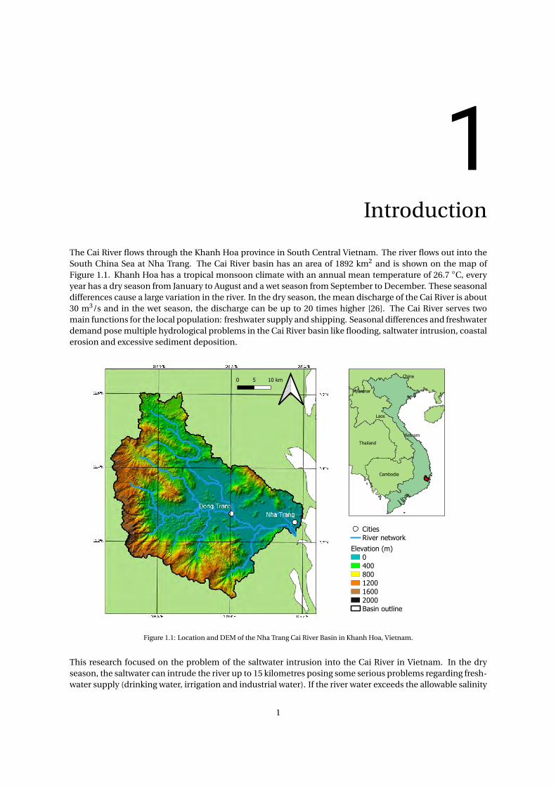
The Cai River flows through the Khanh Hoa province in South Central Vietnam. The river flows out into theSouth China Sea at Nha Trang. The Cai River basin has an area of 1892 km2 and is shown on the map ofFigure 1.1. Khanh Hoa has a tropical monsoon climate with an annual mean temperature of 26.7 ◦C, everyyear has a dry season from January to August and a wet season from September to December. These seasonaldifferences cause a large variation in the river. In the dry season, the mean discharge of the Cai River is about30 m3/s and in the wet season, the discharge can be up to 20 times higher [26]. The Cai River serves twomain functions for the local population: freshwater supply and shipping. Seasonal differences and freshwaterdemand pose multiple hydrological problems in the Cai River basin like flooding, saltwater intrusion, coastalerosion and excessive sediment deposition.
CitiesRiver network
Elevation (m)0400800120016002000Basin outline
Figure 1.1: Location and DEM of the Nha Trang Cai River Basin in Khanh Hoa, Vietnam.
This research focused on the problem of the saltwater intrusion into the Cai River in Vietnam. In the dryseason, the saltwater can intrude the river up to 15 kilometres posing some serious problems regarding fresh-water supply (drinking water, irrigation and industrial water). If the river water exceeds the allowable salinity
1
1.1. Research Goal and Questions 2
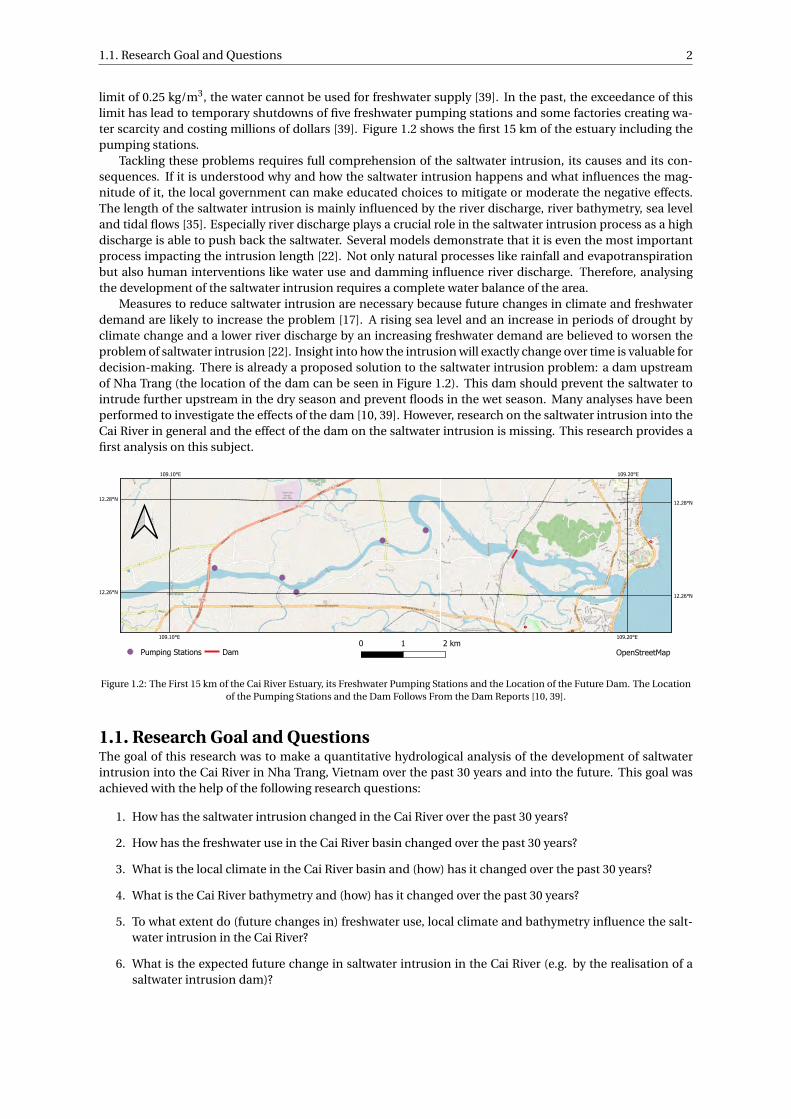
limit of 0.25 kg/m3, the water cannot be used for freshwater supply [39]. In the past, the exceedance of thislimit has lead to temporary shutdowns of five freshwater pumping stations and some factories creating wa-ter scarcity and costing millions of dollars [39]. Figure 1.2 shows the first 15 km of the estuary including thepumping stations.
Tackling these problems requires full comprehension of the saltwater intrusion, its causes and its con-sequences. If it is understood why and how the saltwater intrusion happens and what influences the mag-nitude of it, the local government can make educated choices to mitigate or moderate the negative effects.The length of the saltwater intrusion is mainly influenced by the river discharge, river bathymetry, sea leveland tidal flows [35]. Especially river discharge plays a crucial role in the saltwater intrusion process as a highdischarge is able to push back the saltwater. Several models demonstrate that it is even the most importantprocess impacting the intrusion length [22]. Not only natural processes like rainfall and evapotranspirationbut also human interventions like water use and damming influence river discharge. Therefore, analysingthe development of the saltwater intrusion requires a complete water balance of the area.
Measures to reduce saltwater intrusion are necessary because future changes in climate and freshwaterdemand are likely to increase the problem [17]. A rising sea level and an increase in periods of drought byclimate change and a lower river discharge by an increasing freshwater demand are believed to worsen theproblem of saltwater intrusion [22]. Insight into how the intrusion will exactly change over time is valuable fordecision-making. There is already a proposed solution to the saltwater intrusion problem: a dam upstreamof Nha Trang (the location of the dam can be seen in Figure 1.2). This dam should prevent the saltwater tointrude further upstream in the dry season and prevent floods in the wet season. Many analyses have beenperformed to investigate the effects of the dam [10, 39]. However, research on the saltwater intrusion into theCai River in general and the effect of the dam on the saltwater intrusion is missing. This research provides afirst analysis on this subject.
12.28°N12.28°N
12.26°N12.26°N
109.10°E
109.10°E
109.20°E
109.20°E
Pumping Stations Dam OpenStreetMap
Figure 1.2: The First 15 km of the Cai River Estuary, its Freshwater Pumping Stations and the Location of the Future Dam. The Locationof the Pumping Stations and the Dam Follows From the Dam Reports [10, 39].
1.1. Research Goal and QuestionsThe goal of this research was to make a quantitative hydrological analysis of the development of saltwaterintrusion into the Cai River in Nha Trang, Vietnam over the past 30 years and into the future. This goal wasachieved with the help of the following research questions:
1. How has the saltwater intrusion changed in the Cai River over the past 30 years?
2. How has the freshwater use in the Cai River basin changed over the past 30 years?
3. What is the local climate in the Cai River basin and (how) has it changed over the past 30 years?
4. What is the Cai River bathymetry and (how) has it changed over the past 30 years?
5. To what extent do (future changes in) freshwater use, local climate and bathymetry influence the salt-water intrusion in the Cai River?
6. What is the expected future change in saltwater intrusion in the Cai River (e.g. by the realisation of asaltwater intrusion dam)?
1.2. Methodology 3
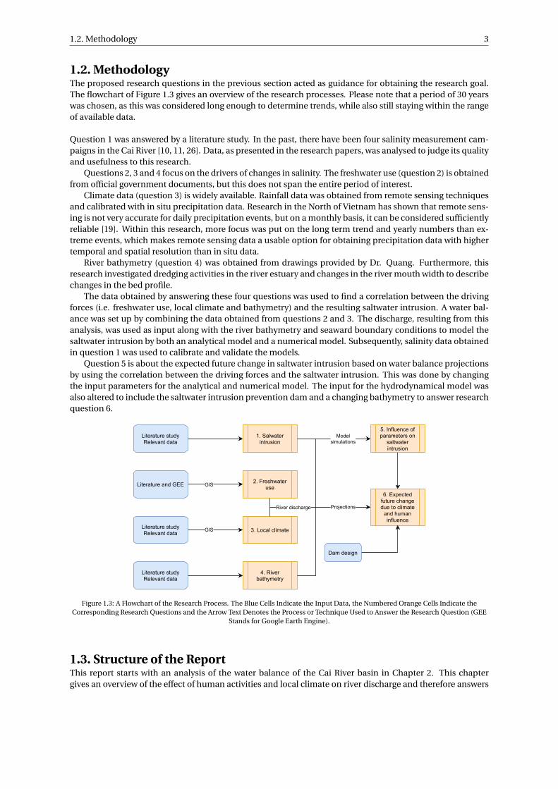
1.2. MethodologyThe proposed research questions in the previous section acted as guidance for obtaining the research goal.The flowchart of Figure 1.3 gives an overview of the research processes. Please note that a period of 30 yearswas chosen, as this was considered long enough to determine trends, while also still staying within the rangeof available data.
Question 1 was answered by a literature study. In the past, there have been four salinity measurement cam-paigns in the Cai River [10, 11, 26]. Data, as presented in the research papers, was analysed to judge its qualityand usefulness to this research.
Questions 2, 3 and 4 focus on the drivers of changes in salinity. The freshwater use (question 2) is obtainedfrom official government documents, but this does not span the entire period of interest.
Climate data (question 3) is widely available. Rainfall data was obtained from remote sensing techniquesand calibrated with in situ precipitation data. Research in the North of Vietnam has shown that remote sens-ing is not very accurate for daily precipitation events, but on a monthly basis, it can be considered sufficientlyreliable [19]. Within this research, more focus was put on the long term trend and yearly numbers than ex-treme events, which makes remote sensing data a usable option for obtaining precipitation data with highertemporal and spatial resolution than in situ data.
River bathymetry (question 4) was obtained from drawings provided by Dr. Quang. Furthermore, thisresearch investigated dredging activities in the river estuary and changes in the river mouth width to describechanges in the bed profile.
The data obtained by answering these four questions was used to find a correlation between the drivingforces (i.e. freshwater use, local climate and bathymetry) and the resulting saltwater intrusion. A water bal-ance was set up by combining the data obtained from questions 2 and 3. The discharge, resulting from thisanalysis, was used as input along with the river bathymetry and seaward boundary conditions to model thesaltwater intrusion by both an analytical model and a numerical model. Subsequently, salinity data obtainedin question 1 was used to calibrate and validate the models.
Question 5 is about the expected future change in saltwater intrusion based on water balance projectionsby using the correlation between the driving forces and the saltwater intrusion. This was done by changingthe input parameters for the analytical and numerical model. The input for the hydrodynamical model wasalso altered to include the saltwater intrusion prevention dam and a changing bathymetry to answer researchquestion 6.
1. Salwaterintrusion
2. Freshwateruse
3. Local climate
4. Riverbathymetry
Literature studyRelevant data
Literature and GEE
Literature studyRelevant data
Literature studyRelevant data
GIS
GIS
Modelsimulations
5. Influence ofparameters on
saltwaterintrusion
6. Expectedfuture changedue to climate
and humaninfluence
Projections
Dam design
River discharge
Figure 1.3: A Flowchart of the Research Process. The Blue Cells Indicate the Input Data, the Numbered Orange Cells Indicate theCorresponding Research Questions and the Arrow Text Denotes the Process or Technique Used to Answer the Research Question (GEE
Stands for Google Earth Engine).
1.3. Structure of the ReportThis report starts with an analysis of the water balance of the Cai River basin in Chapter 2. This chaptergives an overview of the effect of human activities and local climate on river discharge and therefore answers

1.3. Structure of the Report 4
research questions 2 and 3 by determining trends in freshwater use and local climate. In Chapter 3 the bound-ary conditions that are required for the models are given. This chapter answers also question 4 about the CaiRiver bathymetry. In both chapters 2 and 3, also projections for changes in the parameters are given at theend of the chapters. Next, Chapter 4 gives some relevant background information on saltwater intrusion aswell as collected salinity data of the Cai River. To answer question 1, an attempt was made to determine atrend in the extend of saltwater intrusion. All the above chapters form the basis to make an analytical andnumerical model of the saltwater intrusion. These models are introduced in Chapter 5 and their results arepresented and discussed in Chapter 6. The sensitivity of multiple parameters on the model was investigatedto make projections of the saltwater intrusion. This was done to answer research questions 5 and 6. Lastly,Chapter 7 provides conclusions and recommendations of this research.
2Water Balance
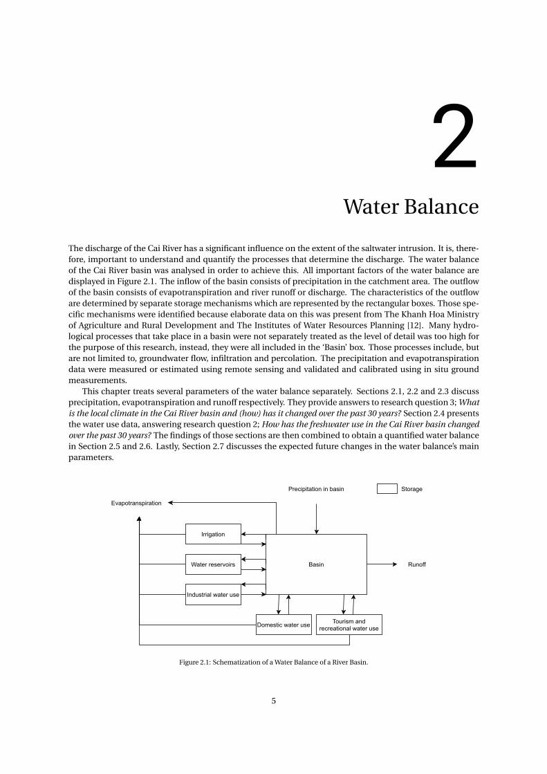
The discharge of the Cai River has a significant influence on the extent of the saltwater intrusion. It is, there-fore, important to understand and quantify the processes that determine the discharge. The water balanceof the Cai River basin was analysed in order to achieve this. All important factors of the water balance aredisplayed in Figure 2.1. The inflow of the basin consists of precipitation in the catchment area. The outflowof the basin consists of evapotranspiration and river runoff or discharge. The characteristics of the outfloware determined by separate storage mechanisms which are represented by the rectangular boxes. Those spe-cific mechanisms were identified because elaborate data on this was present from The Khanh Hoa Ministryof Agriculture and Rural Development and The Institutes of Water Resources Planning [12]. Many hydro-logical processes that take place in a basin were not separately treated as the level of detail was too high forthe purpose of this research, instead, they were all included in the ‘Basin’ box. Those processes include, butare not limited to, groundwater flow, infiltration and percolation. The precipitation and evapotranspirationdata were measured or estimated using remote sensing and validated and calibrated using in situ groundmeasurements.
This chapter treats several parameters of the water balance separately. Sections 2.1, 2.2 and 2.3 discussprecipitation, evapotranspiration and runoff respectively. They provide answers to research question 3; Whatis the local climate in the Cai River basin and (how) has it changed over the past 30 years? Section 2.4 presentsthe water use data, answering research question 2; How has the freshwater use in the Cai River basin changedover the past 30 years? The findings of those sections are then combined to obtain a quantified water balancein Section 2.5 and 2.6. Lastly, Section 2.7 discusses the expected future changes in the water balance’s mainparameters.
Basin
Irrigation
Evapotranspiration
Precipitation in basin
Runoff
Domestic water use
Industrial water use
Water reservoirs
Storage
Tourism andrecreational water use
Figure 2.1: Schematization of a Water Balance of a River Basin.
5
2.1. Rainfall 6
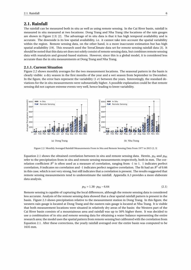
2.1. RainfallThe rainfall can be measured both in situ as well as using remote sensing. In the Cai River basin, rainfall ismeasured in situ measured at two locations: Dong Trang and Nha Trang (the locations of the rain gaugesare shown in Figure 2.3) [2]. The advantage of in situ data is that it has high temporal availability and isaccurate. The downside is its low spatial availability, i.e. it cannot take into account the spatial variabilitywithin the region. Remote sensing data, on the other hand, is a more inaccurate estimation but has highspatial availability [19]. This research used the TerraClimate data set for remote sensing rainfall data [3]. Itshould be noted that this data set does not solely consist of remote sensing data, but combines remote sensingdata with reanalysis and ground-based stations. However, since this is a global model, it is considered lessaccurate than the in situ measurements at Dong Trang and Nha Trang.
2.1.1. Current SituationFigure 2.2 shows monthly averages for the two measurement locations. The seasonal pattern in the basin isclearly visible: a dry season in the first months of the year and a wet season from September to December.In the figure, the error bars represent the variability (1 σ) between the years. Interestingly, the standard de-viations for the in situ measurements were substantially higher. A possible explanation could be that remotesensing did not capture extreme events very well, hence leading to lower variability.
Jan Feb Mar Apr May Jun Jul Aug Sep Oct Nov Dec0
100
200
300
400
500
600
Aver
age
Prec
ipita
tion
[mm
/mon
th]
In SituRemote Sensing
(a) Dong Trang
Jan Feb Mar Apr May Jun Jul Aug Sep Oct Nov Dec0
100
200
300
400
500
600Av
erag
e Pr
ecip
itatio
n [m
m/m
onth
]In SituRemote Sensing
(b) Nha Trang
Figure 2.2: Monthly Averaged Rainfall Measurements From in Situ and Remote Sensing Data From 1977 to 2015 [2, 3]
Equation 2.1 shows the obtained correlation between in situ and remote sensing data. Herein, pIS and pRS
refer to the precipitation from in situ and remote sensing measurements respectively, both in mm. The cor-relation coefficient R2 is often used as a measure of correlation, ranging from -1 to 1. 1 indicates perfectcorrelation, 0 indicates no correlation and -1 indicates perfect negative correlation. The fit had an R2 of 0.66in this case, which is not very strong, but still indicates that a correlation is present. The results suggested thatremote sensing measurements tend to underestimate the rainfall. Appendix A.3 provides a more elaboratedata analysis.
pIS = 1.38 ·pRS −6.64 (2.1)
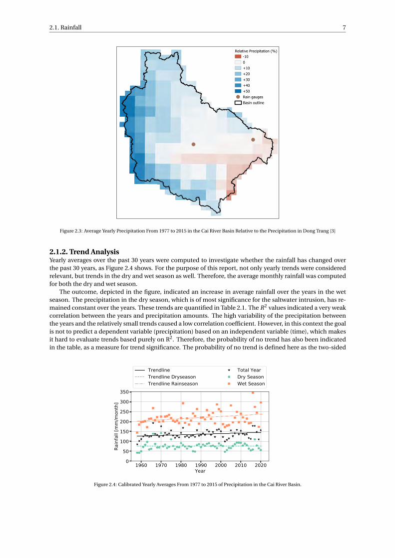
Remote sensing is capable of capturing the local differences, although the remote sensing data is consideredless accurate. Analysis of the remote sensing data showed that a clear spatial rainfall pattern is present in thebasin. Figure 2.3 shows precipitation relative to the measurement station in Dong Trang. In this figure, thewestern rain gauge is located at Dong Trang and the eastern rain gauge is located at Nha Trang. It is visiblethat both measurement locations were situated in relatively dry areas of the basin: the Western part of theCai River basin consists of a mountainous area and rainfall was up to 50% higher there. It was decided touse a combination of in situ and remote sensing data for obtaining a water balance representing the entireresearch area; the model uses the spatial pattern from remote sensing but calibrated with the correlation fromEquation 2.1. After these corrections, the yearly rainfall averaged over the entire basin was computed to be1635 mm.
2.1. Rainfall 7
Relative Precipitation (%)-10
0
+10
+20
+30
+40
+50
Rain gauges
Basin outline
Figure 2.3: Average Yearly Precipitation From 1977 to 2015 in the Cai River Basin Relative to the Precipitation in Dong Trang [3]
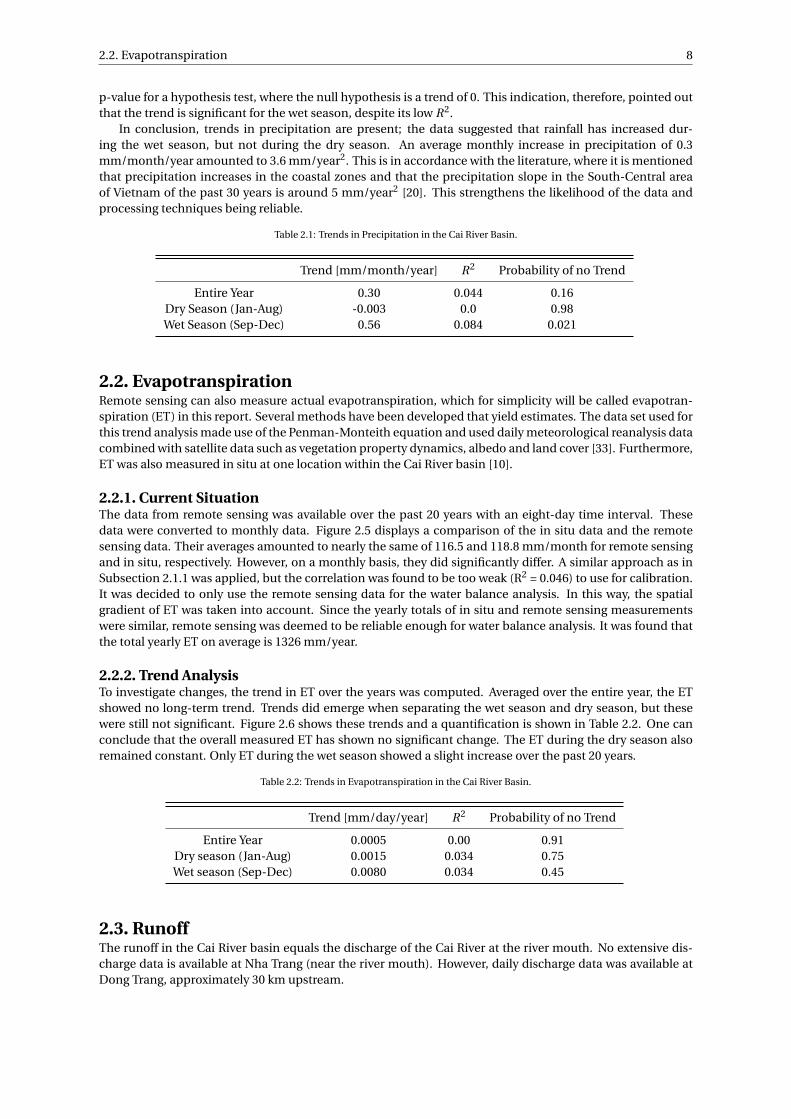
2.1.2. Trend AnalysisYearly averages over the past 30 years were computed to investigate whether the rainfall has changed overthe past 30 years, as Figure 2.4 shows. For the purpose of this report, not only yearly trends were consideredrelevant, but trends in the dry and wet season as well. Therefore, the average monthly rainfall was computedfor both the dry and wet season.
The outcome, depicted in the figure, indicated an increase in average rainfall over the years in the wetseason. The precipitation in the dry season, which is of most significance for the saltwater intrusion, has re-mained constant over the years. These trends are quantified in Table 2.1. The R2 values indicated a very weakcorrelation between the years and precipitation amounts. The high variability of the precipitation betweenthe years and the relatively small trends caused a low correlation coefficient. However, in this context the goalis not to predict a dependent variable (precipitation) based on an independent variable (time), which makesit hard to evaluate trends based purely on R2. Therefore, the probability of no trend has also been indicatedin the table, as a measure for trend significance. The probability of no trend is defined here as the two-sided
1960 1970 1980 1990 2000 2010 2020Year
0
50
100
150
200
250
300
350
Rain
fall
[mm
/mon
th]
TrendlineTrendline DryseasonTrendline Rainseason
Total YearDry SeasonWet Season
Figure 2.4: Calibrated Yearly Averages From 1977 to 2015 of Precipitation in the Cai River Basin.
2.2. Evapotranspiration 8
p-value for a hypothesis test, where the null hypothesis is a trend of 0. This indication, therefore, pointed outthat the trend is significant for the wet season, despite its low R2.
In conclusion, trends in precipitation are present; the data suggested that rainfall has increased dur-ing the wet season, but not during the dry season. An average monthly increase in precipitation of 0.3mm/month/year amounted to 3.6 mm/year2. This is in accordance with the literature, where it is mentionedthat precipitation increases in the coastal zones and that the precipitation slope in the South-Central areaof Vietnam of the past 30 years is around 5 mm/year2 [20]. This strengthens the likelihood of the data andprocessing techniques being reliable.
Table 2.1: Trends in Precipitation in the Cai River Basin.
Trend [mm/month/year] R2 Probability of no Trend
Entire Year 0.30 0.044 0.16Dry Season (Jan-Aug) -0.003 0.0 0.98Wet Season (Sep-Dec) 0.56 0.084 0.021
2.2. EvapotranspirationRemote sensing can also measure actual evapotranspiration, which for simplicity will be called evapotran-spiration (ET) in this report. Several methods have been developed that yield estimates. The data set used forthis trend analysis made use of the Penman-Monteith equation and used daily meteorological reanalysis datacombined with satellite data such as vegetation property dynamics, albedo and land cover [33]. Furthermore,ET was also measured in situ at one location within the Cai River basin [10].
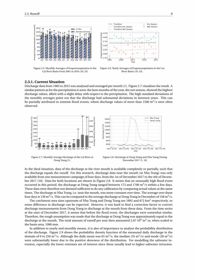
2.2.1. Current SituationThe data from remote sensing was available over the past 20 years with an eight-day time interval. Thesedata were converted to monthly data. Figure 2.5 displays a comparison of the in situ data and the remotesensing data. Their averages amounted to nearly the same of 116.5 and 118.8 mm/month for remote sensingand in situ, respectively. However, on a monthly basis, they did significantly differ. A similar approach as inSubsection 2.1.1 was applied, but the correlation was found to be too weak (R2 = 0.046) to use for calibration.It was decided to only use the remote sensing data for the water balance analysis. In this way, the spatialgradient of ET was taken into account. Since the yearly totals of in situ and remote sensing measurementswere similar, remote sensing was deemed to be reliable enough for water balance analysis. It was found thatthe total yearly ET on average is 1326 mm/year.
2.2.2. Trend AnalysisTo investigate changes, the trend in ET over the years was computed. Averaged over the entire year, the ETshowed no long-term trend. Trends did emerge when separating the wet season and dry season, but thesewere still not significant. Figure 2.6 shows these trends and a quantification is shown in Table 2.2. One canconclude that the overall measured ET has shown no significant change. The ET during the dry season alsoremained constant. Only ET during the wet season showed a slight increase over the past 20 years.
Table 2.2: Trends in Evapotranspiration in the Cai River Basin.
Trend [mm/day/year] R2 Probability of no Trend
Entire Year 0.0005 0.00 0.91Dry season (Jan-Aug) 0.0015 0.034 0.75Wet season (Sep-Dec) 0.0080 0.034 0.45
2.3. RunoffThe runoff in the Cai River basin equals the discharge of the Cai River at the river mouth. No extensive dis-charge data is available at Nha Trang (near the river mouth). However, daily discharge data was available atDong Trang, approximately 30 km upstream.
2.3. Runoff 9
Jan Feb Mar Apr May Jun Jul Aug Sep Oct Nov Dec0
20
40
60
80
100
120
140
160
Aver
age
Evap
otra
nspi
ratio
n [m
m/m
onth
]
In SituRemote Sensing
Figure 2.5: Monthly Averages of Evapotranspiration in theCai River Basin From 2001 to 2016 [10, 33]
2001 2006 2011 2016 2021Year
2.75
3.00
3.25
3.50
3.75
4.00
4.25
Evap
otra
nspi
ratio
n [m
m/d
ay]
TrendlineTrendline Dry SeasonTrendline Wet Season
Dry SeasonWet Season
Figure 2.6: Yearly Averages of Evapotranspiration in the CaiRiver Basin [10, 33].
2.3.1. Current SituationDischarge data from 1983 to 2012 was analysed and averaged per month [1]. Figure 2.7 visualises the result. Asimilar pattern as for the precipitation is seen; the lasts months of the year, the wet season, showed the highestdischarge values, albeit with a slight delay with respect to the precipitation. The high standard deviations ofthe monthly averages point out that the discharge had substantial deviations in between years. This canbe partially attributed to extreme flood events, where discharge values of more than 1500 m3/s were oftenobserved.
0
100
200
300
400
500
Aver
age
Mon
thly
Disc
harg
e [m
m]
Jan Feb Mar Apr May Jun Jul Aug Sep Oct Nov Dec050
100150200250300350400
Aver
age
Mon
thly
Disc
harg
e [m
3 /s]
Figure 2.7: Monthly Average Discharge of the Cai River atDong Trang [1].
2017-12-01 2017-12-02 2017-12-03 2017-12-04 2017-12-05Day
200400600800
1000120014001600
Disc
harg
e [m
3 /s]
Nha TrangDong Trang
Figure 2.8: Discharge at Dong Trang and Nha Trang DuringDecember 2017 [1, 10]
In the ideal situation, data of the discharge at the river mouth is available completely or partially, such thatthe discharge equals the runoff. For this research, discharge data near the mouth (at Nha Trang) was onlyavailable from one measurement campaign of four days, from the 1st of December 2017 to the 4th of Decem-ber 2017 [10]. Data for both locations are shown in Figure 2.8. It seems that an unusually high flood eventoccurred in this period; the discharge at Dong Trang ranged between 173 and 1700 m3/s within a few days.These data were therefore not deemed sufficient to do any calibration by comparing actual values at the sametimes. The discharge at Nha Trang, i.e. near the mouth, was more constant over time. The average over thesefour days is 139 m3/s. This can be compared to the average discharge at Dong Trang in December of 158 m3/s.
The catchment area sizes upstream of Nha Trang and Dong Trang are 1892 and 872 km2 respectively, sosome difference in discharge can be expected. However, it was hard to find a correction factor to convertdischarge measurements from Dong Trang to discharge at the mouth from these data. From the time seriesat the start of December 2017, it seems that before the flood event, the discharges were somewhat similar.Therefore, the rough assumption was made that the discharge at Dong Trang was approximately equal to thedischarge at the mouth. The total amount of runoff per year then amounted 2.07·109 m3 or, when scaled tothe basin area, 1080 mm.
In addition to yearly and monthly means, it is also of importance to analyse the probability distributionof the discharge. Figure 2.9 shows the probability density function of the measured daily discharge in thedomain of 0 to 250 m3/s. Although the daily mean was 65 m3/s, the median (35 m3/s) and mode (28 m3/s)were substantially lower due to the positive skewness of the distribution. For modelling the saltwater in-trusion, especially the lower extremes are of interest since these usually lead to higher saltwater intrusion.
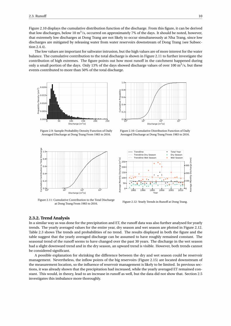
2.3. Runoff 10
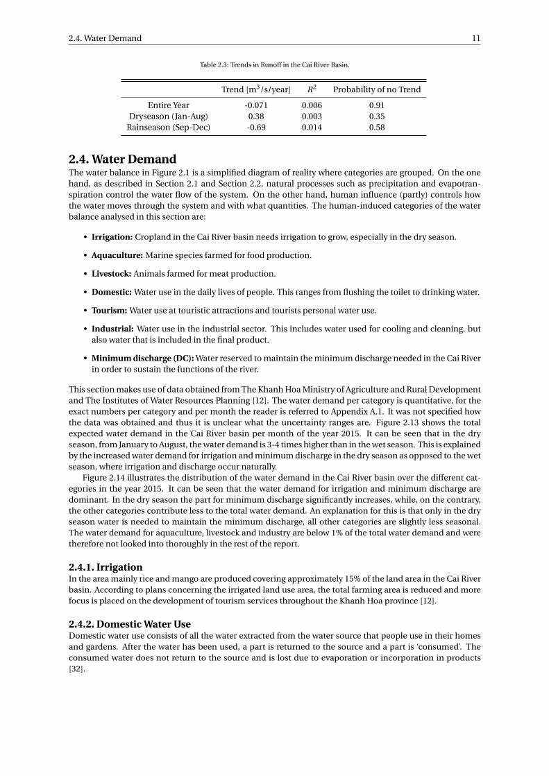
Figure 2.10 displays the cumulative distribution function of the discharge. From this figure, it can be derivedthat low discharges, below 10 m3/s, occurred on approximately 7% of the days. It should be noted, however,that extremely low discharges at Dong Trang are not likely to occur simultaneously at Nha Trang, since lowdischarges are mitigated by releasing water from water reservoirs downstream of Dong Trang (see Subsec-tion 2.4.4).
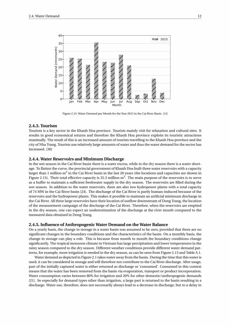
The low values are important for saltwater intrusion, but the high values are of more interest for the waterbalance. The cumulative contribution to the total discharge is shown in Figure 2.11 to further investigate thecontribution of high extremes. The figure points out how most runoff in the catchment happened duringonly a small portion of the days. Only 13% of the days showed discharge values of over 100 m3/s, but theseevents contributed to more than 50% of the total discharge.
0 50 100 150 200 250Discharge [m3/s]
0.000
0.005
0.010
0.015
0.020
Prop
abilit
y De
nsity
[s/m
3 ]
Figure 2.9: Sample Probability Density Function of DailyAveraged Discharge at Dong Trang From 1983 to 2016.
100 101 102 103
Discharge [m3/s]
0.0
0.2
0.4
0.6
0.8
1.0
Cum
ulat
ive
Prop
abilit
y
Figure 2.10: Cumulative Distribution Function of DailyAveraged Discharge at Dong Trang From 1983 to 2016.
100 101 102 103
Discharge [m3/s]
0.0
0.2
0.4
0.6
0.8
1.0
Cum
ulat
ive
Cont
ribut
ion
to T
otal
Disc
harg
e
Figure 2.11: Cumulative Contribution to the Total Dischargeat Dong Trang From 1983 to 2016.
0
100
200
300
Aver
age
Mon
thly
Disc
harg
e [m
m]
1985 1990 1995 2000 2005 2010Year
0
50
100
150
200
250
Aver
age
Mon
thly
Disc
harg
e [m
3 /s]
TrendlineTrendline Dry SeasonTrendline Wet Season
Total YearDry SeasonWet Season
Figure 2.12: Yearly Trends in Runoff at Dong Trang.
2.3.2. Trend AnalysisIn a similar way as was done for the precipitation and ET, the runoff data was also further analysed for yearlytrends. The yearly averaged values for the entire year, dry season and wet season are plotted in Figure 2.12.Table 2.3 shows The trends and probabilities of no trend. The results displayed in both the figure and thetable suggest that the yearly averaged discharge can be assumed to have roughly remained constant. Theseasonal trend of the runoff seems to have changed over the past 30 years. The discharge in the wet seasonhad a slight downward trend and in the dry season, an upward trend is visible. However, both trends cannotbe considered significant.
A possible explanation for shrinking the difference between the dry and wet season could be reservoirmanagement. Nevertheless, the inflow points of the big reservoirs (Figure 2.15) are located downstream ofthe measurement location, so the influence of reservoir management is likely to be limited. In previous sec-tions, it was already shown that the precipitation had increased, while the yearly averaged ET remained con-stant. This would, in theory, lead to an increase in runoff as well, but the data did not show that. Section 2.5investigates this imbalance more thoroughly.
2.4. Water Demand 11
Table 2.3: Trends in Runoff in the Cai River Basin.
Trend [m3/s/year] R2 Probability of no Trend
Entire Year -0.071 0.006 0.91Dryseason (Jan-Aug) 0.38 0.003 0.35
Rainseason (Sep-Dec) -0.69 0.014 0.58
2.4. Water DemandThe water balance in Figure 2.1 is a simplified diagram of reality where categories are grouped. On the onehand, as described in Section 2.1 and Section 2.2, natural processes such as precipitation and evapotran-spiration control the water flow of the system. On the other hand, human influence (partly) controls howthe water moves through the system and with what quantities. The human-induced categories of the waterbalance analysed in this section are:
• Irrigation: Cropland in the Cai River basin needs irrigation to grow, especially in the dry season.
• Aquaculture: Marine species farmed for food production.
• Livestock: Animals farmed for meat production.
• Domestic: Water use in the daily lives of people. This ranges from flushing the toilet to drinking water.
• Tourism: Water use at touristic attractions and tourists personal water use.
• Industrial: Water use in the industrial sector. This includes water used for cooling and cleaning, butalso water that is included in the final product.
• Minimum discharge (DC): Water reserved to maintain the minimum discharge needed in the Cai Riverin order to sustain the functions of the river.
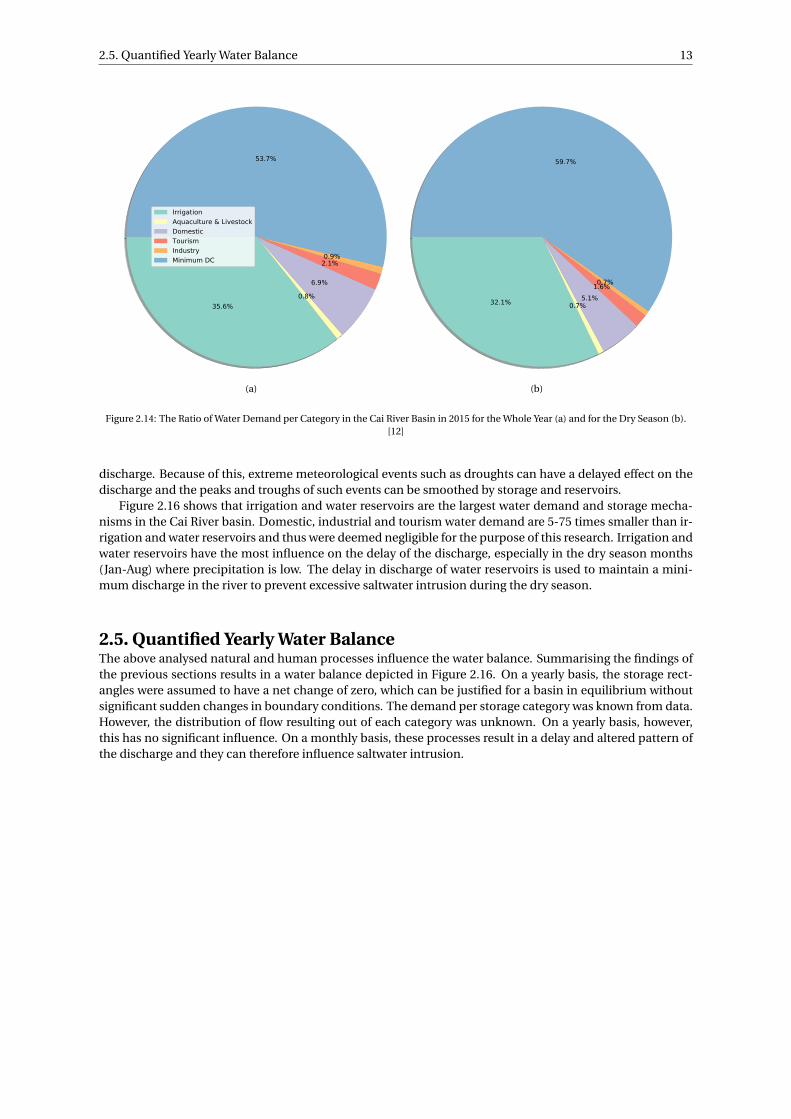
This section makes use of data obtained from The Khanh Hoa Ministry of Agriculture and Rural Developmentand The Institutes of Water Resources Planning [12]. The water demand per category is quantitative, for theexact numbers per category and per month the reader is referred to Appendix A.1. It was not specified howthe data was obtained and thus it is unclear what the uncertainty ranges are. Figure 2.13 shows the totalexpected water demand in the Cai River basin per month of the year 2015. It can be seen that in the dryseason, from January to August, the water demand is 3-4 times higher than in the wet season. This is explainedby the increased water demand for irrigation and minimum discharge in the dry season as opposed to the wetseason, where irrigation and discharge occur naturally.
Figure 2.14 illustrates the distribution of the water demand in the Cai River basin over the different cat-egories in the year 2015. It can be seen that the water demand for irrigation and minimum discharge aredominant. In the dry season the part for minimum discharge significantly increases, while, on the contrary,the other categories contribute less to the total water demand. An explanation for this is that only in the dryseason water is needed to maintain the minimum discharge, all other categories are slightly less seasonal.The water demand for aquaculture, livestock and industry are below 1% of the total water demand and weretherefore not looked into thoroughly in the rest of the report.
2.4.1. IrrigationIn the area mainly rice and mango are produced covering approximately 15% of the land area in the Cai Riverbasin. According to plans concerning the irrigated land use area, the total farming area is reduced and morefocus is placed on the development of tourism services throughout the Khanh Hoa province [12].
2.4.2. Domestic Water UseDomestic water use consists of all the water extracted from the water source that people use in their homesand gardens. After the water has been used, a part is returned to the source and a part is ‘consumed’. Theconsumed water does not return to the source and is lost due to evaporation or incorporation in products[32].
2.4. Water Demand 12
Jan Feb Mar Apr May Jun Jul Aug Sep Oct Nov DecMonth
0
5
10
15
20
25
30
35
40
Wat
er D
eman
d [m
m/m
onth
]
2015
Figure 2.13: Water Demand per Month for the Year 2015 in the Cai River Basin. [12]
2.4.3. TourismTourism is a key sector in the Khanh Hoa province. Tourists mainly visit for relaxation and cultural sites. Itresults in good economical returns and therefore the Khanh Hoa province exploits its touristic attractionsmaximally. The result of this is an increased amount of tourists travelling to the Khanh Hoa province and thecity of Nha Trang. Tourists use relatively large amounts of water and thus the water demand for the sector hasincreased. [30]
2.4.4. Water Reservoirs and Minimum DischargeIn the wet season in the Cai River basin there is a water excess, while in the dry season there is a water short-age. To flatten the curve, the provincial government of Khanh Hoa built three water reservoirs with a capacitylarger than 1 million m3 in the Cai River basin in the last 20 years (the locations and capacities are shown inFigure 2.15). Their total effective capacity is 35.3 million m3. The main purpose of the reservoirs is to serveas a buffer to maintain a sufficient freshwater supply in the dry season. The reservoirs are filled during thewet season. In addition to the water reservoirs, there are also two hydropower plants with a total capacityof 74 MW in the Cai River basin [24]. The discharge of the Cai River is partly human-induced because of thereservoirs and the hydropower plants. This makes it possible to maintain an artificial minimum discharge inthe Cai River. All three large reservoirs have their location of outflow downstream of Dong Trang, the locationof the measurement campaign of the discharge of the Cai River. Therefore, when the reservoirs are emptiedin the dry season, one can expect an underestimation of the discharge at the river mouth compared to themeasured data obtained in Dong Trang.
2.4.5. Influence of Anthropogenic Water Demand on the Water BalanceOn a yearly basis, the change in storage in a water basin was assumed to be zero, provided that there are nosignificant changes in the boundary conditions and the characteristics of the basin. On a monthly basis, thechange in storage can play a role. This is because from month to month the boundary conditions changesignificantly. The tropical monsoon climate in Vietnam has large precipitation and lower temperatures in therainy season compared to the dry season. Different weather conditions provide different water demand pat-terns, for example, more irrigation is needed in the dry season, as can be seen from Figure 2.13 and Table A.1.
Water demand as depicted in Figure 2.1 takes water away from the basin. During the time that this water isused, it can be considered in storage and will therefore not contribute to the Cai River discharge. After usage,part of the initially captured water is either returned as discharge or ‘consumed’. Consumed in this contextmeans that the water has been removed from the basin via evaporation, transport or product incorporation.Water consumption varies between 80% for irrigation and 20% for other domestic/anthropogenic demands[21]. So especially for demand types other than irrigation, a large part is returned to the basin resulting in adischarge. Water use, therefore, does not necessarily always lead to a decrease in discharge, but to a delay in
2.5. Quantified Yearly Water Balance 13
35.6%0.8%
6.9%
2.1%0.9%
53.7%
IrrigationAquaculture & LivestockDomesticTourismIndustryMinimum DC
(a)
32.1% 0.7%5.1%
1.6%0.7%
59.7%
(b)
Figure 2.14: The Ratio of Water Demand per Category in the Cai River Basin in 2015 for the Whole Year (a) and for the Dry Season (b).[12]
discharge. Because of this, extreme meteorological events such as droughts can have a delayed effect on thedischarge and the peaks and troughs of such events can be smoothed by storage and reservoirs.
Figure 2.16 shows that irrigation and water reservoirs are the largest water demand and storage mecha-nisms in the Cai River basin. Domestic, industrial and tourism water demand are 5-75 times smaller than ir-rigation and water reservoirs and thus were deemed negligible for the purpose of this research. Irrigation andwater reservoirs have the most influence on the delay of the discharge, especially in the dry season months(Jan-Aug) where precipitation is low. The delay in discharge of water reservoirs is used to maintain a mini-mum discharge in the river to prevent excessive saltwater intrusion during the dry season.
2.5. Quantified Yearly Water BalanceThe above analysed natural and human processes influence the water balance. Summarising the findings ofthe previous sections results in a water balance depicted in Figure 2.16. On a yearly basis, the storage rect-angles were assumed to have a net change of zero, which can be justified for a basin in equilibrium withoutsignificant sudden changes in boundary conditions. The demand per storage category was known from data.However, the distribution of flow resulting out of each category was unknown. On a yearly basis, however,this has no significant influence. On a monthly basis, these processes result in a delay and altered pattern ofthe discharge and they can therefore influence saltwater intrusion.
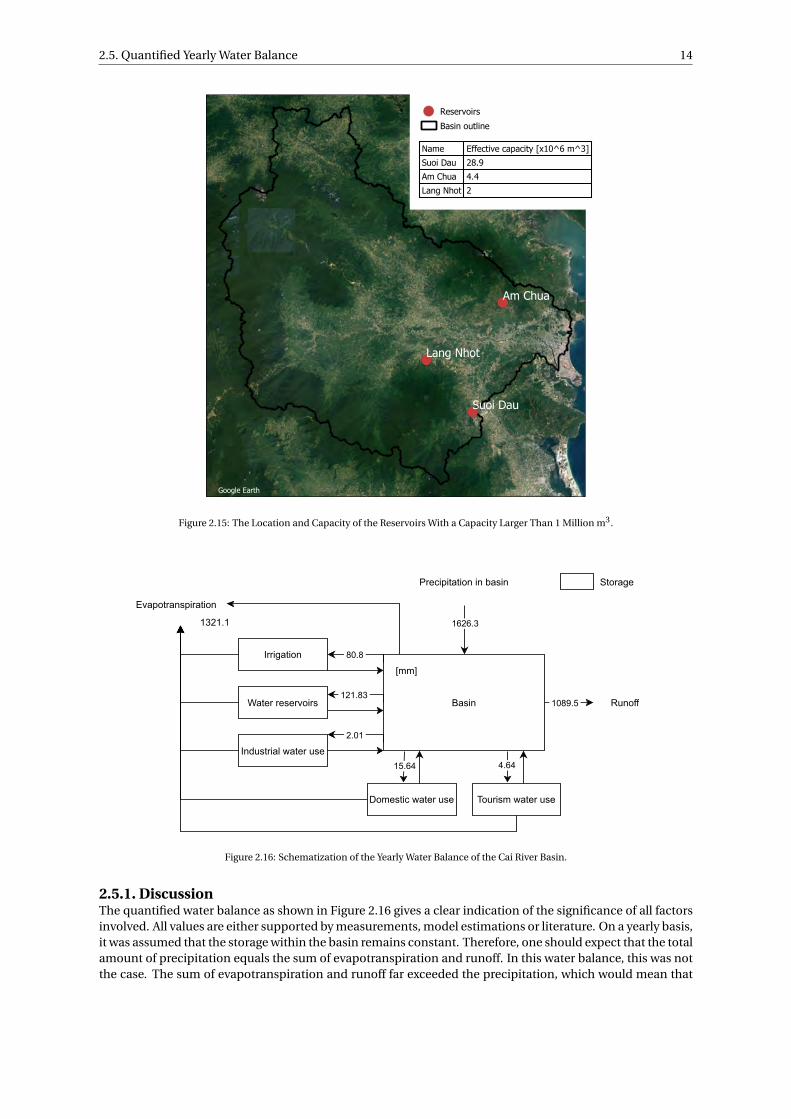
2.5. Quantified Yearly Water Balance 14
Reservoirs
Basin outline
Name Effective capacity [x10^6 m^3]
Suoi Dau 28.9
Am Chua 4.4
Lang Nhot 2
Google Earth
Figure 2.15: The Location and Capacity of the Reservoirs With a Capacity Larger Than 1 Million m3.
121.83 1089.5 Basin
Irrigation
Evapotranspiration
1626.3
Precipitation in basin
Runoff
Domestic water use
15.64Industrial water use
Water reservoirs
Storage
Tourism water use
4.64
2.01
80.8
1321.1
[mm]
Figure 2.16: Schematization of the Yearly Water Balance of the Cai River Basin.
2.5.1. DiscussionThe quantified water balance as shown in Figure 2.16 gives a clear indication of the significance of all factorsinvolved. All values are either supported by measurements, model estimations or literature. On a yearly basis,it was assumed that the storage within the basin remains constant. Therefore, one should expect that the totalamount of precipitation equals the sum of evapotranspiration and runoff. In this water balance, this was notthe case. The sum of evapotranspiration and runoff far exceeded the precipitation, which would mean that
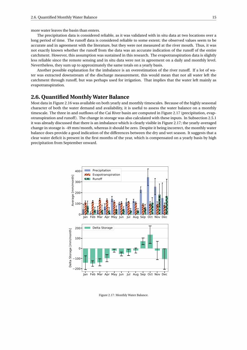
2.6. Quantified Monthly Water Balance 15
more water leaves the basin than enters.The precipitation data is considered reliable, as it was validated with in situ data at two locations over a
long period of time. The runoff data is considered reliable to some extent; the observed values seem to beaccurate and in agreement with the literature, but they were not measured at the river mouth. Thus, it wasnot exactly known whether the runoff from the data was an accurate indication of the runoff of the entirecatchment. However, this assumption was sustained in this research. The evapotranspiration data is slightlyless reliable since the remote sensing and in situ data were not in agreement on a daily and monthly level.Nevertheless, they sum up to approximately the same totals on a yearly basis.
Another possible explanation for the imbalance is an overestimation of the river runoff. If a lot of wa-ter was extracted downstream of the discharge measurement, this would mean that not all water left thecatchment through runoff, but was perhaps used for irrigation. That implies that the water left mainly asevapotranspiration.
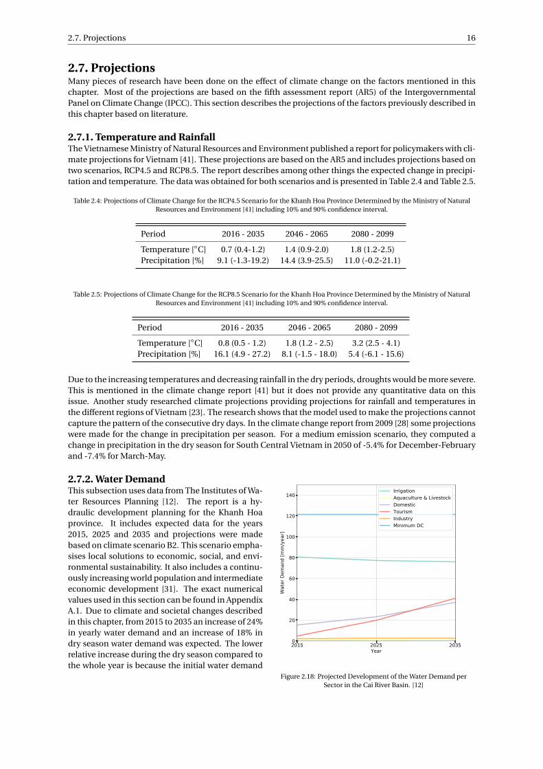
2.6. Quantified Monthly Water BalanceMost data in Figure 2.16 was available on both yearly and monthly timescales. Because of the highly seasonalcharacter of both the water demand and availability, it is useful to assess the water balance on a monthlytimescale. The three in and outflows of the Cai River basin are computed in Figure 2.17 (precipitation, evap-otranspiration and runoff). The change in storage was also calculated with these inputs. In Subsection 2.5.1it was already discussed that there is an imbalance which is clearly visible in Figure 2.17; the yearly-averagedchange in storage is -49 mm/month, whereas it should be zero. Despite it being incorrect, the monthly waterbalance does provide a good indication of the differences between the dry and wet season. It suggests that aclear water deficit is present in the first months of the year, which is compensated on a yearly basis by highprecipitation from September onward.
Jan Feb Mar Apr May Jun Jul Aug Sep Oct Nov Dec0
100
200
300
400
Aver
age
[mm
/mon
th]
PrecipitationEvapotranspirationRunoff
Jan Feb Mar Apr May Jun Jul Aug Sep Oct Nov Dec200
100
0
100
200
Delta
Sto
rage
[mm
/mon
th] Delta Storage
Figure 2.17: Monthly Water Balance.
2.7. Projections 16
2.7. ProjectionsMany pieces of research have been done on the effect of climate change on the factors mentioned in thischapter. Most of the projections are based on the fifth assessment report (AR5) of the IntergovernmentalPanel on Climate Change (IPCC). This section describes the projections of the factors previously described inthis chapter based on literature.
2.7.1. Temperature and RainfallThe Vietnamese Ministry of Natural Resources and Environment published a report for policymakers with cli-mate projections for Vietnam [41]. These projections are based on the AR5 and includes projections based ontwo scenarios, RCP4.5 and RCP8.5. The report describes among other things the expected change in precipi-tation and temperature. The data was obtained for both scenarios and is presented in Table 2.4 and Table 2.5.
Table 2.4: Projections of Climate Change for the RCP4.5 Scenario for the Khanh Hoa Province Determined by the Ministry of NaturalResources and Environment [41] including 10% and 90% confidence interval.
Period 2016 - 2035 2046 - 2065 2080 - 2099
Temperature [◦C] 0.7 (0.4-1.2) 1.4 (0.9-2.0) 1.8 (1.2-2.5)Precipitation [%] 9.1 (-1.3-19.2) 14.4 (3.9-25.5) 11.0 (-0.2-21.1)
Table 2.5: Projections of Climate Change for the RCP8.5 Scenario for the Khanh Hoa Province Determined by the Ministry of NaturalResources and Environment [41] including 10% and 90% confidence interval.
Period 2016 - 2035 2046 - 2065 2080 - 2099
Temperature [◦C] 0.8 (0.5 - 1.2) 1.8 (1.2 - 2.5) 3.2 (2.5 - 4.1)Precipitation [%] 16.1 (4.9 - 27.2) 8.1 (-1.5 - 18.0) 5.4 (-6.1 - 15.6)
Due to the increasing temperatures and decreasing rainfall in the dry periods, droughts would be more severe.This is mentioned in the climate change report [41] but it does not provide any quantitative data on thisissue. Another study researched climate projections providing projections for rainfall and temperatures inthe different regions of Vietnam [23]. The research shows that the model used to make the projections cannotcapture the pattern of the consecutive dry days. In the climate change report from 2009 [28] some projectionswere made for the change in precipitation per season. For a medium emission scenario, they computed achange in precipitation in the dry season for South Central Vietnam in 2050 of -5.4% for December-Februaryand -7.4% for March-May.
2.7.2. Water Demand
2015 2025 2035Year
0
20
40
60
80
100
120
140
Wat
er D
eman
d [m
m/y
ear]
IrrigationAquaculture & LivestockDomesticTourismIndustryMinimum DC
Figure 2.18: Projected Development of the Water Demand perSector in the Cai River Basin. [12]
This subsection uses data from The Institutes of Wa-ter Resources Planning [12]. The report is a hy-draulic development planning for the Khanh Hoaprovince. It includes expected data for the years2015, 2025 and 2035 and projections were madebased on climate scenario B2. This scenario empha-sises local solutions to economic, social, and envi-ronmental sustainability. It also includes a continu-ously increasing world population and intermediateeconomic development [31]. The exact numericalvalues used in this section can be found in AppendixA.1. Due to climate and societal changes describedin this chapter, from 2015 to 2035 an increase of 24%in yearly water demand and an increase of 18% indry season water demand was expected. The lowerrelative increase during the dry season compared tothe whole year is because the initial water demand
2.8. Conclusions on the Water Balance 17
in the dry season is higher. Even if the absolute in-crease was higher, the relative increase can be lower. Figure 2.18 shows the absolute expected increase persector until 2035. It can be seen that the growth in demand mainly comes from domestic and tourism waterdemand. Irrigation is projected to slightly decrease and minimum discharge is projected to stay the same.The other categories are insignificant compared with the other categories. This justifies the statement madein Section 2.4 to not treat these categories in more depth.
The demand for minimum discharge is larger in the wet season than in the dry season. More informationon this subject can be found in Appendix A.1. Furthermore, it was found that the four main categories con-tributing to the total demand are irrigation, minimum discharge, domestic and tourism. Of which over theyears the part for irrigation and discharge is expected to decrease and the part for tourism and domestic isexpected to increase as a portion of the total water demand in the Cai River basin.
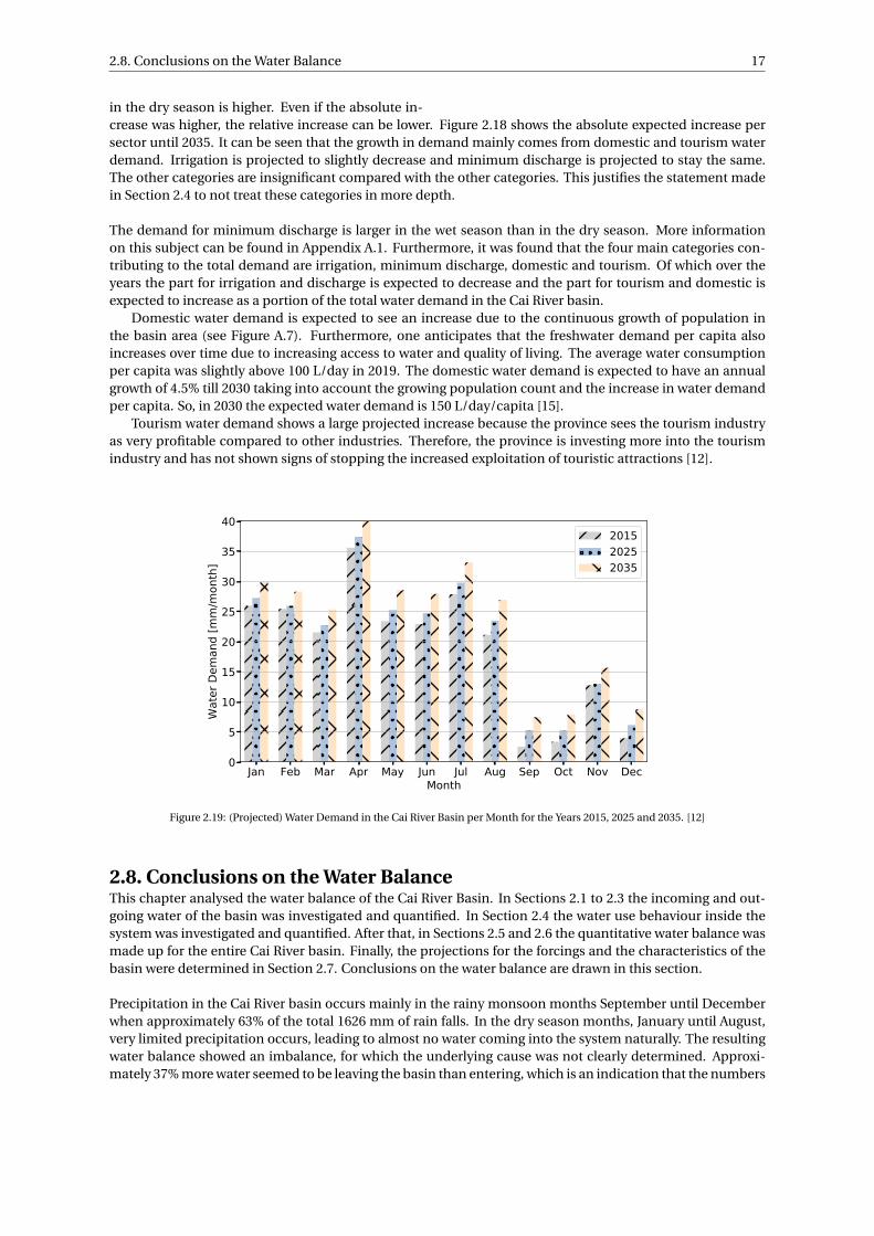
Domestic water demand is expected to see an increase due to the continuous growth of population inthe basin area (see Figure A.7). Furthermore, one anticipates that the freshwater demand per capita alsoincreases over time due to increasing access to water and quality of living. The average water consumptionper capita was slightly above 100 L/day in 2019. The domestic water demand is expected to have an annualgrowth of 4.5% till 2030 taking into account the growing population count and the increase in water demandper capita. So, in 2030 the expected water demand is 150 L/day/capita [15].
Tourism water demand shows a large projected increase because the province sees the tourism industryas very profitable compared to other industries. Therefore, the province is investing more into the tourismindustry and has not shown signs of stopping the increased exploitation of touristic attractions [12].
Jan Feb Mar Apr May Jun Jul Aug Sep Oct Nov DecMonth
0
5
10
15
20
25
30
35
40
Wat
er D
eman
d [m
m/m
onth
]
201520252035
Figure 2.19: (Projected) Water Demand in the Cai River Basin per Month for the Years 2015, 2025 and 2035. [12]
2.8. Conclusions on the Water BalanceThis chapter analysed the water balance of the Cai River Basin. In Sections 2.1 to 2.3 the incoming and out-going water of the basin was investigated and quantified. In Section 2.4 the water use behaviour inside thesystem was investigated and quantified. After that, in Sections 2.5 and 2.6 the quantitative water balance wasmade up for the entire Cai River basin. Finally, the projections for the forcings and the characteristics of thebasin were determined in Section 2.7. Conclusions on the water balance are drawn in this section.
Precipitation in the Cai River basin occurs mainly in the rainy monsoon months September until Decemberwhen approximately 63% of the total 1626 mm of rain falls. In the dry season months, January until August,very limited precipitation occurs, leading to almost no water coming into the system naturally. The resultingwater balance showed an imbalance, for which the underlying cause was not clearly determined. Approxi-mately 37% more water seemed to be leaving the basin than entering, which is an indication that the numbers
2.8. Conclusions on the Water Balance 18
used were not correct. The discharge data is the most likely source of error of all parameters. Nevertheless,the obtained numbers do provide valuable insights in the orders of magnitudes of all factors involved.
Water is used within the basin system in various ways by different sectors such as farming, industry andtourism. Furthermore, water is stored in water reservoirs until needed. On a yearly time scale, the influenceof the water demand per sector on the discharge of the Cai River is insignificant, as almost all water returnsto the river after use. However, the effect of the water demand on the discharge is notable on a monthly basis.A large part of the runoff in the dry season is human-controlled through the release of water from waterreservoirs. The part of the runoff due to water reservoirs is approximately 50% of the total average runoff permonth in the dry season. This is a rough estimation and it is not known when the water is released exactly. Itwas, therefore, not possible with the current data to take into account the outflow of these reservoirs.
Projections and trend analyses of the water demand, precipitation and evapotranspiration gave moreinsight into the development of the system into the future. It was concluded that precipitation is likely toincrease and evapotranspiration is likely to remain constant. The projected increase in precipitation is ex-pected to mainly occur in the wet season. Furthermore, the water demand was projected to increase duringall months of the year. Domestic and tourism water are the main increasing sectors, whilst the other sectorsapproximately remain the same. From the water balance, water demand and the projections it was concludedthat in the future there is going to be more discharge running through the Cai River on a yearly basis due tothe increased precipitation. The water stress could increase due to an increase in water demand and no sig-nificant increase in precipitation in the dry season.
It was not possible to directly model the discharge per month as a function of the system characteristics andthe boundary conditions accurately enough to model the saltwater intrusion because of the aforementionedknowledge gaps in the water balance of the Cai River basin. Qualitative analyses can be done as much aboutthe system was known and trends into the future have also been determined. In the remainder of the report,the influence of the system parameters on saltwater intrusion is determined using analytical and numericalmodels. The link is made between the influence of the discharge on the saltwater intrusion and the qualita-tive development of the discharge as was explained in this chapter.
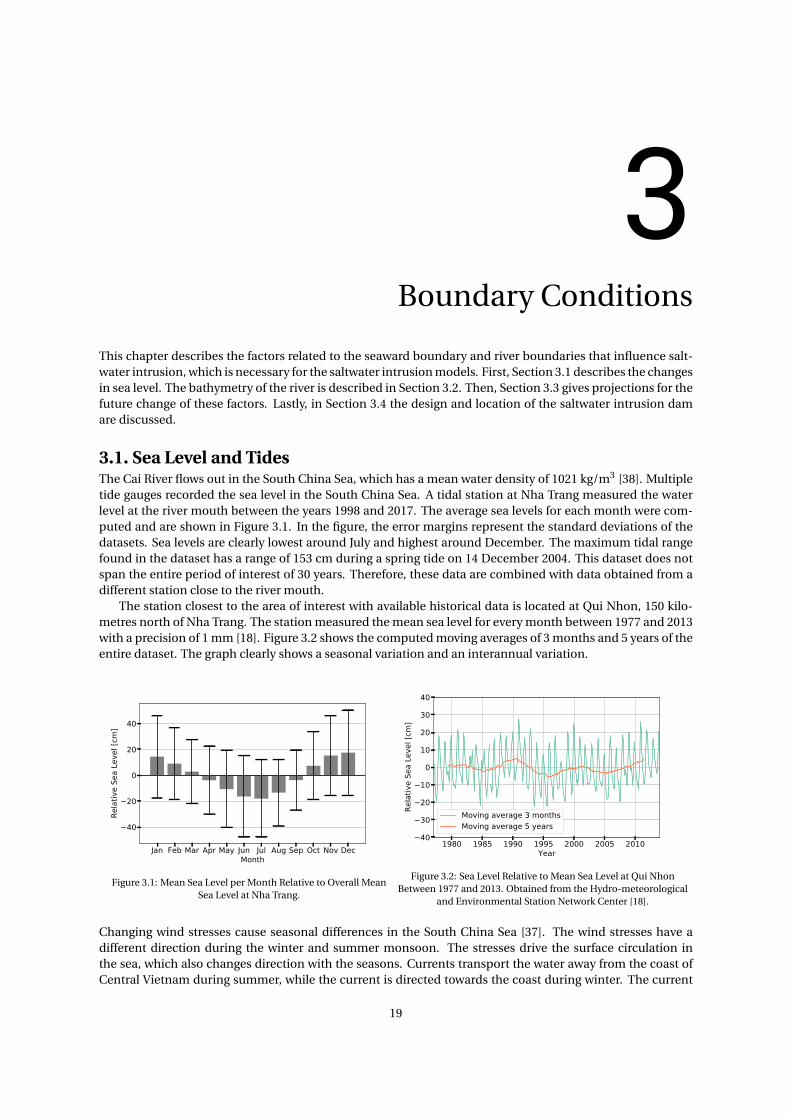
3Boundary Conditions
This chapter describes the factors related to the seaward boundary and river boundaries that influence salt-water intrusion, which is necessary for the saltwater intrusion models. First, Section 3.1 describes the changesin sea level. The bathymetry of the river is described in Section 3.2. Then, Section 3.3 gives projections for thefuture change of these factors. Lastly, in Section 3.4 the design and location of the saltwater intrusion damare discussed.
3.1. Sea Level and TidesThe Cai River flows out in the South China Sea, which has a mean water density of 1021 kg/m3 [38]. Multipletide gauges recorded the sea level in the South China Sea. A tidal station at Nha Trang measured the waterlevel at the river mouth between the years 1998 and 2017. The average sea levels for each month were com-puted and are shown in Figure 3.1. In the figure, the error margins represent the standard deviations of thedatasets. Sea levels are clearly lowest around July and highest around December. The maximum tidal rangefound in the dataset has a range of 153 cm during a spring tide on 14 December 2004. This dataset does notspan the entire period of interest of 30 years. Therefore, these data are combined with data obtained from adifferent station close to the river mouth.
The station closest to the area of interest with available historical data is located at Qui Nhon, 150 kilo-metres north of Nha Trang. The station measured the mean sea level for every month between 1977 and 2013with a precision of 1 mm [18]. Figure 3.2 shows the computed moving averages of 3 months and 5 years of theentire dataset. The graph clearly shows a seasonal variation and an interannual variation.
Jan Feb Mar Apr May Jun Jul Aug Sep Oct Nov DecMonth
40
20
0
20
40
Rela
tive
Sea
Leve
l [cm
]
Figure 3.1: Mean Sea Level per Month Relative to Overall MeanSea Level at Nha Trang.
1980 1985 1990 1995 2000 2005 2010Year
40
30
20
10
0
10
20
30
40
Rela
tive
Sea
Leve
l [cm
]
Moving average 3 monthsMoving average 5 years
Figure 3.2: Sea Level Relative to Mean Sea Level at Qui NhonBetween 1977 and 2013. Obtained from the Hydro-meteorological
and Environmental Station Network Center [18].
Changing wind stresses cause seasonal differences in the South China Sea [37]. The wind stresses have adifferent direction during the winter and summer monsoon. The stresses drive the surface circulation inthe sea, which also changes direction with the seasons. Currents transport the water away from the coast ofCentral Vietnam during summer, while the current is directed towards the coast during winter. The current
19
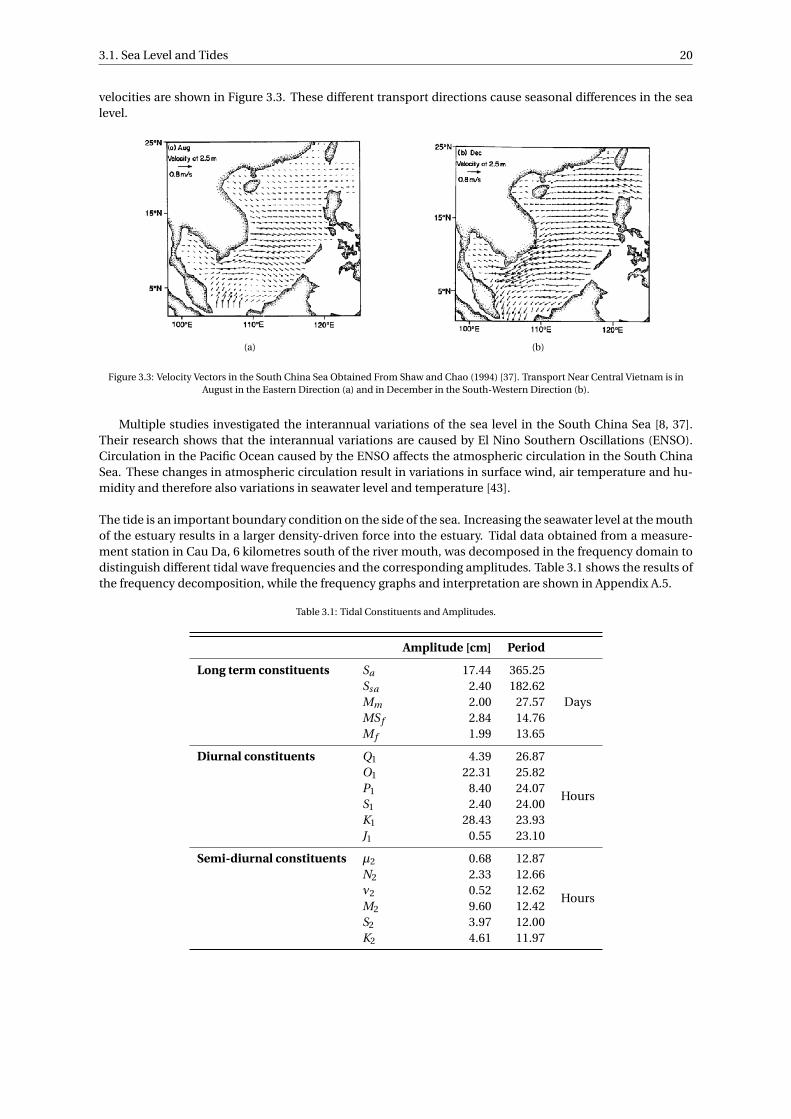
3.1. Sea Level and Tides 20
velocities are shown in Figure 3.3. These different transport directions cause seasonal differences in the sealevel.
(a) (b)
Figure 3.3: Velocity Vectors in the South China Sea Obtained From Shaw and Chao (1994) [37]. Transport Near Central Vietnam is inAugust in the Eastern Direction (a) and in December in the South-Western Direction (b).
Multiple studies investigated the interannual variations of the sea level in the South China Sea [8, 37].Their research shows that the interannual variations are caused by El Nino Southern Oscillations (ENSO).Circulation in the Pacific Ocean caused by the ENSO affects the atmospheric circulation in the South ChinaSea. These changes in atmospheric circulation result in variations in surface wind, air temperature and hu-midity and therefore also variations in seawater level and temperature [43].
The tide is an important boundary condition on the side of the sea. Increasing the seawater level at the mouthof the estuary results in a larger density-driven force into the estuary. Tidal data obtained from a measure-ment station in Cau Da, 6 kilometres south of the river mouth, was decomposed in the frequency domain todistinguish different tidal wave frequencies and the corresponding amplitudes. Table 3.1 shows the results ofthe frequency decomposition, while the frequency graphs and interpretation are shown in Appendix A.5.
Table 3.1: Tidal Constituents and Amplitudes.
Amplitude [cm] Period
Long term constituents Sa 17.44 365.25
DaysSsa 2.40 182.62Mm 2.00 27.57MS f 2.84 14.76M f 1.99 13.65
Diurnal constituents Q1 4.39 26.87
Hours
O1 22.31 25.82P1 8.40 24.07S1 2.40 24.00K1 28.43 23.93J1 0.55 23.10
Semi-diurnal constituents µ2 0.68 12.87
Hours
N2 2.33 12.66ν2 0.52 12.62M2 9.60 12.42S2 3.97 12.00K2 4.61 11.97
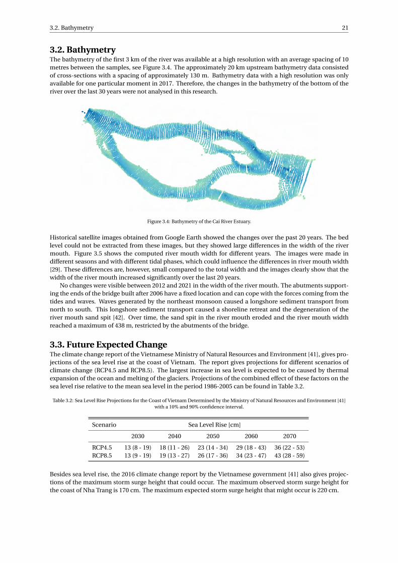
3.2. Bathymetry 21
3.2. BathymetryThe bathymetry of the first 3 km of the river was available at a high resolution with an average spacing of 10metres between the samples, see Figure 3.4. The approximately 20 km upstream bathymetry data consistedof cross-sections with a spacing of approximately 130 m. Bathymetry data with a high resolution was onlyavailable for one particular moment in 2017. Therefore, the changes in the bathymetry of the bottom of theriver over the last 30 years were not analysed in this research.
Figure 3.4: Bathymetry of the Cai River Estuary.
Historical satellite images obtained from Google Earth showed the changes over the past 20 years. The bedlevel could not be extracted from these images, but they showed large differences in the width of the rivermouth. Figure 3.5 shows the computed river mouth width for different years. The images were made indifferent seasons and with different tidal phases, which could influence the differences in river mouth width[29]. These differences are, however, small compared to the total width and the images clearly show that thewidth of the river mouth increased significantly over the last 20 years.
No changes were visible between 2012 and 2021 in the width of the river mouth. The abutments support-ing the ends of the bridge built after 2006 have a fixed location and can cope with the forces coming from thetides and waves. Waves generated by the northeast monsoon caused a longshore sediment transport fromnorth to south. This longshore sediment transport caused a shoreline retreat and the degeneration of theriver mouth sand spit [42]. Over time, the sand spit in the river mouth eroded and the river mouth widthreached a maximum of 438 m, restricted by the abutments of the bridge.
3.3. Future Expected ChangeThe climate change report of the Vietnamese Ministry of Natural Resources and Environment [41], gives pro-jections of the sea level rise at the coast of Vietnam. The report gives projections for different scenarios ofclimate change (RCP4.5 and RCP8.5). The largest increase in sea level is expected to be caused by thermalexpansion of the ocean and melting of the glaciers. Projections of the combined effect of these factors on thesea level rise relative to the mean sea level in the period 1986-2005 can be found in Table 3.2.
Table 3.2: Sea Level Rise Projections for the Coast of Vietnam Determined by the Ministry of Natural Resources and Environment [41]with a 10% and 90% confidence interval.
Scenario Sea Level Rise [cm]
2030 2040 2050 2060 2070
RCP4.5 13 (8 - 19) 18 (11 - 26) 23 (14 - 34) 29 (18 - 43) 36 (22 - 53)RCP8.5 13 (9 - 19) 19 (13 - 27) 26 (17 - 36) 34 (23 - 47) 43 (28 - 59)
Besides sea level rise, the 2016 climate change report by the Vietnamese government [41] also gives projec-tions of the maximum storm surge height that could occur. The maximum observed storm surge height forthe coast of Nha Trang is 170 cm. The maximum expected storm surge height that might occur is 220 cm.
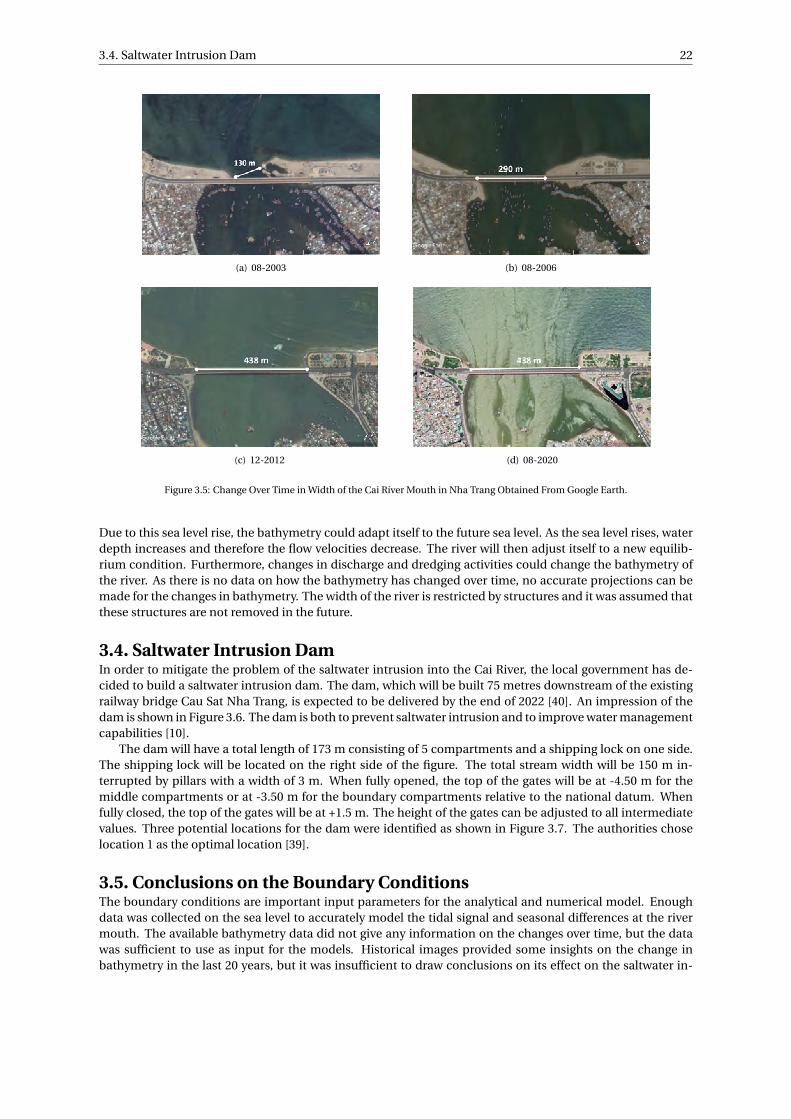
3.4. Saltwater Intrusion Dam 22
(a) 08-2003 (b) 08-2006
(c) 12-2012 (d) 08-2020
Figure 3.5: Change Over Time in Width of the Cai River Mouth in Nha Trang Obtained From Google Earth.
Due to this sea level rise, the bathymetry could adapt itself to the future sea level. As the sea level rises, waterdepth increases and therefore the flow velocities decrease. The river will then adjust itself to a new equilib-rium condition. Furthermore, changes in discharge and dredging activities could change the bathymetry ofthe river. As there is no data on how the bathymetry has changed over time, no accurate projections can bemade for the changes in bathymetry. The width of the river is restricted by structures and it was assumed thatthese structures are not removed in the future.
3.4. Saltwater Intrusion DamIn order to mitigate the problem of the saltwater intrusion into the Cai River, the local government has de-cided to build a saltwater intrusion dam. The dam, which will be built 75 metres downstream of the existingrailway bridge Cau Sat Nha Trang, is expected to be delivered by the end of 2022 [40]. An impression of thedam is shown in Figure 3.6. The dam is both to prevent saltwater intrusion and to improve water managementcapabilities [10].
The dam will have a total length of 173 m consisting of 5 compartments and a shipping lock on one side.The shipping lock will be located on the right side of the figure. The total stream width will be 150 m in-terrupted by pillars with a width of 3 m. When fully opened, the top of the gates will be at -4.50 m for themiddle compartments or at -3.50 m for the boundary compartments relative to the national datum. Whenfully closed, the top of the gates will be at +1.5 m. The height of the gates can be adjusted to all intermediatevalues. Three potential locations for the dam were identified as shown in Figure 3.7. The authorities choselocation 1 as the optimal location [39].
3.5. Conclusions on the Boundary ConditionsThe boundary conditions are important input parameters for the analytical and numerical model. Enoughdata was collected on the sea level to accurately model the tidal signal and seasonal differences at the rivermouth. The available bathymetry data did not give any information on the changes over time, but the datawas sufficient to use as input for the models. Historical images provided some insights on the change inbathymetry in the last 20 years, but it was insufficient to draw conclusions on its effect on the saltwater in-
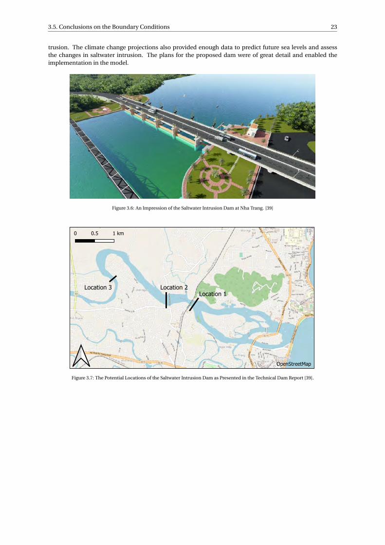
3.5. Conclusions on the Boundary Conditions 23
trusion. The climate change projections also provided enough data to predict future sea levels and assessthe changes in saltwater intrusion. The plans for the proposed dam were of great detail and enabled theimplementation in the model.
Figure 3.6: An Impression of the Saltwater Intrusion Dam at Nha Trang. [39]
OpenStreetMap
Location 1Location 2Location 3
Figure 3.7: The Potential Locations of the Saltwater Intrusion Dam as Presented in the Technical Dam Report [39].
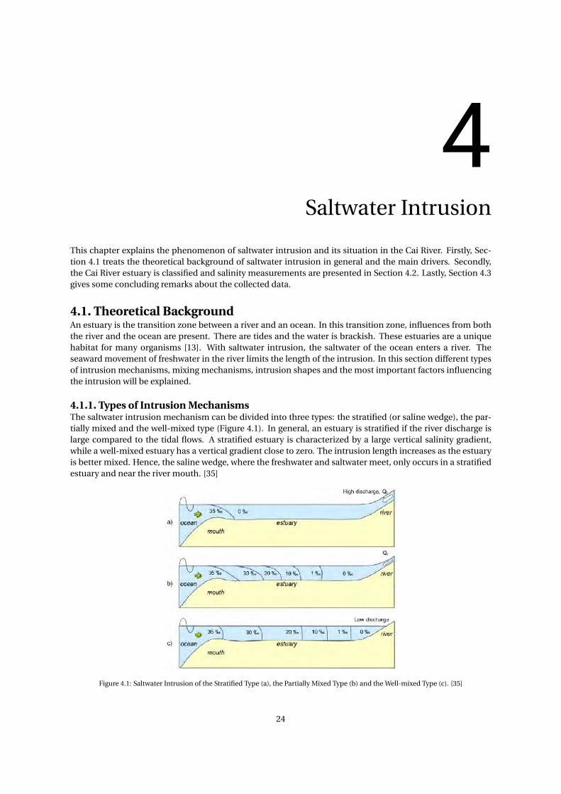
4Saltwater Intrusion
This chapter explains the phenomenon of saltwater intrusion and its situation in the Cai River. Firstly, Sec-tion 4.1 treats the theoretical background of saltwater intrusion in general and the main drivers. Secondly,the Cai River estuary is classified and salinity measurements are presented in Section 4.2. Lastly, Section 4.3gives some concluding remarks about the collected data.
4.1. Theoretical BackgroundAn estuary is the transition zone between a river and an ocean. In this transition zone, influences from boththe river and the ocean are present. There are tides and the water is brackish. These estuaries are a uniquehabitat for many organisms [13]. With saltwater intrusion, the saltwater of the ocean enters a river. Theseaward movement of freshwater in the river limits the length of the intrusion. In this section different typesof intrusion mechanisms, mixing mechanisms, intrusion shapes and the most important factors influencingthe intrusion will be explained.
4.1.1. Types of Intrusion MechanismsThe saltwater intrusion mechanism can be divided into three types: the stratified (or saline wedge), the par-tially mixed and the well-mixed type (Figure 4.1). In general, an estuary is stratified if the river discharge islarge compared to the tidal flows. A stratified estuary is characterized by a large vertical salinity gradient,while a well-mixed estuary has a vertical gradient close to zero. The intrusion length increases as the estuaryis better mixed. Hence, the saline wedge, where the freshwater and saltwater meet, only occurs in a stratifiedestuary and near the river mouth. [35]
Figure 4.1: Saltwater Intrusion of the Stratified Type (a), the Partially Mixed Type (b) and the Well-mixed Type (c). [35]
24
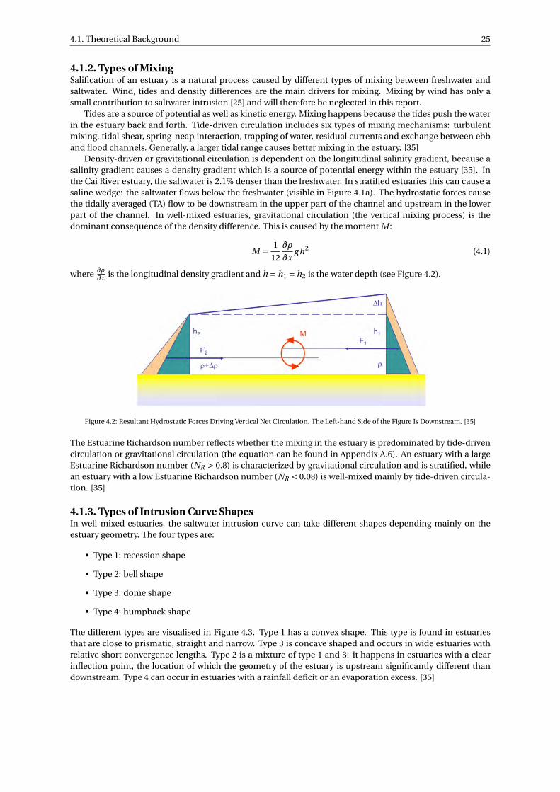
4.1. Theoretical Background 25
4.1.2. Types of MixingSalification of an estuary is a natural process caused by different types of mixing between freshwater andsaltwater. Wind, tides and density differences are the main drivers for mixing. Mixing by wind has only asmall contribution to saltwater intrusion [25] and will therefore be neglected in this report.
Tides are a source of potential as well as kinetic energy. Mixing happens because the tides push the waterin the estuary back and forth. Tide-driven circulation includes six types of mixing mechanisms: turbulentmixing, tidal shear, spring-neap interaction, trapping of water, residual currents and exchange between ebband flood channels. Generally, a larger tidal range causes better mixing in the estuary. [35]
Density-driven or gravitational circulation is dependent on the longitudinal salinity gradient, because asalinity gradient causes a density gradient which is a source of potential energy within the estuary [35]. Inthe Cai River estuary, the saltwater is 2.1% denser than the freshwater. In stratified estuaries this can cause asaline wedge: the saltwater flows below the freshwater (visible in Figure 4.1a). The hydrostatic forces causethe tidally averaged (TA) flow to be downstream in the upper part of the channel and upstream in the lowerpart of the channel. In well-mixed estuaries, gravitational circulation (the vertical mixing process) is thedominant consequence of the density difference. This is caused by the moment M :
M = 1
12
∂ρ
∂xg h2 (4.1)
where ∂ρ∂x is the longitudinal density gradient and h = h1 = h2 is the water depth (see Figure 4.2).
Figure 4.2: Resultant Hydrostatic Forces Driving Vertical Net Circulation. The Left-hand Side of the Figure Is Downstream. [35]
The Estuarine Richardson number reflects whether the mixing in the estuary is predominated by tide-drivencirculation or gravitational circulation (the equation can be found in Appendix A.6). An estuary with a largeEstuarine Richardson number (NR > 0.8) is characterized by gravitational circulation and is stratified, whilean estuary with a low Estuarine Richardson number (NR < 0.08) is well-mixed mainly by tide-driven circula-tion. [35]
4.1.3. Types of Intrusion Curve ShapesIn well-mixed estuaries, the saltwater intrusion curve can take different shapes depending mainly on theestuary geometry. The four types are:
• Type 1: recession shape
• Type 2: bell shape
• Type 3: dome shape
• Type 4: humpback shape
The different types are visualised in Figure 4.3. Type 1 has a convex shape. This type is found in estuariesthat are close to prismatic, straight and narrow. Type 3 is concave shaped and occurs in wide estuaries withrelative short convergence lengths. Type 2 is a mixture of type 1 and 3: it happens in estuaries with a clearinflection point, the location of which the geometry of the estuary is upstream significantly different thandownstream. Type 4 can occur in estuaries with a rainfall deficit or an evaporation excess. [35]
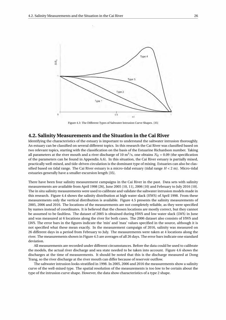
4.2. Salinity Measurements and the Situation in the Cai River 26
Figure 4.3: The Different Types of Saltwater Intrusion Curve Shapes. [35]
4.2. Salinity Measurements and the Situation in the Cai RiverIdentifying the characteristics of the estuary is important to understand the saltwater intrusion thoroughly.An estuary can be classified on several different topics. In this research the Cai River was classified based ontwo relevant topics, starting with the classification on the basis of the Estuarine Richardson number. Takingall parameters at the river mouth and a river discharge of 10 m3/s, one obtains NR = 0.09 (the specificationof the parameters can be found in Appendix A.6). In this situation, the Cai River estuary is partially mixed,practically well-mixed, and tide-driven circulation is the dominant type of mixing. Estuaries can also be clas-sified based on tidal range. The Cai River estuary is a micro-tidal estuary (tidal range H < 2 m). Micro-tidalestuaries generally have a smaller excursion length [35].
There have been four salinity measurement campaigns in the Cai River in the past. Data sets with salinitymeasurements are available from April 1998 [26], June 2005 [10, 11], 2006 [10] and February to July 2016 [10].The in situ salinity measurements were used to calibrate and validate the saltwater intrusion models made inthis research. Figure 4.4 shows the salinity distribution at high water slack (HWS) of April 1998. From thesemeasurements only the vertical distribution is available. Figure 4.5 presents the salinity measurements of2005, 2006 and 2016. The locations of the measurements are not completely reliable, as they were specifiedby names instead of coordinates. It is believed that the chosen locations are mostly correct, but they cannotbe assumed to be faultless. The dataset of 2005 is obtained during HWS and low water slack (LWS) in Juneand was measured at 6 locations along the river for both cases. The 2006 dataset also consists of HWS andLWS. The error bars in the figures indicate the ’min’ and ’max’ values specified in the source, although it isnot specified what these mean exactly. In the measurement campaign of 2016, salinity was measured on26 different days in a period from February to July. The measurements were taken at 4 locations along theriver. The measurements shown in Figure 4.5 are averages of all 26 days. The error bars indicate one standarddeviation.
All measurements are recorded under different circumstances. Before the data could be used to calibratethe models, the actual river discharge and sea state needed to be taken into account. Figure 4.6 shows thedischarges at the time of measurements. It should be noted that this is the discharge measured at DongTrang, so the river discharge at the river mouth can differ because of reservoir outflow.
The saltwater intrusion looks stratified in 1998. In 2005, 2006 and 2016 the measurements show a salinitycurve of the well-mixed type. The spatial resolution of the measurements is too low to be certain about thetype of the intrusion curve shape. However, the data show characteristics of a type 2 shape.
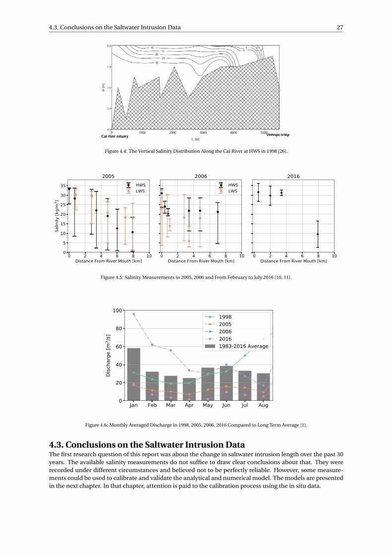
4.3. Conclusions on the Saltwater Intrusion Data 27
Figure 4.4: The Vertical Salinity Distribution Along the Cai River at HWS in 1998 [26].
0 2 4 6 8 10Distance From River Mouth [km]
0
5
10
15
20
25
30
35
Salin
ity [k
g/m
3 ]
2005HWSLWS
0 2 4 6 8 10Distance From River Mouth [km]
2006HWSLWS
0 2 4 6 8 10Distance From River Mouth [km]
2016
Figure 4.5: Salinity Measurements in 2005, 2006 and From February to July 2016 [10, 11].
Jan Feb Mar Apr May Jun Jul Aug0
20
40
60
80
100
Disc
harg
e [m
3 /s]
19982005200620161983-2016 Average
Figure 4.6: Monthly Averaged Discharge in 1998, 2005, 2006, 2016 Compared to Long Term Average [1].
4.3. Conclusions on the Saltwater Intrusion DataThe first research question of this report was about the change in saltwater intrusion length over the past 30years. The available salinity measurements do not suffice to draw clear conclusions about that. They wererecorded under different circumstances and believed not to be perfectly reliable. However, some measure-ments could be used to calibrate and validate the analytical and numerical model. The models are presentedin the next chapter. In that chapter, attention is paid to the calibration process using the in situ data.
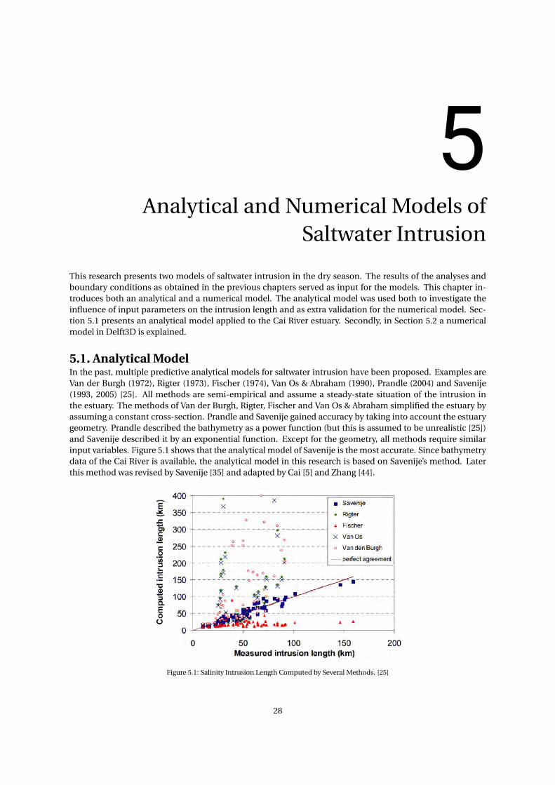
5Analytical and Numerical Models of
Saltwater Intrusion
This research presents two models of saltwater intrusion in the dry season. The results of the analyses andboundary conditions as obtained in the previous chapters served as input for the models. This chapter in-troduces both an analytical and a numerical model. The analytical model was used both to investigate theinfluence of input parameters on the intrusion length and as extra validation for the numerical model. Sec-tion 5.1 presents an analytical model applied to the Cai River estuary. Secondly, in Section 5.2 a numericalmodel in Delft3D is explained.
5.1. Analytical ModelIn the past, multiple predictive analytical models for saltwater intrusion have been proposed. Examples areVan der Burgh (1972), Rigter (1973), Fischer (1974), Van Os & Abraham (1990), Prandle (2004) and Savenije(1993, 2005) [25]. All methods are semi-empirical and assume a steady-state situation of the intrusion inthe estuary. The methods of Van der Burgh, Rigter, Fischer and Van Os & Abraham simplified the estuary byassuming a constant cross-section. Prandle and Savenije gained accuracy by taking into account the estuarygeometry. Prandle described the bathymetry as a power function (but this is assumed to be unrealistic [25])and Savenije described it by an exponential function. Except for the geometry, all methods require similarinput variables. Figure 5.1 shows that the analytical model of Savenije is the most accurate. Since bathymetrydata of the Cai River is available, the analytical model in this research is based on Savenije’s method. Laterthis method was revised by Savenije [35] and adapted by Cai [5] and Zhang [44].
Figure 5.1: Salinity Intrusion Length Computed by Several Methods. [25]
28
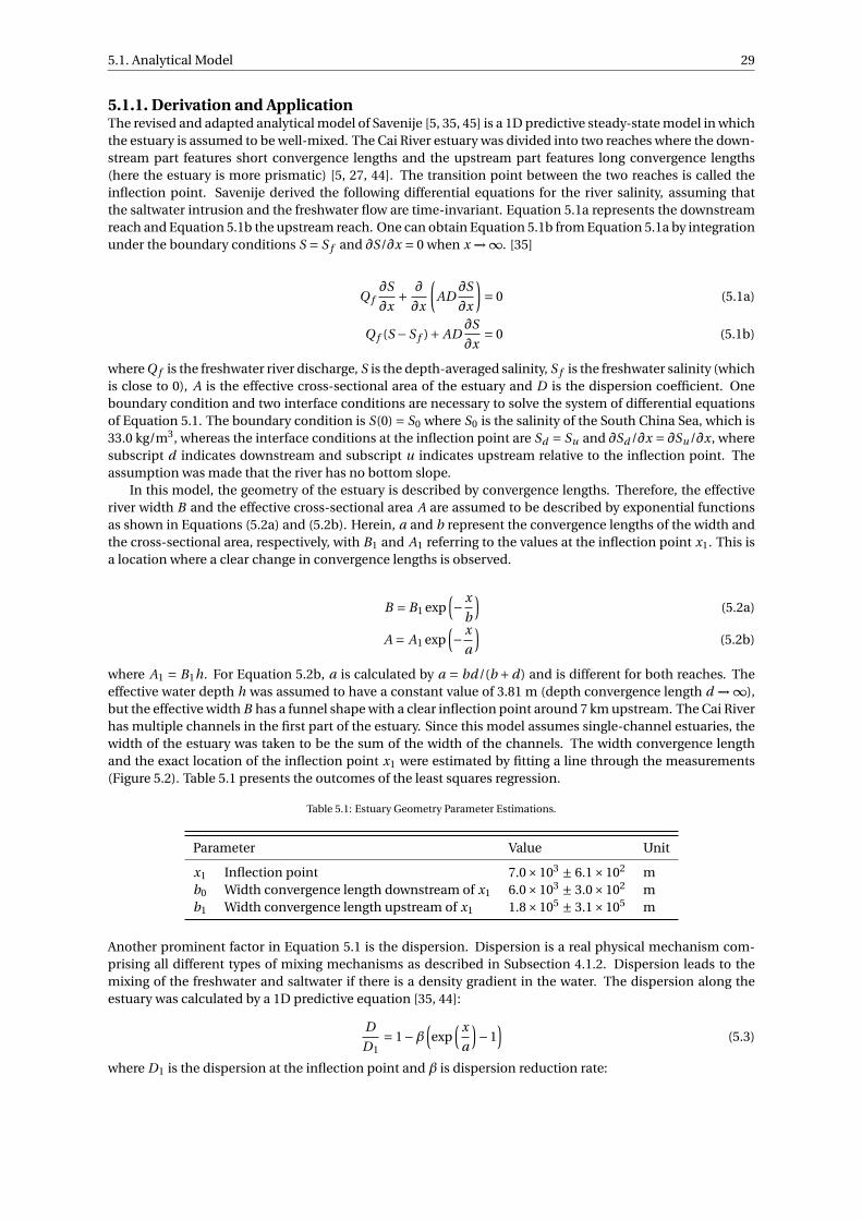
5.1. Analytical Model 29
5.1.1. Derivation and ApplicationThe revised and adapted analytical model of Savenije [5, 35, 45] is a 1D predictive steady-state model in whichthe estuary is assumed to be well-mixed. The Cai River estuary was divided into two reaches where the down-stream part features short convergence lengths and the upstream part features long convergence lengths(here the estuary is more prismatic) [5, 27, 44]. The transition point between the two reaches is called theinflection point. Savenije derived the following differential equations for the river salinity, assuming thatthe saltwater intrusion and the freshwater flow are time-invariant. Equation 5.1a represents the downstreamreach and Equation 5.1b the upstream reach. One can obtain Equation 5.1b from Equation 5.1a by integrationunder the boundary conditions S = S f and ∂S/∂x = 0 when x −→∞. [35]
Q f∂S
∂x+ ∂
∂x
(AD
∂S
∂x
)= 0 (5.1a)
Q f (S −S f )+ AD∂S
∂x= 0 (5.1b)
where Q f is the freshwater river discharge, S is the depth-averaged salinity, S f is the freshwater salinity (whichis close to 0), A is the effective cross-sectional area of the estuary and D is the dispersion coefficient. Oneboundary condition and two interface conditions are necessary to solve the system of differential equationsof Equation 5.1. The boundary condition is S(0) = S0 where S0 is the salinity of the South China Sea, which is33.0 kg/m3, whereas the interface conditions at the inflection point are Sd = Su and ∂Sd /∂x = ∂Su/∂x, wheresubscript d indicates downstream and subscript u indicates upstream relative to the inflection point. Theassumption was made that the river has no bottom slope.
In this model, the geometry of the estuary is described by convergence lengths. Therefore, the effectiveriver width B and the effective cross-sectional area A are assumed to be described by exponential functionsas shown in Equations (5.2a) and (5.2b). Herein, a and b represent the convergence lengths of the width andthe cross-sectional area, respectively, with B1 and A1 referring to the values at the inflection point x1. This isa location where a clear change in convergence lengths is observed.
B = B1 exp(−x
b
)(5.2a)
A = A1 exp(− x
a
)(5.2b)
where A1 = B1h. For Equation 5.2b, a is calculated by a = bd/(b +d) and is different for both reaches. Theeffective water depth h was assumed to have a constant value of 3.81 m (depth convergence length d −→∞),but the effective width B has a funnel shape with a clear inflection point around 7 km upstream. The Cai Riverhas multiple channels in the first part of the estuary. Since this model assumes single-channel estuaries, thewidth of the estuary was taken to be the sum of the width of the channels. The width convergence lengthand the exact location of the inflection point x1 were estimated by fitting a line through the measurements(Figure 5.2). Table 5.1 presents the outcomes of the least squares regression.
Table 5.1: Estuary Geometry Parameter Estimations.
Parameter Value Unit
x1 Inflection point 7.0×10³ ± 6.1×10² mb0 Width convergence length downstream of x1 6.0×10³ ± 3.0×10² mb1 Width convergence length upstream of x1 1.8×10⁵ ± 3.1×10⁵ m
Another prominent factor in Equation 5.1 is the dispersion. Dispersion is a real physical mechanism com-prising all different types of mixing mechanisms as described in Subsection 4.1.2. Dispersion leads to themixing of the freshwater and saltwater if there is a density gradient in the water. The dispersion along theestuary was calculated by a 1D predictive equation [35, 44]:
D
D1= 1−β
(exp
( x
a
)−1
)(5.3)
where D1 is the dispersion at the inflection point and β is dispersion reduction rate:
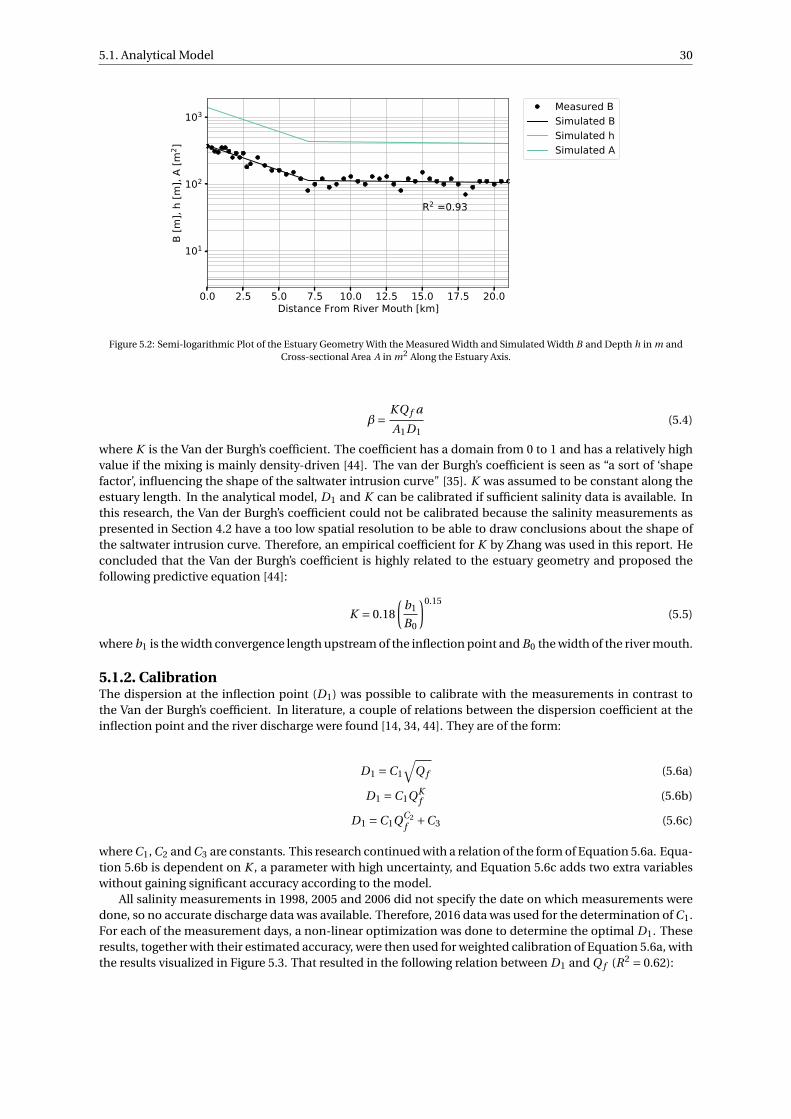
5.1. Analytical Model 30
0.0 2.5 5.0 7.5 10.0 12.5 15.0 17.5 20.0Distance From River Mouth [km]
101
102
103
B [m
], h
[m],
A [m
2 ]
R2 =0.93
Measured BSimulated BSimulated hSimulated A
Figure 5.2: Semi-logarithmic Plot of the Estuary Geometry With the Measured Width and Simulated Width B and Depth h in m andCross-sectional Area A in m2 Along the Estuary Axis.
β= KQ f a
A1D1(5.4)
where K is the Van der Burgh’s coefficient. The coefficient has a domain from 0 to 1 and has a relatively highvalue if the mixing is mainly density-driven [44]. The van der Burgh’s coefficient is seen as “a sort of ‘shapefactor’, influencing the shape of the saltwater intrusion curve" [35]. K was assumed to be constant along theestuary length. In the analytical model, D1 and K can be calibrated if sufficient salinity data is available. Inthis research, the Van der Burgh’s coefficient could not be calibrated because the salinity measurements aspresented in Section 4.2 have a too low spatial resolution to be able to draw conclusions about the shape ofthe saltwater intrusion curve. Therefore, an empirical coefficient for K by Zhang was used in this report. Heconcluded that the Van der Burgh’s coefficient is highly related to the estuary geometry and proposed thefollowing predictive equation [44]:
K = 0.18
(b1
B0
)0.15
(5.5)
where b1 is the width convergence length upstream of the inflection point and B0 the width of the river mouth.
5.1.2. CalibrationThe dispersion at the inflection point (D1) was possible to calibrate with the measurements in contrast tothe Van der Burgh’s coefficient. In literature, a couple of relations between the dispersion coefficient at theinflection point and the river discharge were found [14, 34, 44]. They are of the form:
D1 =C1
√Q f (5.6a)
D1 =C1QKf (5.6b)
D1 =C1QC2f +C3 (5.6c)
where C1, C2 and C3 are constants. This research continued with a relation of the form of Equation 5.6a. Equa-tion 5.6b is dependent on K , a parameter with high uncertainty, and Equation 5.6c adds two extra variableswithout gaining significant accuracy according to the model.
All salinity measurements in 1998, 2005 and 2006 did not specify the date on which measurements weredone, so no accurate discharge data was available. Therefore, 2016 data was used for the determination of C1.For each of the measurement days, a non-linear optimization was done to determine the optimal D1. Theseresults, together with their estimated accuracy, were then used for weighted calibration of Equation 5.6a, withthe results visualized in Figure 5.3. That resulted in the following relation between D1 and Q f (R2 = 0.62):
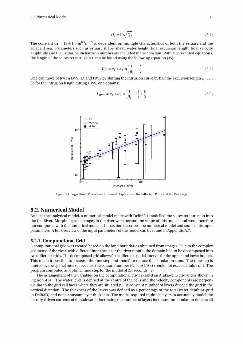
5.2. Numerical Model 31
D1 = 19√
Q f (5.7)
The constant C1 = 19± 1.6 m0.5s−0.5 is dependent on multiple characteristics of both the estuary and theadjacent sea. Parameters such as estuary shape, mean water height, tidal excursion length, tidal velocityamplitude and the Estuarine Richardson number are included in the constant. With all presented equations,the length of the saltwater intrusion L can be found using the following equation [35]:
LTA = x1 +a1 ln
(1
β1+1
)(5.8)
One can move between LWS, TA and HWS by shifting the intrusion curve by half the excursion length E [35].So for the intrusion length during HWS, one obtains:
LHWS = x1 +a1 ln
(1
β1+1
)+ E
2(5.9)
100 101
Discharge [m3/s]
101
102
Optim
ized
D 1 [m
2 /s]
Fit90% CIdata
Figure 5.3: Logarithmic Plot of the Optimized Dispersion at the Inflection Point and the Discharge
5.2. Numerical ModelBesides the analytical model, a numerical model made with Delft3D4 modelled the saltwater intrusion intothe Cai River. Morphological changes in the river were beyond the scope of this project and were thereforenot computed with the numerical model. This section describes the numerical model and some of its inputparameters. A full overview of the input parameters of the model can be found in Appendix A.7.
5.2.1. Computational GridA computational grid was created based on the land boundaries obtained from images. Due to the complexgeometry of the river, with different branches near the river mouth, the domain had to be decomposed intotwo different grids. The decomposed grid allows for a different spatial interval for the upper and lower branch.This made it possible to increase the timestep and therefore reduce the simulation time. The timestep islimited by the spatial interval because the courant number (C = u∆t/∆x) should not exceed a value of 1. Theprogram computed an optimal time step for the model of 2.4 seconds. [9]
The arrangement of the variables on the computational grid is called an Arakawa C-grid and is shown inFigure 5.4 [4]. The water level is defined at the centre of the cells and the velocity components are perpen-dicular to the grid cell faces where they are situated [9]. A constant number of layers divided the grid in thevertical direction. The thickness of the layers was defined as a percentage of the total water depth (σ-gridin Delft3D) and not a constant layer thickness. The model required multiple layers to accurately model thedensity-driven currents of the saltwater. Increasing the number of layers increases the simulation time, as all
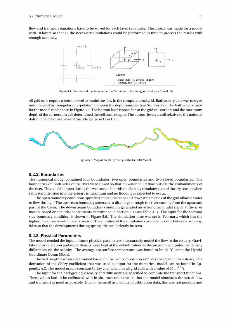
5.2. Numerical Model 32
flow and transport equations have to be solved for each layer separately. The choice was made for a modelwith 10 layers so that all the necessary simulations could be performed in time to process the results withenough accuracy.
Figure 5.4: Overview of the Arrangement of Variables in the Staggered Arakawa C-grid. [9]
All grid cells require a bottom level to model the flow in the computational grid. Bathymetry data was mergedonto the grid by triangular interpolation between the depth samples (see Section 3.2). The bathymetry usedfor the model can be seen in Figure 5.5. The bottom level is specified at the grid cell corners and the maximumdepth of the corners of a cell determined the cell centre depth. The bottom levels are all relative to the nationaldatum, the mean sea level of the tide gauge in Hon Dau.
Figure 5.5: Map of the Bathymetry of the Delft3D Model.
5.2.2. BoundariesThe numerical model contained four boundaries, two open boundaries and two closed boundaries. Theboundaries on both sides of the river were closed so that no water could flow outside the embankments ofthe river. This could happen during the wet season but this model only simulates part of the dry season whensaltwater intrusion into the estuary is maximum and no flooding is expected to occur.
The open boundary conditions specified at the upstream and downstream ends of the grid allowed waterto flow through. The upstream boundary generated a discharge through the river coming from the upstreampart of the basin. The downstream boundary condition generated an astronomical tidal signal at the rivermouth, based on the tidal constituents determined in Section 3.1 (see Table 3.1). The input for the seawardside boundary condition is shown in Figure 5.6. The simulation time was set in February, which has thehighest mean sea level of the dry season. The duration of the simulation covered one cycle between two neaptides so that the developments during spring tide could clearly be seen.
5.2.3. Physical ParametersThe model needed the input of some physical parameters to accurately model the flow in the estuary. Gravi-tational acceleration and water density were kept at the default values as the program computes the densitydifferences via the salinity. The average sea surface temperature was found to be 25 ◦C using the HybridCoordinate Ocean Model.
The bed roughness was determined based on the bed composition samples collected in the estuary. Thederivation of the Chézy coefficient that was used as input for the numerical model can be found in Ap-pendix A.2. The model used a constant Chézy coefficient for all grid cells with a value of 65 m0.5/s.
The input for the background viscosity and diffusivity are specified to compute the transport functions.These values had to be calibrated with in situ measurements so that the model simulates the actual flowand transport as good as possible. Due to the small availability of calibration data, this was not possible and
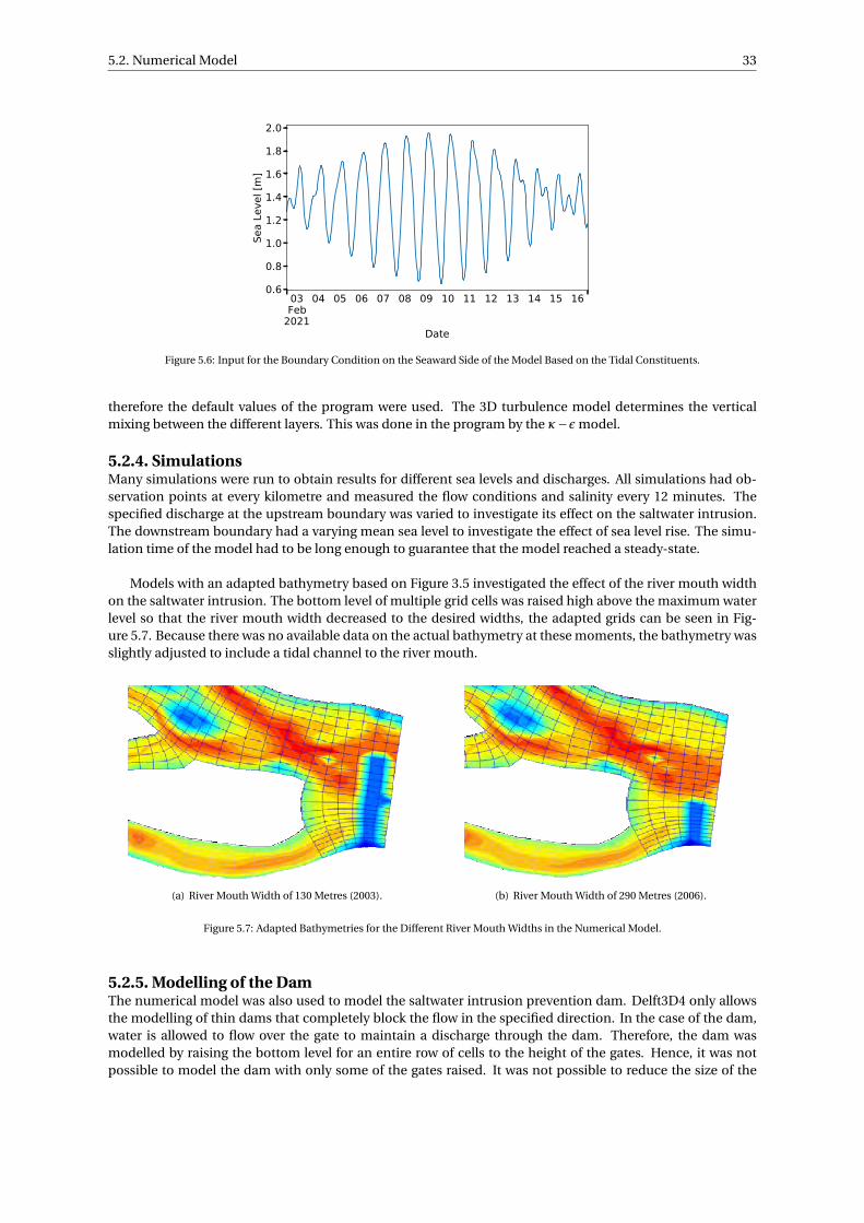
5.2. Numerical Model 33
03Feb
2021
04 05 06 07 08 09 10 11 12 13 14 15 16
Date
0.6
0.8
1.0
1.2
1.4
1.6
1.8
2.0
Sea
Leve
l [m
]
Figure 5.6: Input for the Boundary Condition on the Seaward Side of the Model Based on the Tidal Constituents.
therefore the default values of the program were used. The 3D turbulence model determines the verticalmixing between the different layers. This was done in the program by the κ−ε model.
5.2.4. SimulationsMany simulations were run to obtain results for different sea levels and discharges. All simulations had ob-servation points at every kilometre and measured the flow conditions and salinity every 12 minutes. Thespecified discharge at the upstream boundary was varied to investigate its effect on the saltwater intrusion.The downstream boundary had a varying mean sea level to investigate the effect of sea level rise. The simu-lation time of the model had to be long enough to guarantee that the model reached a steady-state.
Models with an adapted bathymetry based on Figure 3.5 investigated the effect of the river mouth widthon the saltwater intrusion. The bottom level of multiple grid cells was raised high above the maximum waterlevel so that the river mouth width decreased to the desired widths, the adapted grids can be seen in Fig-ure 5.7. Because there was no available data on the actual bathymetry at these moments, the bathymetry wasslightly adjusted to include a tidal channel to the river mouth.
(a) River Mouth Width of 130 Metres (2003). (b) River Mouth Width of 290 Metres (2006).
Figure 5.7: Adapted Bathymetries for the Different River Mouth Widths in the Numerical Model.
5.2.5. Modelling of the DamThe numerical model was also used to model the saltwater intrusion prevention dam. Delft3D4 only allowsthe modelling of thin dams that completely block the flow in the specified direction. In the case of the dam,water is allowed to flow over the gate to maintain a discharge through the dam. Therefore, the dam wasmodelled by raising the bottom level for an entire row of cells to the height of the gates. Hence, it was notpossible to model the dam with only some of the gates raised. It was not possible to reduce the size of the
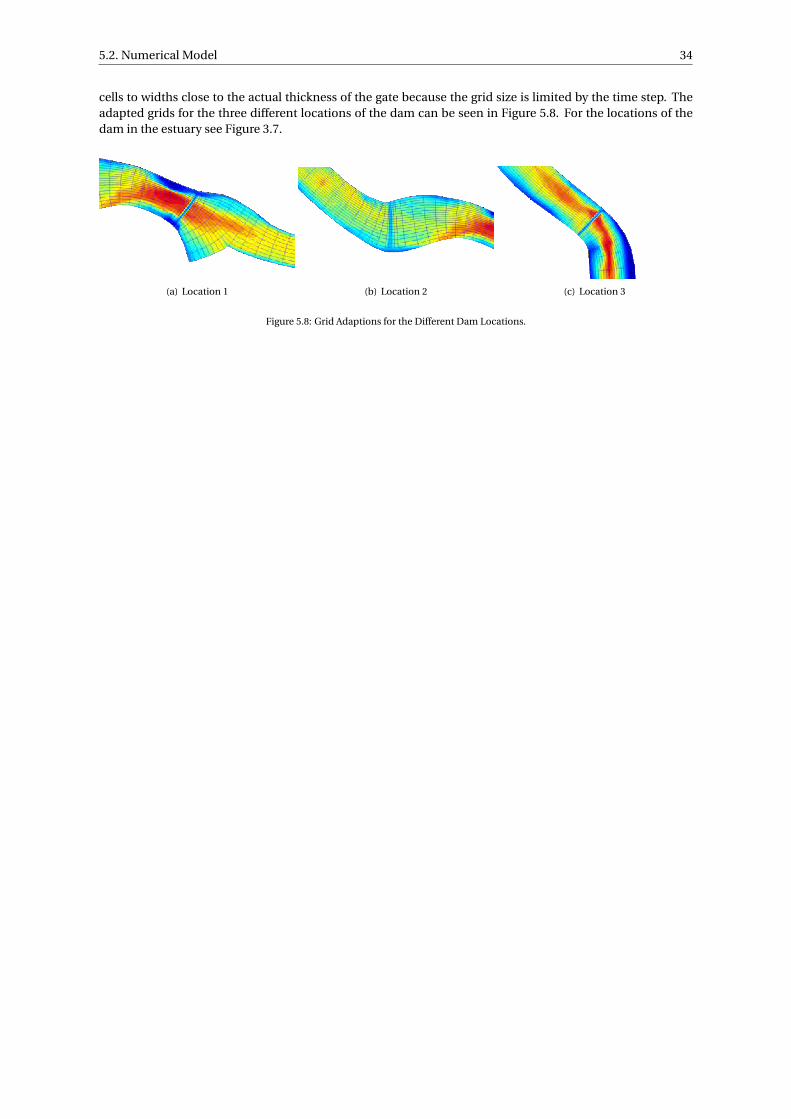
5.2. Numerical Model 34
cells to widths close to the actual thickness of the gate because the grid size is limited by the time step. Theadapted grids for the three different locations of the dam can be seen in Figure 5.8. For the locations of thedam in the estuary see Figure 3.7.
(a) Location 1 (b) Location 2 (c) Location 3
Figure 5.8: Grid Adaptions for the Different Dam Locations.
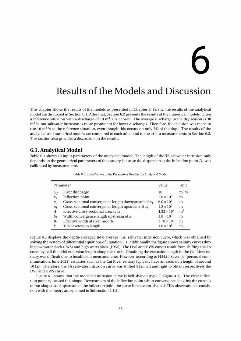
6Results of the Models and Discussion
This chapter shows the results of the models as presented in Chapter 5. Firstly, the results of the analyticalmodel are discussed in Section 6.1. After that, Section 6.2 presents the results of the numerical models. Oftena reference situation with a discharge of 10 m3/s is chosen. The average discharge in the dry season is 30m3/s, but saltwater intrusion is more prominent for lower discharges. Therefore, the decision was made touse 10 m3/s as the reference situation, even though this occurs on only 7% of the days. The results of theanalytical and numerical models are compared to each other and to the in situ measurements in Section 6.3.This section also provides a discussion on the results.
6.1. Analytical ModelTable 6.1 shows all input parameters of the analytical model. The length of the TA saltwater intrusion onlydepends on the geometrical parameters of the estuary, because the dispersion at the inflection point D1 wascalibrated by measurements.
Table 6.1: Initial Values of the Parameters Used in the Analytical Model.
Parameter Value Unit
Q f River discharge 10 m3/sx1 Inflection point 7.0×10³ ma0 Cross-sectional convergence length downstream of x1 6.0×10³ ma1 Cross-sectional convergence length upstream of x1 1.8×10⁵ mA1 Effective cross-sectional area at x1 4.33×10² m2
b1 Width convergence length upstream of x1 1.8×10⁵ mB0 Effective width at river mouth 3.70×10² mE Tidal excursion length 1.0×10⁴ m
Figure 6.1 displays the depth-averaged tidal average (TA) saltwater intrusion curve, which was obtained bysolving the system of differential equations of Equation 5.1. Additionally, the figure shows salinity curves dur-ing low water slack (LWS) and high water slack (HWS). The LWS and HWS curves result from shifting the TAcurve by half the tidal excursion length along the x-axis. Obtaining the excursion length in the Cai River es-tuary was difficult due to insufficient measurements. However, according to H.H.G. Savenije (personal com-munication, June 2021) estuaries such as the Cai River estuary typically have an excursion length of around10 km. Therefore, the TA saltwater intrusion curve was shifted 5 km left and right to obtain respectively theLWS and HWS curve.
Figure 6.1 shows that the modelled intrusion curve is bell-shaped (type 2, Figure 4.3). The clear inflec-tion point x1 caused this shape. Downstream of the inflection point (short convergence lengths) the curve isdome-shaped and upstream of the inflection point the curve is recession-shaped. This observation is consis-tent with the theory as explained in Subsection 4.1.3.
35
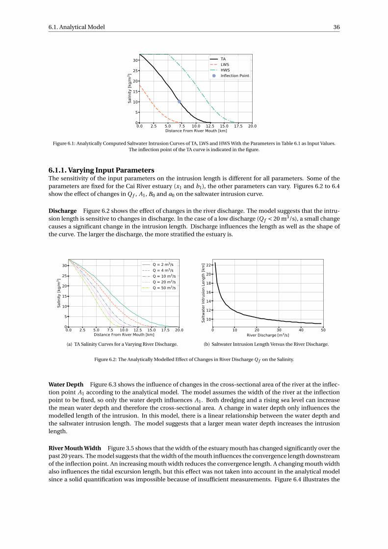
6.1. Analytical Model 36
0.0 2.5 5.0 7.5 10.0 12.5 15.0 17.5 20.0Distance From River Mouth [km]
0
5
10
15
20
25
30
Salin
ity [k
g/m
3 ]
TALWSHWSInflection Point
Figure 6.1: Analytically Computed Saltwater Intrusion Curves of TA, LWS and HWS With the Parameters in Table 6.1 as Input Values.The inflection point of the TA curve is indicated in the figure.
6.1.1. Varying Input ParametersThe sensitivity of the input parameters on the intrusion length is different for all parameters. Some of theparameters are fixed for the Cai River estuary (x1 and b1), the other parameters can vary. Figures 6.2 to 6.4show the effect of changes in Q f , A1, B0 and a0 on the saltwater intrusion curve.
Discharge Figure 6.2 shows the effect of changes in the river discharge. The model suggests that the intru-sion length is sensitive to changes in discharge. In the case of a low discharge (Q f < 20 m3/s), a small changecauses a significant change in the intrusion length. Discharge influences the length as well as the shape ofthe curve. The larger the discharge, the more stratified the estuary is.
0.0 2.5 5.0 7.5 10.0 12.5 15.0 17.5 20.0Distance From River Mouth [km]
0
5
10
15
20
25
30
Salin
ity [k
g/m
3 ]
Q = 2 m3/sQ = 4 m3/sQ = 10 m3/sQ = 20 m3/sQ = 50 m3/s
(a) TA Salinity Curves for a Varying River Discharge.
0 10 20 30 40 50River Discharge [m3/s]
10
12
14
16
18
20
22
Saltw
ater
Intru
sion
Leng
th [k
m]
(b) Saltwater Intrusion Length Versus the River Discharge.
Figure 6.2: The Analytically Modelled Effect of Changes in River Discharge Q f on the Salinity.
Water Depth Figure 6.3 shows the influence of changes in the cross-sectional area of the river at the inflec-tion point A1 according to the analytical model. The model assumes the width of the river at the inflectionpoint to be fixed, so only the water depth influences A1. Both dredging and a rising sea level can increasethe mean water depth and therefore the cross-sectional area. A change in water depth only influences themodelled length of the intrusion. In this model, there is a linear relationship between the water depth andthe saltwater intrusion length. The model suggests that a larger mean water depth increases the intrusionlength.
River Mouth Width Figure 3.5 shows that the width of the estuary mouth has changed significantly over thepast 20 years. The model suggests that the width of the mouth influences the convergence length downstreamof the inflection point. An increasing mouth width reduces the convergence length. A changing mouth widthalso influences the tidal excursion length, but this effect was not taken into account in the analytical modelsince a solid quantification was impossible because of insufficient measurements. Figure 6.4 illustrates the
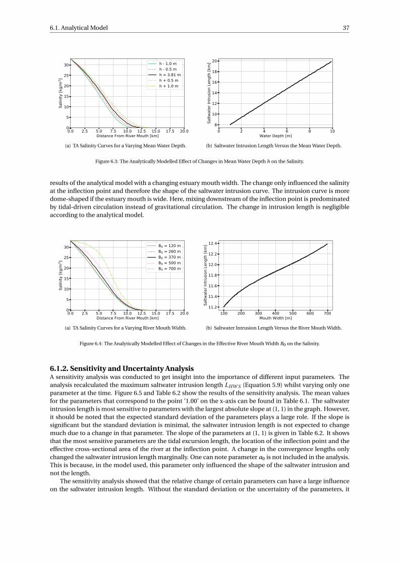
6.1. Analytical Model 37
0.0 2.5 5.0 7.5 10.0 12.5 15.0 17.5 20.0Distance From River Mouth [km]
0
5
10
15
20
25
30Sa
linity
[kg/
m3 ]
h - 1.0 mh - 0.5 mh = 3.81 mh + 0.5 mh + 1.0 m
(a) TA Salinity Curves for a Varying Mean Water Depth.
0 2 4 6 8 10Water Depth [m]
8
10
12
14
16
18
20
Saltw
ater
Intru
sion
Leng
th [k
m]
(b) Saltwater Intrusion Length Versus the Mean Water Depth.
Figure 6.3: The Analytically Modelled Effect of Changes in Mean Water Depth h on the Salinity.
results of the analytical model with a changing estuary mouth width. The change only influenced the salinityat the inflection point and therefore the shape of the saltwater intrusion curve. The intrusion curve is moredome-shaped if the estuary mouth is wide. Here, mixing downstream of the inflection point is predominatedby tidal-driven circulation instead of gravitational circulation. The change in intrusion length is negligibleaccording to the analytical model.
0.0 2.5 5.0 7.5 10.0 12.5 15.0 17.5 20.0Distance From River Mouth [km]
0
5
10
15
20
25
30
Salin
ity [k
g/m
3 ]
B0 = 120 mB0 = 260 mB0 = 370 mB0 = 500 mB0 = 700 m
(a) TA Salinity Curves for a Varying River Mouth Width.
100 200 300 400 500 600 700Mouth Width [m]
11.2
11.4
11.6
11.8
12.0
12.2
12.4
Saltw
ater
Intru
sion
Leng
th [k
m]
(b) Saltwater Intrusion Length Versus the River Mouth Width.
Figure 6.4: The Analytically Modelled Effect of Changes in the Effective River Mouth Width B0 on the Salinity.
6.1.2. Sensitivity and Uncertainty AnalysisA sensitivity analysis was conducted to get insight into the importance of different input parameters. Theanalysis recalculated the maximum saltwater intrusion length LHW S (Equation 5.9) whilst varying only oneparameter at the time. Figure 6.5 and Table 6.2 show the results of the sensitivity analysis. The mean valuesfor the parameters that correspond to the point ’1.00’ on the x-axis can be found in Table 6.1. The saltwaterintrusion length is most sensitive to parameters with the largest absolute slope at (1, 1) in the graph. However,it should be noted that the expected standard deviation of the parameters plays a large role. If the slope issignificant but the standard deviation is minimal, the saltwater intrusion length is not expected to changemuch due to a change in that parameter. The slope of the parameters at (1, 1) is given in Table 6.2. It showsthat the most sensitive parameters are the tidal excursion length, the location of the inflection point and theeffective cross-sectional area of the river at the inflection point. A change in the convergence lengths onlychanged the saltwater intrusion length marginally. One can note parameter a0 is not included in the analysis.This is because, in the model used, this parameter only influenced the shape of the saltwater intrusion andnot the length.
The sensitivity analysis showed that the relative change of certain parameters can have a large influenceon the saltwater intrusion length. Without the standard deviation or the uncertainty of the parameters, it
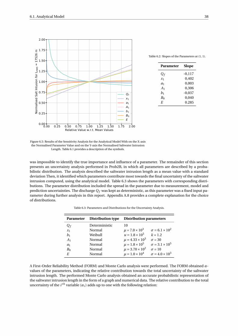
6.1. Analytical Model 38
0.00 0.25 0.50 0.75 1.00 1.25 1.50 1.75 2.00Relative Value w.r.t. Mean Values
0.00
0.25
0.50
0.75
1.00
1.25
1.50
1.75
2.00No
rmal
ised
Salt
Intu
sion
for L
HW
S = 1
7526
m
Qf
x1a1A1b1B0E
Figure 6.5: Results of the Sensitivity Analysis for the Analytical Model With on the X-axisthe Normalised Parameter Value and on the Y-axis the Normalised Saltwater Intrusion
Length. Table 6.1 provides a description of the symbols.
Table 6.2: Slopes of the Parameters at (1, 1).
Parameter Slope
Q f -0,117x1 0,402a1 0,003A1 0,306b1 -0,037B0 0,040E 0.285
was impossible to identify the true importance and influence of a parameter. The remainder of this sectionpresents an uncertainty analysis performed in Prob2B, in which all parameters are described by a proba-bilistic distribution. The analysis described the saltwater intrusion length as a mean value with a standarddeviation Then, it identified which parameters contribute most towards the final uncertainty of the saltwaterintrusion computed, using the analytical model. Table 6.3 shows the parameters with corresponding distri-butions. The parameter distribution included the spread in the parameter due to measurement, model andprediction uncertainties. The discharge Q f was kept as deterministic, as this parameter was a fixed input pa-rameter during further analysis in this report. Appendix A.8 provides a complete explanation for the choiceof distributions.
Table 6.3: Parameters and Distributions for the Uncertainty Analysis.
Parameter Distribution type Distribution parameters
Q f Deterministic 10x1 Normal µ = 7.0×10³ σ= 6.1×10²
b1 Weibull u = 1.8×10⁵ k = 1.2A1 Normal µ= 4.33×10³ σ = 30a1 Normal µ= 1.8×10⁵ σ= 3.1×10⁵
B0 Normal µ= 3.70×10² σ = 10E Normal µ= 1.0×10⁴ σ= 4.0×10³
A First-Order Reliability Method (FORM) and Monte Carlo analysis were performed. The FORM obtained α-values of the parameters, indicating the relative contribution towards the total uncertainty of the saltwaterintrusion length. The performed Monte Carlo analysis obtained an accurate probabilistic representation ofthe saltwater intrusion length in the form of a graph and numerical data. The relative contribution to the totaluncertainty of the i th variable (αi ) adds up to one with the following relation:
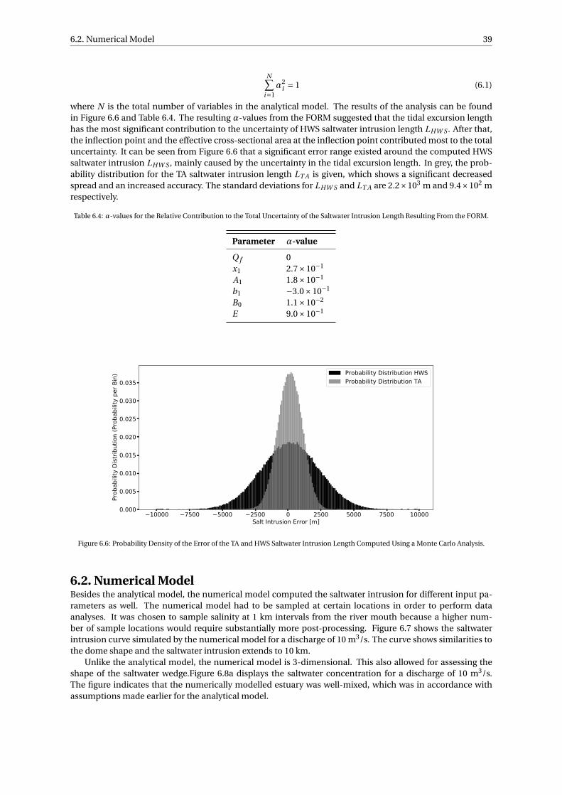
6.2. Numerical Model 39
N∑i=1
α2i = 1 (6.1)
where N is the total number of variables in the analytical model. The results of the analysis can be foundin Figure 6.6 and Table 6.4. The resulting α-values from the FORM suggested that the tidal excursion lengthhas the most significant contribution to the uncertainty of HWS saltwater intrusion length LHW S . After that,the inflection point and the effective cross-sectional area at the inflection point contributed most to the totaluncertainty. It can be seen from Figure 6.6 that a significant error range existed around the computed HWSsaltwater intrusion LHW S , mainly caused by the uncertainty in the tidal excursion length. In grey, the prob-ability distribution for the TA saltwater intrusion length LT A is given, which shows a significant decreasedspread and an increased accuracy. The standard deviations for LHW S and LT A are 2.2×10³ m and 9.4×10² mrespectively.
Table 6.4: α-values for the Relative Contribution to the Total Uncertainty of the Saltwater Intrusion Length Resulting From the FORM.
Parameter α-value
Q f 0x1 2.7×10⁻¹
A1 1.8×10⁻¹
b1 −3.0×10⁻¹
B0 1.1×10⁻²
E 9.0×10⁻¹
10000 7500 5000 2500 0 2500 5000 7500 10000Salt Intrusion Error [m]
0.000
0.005
0.010
0.015
0.020
0.025
0.030
0.035
Prob
abilit
y Di
strib
utio
n (P
roba
bilit
y pe
r Bin
) Probability Distribution HWSProbability Distribution TA
Figure 6.6: Probability Density of the Error of the TA and HWS Saltwater Intrusion Length Computed Using a Monte Carlo Analysis.
6.2. Numerical ModelBesides the analytical model, the numerical model computed the saltwater intrusion for different input pa-rameters as well. The numerical model had to be sampled at certain locations in order to perform dataanalyses. It was chosen to sample salinity at 1 km intervals from the river mouth because a higher num-ber of sample locations would require substantially more post-processing. Figure 6.7 shows the saltwaterintrusion curve simulated by the numerical model for a discharge of 10 m3/s. The curve shows similarities tothe dome shape and the saltwater intrusion extends to 10 km.
Unlike the analytical model, the numerical model is 3-dimensional. This also allowed for assessing theshape of the saltwater wedge.Figure 6.8a displays the saltwater concentration for a discharge of 10 m3/s.The figure indicates that the numerically modelled estuary was well-mixed, which was in accordance withassumptions made earlier for the analytical model.
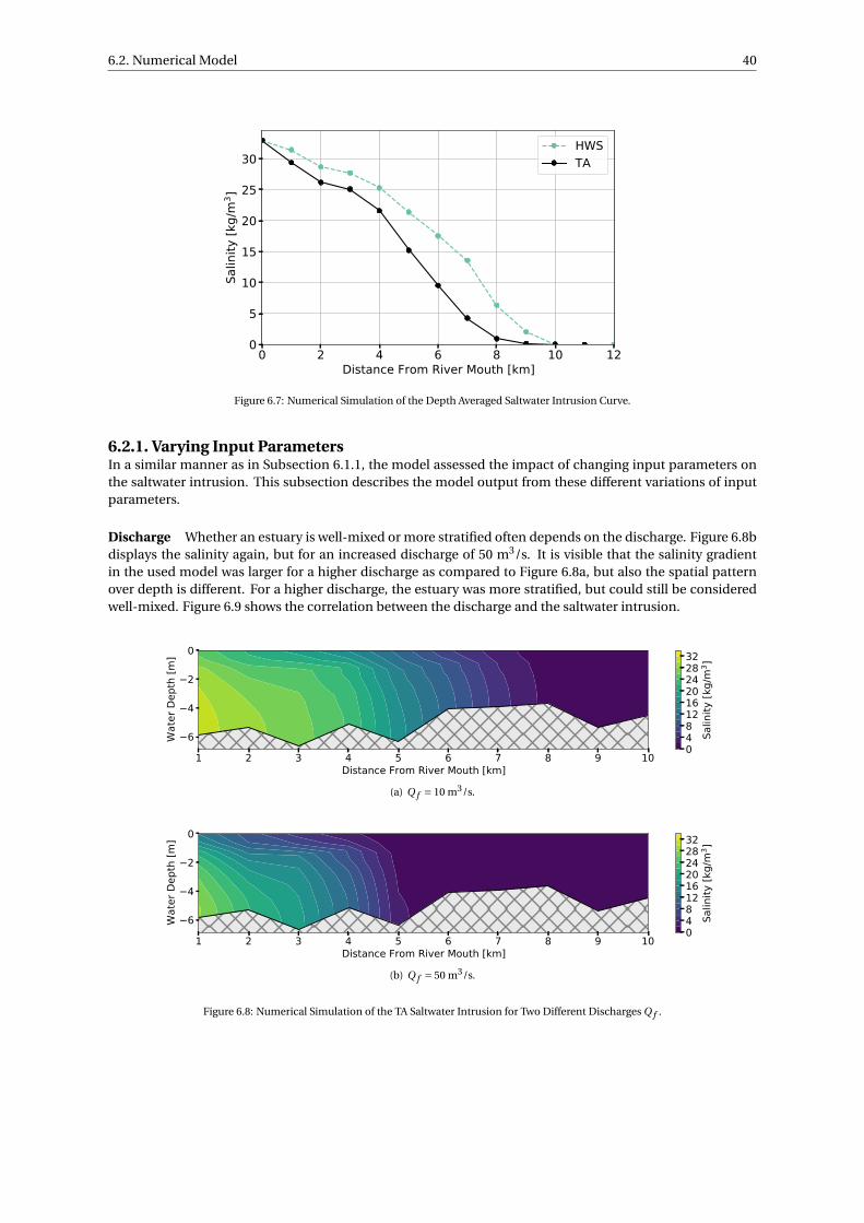
6.2. Numerical Model 40
0 2 4 6 8 10 12Distance From River Mouth [km]
0
5
10
15
20
25
30
Salin
ity [k
g/m
3 ]
HWSTA
Figure 6.7: Numerical Simulation of the Depth Averaged Saltwater Intrusion Curve.
6.2.1. Varying Input ParametersIn a similar manner as in Subsection 6.1.1, the model assessed the impact of changing input parameters onthe saltwater intrusion. This subsection describes the model output from these different variations of inputparameters.
Discharge Whether an estuary is well-mixed or more stratified often depends on the discharge. Figure 6.8bdisplays the salinity again, but for an increased discharge of 50 m3/s. It is visible that the salinity gradientin the used model was larger for a higher discharge as compared to Figure 6.8a, but also the spatial patternover depth is different. For a higher discharge, the estuary was more stratified, but could still be consideredwell-mixed. Figure 6.9 shows the correlation between the discharge and the saltwater intrusion.
1 2 3 4 5 6 7 8 9 10Distance From River Mouth [km]
6
4
2
0
Wat
er D
epth
[m]
048121620242832
Salin
ity [k
g/m
3 ]
(a) Q f = 10 m3/s.
1 2 3 4 5 6 7 8 9 10Distance From River Mouth [km]
6
4
2
0
Wat
er D
epth
[m]
048121620242832
Salin
ity [k
g/m
3 ]
(b) Q f = 50 m3/s.
Figure 6.8: Numerical Simulation of the TA Saltwater Intrusion for Two Different Discharges Q f .
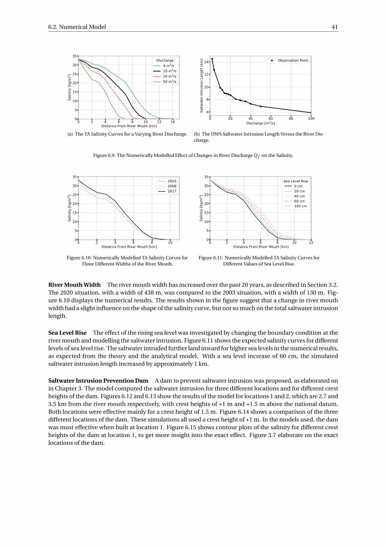
6.2. Numerical Model 41
0 2 4 6 8 10 12 14Distance From River Mouth [km]
0
5
10
15
20
25
30
35
Salin
ity [k
g/m
3 ]
Discharge4 m3/s10 m3/s20 m3/s50 m3/s
(a) The TA Salinity Curves for a Varying River Discharge.
0 20 40 60 80 100Discharge [m3/s]
6
8
10
12
14
Saltw
ater
Intru
sion
Leng
th [k
m] Observation Point
(b) The HWS Saltwater Intrusion Length Versus the River Dis-charge.
Figure 6.9: The Numerically Modelled Effect of Changes in River Discharge Q f on the Salinity.
0 2 4 6 8 10Distance From River Mouth [km]
0
5
10
15
20
25
30
35
Salin
ity [k
g/m
3 ]
200320062017
Figure 6.10: Numerically Modelled TA Salinity Curves forThree Different Widths of the River Mouth.
0 2 4 6 8 10 12Distance From River Mouth [km]
0
5
10
15
20
25
30
35
Salin
ity [k
g/m
3 ]
Sea Level Rise0 cm20 cm40 cm60 cm100 cm
Figure 6.11: Numerically Modelled TA Salinity Curves forDifferent Values of Sea Level Rise.
River Mouth Width The river mouth width has increased over the past 20 years, as described in Section 3.2.The 2020 situation, with a width of 438 m, was compared to the 2003 situation, with a width of 130 m. Fig-ure 6.10 displays the numerical results. The results shown in the figure suggest that a change in river mouthwidth had a slight influence on the shape of the salinity curve, but not so much on the total saltwater intrusionlength.
Sea Level Rise The effect of the rising sea level was investigated by changing the boundary condition at theriver mouth and modelling the saltwater intrusion. Figure 6.11 shows the expected salinity curves for differentlevels of sea level rise. The saltwater intruded further land inward for higher sea levels in the numerical results,as expected from the theory and the analytical model. With a sea level increase of 60 cm, the simulatedsaltwater intrusion length increased by approximately 1 km.
Saltwater Intrusion Prevention Dam A dam to prevent saltwater intrusion was proposed, as elaborated onin Chapter 3. The model computed the saltwater intrusion for three different locations and for different crestheights of the dam. Figures 6.12 and 6.13 show the results of the model for locations 1 and 2, which are 2.7 and3.5 km from the river mouth respectively, with crest heights of +1 m and +1.5 m above the national datum.Both locations were effective mainly for a crest height of 1.5 m. Figure 6.14 shows a comparison of the threedifferent locations of the dam. These simulations all used a crest height of +1 m. In the models used, the damwas most effective when built at location 1. Figure 6.15 shows contour plots of the salinity for different crestheights of the dam at location 1, to get more insight into the exact effect. Figure 3.7 elaborate on the exactlocations of the dam.
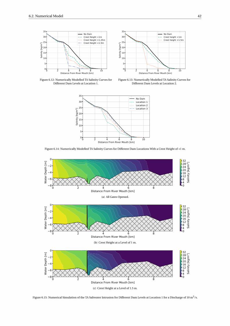
6.2. Numerical Model 42
0 2 4 6 8 10Distance From River Mouth [km]
0
5
10
15
20
25
30
35
Salin
ity [k
g/m
3 ]
No DamCrest Height +1mCrest Height +1.25mCrest Height +1.5m
Figure 6.12: Numerically Modelled TA Salinity Curves forDifferent Dam Levels at Location 1.
0 2 4 6 8 10Distance From River Mouth [km]
0
5
10
15
20
25
30
35
Salin
ity [k
g/m
3 ]
No DamCrest height +1mCrest height +1.5m
Figure 6.13: Numerically Modelled TA Salinity Curves forDifferent Dam Levels at Location 2.
0 2 4 6 8 10Distance From River Mouth [km]
0
5
10
15
20
25
30
35
Salin
ity [k
g/m
3 ]
No DamLocation 1Location 2Location 3
Figure 6.14: Numerically Modelled TA Salinity Curves for Different Dam Locations With a Crest Height of +1 m.
0 2 4 6 8Distance From River Mouth [km]
8
6
4
2
0
Wat
er D
epth
[m]
048121620242832
Salin
ity [k
g/m
3 ]
(a) All Gates Opened.
0 2 4 6 8Distance From River Mouth [km]
8
6
4
2
0
Wat
er D
epth
[m]
048121620242832
Salin
ity [k
g/m
3 ]
(b) Crest Height at a Level of 1 m.
0 2 4 6 8Distance From River Mouth [km]
8
6
4
2
0
Wat
er D
epth
[m]
048121620242832
Salin
ity [k
g/m
3 ]
(c) Crest Height at a Level of 1.5 m.
Figure 6.15: Numerical Simulation of the TA Saltwater Intrusion for Different Dam Levels at Location 1 for a Discharge of 10 m3/s.
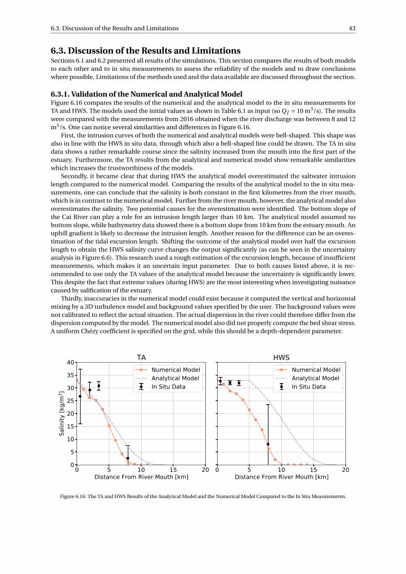
6.3. Discussion of the Results and Limitations 43
6.3. Discussion of the Results and LimitationsSections 6.1 and 6.2 presented all results of the simulations. This section compares the results of both modelsto each other and to in situ measurements to assess the reliability of the models and to draw conclusionswhere possible. Limitations of the methods used and the data available are discussed throughout the section.
6.3.1. Validation of the Numerical and Analytical ModelFigure 6.16 compares the results of the numerical and the analytical model to the in situ measurements forTA and HWS. The models used the initial values as shown in Table 6.1 as input (so Q f = 10 m3/s). The resultswere compared with the measurements from 2016 obtained when the river discharge was between 8 and 12m3/s. One can notice several similarities and differences in Figure 6.16.
First, the intrusion curves of both the numerical and analytical models were bell-shaped. This shape wasalso in line with the HWS in situ data, through which also a bell-shaped line could be drawn. The TA in situdata shows a rather remarkable course since the salinity increased from the mouth into the first part of theestuary. Furthermore, the TA results from the analytical and numerical model show remarkable similaritieswhich increases the trustworthiness of the models.
Secondly, it became clear that during HWS the analytical model overestimated the saltwater intrusionlength compared to the numerical model. Comparing the results of the analytical model to the in situ mea-surements, one can conclude that the salinity is both constant in the first kilometres from the river mouth,which is in contrast to the numerical model. Further from the river mouth, however, the analytical model alsooverestimates the salinity. Two potential causes for the overestimation were identified. The bottom slope ofthe Cai River can play a role for an intrusion length larger than 10 km. The analytical model assumed nobottom slope, while bathymetry data showed there is a bottom slope from 10 km from the estuary mouth. Anuphill gradient is likely to decrease the intrusion length. Another reason for the difference can be an overes-timation of the tidal excursion length. Shifting the outcome of the analytical model over half the excursionlength to obtain the HWS salinity curve changes the output significantly (as can be seen in the uncertaintyanalysis in Figure 6.6). This research used a rough estimation of the excursion length, because of insufficientmeasurements, which makes it an uncertain input parameter. Due to both causes listed above, it is rec-ommended to use only the TA values of the analytical model because the uncertainty is significantly lower.This despite the fact that extreme values (during HWS) are the most interesting when investigating nuisancecaused by salification of the estuary.
Thirdly, inaccuracies in the numerical model could exist because it computed the vertical and horizontalmixing by a 3D turbulence model and background values specified by the user. The background values werenot calibrated to reflect the actual situation. The actual dispersion in the river could therefore differ from thedispersion computed by the model. The numerical model also did not properly compute the bed shear stress.A uniform Chézy coefficient is specified on the grid, while this should be a depth-dependent parameter.
0 5 10 15 20Distance From River Mouth [km]
0
5
10
15
20
25
30
35
40
Salin
ity [k
g/m
3 ]
TANumerical ModelAnalytical ModelIn Situ Data
0 5 10 15 20Distance From River Mouth [km]
HWSNumerical ModelAnalytical ModelIn Situ Data
Figure 6.16: The TA and HWS Results of the Analytical Model and the Numerical Model Compared to the In Situ Measurements.
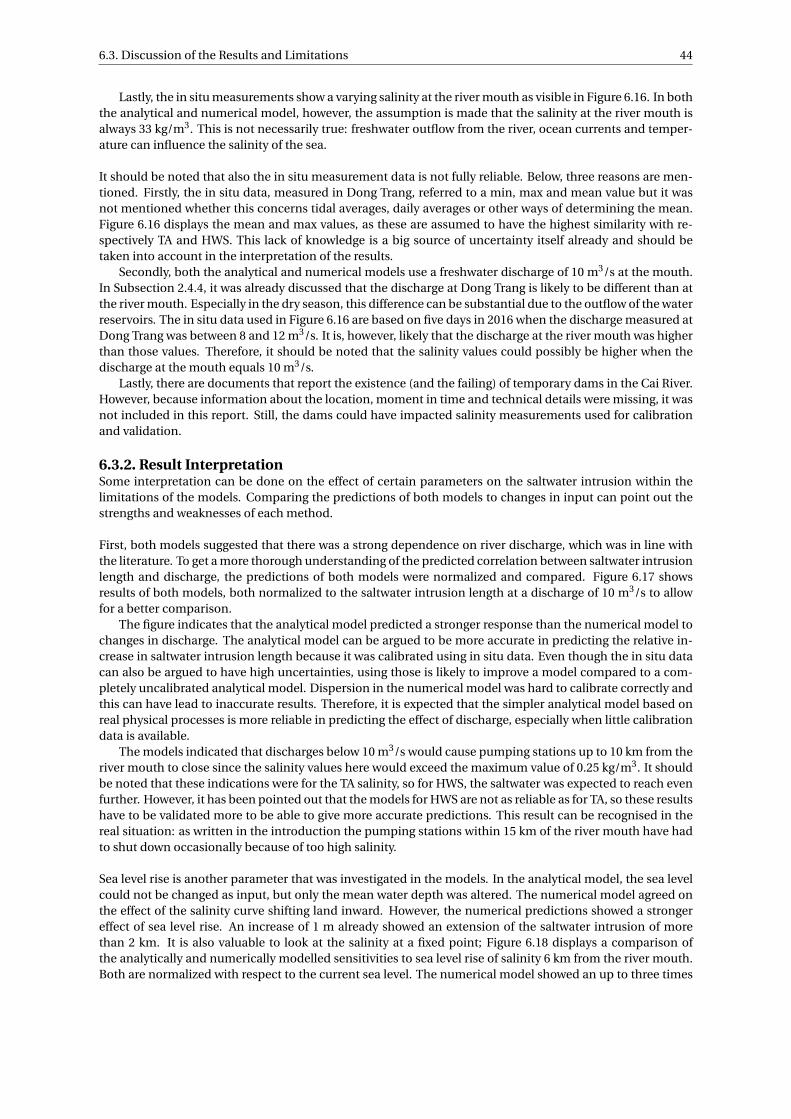
6.3. Discussion of the Results and Limitations 44
Lastly, the in situ measurements show a varying salinity at the river mouth as visible in Figure 6.16. In boththe analytical and numerical model, however, the assumption is made that the salinity at the river mouth isalways 33 kg/m3. This is not necessarily true: freshwater outflow from the river, ocean currents and temper-ature can influence the salinity of the sea.
It should be noted that also the in situ measurement data is not fully reliable. Below, three reasons are men-tioned. Firstly, the in situ data, measured in Dong Trang, referred to a min, max and mean value but it wasnot mentioned whether this concerns tidal averages, daily averages or other ways of determining the mean.Figure 6.16 displays the mean and max values, as these are assumed to have the highest similarity with re-spectively TA and HWS. This lack of knowledge is a big source of uncertainty itself already and should betaken into account in the interpretation of the results.
Secondly, both the analytical and numerical models use a freshwater discharge of 10 m3/s at the mouth.In Subsection 2.4.4, it was already discussed that the discharge at Dong Trang is likely to be different than atthe river mouth. Especially in the dry season, this difference can be substantial due to the outflow of the waterreservoirs. The in situ data used in Figure 6.16 are based on five days in 2016 when the discharge measured atDong Trang was between 8 and 12 m3/s. It is, however, likely that the discharge at the river mouth was higherthan those values. Therefore, it should be noted that the salinity values could possibly be higher when thedischarge at the mouth equals 10 m3/s.
Lastly, there are documents that report the existence (and the failing) of temporary dams in the Cai River.However, because information about the location, moment in time and technical details were missing, it wasnot included in this report. Still, the dams could have impacted salinity measurements used for calibrationand validation.
6.3.2. Result InterpretationSome interpretation can be done on the effect of certain parameters on the saltwater intrusion within thelimitations of the models. Comparing the predictions of both models to changes in input can point out thestrengths and weaknesses of each method.
First, both models suggested that there was a strong dependence on river discharge, which was in line withthe literature. To get a more thorough understanding of the predicted correlation between saltwater intrusionlength and discharge, the predictions of both models were normalized and compared. Figure 6.17 showsresults of both models, both normalized to the saltwater intrusion length at a discharge of 10 m3/s to allowfor a better comparison.
The figure indicates that the analytical model predicted a stronger response than the numerical model tochanges in discharge. The analytical model can be argued to be more accurate in predicting the relative in-crease in saltwater intrusion length because it was calibrated using in situ data. Even though the in situ datacan also be argued to have high uncertainties, using those is likely to improve a model compared to a com-pletely uncalibrated analytical model. Dispersion in the numerical model was hard to calibrate correctly andthis can have lead to inaccurate results. Therefore, it is expected that the simpler analytical model based onreal physical processes is more reliable in predicting the effect of discharge, especially when little calibrationdata is available.
The models indicated that discharges below 10 m3/s would cause pumping stations up to 10 km from theriver mouth to close since the salinity values here would exceed the maximum value of 0.25 kg/m3. It shouldbe noted that these indications were for the TA salinity, so for HWS, the saltwater was expected to reach evenfurther. However, it has been pointed out that the models for HWS are not as reliable as for TA, so these resultshave to be validated more to be able to give more accurate predictions. This result can be recognised in thereal situation: as written in the introduction the pumping stations within 15 km of the river mouth have hadto shut down occasionally because of too high salinity.
Sea level rise is another parameter that was investigated in the models. In the analytical model, the sea levelcould not be changed as input, but only the mean water depth was altered. The numerical model agreed onthe effect of the salinity curve shifting land inward. However, the numerical predictions showed a strongereffect of sea level rise. An increase of 1 m already showed an extension of the saltwater intrusion of morethan 2 km. It is also valuable to look at the salinity at a fixed point; Figure 6.18 displays a comparison ofthe analytically and numerically modelled sensitivities to sea level rise of salinity 6 km from the river mouth.Both are normalized with respect to the current sea level. The numerical model showed an up to three times
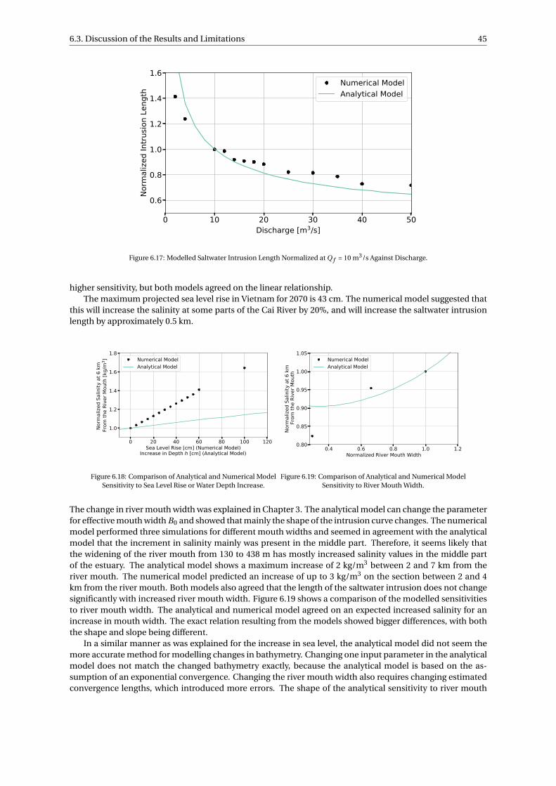
6.3. Discussion of the Results and Limitations 45
0 10 20 30 40 50Discharge [m3/s]
0.6
0.8
1.0
1.2
1.4
1.6
Norm
alize
d In
trusio
n Le
ngth
Numerical ModelAnalytical Model
Figure 6.17: Modelled Saltwater Intrusion Length Normalized at Q f = 10 m3/s Against Discharge.
higher sensitivity, but both models agreed on the linear relationship.The maximum projected sea level rise in Vietnam for 2070 is 43 cm. The numerical model suggested that
this will increase the salinity at some parts of the Cai River by 20%, and will increase the saltwater intrusionlength by approximately 0.5 km.
0 20 40 60 80 100 120Sea Level Rise [cm] (Numerical Model)
Increase in Depth h [cm] (Analytical Model)
1.0
1.2
1.4
1.6
1.8
Norm
alize
d Sa
linity
at 6
km
Fr
om th
e Ri
ver M
outh
[kg/
m3 ] Numerical Model
Analytical Model
Figure 6.18: Comparison of Analytical and Numerical ModelSensitivity to Sea Level Rise or Water Depth Increase.
0.4 0.6 0.8 1.0 1.2Normalized River Mouth Width
0.80
0.85
0.90
0.95
1.00
1.05
Norm
alize
d Sa
linity
at 6
km
Fro
m th
e Ri
ver M
outh
Numerical ModelAnalytical Model
Figure 6.19: Comparison of Analytical and Numerical ModelSensitivity to River Mouth Width.
The change in river mouth width was explained in Chapter 3. The analytical model can change the parameterfor effective mouth width B0 and showed that mainly the shape of the intrusion curve changes. The numericalmodel performed three simulations for different mouth widths and seemed in agreement with the analyticalmodel that the increment in salinity mainly was present in the middle part. Therefore, it seems likely thatthe widening of the river mouth from 130 to 438 m has mostly increased salinity values in the middle partof the estuary. The analytical model shows a maximum increase of 2 kg/m3 between 2 and 7 km from theriver mouth. The numerical model predicted an increase of up to 3 kg/m3 on the section between 2 and 4km from the river mouth. Both models also agreed that the length of the saltwater intrusion does not changesignificantly with increased river mouth width. Figure 6.19 shows a comparison of the modelled sensitivitiesto river mouth width. The analytical and numerical model agreed on an expected increased salinity for anincrease in mouth width. The exact relation resulting from the models showed bigger differences, with boththe shape and slope being different.
In a similar manner as was explained for the increase in sea level, the analytical model did not seem themore accurate method for modelling changes in bathymetry. Changing one input parameter in the analyticalmodel does not match the changed bathymetry exactly, because the analytical model is based on the as-sumption of an exponential convergence. Changing the river mouth width also requires changing estimatedconvergence lengths, which introduced more errors. The shape of the analytical sensitivity to river mouth
6.3. Discussion of the Results and Limitations 46
width seems parabolic, which is not expected based on theory. The analytical model in its used form is notfit for assessing a geometry in one point only. Therefore, it is recommended to use the numerical model forassessing the effect of bathymetry changes, as this is more likely to produce more reliable results.
However, bathymetry changes also have some notable limitations in the numerical model. In this re-search, the models assumed the river bathymetry to be constant in time because only bathymetry data of aparticular moment in 2017 was available. It is not documented if before or after this moment in time therehave been dredging activities or if the river is locally narrowed or broadened (except for the river mouth).The models that were used to investigate the effect of the river mouth width also used the bathymetry from2017 with slight adjustments. It is not possible to accurately assess the effect of the changes, since the currentbathymetry has adjusted itself to the current situation. Calibration of the models may be performed usingparameters resulted from an altered river bathymetry. Despite the limitations of both methods, it is encour-aging that the analytical and numerical models are in agreement about the direction of the change of eachinput parameter. Only for the quantification of the effect, more validation is needed for obtaining more reli-able results.
At all locations, the effect of the dam is clearly visible for the highest possible crest height. The salinity curveshowed a drop at the dam for each location and a decrease is visible in the contour plots. A higher dam alsoshowed higher effectiveness, which is to be expected; the higher the dam, the more the water is preventedfrom getting past the dam. For a dam height of 1 m, the salinity was reduced only slightly upstream, but thesaltwater intrusion length remained roughly the same. For the highest dam height, the saltwater intrusionbarely went past the dam. However, this is a logical effect, since the dam prevents almost all water frompassing either way if it is completely raised with a crest level of 1.5 m above the reference level. The modelsshowed the highest decrease in salinity and intrusion lengths when the dam is located at location 1, 2.7 kmfrom the river mouth.
An important aspect influencing the effectiveness of the dam is the stratification of the water column.In Sections 4.2 and 6.2, the analytical model and the numerical model show that the estuary is well-mixed,especially for lower discharges. This means that only stopping convection in the lower part of the watercolumn could prove to be less effective compared to more stratified estuaries.
It should be noted that these results are obtained with a constrained set of calibration points. They couldnot be validated with measurements nor analytical results because the saltwater intrusion prevention damcannot be modelled in the analytical model used for this research. Furthermore, the numerical model alsohad limited ability to model the effect of the dam. The exact geometry of the dam is hard to input in the ver-sion of Delft3D used for this report. In the actual design, the dam consists of vertical gates, but the bathymetrywas adjusted to the height of the dam and therefore a slope exists in the model. This could have decreasedthe effectiveness against saltwater intrusion in the model, so the actually proposed dam could possibly causea higher drop in salinity than the results shown in this report. Because the dam was modelled as a change inbathymetry and not as a structure, turbulence around the structure is not computed by the numerical model.The eddies around the structure can affect the mixing of water and transport through the dam which in turninfluences the saltwater intrusion.
7Conclusions and Recommendations
This research aimed to analyse the development of the saltwater intrusion in the Cai River in Nha Trang,Vietnam. This was accomplished by performing a hydrological analysis of the river basin and by making bothan analytical and a numerical model of the saltwater intrusion. Section 7.1 shows the conclusions of thisresearch after which Section 7.2 gives recommendations for further research and possible ways to mitigatethe problem of saltwater intrusion.
7.1. ConclusionsThe goal of this research was to make a quantitative hydrological analysis of the development of saltwaterintrusion in the Cai River in Nha Trang, Vietnam over the past 30 years and a view on the future. Researchquestion 1, How has the saltwater intrusion changed in the Cai River over the past 30 years?, was not answeredin detail in this research because of limited available salinity data. However, enough data was collected to beable to calibrate the analytical model and to compare the results of both models with in situ measurements.
Next, answers to research questions 2, 3 and 4 identified the possible drivers of saltwater intrusion provid-ing an assessment of the current situation and past changes in local climate, freshwater use and bathymetry.Data suggested that the river discharge has remained roughly constant in the past 30 years. Furthermore,the water use within the Cai River basin is such a small fraction of the incoming water, that the influence ona yearly basis is limited. However, water usage can have a notable impact on the discharge during the dryseason, when precipitation and therefore river discharge is low. Reservoir management partly compensatesthis. One major change in bathymetry was observed: the width of the river mouth has increased substantiallyfrom 130 to 438 m.
Both an analytical model and a numerical model were set up to answer research question 5, To what extentdo (future changes in) freshwater use, local climate and bathymetry influence the saltwater intrusion in the CaiRiver? Both freshwater use and local climate influence the saltwater intrusion through the river discharge.Precipitation is expected to increase by approximately 9 to 16% in the basin (depending on the scenario),which can possibly increase the discharge by 14 to 24%, assuming the evapotranspiration to remain con-stant. This conversion from precipitation to discharge, however, cannot be considered to be of high accuracy,because of the imbalance in the water balance model.
The models showed that discharge is likely to be the most important driver of saltwater intrusion. Thewater usage is substantially smaller than the availability. Due to reservoir outflow in the dry season being ofgreater magnitude than the water usage, one can conclude that the influence of water usage in the Cai Riveron saltwater intrusion is likely limited. The saltwater intrusion in the wet season is less due to higher dis-charges but could decrease further due to increased discharge in the future. The numerical model indicatedthat the observed bathymetry change at the river mouth had a measurable effect on the modelled salinityvalues in the river. The analytical model supported this, but interestingly only the shape of the salinity curvewas affected, not the intrusion length. It is expected that the salinity has increased between 2003 and 2020due to the widening of the river mouth but this could not be supported by measurements.
47
7.2. Recommendations 48
With the same models, answers were obtained to research question 6, What is the expected future change insaltwater intrusion in the Cai River (e.g. by the realisation of a saltwater intrusion dam)?. Modelling of theprojected sea level rise in Vietnam estimated an increase in the saltwater intrusion length by approximately0.5 km in 2070.
Furthermore, the effect of the saltwater intrusion prevention dam seemed significant in the model used,but only for the highest position of the gate. At a crest height of +1 m, the dam did decrease the salinity up-stream, but the intrusion length remained roughly the same. However, for the maximum level of +1.5 m, thedam was very effective in keeping the saltwater only downstream of the dam.
Combining all answers to the research questions, one can draw conclusions on the development of saltwaterintrusion and its main drivers. The change in sea level and river mouth width are the most likely causes forany changes in saltwater intrusion in the past 30 years. However, this is not a solid conclusion, since notenough data was available to verify whether the salinity had changed at all. Water usage has and probablywill have a limited effect on saltwater intrusion based on all analysed drivers. Possible future changes indischarge are likely to have a substantially larger effect. A proposed saltwater intrusion prevention dam ispresumably effective in decreasing the length of the saltwater intrusion, but the well-mixed character of theestuary requires high crest heights to reach substantial effects in the model used.
7.2. RecommendationsThe authors propose several ways towards improving the results of this research and possible follow-up re-searches. First, more elaborate in situ measurements of the salinity would contribute greatly to the accuracyof both models. Current data lacked in both temporal and spatial resolution, but also did not include infor-mation on the measurement conditions. Salinity data without specification of the tidal level or measurementdepth are substantially less useful. A measurement campaign providing salinity measurements at a knowndepth at high water slack and low water slack would improve the analytical and numerical model, because itallows for enhanced calibration of constants and validation of the results. If the data source of the currentlyused values can be interpreted in more detail, this would already resolve some of the knowledge gaps.
One of the highest contributors to uncertainties in the results of the analytical model is currently theexcursion length. Any in situ measurement campaign or research that provides a more reliable way to de-termine this excursion length would help to improve the HWS and LWS salinity estimates. A set of accuratesalinity measurements can provide this, but also cross-sectional averaged velocity measurements over onetidal cycle would suffice.
Both this report and literature have shown that the salinity is highly dependent on the river discharge.However, the discharge at the river mouth is unknown in this area. Therefore, the authors also recommend adischarge measurement station at the river mouth at Nha Trang to provide daily discharge data for a periodof several months for improved calibration and validation of the models. This is especially important if a fieldcampaign is set up for salinity measurements. In that case, it is recommended to measure daily averaged dis-charge at least in the weeks before the salinity measurements. Discharge measurements at the river mouthare also helpful in improving the water balance model and possibly finding causes for the imbalance.
Next to acquiring more in situ data, more accurate predictions of the future saltwater intrusion can be ob-tained by improving the models themselves. The current numerical model does not include real-time oper-ations, i.e. it does not change the status or height of the gates based on discharge or salinity measurements.A saltwater prevention dam is likely to be most effective when it can react to real-time in situ measurements.The effect of a dam can therefore be investigated in more detail if a new numerical model can be created, inwhich the status and heights of the gates are changed depending on certain real-time inputs. In this way, alsodifferent operation modes can be compared to obtain an optimal criterion for opening and closing parts ofthe dam.
The current models also do not take the water reservoirs into account. In the dry season, the dischargeis very dependent on water reservoir operation. Including several river branches and water reservoirs in themodel would improve the accuracy of the predictions. Furthermore, in a similar way as for a possible dam, amodel can be used to optimize reservoir management for preventing saltwater intrusion.
Another possible topic for further investigation could be the (future) trend in extreme droughts and theirinfluence on saltwater intrusion. Long term droughts will decrease the discharge substantially, while alsoincreasing the water demand. This research has not focused on these events, but modelling these can be of
7.2. Recommendations 49
great value.
The former recommendations were about improving this specific research. This last paragraph contains rec-ommendations about the measures to mitigate the problem of saltwater intrusion and some recommenda-tions for possible follow-up researches in the Cai River basin.
Since it is likely that the magnitude of the saltwater intrusion increases in the future, the authors havelooked into multiple solution strategies to mitigate the problem of saltwater intrusion so that the salinity atthe freshwater pumping stations (the first one is 6 km upstream of the river mouth) is lower than the thresh-old value. Firstly, the local government already maintains a minimum discharge in the Cai River with the helpof reservoirs. This research agrees that this is an effective way of pushing back the saltwater. However, themodels suggest a rather high minimum discharge of 50 m3/s is necessary to push back the saltwater enough.This is more than currently available in the dry season. So, the reservoir management would need an update.Another proposed measure is building a saltwater intrusion dam. The numerical model in this research sug-gests that this will be a good measure. A crest height of minimal +1.5 m with respect to the national datumis recommended in case of low river discharge (< 20 m3/s). Thirdly, the local government could look intonew options. Strategies involving nature-based solutions such as reduced water depth or artificial meanderscould help to lower the saltwater intrusion length [16].
Lastly, some more comments can be made about the Cai River basin in general. Saltwater intrusion is notthe only hydrological problem existing in the basin. As stated in the introduction in Chapter 1, also floods,coastal erosion and excessive sediment deposition pose a threat to the Cai River basin. Integrated WaterResources Management requires all these issues to be investigated to function optimally. Especially follow-up researches on floods and sediment deposition are closely related to this research. The numerical modelcould be extended to include these processes in the model.
References
[1] Discharge measured at dong trang from 1983-2012, and 2017. Provided by Dr. Dinh Nhat Quang fromThuyloi University, Vietnam.
[2] Rainfall data from 172 weather stations in vietnam. http://web.archive.org/web/20080207010024,2017. Accessed: 2021-04-01.
[3] J.T. Abatzoglou, S.Z. Dobrowski, S.A. Parks, and K.C. Hegewisch. Terraclimate, a high-resolution globaldataset of monthly climate and climatic water balance from 1958–2015. Scientific data, 5(1):1–12, 2018.
[4] A. Arakawa and V. R. Lamb. Computational design of the basic dynamical processes of the ucla generalcirculation model. General circulation models of the atmosphere, 17(Supplement C):173–265, 1977.
[5] H. Cai. A new analytical framework for tidal propagation in estuaries. PhD thesis, TU Delft, 2014.
[6] Center for International Earth Science Information Network - CIESIN - Columbia University. GriddedPopulation of the World, Version 4 (GPWv4): Population Count, Revision 11, 2018. URL https://doi.org/10.7927/H4JW8BX5.
[7] Center for International Earth Science Information Network - CIESIN - Columbia University, Interna-tional Food Policy Research Institute - IFPRI, The World Bank, and Centro Internacional de AgriculturaTropical - CIAT. Global Rural-Urban Mapping Project, Version 1 (GRUMPv1): Population Count Grid,2011. URL https://doi.org/10.7927/H4VT1Q1H.
[8] X. Cheng and Y. Qi. Trends of sea level variations in the south china sea from merged altimetry data.Global and Planetary Change, 57(3-4):371–382, 2007.
[9] Deltares. Delft3d-flow, user manual. August 2018.
[10] Viet nam công ty co phân tu vân t27 Don vi tu vân: liên danh vien khoa h c thuy loi. Tap 6 báo cáo tínhtoán thuy van thuy luc. 2017.
[11] P.X. Duong. Modelling of the salinity penetration at cal river in niiatrang in tile dry season using 1d and2d models. Vietnam Journal of Marine Science and Technology, pages 36–50, 2008.
[12] Khanh Hoa Ministry for Agriculture & Rural Development & Institutes of Water Resources Planning. Báocáo quy hoach cap nuoc, 2015.
[13] Y. Friocourt, K. Kuijper, and N. Leung. Salt intrusion, 2014. URL https://www.stowa.nl/deltafacts/zoetwatervoorziening/delta-facts-english-versions/salt-intrusion.
[14] J.I.A. Gisen, H.H.G. Savenije, and R.C. Nijzink. Revised predictive equations for salt intrusion modellingin estuaries. Hydrol. Earth Syst. Sci., 19:2791–2803, 2015.
[15] 2030 Water Resources Group. Vietnam: Hydro-economic framework for assessing water sector chal-lenges, 2017.
[16] G.G. Hendrickx, S.G.J Aarninkhof, and P.M.J. Herman. Nature-based so-lutions to mitigate salt intrusion. https://www.nck-web.org/boa-2021/423-nature-based-solutions-to-mitigate-salt-intrusion, 2021. Accessed: 29-06-2021.
[17] B. Hong and J. Shen. Responses of estuarine salinity and transport processes to potential future sea-levelrise in the chesapeake bay. Estuarine, Coastal and Shelf Science, 104:33–45, 2012.
[18] Hydro-meteorological and Environmental Station Network Center. Quinhon. URL https://www.psmsl.org/data/obtaining/stations/1449.php.
50
References 51
[19] H.M. Le, Jessica R. P. Sutton, D.D. Bui, J. D. Bolten, and V. Lakshmi. Comparison and bias correction oftmpa precipitation products over the lower part of red–thai binh river basin of vietnam. Remote Sensing,10(10), 2018. ISSN 2072-4292. doi: 10.3390/rs10101582. URL https://www.mdpi.com/2072-4292/10/10/1582.
[20] M. Le, H. Kim, H. Moon, R. Zhang, V. Lakshmi, and L. Nguyen. Assessment of drought conditionsover vietnam using standardized precipitation evapotranspiration index, merra-2 re-analysis, and dy-namic land cover. Journal of Hydrology: Regional Studies, 32:100767, 2020. ISSN 2214-5818. doi: https://doi.org/10.1016/j.ejrh.2020.100767. URL https://www.sciencedirect.com/science/article/pii/S221458182030241X.
[21] M. Milano, D. Ruelland, A. Dezetter, J. Fabre, S. Ardoin-Bardin, and E. Servat. Modeling the current andfuture capacity of water resources to meet water demands in the ebro basin. Journal of Hydrology, 500:114–126, 07 2013.
[22] R. Mohammed and M. Scholz. Critical review of salinity intrusion in rivers and estuaries. Journal ofWater and Climate Change, 9(1):1–16, 2018.
[23] T. Ngo-Duc, C. Kieu, M. Thatcher, D. Nguyen-Le, and T. Phan-Van. Climate projections for vietnambased on regional climate models. Climate Research, 60(3):199–213, 2014.
[24] X. Ngoc. Vietnam province cuts four hydropower projects out of envi-ronmental concerns, 2020. URL https://e.vnexpress.net/news/news/vietnam-province-cuts-four-hydropower-projects-out-of-environmental-concerns-4180022.html.
[25] A.D. Nguyen. Salt Intrusion, Tides and Mixing in Multi-channel Estuaries. PhD thesis, TU Delft, 2008.
[26] B.X. Nguyen and P.H.C. Tong. The characteristics of distribution and change of the seawater temper-ature and salinity of cai river estuary and northern part of nha trang bay in the dry and rainy seasons.Collection of Marine Research Works, pages 14–20, 2000.
[27] D. H. Nguyen, M. Umeyama, and T. Shintani. Importance of geometric characteristics for salinity distri-bution in convergent estuaries. Journal of Hydrology, pages 1–13, 2012.
[28] P.K. Nguyen. Climate change, sea level rise scenarios for vietnam. Ministry of Natural resources andEnvironment. Hanoi, Vietnam, 2009.
[29] T.L. Nguyen, T.T. Tran, H.S. Nguyen, V.V. Than, and Y. Lacroix. Estimation of shoreline changes of thecai river estuary in vietnam. In Proceedings of Vietnam-Japan Workshop on Estuaries, Coasts and Rivers,2015.
[30] Khanh Hoa Department of Planning and Investment. Khanh hoa potential and prospects. http://khanhhoainvest.gov.vn/blog/article/khanh-hoa-potential-and-prospects, 2017. Accessed:29-06-2021.
[31] Intergovernmental Panel on Climate Change. Ipcc special report - emissions scenarios, 2000. URLhttps://www.ipcc.ch/site/assets/uploads/2018/03/sres-en.pdf.
[32] P. Reig. What’s the difference between water use and water consumption?, 2013. URL https://www.wri.org/insights/whats-difference-between-water-use-and-water-consumption#:~:text=%E2%80%9CWater%20use%E2%80%9D%20describes%20the%20total,its%20source%20to%20be%20used.&text=%E2%80%9CWater%20consumption%E2%80%9D%20is%20the%20portion,water%20source%20after%20being%20withdrawn.
[33] S. Running, Q. Mu, and M. Zhao. Mod16a2 modis/terra net evapotranspiration 8-day l4 global 500m singrid v006 [data set], 2017.
[34] H.H.G. Savenije. Predictive model for salt intrusion in estuaries. Journal of Hydrology, 148:203–218,1993.
[35] H.H.G. Savenije. Salinity and Tides in Alluvial Estuaries. Elsevier Publications, 2012.
References 52
[36] G.J. Schiereck. Introduction to Bed, Bank and Shore Protection. TU Delft, Department Hydraulic Engi-neering, Delft, The Netherlands, 1993-09-01.
[37] P.T. Shaw and S.H. Chao. Surface circulation in the south china sea. Deep Sea Research Part I:Oceanographic Research Papers, 41(11):1663–1683, 1994. ISSN 0967-0637. doi: https://doi.org/10.1016/0967-0637(94)90067-1. URL https://www.sciencedirect.com/science/article/pii/0967063794900671.
[38] W. Szczucinski, R. Jagodzinski, T. Nguyen, A. Kubicki, and K. Stattegger. Sediment dynamics and hydro-dynamics during low river discharge conditions in nha trang bay, vietnam. Meyniana, 57:117–132, 012005.
[39] T.N. Thien. Du an xay dung dap ngan man tren song cai nha trang. 2020.
[40] K. Thoa. Vietnamese province set to build dam-bridge over cairiver in nha trang. https://tuoitrenews.vn/news/society/20200829/vietnamese-province-set-to-build-dambridge-over-cai-river-in-nha-trang/56456.html, 2020. Accessed: 2021-06-10.
[41] T. Thuc, N. Van Thang, H. T. L. Huong, M. Van Khiem, N.X. Hien, and D.H. Phong. Climate change andsea level rise scenarios for vietnam. Ministry of Natural resources and Environment. Hanoi, Vietnam,2016.
[42] N.T. Viet, N.V. Duc, V.C. Hoang, H. Tanaka, T.T. Tung, J.P. Lefebvre, and R. Almar. Investigation of erosionmechanism on nha trang coast, vietnam. Proceedings of the 19th IAHR-APD, Hanoi, Vietnam, 2014.
[43] C. Wang, W.G. Wang, D. Wang, and Q. Wang. Interannual variability of the south china sea associatedwith el niño. Journal of Geophysical Research: Oceans, 111(C3), 2006.
[44] Z. Zhang. A theoretical basis for salinity intrusion in estuaries. PhD thesis, TU Delft, 2019.
[45] Z. Zhang and H.H.G. Savenije. The physics behind van der burgh’s empirical equation, providing a newpredictive equation for salinity intrusion in estuaries. Hydrology and Earth System Sciences, 21(7):3287–3305, 2017.

AAppendix
A.1. Freshwater Demand per Sector
53
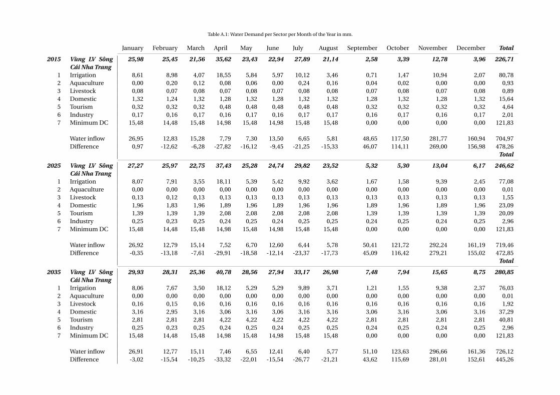
Table A.1: Water Demand per Sector per Month of the Year in mm.
January February March April May June July August September October November December Total
2015 Vùng LV SôngCái Nha Trang
25,98 25,45 21,56 35,62 23,43 22,94 27,89 21,14 2,58 3,39 12,78 3,96 226,71
1 Irrigation 8,61 8,98 4,07 18,55 5,84 5,97 10,12 3,46 0,71 1,47 10,94 2,07 80,782 Aquaculture 0,00 0,20 0,12 0,08 0,06 0,00 0,24 0,16 0,04 0,02 0,00 0,00 0,933 Livestock 0,08 0,07 0,08 0,07 0,08 0,07 0,08 0,08 0,07 0,08 0,07 0,08 0,894 Domestic 1,32 1,24 1,32 1,28 1,32 1,28 1,32 1,32 1,28 1,32 1,28 1,32 15,645 Tourism 0,32 0,32 0,32 0,48 0,48 0,48 0,48 0,48 0,32 0,32 0,32 0,32 4,646 Industry 0,17 0,16 0,17 0,16 0,17 0,16 0,17 0,17 0,16 0,17 0,16 0,17 2,017 Minimum DC 15,48 14,48 15,48 14,98 15,48 14,98 15,48 15,48 0,00 0,00 0,00 0,00 121,83
Water inflow 26,95 12,83 15,28 7,79 7,30 13,50 6,65 5,81 48,65 117,50 281,77 160,94 704,97Difference 0,97 -12,62 -6,28 -27,82 -16,12 -9,45 -21,25 -15,33 46,07 114,11 269,00 156,98 478,26
Total
2025 Vùng LV SôngCái Nha Trang
27,27 25,97 22,75 37,43 25,28 24,74 29,82 23,52 5,32 5,30 13,04 6,17 246,62
1 Irrigation 8,07 7,91 3,55 18,11 5,39 5,42 9,92 3,62 1,67 1,58 9,39 2,45 77,082 Aquaculture 0,00 0,00 0,00 0,00 0,00 0,00 0,00 0,00 0,00 0,00 0,00 0,00 0,013 Livestock 0,13 0,12 0,13 0,13 0,13 0,13 0,13 0,13 0,13 0,13 0,13 0,13 1,554 Domestic 1,96 1,83 1,96 1,89 1,96 1,89 1,96 1,96 1,89 1,96 1,89 1,96 23,095 Tourism 1,39 1,39 1,39 2,08 2,08 2,08 2,08 2,08 1,39 1,39 1,39 1,39 20,096 Industry 0,25 0,23 0,25 0,24 0,25 0,24 0,25 0,25 0,24 0,25 0,24 0,25 2,967 Minimum DC 15,48 14,48 15,48 14,98 15,48 14,98 15,48 15,48 0,00 0,00 0,00 0,00 121,83
Water inflow 26,92 12,79 15,14 7,52 6,70 12,60 6,44 5,78 50,41 121,72 292,24 161,19 719,46Difference -0,35 -13,18 -7,61 -29,91 -18,58 -12,14 -23,37 -17,73 45,09 116,42 279,21 155,02 472,85
Total
2035 Vùng LV SôngCái Nha Trang
29,93 28,31 25,36 40,78 28,56 27,94 33,17 26,98 7,48 7,94 15,65 8,75 280,85
1 Irrigation 8,06 7,67 3,50 18,12 5,29 5,29 9,89 3,71 1,21 1,55 9,38 2,37 76,032 Aquaculture 0,00 0,00 0,00 0,00 0,00 0,00 0,00 0,00 0,00 0,00 0,00 0,00 0,013 Livestock 0,16 0,15 0,16 0,16 0,16 0,16 0,16 0,16 0,16 0,16 0,16 0,16 1,924 Domestic 3,16 2,95 3,16 3,06 3,16 3,06 3,16 3,16 3,06 3,16 3,06 3,16 37,295 Tourism 2,81 2,81 2,81 4,22 4,22 4,22 4,22 4,22 2,81 2,81 2,81 2,81 40,816 Industry 0,25 0,23 0,25 0,24 0,25 0,24 0,25 0,25 0,24 0,25 0,24 0,25 2,967 Minimum DC 15,48 14,48 15,48 14,98 15,48 14,98 15,48 15,48 0,00 0,00 0,00 0,00 121,83
Water inflow 26,91 12,77 15,11 7,46 6,55 12,41 6,40 5,77 51,10 123,63 296,66 161,36 726,12Difference -3,02 -15,54 -10,25 -33,32 -22,01 -15,54 -26,77 -21,21 43,62 115,69 281,01 152,61 445,26
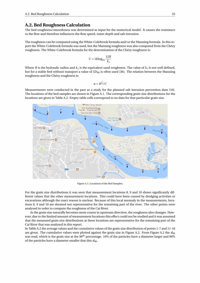
A.2. Bed Roughness Calculation 55
A.2. Bed Roughness CalculationThe bed roughness/smoothness was determined as input for the numerical model. It causes the resistanceto the flow and therefore influences the flow speed, water depth and salt intrusion.
The roughness can be computed using the White-Colebrook formula and/or the Manning formula. In this re-port the White-Colebrook formula was used, but the Manning roughness was also computed from the Chézyroughness. The White-Colebrook formula for the determination of the Chézy roughness is:
C = 18log1012R
ks
Where R is the hydraulic radius and ks is the equivalent sand roughness. The value of ks is not well defined,but for a stable bed without transport a value of 3D90 is often used [36]. The relation between the Manningroughness and the Chézy roughness is:
n = R16 /C
Measurements were conducted in the past as a study for the planned salt intrusion prevention dam [10].The locations of the bed samples are shown in Figure A.1. The corresponding grain size distributions for thelocations are given in Table A.2. Empty table cells correspond to no data for that particular grain size.
Figure A.1: Locations of the Bed Samples.
For the grain size distributions it was seen that measurement locations 8, 9 and 10 shows significantly dif-ferent values that the other measurement locations. This could have been caused by dredging activities orexcavations although the exact reason is unclear. Because of this local anomaly in the measurements, loca-tions 8, 9 and 10 are deemed not representative for the remaining part of the river. The other points wereanalysed in order to compute the roughness of the Cai River.
As the grain size naturally becomes more coarse in upstream direction, the roughness also changes. How-ever, due to the limited amount of measurement locations this effect could not be studied and it was assumedthat the measured grain size distributions at these locations are representative for the remaining part of theCai River that was analysed in this report.In Table A.2 the average values and the cumulative values of the grain size distribution of points 1-7 and 11-16are given. The cumulative values were plotted against the grain size in Figure A.2. From Figure A.2 the d90
was read, which is the grain size at the 90th percentage. 10% of the particles have a diameter larger and 90%of the particles have a diameter smaller that this d90.

A.2. Bed Roughness Calculation 56
Table A.2: Bed Composition at the Different Measurement Locations and the Average and Cumulative Values.
Grain size [mm]
Loc. # <0,005 0,005-1 0,01-0,05 0,05-0,1 0,1-0,25 0,25-0,5 0,5-1 1,0-2,0 2,0-5,0 5,0-10,0 >10
1 0,7 0,2 1,7 5,1 2 8,9 19 27,9 28,1 5,7 0,62 0,2 0,1 0,1 3,7 7,6 21,7 4,8 39,3 18,8 3,63 0,2 0,1 0,1 3,7 7,6 21,7 4,8 39,3 18,8 3,64 4,3 1,9 8,6 14,2 10,6 12,4 20,8 18,1 7,1 1,95 0,2 0,1 0,1 4,8 19,9 29,4 27,8 12,2 5 0,46 0,1 0,1 1,8 3,7 10,7 25,7 33,2 20,5 2,4 1,87 0,4 0,1 0,2 4,4 5,6 15 37,6 30,1 6,1 0,48 37,3 13,5 31,7 9,7 7,6 0,29 34,7 13 30,6 12,5 8,8 0,5
10 31,4 12,2 29,2 13,8 13 0,511 0,2 0,1 0,4 3,8 20,3 65,6 7,8 1,912 0,1 0,2 17,5 29,4 49,7 2,5 0,513 0,4 0,2 0,1 15,4 24 49,4 8,9 1,514 6 4,1 9,7 6,9 1,7 8,9 15,5 26,8 18,1 2,515 3,6 2,1 6,2 10,3 2,4 9,7 19,3 25,4 18,5 2,516 0,2 0,1 0,1 3,9 6,9 16,1 34,6 26,6 9,6 1,8
AVG 1,28 0,70 2,12 7,35 10,90 24,55 17,62 21,75 11,58 1,91 0,18CUM 1,28 1,98 4,10 11,45 22,35 46,90 64,52 86,28 97,86 99,77 99,95
10 2 10 1 100 101
Grain Size [mm]0
10
20
30
40
50
60
70
80
90
100
Siev
e Pe
rcen
tage
Figure A.2: Grading Curve of the Bed Composition in the Cai River.
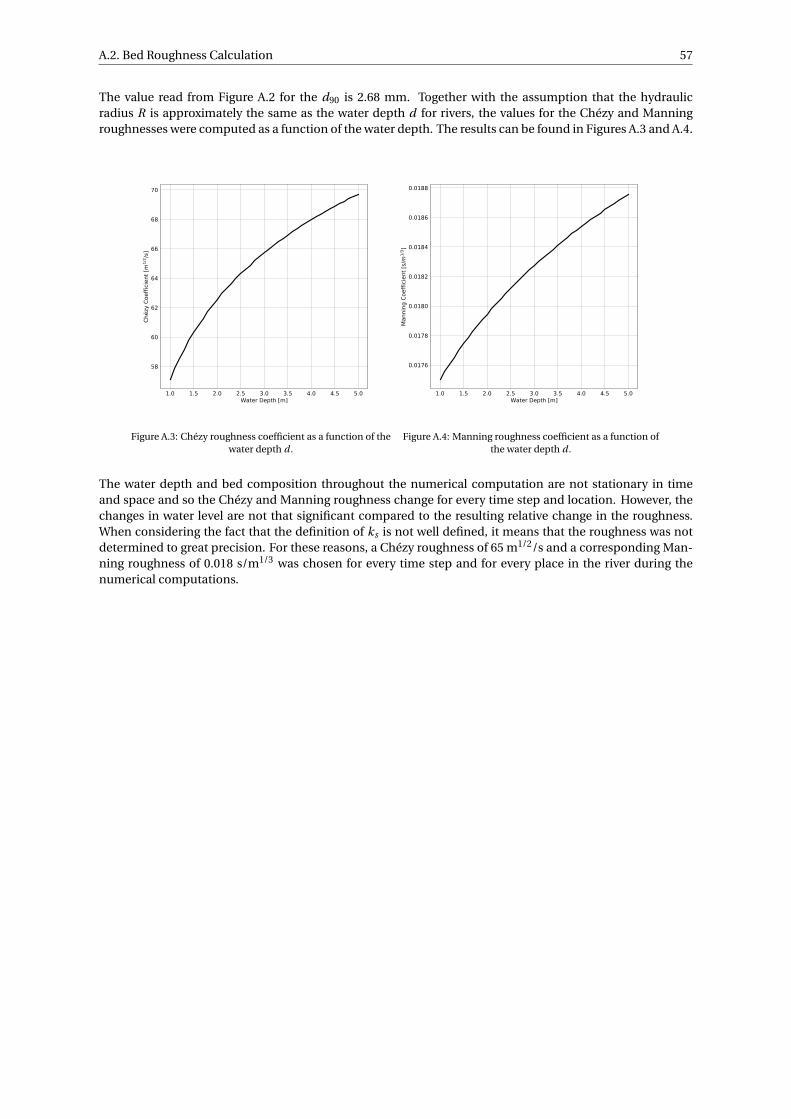
A.2. Bed Roughness Calculation 57
The value read from Figure A.2 for the d90 is 2.68 mm. Together with the assumption that the hydraulicradius R is approximately the same as the water depth d for rivers, the values for the Chézy and Manningroughnesses were computed as a function of the water depth. The results can be found in Figures A.3 and A.4.
1.0 1.5 2.0 2.5 3.0 3.5 4.0 4.5 5.0Water Depth [m]
58
60
62
64
66
68
70
Chéz
y Co
effic
ient
[m1/
2 /s]
Figure A.3: Chézy roughness coefficient as a function of thewater depth d .
1.0 1.5 2.0 2.5 3.0 3.5 4.0 4.5 5.0Water Depth [m]
0.0176
0.0178
0.0180
0.0182
0.0184
0.0186
0.0188
Man
ning
Coe
fficie
nt [s
/m1/
3 ]
Figure A.4: Manning roughness coefficient as a function ofthe water depth d .
The water depth and bed composition throughout the numerical computation are not stationary in timeand space and so the Chézy and Manning roughness change for every time step and location. However, thechanges in water level are not that significant compared to the resulting relative change in the roughness.When considering the fact that the definition of ks is not well defined, it means that the roughness was notdetermined to great precision. For these reasons, a Chézy roughness of 65 m1/2/s and a corresponding Man-ning roughness of 0.018 s/m1/3 was chosen for every time step and for every place in the river during thenumerical computations.
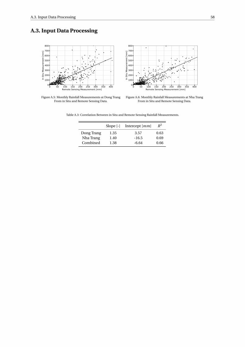
A.3. Input Data Processing 58
A.3. Input Data Processing
0 50 100 150 200 250 300 350 400Remote Sensing Measurement [mm]
0
100
200
300
400
500
600
700
800In
Situ
Mea
sure
men
t [m
m]
Figure A.5: Monthly Rainfall Measurements at Dong TrangFrom in Situ and Remote Sensing Data.
0 50 100 150 200 250 300 350 400Remote Sensing Measurement [mm]
0
100
200
300
400
500
600
700
800
In S
itu M
easu
rem
ent [
mm
]
Figure A.6: Monthly Rainfall Measurements at Nha TrangFrom in Situ and Remote Sensing Data.
Table A.3: Correlation Between in Situ and Remote Sensing Rainfall Measurements.
Slope [-] Intercept [mm] R2
Dong Trang 1.35 3.57 0.63Nha Trang 1.40 -16.5 0.69Combined 1.38 -6.64 0.66
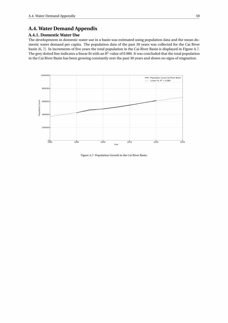
A.4. Water Demand Appendix 59
A.4. Water Demand AppendixA.4.1. Domestic Water UseThe developments in domestic water use in a basin was estimated using population data and the mean do-mestic water demand per capita. The population data of the past 30 years was collected for the Cai Riverbasin [6, 7]. In increments of five years the total population in the Cai River Basin is displayed in Figure A.7.The grey dotted line indicates a linear fit with an R2-value of 0.989. It was concluded that the total populationin the Cai River Basin has been growing constantly over the past 30 years and shows no signs of stagnation.
1980 1990 2000 2010 2020 2030Year
0
200000
400000
600000
800000
1000000
Popu
latio
n Co
unt
Population Count Cai River BasinLinear Fit, R2 = 0.989
Figure A.7: Population Growth in the Cai River Basin.
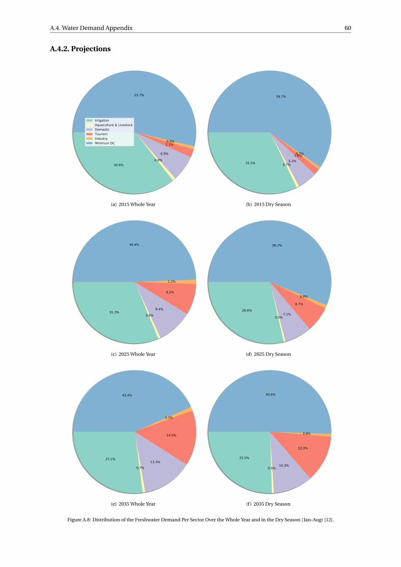
A.4. Water Demand Appendix 60
A.4.2. Projections
35.6%0.8%
6.9%
2.1%0.9%
53.7%
IrrigationAquaculture & LivestockDomesticTourismIndustryMinimum DC
(a) 2015 Whole Year
32.1% 0.7%5.1%
1.6%0.7%
59.7%
(b) 2015 Dry Season
31.3%0.6%
9.4%
8.2%
1.2%
49.4%
(c) 2025 Whole Year
28.6%
0.5%7.1%
6.7%
0.9%
56.2%
(d) 2025 Dry Season
27.1%
0.7%13.3%
14.5%
1.1%
43.4%
(e) 2035 Whole Year
25.5%
0.5%10.3%
12.3%
0.8%
50.6%
(f) 2035 Dry Season
Figure A.8: Distribution of the Freshwater Demand Per Sector Over the Whole Year and in the Dry Season (Jan-Aug) [12].
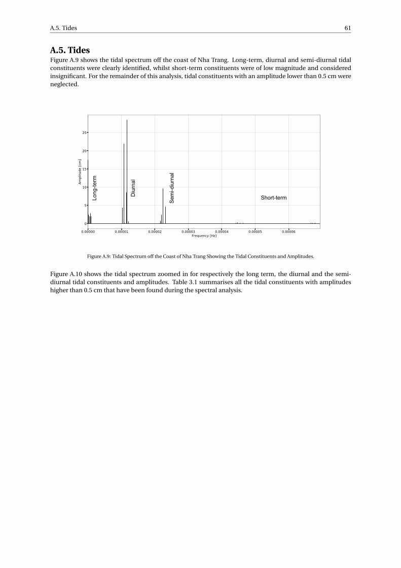
A.5. Tides 61
A.5. TidesFigure A.9 shows the tidal spectrum off the coast of Nha Trang. Long-term, diurnal and semi-diurnal tidalconstituents were clearly identified, whilst short-term constituents were of low magnitude and consideredinsignificant. For the remainder of this analysis, tidal constituents with an amplitude lower than 0.5 cm wereneglected.
Long
-term
Diu
rnal
Sem
i-diu
rnal
Short-term
Figure A.9: Tidal Spectrum off the Coast of Nha Trang Showing the Tidal Constituents and Amplitudes.
Figure A.10 shows the tidal spectrum zoomed in for respectively the long term, the diurnal and the semi-diurnal tidal constituents and amplitudes. Table 3.1 summarises all the tidal constituents with amplitudeshigher than 0.5 cm that have been found during the spectral analysis.
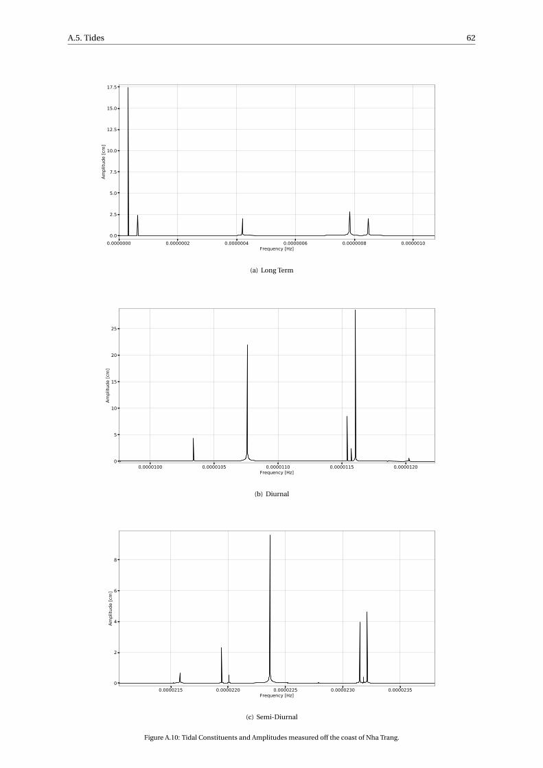
A.5. Tides 62
0.0000000 0.0000002 0.0000004 0.0000006 0.0000008 0.0000010Frequency [Hz]
0.0
2.5
5.0
7.5
10.0
12.5
15.0
17.5
Ampl
itude
[cm
]
(a) Long Term
0.0000100 0.0000105 0.0000110 0.0000115 0.0000120Frequency [Hz]
0
5
10
15
20
25
Ampl
itude
[cm
]
(b) Diurnal
0.0000215 0.0000220 0.0000225 0.0000230 0.0000235Frequency [Hz]
0
2
4
6
8
Ampl
itude
[cm
]
(c) Semi-Diurnal
Figure A.10: Tidal Constituents and Amplitudes measured off the coast of Nha Trang.

A.6. Estuarine Richardson Number 63
A.6. Estuarine Richardson NumberThe estuarine Richardson number is calculated according the following formula:
NR = ∆ρ
ρ f
g h
ν2
Q f T
E A0(A.1)
where:
• ∆ρ = ρ−ρ f
• ρ = 1021 kg/m3 is the saltwater density
• ρ f = 1000 kg/m3 is the freshwater density
• g = 9.8 m/s2 is the gravitational acceleration
• h = 3.81 m is the mean water depth
• ν=πE/T [m/s] is the tidal velocity amplitude
• E = 16000 m is the tidal excursion length
• T = 86400 s is the tidal period
• Q f = 10 m3/s is the river discharge
• A0 = B0h [m2] is the effective cross-sectional area of the river mouth
• B0 = 370 m is the effective width of the river mouth

A.7. Delft3D Input 64
A.7. Delft3D InputMany input parameters are required to model the estuary in Delft3D. Table A.4 gives an overview of all theinput parameters of the model.
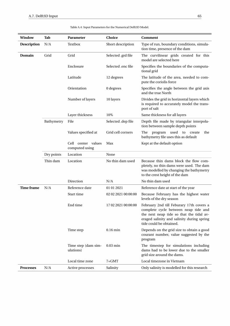
A.7. Delft3D Input 65
Table A.4: Input Parameters for the Numerical Delft3D Model.
Window Tab Parameter Choice Comment
Description N/A Textbox Short description Type of run, boundary conditions, simula-tion time, presence of the dam
Domain Grid Grid Selected .grd file The curvilinear grids created for thismodel are selected here
Enclosure Selected .enc file Specifies the boundaries of the computa-tional grid
Latitude 12 degrees The latitude of the area, needed to com-pute the coriolis force
Orientation 0 degrees Specifies the angle between the grid axisand the true North
Number of layers 10 layers Divides the grid in horizontal layers whichis required to accurately model the trans-port of salt
Layer thickness 10% Same thickness for all layers
Bathymetry File Selected .dep file Depth file made by triangular interpola-tion between sample depth points
Values specified at Grid cell corners The program used to create thebathymetry file uses this as default
Cell center valuescomputed using
Max Kept at the default option
Dry points Location None
Thin dam Location No thin dam used Because thin dams block the flow com-pletely, no thin dams were used. The damwas modelled by changing the bathymetryto the crest height of the dam
Direction N/A No thin dam used
Time frame N/A Reference date 01 01 2021 Reference date at start of the year
Start time 02 02 2021 00:00:00 Because February has the highest waterlevels of the dry season
End time 17 02 2021 00:00:00 February 2nd till Feburary 17th covers acomplete cycle between neap tide andthe next neap tide so that the tidal av-eraged salinity and salinity during springtide could be obtained.
Time step 0.16 min Depends on the grid size to obtain a goodcourant number, value suggested by theprogram
Time step (dam sim-ulations)
0.03 min The timestep for simulations includingdams had to be lower due to the smallergrid size around the dams.
Local time zone 7+GMT Local timezone in Vietnam
Processes N/A Active processes Salinity Only salinity is modelled for this research
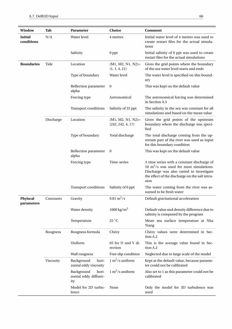
A.7. Delft3D Input 66
Window Tab Parameter Choice Comment
Initialconditions
N/A Water level 4 metres Initial water level of 4 metres was used tocreate restart files for the actual simula-tions
Salinity 0 ppt Initial salinity of 0 ppt was used to createrestart files for the actual simulations
Boundaries Tide Location (M1, M2, N1, N2)=(1, 1, 4, 21)
Gives the grid points where the boundaryof the sea water level starts and ends
Type of boundary Water level The water level is specified on this bound-ary
Reflection parameteralpha
0 This was kept on the default value
Forcing type Astronomical The astronomical forcing was determinedin Section A.5
Transport conditions Salinity of 33 ppt The salinity in the sea was constant for allsimulations and based on the mean value
Discharge Location (M1, M2, N1, N2)=(242, 242, 4, 17)
Gives the grid points of the upstreamboundary where the discharge was speci-fied
Type of boundary Total discharge The total discharge coming from the up-stream part of the river was used as inputfor this boundary condition
Reflection parameteralpha
0 This was kept on the default value
Forcing type Time-series A time series with a constant discharge of10 m3/s was used for most simulations.Discharge was also varied to investigatethe effect of the discharge on the salt intru-sion
Transport conditions Salinity of 0 ppt The water coming from the river was as-sumed to be fresh water
Phyiscalparameters
Constants Gravity 9.81 m2/s Default gravitational acceleration
Water density 1000 kg/m3 Default value and density difference due tosalinity is computed by the program
Temperature 25 ◦C Mean sea surface temperature at NhaTrang
Rougness Rougness formula Chézy Chézy values were determined in Sec-tion A.2
Uniform 65 for U and V di-rection
This is the average value found in Sec-tion A.2
Wall rougness Free slip condition Neglected due to large scale of the model
Viscosity Background hori-zontal eddy viscosity
1 m2/s uniform Kept at the default value, because parame-ter could not be calibrated
Background hori-zontal eddy diffusiv-ity
1 m2/s uniform Also set to 1 as this parameter could not becalibrated
Model for 2D turbu-lence
None Only the model for 3D turbulence wasused
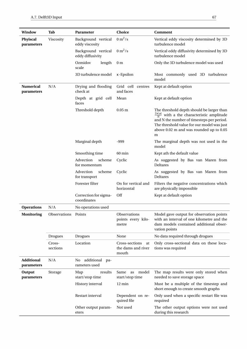
A.7. Delft3D Input 67
Window Tab Parameter Choice Comment
Phyiscalparameters
Viscosity Background verticaleddy viscosity
0 m2/s Vertical eddy viscosity determined by 3Dturbulence model
Background verticaleddy diffusivity
0 m2/s Vertical eddy diffusivity determined by 3Dturbulence model
Ozmidov lengthscale
0 m Only the 3D turbulence model was used
3D turbulence model κ-Epsilon Most commonly used 3D turbulencemodel
Numericalparameters
N/A Drying and floodingcheck at
Grid cell centresand faces
Kept at default option
Depth at grid cellfaces
Mean Kept at default option
Threshold depth 0.05 m The threshold depth should be larger than2π|a|
N with a the characteristic amplitudeand N the number of timesteps per period.The threshold value for our model was justabove 0.02 m and was rounded up to 0.05m
Marginal depth -999 The marginal depth was not used in themodel
Smoothing time 60 min Kept ath the default value
Advection schemefor momentum
Cyclic As suggested by Bas van Maren fromDeltares
Advection schemefor transport
Cyclic As suggested by Bas van Maren fromDeltares
Forester filter On for vertical andhorizontal
Filters the negative concentrations whichare physically impossible
Correction for sigma-coordinates
Off Kept at default option
Operations N/A No operations used
Monitoring Observations Points Observationspoints every kilo-metre
Model gave output for observation pointswith an interval of one kilometre and thedam models contained additional obser-vation points
Drogues Drogues None No data required through drogues
Cross-sections
Location Cross-sections atthe dams and rivermouth
Only cross-sectional data on these loca-tions was required
Additionalparameters
N/A No additional pa-rameters used
Outputparameters
Storage Map resultsstart/stop time
Same as modelstart/stop time
The map results were only stored whenneeded to save storage space
History interval 12 min Must be a multiple of the timestep andshort enough to create smooth graphs
Restart interval Dependent on re-quired file
Only used when a specific restart file wasrequired
Other output param-eters
Not used The other output options were not usedduring this research
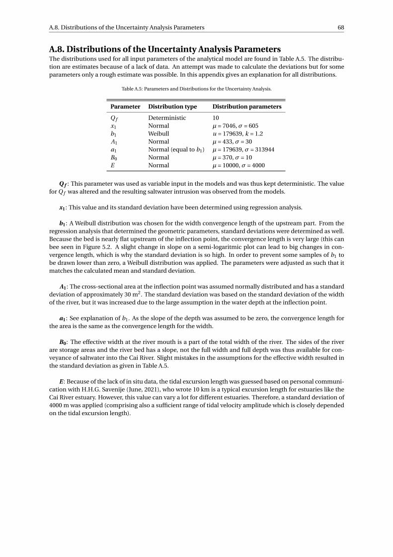
A.8. Distributions of the Uncertainty Analysis Parameters 68
A.8. Distributions of the Uncertainty Analysis ParametersThe distributions used for all input parameters of the analytical model are found in Table A.5. The distribu-tion are estimates because of a lack of data. An attempt was made to calculate the deviations but for someparameters only a rough estimate was possible. In this appendix gives an explanation for all distributions.
Table A.5: Parameters and Distributions for the Uncertainty Analysis.
Parameter Distribution type Distribution parameters
Q f Deterministic 10x1 Normal µ = 7046, σ = 605b1 Weibull u = 179639, k = 1.2A1 Normal µ = 433, σ = 30a1 Normal (equal to b1) µ = 179639, σ = 313944B0 Normal µ = 370, σ = 10E Normal µ = 10000, σ = 4000
Q f : This parameter was used as variable input in the models and was thus kept deterministic. The valuefor Q f was altered and the resulting saltwater intrusion was observed from the models.
x1: This value and its standard deviation have been determined using regression analysis.
b1: A Weibull distribution was chosen for the width convergence length of the upstream part. From theregression analysis that determined the geometric parameters, standard deviations were determined as well.Because the bed is nearly flat upstream of the inflection point, the convergence length is very large (this canbee seen in Figure 5.2. A slight change in slope on a semi-logaritmic plot can lead to big changes in con-vergence length, which is why the standard deviation is so high. In order to prevent some samples of b1 tobe drawn lower than zero, a Weibull distribution was applied. The parameters were adjusted as such that itmatches the calculated mean and standard deviation.
A1: The cross-sectional area at the inflection point was assumed normally distributed and has a standarddeviation of approximately 30 m2. The standard deviation was based on the standard deviation of the widthof the river, but it was increased due to the large assumption in the water depth at the inflection point.
a1: See explanation of b1. As the slope of the depth was assumed to be zero, the convergence length forthe area is the same as the convergence length for the width.
B0: The effective width at the river mouth is a part of the total width of the river. The sides of the riverare storage areas and the river bed has a slope, not the full width and full depth was thus available for con-veyance of saltwater into the Cai River. Slight mistakes in the assumptions for the effective width resulted inthe standard deviation as given in Table A.5.
E : Because of the lack of in situ data, the tidal excursion length was guessed based on personal communi-cation with H.H.G. Savenije (June, 2021), who wrote 10 km is a typical excursion length for estuaries like theCai River estuary. However, this value can vary a lot for different estuaries. Therefore, a standard deviation of4000 m was applied (comprising also a sufficient range of tidal velocity amplitude which is closely dependedon the tidal excursion length).


![CHAPTER 8 Effects of land-use changes and groundwater ... · lowering of water table by drainage canals also leads to saltwater intrusion [1]. Generally, the shape and extent of saltwater-intruded](https://img.pdfslide.us/doc/110x75/5edd2ca8ad6a402d66682aaf/chapter-8-effects-of-land-use-changes-and-groundwater-lowering-of-water-table.jpg)