Louisiana State UniversityLSU Digital Commons

LSU Master's Theses Graduate School

2004

Assessment of shearing phenomenon and porosityof porous media using microfocus computedtomographyBashar Adeeb AlramahiLouisiana State University and Agricultural and Mechanical College, balram1@lsu.edu

Follow this and additional works at: https://digitalcommons.lsu.edu/gradschool_theses

Part of the Civil and Environmental Engineering Commons

This Thesis is brought to you for free and open access by the Graduate School at LSU Digital Commons. It has been accepted for inclusion in LSUMaster's Theses by an authorized graduate school editor of LSU Digital Commons. For more information, please contact gradetd@lsu.edu.

Recommended CitationAlramahi, Bashar Adeeb, "Assessment of shearing phenomenon and porosity of porous media using microfocus computedtomography" (2004). LSU Master's Theses. 1337.https://digitalcommons.lsu.edu/gradschool_theses/1337

ASSESSMENT OF SHEARING PHENOMENON AND POROSITY OF POROUS MEDIA USING MICROFOCUS COMPUTED

TOMOGRAPHY

A Thesis

Submitted to the Graduate School of the Louisiana State University and

Agricultural and Mechanical College in partial fulfillment of the

requirements for the degree of Master of Science in Civil Engineering

in

The Department of Civil and Environmental Engineering

By Bashar A. Alramahi

B.Sc. Birzeit University, Ramallah, Palestine 2002 August, 2004

ii

DEDICATION

To the memory of my father

To my mother and brother

&

To my family and friends

iii

ACKNOWLEDGMENTS

First, I would like to express my deepest thanks to my family. I am really grateful

for all the love and support they always provided.

I would like to acknowledge the efforts of my advisor Dr. Khalid Alshibli. The

help and guidance he provided for me throughout my graduate study at Louisiana State

University are deeply appreciated. I would like to extend my thanks to the members of

my committee, Dr. Dante Fratta and Dr. Emir Macari. I am grateful of all the help and

support they always provided.

I would like to thank my dear friends, Dr. Mustafa Alsaleh, Sacit, Victor, Lynne,

Heath, Rich, Brenda and Munir for all the great times we spent together. I would also like

to acknowledge the contribution of Patrik Furlong, Irshad Syed and Vida Sharafkhani

from Louisiana State University for help in the data collection.

Special thanks are due to Dr. Ron Beshears and Mr. David Myers of NASA/

Marshall Space Flight center for helping us to perform the CT scans of the plastic beads.

I thank Professor Balasingam Muhunthan, director of WAX-CT Laboratory and

Mohammad Reza Razavi, Graduate student of Washington State University for allowing

us to perform the CT scans of the rock cores, I also thank Mr. David Philips of HYTEC

Inc. for providing the FlashCT_VIZ software.

This research is partially funded by the Louisiana Transportation Research Center

(LTRC Project No. 02-07GT) and the Louisiana Department of Transportation and

Development (State Project No. 736-99-1057) through Transportation Innovation for

Research Exploration (TIRE) program.

iv

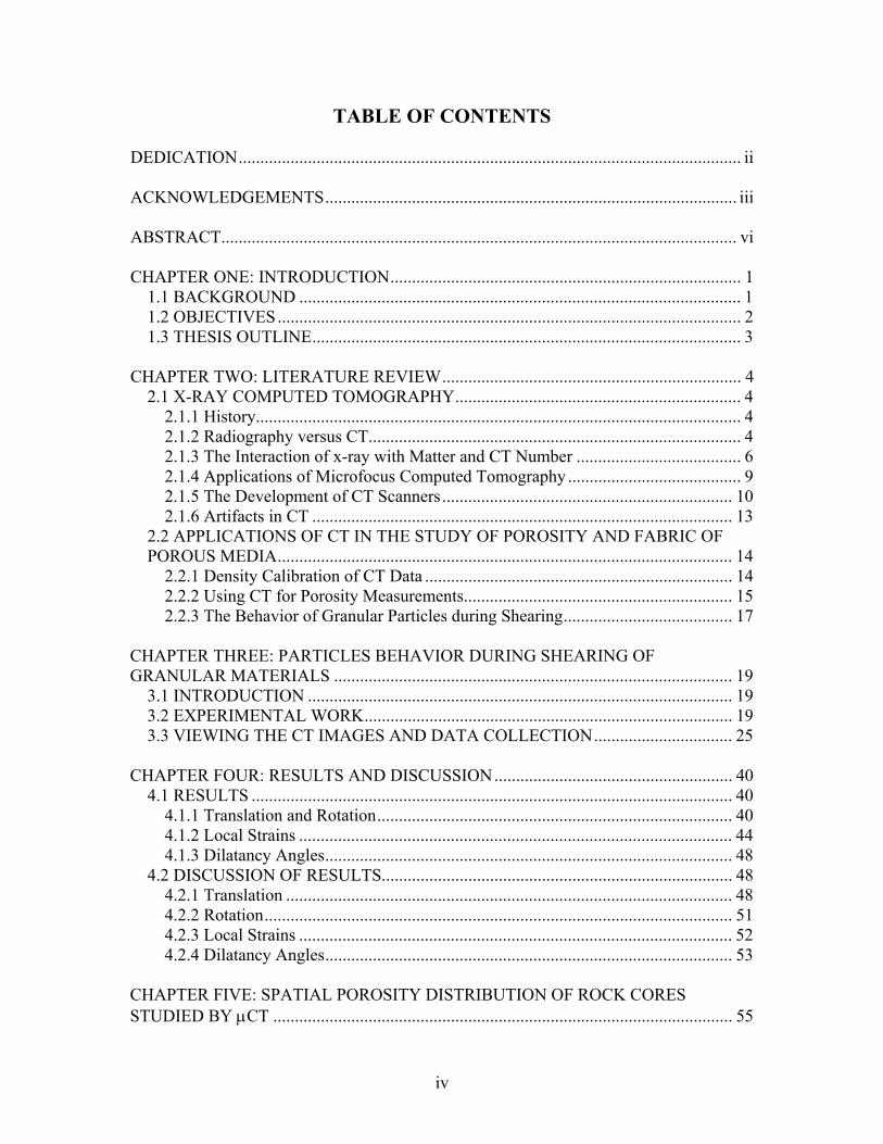
TABLE OF CONTENTS DEDICATION.................................................................................................................... ii ACKNOWLEDGEMENTS............................................................................................... iii ABSTRACT....................................................................................................................... vi CHAPTER ONE: INTRODUCTION................................................................................. 1

1.1 BACKGROUND ...................................................................................................... 1 1.2 OBJECTIVES........................................................................................................... 2 1.3 THESIS OUTLINE................................................................................................... 3

CHAPTER TWO: LITERATURE REVIEW..................................................................... 4

2.1 X-RAY COMPUTED TOMOGRAPHY.................................................................. 4 2.1.1 History................................................................................................................ 4 2.1.2 Radiography versus CT...................................................................................... 4 2.1.3 The Interaction of x-ray with Matter and CT Number ...................................... 6 2.1.4 Applications of Microfocus Computed Tomography ........................................ 9 2.1.5 The Development of CT Scanners................................................................... 10 2.1.6 Artifacts in CT ................................................................................................. 13

2.2 APPLICATIONS OF CT IN THE STUDY OF POROSITY AND FABRIC OF POROUS MEDIA......................................................................................................... 14

2.2.1 Density Calibration of CT Data ....................................................................... 14 2.2.2 Using CT for Porosity Measurements.............................................................. 15 2.2.3 The Behavior of Granular Particles during Shearing....................................... 17

CHAPTER THREE: PARTICLES BEHAVIOR DURING SHEARING OF GRANULAR MATERIALS ............................................................................................ 19

3.1 INTRODUCTION .................................................................................................. 19 3.2 EXPERIMENTAL WORK..................................................................................... 19 3.3 VIEWING THE CT IMAGES AND DATA COLLECTION................................ 25

CHAPTER FOUR: RESULTS AND DISCUSSION....................................................... 40

4.1 RESULTS ............................................................................................................... 40 4.1.1 Translation and Rotation.................................................................................. 40 4.1.2 Local Strains .................................................................................................... 44 4.1.3 Dilatancy Angles.............................................................................................. 48

4.2 DISCUSSION OF RESULTS................................................................................. 48 4.2.1 Translation ....................................................................................................... 48 4.2.2 Rotation............................................................................................................ 51 4.2.3 Local Strains .................................................................................................... 52 4.2.4 Dilatancy Angles.............................................................................................. 53

CHAPTER FIVE: SPATIAL POROSITY DISTRIBUTION OF ROCK CORES STUDIED BY µCT .......................................................................................................... 55

v

5.1 INTRODUCTION .................................................................................................. 55 5.2 EXPERIMENTAL WORK..................................................................................... 55

5.2.1 Specimen Description ...................................................................................... 55 5.2.2 CT Scanning..................................................................................................... 57

5.3 POROSITY CALCULATIONS ............................................................................. 59 5.3.1 Density Calibration .......................................................................................... 59

5.4 RESULTS AND DISCUSSION............................................................................. 61 5.4.1 Effect of Grain Size Distribution ..................................................................... 61 5.4.2 Effect of Compaction Pressure ........................................................................ 64 5.4.3 Vertical Profiles of Porosity............................................................................. 68

CHAPTER SIX: CONCLUSIONS AND RECOMMENDATIONS ............................... 70

6.1 CONCLUSIONS..................................................................................................... 70 6.2 RECOMMENDATIONS........................................................................................ 72

REFERENCES ................................................................................................................. 73

APPENDIX A: TRANSLATION AND ROTATION HISTOGRAMS........................... 76

APPENDIX B: LOCAL STRAIN HISTOGRAMS ......................................................... 78

VITA................................................................................................................................. 82

vi

ABSTRACT

Microfocus x-ray computed tomography (µCT) is a powerful non-destructive

scanning technique to study the internal fabric of granular materials. In this thesis, µCT

was applied to two cases. The first case involves studying the behavior of particles in a

triaxial specimen during shearing. Three-dimensional translation and rotation of the

particles were tracked throughout the shearing process, and they were used to calculate

the local strain distributions including the axial, radial, and rotation strains. Moreover, the

local dilatancy angle distribution was calculated for all the different levels of the

experiment. These distributions were compared to study the changes in the behavior of

the particles at different stages of the test. Furthermore, 3D renderings and animations

showing the particles behavior throughout the test were generated.

It was noticed that the radial strains εx and εy showed a similarity throughout the test

due to the axisymmetric conditions of the test. It was also found that high rotation angles

took place, where the vertical rotation component reached up to 30 degrees and the

horizontal rotation reached up to 60 degrees. Furthermore, the rotation strain component

reached up to about 50% at the end of the test. On the other hand, a wide range of local

dilatancy angles was observed, where the values varied between -50 degrees and 70

degrees, and the fraction of the positive values (dilation) increased as the test proceeds.

The second part of this thesis aims at determining the effect of grain size

distribution and consolidation pressure on the spatial porosity distribution of synthetic

rock cores. Twelve rock cores were prepared with different grain size distributions and

consolidation pressures, and scanned using a high resolution µCT system. Density

calibration was conducted to correlate the CT numbers to the bulk density, and the

vii

porosity of the cores. A computer algorithm was developed to calculate the local porosity

values, producing about 15 million values per core. µCT showed an excellent ability to

track the changes in the local porosity distribution of the cores. It was found that grain

size distribution has a larger effect on the porosity values, where a noticeable decrease in

the porosity values was observed when using well graded grains. On the other hand,

increasing the consolidation pressure did not always decrease the porosity values. This

could be due to the crushing of the particles at very high consolidation pressures.

CHAPTER ONE

INTRODUCTION

1.1 BACKGROUND

To study the mechanical behavior of granular materials, many factors should be

considered, like the particles’ arrangement, particle groups’ association, packing density, particle

shapes, and the inter-particle configuration. The analysis techniques for these factors are usually

classified as destructive and non destructive. Destructive techniques include specimen

stabilization and thin sectioning, while the nondestructive techniques include magnetic resonance

imaging, ultrasonic testing, x-ray radiography and x-ray computed tomography (Alshibli et al.,

2000a).

Computed tomography is an imaging technique in which an object is placed between an

x-ray source and a detector, and the object is rotated while the x-ray passes through it collecting

information about its internal structure. The information is reconstructed to create a two-

dimensional cross section “slice” of the object that can be used to view the internal structure of

the object (Cromwell, 1984). Slices can also be stacked together to create a three dimensional

volume view of the scanned object. Alshibli et. al (2000a) showed that CT is able to detect

specimens’ inhomogeneities, localization patterns, and quantify void ratio variation within sand

specimens.

Many numerical and experimental efforts have been made to understand and predict the

behavior of granular materials during shearing. Many assumptions had been made to describe the

sliding and rolling of the particles during shearing. The non-destructive visualization abilities

provided by CT makes it possible to achieve a better understanding of the particles’ interaction

during shearing at the microscopic level. This will help to improve the modeling of the

1

constitutive behavior of granular materials. It also could be used to validate the previous

assumptions about the particles’ behavior.

Investigating the spatial distribution of porosity in rock cores is of great importance in

petroleum engineering and ground water hydrology. Recent advances in computed tomography

have increased the potential of conducting an accurate assessment of porosity distribution within

rock cores and linking such measurements to other physical properties such as permeability and

pore space distribution. CT is a very effective tool to study this property. It has the ability to

detect the effects of small change in particle size distribution and compaction pressure of rock

cores on their porosity distribution. The results of this research might result in improving current

models that link porosity of rocks to their permeability and tortuosity..

1.2 OBJECTIVES

The main objective of this thesis is to apply microfocus computed tomography to study

micro-properties of geomaterials. Two cases will be studied; they are:

I) Study the shearing of granular materials: a triaxial specimen was scanned at different

strain levels to track the translation and rotation of the particles within the specimen. The

obtained values for translation and rotation will be used to calculate the local strain

distribution within the specimen. And the distributions will be compared to study the

behavior of the particles at different stages of the experiment. Also, three dimensional

renderings and animations will be generated in order to show the particle movement and

rotation throughout the experiment.

II) Characterize the variation of the local porosity of rock cores: assess spatial porosity

distribution of synthetic rock cores, and the effect of using different compaction pressures

and different grain size distributions on these values.

2

1.3 THESIS OUTLINE

Chapter 2 of this thesis will present a literature review about x-ray computed

tomography, including a description of the scanning process, the engineering applications, the

development of CT scanners, and artifacts in CT images. It also presents some of the previous

efforts in the field of studying the behavior of granular materials during shearing and porosity

measurements.

A description of the experimental work conducted in order to achieve the first objective,

including the materials used, specimen preparation and the scanning process is presented in

Chapter 3. It also includes the methods used to view the CT images and data collection. Chapter

4 includes a presentation of the results of this study, along with the analysis and discussion of

these results.

The experimental work conducted in order to achieve the second objective, a description

of the rock cores and the CT scanning process, and the results of the study are presented in

Chapter 5. The conclusion of this thesis along with the remarks and recommendations for future

work are presented in Chapter 6.

3

CHAPTER TWO

LITERATURE REVIEW

2.1 X-RAY COMPUTED TOMOGRAPHY

2.1.1 History

X-ray was originally discovered by the German physicist Wilhelm Konrad Rontgen in

1895, for that he was awarded the Nobel Prize in physics in 1901. Since then, X-ray radiography

was widely used in the medical field to view and diagnose internal body organs (KTH, 2001).

Applications of radiography extended from the medical field to industrial applications as

a very useful non destructive tool to investigate the internal structure of the bodies. But the

capabilities of radiography were limited to providing a 2D projection of the internal structure of

a body, which could not provide enough details (Sheats, 2000).

In 1971 Godfrey Hounsfield of England’s EMI laboratories developed the technology

known as Computed tomography, in which detailed internal structural information about the

body could be obtained (Barrington, 2004).

2.1.2 Radiography versus CT

A neutron or x-ray source and a piece of film are used in radiography. When the radiation

passes through an object it is attenuated, and a projection of the internal structure is created when

the x-ray reaches the film (Sheats, 2000). Therefore, the three dimensional (3D) structure of the

body is represented by a 2D projection, and the depth dimensions are lost where all the planes

perpendicular to the direction of the x-ray are superimposed over each other.

4

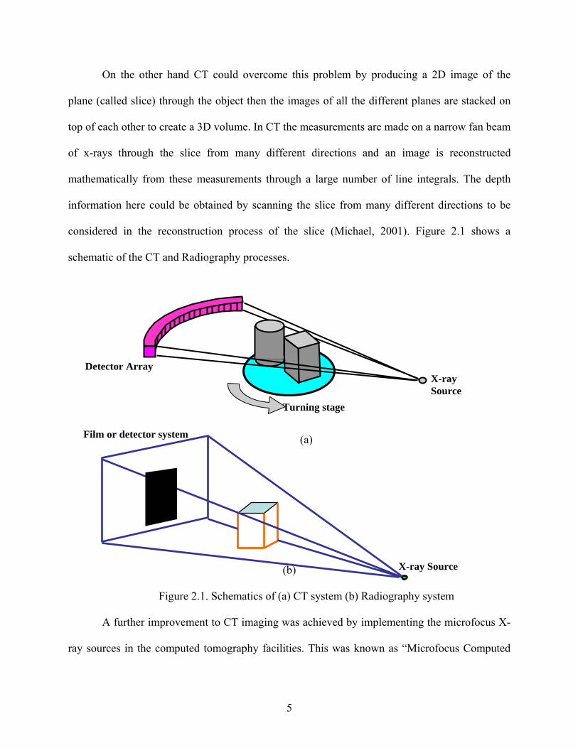
On the other hand CT could overcome this problem by producing a 2D image of the

plane (called slice) through the object then the images of all the different planes are stacked on

top of each other to create a 3D volume. In CT the measurements are made on a narrow fan beam

of x-rays through the slice from many different directions and an image is reconstructed

mathematically from these measurements through a large number of line integrals. The depth

information here could be obtained by scanning the slice from many different directions to be

considered in the reconstruction process of the slice (Michael, 2001). Figure 2.1 shows a

schematic of the CT and Radiography processes.

Detector Array

X-ray Source

Turning stage Film or detector system (a)

X-ray Source (b)

Figure 2.1. Schematics of (a) CT system (b) Radiography system

A further improvement to CT imaging was achieved by implementing the microfocus X-

ray sources in the computed tomography facilities. This was known as “Microfocus Computed

5

Tomography µCT”. This technology uses a new type of X-ray tube whose X-ray focus is from a

fraction of a micron to 10 µm. It mainly has an acceleration voltage from 100 kV to 225 kV.

Using this tube largely magnified the projection data of the object without degradation of the

sharpness obtained (Fujii, 2003). Using µCT enhanced the resolution of the systems to the order

of ( 10µm x 10 µm x 10 µm) for small objects instead of (60 µm x 60 µm x 1 mm) obtained by

the conventional CT systems (Wevers et al., 2000). Moreover, it can be realized that using µCT,

the same high resolution could be obtained in the z-direction, reducing the thickness of the slice,

and improving the CT image quality.

2.1.3 The Interaction of x-ray with Matter and CT Number

When the x-ray passes through matter, the photons are either scattered with some loss of

energy, or completely absorbed in a photoelectric interaction, as a result, some photons will be

lost from the beam while passing through matter. Only part of the photons will remain in the

beam and reach to the detector, which means that a beam of photons is not degraded in energy as

a result of passing through matter, just attenuated in intensity (KTH, 2001).

The probability of photon attenuation can be expressed per thickness of the attenuator, with the

Beer equation:

I(x) = I0 e-µx.…………………………………………………. ………. (2.1)

Where I is the x-ray intensity at certain distance x, I0 is the x-ray intensity when it is emitted

from the source, and µ is the linear attenuation coefficient which can be defined as the

probability that an x-ray or gamma-ray photon will interact with the material it is traversing per

unit path length traveled. It is usually reported in cm-1. The linear attenuation coefficient depends

on the photon energy, the chemical composition and physical density of the material (Amersham

Health, 2003). Usually, the dependency of the linear attenuation on the density of the material is

6

overcome by normalizing it to the density. The normalized value of the linear attenuation is

called the mass attenuation (µ/ρ). The mass attenuation for any material can be calculated as the

weighted average of the mass attenuations of the component elements, where the mass

attenuation of each element is multiplied by its fracture by weight of the composite (Amersham

Health, 2003).

The obtained CT numbers in a CT scan are directly proportional to the local electron

density of the material under investigation (Bossi el al. 1990). The CT scanner measures density

as a CT number (Alfaro et al. 2001), which is defined as (Otani et al. 2000):

w

wtCTNµ

κµµ )( −= ………………………………… (2.2)

Where µt is the linear attenuation of the material and µw is the linear attenuation of water, and k

is a scaling factor either 500 or 1000 (Alfaro, 2001). However, different CT scanners generate

different CT number ranges (k) depending on their reconstruction algorithms.

If a pixel (or a voxel which is a three dimensional pixel) lies in more than one material

the CT number for this pixel is calculated as the weighted average of the CT numbers of the

different materials considering the percentage of the volume occupied by the material from the

total voxel volume.

The standard mass attenuation coefficients (µ/ρ) can be obtained for different materials

from The National Institute of Standards and Technology (NIST) website, and the mass

attenuation of composite materials can always be calculated as the sum of the mass attenuation

of each material in the mixture multiplied by its fraction weight (wi). i.e;

…………………………………………… (2.3) ii

iw )/(/ ρµρµ ∑=

7

This also applies to dry or saturated soil samples where the mass attenuation is calculated

considering the mass attenuations of the soil and water (or air) and their fraction by weight.

Depending on the value of the CT number, pixels take different color intensities between

black and white (gray scale). This scale is set in 256 grey levels, starting from black for low CT

values and ending in white for high CT values. In other words, light materials (like air) appear in

the CT image as black or dark grey pixels, and denser materials (like soil minerals) have a lighter

color, getting closer to the white color as density increases. A sample slice image obtained by CT

is shown in Figure 2.2. Stacking slices together results in creating a volumetric view of the

scanned object. A sample volume view is shown in Figure 2.3.

Figure 2.2. A sample CT slice (Alshibli, 2004)

8

Figure 2.3. Visualization of the volume (Alshibli, 2004)

2.1.4 Applications of Microfocus Computed Tomography

µCT was first used in diagnostic medical fields to acquire 3D images of the internal body

organs and tissues. First it was used to scan the human head, and then it was used all over the

body. In the field of materials research, it was widely used in petroleum engineering for core

analysis, µCT images were used for characterization of reservoir rocks, for mineral formation

and rock property evaluation (e.g. Honarpour et al. 1985). It was also used for monitoring two

and three-phase experiments in porous media (e.g. Bansal et al. 1991) and to verify and analyze

the multiphase fluid flow in porous media (e.g. Cromwell et al. 1984). In the field of

geotechnical engineering, µCT was used to observe localized deformations and shear bands in

specimens undergoing triaxial compression, void ratio evolution inside shear bands, void ratio

variation in soil specimens, and characterization of failure in soils. (Desrues et al. 1996, Otani et

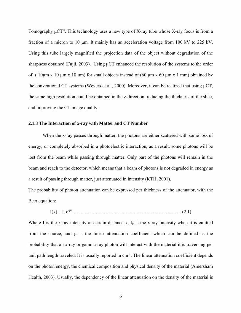
al. 2000, Alshibli et al. 2000a,b). Figure 2.4 shows an example of using µCT images to view the

deformation of a specimen undergoing a triaxial compression test.

9

Figure 2.4. The deformation of a specimen in a triaxial test (Alshibli, 2004)

2.1.5 The Development of CT Scanners

The majority of the CT scanners in use are classified to five generations, which mainly

differ in mechanical configuration of the equipment, the relative motion of the scanned object,

the x-ray source, the detectors, and the amount of the x-ray energy (Figure 2.5). The type of the

scanner will influence the CT image quality, and scanning times, therefore, a tradeoff between

the scanning time and quality (resolution) of the images must take place. For example in the

medical field the patient is required to remain motionless until the scanning process is finished,

therefore, time is a very important factor in medical CT. Moreover, the amount of energy to be

used must be low to be tolerated by the human body. On the other hand, in industrial CT time is

a less important factor and better quality images could be obtained utilizing the availability of a

greater scanning time. Higher energies could be used without affecting the scanned object.

(Kropas-Hughes et al. 2000)

First generation CT scanners use a single x-ray source and a single detector, this

geometry is called: Parallel Beam Geometry. Multiple measurements of the x-ray transmission

are obtained using a single highly collimated x-ray pencil beam and detector (Yoshikawa, 2004).

The x-ray source and detector are translated along the scanned object to obtain a single view, and

10

then they are rotated to obtain another view. Then all the views are collected to build a slice. This

is called a “Translation-Rotation” motion which yields good quality images but it needs a very

long time to perform.

Second generation CT scanners use the same “Translation-Rotation” motion but instead

of having a single x-ray beams, a fan beam of radiation and a linear array of detectors are used.

This enables the scanner to obtain multiple views of the object within a single translation,

resulting in reducing the scanning time by about 10 times for each slice ( Kropas-Hughes et al.

2000).

In third generation CT scanner, a curved detector array containing a large number of

detectors is used with the x-ray source to obtain a complete view of the object without

translation. Multiple views are obtained by the rotation of the source and the detector arrays

around the object. This is called a “Rotate only” motion, and it reduces the scanning time to a

small fraction of the time needed by the first two generations. In this type of scanners, the quality

(resolution) of the obtained images, depend mainly on the number and size of the sensors in the

detector. Therefore, a very large number of sensors has to be used in order to get an acceptable

quality for the images, but it is still hard to get the same quality for the image as in the first and

second generation systems (Kropas-Hughes et al. 2000).

Fourth generation CT scanners also use the “Rotate only” motion, but it is different from

the third generation since it uses a stationary circular array of detectors. The source rotates

around the body shooting a wide fan beam of x-ray. A view is made by obtaining successive

absorption measurements of a single detector at successive positions of the x-ray source. These

scanners are faster and have a better artifacts resistance than the other CT scanners, but they are

more susceptible to scattered radiation (Yoshikawa, 2004).

11

Fifth generation CT scanners are different than all the other scanners since no motion is

involved. In this scanner, a circular array of x-ray sources, which are electronically turned on and

off is used. The detectors in this scanner are substituted by a large florescent screen so that when

an x-ray source is switched on, a large volume of the object is imaged simultaneously. This

scanner acquires two dimensional projections of three dimensional objects rather than the one

dimensional projections of two dimensional objects. The projection data can be acquired in

approximately 50 ms (Yoshikawa, 2004), which is fast enough the image the moving parts like a

beating heart, therefore, this scanner is used mostly in the medical field rather than the industrial

applications.

Figure 2.5. (a) First generation single pencil beam translate/rotate scanner; (b) second generation multiple pencil beam translate/rotate scanner; (c) third generation rotate/rotate fan beam scanner; (d) fourth generation rotate/stationary inverted fan beam scanner. (Amersham Health, 2004)

12

2.1.6 Artifacts in CT

An artifact can be defined as any information in the CT image that does not reflect the

actual composition of the scanned object. Many types of artifacts are encountered during a CT

scan. Artifacts in a CT image can be originated by many factors like the characteristics of the

scanned object including its shape and chemical composition, the x-ray nature, the detectors

quality, and the resolution of the system.

Beam hardening or cupping is one of the most commonly encountered artifacts

(Mukunoki et al., 2003), it takes place when a polychromatic X-ray (which is an x-ray whose

spectrum contains photons with different energies) loses its lower energy photons while passing

through matter due to attenuation. As a result, the average energy of the beam is increasing, in

other words, it is hardening. Since it is harder to attenuate higher energy beams, as the beam

travels deeper in the material, less attenuation takes place, resulting in lower CT numbers,

consequently the image gets darker as the center of the object is approached, giving a false

implication of a lower density of the material. This artifact can be reduced by increasing the x-

ray energy from the source, or adding a metallic filter in front of the source that reduces the

amount of lower energy photons. Ketcham et al. (2001) stated that an x-ray beam with higher

energy propagates more effectively than with lower energy, but it is less sensitive to changes in

material density and composition. Therefore, as an alternative solution, a mathematical

correction in the reconstruction process can be used (Wevers et al. 2000).

Partial volume effect is another type of artifacts which is mainly affected by the spatial

resolution of the CT scan. The CT number of a voxel represents the attenuation properties of the

material where the voxel lies. When two or more materials lie in the area of the voxel (e.g. air

and soil) the CT value of the voxel represents the average of the values of the different materials,

13

and the true structure of soil particles will not be represented (Mukunoki et al., 2003). This

problem mainly appears when very small particle sizes are used in the CT scan, increasing the

possibility of having more than one material within a voxel. Increasing the resolution of the

system, in other words, reducing the size of the voxel will reduce the possibility of the partial

volume artifacts, and the internal structure would be represented more accurately. It should be

noted that increasing the spatial resolution will significantly increase the scanning time, and the

size of the data sets, therefore, a trade off between these factors has to be considered.

Some other artifacts are also encountered, like the ones caused by the motion of the

scanned object, which produces the greatest degree of artifacts in the medical field (Strumas et

al. 1995). Also, there is the star or streak artifact which is caused by the secondary radiation that

augments the noise and creates the artifact (Wevers et al. 2000). Another cause of the streak

artifact is the presence of a highly attenuating piece of metal that attenuates all or a part of the x-

ray causing the attenuation measurement to be incorrect.

2.2 APPLICATIONS OF CT TO STUDY POROSITY AND FABRIC OF POROUS MEDIA

2.2.1 Density Calibration of CT Data

The CT image data can be used to perform material density measurements. ASTM-

E1935, 97 specifies a standard method to perform a CT density calibration and measurement, in

which several materials of known mass attenuations and bulk densities are scanned at the same

energy as the scanned object. Then the mean CT number is measured for each material and a

correlation between the CT number and the linear attenuation of the material is obtained, where

the linear attenuation equals the mass attenuation multiplied by the bulk density of the material.

The next step is to measure the mean CT number in a specified area of the scanned object (soil

specimen for example), and applying the correlation obtained above, the linear attenuation of the

14

material is calculated. The bulk density of the object will be then equal to the linear attenuation

divided by the mass attenuation.

This technique is helpful in studying geomaterials mainly because the bulk density can be

used to calculate the void ratio (e) or porosity (n) of the material, which are two important

parameters used in assessing the material properties. The equations used to calculate porosity (n)

are as follows:

For a saturated material:

1−

−=

s

w

sats

G

Gn

ρρ

…………………………………………….. (2.4)

For a dry material:

sw

d

Gn

ρρ

−= 1 …………………………………………….... (2.5)

And in general:

)1(1

wGn

s

w

+−=

ρρ

………………………………………..… (2.6)

Where Gs is the specific gravity of the material, ρ is the bulk density, and w is the water content.

2.2.2 Using CT for Porosity Measurements

Porosity (or voids ratio) of rocks is an important physical property since it provides key

answers about the distribution of fluids or oil within rock strata. It depends on many factors

including grain size distribution, grain shape, rock formation history, cementation and

overburden (consolidation) pressure. CT was used to study the porosity of rock cores by many

researchers in the field of petroleum engineering. Withjack (1987) used CT for flow visualization

15

and determination of porosity of rock cores. He stated that average porosities determined by CT

scanning of Berea and dolomite samples compare well (within ± 1%) of those determined

conventionally. More recently Van Geet et al. (2003) discussed the potential and limitations of

microfocus CT in quantifying porosity distribution of sedimentary rocks. They compared CT

results with porosity measurements by other techniques like image analysis of thin sections,

mercury porosimetry, and vacuum saturation.

Image analysis was used by Frost el al. (2000) to study the local void ratio distributions

of sand specimen during triaxial tests. They stated that using a single value global void ratio may

lead to masking of conditions that only exist in part of the specimen, but control the actual

response of the complete specimen. At different levels of the experiments, the specimens were

impregnated with epoxy resin, then horizontal and vertical coupons are cut, and the surfaces

were polished. Optical microscope pictures were acquired at various locations of the surfaces.

Void ratios were calculated as the ratios of the areas of solids to voids in a 5 mm by 5 mm areas

in the images. This technique yields good results for the void ratio distribution, but there are

some shortcomings to this procedure. The long working hours required for polishing and slicing

the specimen and the destructive nature of this approach (Van Geet et al 2003) makes it

sometimes difficult to implement. Moreover, the void ratio measurement are conducted only on

13 to 15 areas in each slice, and then the void ratio values are interpolated for the rest of the

areas in volume, where continuous measurements for the whole volume could be obtained using

other techniques like x-ray computed tomography.

Computed tomography was used by many researchers to study the porosity or void ratio

distributions of granular materials during shear. Desrues et al. (1996) used CT to study the local

void ratio evolution in the shear bands of sand specimen during triaxial testing. Moreover,

16

Alshibli et al. (2000) used CT to quantify the void ratio variation of sands during triaxial tests

conducted at very low confining stresses in a microgravity environment abroad a Space Shuttle

during the NASA STS-79 and STS-89 missions. Contour maps and histograms of the void ratio

of the specimen at different strain levels were produced.

2.2.3 The Behavior of Granular Particles during Shearing

Many attempts have been made by various researchers to understand, and be able to

predict, the interaction of particles at the microscopic level during shearing. Oda et al. (1997)

stated that particles’ orientation changes sharply at shear band boundaries, therefore, a high

gradient of particle rotation can be developed within a relatively narrow zone during the shear

banding process. Moreover, while studying the localization phenomenon in granular materials

using the micro-polar theory Vardoulakis et al. (1995) related the grain rotation to the average

spin of a representative grain assembly which contains the grain. Kuhn et al. (2002) stated that

particle rotations are known to have an important influence on the mechanical behavior of

granular materials. They also listed some previous experimental efforts to understand the effect

of micro-scale particle rotations.

Oda et al. (1999) reported that while a variety of successful testing apparatuses have been

developed to study the stress strain behavior of granular media under a general stress state, little

progress has been achieved in the technology of visualizing the micro-structure developed during

deformation. Many studies have been conducted on ideal packings of spheres and were used to

predict the general characteristics of granular materials.

Experimental efforts have been conducted to clearly understand the behavior of granular

material during shearing. For example, Rowe (1962) conducted some experiments on ideal

assemblies of rods in a parallel stack and spheres in cubic and rhombic packing. He applied a

17

deviatoric stress to the stack and measured the deformations by means of “micrometer and dial

gauge”. He observed the behavior of the particles during the different stages of compression, and

tracked the changes in the contact angles between the particles. This effort led to the

development of the well known “Rowe’s stress-dilatancy theory”.

Oda et al. (1982), carried out biaxial compression tests on assemblies of photo-elastically

sensitive rod-like particles with oval cross sections in an effort to determine if particle rolling is

important as a micro-mechanism of deformation. Also, tests were carried out using two-

dimensional assemblies of circular wooden rods. A formation of rods in the central part of the

assembly was pictured at each deformation step, and comparing the pictures at each step, the

translation and rotation of the particles was calculated (Oda et al.1999).

Numerical models have been used to simulate the behavior of granular materials under

stresses. For example, Kanatani (1979) suggested a micropolar continuum theory to describe the

flow of granular materials. More recently, Anandarajah (2004) stated that Rowe’s equations were

solely based on interparticle sliding, and ignored interparticle rolling. Moreover, he criticized

Rowe’s equations that they ignore the hardening/softening exhibited by the soil, and that

granular materials obey these equations for some initial densities, they disobey them for other

initial densities. On the other hand, Anandarajah (2004) suggested a microstrucural model based

on a combination of interparticle sliding and rolling to represent the constitutive behavior of a

two dimensional assembly of granular particles. This was a purely mathematical model, and

Anandarajah stated that no quantitative comparison between the theoretical results of his model

and experimental results was sought.

18

CHAPTER THREE

PARTICLES BEHAVIOR DURING SHEARING OF GRANULAR MATERIALS

3.1 INTRODUCTION

The CT technology was used in this part of the research to study the behavior of granular

materials while being sheared. An axisymmetric triaxial test was conducted on a cylindrical

specimen and CT scans were acquired at different stages of the shearing process. Individual

particles could be observed using the high quality images obtained, and tracked throughout the

experiment. The data obtained by tracking individual particles can be used to calculate the

amount of translation, sliding and rotation that every particle undergoes throughout the shearing

process. The data can also be used to calculate the local strain values, and distributions, and the

changes they undergo throughout the experiment.

This Chapter illustrates the experimental work that was conducted to achieve this study,

including the description of the materials, preparation of the specimen, and a description of the

CT scans. It also illustrates how the data was collected from the CT images. And finally, this

Chapter includes the formulas used to calculate the translations, rotations, and local strains. The

following Chapter will include a demonstration of the data obtained, and the results of the

translation, rotation, and local strains calculations. It also includes a discussion of the results.

3.2 EXPERIMENTAL WORK

To be able to accurately track the movement of the particles, one must have a reference

for each particle to be able to track its position and orientation as shearing proceeds. For this

reason, plastic beads with holes was used in this study. The holes will serve as a reference for

comparison of the positions and orientations of the beads in different scans.

19

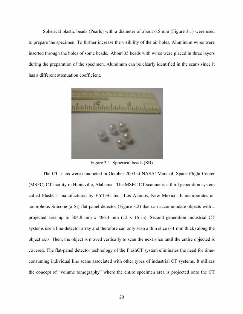
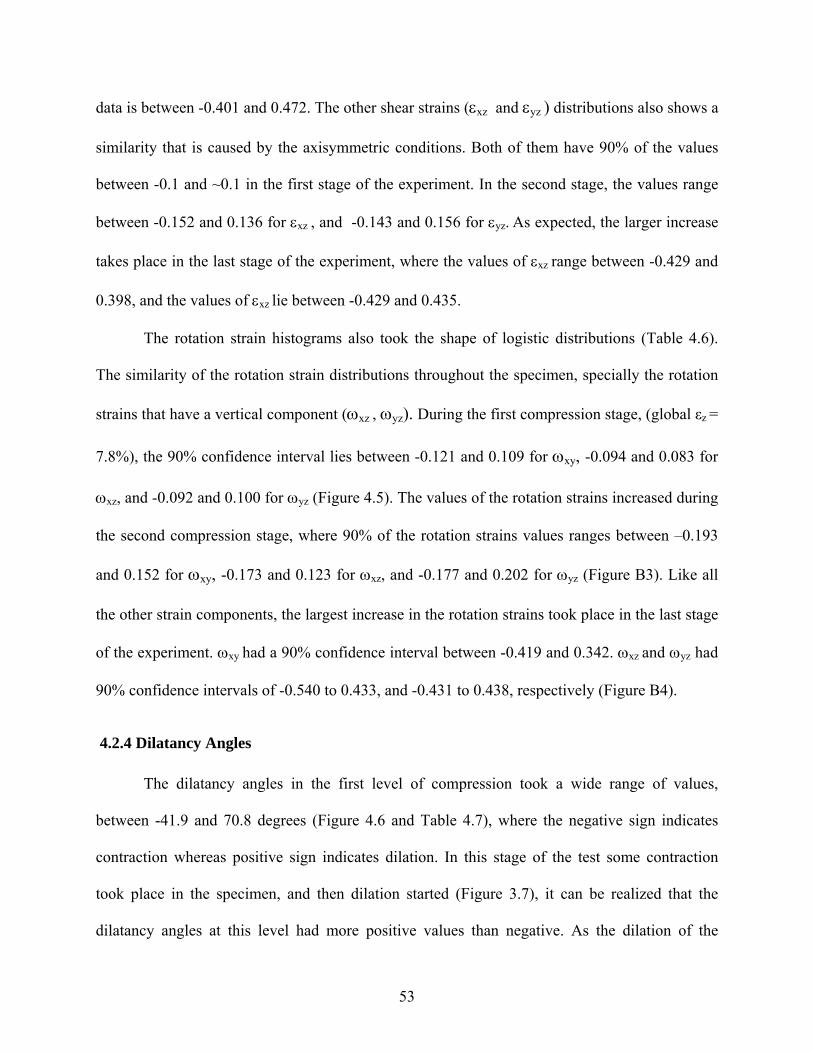
Spherical plastic beads (Pearls) with a diameter of about 6.5 mm (Figure 3.1) were used

to prepare the specimen. To further increase the visibility of the air holes, Aluminum wires were

inserted through the holes of some beads. About 35 beads with wires were placed in three layers

during the preparation of the specimen. Aluminum can be clearly identified in the scans since it

has a different attenuation coefficient.

Figure 3.1. Spherical beads (SB)

The CT scans were conducted in October 2003 at NASA/ Marshall Space Flight Center

(MSFC) CT facility in Huntsville, Alabama. The MSFC CT scanner is a third generation system

called FlashCT manufactured by HYTEC Inc., Los Alamos, New Mexico. It incorporates an

amorphous Silicone (a-Si) flat panel detector (Figure 3.2) that can accommodate objects with a

projected area up to 304.8 mm x 406.4 mm (12 x 16 in). Second generation industrial CT

systems use a line-detector array and therefore can only scan a thin slice (~1 mm thick) along the

object axis. Then, the object is moved vertically to scan the next slice until the entire objected is

covered. The flat-panel detector technology of the FlashCT system eliminates the need for time-

consuming individual line scans associated with other types of industrial CT systems. It utilizes

the concept of “volume tomography” where the entire specimen area is projected onto the CT

20

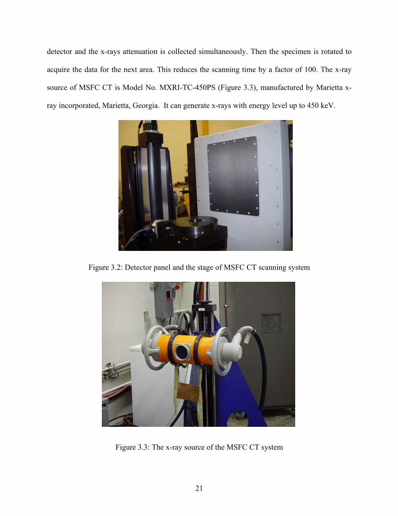
detector and the x-rays attenuation is collected simultaneously. Then the specimen is rotated to

acquire the data for the next area. This reduces the scanning time by a factor of 100. The x-ray

source of MSFC CT is Model No. MXRI-TC-450PS (Figure 3.3), manufactured by Marietta x-

ray incorporated, Marietta, Georgia. It can generate x-rays with energy level up to 450 keV.

Figure 3.2: Detector panel and the stage of MSFC CT scanning system

Figure 3.3: The x-ray source of the MSFC CT system

21

A cylindrical specimen was prepared using the plastic beads (Figure 3.4). The specimen

was held under constant vacuum confinement of 25 kPa. Since the objective of this study is to

study particles’ interaction, only the middle portion of the specimen was scanned. The Specimen

was labeled with two small Aluminum plates that were attached to the membrane surface. They

serve as spatial references for the CT images. The scanning window was kept constant for all

scans performed on the specimen. Before each scan, a 12.7 mm (1/2 in) acrylic rod was attached

to the specimen. It helps to calibrate the density of the specimen for various scans since the CT

reconstruction software tends to change the CT number from one scan volume to another. Four

CT scans were performed on the specimen at different strain levels. First, the specimen was

scanned before compression ( zε = 0%) using 100 keV energy at 1.8 mA current. Then, the

acrylic rod was removed, the test cell was assembled and the specimen was compressed using the

GeoJac loading system (Figure 3.5). The loading was then paused, and the CT scanning was

performed. The process was repeated for the following two scans. It took approximately 10

minutes to scan the volume between the two Aluminum plates for each case. Post scan data

processing took approximately 5 hours/scan producing about 570 slices per scan. Table 3.1

shows the initial dimensions of the specimen and the axial strain level at each CT scan, and

Figure 3.6 shows the location of each CT scan on the stress-strain curve. Figure 3.7 shows the

axial strain versus volumetric strain for the specimen. Load oscillations can be seen in both

figures 3.6 and 3.7, this is due to a slip-stick mechanism that takes place when shearing this type

of particles.

22

Aluminum plates

Figure 3.4. The specimen before compression

Figure 3.5. The specimen in preparation for compression on the stage of CT scanner

23

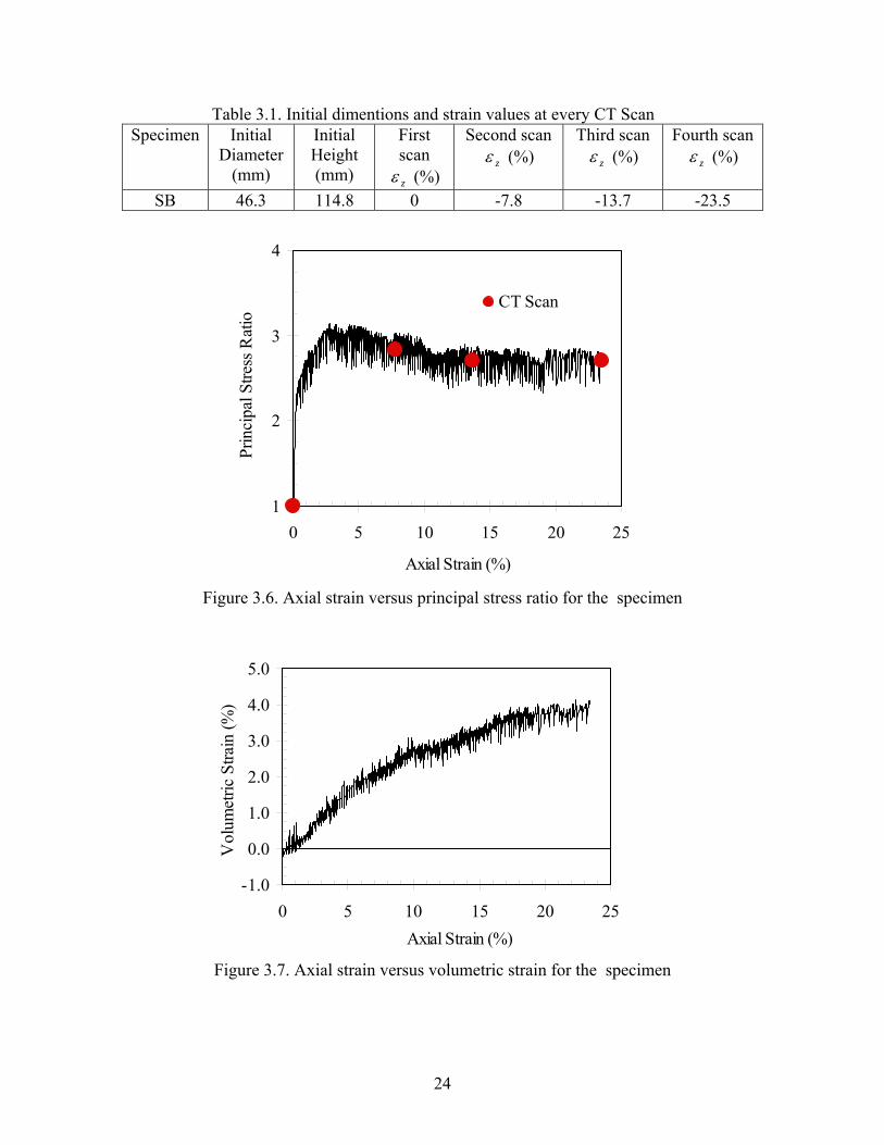
Table 3.1. Initial dimentions and strain values at every CT Scan Specimen Initial

Diameter (mm)

Initial Height (mm)

First scan zε (%)

Second scan zε (%)

Third scan zε (%)

Fourth scan zε (%)

SB 46.3 114.8 0 -7.8 -13.7 -23.5

1

2

3

4

0 5 10 15 20 25

Axial Strain (%)

Prin

cipa

l Stre

ss R

atio

CT Scan

Figure 3.6. Axial strain versus principal stress ratio for the specimen

-1.0

0.0

1.0

2.0

3.0

4.0

5.0

0 5 10 15 20 25Axial Strain (%)

Vol

umet

ric S

train

(%)

Figure 3.7. Axial strain versus volumetric strain for the specimen

24

3.3 VIEWING THE CT IMAGES AND DATA COLLECTION

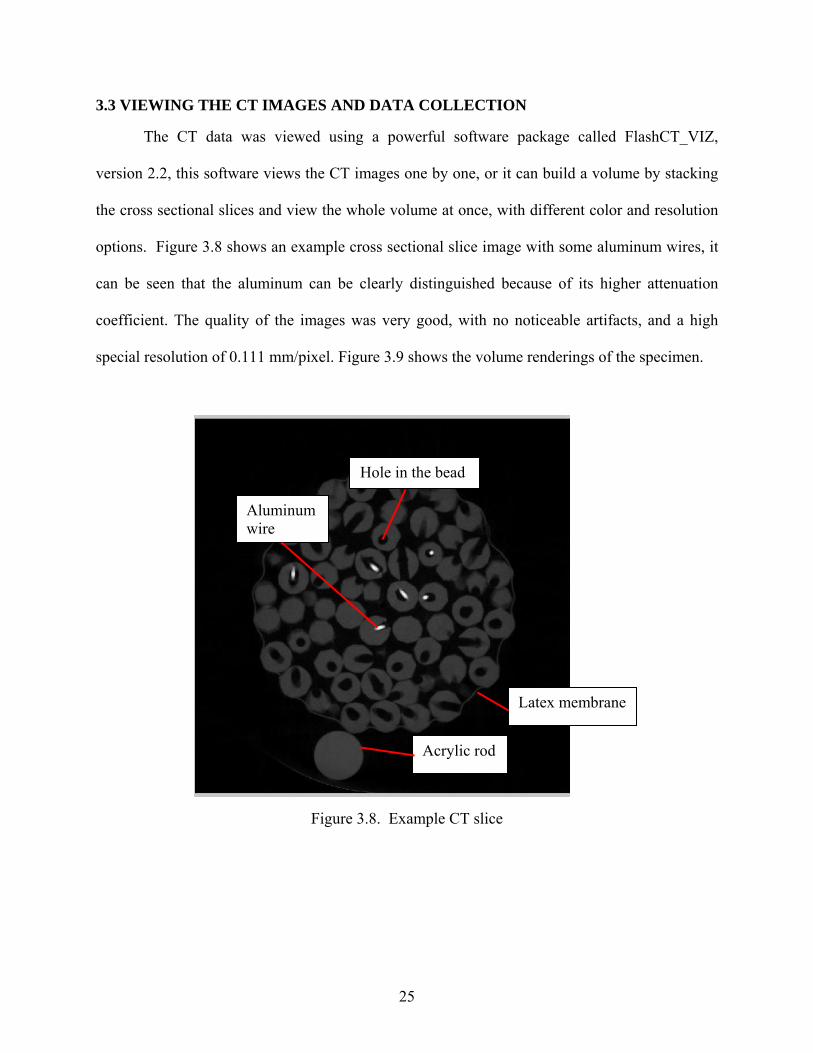
The CT data was viewed using a powerful software package called FlashCT_VIZ,

version 2.2, this software views the CT images one by one, or it can build a volume by stacking

the cross sectional slices and view the whole volume at once, with different color and resolution

options. Figure 3.8 shows an example cross sectional slice image with some aluminum wires, it

can be seen that the aluminum can be clearly distinguished because of its higher attenuation

coefficient. The quality of the images was very good, with no noticeable artifacts, and a high

special resolution of 0.111 mm/pixel. Figure 3.9 shows the volume renderings of the specimen.

Aluminum wire

Hole in the bead

Latex membrane

Acrylic rod

Figure 3.8. Example CT slice

25

(a) zε = 0% (b) zε = -7.8%

(c) zε = -13.7% (d) zε = -23.5%

Figure 3.8. CT volume renderings of the specimen

26

The next step is to track the locations of each particle throughout the four scans; this is a

tedious process that requires a lot of time because it had to be done manually. Since, human

judgment was needed in this process, writing a computer program to perform this job was not a

feasible option. First, cross sections that have the same particles must be identified in the four

volumes; this is achieved by marking a small formation of particles in one scan, and searching

the other scans for a similar formation. And then, particles are numbered such that the same

particle has the same number in the four scans. Figure 3.10 shows four cross sections containing

the same particles taken from four different scans, and the numbering of the particles in each

cross section. Then, the coordinates of the air hole (or the aluminum wire) in each hole must be

recorded. The air hole of each particle is followed by stepping through consecutive slices until

the end point is identified. The x, y and z coordinates of the end point were recorded. Then,

coordinates of the other end point of the particle were identified following the same procedure.

The accuracy of the recorded coordinates is checked by calculating the distance between the end

points of the particle; the distance should be equal to the diameter of the particle. This procedure

was performed for nearly all the particles in the scanned volume (400 particles) to be able to

perform an accurate statistical analysis on the results.

• Translation and Rotation Calculations

The coordinates of the centroid of a particle were calculated as the mean value of its hole

start and end coordinates. Having the coordinates of the center of the particle in the four scans,

the translation in any direction can be calculated as the difference between the location of the

centroid in one scan, and its location in the other scans (Equations 3.1 – 3.3), and the total

distance traveled by the particle can be calculated using Equation 3.4.

27

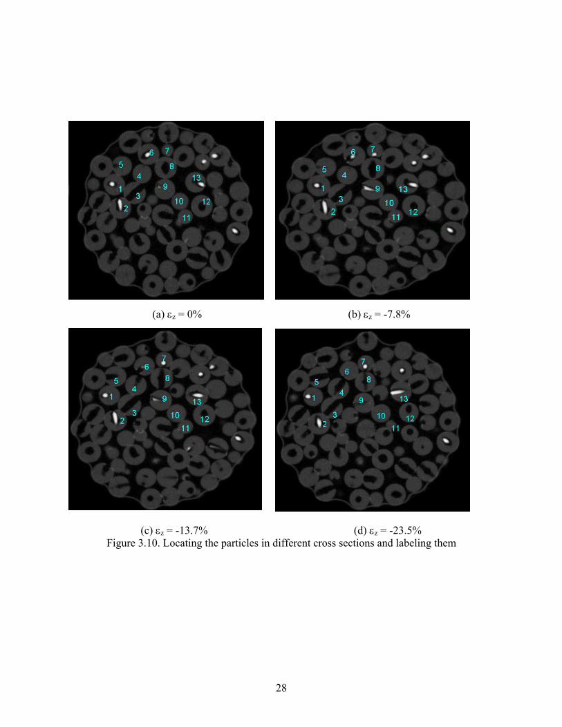
(a) εz = 0% (b) εz = -7.8%

(c) εz = -13.7% (d) εz = -23.5% Figure 3.10. Locating the particles in different cross sections and labeling them

28

∆x = x(scan 2) - x(scan 1) ………………………………………… (3.1)

∆y = y(scan 2) - y(scan 1) ………………………………………… (3.2)

∆z = z(scan 2) - z(scan 1) …………………………………………. (3.3)

D = ∆x2 + ∆y2 + ∆z2 ………………………………………… (3.4)

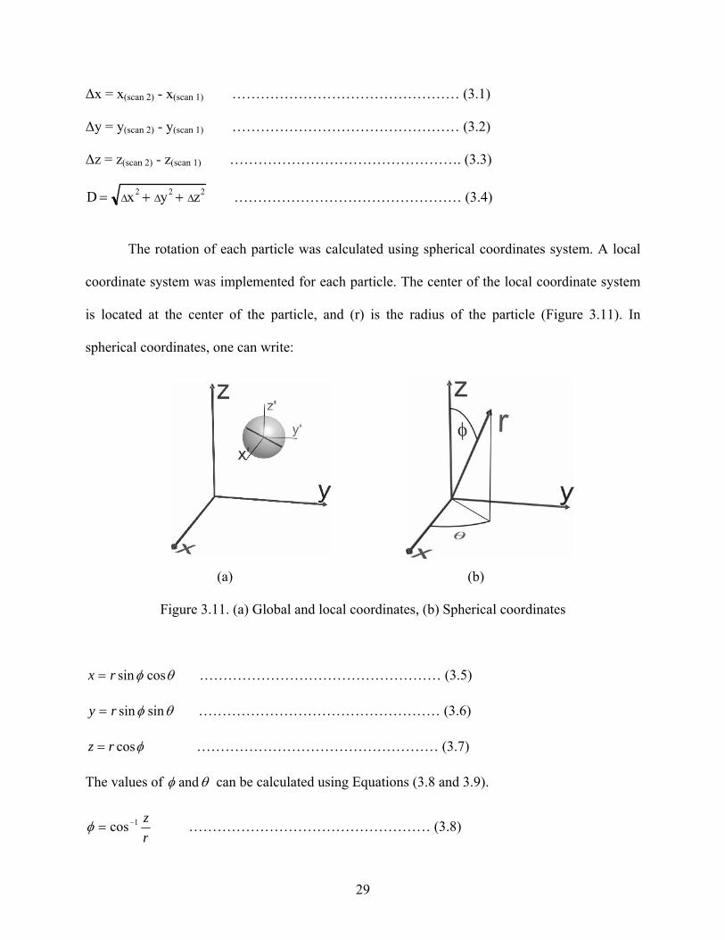
The rotation of each particle was calculated using spherical coordinates system. A local

coordinate system was implemented for each particle. The center of the local coordinate system

is located at the center of the particle, and (r) is the radius of the particle (Figure 3.11). In

spherical coordinates, one can write:

(a) (b)

Figure 3.11. (a) Global and local coordinates, (b) Spherical coordinates

θφ cossinrx = …………………………………………… (3.5)

θφ sinsinry = …………………………………………… (3.6)

φcosrz = …………………………………………… (3.7)

The values of θφ and can be calculated using Equations (3.8 and 3.9).

rz1cos−=φ …………………………………………… (3.8)

29

xy1tan−=θ …………………………………………… (3.9)

The rotation of the particles was taken to be the change in θφ and angles, where the

change in φ is considered to be the vertical component of the rotation, and the change in θ is

the horizontal component of the rotation.

• Local strains

Wang et al. (1999) proposed a finite element based approach to calculate the local strains

resulting from rutting in asphalt concrete. 2D digital images of predefined cross sections were

used to compare the positions of aggregates at different loading levels. A similar method was

used to calculate the local strains in the beads specimen. Modifications were introduced to

account for the third dimension, since, unlike digital images, 3D data is obtained during the CT

scanning process.

The finite element definition of a linear displacement field is presented in Equations 3.10

through 3.12.

zayaxaau 3210 +++= …………………………………………… (3.10)

zbybxbbv 3210 +++= …………………………………………… (3.11)

zcycxccw 3210 +++= …………………………………………… (3.12)

Where: u = the displacement in the x direction.

v = the displacement in the y direction.

w = the displacement in the z direction.

x,y,z = the coordinates of the point in the image.

This definition of the displacement field was used to describe the displacement of the

particles in the specimen. u is equal to ∆x, v is equal to ∆y, w is equal to ∆z. x,y,z were taken as

30

the coordinates of the centroid of the particle. Four coefficients are present in each Equation,

therefore, four particles were considered each time to represent the initial condition. This was

done by selecting the three closest particles (j,k,l) to particle (i). Distances from the center of

particle (i) to the centers of all the other particles were calculated using Equation (3.4). Then the

closest three particles were selected as the particles with the minimum distances from the center

of particle (i). Having the coordinates and displacements of four particles, the system of

equations can be written in a matrix form (Equation 3.13).

1

1

1

1

xi

xj

xk

xl

yi

y j

yk

yl

zi

zj

zk

zl

⎛⎜⎜⎜⎜⎜⎝

⎞

⎟⎟⎟

⎠

a0

a1

a2

a3

⎛⎜⎜⎜⎜⎜⎝

⎞

⎟⎟⎟

⎠

⋅

ui

u j

uk

ul

⎛⎜⎜⎜⎜⎜⎝

⎞

⎟⎟⎟

⎠

……………………………………….. (3.13)

Where, x,y and z denote the coordinates of the centroid; i,j,k and l denote particles.

This system was solved to obtain the “a” coefficients. Then, the same procedure was

repeated to calculate the “b” and “c” coefficients using the v and w displacement fields,

respectively. A computer program was written using MATHCAD software to perform this

analysis. The input for the program was the coordinates of the centroid of all particles in two

scans. For every particle, the distances from the centroids of all the other particles to the centroid

of the particle are calculated, and the closest three particles are selected. Systems of equations

similar to the one presented in Equation (3.13) were solved for the a`s , b`s , and c`s.

The program calculates the strain values using Equations (3.14 – 3.22). This procedure is

repeated for all the particles in the volume, yielding a large number of local strain values that

allows for performing a representative statistical analysis for the local strains distributions.

31

1axu

x =∂∂

=ε …………………………………………….. (3.14)

2byv

y =∂∂

=ε ………………………………………………..(3.15)

3czw

z =∂∂

=ε ………………………………………………..(3.16)

2212 bax

vyu

xy+

=⎟⎟⎠

⎞⎜⎜⎝

⎛∂∂

+∂∂

=ε …………………………………..(3.17)

2213 cax

wzu

xz+

=⎟⎠⎞

⎜⎝⎛

∂∂

+∂∂

=ε ……………………….…………..(3.18)

2223 cby

wzv

yz+

=⎟⎟⎠

⎞⎜⎜⎝

⎛∂∂

+∂∂

=ε ……………………….…………..(3.19)

2212 bax

vyu

xy−

=⎟⎟⎠

⎞⎜⎜⎝

⎛∂∂

−∂∂

=ω ……………………….…………..(3.20)

2213 cax

wzu

xz−

=⎟⎠⎞

⎜⎝⎛

∂∂

−∂∂

=ω …………...………….…………..(3.21)

2223 cby

wzv

yz−

=⎟⎟⎠

⎞⎜⎜⎝

⎛∂∂

−∂∂

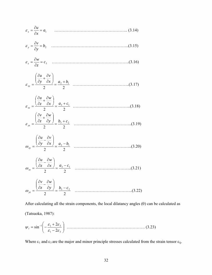
=ω ……………………….…………..(3.22)

After calculating all the strain components, the local dilatancy angles (θ) can be calculated as

(Tatsuoka, 1987):

⎟⎟⎠

⎞⎜⎜⎝

⎛−+

−= −

31

311

22

sinεεεε

ψ l ………………………..………………………. (3.23)

Where ε1 and ε3 are the major and minor principle stresses calculated from the strain tensor εij.

32

Tatsuoka (1987) suggested Equation (3.23) for axisymmetric triaxial compression based on

comparison of laboratory measurements of plane strain and axisymmetric triaxial

compression experiments.

(dεv / dε1)

• 3D Visualization

After obtaining the coordinates of all the particles, they were used to generate 3D

renderings of the particles. Figures 3.12 through 3.15 show multiple views of a cluster of eight

particles at four different compression stages. And Figures 3.16 through 3.18 show multiple

views on individual beads at the four compression stages. It is also possible to create 3D

animations showing the movement of the particles throughout the experiment.

33

(a) x-z view (front view)

(b) x-y view (top view)

Figure 3.12. 3D rendering of a cluster of particles before compression (

zε = 0%)

34

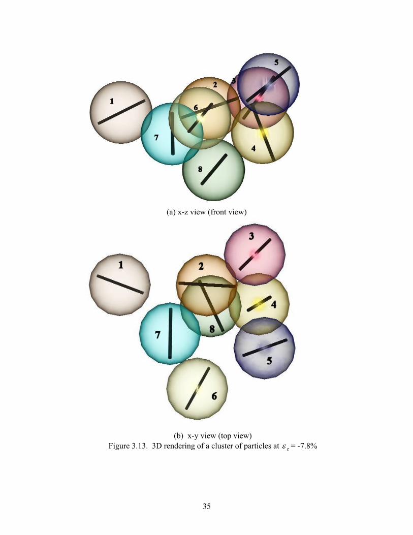
(a) x-z view (front view)

(b) x-y view (top view) Figure 3.13. 3D rendering of a cluster of particles at zε = -7.8%

35

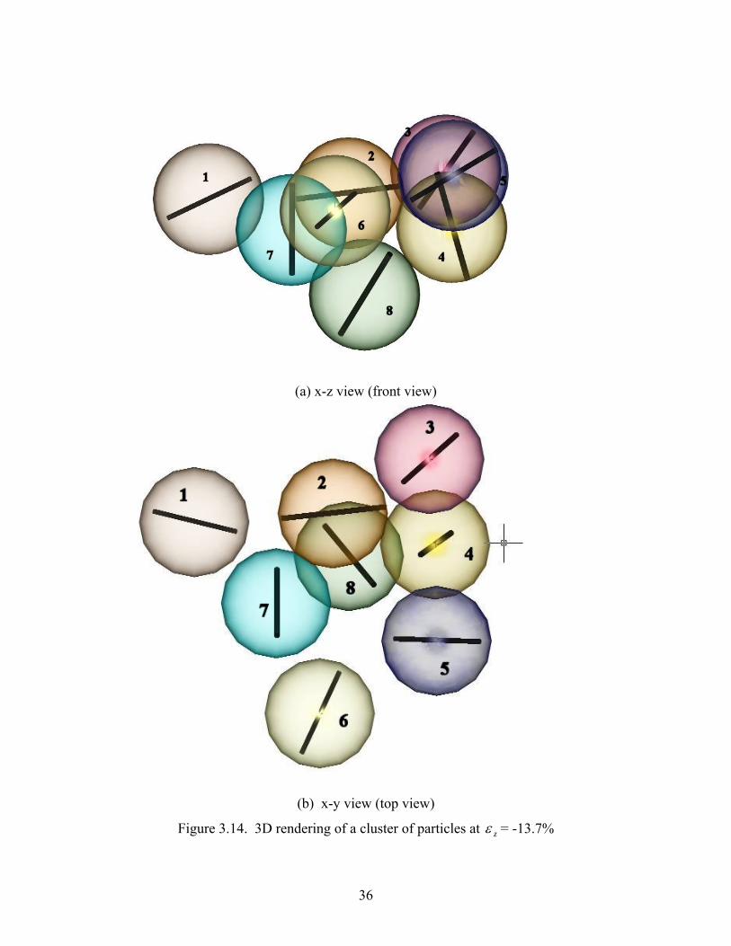
(a) x-z view (front view)

(b) x-y view (top view)

Figure 3.14. 3D rendering of a cluster of particles at

zε = -13.7%

36

(b) x-y view (top view)

Figure 3.15. 3D rendering of a cluster of particles at

(a) x-z view (front view)

zε = -23.5%

37

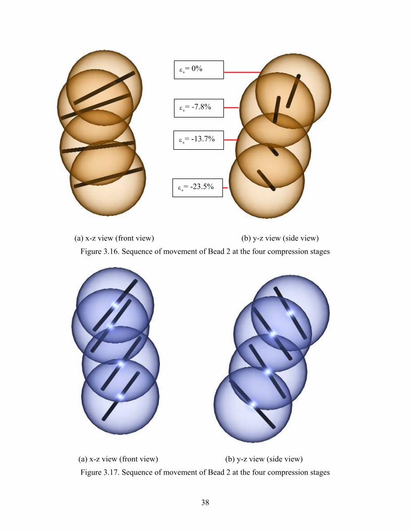
(a) x-z view (front view) (b) y-z view (side view)

Figure 3.16. Sequence of movement of Bead 2 at the four compression stages

(b) y-z view (side view)

Figure 3.17. Sequence of movement of Bead 2 at the four compression stages

= -13.7% εa

εa= 0%

εa= -7.8%

εa= -23.5%

(a) x-z view (front view)

38

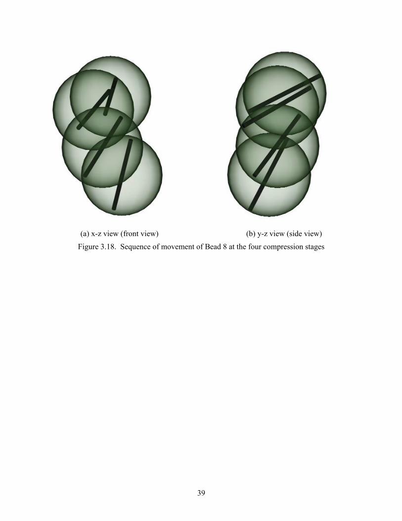
(b) y-z view (side view)

Figure 3.18. Sequence of movement of Bead 8 at the four compression stages

(a) x-z view (front view)

39

CHAPTER FOUR

RESULTS AND DISCUSSION

.1 RESULTS

.1.1 Translation and Rotation

The translation and rotation es were calculated as described in

Chapter 3. The data was pre tions. A statistical analysis

as performed, and the data was then fitted to the closest probability density distribution. Then

intervals were calculated.

The Frequency distributions for the translation for the first stage of the experiment are

presented in Figure 4.1, and for the other stages, the figures are presented in Appendix A. Since

the scanning was not performed on uniform strain intervals, the translation values were

normalized with respect to the value of the displacement at the top of the specimen at every stage

of the experiment, and are presented as percentages of that value. It should be noted that the

translation values are not presented in cumulative form, i.e. the presented values represent the

translation that took place between the scan under consideration, and the previous scan. This way

of presentation was selected to make it easier to note the changes in the translation rate that takes

place at different stages throughout the experiment. The values for the horizontal translations (X

and Y directions) were taken as absolute values.

4

4

for four hundred particl

sented in the form of frequency distribu

w

the “90% level of confidence”

• Translation

40

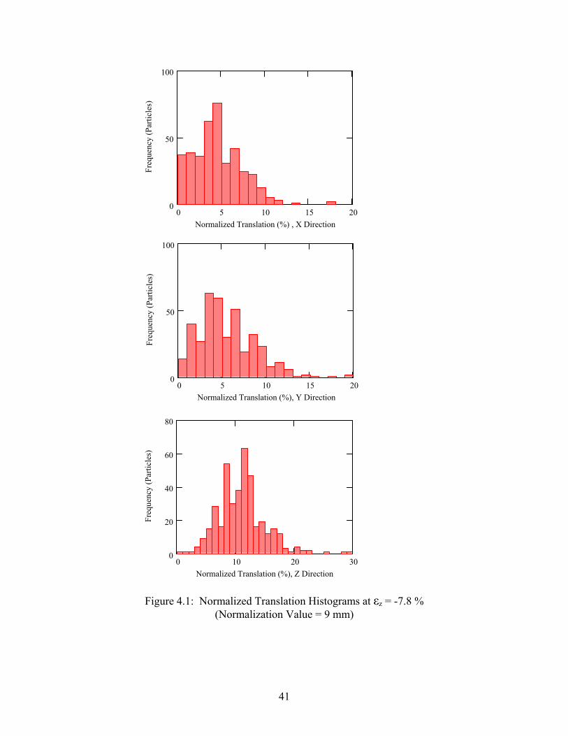
Figure 4.1: Normalized Translation Histograms at εz = -7.8 %

(Normalization Value = 9 mm)

0 5 10 15 200

50

100

Normalized Translation (%) , X Direction

Freq

uenc

y (P

artic

les)

0 5 10 15 200

50

100

Normalized Translation (%), Y Direction

Freq

uenc

y (P

artic

les)

0 10 20 300

20

40

60

80

Normalized Translation (%), Z Direction

Freq

uenc

y (P

artic

les)

41

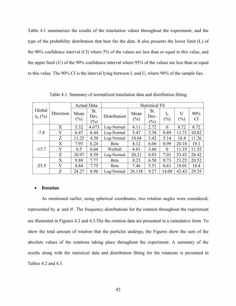
Table 4.1 summarizes the results of the translation values throughout the experiment, and the

pe of the probability distribution that best fits the data. It also presents the lower limit (L) of

the 90% confidence interval (CI) where 5% of the values are less than or equal to this value, and

the upper limit (U) of the 90% co the values are less than or equal

this value. The 90% CI is the interval lying between L and U, where 90% of the sample lies.

ty

nfidence interval where 95% of

to

Table 4.1. Summary of normalized translation data and distribution fitting

Actual Data Statistical Fit Global St.

(%)

St.

(%) εz (%) Direction Mean

(%) Dev. Distribution Mean (%) Dev. L

(%) U

(%) 90% CI

X 5.32 4.673 Log-Normal 4.11 2.72 0 8.72 8.72 Y 6.47 6.44 Log-Normal 5.47 3.38 0.89 11.71 10.82-7.8 Z 11.25 4.50 Log-Normal 10.68 3.42 5.14 16.4 11.26X 7.93 6.24 Beta 8.12 6.06 0.99 20.16 19.1 Y 6.5 6.66 Weibull 4.61 3.60 0 11.35 11.35-13.7 Z 20.97 8.59 Log-Normal 20.21 8.03 7.01 33.43 26.42X Beta 8.23 73 21.25 20.529.88 7.77 6.50 0.Y 8.84 7.75 Beta 5.51 0.61 19.01 18.4 7.46 -23.5 Z 24.27 8.96 Log-Normal 26.138 14.08 43.43 29.359.27

• tation

As mentioned earlier, using spherical coordinat o n s o ed,

represented by

Ro

es, tw rotatio angle were c nsider

φ and θ . The fre y f ot th o ent

are illustrated in Figures 4.2 and e the ion da pre d m

w the total amount of rotation that the particles undergo, the Figures show the sum of the

absolute values of the rotations taking place throughout the experiment. A summary of the

results

quenc distributions or the r ation rough ut the experim

4.3.Th rotat ta are sente in a cu ulative form. To

sho

along with the statistical data and distribution fitting for the rotations is presented in

Tables 4.2 and 4.3.

42

Figure 4.2. φ Angle rotation throughout the experiment

Table 4.2. Statistical summary of rotation angleφ

Actual Data Statistical Fit

εz (%) Dev (

Distribution Me(degree.) (degree) (degree.) (degree.)

0% CI (degree)

Mean (degree)

Std.

degree)

an St. Dev. L U 9

-7.8 -0.074 4.62 9.51 4.74 Normal -0.13 2.93 -4.89 -13.7 -0.93 8.79 Normal -0.76 4.67 -8.40 6.90 15.3 -23.5 -2.34 11.46 Normal -2.00 11.46 -17.10 13.09 30.19

0 10 20 30 400

10

20

30

40Fr

eque

ncy

(Par

ticle

s)

φ Absolute Cumulative Rotation (degree)

φ Angle Rotation (degree) (a) εz = -7.8 %

10 5 0 5 100

20

60

40

Freq

uenc

y (P

artic

les)

φ Angle Rotation (degree) (b) εz = -13.7%

10 5 0 5 100

20

40

60

Freq

uenc

y (P

artic

les)

φ Angle Rotation (degree) (c) εz = -23.5 %

20 10 0 10 200

10

30

20

Freq

uenc

y (P

artic

les)

43

44

θ Angle Rotation (degree) (a) εz = -7.8 %

θ Angle Rotation (degree) (b) εz = -13.7 %

θ Angle Rotation (degree) (c) εz = -23.5 %

θ Angle Cumulative Rotation (degree)0 20 40 60

0

10

20

30

Freq

uenc

y (P

artic

les)

40 20 0 20 400

10

20

30

40

Freq

uenc

y (P

artic

les)

30

40

60

80

20 10 0 10 20 300

20Freq

uen

30

cy (P

artic

les)

20 10 0 10 20 300

20

80

40

60

Freq

uenc

y (P

artic

les)

Figure 4.3:

θ angle rotation throughout the experiment

Table 4.3: Statistical summary of rotation angleθ Actual Data Statistical Fit

εz (%) Mean

(degree.)

Std. Dev

(degree) Distribution Mean

(degree)St. Dev. (degree)

L (degree)

U (degree)

90% CI (degree)

-7.8 0.51 7.63 Normal 0.75 4.91 -7.22 8.73 15.95 -13.7 1 al 0.69 .16 11.92 Norm 7.60 -11.8 13.2 25 -23.5 al 1.46 16.26 1.66 20.85 Norm -25.3 28.2 53.5

4.1.2 Local

The local strains are calculated using the me h r

(Equations 3.14 through 3.22). The results for the first stage of the experime pre in

Strains

thod described in t e previous Chapte

nt are sented

45

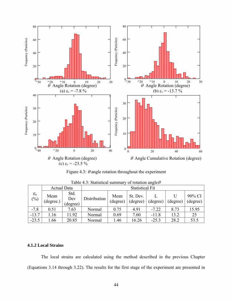
cy di tions he r or th owing ges

are presented in Appendix B. Cumulative values of the axial and radial strains (εz, εx and εy),

shear strains (εxy, εxz, and εyz), and rotation strains(ωxy, ωxz, and ωyz) at the different stages on the

nted in each Figure. Then a summary of the results along with the best fit

frequen

Figure 4.4. Local strains histograms at εz = -7.8%

Figures 4.4 and 4.5 in the form of frequen stribu , and t esults f e foll sta

experiment are prese

cy distribution and the confidence intervals are shown in Tables 4.4, 4.5 and 4.6.

εz

0.4 0.2 0 0.2 0.40

20

40

60

80

Freq

uenc

y (P

artic

les)

εx0.4 0.2 0 0.2 0.4

20

40

0

Freq

uenc

y (P

artic

les)

εy0.4 0.2 0 0.2 0.4

20

0

40

Fre

ncy

(Pa

ticle

s)qu

er

εxy0.4 0.2 0 0.2 0.4

0

20

40

60

Freq

uenc

y (P

artic

les)

εxz0.4 0.2 0 0.2 0.4

0

20

40

60

Freq

uenc

y (P

artic

les)

ε0.4 0.2 0 0.2 0.4

0

20

40

60

Freq

uenc

y (P

artic

les)

yz

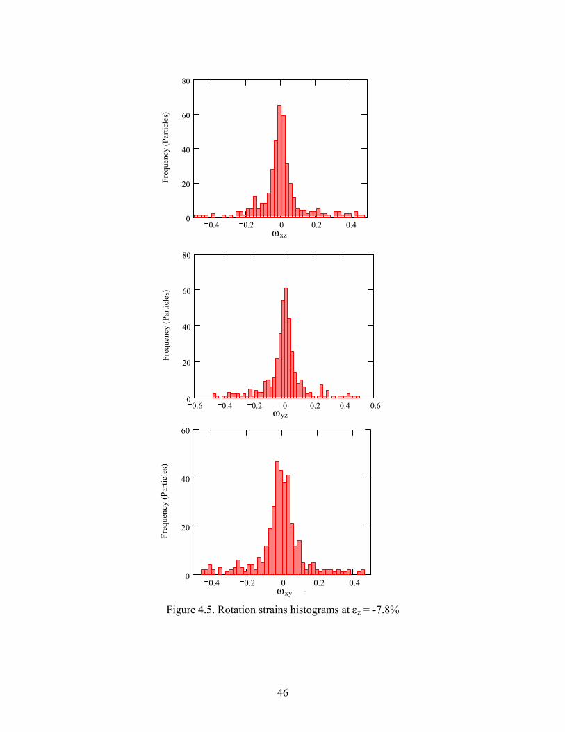
Figure 4.5. Rotation strains histograms at εz = -7.8%

ωyz0.6 0.4 0.2 0.2 0.4 0.6

0

20

40

60

80

0

Freq

uenc

y (P

artic

les)

yzω

0.4 0.2 0 0.2 0.4

20

40

60

80

0

Freq

uenc

y (P

artic

les)

ω xzωxz

0.4 0.2 0.2 0.40

20

40

60

0

Freq

uenc

y (P

artic

les)

ω xyωxy

46

Table 4.4: Summary of axial and radial strains data and distribution fitting

Actual Data Statistical Fit Global εz (%) Component Mean St.

Dev. Distributi

on Mean St. Dev. L U 90%

CI εx 0.026 0.15 Log-

Norm 0.065 0.10 -0.045 0.262 0.307al εy Log- 0.359 0.3960.014 0.15 Normal 0.089 0.15 -0.037 -7.8

εz -0.014 0.08 Normal -0.013 0.04 -0.080 0.055 0.135εx 0.041 0.16 Log

Normal 0.056 0.12 -0.115 0.275 0.390-

εy 0.035 0.15 Log-Normal 0.053 0.10 -0.089 0.223 0.312-13.7

εz -0.016 0.14 Normal 0.012 5 0.09 0.205 0.06 -0.11εx 0.085 0 0 -0.240 0.611 .32 Log-

Normal 0.133 .26 0.851

εy 0.070 0.36 Log-Normal 0.140 0.27 -0.244 0.621 0.865-23.5

0.002 0.39 -0.049 0.19 -0.358 0.259 0.617εz Logistic

ble 4.5 ary of sh s data and distribution fitting Ta : Summ ear strain

Actual Data Statistical Fit Global εz

(%) Com nt

D Distribution pone

Mean St. ev. Mean St.

Dev. L U 90% CI

εxy 0.006 0.14 Logistic 0.003 0.07 -0.104 0.111 0.215ε -0.013 0.13 xz Logistic -0.006 0.06 -0.101 0.088 0.189-7.8

-0.007 0.12 Logistic εyz 0.000 0.06 -0.100 0.100 0.200εxy 0.010 0.16 Logistic 0.01 0.09 -0.133 0.150 0.283εxz -0.002 0.15 Logistic -0.008 0.09 -0.152 0.136 0.288-13.7 εyz -0.001 0.14 Logistic 0.007 0.09 -0.143 0.156 0.299εxy 0.036 0.35 Logistic 0.031 0.27 -0.409 0.472 0.881εxz 0.002 0.36 Logistic -0.015 0.25 -0.429 0.398 0.827-23.5 εyz Logistic 0.003 9 0.435 0.8640.020 0.38 0.27 -0.42

47

T le 4.6: ar ota s d u i

Actual Data Statistical Fit

ab Summ y of r tion strain ata and distrib tion fitt ng

Global εz

(%) Component

Mean St. Dev. Distribution Mean St.

Dev. L U 90% CI

ωxy -0.015 0.13 Logistic -0.006 0.07 -0.121 0.109 0.230ωxz -0.001 0.13 Logistic -0.006 0.05 -0.094 0.083 0.177-7.8 ωyz -0.003 0.13 Logistic 0.004 0.06 -0.092 0.100 0.192ωxy -0.022 0.15 Logistic -0.020 0.11 -0.193 0.152 0.345ωxz -0.023 0.15 Logistic -0.025 0.10 -0.173 0.123 0.296-13.7 ωyz 0.015 0.15 Logistic 0.012 0.12 -0.177 0.202 0.379ωxy -0.007 0.34 Logistic -0.038 0.23 -0.419 0.342 0.761ωxz -0.018 0.38 Logistic -0.054 0.30 -0.540 0.433 0.973-23.5 ω Logistic 0.004 1 0.438 0.869yz 0.046 0.40 0.27 -0.43

4.1.3 Dilatancy Angles

The loc latanc s lcu ng n . s cal

dila ngle gram d nt the m a the

results as well a stat t ation are shown in Table 4.7.

.2 DISCUSSIO OF R TS

4.2.1 Translation

The translation values in the lateral direction (x and y) and axial direction (z) were studied with

the aid of Figures 4.1, A1, and A2 (Appendix A) and Table 4.1. The lateral translation during the

first stage of the experiment (ε = -7.8%) looks similar in the x and y directions, a mean value of

5.3% of the displacement at top of the specimen was obtained in the x direction, and a value of

6.5% was obtained in the y direction (Figure 4.1). It is also realized that the shapes of the

histograms in x and y direction look similar. This is due to the axisymmetric conditions of the

experiment.

al di y angle are ca lated usi Equatio 3.23. Figure 4 6 show the lo

tancy a histo s at the iffere stages of experi ent. A statistic l summary of

s the istical fi inform

4 N ESUL

z

48

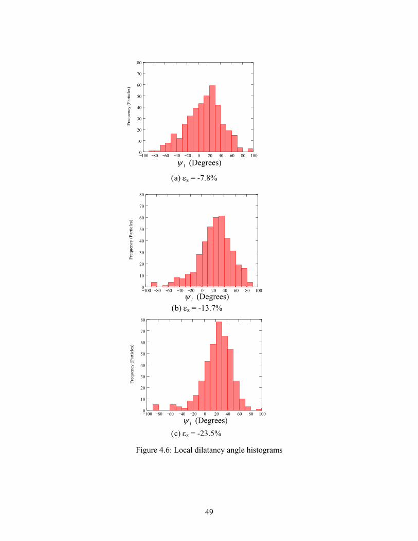
Figure 4.6: Local dilatancy angle histograms

100 80 60 40 20 0 20 40 60 80 1000

10

20

30

40

50

60

70

80

Freq

uenc

y (P

artic

les)

lψ (Degrees)

100 80 60 40 20 0 20 40 60 80 1000

10

20

30

40

50

60

70

80

Freq

uenc

y (P

artic

les)

lψ (Degrees)

(a) εz = -7.8%

(c) εz = -23.5%

(b) εz = -13.7%

lψ (Degrees) 100 80 60 40 20 0 20 40 60 80 100

0

10

20

30

50

40

60

70

80

Frs)

eque

ncy

(Par

ticle

49

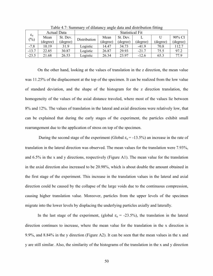
Table 4.7: SActual Data

ummary of dilatancy angle data and distribution fitting Statistical Fit εz

(%) Mean (degree)

U (degree)

90% CI (degree)

St. Dev. (degree) Distribution Mean

(degree) St. Dev. (degree)

L (degree)

-7.8 10.19 -41.9 70.8 112.7 31.9 Logistic 14.47 34.73 -13.7 22.85 30.8 -21.7 75.5 97.2 7 Logistic 26.87 29.93 -23.5 21.68 26.5 -12.6 65.3 77.9 3 Logistic 26.34 23.97

On the other hand, looking at the values of translation in the z direction, the mean value

as 11.25% of the displacement at the top en. It can be realized from the low value

f standard deviation, and the sha gram for the z direction translation, the

homogeneity of the values of the axial distance here most of the values lie between

8% and 12%. The values of translation in the lateral and axial directions were relatively low, that

can be explained that during the early stages of the e particles exhibit small

re ge t li s f im

Du e se tage peri lo -13 n inc in th of

anslation in the lateral direction was observed. The mean values for the translation were 7.93%,

and 6.5

e translation in the lateral

directio

w of the specim

o pe of the histo

traveled, w

experiment, th

arran ment due o the app cation of stre s on top o the spec en.

ring th cond s of the ex ment (G bal εz = .5%) a rease e rate

tr

% in the x and y directions, respectively (Figure A1). The mean value for the translation

in the axial direction also increased to be 20.98%, which is about double the amount obtained in

the first stage of the experiment. This increase in the translation values in the lateral and axial

direction could be caused by the collapse of the large voids due to the continuous compression,

causing higher translation value. Moreover, particles from the upper levels of the specimen

migrate into the lower levels by displacing the underlying particles axially and laterally.

In the last stage of the experiment, (global εz = -23.5%), th

n continues to increase, where the mean value for the translation in the x direction is

9.9%, and 8.84% in the y direction (Figure A2). It can be seen that the mean values in the x and

y are still similar. Also, the similarity of the histograms of the translation in the x and y direction

50

can still be clearly seen where they both take the shape of a “Beta distribution”. As mentioned

earlier, this is an expected result due the axisymmetric conditions of the experiment. The

translation in the axial direction also increases, to have a mean value of 24.27% and the values in

the 90% level of confidence reach up to 43%. This stage of the experiment is best described as

the critical state, where the shear resistance of the specimen is very small and greater strains can

be gene

As mentioned earlier, a vertical (φ) and a horizontal (θ) component of the rotation were

considered. From Figure 4.2 and Table 4.2, the vertical rotation histograms during all the stages

of the experiment take the shape of normal distributions. During the first stage of the experiment,

90% of the vertical rotation values lie between -4.9 and 4.6 degrees. While in the second stage

they lie between -8.4 and 6.9 degrees. In the final stage of the experiment 90% of the values lie

between -17.1 and 13.1 degrees. Taking the absolute values of all the rotations, the cumulative

vertical rotation values reach up to 30 degrees. On the other hand, the horizontal rotation had

higher values, where 90% of the values of the θ angle rotation in the first stage of the experiment

-7.22 and 8.73 degrees (Figure 4.3). During the second stage, the values lie

betwee

rated with relatively small stresses.

4.2.2 Rotation

range between

n -11.8 and 13.2 degrees. On the final stage of the experiment, the horizontal rotation

values range between -25.3 and 28.2 degrees. Like the vertical rotation, the horizontal rotation

histograms took the shape of normal distributions. Taking the absolute values of all the rotations,

the cumulative horizontal rotation values reach up to 60 degrees.

51

4.2.3 Local Strains

Studying the local strains distributions in Figures 4.4, 4.5 and Appendix B (Figures B1 to

B4), a considerable similarity can be noticed between the lateral strains (εx and εy) throughout the

experiment. They always had a Log-Normal distribution that tends to have more positive values

then negative. The positive sign here indicates dilation, or expansion, and that’s what is expected

to happen during the compression of the specimen, where it expands laterally. During the last

stage of the experiment, it is noted that there is some difference in the shape of the lateral strains

histograms. This happens because the bulging at failure in the middle portion of the specimen

(where the CT scans are taken) is not perfectly symmetric around the z axis. The specimen might

expand laterally in one direction more than the other, but there is an overall similarity between

the lateral stain values, due to the axisymmetry.

On the other hand, the axial strain (ε ) distributions take a normal distribution shape in

the first and second stages of the experiment, the distributions always have a negative mean that

indicates compression, and this is the expected result when axially compressing a specimen. On

the final stage, the negative values dominate, resulting in a Logistic distribution where most of

the values lie in the negative (compression) area. This result indicates the higher values in axial

strains obtained at failure.

All the local shear strains histograms took the shape of a Logistic distribution. The

positive or negative signals for the shear strains only indicate the direction of shearing, and are

not related to the expansion or compression. In the first stage of the experiment 90% of the

values of the horizontal shear strains (ε ) range between -0.104 and 0.111, while in the second

last stage of the experiment, where 90% of the

z

xy

stage they lie between -0.133 and 0.150. An as seen in the axial and lateral stains as well as the

translation, the greatest increase is noted in the

52

data is

strains values ranges between –0.193

xy xz yz

xy xz yz

4.2.4 Dilatancy Angles

The dilatancy angles in the first level of compression took a wide range of values,

between -41.9 and 70.8 degrees (Figure 4.6 and Table 4.7), where the negative sign indicates

contraction whereas positive sign indicates dilation. In this stage of the test some contraction

took place in the specimen, and then dilation started (Figure 3.7), it can be realized that the

dilatancy angles at this level had more positive values than negative. As the dilation of the

between -0.401 and 0.472. The other shear strains (εxz and εyz ) distributions also shows a

similarity that is caused by the axisymmetric conditions. Both of them have 90% of the values

between -0.1 and ~0.1 in the first stage of the experiment. In the second stage, the values range

between -0.152 and 0.136 for εxz , and -0.143 and 0.156 for εyz. As expected, the larger increase

takes place in the last stage of the experiment, where the values of εxz range between -0.429 and

0.398, and the values of εxz lie between -0.429 and 0.435.

The rotation strain histograms also took the shape of logistic distributions (Table 4.6).

The similarity of the rotation strain distributions throughout the specimen, specially the rotation

strains that have a vertical component (ωxz , ωyz). During the first compression stage, (global εz =

7.8%), the 90% confidence interval lies between -0.121 and 0.109 for ωxy, -0.094 and 0.083 for

ωxz, and -0.092 and 0.100 for ωyz (Figure 4.5). The values of the rotation strains increased during

the second compression stage, where 90% of the rotation

and 0.152 for ω , -0.173 and 0.123 for ω , and -0.177 and 0.202 for ω (Figure B3). Like all

the other strain components, the largest increase in the rotation strains took place in the last stage

of the experiment. ω had a 90% confidence interval between -0.419 and 0.342. ω and ω had

90% confidence intervals of -0.540 to 0.433, and -0.431 to 0.438, respectively (Figure B4).

53

specimen continues at the later levels of the experiment, the fraction of positive dilatancy angles

gradually increases, where at the final stage of the test, positive values dominate the dilatancy

angle distribution, and a smaller range of dilatancy angle values were obtained (-12.6 to 65

degrees).

54

CHAPTER FIVE

SPATIAL POROSITY DISTRIBUTION OF ROCK CORES STUDIED BY µCT

.1 INTRODUCTION

In this part of the thesis, CT technology was used to study the porosity distribution of

synthetic rock cores. Several rock co ain size distributions, and prepared

u

umber to the bulk density was conducted, and then the correlation was used to obtain the

porosity distribution for the cores. They were compared to determine the effect of grain size

distribution and consolidation pressure on the local porosity distribution of the cores.

2

The main

rtz powder. The cores were prepared by thoroughly mixing the

s as a cementing agent. Table 5.1 shows a list of the cores along

with their grain size distribution, and the compaction pressure used to prepare them. The cores

have a cylindrical shape, with an average radius of 28 mm and an average height of 29 mm

(Figure 5.1).

5

res having different gr

nder different consolidation pressures were scanned. A density calibration to correlate the CT

n

5.2 EXPERIMENTAL WORK

5.2.1 Specimen Description

Twelve synthetic rock cores were used in this study. The cores were prepared by mixing

Quartz (SiO ) with four classes (Powder, 0.126-0.149 mm, 0.149-0.177 mm, and 0.177-0.210

mm) and consolidating (Compacting) them under 3000, 4000 or 5000 psi pressures.

constituent of the cores is the Qua

particles and adding liquid glas

55

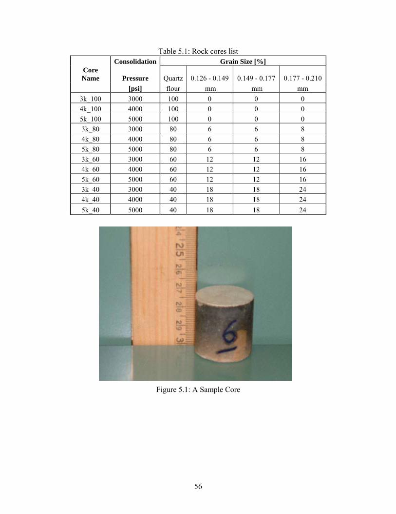
Table 5.1: Rock cores list Consolidation Grain Size [%]

Core Name Pressure Quartz 0.126 - 0.149 0.149 - 0.177 0.177 - 0.210

[psi] flour mm mm mm 3k_100 3000 100 0 0 0 4k_100 4000 100 0 0 0 5k_100 5000 100 0 0 0 3k_80 3000 80 6 6 8 4k_80 4000 6 8 80 6 5k_80 5000 80 6 8 6 3k_60 3000 60 12 12 16 4k_60 4000 60 12 12 16 5k_60 5000 60 12 12 16 3k_40 3000 40 18 18 24 4k_40 4000 40 18 18 24 5k_40 5000 40 18 18 24

Figure 5.1: A Sample Core

56

5.2.2 CT Scanning

The CT scans were performed using the Washington State University CT laboratory in

ugust, 2003, using a system similar to the MSFC CT system (Figure 5.2), with a different x-ray

source. The x-ray was generated using an X-tek 225 kV microfocus x-ray source (Figure 5.3). It

has a 5

A

µm

beam with m

focal spot size x-ray source with microfocus option that can produce an intense x-ray

inimum penumbra. It took approximately 6 minutes to scan each specimen at

keV and 0.158 mA current. The distances from the x-ray source to the

specim

energy level of 142

en and from the specimen to the detector panel were 244.5 and 416 mm, respectively,

producing about 700 slices per core. Each slice is about 620 x 620 pixels yielding a spatial

resolution of about 47.83 µm/pixel. Figure 5.4 shows example CT renderings of one of the

scanned cores.

Figure 5.2. The X-ray CT System of Washington State University (WAX-CT)

57

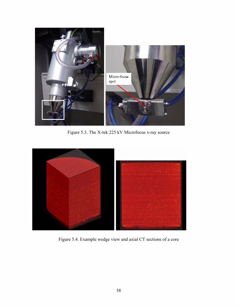
Figure 5.4. Example wedge view and axial CT sections of a core

Figure 5.3. The X-tek 225 kV Microfocus x-ray source

58

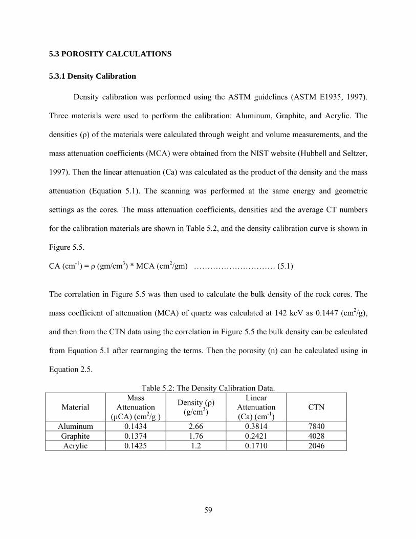
5.3 POROSITY CALCULATIONS

5.3.1 Density Calibration

Density calibration was performed using the ASTM guidelines (ASTM E1935, 1997).

Three materials d Acrylic. The

ensities (ρ) of the materials were calculated through weight and volume measurements, and the

ass attenuation coefficients (MCA) were obtained from the NIST website (Hubbell and Seltzer,

997). Then the linear attenuation (Ca) was calculated as the product of the density and the mass

ed at the same energy and geometric

ass attenuation coefficients, densities and the average CT numbers

for the

The correlation in Figure 5.5 was then used to calculate the bulk density of the rock cores. The

mass coefficient of attenuation (MCA) of quartz was calculated at 142 keV as 0.1447 (cm2/g),

and then from the CTN data using the correlation in Figure 5.5 the bulk density can be calculated

from Equation 5.1 after rearranging the terms. Then the porosity (n) can be calculated using in

Equation 2.5.

Table 5.2: The Density Calibration Data.

Material Attenuation (µCA) (cm2/g ) (g/cm3) Attenuation

(Ca) (cm-1) CTN

were used to perform the calibration: Aluminum, Graphite, an

d

m

1

attenuation (Equation 5.1). The scanning was perform

settings as the cores. The m

calibration materials are shown in Table 5.2, and the density calibration curve is shown in

Figure 5.5.

CA (cm-1) = ρ (gm/cm3) * MCA (cm2/gm) ………………………… (5.1)

Mass Density (ρ) Linear

Aluminum 0.1434 2.66 0.3814 7840 Graphite 0.1374 1.76 0.2421 4028 Acrylic 0.1425 1.2 0.1710 2046

59

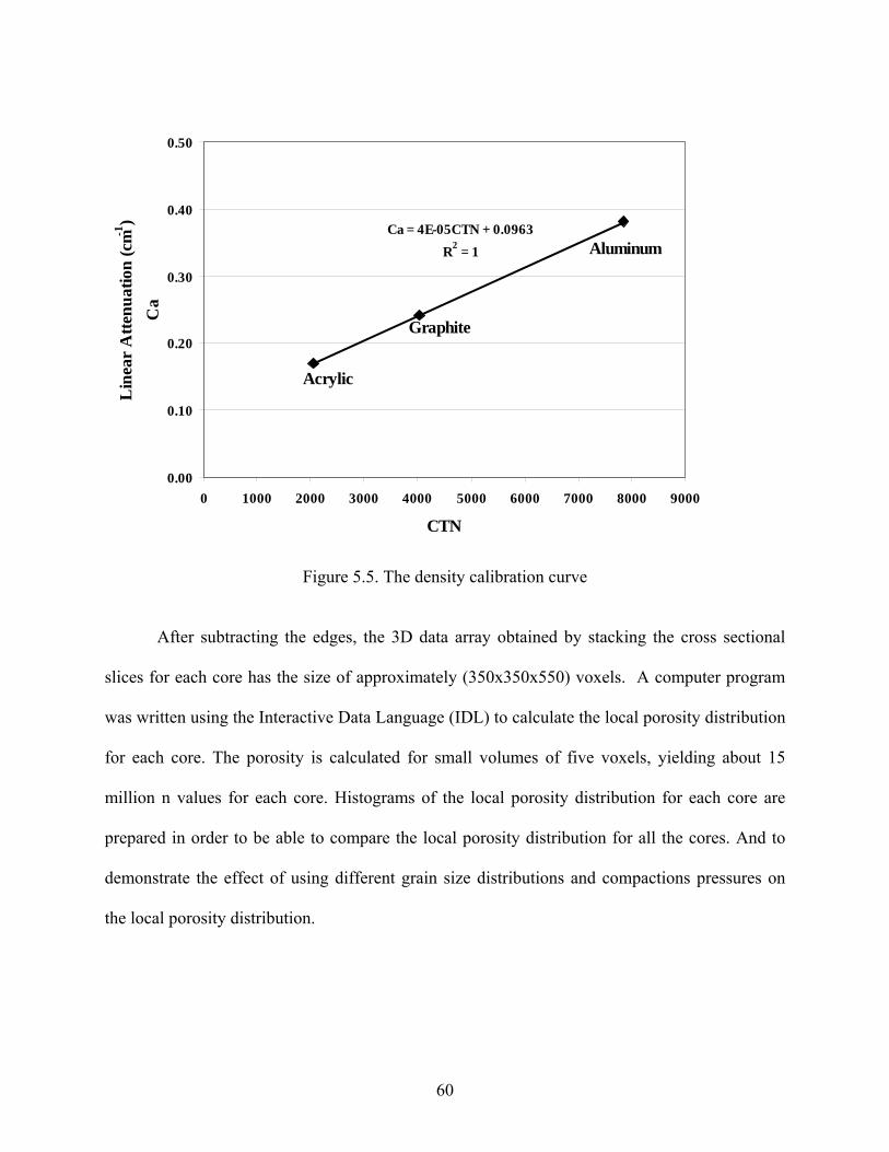
uter prog m

was written using the Interactive Data Language (IDL) to calculate the local porosity distribution

for each core. The porosity is calculated for small volumes of five voxels, yielding about 15

million n values for each core. Histograms of the local porosity distribution for each core are

prepared in order to be able to compare the local porosity distribution for all the cores. And to

demonstrate the effect of u compactions pressures on

the local porosity distribution.

0.50

Ca = 4E-05CTR

N + 0.2 = 1

0.00

0.10

0.20

0.40

0 1000 2000 3000 4000 5000 6000 7000 8000 9000

CTN

Lin

ear

Atte

nuat

ion

(cm-1

)

phite

Acrylic

luminum0963

A0.30

Ca

Gra

Figure 5.5. The density calibration curve

After subtracting the edges, the 3D data array obtained by stacking the cross sectional

slices for each core has the size of approximately (350x350x550) voxels. A comp ra

sing different grain size distributions and

60

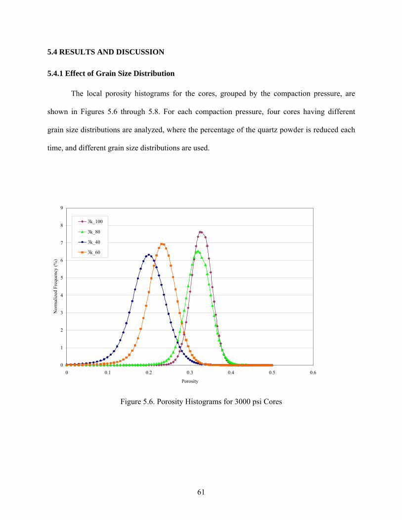
5.4 RESULTS AND DISCUSSION

5.4.1 Effect of Grain Size Distribution

The local porosity histograms for the cores, grouped by the compaction pressure, are

shown in Figures 5.6 through 5.8. For each compaction pressure, four cores having different

grain size distributions are analyzed, where the percentage of the quartz powder is reduced each

me, and different grain size distributions are used.

Figure 5.6. Porosity Histograms for 3000 psi Cores

ti

0

1

2

3

4

8

0 0.1 0.2 0.3 0.4 0.5 0.6

Porosity

Nor

mal

ized

eque

ncy

9

3k_100

3k_80

3k_40

3k_60

5

6

7

Fr

(%)

61

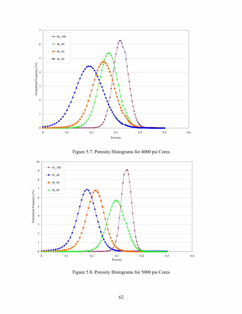
Figure 5.8. Porosity Histograms for 5000 psi Cores

Figure 5.7. Porosity Histograms for 4000 psi Cores

62

0

1

2

3

4

5

6

7

0 0.1 0.2 0.3 0.4 0.5 0.6

Porosity

Nor

mal

ized

Fre

quen

cy (%

) 4k_100

4k_80

4k_60

4k_40

0

1

2

3

4

5

6

7

8

9

10

0 0.1 0.2 0.3 0.4 0.5 0.6Porosit

Nor

mal

ized

Fre

quen

cy (%

)

5k_100

5k_40

5k_60

5k_80

y

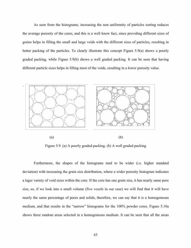
As seen from the histograms, increasing the non uniformity of particles sorting reduces

the average porosity of the cores, and this is a well know fact, since providing different sizes of

grains helps in filling the small and large voids ith the different sizes of particles, resulting in

better packing of the particles. To clearly illus re 5.9(a) shows a poorly

graded packing, while Figure 5.9(b) shows a well graded packing. It can be seen that having

different particle sizes helps in filling most of the voids, resulting in a lower porosity value.

.

Figure 5.9. (a) A poorly graded packing. (b) A well graded packing

eviation) with increasing the grain size distribution, where a wider porosity histogram indicates

lager variety of void sizes within the core. If the core has one grain size, it has nearly same pore

ze, so, if we look into a small volume (five voxels in our case) we will find that it will have

early the same percentage of pores and solids, therefore, we can say that it is a homogeneous

powder cores. Figure 5.10a

shows three ra t all the areas

w

trate this concept Figu

(a) (b)

Furthermore, the shapes of the histograms tend to be wider (i.e. higher standard

d

a

si

n

medium, and that results in the “narrow” histograms for the 100%

ndom areas selected in a homogeneous medium. It can be seen tha

63

contain nearly the same proportions of solid and void areas. On the other hand, looking at a core

having

(a) (b)

Figure 5.10. (a) Selection of a random area in a poorly graded specimen (b) selection of a

a variety of grain sizes, it will have different pore sizes, resulting from the different sizes

of the particles. Therefore, considering a small volume (5 voxels) in different positions, will

yield in a wide variety of void to solid ratios (Figure 5.10b), resulting in a high standard

deviation value and wider porosity histograms. A summary of the means and standard deviations

of the local porosity histograms is shown in Table 5.3.

random area in a well graded specimen.

Table 5.3: Summary of the statistical parameters for the porosity distributions Core Mean Std. Dev. Variance Skewness Kurtosis

3k_100 0.331951 0.0243841 0.0005946 -0.677971 9.15775 4k_100 0.324608 0.0307659 0.0009465 -0.742309 12.1766 5k_100 0.340829 0.0218543 0.0004776 0.387745 38.6906 3k_80 0.324644 0.031345 0.0009825 -1.16835 13.1452 4k_80 0.276654 0.0419643 0.001761 -0.67183 5.63001 5k_100 0.303162 0.0370358 0.0013717 -0.805755 5.93213 3k_60 0.237291 0.0385848 0.0014888 -1.47545 12.0596 4k_60 0.257841 0.0506909 0.0025696 -0.630058 5.4647 5k_60 0.220352 0.0413722 0.0017117 -1.286 10.4692

3k_40 06179 0.046165 0.0021312 -0.997361 7.97292 0.24k_40 0.20234 0.0628318 0.0039478 -0.630799 6.53747 5k_40 0.199239 0.0426337 0.0018176 -1.38796 10.8378

64

5.4.2 Effe

res are into s. Th each e the ain size

distribu ut ea was at a different comp essur porosity

histogra the fo s are shown in Figure ough 5

Figure 5.11. Porosity Histograms for 100% Quartz Powder Cores

ct of Compaction Pressure

The co grouped four group e cores in group hav same gr

tion, b ch core prepared action pr e. The

ms for ur group s 5.11 thr .14.

0

1

2

3

4

7

9

10

0 0.1 0.2 0.3 0.4 0.5 0.6Porosity

Nor

mal

izq

(%)

3k_100

4k_100

8 5k_100

5

6

ed F

reue

ncy

65

0

1

2

3

4

5

6

7

Nor

mal

ized

Fre

quen

cy (%

) .

3k_80

4k_80

5k_80

0 0.1 0.2 0.3 0.4 0.5 0.6Porosity

Figure 5.12. Porosity Histograms for 80% Quartz Powder Cores

Figure 5.13. Porosity Histogram for 60% Quartz Powder Cores

0

1

2

3

4

5

6

7

8

0 0.6

Nor

mal

ized

Fre

quen

cy (%

)

4k_60

5k_60

3k_60

0.1 0.2 0.3 0.4 0.5Porosity

s

66

from

histogram

the particles

particles` sh

are more suscep cores having a

0

1

2

3

4

5

6

7

8

0 0.1 0.2 0.3 0.4 0.5 0.6Porosity

Nor

mal

ized

Fre

quen

cy (%

) 4k_40

5k_40

3k_40

Figure 5.14. Porosity Histograms for 40% Quartz Powder Cores

It is expected that increasing the compaction pressure, should decrease the porosity of the

cores. This was not the case for the cores under investigation. Increasing the compaction pressure

3000 psi to 4000 psi resulted in decreasing the porosity as expected. But on the other hand,

increasing the compaction pressure to 5000 psi did not reduce the porosity. The porosity

s for the 5000 psi cores were located and different location each time with respect to

the 3000 and 4000 psi cores histograms (Figures 5.11 – 5.14). This may be due to the crushing of

that occurred at the very high pressure that resulted in the irregularity of the

apes, resulting in the unexpected values for the porosity. Moreover, large particles

tible to crushing than smaller ones, and it can be seen in the

67

higher percentage of large particles (40% and 6 Quartz powder) experience an irregularity of

results

5.4.3 Vertical Profiles of Porosity

0%

that can be justified by the crushing of the large (0.177 - 0.210 mm) particles at lower

compaction pressures of 4000 or even 3000 psi. It can also be realized that the porosity values

for the cores having the same grain size distribution, and different consolidation pressures are

very close to each other, because the lowest consolidation pressure used (3000 psi) is already a

very high pressure, and it might be enough to achieve the highest possible compaction for the

particles, and not much more compaction can be achieved by increasing the consolidation

pressure. As a result of the closeness of the porosity values for these cores, any imperfections in

the preparation process or the measurement could result in misleading trends in the results. This

could be another reason for the irregularity of the results for those cores.

To demonstrate the variation of porosity along the height of the cores, the average

porosity values for each slice were calculated for every core, and plotted against the distance

from the bottom of the core (Figure 15.15). All the profiles followed the same trend, where the

porosity increases near the ends, and decreases near the middle of the cores, this could be due the

boundary conditions of the cores where the edges doesn’t get as compacted as the middle part of

the cores.

68

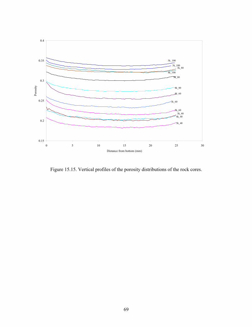
0.15

0.2

0.25

0.35

0 5 10 15 20 25 30

Distance from bottom (mm)

Po

5k_100

4k_100

4k_80

4k_60

3k_60

5k_60

4k_403k_40

5k_40

0.3

0.4

rosi

ty

3k_1003k_80

5k_80

Figure 15.15. Vertical profiles of the porosity distributions of the rock cores.

69

CHAPTER SIX

CONCLUSIONS AND RECOMMENDATIONS

.1 CONCLUSIONS

This thesis has two objectives. The first is to use micro-focus computed tomography (µCT)

study the shearing of granular materials, and the second is to characterize the variation of the

cal porosity distributions of synthetic rock cores with changing the grain size distribution and

onsolidation pressure using µCT. To achieve the first objective a triaxial specimen was scanned

t different strain levels to track the translation and rotation of the particles within the specimen.

he obtained values for translation and rotation were used to calculate the local strain

istribution within the specimen, and the distributions were compared to study the behavior of

the particles at different stages. To ach tive, twelve different rock cores were

scanned. The cor e different grain

ze distributions. Density calibration was performed to correlate the CT numbers to the bulk

Local porosity distributions of the cores were obtained using this

orr

particles in the triaxial specimen were obtained at a high degree of precision, for all stages of the

compression. This data was used to calculate the local strain distribution of the specimen

throughout the test. The calculated local strains were increasing throughout the experiment,

especially in the last stage, were a large increase in the local strains values was noticed. It was

also realized the local strains in the radial directions (ε and ε ) showed a similarity throughout

6

to

lo

c

a

T

d

ieve the second objec

es were prepared at different compaction pressures, and hav

si

density and porosity.

c elation. They were porosity compared to find the effect of compaction pressure and grain

size distribution.

Using the 3D volumetric data obtained by CT, the values of translation and rotation of the

x y

70

the test, where all the histograms took the shape of a Log-Normal distribution, with a greater

number of positive (extension) values then negative (contraction) values. This is due to the

axisymmetric conditions of the test. All the local shear strain histograms took the shape of a

logistic distribution; their values in the first two stages of the experiment lied in the narrow range

of ± 10% to 15%. On the last stage of compression a large increase in the shear strains values

in

in ly graded grains, higher porosity values and homogeneous pore

size

r

creased to reach up to ± 40%.

A similar trend was noticed in the rotation strain values, where all the histograms had the

shape of a logistic distribution. During the first and second stages of compression the rotation

strain values had values within ± 20%. They increased to reach about ±50% during the final

stage. A wide range of values was noticed for the dilatancy angles. At the beginning of the test,

the values where nearly evenly distributed between positive (dilatancy) and negative

(contraction). At the later stages, more positive values where obtained due to the dilative nature

of the specimen, until the last stage of the experiment where the positive values where dominant.

On the other hand, µCT showed an excellent ability to track the changes in the local porosity

distribution, and the homogeneity of pore sizes of the of the synthetic rock cores. It was found

that when using well graded grains less porosity values and inhomogeneous pore sizes were

obtained, while when us g poor

s were obtained, this was obtained from the mean and standard deviations of the porosity

distributions of the cores. No clear trend was obtained when increasing the consolidation

pressure. This could be due to the crushing of the particles at the ve y high consolidation

pressures, and some imperfections in the preparation process of the rock cores, which resulted in

inconsistent results for the porosity distribution.

71

6.2 RECOMMENDATIONS

• The data presented in the first part of this thesis could be compared with the values

obtained from different theoretical models. This could help in improving modeling of the

constitutive behavior of granular materials.

• In this study, plastic beads where used to model the behavior of granular materials. The

possibility of using other materials, like sand, should be investigated. This requires the

improvement of the CT scanner resolution, and the development of computer programs to

identify the particles and track their translation and rotation.

• In order to be able to relate the local values of strains and dilatancy angles to the global

values, the whole specimen should be scanned. This will require a larger scanning times,

and data sizes. It will also require very high computer capabilities and storage space. So,

in order to achieve this goal all these requirements should be considered.

in the preparation process, to reduce the

• Further studies should be conducted on the effect of increasing the consolidation pressure

on the porosity distribution of rock cores. A wider range of consolidation pressures

should be considered, with special care taken

amount of error caused my imperfections in the preparation of the cores.

72

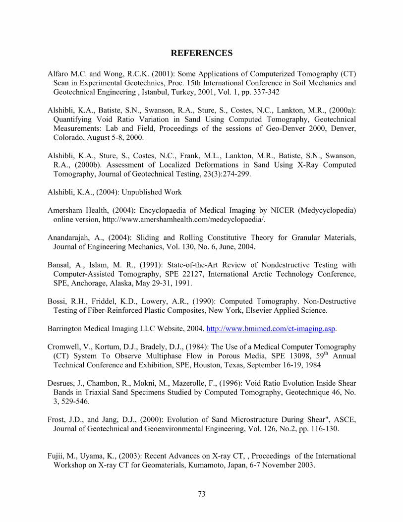
REFERENCES

M.C. and Wong, R.C.K. (2001): Some Applications of Computerized Tomography (CT) ental Geotechnics, Proc. 15th International Conference in Soil Mechanics and

chnical Engineering , Istanbul, Turkey, 2001, Vol. 1, pp. 337-342

i, K.A., Batiste, S.N., Swanson, R.A., Sture, S., Costes, N.C., Lankton,

Alfaro

Scan in ExperimGeote

Alshibl M.R., (2000a):

Quantifying Void Ratio Variation in Sand Using Computed Tomography, Geotechnical Measurements: Lab and Field, Proceedings of the sessions of Geo-Denver 2000, Denver, Colorado, August 5-8, 2000.

Alshibli, K.A., Sture, S., Costes, N.C., Frank, M.L., Lankton, M.R., Batiste, S.N., Swanson,

R.A., (2000b). Assessment of Localized Deformations in Sand Using X-Ray Computed Tomography, Journal of Geotechnical Testing, 23(3):274-299.

Alshibli, K.A., (2004): Unpublished Work

mersham Health, (2004): Encyclopaedia of Medical Imaging by NICER (Medycyclopedia) online version, http://www.amershamhealth.com/medcyclopaedia/.

Anandarajah, A., (2004): Sliding and Rolling Constitutive Theory for Granular Materials, Journal of Engineering Mechanics, Vol. 130, No. 6, June, 2004.

B

A

Bansal, A., Islam, M. R., (1991): State-of-the-Art Review of Nondestructive Testing with

Computer-Assisted Tomography, SPE 22127, International Arctic Technology Conference, SPE, Anchorage, Alaska, May 29-31, 1991.

Bossi, R.H., Friddel, K.D., Lowery, A.R., (1990): Computed Tomography. Non-Destructive

Testing of Fiber-Reinforced Plastic Composites, New York, Elsevier Applied Science.

arrington Medical Imaging LLC Website, 2004, http://www.bmimed.com/ct-imaging.asp. Cromwell, V., Kortum, D.J., Bradely, D.J., (1984): The Use of a Medical Computer Tomography

(CT) System To Observe Multiphase Flow in Porous Media, SPE 13098, 59th Annual Technical Conference and Exhibition, SPE, Houston, Texas, September 16-19, 1984

Desrues, J., Chambon, R., Mokni, M., Maz

Bands in Triaxial Sand Specimens Studieerolle, F., (1996): Void Ratio Evolution Inside Shear d by Computed Tomography, Geotechnique 46, No.

re During Shear", ASCE,

ujii, M., Uyama, K., (2003): Recent Advances on X-ray CT, , Proceedings of the International Workshop on X-ray CT for Geomaterials, Kumamoto, Japan, 6-7 November 2003.

3, 529-546.

rost, J.D., and Jang, D.J., (2000): Evolution of Sand MicrostructuFJournal of Geotechnical and Geoenvironmental Engineering, Vol. 126, No.2, pp. 116-130.

F

73

Honarpour, M.M., Cromwell, V., Hatton, D., Satchwell, R., Reservoir Rock (1985): Descriptions

Using Computed Tomography (CT), SPE 14272, 60th Technical Conference and Exhibition,

and Mass Energy-Absorption Coefficients”, NIST web site

SPE, Las Vegas, Nevada, September, 22-25, 1985.

Hubbell, J.H., and Seltzer, S.M., (1996): Tables of X-Ray Mass Attenuation Coefficients

(http://physics.nist.gov/PhysRefData/XrayMassCoef/cover.html).

. Kanatani (1979): A micropolar continuum theory for the flow of granular K materials,

International Journal of Engineering Science, Vol. 17, No. 4 (1979), pp. 419-432

Kmographic imagery: Application to the Geosciences, Computer & Geosciences,

27:381-400.

K he American Society for Nondestructive Testing (ASNT). http://www.asnt.org/publications/materialseval/basics/may00basics/may00basics.htm

K

uhn, M. R., Bagi, K., (2002): Particle Rotations in Granular Materials. 15th ASCE Engineering

M ournal of Physics Education 36, 442-451.

ukunoki, T., Otani, J., Obara, Y., Kaneko, K., (2003): Artifacts of X-ray CT Data in the

3.

da, M., Iwashita, K., (edt.), (1999): Introduction to Mechanics of Granular Materials, Balkima,

da, M., Konishi, J., and Nemat-Nasser, S. (1982): Experimental micromechanical evaluation of

O ita, K., Kakiuchi, T., (1997): Importance of Particle Rotation in Mechanics of

Granular Materials, Powders & Grains 97, Behringer & Jenkins (edt.), Balkema, pp. 207-210,

O hod for

Characterization of Failure in Soils, Soils and Foundations, Vol. 40, No. 2, 111-118.

etcham, A.R., Carlson, D.W., (2001): Acquisition, and optimization and interpretation of X-ray computed to

ropas-Hughes C., Neel, S., (2000): Basics of Computed Tomography. Website of T

TH Royal institute of technology (2001): Computed Tomography, November 2001.

K

Mechanics Conference, June 2 – 5, 2002, Columbia University, New York, NY.

ichael, G., (2001): X-ray Computed Tomography, J M

Analysis of Geomaterial Properties, Proceedings of the International Workshop on X-ray CT for Geomaterials, Kumamoto, Japan, 6-7 November 200

O

1999.

Ostrength of granular materials: Effects of particle rolling. Mech. of Materials, 1(4), 269–283.

da, M., Iwash

(1997).

tani, J., Mukunoki, T., Obara, Y., (2000): Application of X-Ray CT Met

74

Rowe, P.W., (1962): The Stress Dilatancy Relation for Static Equilibrium of an Assembly of

heats, M.J., (2000): Advanced Data Processing for Volumetric Computed Tomography Data, A

trumas, N., Antonyshyn, O., Yaffe, M. J., Mawdsley, G., Cooper, P., (1995): Computed

g of the Canadian Society of Plastic Surgeons, Saskatoon, Saskatchewan, June 1995.

drs), “Applications of X-ray Computed

Flow Visualization. 62nd Annual Technical Conference and Exhibition of the Society of

W

Yoshikawa, H., (2004): X-ray Computed Tomography. Website of Inouye Labs, Japan.

http://ctlab.bk.tsukuba.ac.jp/~hiroki/blind/x-rayCT.html

Particles in Contact. Proceedings of the Royal Society. Vol. 269, Series A, pp 500-527.

SMasters Thesis, University of California Davis.

Steude, J.S., and F. Hopkins. (1994): Industrial X-ray computed tomography applied to soil

research. Tomography of soil-water-root processes. SSSA Spec. Publ. 36. SSSA, Madison, WI.

STomography Artifacts: An Experimental Investigation of Causative Factors, 49th Annual Meetin

Tatsuoka, F. (1987): Discussion: The Strength and Dilatancy of Sands. Geotechnique, 37(2),

219-226.

Van Geet, M., Lagrou, D., and Swennen, R. (2003): Porosity Measurements of Sedimentary Rocks by Means of Microfocus X-ray Computed Tomography (µCT),” from Mees, F. Swennen, R., Van Geet, M. & Jacobs, P. (eTomography in the Geosciences”, Geological Society of London, Special Publication, Vol. 215, pp. 51-60.

Vardoulakis, I., Sulem, J., (1995), Bifurcation Analysis in Geomechanics, Blackie Academic &

Professional, Bishopbriggs, Glasgow, 1995. Wang, L.B., Frost, J.D., and Lai, J.S., (1999): Non-Invasive Measurement of Permanent Strain

Field Resulting from Rutting in Asphalt Concrete, Transportation Research Record, No. 1687, pp. 85-94.

Washington State University (2004). X-Ray Computed Tomography Facility WAX-CT

(http://www.waxct.wsu.edu/) Wevers, M., De Meester, P., Swennen, R., (2000): Microfocus X-ray Computer Tomography in

Materials Research, Proceeding of the 15th World Conference on Nondesructive Testing, Roma, Italy, 15-21 October 2000.

Withjack, E. M., (1987): Computed Tomography for Rock-Property Determination and Fluid-

Petroleum Engineers, Dallas, TX, September, 1987.

ood, D.M. (1990): Soil Behavior and Critical State Soil Mechanics, Cambridge, Cambridge University Press.

75

APPENDIX A: TRANSLATION AND ROTATION HISTOGRAMS

Figure A1: Normalized Translation Histograms at εz = -13.7 % (Normalization Value = 6.6 mm)

0 10 20 30

60

40eq

uenc

y (P

0

20Fr

Normalized Translation (%), X Direction

artic

les)

0 10 20 300

20

60

40

Normalized Translation (%), Y Direction

Frar

ticle

s)eq

uenc

y (P

0 10 20 3 40 500

20

40

0Normalized Translation (%), Z Direction

Freq

uenc

y (P

artic

les)

76

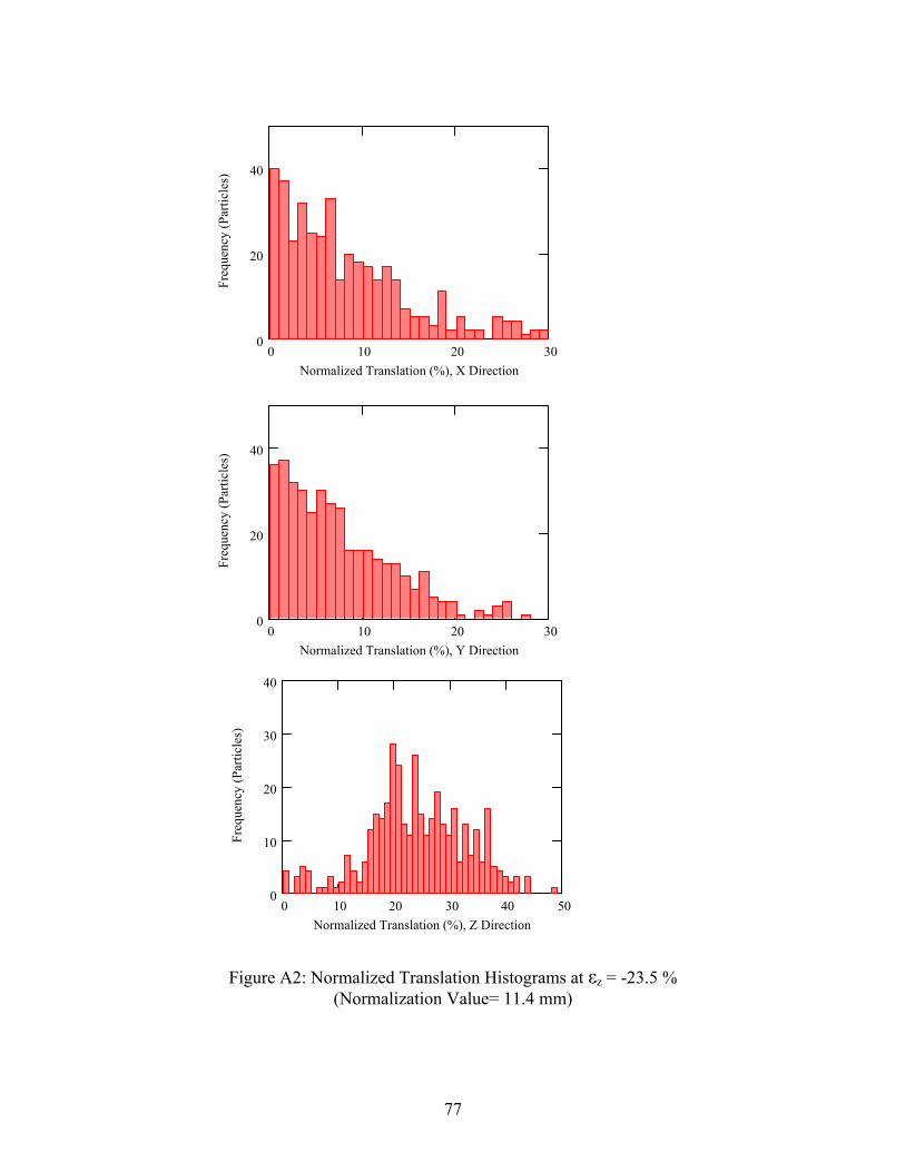
Figure A2: Normalized Translation Histograms at εz = -23.5 % (Normalization Value= 11.4 mm)

0 10 2 00

20

40

0 3Normalized Translation (%), Y Direction

Freq

uenc

y (P

artic

les)

0 10 20 30 40 500

10

20

30

40

Normalized Translation (%), Z Direction

Freq

uenc

y (P

artic

les)

0 10 2 00

20

40

0 3Normalized Translation (%), X Direction

Freq

uenc

y (P

artic

les)

77

APPENDIX B: LOCAL STRAIN HISTOGRAMS

78

Figure B1: Local strains histograms at εz = -13.7%

εxz0.4 0.2 0.2 0.4

0

20

40

Freq

uenc

y (P

artic

les)

εx0.4 0.2 0 0.2 0.4

0

30

40

20

10

Freq

uenc

y (P

artic

les)

εy0.4 0.2 0 0.2 0.4

0

10

20

30

40

Freq

uenc

y (P

artic

les)

εz0.4 0.2 0 0.2 0.4

0

20

60

0

40

Freq

uenc

y (P

artic

les)

εyz0.4 0.2 0.2 0.4

40

00

20

Freq

uenc

y (P

artic

les)

0.4 0.2 0 0.20

0.4

40

20

Frat

icle

s)eq

uenc

y (P

εxy

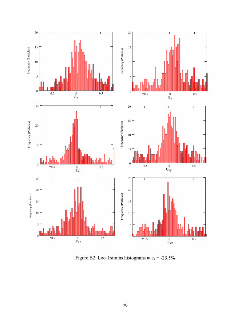
Figure B2: Local strains histograms at εz = -23.5%

= -23.5%

εxy0.5 0 0.5

0

15

20

10

5

Freq

uenc

y (P

artic

les)

εx0.5 0 0.5

0

5

10

15

20Fr

eque

ncy

(Par

ticle

s)

εy0.5 0 0.5

0

5

10

15

20

Freq

uenc

y (P

artic

les)

εz0.5 0 0.5

0

10

20

30

Freq

uenc

y (P

artic

les)

εyz0.5 0 0.5

0

5

10

15

20

25

Freq

uenc

y (P

artic

les)

εxz0.5 0 0.5

0

5

10

15

20

25

Freq

uenc

y (P

artic

les)

γxz

79

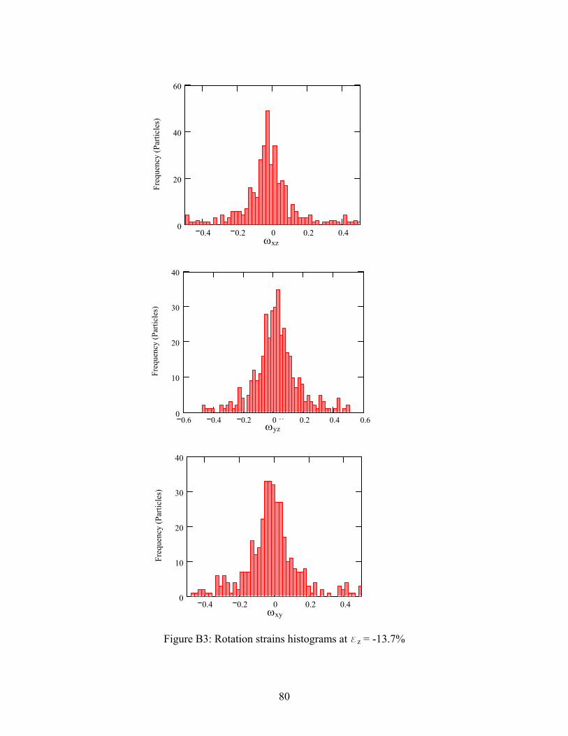
Figure B3: Rotation strains histograms at ez = -13.7%

ωxz

0.4 0.2 0 0.2 0.40

10

20

30

40

Freq

uenc

y (P

artic

les)

ωxy

0.4 0.2 0 0.2 0.40

20

40

60

Freq

uenc

y (P

artic

les)

ω xz

0.6 0.4 0.2 0 0.2 0.4 0.60

10

20

30

40

Freq

uenc

y (P

artic

les)

ωyzωyz

ωxy

80

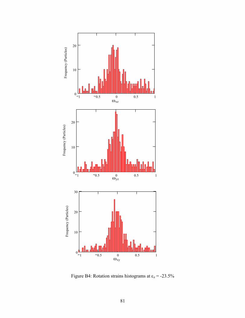
ωx

z1 0.5 0 0.5 10

10

20

Freq

uenc

y (P

artic

les)

ωxz

1 0.5 0 0.5 10

10

20

Freq

uenc

y (P

artic

les)

ωy

Figure B4: Rotation strains histograms at εz = -23.5%

zωyz

1 0.5 0 0.5 10

10

20

30

Freq

uenc

y (P

artic

les)

ωx

yωxy

81

VITA Bashar Alramahi was born on September 7th, 1979, in Beirut, Lebanon. He studied high school at

Al-Ittihad School in Amman, Jordan, and graduated in 1997. He received his bachelor’s degree

in civil engineering from Birzeit University, Ra allah, Palestine, in August, 2002. He came to

the United States in January, 2003 to pursue a master’s degree in geotechnical engineering at

Louisiana State University, Baton Rouge, Louisiana. It is anticipated that he will fulfill the

requirements for the master’s degree in civil engineering in August, 2004.

m

82