Embed Size (px)
Citation preview
A part of BMT in Energy and Environment
Final Report
R.N1609.001.00.doc
June 2010
Assessment of Salinity Responseto River Flow Modification in theHunter River Estuary
K:\N1609_HUNTER_RIVER_ESTUARY_SALINITY_MODELLING\DOCS\R.N1609.001.00.DOC
Assessment of Salinity Response to River Flow
Modification in the Hunter River Estuary
Prepared For: NSW Office of Water
Prepared By: BMT WBM Pty Ltd (Member of the BMT group of companies)
Offices
BrisbaneDenver
KarrathaMelbourne
MorwellNewcastle
PerthSydney
Vancouver
K:\N1609_HUNTER_RIVER_ESTUARY_SALINITY_MODELLING\DOCS\R.N1609.001.00.DOC
DOCUMENT CONTROL SHEET
BMT WBM Pty LtdBMT WBM Pty Ltd126 Belford StreetBROADMEADOW NSW 2292AustraliaPO Box 266Broadmeadow NSW 2292
Tel: +61 2 4940 8882Fax: +61 2 4940 8887
ABN 54 010 830 421 003
www.wbmpl.com.au
Document :
Project Manager :
R.N1609.001.00.doc
Luke Kidd
Client :
Client Contact:
Client Reference
NSW Office of Water
Graham Carter
Title : Assessment of Salinity Response to River Flow Modification in the Hunter River Estuary
Author : Luke Kidd
Synopsis : This report summarises development and calibration of a numerical hydrodynamic model (TUFLOW-FV) to assess the response of salinity within the Hunter River Estuaryto flow changes from the Hunter River, Paterson River and Williams River.
REVISION/CHECKING HISTORY
REVISION
NUMBER
DATE OF ISSUE CHECKED BY ISSUED BY
0 9/06/2010 LJK LJK
DISTRIBUTION
DESTINATION REVISION
0 1 2 3
NoW
BMT WBM File
BMT WBM Library
1-e
1-e
1
CONTENTS I
K:\N1609_HUNTER_RIVER_ESTUARY_SALINITY_MODELLING\DOCS\R.N1609.001.00.DOC
CONTENTS
Contents i
List of Figures ii
List of Tables iii
1 INTRODUCTION 1
1.1 The Project 1
1.2 Modelling Scope 1
1.3 Report Outline 2
2 STUDY AREA DESCRIPTION 3
2.1 Overview 3
2.2 Other Background Information 3
3 HYDRODYNAMIC MODEL DEVELOPMENT AND CALIBRATION 6
3.1 Overview 6
3.2 The Finite Volume Model 6
3.3 TUFLOW-FV Model Description 7
3.4 TUFLOW-FV Model Development 7
3.4.1 Model extents 7
3.4.2 Bathymetry 7
3.4.3 Model geometry 8
3.4.4 Boundary conditions 9
3.5 WaterCAST Model Development 9
3.5.1 Model description 9
3.5.2 Catchment delineation and model extents 9
3.5.3 Selection of inflow locations 10
3.5.4 Landuse mapping 10
3.5.5 Rainfall-runoff model 14
3.5.6 Distribution of runoff volumes 16
3.6 TULOW-FV Model Calibration 16
3.6.1 Boundary conditions 16
3.6.1.1 Water level 16
LIST OF FIGURES II
K:\N1609_HUNTER_RIVER_ESTUARY_SALINITY_MODELLING\DOCS\R.N1609.001.00.DOC
3.6.1.2 Salinity 18
3.6.2 Results 18
3.6.2.1 Water levels 18
3.6.2.2 Salinity 19
4 SCENARIO MODELLING 23
4.1 Overview 23
4.2 Integrated Quantity and Quality Modelling (IQQM) 23
4.3 Boundary Conditions 24
4.3.1 Hydrodynamics 24
4.3.2 Salinity 25
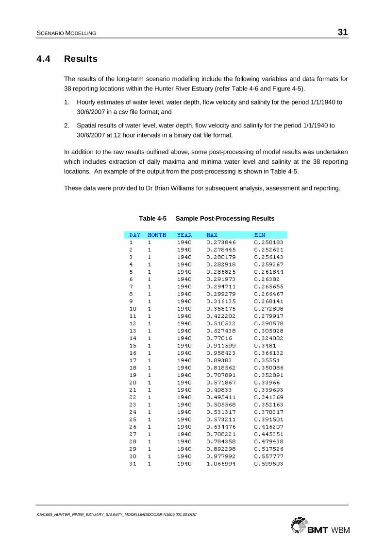
4.4 Results 31
5 CONCLUSIONS AND RECOMMENDATIONS 34
6 REFERENCES 36
APPENDIX A: TUFLOW-FV MODEL DESCRIPTION A-1
APPENDIX B: NOW APPROVAL LETTER B-1
APPENDIX C: SALINITY CALIBRATION LETTER 1 C-1
APPENDIX D: SALINITY CALIBRATION LETTER 2 D-1
APPENDIX E: NOW REQUEST FOR ADDITIONAL INFORMATION E-1
APPENDIX F: MEMORANDUM OF ADDITIONAL INFORMATION F-1
LIST OF FIGURES
Figure 2-1 Study Area, Hunter River Estuary 5
Figure 3-1 Model Geometry and Extents 11
Figure 3-2 WaterCAST Catchment Model Extents 12
Figure 3-3 Landuse Mapping for WaterCAST model 13
Figure 3-4 Calibrated Runoff Depths (modelled versus observed) 15
LIST OF TABLES III
K:\N1609_HUNTER_RIVER_ESTUARY_SALINITY_MODELLING\DOCS\R.N1609.001.00.DOC
Figure 3-5 Tidal Water Level Data 17
Figure 3-6 River Flow Data 17
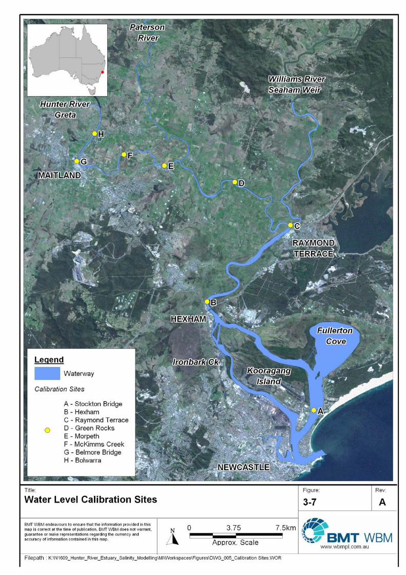
Figure 3-7 Water Level Calibration Sites 20
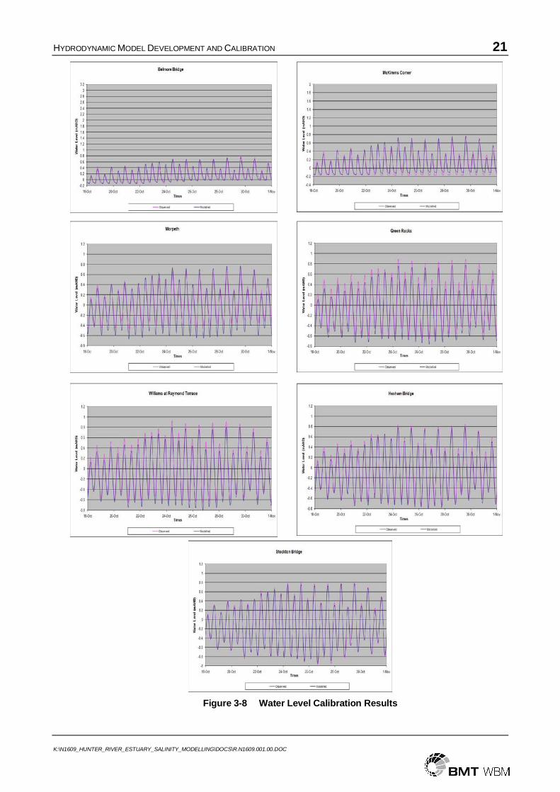
Figure 3-8 Water Level Calibration Results 21
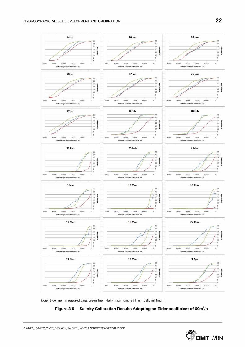
Figure 3-9 Salinity Calibration Results Adopting an Elder coefficient of 60m2/s 22
Figure 4-1 Flow Versus EC at Glen Martin 27
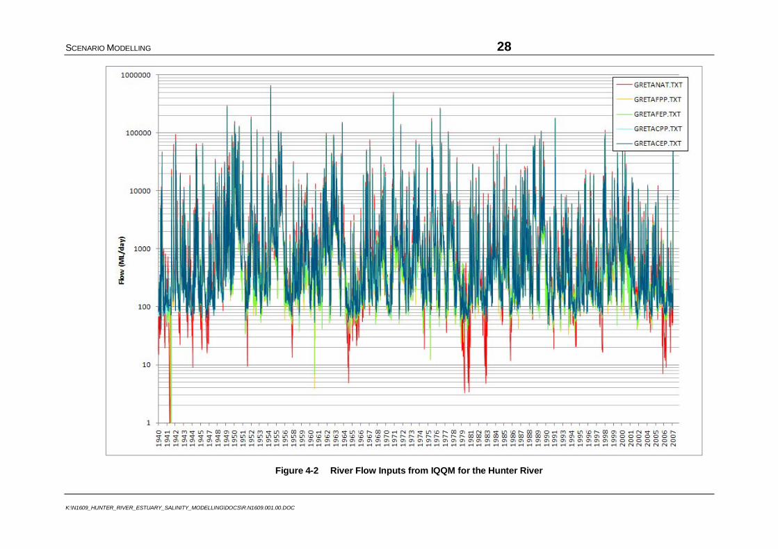
Figure 4-2 River Flow Inputs from IQQM for the Hunter River 28
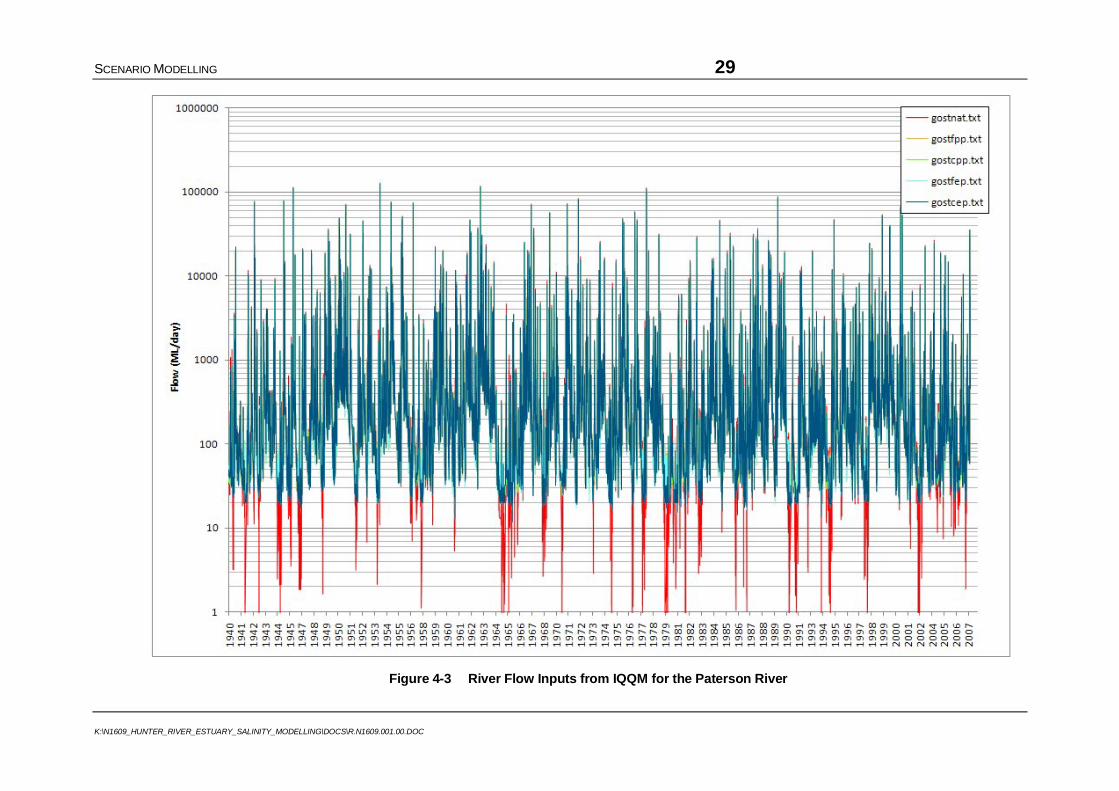
Figure 4-3 River Flow Inputs from IQQM for the Paterson River 29
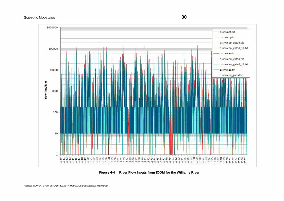
Figure 4-4 River Flow Inputs from IQQM for the Williams River 30
Figure 4-5 Reporting Locations 33
LIST OF TABLES
Table 3-1 Adopted SIMHYD Rainfall-Runoff Parameters 15
Table 3-2 Summary of Predicted Salinity Gradients 19
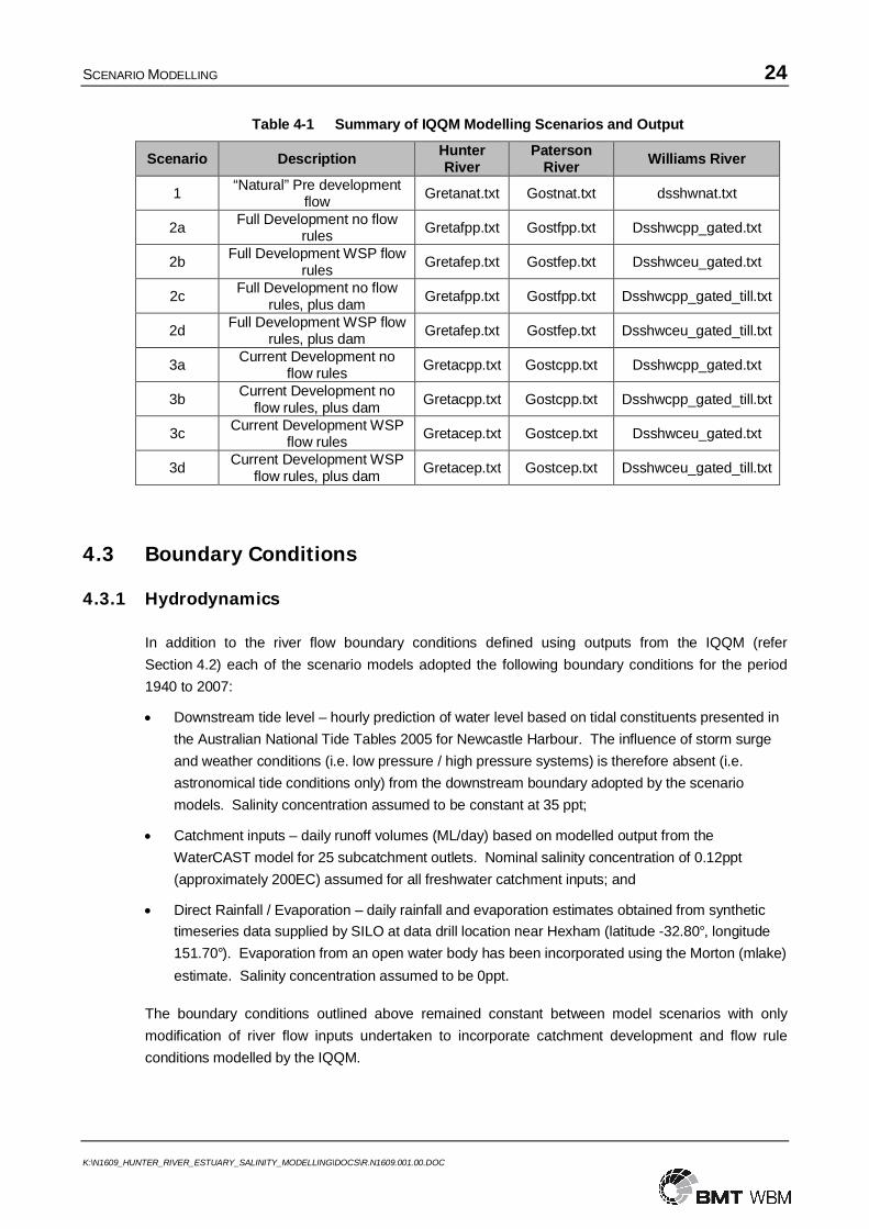
Table 4-1 Summary of IQQM Modelling Scenarios and Output 24
Table 4-2 Assumed Flow and EC Relationship for the Hunter River (Greta) 25
Table 4-3 Summary of Flow and Salinity for the Paterson River (Gostwyck) 26
Table 4-4 Flow and Salinity Summary for the Williams River 26
Table 4-5 Sample Post-Processing Results 31
Table 4-6 Coordinates of Reporting Locations 32
INTRODUCTION 1
K:\N1609_HUNTER_RIVER_ESTUARY_SALINITY_MODELLING\DOCS\R.N1609.001.00.DOC
1 INTRODUCTION
This report has been prepared by BMT WBM for the NSW Office of Water (NoW) (formerly the
Department of Water and Energy) to assist with an assessment of salinity response to river flow
modification within the Hunter River Estuary.
1.1 The Project
Salinity conditions within the Hunter River Estuary, particularly tidal pool areas upstream of Hinton,
may vary considerably in response to the volume of freshwater from upstream major rivers (e.g.
Hunter River and Paterson River), local catchment runoff, long-term climatic conditions and variation
of downstream tidal conditions at the entrance of the estuary (e.g. diurnal water level variations, neap
and spring cycles etc).
This project seeks to provide further insight into salinity changes within the Hunter River Estuary
obtained from previous one-dimensional hydrodynamic modelling undertaken on behalf of the NOW
by Sanderson, Redden and Smith (2002), Sanderson (2005) and Sanderson (2007). The nature of
this work included an assessment of changes in salinity of the Hunter River in response to modified
river flow, and subsequent investigations which incorporated seasonal and climatic changes that
were not considered by the previous study. The current investigation of hydrodynamics and salinity
within the Hunter River Estuary was undertaken as part of the Water Sharing Plan investigations
carried out by the NoW.
River flow modification scenarios have been simulated using a two-dimensional hydrodynamic model
(TUFLOW-FV) coupled with outputs from the Integrated Quantity Quality Model (IQQM) of the Hunter
River catchment. IQQM outputs were adopted by the TUFLOW-FV model to provide an estimate of
the response of salinity within the Hunter River Estuary as a consequence of river flow changes at
Greta, Gostwyck and Seaham Weir. The modelling provides a basis for an assessment of the
general effect on salinity conditions as a consequence of river flow modifications predicted over a
period of some 67 years.
1.2 Modelling Scope
Adoption of TUFLOW-FV for this study has enabled an assessment of long-term salinity response to
river flow modification in the Williams River, Paterson River and Hunter River catchments. An
estimate of resultant salinity concentrations at key points of interest in response to rainfall /
evaporation, river inflow, tidal variations and local catchment runoff has been obtained and compared
with other model scenarios to quantify characteristics of the tidal pool with respect to long term salinity
conditions under differing river flow conditions.
Sub-daily (e.g. hourly) predictions of hydrodynamics (i.e. water level, water depth and flow velocity)
and salinity for the nominated modelling period (1940 to 2007) were obtained using the TUFLOW-FV
model. The following sections outline the development, calibration and scenario modelling
undertaken by BMT WBM. Separate analysis and assessment of TUFLOW-FV model results is to be
undertaken by Dr Brian Williams.
INTRODUCTION 2
K:\N1609_HUNTER_RIVER_ESTUARY_SALINITY_MODELLING\DOCS\R.N1609.001.00.DOC
1.3 Report Outline
This report details the methodology used to develop and calibrate a two dimensional finite volume
model, and provides a summary of the modelling assumptions adopted to assess salinity response to
river flow modification within the Hunter River, Paterson River and Williams River. Model scenarios
utilise outputs from the IQQM prepared by the NoW for the Hunter River Catchment.
Section 1 provides an introduction to the Project;
Section 2 provides a description of the study area;
Section 3 provides details relating to TUFLOW-FV model development and calibration;
Section 4 provides details relating to the long-term assessment of impacts on estuary characteristics
(hydrodynamics and salinity), for a range of river flow modification scenarios; and
Section 5 provides conclusions of the modelling tasks undertaken and recommendations of future
work;
Appendix A provides details of the numerical formulation and a description of the physics simulated
by the model;
Appendix B letter of acceptance provided by NoW to proceed with scenario modelling;
Appendix C salinity calibration letter provided by BMT WBM clarifying aspects of the salinity
calibration and justification for adoption of model parameters;
Appendix D salinity calibration letter provided by BMT WBM to further clarify selection of model
parameters;
Appendix E letter from NoW requesting additional information relating to model sensitivity; and
Appendix F memorandum provided by BMT WBM detailing sensitivity tests performed to address
questions raised by NoW.
STUDY AREA DESCRIPTION 3
K:\N1609_HUNTER_RIVER_ESTUARY_SALINITY_MODELLING\DOCS\R.N1609.001.00.DOC
2 STUDY AREA DESCRIPTION
2.1 Overview
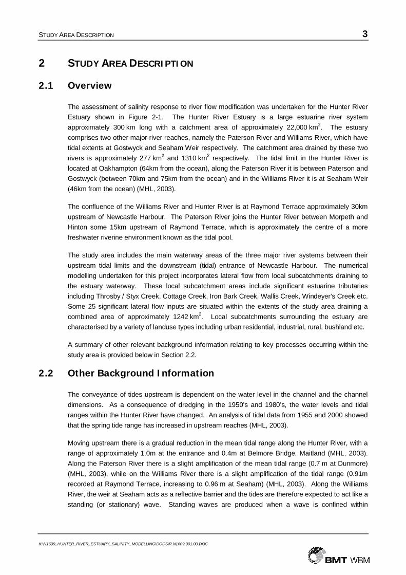
The assessment of salinity response to river flow modification was undertaken for the Hunter River
Estuary shown in Figure 2-1. The Hunter River Estuary is a large estuarine river system
approximately 300 km long with a catchment area of approximately 22,000 km2. The estuary
comprises two other major river reaches, namely the Paterson River and Williams River, which have
tidal extents at Gostwyck and Seaham Weir respectively. The catchment area drained by these two
rivers is approximately 277 km2 and 1310 km2 respectively. The tidal limit in the Hunter River is
located at Oakhampton (64km from the ocean), along the Paterson River it is between Paterson and
Gostwyck (between 70km and 75km from the ocean) and in the Williams River it is at Seaham Weir
(46km from the ocean) (MHL, 2003).
The confluence of the Williams River and Hunter River is at Raymond Terrace approximately 30km
upstream of Newcastle Harbour. The Paterson River joins the Hunter River between Morpeth and
Hinton some 15km upstream of Raymond Terrace, which is approximately the centre of a more
freshwater riverine environment known as the tidal pool.
The study area includes the main waterway areas of the three major river systems between their
upstream tidal limits and the downstream (tidal) entrance of Newcastle Harbour. The numerical
modelling undertaken for this project incorporates lateral flow from local subcatchments draining to
the estuary waterway. These local subcatchment areas include significant estuarine tributaries
including Throsby / Styx Creek, Cottage Creek, Iron Bark Creek, Wallis Creek, Windeyer’s Creek etc.
Some 25 significant lateral flow inputs are situated within the extents of the study area draining a
combined area of approximately 1242 km2. Local subcatchments surrounding the estuary are
characterised by a variety of landuse types including urban residential, industrial, rural, bushland etc.
A summary of other relevant background information relating to key processes occurring within the
study area is provided below in Section 2.2.
2.2 Other Background Information
The conveyance of tides upstream is dependent on the water level in the channel and the channel
dimensions. As a consequence of dredging in the 1950’s and 1980’s, the water levels and tidal
ranges within the Hunter River have changed. An analysis of tidal data from 1955 and 2000 showed
that the spring tide range has increased in upstream reaches (MHL, 2003).
Moving upstream there is a gradual reduction in the mean tidal range along the Hunter River, with a
range of approximately 1.0m at the entrance and 0.4m at Belmore Bridge, Maitland (MHL, 2003).
Along the Paterson River there is a slight amplification of the mean tidal range (0.7 m at Dunmore)
(MHL, 2003), while on the Williams River there is a slight amplification of the tidal range (0.91m
recorded at Raymond Terrace, increasing to 0.96 m at Seaham) (MHL, 2003). Along the Williams
River, the weir at Seaham acts as a reflective barrier and the tides are therefore expected to act like a
standing (or stationary) wave. Standing waves are produced when a wave is confined within
STUDY AREA DESCRIPTION 4
K:\N1609_HUNTER_RIVER_ESTUARY_SALINITY_MODELLING\DOCS\R.N1609.001.00.DOC
boundaries such as an upstream structure or control (e.g. weir). As a consequence the tides in the
Williams River are weaker (by a factor of 0.3), when compared to the Hunter River.
Tidal lags also vary within the three rivers. Along the Hunter River at Bolwarra the low tides lag 8.8 to
6.3 hrs after the entrance tide and the high lags 3.8 hrs. Along the Paterson River at the Paterson
Railway Bridge the low tides are 6.1 to 5.3 hrs after the entrance tide and the high tide lags by 4.3
hrs, and along the Williams River at Seaham Weir the low tides are 3.3 to 2.5 hrs after the entrance
tide and the high tide is 1.8 hrs after (MHL, 1995). In the lower estuary the tidal excursion is around
10km during spring tides (MHL, 1995).
Maximum tidal velocities decrease upstream with values of around 1.0 m/s near the entrance during
the ebb tide to around 0.5 m/s at Morpeth (48km upstream) (MHL, 2003). During the flood tide the
maximum velocities are similar, at around 0.9 m/s near the entrance.
Low frequency oscillations in tidal level of about 3 to 10 days period with amplitudes of 0.1m have
been recorded within the estuary (MHL, 2003).
Hydrodynamic modelling has previously been undertaken by BMT WBM to investigate the potential
for ocean exchange and flushing, by assessing e-folding flushing times. The e-folding time
corresponds to the time taken for average tidal conditions to reduce the concentration of a
conservative constituent inside the lower estuary from a value of 1.0 to a value of 0.368 (1/e) under
the forcing of clean ocean water (concentration of 0.0) and the physical processes of advection and
dispersion. Generally, areas close the ocean will have a very short flushing time (indicative of the
time it takes for water particles at these locations to be advected out of the estuary system), while
areas near the tidal limits of the estuary have long flushing times (and are much more influenced by
freshwater inflows to the estuary).
Results from previous hydrodynamic modelling indicate that the lower estuary is dominated by tidal
processes and has a very short flushing time, in the order of 1-5 days, suggesting that the daily tidal
motions are quite effective at flushing surface waters of the lower estuary. Moving further upstream
to Hexham the flushing time doubles to around 10 or 11 days.
HYDRODYNAMIC MODEL DEVELOPMENT AND CALIBRATION 6
K:\N1609_HUNTER_RIVER_ESTUARY_SALINITY_MODELLING\DOCS\R.N1609.001.00.DOC
3 HYDRODYNAMIC MODEL DEVELOPMENT AND CALIBRATION
3.1 Overview
As discussed, river flow modification scenarios have been simulated using a two-dimensional
hydrodynamic model coupled with outputs from the IQQM. The following sections provide details of
the selected model (TUFLOW-FV) including its development (i.e. extents, bathymetry data, geometry,
boundary conditions) and calibration to water level and salinity.
3.2 The Finite Volume Model
The Finite Volume Model (herein referred to as TUFLOW-FV) solves the conservative integral form of
the non-linear shallow water equations (NLSWE) (i.e. assuming that pressure varies hydrostatically
with depth), including viscous flux terms and source terms for Coriolis force, bottom-friction and
various surface and volume stresses. The scheme is also capable of simulating the advection and
dispersion of multiple scalar constituents (e.g. salinity, temperature) within the model domain.
The spatial domain (or study area extents) is discretised using contiguous, non-overlapping irregular
triangular and quadrilateral “cells”. Advantages of an irregular flexible mesh include:
The ability to smoothly resolve bathymetric features of varying spatial scales (e.g. dredged
channels adjacent to broad shoaled areas);
The ability to smoothly and flexibly resolve boundaries such as coastlines; and
The ability to adjust model resolution to suit the requirements of particular parts of the model
domain without resorting to a “nesting” approach.
The flexible mesh approach has significant benefits when applied to study areas involving complex
coastlines and embayments, varying bathymetries and sharply varying flow and scalar concentration
gradients. TUFLOW-FV presently accommodates a wide variety of boundary conditions, including
some of which are necessary for modelling the processes of importance to the present study, such
as:
Water level timeseries;
In/out flow timeseries;
Mean Sea Level Pressure gradients;
Wind stress; and
Wave radiation stress.
Bed friction is modelled using a Manning’s roughness formulation and Coriolis force is also included
in the model formulation. The model is currently fully operational as a 2-dimensional NLWSE solver,
and development work to extend the model to a 3-dimensional NLSWE solver including baroclinic
forcing is almost complete.
HYDRODYNAMIC MODEL DEVELOPMENT AND CALIBRATION 7
K:\N1609_HUNTER_RIVER_ESTUARY_SALINITY_MODELLING\DOCS\R.N1609.001.00.DOC
3.3 TUFLOW-FV Model Description
TUFLOW-FV is a hydrodynamic model which solves the non-linear shallow water equations
(NLSWE) on a flexible mesh containing triangular and quadrilateral cells. The model code has been
in development by BMT WBM for the past 3 years and has recently been successfully applied to a
number of different projects including:
Coral Sea and Queensland coastline hydrodynamic model;
Tropical cyclone generated storm tide modelling as part of the Cairns storm tide study;
Tsunami shoaling and run-up as part of a risk assessment for Lihir Gold mine expansion;
Hydrodynamics and salinity intrusion in the South Alligator River under existing and future
climate change scenarios as part of the NCVA climate change assessment for Kakadu National
Park; and
Saltwater dispersion modelling of the Coorong.
TUFLOW-FV leverages the parallel processing capabilities of modern computer workstations, using
implementation of shared memory parallelisation. As such, the model can be used to simulate 2-
dimensional hydrodynamics of a waterway system at timesteps of a few seconds over decadal
timescales (even up to 70 years). When linked with catchment models or long-term historical
estimates of river flow, TUFLOW-FV can be used to continuously simulate hydrodynamic and
advection / dispersion processes within a water body such as the Hunter River Estuary.
Details of the numerical formulation and a description of the physics simulated by the model are given
in Appendix A.
3.4 TUFLOW-FV Model Development
3.4.1 Model extents
The Hunter River Estuary is a large estuarine river system with three main tidal reaches, namely the
Hunter River, Paterson River and Williams River. The confluence of the Williams River and Hunter
River is at Raymond Terrace approximately 30 km upstream of Newcastle Harbour (i.e. Pacific
Ocean). The Paterson River joins the Hunter River between Morpeth and Hinton some 15 km
upstream of Raymond Terrace, which is the approximate geographical centre of the tidal pool area.
The tidal limit in the Hunter River is located at Oakhampton (64 km from the ocean), along the
Paterson River it is between Paterson and Gostwyck (between 70 km and 75 km from the ocean) and
in the Williams River it is at Seaham Weir (46 km from the ocean) (MHL, 2003).
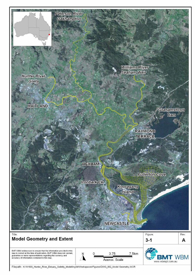
The TUFLOW-FV model incorporates the main estuarine waterways of the Hunter River, Paterson
River and Williams River to their tidal extents. A map of the model extents is shown in Figure 3-1.
3.4.2 Bathymetry
Bathymetric data are used to describe the topography of the waterway over the domain of a
numerical model system. A number of data sources have been utilised in the development of the
HYDRODYNAMIC MODEL DEVELOPMENT AND CALIBRATION 8
K:\N1609_HUNTER_RIVER_ESTUARY_SALINITY_MODELLING\DOCS\R.N1609.001.00.DOC
model bathymetry for the Hunter River system. Sources of data used in preparing a Digital Elevation
Model (DEM) for the Hunter River Estuary include:
Newcastle Port Corporation (NPC) – Hydro surveys of the lower estuary;
Department of Commerce (DoC) – River transects upstream from Green Rocks, extending along
the Paterson and the Hunter River. The data was sourced from hard copy transects, which were
manually entered and converted from Newcastle Sewerage datum;
Roads and Traffic Authority (RTA) – Hydro surveys between Heatherbrae to Raymond Terrace;
and
DECCW / Department of Natural Resources (DNR) – River transects along the Williams River
and Paterson Rivers.
The hydro survey data for the Paterson River extends approximately 4 km upstream from Woodville,
(~7.5km downstream from Paterson). An additional 15 km of river were required to extend the model
to the tidal limit along the Paterson tributary. The extension of the model over these last 15 km has
been approximated based on the thalweg depths of the river upstream to this point.
Hydro survey data exist along the full length of the tidal reach along the Williams River, to Seaham
Weir, with the Weir acting as an upstream boundary with limited inflow. A deep pool exists upstream
of Seaham Weir.
Along the Hunter River, hydro survey data exist from the mouth all the way up to Oakhampton. A
further ~2 km of river was required to extend the model to the tidal limit along the Hunter River and
was estimated from the thalweg depths surveyed along the river immediately downstream from this
location.
Throughout the lower estuary, downstream of Hexham, there are extensive sections of mangroves
and wetlands, covering approximately 17 km2. The majority of this area lies within the upper tidal
range, which can be subject to frequent wetting and drying interactions. The model incorporates
mangrove areas within Fullerton Cove adjacent to the North Arm of the Hunter River, which are
regularly inundated at high tide. Other notable areas near the anabranch of the South Arm of the
Hunter River have also been included within the model to include regular wetting and drying. At this
stage, for simplicity, mangrove areas within Kooragang Island have been excluded from the model
domain on the basis that a majority of this area is generally above mean high tide and is typically
inundated only during very high tides (i.e. king tides) or flood flow conditions.
3.4.3 Model geometry
The model geometry consists of nodes interconnected by a series of triangular and quadrilateral
elements to form a two-dimensional mesh of the Lower Hunter River Estuary. The model mesh
resolution has been configured to maintain good calibration of hydrodynamics while minimising
simulation runtimes. The model mesh includes an adequate representation of channel conveyance
along the main waterway areas, which has been provided through increased mesh resolution where
abrupt changes to bathymetry occur (thus the advantage of using a flexible mesh system). The
model geometry used to assess tidal hydrodynamics and salinity response within the Hunter River in
Figure 3-1.
HYDRODYNAMIC MODEL DEVELOPMENT AND CALIBRATION 9
K:\N1609_HUNTER_RIVER_ESTUARY_SALINITY_MODELLING\DOCS\R.N1609.001.00.DOC
3.4.4 Boundary conditions
In order to simulate hydrodynamics and the long-term salinity response along the Hunter River,
Paterson River and Williams River, the following boundary conditions were applied to the TUFLOW-
FV model:
Upstream flow boundary at Greta for the Hunter River;
Upstream flow boundary at Gostwyck for the Paterson River;
Upstream flow boundary at Seaham Weir for the Williams River; and
Downstream water level boundary at entrance to Newcastle Harbour.
Direct rainfall and evaporation across the surface of the water body has been incorporated within the
model as a global surface input/output using daily estimates available from SILO.
In addition to the main river flow and tidal boundaries of the estuary, local catchment rainfall inputs
were included at key locations. Some 25 lateral inflow boundaries were defined within the model
domain to account for fresh water inputs generated during localised rainfall events. Further
information regarding the WaterCAST model used to represent freshwater inputs is presented below
in Section 3.5.
3.5 WaterCAST Model Development
3.5.1 Model description
The WaterCAST catchment model has been developed by the CRC for Catchment Hydrology, and is
an upgrade of the earlier E2 and EMSS models. WaterCAST is considered the benchmark
catchment runoff model in Australia and was designed to continuously simulate the hydrologic
behaviour of catchments over a range of spatial scales utilising actual rainfall records. The primary
feature of WaterCAST is the ability to select alternative models for each of the component processes
occurring in the system. The main model structure is ‘node-link’, where subcatchments feed water
and material fluxes into nodes, which can then be routed along links. Subcatchment processes are
modelled as a combination of up to three processes including runoff generation, constituent
generation and filtering. Processes occurring along flow links include routing and in-stream
processing. Spatial data of elevation, landuse, climate, geology and soils are often used within the
subcatchment-node-link structure.
Whole-of-catchment modelling was undertaken utilising the WaterCAST to estimate volumetric (i.e.
flow) input to the lower estuary (downstream of river inflow boundaries) from local subcatchments.
Daily runoff volumes and pollutant loads generated from a number of key subcatchments have been
utilised as inputs to the TUFLOW-FV hydrodynamic model (refer Section 3.4.4) to account for
‘freshwater’ events during model scenarios. The following sections outline the assumptions and data
used in developing the WaterCAST catchment model.
3.5.2 Catchment delineation and model extents
The WaterCAST model covers the parts of the Hunter River catchment between major river inflow
boundaries (i.e. Greta, Oakhampton and Seaham Weir) and Newcastle Harbour (i.e. Pacific Ocean).
HYDRODYNAMIC MODEL DEVELOPMENT AND CALIBRATION 10
K:\N1609_HUNTER_RIVER_ESTUARY_SALINITY_MODELLING\DOCS\R.N1609.001.00.DOC
A Digital Elevation Model (DEM) with a grid resolution of 25m was used to derive subcatchments
draining to key inflow locations. The DEM was pre-processed to fill and remove erroneous data
allowing for the subsequent automated catchment delineation available in WaterCAST.
Sub-catchments were initially derived using a stream threshold of 1km2 for all areas within the DEM
draining to Newcastle Harbour entrance. Sub-catchments within the upper reaches of the Hunter
River Catchment, Paterson River Catchment and Williams River Catchment were combined to
simplify the model network particularly for areas where flow inputs were not required by the
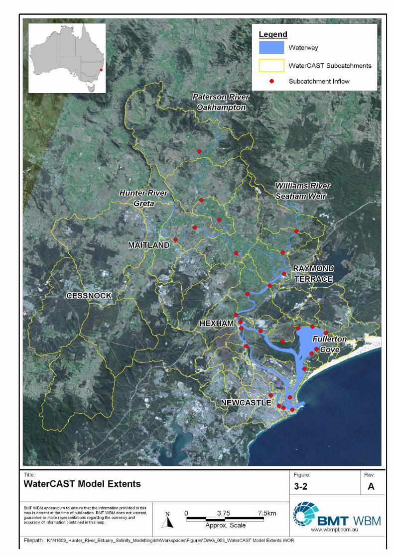
TUFLOW-FV model. The extent of the WaterCAST catchment model is shown in Figure 3-2.
3.5.3 Selection of inflow locations
An initial review of topographic data revealed numerous lateral inflows to the Patterson River,
Williams River and Hunter River. These lateral inflow locations were further reviewed and refined to
include inflows locations considered important to the hydrodynamic modelling component of the
project (i.e. locations where significant volumetric inputs would occur in the Hunter River estuary).
The final inflow locations adopted for the hydrodynamic model are shown in Figure 3-2.
3.5.4 Landuse mapping
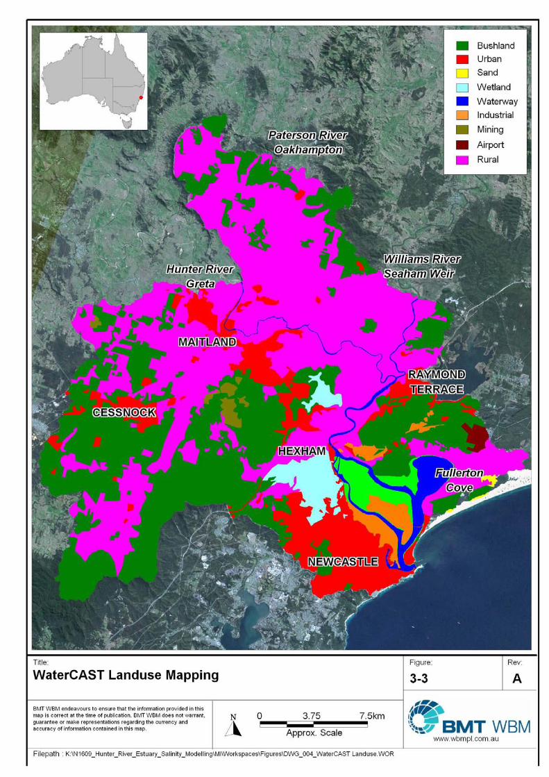
Satellite imagery was used to derive a landuse map of the study area. Landuse within the study area
was broadly classified according to the amount and type of impervious surfaces expected within. A
total of eight (8) landuse categories were identified and adopted in preparing the WaterCAST model
including:
Urban – Includes commercial, residential, open space areas common to the suburbs of
Newcastle (typical urban catchments);
Industrial and Airport – Includes highly impervious development such as the Kooragang and
Tomago Industrial areas, and Williamtown Airport;
Rural – Includes areas cleared of bushland / native vegetation but not urban development areas.
Some minor development (rural residential) expected within;
Bushland – Includes areas of uncleared native bushland;
Water – Includes the main waterways of the Hunter, Williams and Patterson River as well as
Grahamstown Dam and Fullerton Cove;
Wetland – Includes low-lying wetland areas identifiable from Satellite imagery such as Hexham
Swamp, Woodberry Swamp etc;
Mine – Includes small open cut mines located in some sub catchments; and
Sand – high pervious dunal areas fringing Stockton Bight.
These eight landuse categories were mapped in GIS (refer Figure 3-3) and used as input to the
WaterCAST catchment model in the form of an ASCII grid file. Areas of each landuse category within
individual subcatchments were automatically assigned by WaterCAST using the gridded input
dataset.
HYDRODYNAMIC MODEL DEVELOPMENT AND CALIBRATION 14
K:\N1609_HUNTER_RIVER_ESTUARY_SALINITY_MODELLING\DOCS\R.N1609.001.00.DOC
3.5.5 Rainfall-runoff model
The SIMHYD rainfall-runoff model was adopted for all landuse categories defined within the
WaterCAST model with the exception of waterway and mangrove areas. The TUFLOW-FV
hydrodynamic model has been configured to account for direct rainfall on these parts of the river
estuary and for this reason has been assigned no runoff within the WaterCAST catchment model.
Urban model rainfall-runoff parameters (other than the impervious area) were adopted from the
results of a NSW urban catchment calibration project that BMT WBM completed for the DECCW.
The adopted SIMHYD rainfall-runoff parameters are shown in Table 3-1 and are considered
representative for soil types situated within the urbanised catchment areas.
SIMHYD model parameters for non-urban catchment areas (e.g. bushland and rural) were estimated
from preliminary calibration of the SIMHYD rainfall-runoff model to stream flow records at Glen
Martin. SIMHYD is a conceptual rainfall-runoff model that is included within the Rainfall Runoff
Library (RRL), which is itself a simplified version of the daily conceptual rainfall-runoff model,
HYDROLOG, that was developed in 1972 and the more recent MODHYDROLOG. The RRL includes
a number of commonly used lumped rainfall runoff models, calibration optimisers and display tools to
facilitate hydrologic model calibration. RRL uses daily timeseries of rainfall, streamflow and
evapotranspiration data to estimate daily catchment runoff. The RRL currently contains 5 rainfall-
runoff models, 8 calibration optimisers, a choice of 10 objective functions and 3 types of data
transformation for comparison against observed data.
The RRL was used to calibrate the SIMHYD model to observed streamflow data and rainfall data in
the Williams River catchment, upstream of the gauging station at Glen Martin. The Williams River
catchment was considered to be a suitable representation of the non-urban catchment areas draining
to the Lower Hunter River Estuary due to similarities in its size, topography, landuse and proximity to
the study area. Streamflow data for Station 210010 (Glen Martin) was extracted for analysis from the
PINEENA database.
Streamflow gauging data at Station 210010 were available for the period 1974 to 2007 inclusive.
When calibrating continuous rainfall-runoff models such as SIMHYD, it is considered prudent to adopt
a calibration period that is representative of a ‘wet period’ where streamflow are typically higher.
Calibration of the rainfall-runoff model to a period of higher flows provides opportunity to capture more
runoff events and hence improves the robustness of the model following calibration. For this reason,
streamflow data for the period between January 1998 and December 2002 was chosen as the
calibration period. The calibration period was also chosen based upon the quality of the record (i.e.
record was continuous with no data gaps) and the availability of a corresponding rainfall record for the
same period.
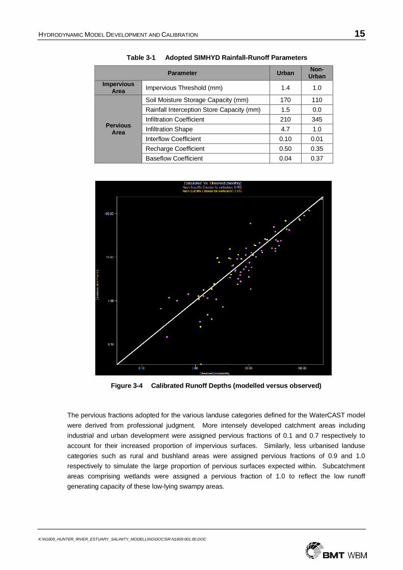
Catchment parameters estimated for the SIMHYD model during the preliminary calibration were
incorporated directly into the WaterCAST model and are shown in Table 3-1. A plot of the monthly
runoff depth is provided in Figure 3-4 and shows a very strong match (i.e. Nash-Sutcliffe Efficiency =
0.95) between the modelled discharge and observed runoff depths.
HYDRODYNAMIC MODEL DEVELOPMENT AND CALIBRATION 15
K:\N1609_HUNTER_RIVER_ESTUARY_SALINITY_MODELLING\DOCS\R.N1609.001.00.DOC
Table 3-1 Adopted SIMHYD Rainfall-Runoff Parameters
Parameter UrbanNon-
UrbanImpervious
Area Impervious Threshold (mm) 1.4 1.0
PerviousArea
Soil Moisture Storage Capacity (mm) 170 110
Rainfall Interception Store Capacity (mm) 1.5 0.0
Infiltration Coefficient 210 345
Infiltration Shape 4.7 1.0
Interflow Coefficient 0.10 0.01
Recharge Coefficient 0.50 0.35
Baseflow Coefficient 0.04 0.37
Figure 3-4 Calibrated Runoff Depths (modelled versus observed)
The pervious fractions adopted for the various landuse categories defined for the WaterCAST model
were derived from professional judgment. More intensely developed catchment areas including
industrial and urban development were assigned pervious fractions of 0.1 and 0.7 respectively to
account for their increased proportion of impervious surfaces. Similarly, less urbanised landuse
categories such as rural and bushland areas were assigned pervious fractions of 0.9 and 1.0
respectively to simulate the large proportion of pervious surfaces expected within. Subcatchment
areas comprising wetlands were assigned a pervious fraction of 1.0 to reflect the low runoff
generating capacity of these low-lying swampy areas.
HYDRODYNAMIC MODEL DEVELOPMENT AND CALIBRATION 16
K:\N1609_HUNTER_RIVER_ESTUARY_SALINITY_MODELLING\DOCS\R.N1609.001.00.DOC
3.5.6 Distribution of runoff volumes
WaterCAST is a daily catchment model that provides estimates of the daily runoff volume from a
modelled catchment. Runoff volumes estimated by WaterCAST at key locations draining into the
Lower Hunter River Estuary have been incorporated into the TUFLOW-FV hydrodynamic model as
inflows (refer Section 3.4.4). Average daily flow volumes (i.e. ML/day) estimated by WaterCAST
were used to define freshwater catchment inputs to the model, which are distributed evenly
throughout each day.
3.6 TULOW-FV Model Calibration
3.6.1 Boundary conditions
A number of boundary conditions have been assigned to the model to approximate the volume of
inflows entering the estuary from tides and river flows during the calibration of water level and salinity.
3.6.1.1 Water level
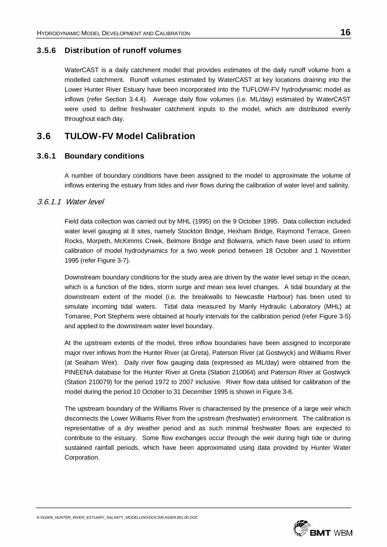
Field data collection was carried out by MHL (1995) on the 9 October 1995. Data collection included
water level gauging at 8 sites, namely Stockton Bridge, Hexham Bridge, Raymond Terrace, Green
Rocks, Morpeth, McKimms Creek, Belmore Bridge and Bolwarra, which have been used to inform
calibration of model hydrodynamics for a two week period between 18 October and 1 November
1995 (refer Figure 3-7).
Downstream boundary conditions for the study area are driven by the water level setup in the ocean,
which is a function of the tides, storm surge and mean sea level changes. A tidal boundary at the
downstream extent of the model (i.e. the breakwalls to Newcastle Harbour) has been used to
simulate incoming tidal waters. Tidal data measured by Manly Hydraulic Laboratory (MHL) at
Tomaree, Port Stephens were obtained at hourly intervals for the calibration period (refer Figure 3-5)
and applied to the downstream water level boundary.
At the upstream extents of the model, three inflow boundaries have been assigned to incorporate
major river inflows from the Hunter River (at Greta), Paterson River (at Gostwyck) and Williams River
(at Seaham Weir). Daily river flow gauging data (expressed as ML/day) were obtained from the
PINEENA database for the Hunter River at Greta (Station 210064) and Paterson River at Gostwyck
(Station 210079) for the period 1972 to 2007 inclusive. River flow data utilised for calibration of the
model during the period 10 October to 31 December 1995 is shown in Figure 3-6.
The upstream boundary of the Williams River is characterised by the presence of a large weir which
disconnects the Lower Williams River from the upstream (freshwater) environment. The calibration is
representative of a dry weather period and as such minimal freshwater flows are expected to
contribute to the estuary. Some flow exchanges occur through the weir during high tide or during
sustained rainfall periods, which have been approximated using data provided by Hunter Water
Corporation.
HYDRODYNAMIC MODEL DEVELOPMENT AND CALIBRATION 17
K:\N1609_HUNTER_RIVER_ESTUARY_SALINITY_MODELLING\DOCS\R.N1609.001.00.DOC
-1
-0.75
-0.5
-0.25
0
0.25
0.5
0.75
1
01-O
ct
03-O
ct
05-O
ct
07-O
ct
09-O
ct
11-O
ct
13-O
ct
15-O
ct
17-O
ct
19-O
ct
21-O
ct
23-O
ct
25-O
ct
27-O
ct
29-O
ct
31-O
ct
02-N
ov
04-N
ov
06-N
ov
08-N
ov
10-N
ov
12-N
ov
14-N
ov
16-N
ov
18-N
ov
20-N
ov
22-N
ov
24-N
ov
26-N
ov
28-N
ov
30-N
ov
02-D
ec
04-D
ec
06-D
ec
08-D
ec
10-D
ec
12-D
ec
14-D
ec
16-D
ec
18-D
ec
20-D
ec
22-D
ec
24-D
ec
26-D
ec
28-D
ec
30-D
ec
Wat
er L
evel
(m A
HD
)
Figure 3-5 Tidal Water Level Data
0
20
40
60
80
100
120
140
160
180
01-O
ct
03-O
ct
05-O
ct
07-O
ct
09-O
ct
11-O
ct
13-O
ct
15-O
ct
17-O
ct
19-O
ct
21-O
ct
23-O
ct
25-O
ct
27-O
ct
29-O
ct
31-O
ct
02-N
ov
04-N
ov
06-N
ov
08-N
ov
10-N
ov
12-N
ov
14-N
ov
16-N
ov
18-N
ov
20-N
ov
22-N
ov
24-N
ov
26-N
ov
28-N
ov
30-N
ov
02-D
ec
04-D
ec
06-D
ec
08-D
ec
10-D
ec
12-D
ec
14-D
ec
16-D
ec
18-D
ec
20-D
ec
22-D
ec
24-D
ec
26-D
ec
28-D
ec
30-D
ec
Flow
(m3 /
s)
Hunter River
Paterson River
Williams River
Figure 3-6 River Flow Data
HYDRODYNAMIC MODEL DEVELOPMENT AND CALIBRATION 18
K:\N1609_HUNTER_RIVER_ESTUARY_SALINITY_MODELLING\DOCS\R.N1609.001.00.DOC
3.6.1.2 Salinity
Salinity data were collected by Sanderson (2002) during the period 14 January 2001 to 3 April 2001.
Measurements of vertically averaged salinity were obtained using a hand-held water quality probe
(Yeo Kal) at approximately 20 to 30 locations between the entrance of Newcastle Harbour and
Raymond Terrace (via the North Arm of the Hunter River). These data provided an approximation of
the longitudinal salinity profile within this section of the Hunter River during the monitoring period.
Tidal data for Newcastle Harbour during the salinity calibration period were obtained from the
Newcastle Ports Corporation (NPC). The salinity concentration for the downstream tidal water level
was assumed to be a constant 35 ppt, however, it is noted that plumes of freshwater may extend
beyond the model boundary resulting salinity concentrations substantially lower than 35 ppt during
recovery from large flow events.
Major river inflows from the Hunter River and Paterson River were obtained using gauging records
available from the PINEENA database. Salinity data for the Hunter River were also available from
PINEENA database and have been included within the model. In the absence of salinity data for the
Paterson River, a nominal concentration of 0.25ppt was adopted by the model. An estimate of river
flow from the Williams River was obtained from HWC based on gauging records from Glen Martin,
water level gauging within the weir pool, records of weir gate operation, extraction of river flows to
Grahamstown Dam and modelled flows from upstream subcatchments. The data provided by HWC
represents the best available estimate of flow from the Williams River during the salinity calibration
period. Records of salinity concentrations for the Williams River were also unavailable during the
calibration period and a nominal concentration of 0.15 ppt was therefore adopted.
Freshwater inputs from subcatchments were included using daily estimates of runoff volume from the
WaterCAST catchment model. Again in the absence of any other data, a nominal salinity
concentration of 0.12ppt (approximately 200EC) was assumed for all freshwater catchment inputs.
Daily rainfall estimates obtained from synthetic timeseries data supplied by SILO at data drill location
near Hexham (latitude -32.80°, longitude 151.70°) for the calibration period were applied to the
surface of the model. Salinity concentration of rainfall was assumed to be 0ppt.
3.6.2 Results
3.6.2.1 Water levels
During calibration of model hydrodynamics, a number of variables were examined and adjusted to
ensure that model representation of wave propagation from the tidal signal was adequate and
reflective of observed conditions. The calibration focussed on representing bathymetry and surface
roughness conditions as best as possible throughout the study area, which have the greatest
influence on tidal hydrodynamics. The overall aim of the calibration was to achieve a good fit
between modelled and observed water levels including downstream sites within Newcastle Harbour
and upstream riverine sites between Raymond Terrace and Maitland.
A good calibration of hydrodynamics was achieved with the following hydrodynamic calibration values
(i.e. Manning’s ‘n’ roughness) and a global eddy viscosity parameter of 0.2m2/s:
HYDRODYNAMIC MODEL DEVELOPMENT AND CALIBRATION 19
K:\N1609_HUNTER_RIVER_ESTUARY_SALINITY_MODELLING\DOCS\R.N1609.001.00.DOC
Main waterway channels: n = 0.010;
Intertidal /mangrove areas: n = 0.100; and
Downstream tidal shoals areas: n = 0.030.
Discrepancies between observed and modelled water levels can be mostly attributed to errors in
defining the tidal prism resulting from less accurate and sparser bathymetry data in the upper river
sections of the model. Results of the water level calibration are presented in Figure 3-8.
3.6.2.2 Salinity
The presence of stratification (i.e. a 3D effect) within the deep Newcastle Harbour (near the
downstream boundary of the model) was evident within the measured data and identified as a key
process that may contribute to faster salt recovery following the freshwater event. It is important to
note that simulation of this process is not possible within the current 2-dimensional FVM (i.e.
stratification is a three dimensional process). Consequently, the salinity calibration sought to maintain
a good fit with salinity profiles under mostly ‘normal’ flow conditions rather than immediate post flood
conditions, which were demonstrably influenced by stratification and destratification processes in the
harbour.
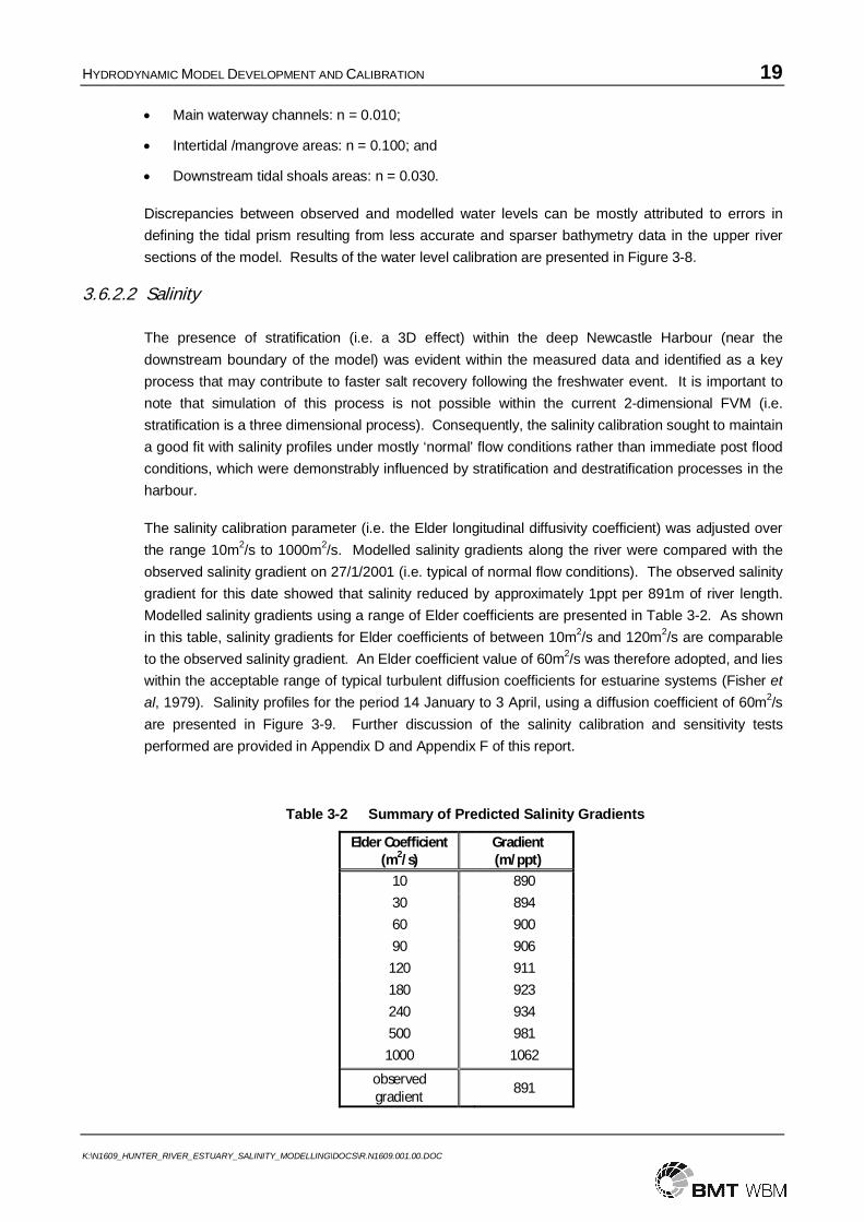
The salinity calibration parameter (i.e. the Elder longitudinal diffusivity coefficient) was adjusted over
the range 10m2/s to 1000m2/s. Modelled salinity gradients along the river were compared with the
observed salinity gradient on 27/1/2001 (i.e. typical of normal flow conditions). The observed salinity
gradient for this date showed that salinity reduced by approximately 1ppt per 891m of river length.
Modelled salinity gradients using a range of Elder coefficients are presented in Table 3-2. As shown
in this table, salinity gradients for Elder coefficients of between 10m2/s and 120m2/s are comparable
to the observed salinity gradient. An Elder coefficient value of 60m2/s was therefore adopted, and lies
within the acceptable range of typical turbulent diffusion coefficients for estuarine systems (Fisher et
al, 1979). Salinity profiles for the period 14 January to 3 April, using a diffusion coefficient of 60m2/s
are presented in Figure 3-9. Further discussion of the salinity calibration and sensitivity tests
performed are provided in Appendix D and Appendix F of this report.
Table 3-2 Summary of Predicted Salinity Gradients
Elder Coefficient(m2/s)
Gradient(m/ppt)
10 89030 89460 90090 906
120 911180 923240 934500 981
1000 1062
observed gradient
891
HYDRODYNAMIC MODEL DEVELOPMENT AND CALIBRATION 21
K:\N1609_HUNTER_RIVER_ESTUARY_SALINITY_MODELLING\DOCS\R.N1609.001.00.DOC
Figure 3-8 Water Level Calibration Results
HYDRODYNAMIC MODEL DEVELOPMENT AND CALIBRATION 22
K:\N1609_HUNTER_RIVER_ESTUARY_SALINITY_MODELLING\DOCS\R.N1609.001.00.DOC
Note: Blue line = measured data; green line = daily maximum; red line = daily minimum
Figure 3-9 Salinity Calibration Results Adopting an Elder coefficient of 60m2/s
SCENARIO MODELLING 23
K:\N1609_HUNTER_RIVER_ESTUARY_SALINITY_MODELLING\DOCS\R.N1609.001.00.DOC
4 SCENARIO MODELLING
4.1 Overview
The objective of the scenario modelling is to investigate the long-term salinity response within the
Hunter River estuary to modified flow regimes within the Hunter River, Paterson River and Williams
River. This has been undertaken utilising hydrodynamic and advection dispersion (AD) modelling to
simulate changes to salinity concentration at key locations between Newcastle Harbour and tidal
extents of the major upstream rivers.
The following key activities have been undertaken to achieve the objectives of the modelling:
Develop a two dimensional hydrodynamic model (TUFLOW-FV) of the Lower Hunter River
Estuary (refer Section 3.4 and Section 3.5);
Calibrate hydrodynamic (i.e. water level) and AD components (i.e. salinity) of the model to
measured data (refer Section 3.6); and
Simulate long-term conditions for a range of river flow modification scenarios defined by IQQM
modelling outputs (refer Section 4.2).
The key output of the scenario modelling is long-term timeseries of water level and salinity at key
locations within the lower Hunter River Estuary under modified flow conditions broadly representative
of ‘natural’, current and full development conditions. Comparison of outputs for these scenarios will
seek to identify the impact of the changed river flow conditions on salinity (particularly within the tidal
pool area). Results obtained for each of the modelling scenarios outlined below have been provided
to the NoW for analysis and interpretation by Dr Brian Williams.
A summary of key results are provided in Section 4.4.
4.2 Integrated Quantity and Quality Modelling (IQQM)
Timeseries data were provided by the NoW from the Hunter Integrated Quantity Quality Model
(IQQM) for input to the TUFLOW-FV model. Nine (9) model scenarios were simulated adopting a
range of development and flow rule conditions (i.e. natural, current and full development). Data
outputs from the Hunter IQQM comprise continuous daily timeseries of modelled river flow for the
period 1940 to 2007 at three locations, namely the Hunter River at Greta, Paterson River at Gostwyck
and the Williams River at Seaham Weir.
A summary of the scenarios simulated using TUFLOW-FV including a description and IQQM files
adopted is provided in Table 4-1. Timeseries of river flow inputs predicted by the IQQM model for the
Hunter River, Paterson River and Williams River is shown in Figure 4-2, Figure 4-3 and Figure 4-4
respectively.
SCENARIO MODELLING 24
K:\N1609_HUNTER_RIVER_ESTUARY_SALINITY_MODELLING\DOCS\R.N1609.001.00.DOC
Table 4-1 Summary of IQQM Modelling Scenarios and Output
Scenario DescriptionHunter River
Paterson River
Williams River
1“Natural” Pre development
flowGretanat.txt Gostnat.txt dsshwnat.txt
2aFull Development no flow
rulesGretafpp.txt Gostfpp.txt Dsshwcpp_gated.txt
2bFull Development WSP flow
rulesGretafep.txt Gostfep.txt Dsshwceu_gated.txt
2cFull Development no flow
rules, plus damGretafpp.txt Gostfpp.txt Dsshwcpp_gated_till.txt
2dFull Development WSP flow
rules, plus damGretafep.txt Gostfep.txt Dsshwceu_gated_till.txt
3aCurrent Development no
flow rulesGretacpp.txt Gostcpp.txt Dsshwcpp_gated.txt
3bCurrent Development no
flow rules, plus damGretacpp.txt Gostcpp.txt Dsshwcpp_gated_till.txt
3cCurrent Development WSP
flow rulesGretacep.txt Gostcep.txt Dsshwceu_gated.txt
3dCurrent Development WSP
flow rules, plus damGretacep.txt Gostcep.txt Dsshwceu_gated_till.txt
4.3 Boundary Conditions
4.3.1 Hydrodynamics
In addition to the river flow boundary conditions defined using outputs from the IQQM (refer
Section 4.2) each of the scenario models adopted the following boundary conditions for the period
1940 to 2007:
Downstream tide level – hourly prediction of water level based on tidal constituents presented in
the Australian National Tide Tables 2005 for Newcastle Harbour. The influence of storm surge
and weather conditions (i.e. low pressure / high pressure systems) is therefore absent (i.e.
astronomical tide conditions only) from the downstream boundary adopted by the scenario
models. Salinity concentration assumed to be constant at 35 ppt;
Catchment inputs – daily runoff volumes (ML/day) based on modelled output from the
WaterCAST model for 25 subcatchment outlets. Nominal salinity concentration of 0.12ppt
(approximately 200EC) assumed for all freshwater catchment inputs; and
Direct Rainfall / Evaporation – daily rainfall and evaporation estimates obtained from synthetic
timeseries data supplied by SILO at data drill location near Hexham (latitude -32.80°, longitude
151.70°). Evaporation from an open water body has been incorporated using the Morton (mlake)
estimate. Salinity concentration assumed to be 0ppt.
The boundary conditions outlined above remained constant between model scenarios with only
modification of river flow inputs undertaken to incorporate catchment development and flow rule
conditions modelled by the IQQM.
SCENARIO MODELLING 25
K:\N1609_HUNTER_RIVER_ESTUARY_SALINITY_MODELLING\DOCS\R.N1609.001.00.DOC
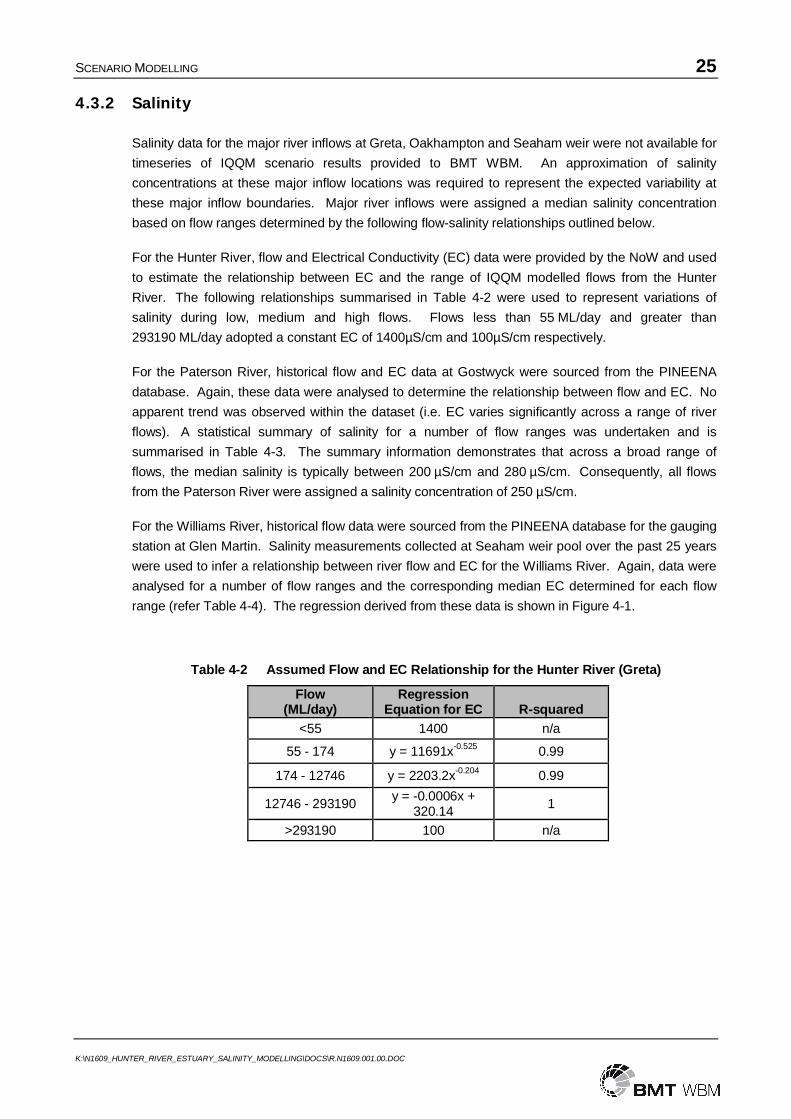
4.3.2 Salinity
Salinity data for the major river inflows at Greta, Oakhampton and Seaham weir were not available for
timeseries of IQQM scenario results provided to BMT WBM. An approximation of salinity
concentrations at these major inflow locations was required to represent the expected variability at
these major inflow boundaries. Major river inflows were assigned a median salinity concentration
based on flow ranges determined by the following flow-salinity relationships outlined below.
For the Hunter River, flow and Electrical Conductivity (EC) data were provided by the NoW and used
to estimate the relationship between EC and the range of IQQM modelled flows from the Hunter
River. The following relationships summarised in Table 4-2 were used to represent variations of
salinity during low, medium and high flows. Flows less than 55 ML/day and greater than
293190 ML/day adopted a constant EC of 1400µS/cm and 100µS/cm respectively.
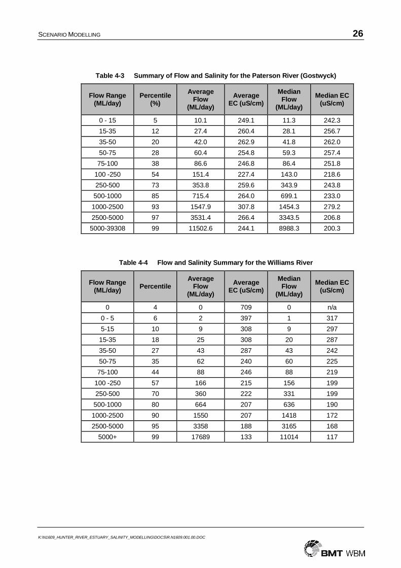
For the Paterson River, historical flow and EC data at Gostwyck were sourced from the PINEENA
database. Again, these data were analysed to determine the relationship between flow and EC. No
apparent trend was observed within the dataset (i.e. EC varies significantly across a range of river
flows). A statistical summary of salinity for a number of flow ranges was undertaken and is
summarised in Table 4-3. The summary information demonstrates that across a broad range of
flows, the median salinity is typically between 200 µS/cm and 280 µS/cm. Consequently, all flows
from the Paterson River were assigned a salinity concentration of 250 µS/cm.
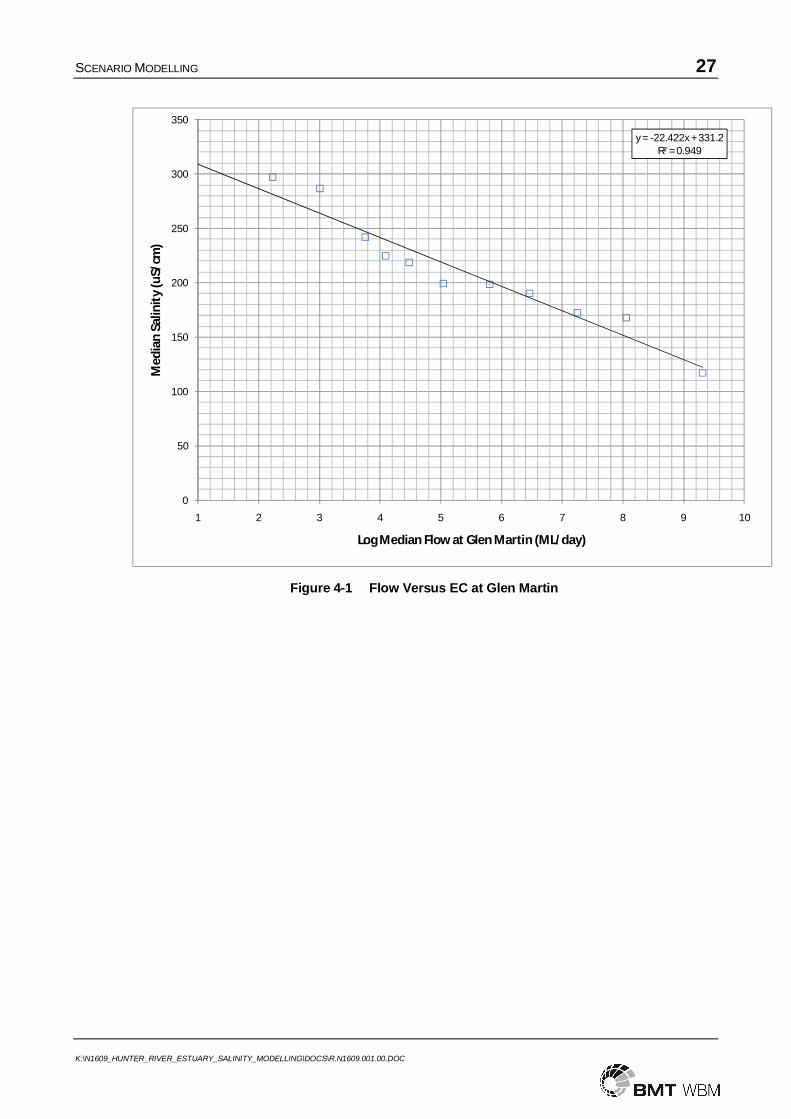
For the Williams River, historical flow data were sourced from the PINEENA database for the gauging
station at Glen Martin. Salinity measurements collected at Seaham weir pool over the past 25 years
were used to infer a relationship between river flow and EC for the Williams River. Again, data were
analysed for a number of flow ranges and the corresponding median EC determined for each flow
range (refer Table 4-4). The regression derived from these data is shown in Figure 4-1.
Table 4-2 Assumed Flow and EC Relationship for the Hunter River (Greta)
Flow(ML/day)
Regression Equation for EC R-squared
<55 1400 n/a
55 - 174 y = 11691x-0.525 0.99
174 - 12746 y = 2203.2x-0.204 0.99
12746 - 293190y = -0.0006x +
320.141
>293190 100 n/a
SCENARIO MODELLING 26
K:\N1609_HUNTER_RIVER_ESTUARY_SALINITY_MODELLING\DOCS\R.N1609.001.00.DOC
Table 4-3 Summary of Flow and Salinity for the Paterson River (Gostwyck)
Flow Range (ML/day)
Percentile(%)
Average Flow
(ML/day)
Average EC (uS/cm)
Median Flow
(ML/day)
Median EC (uS/cm)
0 - 15 5 10.1 249.1 11.3 242.3
15-35 12 27.4 260.4 28.1 256.7
35-50 20 42.0 262.9 41.8 262.0
50-75 28 60.4 254.8 59.3 257.4
75-100 38 86.6 246.8 86.4 251.8
100 -250 54 151.4 227.4 143.0 218.6
250-500 73 353.8 259.6 343.9 243.8
500-1000 85 715.4 264.0 699.1 233.0
1000-2500 93 1547.9 307.8 1454.3 279.2
2500-5000 97 3531.4 266.4 3343.5 206.8
5000-39308 99 11502.6 244.1 8988.3 200.3
Table 4-4 Flow and Salinity Summary for the Williams River
Flow Range (ML/day)
PercentileAverage
Flow (ML/day)
Average EC (uS/cm)
Median Flow
(ML/day)
Median EC (uS/cm)
0 4 0 709 0 n/a
0 - 5 6 2 397 1 317
5-15 10 9 308 9 297
15-35 18 25 308 20 287
35-50 27 43 287 43 242
50-75 35 62 240 60 225
75-100 44 88 246 88 219
100 -250 57 166 215 156 199
250-500 70 360 222 331 199
500-1000 80 664 207 636 190
1000-2500 90 1550 207 1418 172
2500-5000 95 3358 188 3165 168
5000+ 99 17689 133 11014 117
SCENARIO MODELLING 27
K:\N1609_HUNTER_RIVER_ESTUARY_SALINITY_MODELLING\DOCS\R.N1609.001.00.DOC
y = -22.422x + 331.2R² = 0.949
0
50
100
150
200
250
300
350
1 2 3 4 5 6 7 8 9 10
Med
ian
Salin
ity
(uS/
cm)
Log Median Flow at Glen Martin (ML/day)
Figure 4-1 Flow Versus EC at Glen Martin
SCENARIO MODELLING 28
K:\N1609_HUNTER_RIVER_ESTUARY_SALINITY_MODELLING\DOCS\R.N1609.001.00.DOC
Figure 4-2 River Flow Inputs from IQQM for the Hunter River
SCENARIO MODELLING 29
K:\N1609_HUNTER_RIVER_ESTUARY_SALINITY_MODELLING\DOCS\R.N1609.001.00.DOC
Figure 4-3 River Flow Inputs from IQQM for the Paterson River
SCENARIO MODELLING 30
K:\N1609_HUNTER_RIVER_ESTUARY_SALINITY_MODELLING\DOCS\R.N1609.001.00.DOC
Figure 4-4 River Flow Inputs from IQQM for the Williams River
SCENARIO MODELLING 31
K:\N1609_HUNTER_RIVER_ESTUARY_SALINITY_MODELLING\DOCS\R.N1609.001.00.DOC
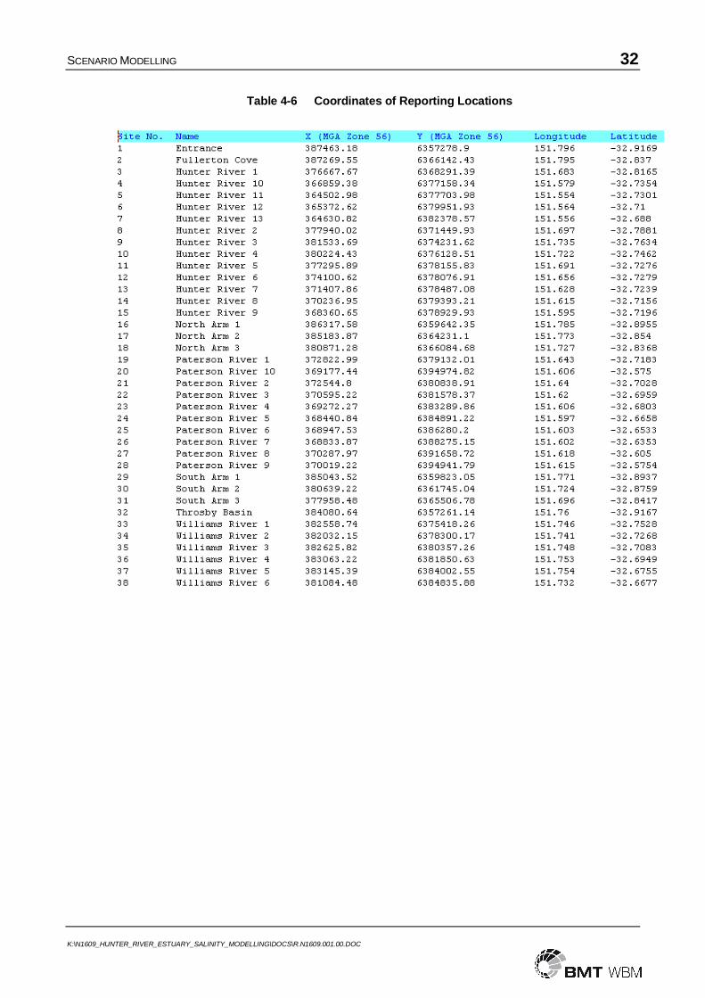
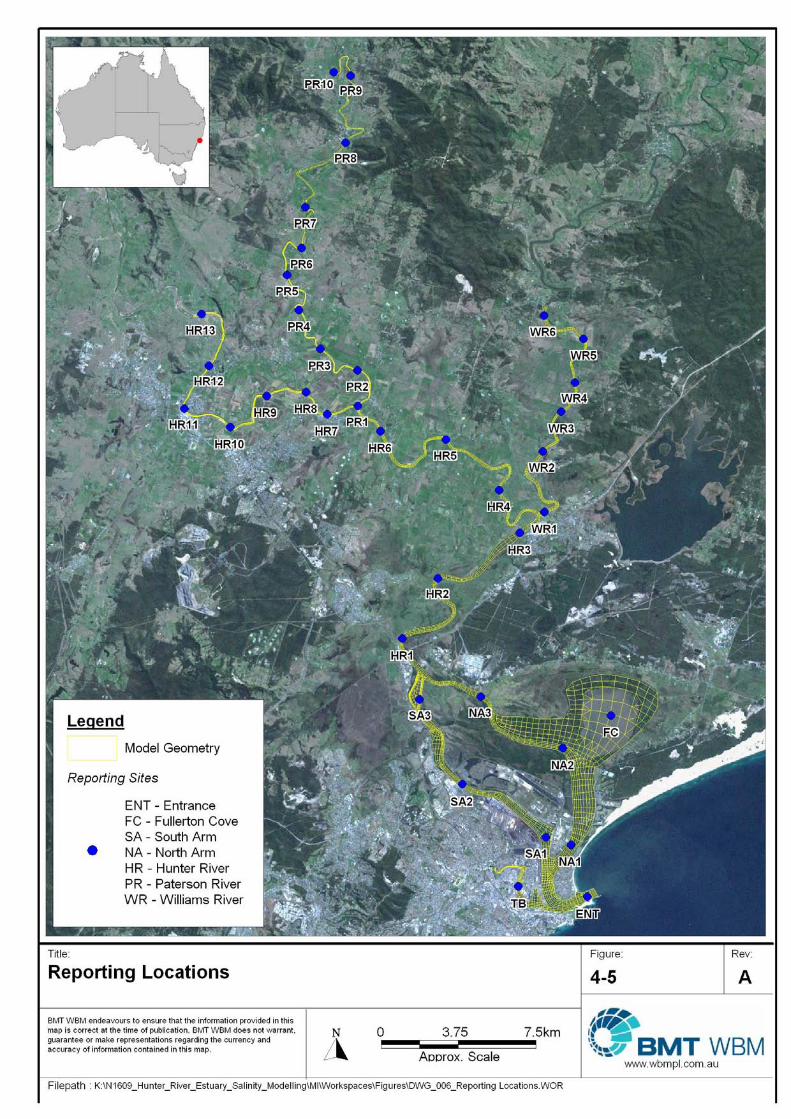
4.4 Results
The results of the long-term scenario modelling include the following variables and data formats for
38 reporting locations within the Hunter River Estuary (refer Table 4-6 and Figure 4-5).
1. Hourly estimates of water level, water depth, flow velocity and salinity for the period 1/1/1940 to
30/6/2007 in a csv file format; and
2. Spatial results of water level, water depth, flow velocity and salinity for the period 1/1/1940 to
30/6/2007 at 12 hour intervals in a binary dat file format.
In addition to the raw results outlined above, some post-processing of model results was undertaken
which includes extraction of daily maxima and minima water level and salinity at the 38 reporting
locations. An example of the output from the post-processing is shown in Table 4-5.
These data were provided to Dr Brian Williams for subsequent analysis, assessment and reporting.
Table 4-5 Sample Post-Processing Results
SCENARIO MODELLING 32
K:\N1609_HUNTER_RIVER_ESTUARY_SALINITY_MODELLING\DOCS\R.N1609.001.00.DOC
Table 4-6 Coordinates of Reporting Locations
CONCLUSIONS AND RECOMMENDATIONS 34
K:\N1609_HUNTER_RIVER_ESTUARY_SALINITY_MODELLING\DOCS\R.N1609.001.00.DOC
5 CONCLUSIONS AND RECOMMENDATIONS
Field investigations and data collected by Sanderson, Redden and Smith (2002) presents evidence of
stratification in the deeper sections of the harbour during the large freshwater flow event during the
calibration period. This information has been used to support the selection of an Elder coefficient
value of 60m2/s, which best matches longitudinal salinity profiles during ‘normal’ flow conditions, but
not the immediate post-fresh event (when other processes also influence salt dynamics in the
estuary).
The salinity calibration incorporates an improved estimate of flow from the Williams River which has
been shown to differ somewhat from gauging data obtained at Glen Martin (i.e. lag and attenuation of
peak flow is apparent between the gauging location and upstream boundary of model). The estimate
of river flow data used for the calibration of the TUFLOW-FV model represents the best data available
for the calibration period selected.
The calibration achieved using improved flow data for the Williams River and a salinity calibration
parameter (Elder coefficient) of 60m2/s is satisfactory for the purpose of assessing salinity response
over multi-decadal timescales. The calibrated FVM adequately reproduces observed longitudinal
salinity gradients measured between January and April 2001 and is comparable to the level of
calibration achieved by Sanderson (2005).
The nature of any modelling, particularly numerical modelling of complex waterways such as the
Hunter River Estuary is to generalise reality using assumptions or approximations of the key
processes important within a system. Long-term modelling assessments such as the approach
adopted by this study inherently make assumptions that relate to or are based upon current or
historical gauging periods (e.g. climate, river flow and ocean tides), and that these assumptions are
adequate to predict the response of a system to some change in the future. In such cases, an
assessment of the relative difference between model scenarios is undertaken to, for example, assess
and report on the relative changes in the estuary salinity structure between the identified water
sharing plan scenarios. Irrespective of assumptions surrounding long-term modelling, it is noted that
due to the lack of substantive salinity data for the upper reaches of the Hunter Estuary, further
investigations, analysis and IQQM modelling may be required to verify and / or further calibrate the
TUFLOW-FV model.
The following recommendations are therefore provided to address some of the current limitations of
the modelling undertaken for the current study:
1. Future monitoring to obtain observations of salinity concentration at the flow boundaries of
the model may assist with defining the concentration of salt entering the estuary and at key
locations within the upper reaches of the estuary for the purpose of comparing model
predictions during calibration;
2. To improve prediction of salinity response for scenario models, mass balance modelling of
salinity using the existing Hunter River IQQM is recommended. This would provide an
estimate of both river flow and salinity condition at the upstream extents of the TUFLOW-FV
model and would greatly reduce uncertainty of salinity estimates adopted by the model; and

CONCLUSIONS AND RECOMMENDATIONS 35
K:\N1609_HUNTER_RIVER_ESTUARY_SALINITY_MODELLING\DOCS\R.N1609.001.00.DOC
3. Development and calibration of a new catchment model may improve the temporal resolution
of inflow hydrographs adopted by the TUFLOW-FV model. Although the existing catchment
model provides an estimate of the daily, seasonal and inter-annual variation of rainfall and
runoff, an estimate of lateral inflows derived from sub-daily (e.g. hourly) rainfall-runoff
processes would better represent freshwater inputs to the system particularly for catchments
with a rapid rise and fall in flowrate (e.g. urban catchments) during individual rainfall events.
REFERENCES 36
K:\N1609_HUNTER_RIVER_ESTUARY_SALINITY_MODELLING\DOCS\R.N1609.001.00.DOC
6 REFERENCES
Fischer et al., 1979, Mixing in Inland and Coastal Waters, Academic Press, New York.
MHL 1995, Hunter River Estuary Data Collection 9 October 1995, Prepared by Department of Public
Works and Services Manly Hydraulics Laboratory, Report No. CFR96/02
MHL 2003, DLWC NSW Tidal Planes Data Compilation 2001 Volume 1 Tidal Plane Analyses, Report
MHL 1098, prepared for NSW Department of Land and Water Conservation, March 2003
Sanderson B., Redden R., Smith M., 2002, Salinity Structure of the Hunter River Estuary, Centre for
Sustainable Use of Coasts and Catchments, Ourimbah Campus, University of Newcastle.
Sanderson B. G., 2005, Changes in salinity structure of the Hunter River Estuary in response to
modified river flow, Prepared October 2005, University of Newcastle.
Sanderson B. G., 2007, Seasonal and Climatic Changes in salinity of the Hunter River Estuary in
Response to River Flow Modification by Environmental Flow Rules, Prepared March 2007, University
of Newcastle.

TUFLOW-FV MODEL DESCRIPTION A-1
K:\N1609_HUNTER_RIVER_ESTUARY_SALINITY_MODELLING\DOCS\R.N1609.001.00.DOC
APPENDIX A: TUFLOW-FV MODEL DESCRIPTION
EXISTING TUFLOW-FV DESCRIPTION A-1
G:\ADMIN\B16646.G.IAT\P.B16646.001.00.DOC
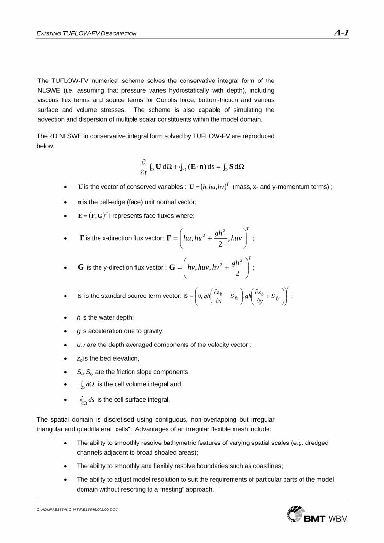
The TUFLOW-FV numerical scheme solves the conservative integral form of the
NLSWE (i.e. assuming that pressure varies hydrostatically with depth), including
viscous flux terms and source terms for Coriolis force, bottom-friction and various
surface and volume stresses. The scheme is also capable of simulating the
advection and dispersion of multiple scalar constituents within the model domain.
The 2D NLSWE in conservative integral form solved by TUFLOW-FV are reproduced
below,
∫ ∫=⋅+∫∂∂
Ω∂ ΩΩ dΩds)(dΩ SnEUt
• U is the vector of conserved variables : ( )Thvhuh ,,=U (mass, x- and y-momentum terms) ;
• n is the cell-edge (face) unit normal vector;
• ( )TGFE ,= i represents face fluxes where;
• F is the x-direction flux vector:
T
huvghhuhu ⎟⎟⎠
⎞⎜⎜⎝
⎛+= ,
2,
22F ;
• G is the y-direction flux vector :
Tghhvhuvhv ⎟⎟
⎠
⎞⎜⎜⎝
⎛+=
2,,
22G ;
• S is the standard source term vector:
T
fyb
fxb S
yz
ghSxz
gh ⎟⎟⎠
⎞⎜⎜⎝
⎛⎟⎟⎠
⎞⎜⎜⎝
⎛+
∂∂
⎟⎠
⎞⎜⎝
⎛ +∂∂
= ,,0S ;
• h is the water depth;
• g is acceleration due to gravity;
• u,v are the depth averaged components of the velocity vector ;
• zb is the bed elevation,
• Sfx,Sfy are the friction slope components
• ∫Ω Ωd is the cell volume integral and
• ∫ Ω∂ ds is the cell surface integral.
The spatial domain is discretised using contiguous, non-overlapping but irregular
triangular and quadrilateral “cells”. Advantages of an irregular flexible mesh include:
• The ability to smoothly resolve bathymetric features of varying spatial scales (e.g. dredged
channels adjacent to broad shoaled areas);
• The ability to smoothly and flexibly resolve boundaries such as coastlines;
• The ability to adjust model resolution to suit the requirements of particular parts of the model
domain without resorting to a “nesting” approach.
EXISTING TUFLOW-FV DESCRIPTION A-2
G:\ADMIN\B16646.G.IAT\P.B16646.001.00.DOC
The flexible mesh approach has significant benefits when applied to study
areas involving complex coastlines and embayments, varying bathymetries
and sharply varying flow and scalar concentration gradients.
A cell-centred spatial discretisation is currently employed in TUFLOW-FV, and
requires the calculation of numerical fluxes across cell boundaries. As with many
finite volume schemes non-viscous boundary fluxes are calculated using Roe’s
approximate Riemann solver (e.g. Glaister, 1988). The source terms due to bed
elevation changes between adjacent cells are “up-winded” as part of the Roe flux
solver, in order to maintain numerical consistency with the pressure gradient
momentum flux terms (Hubbard & Garcia-Navarro, 2000).
Viscous flux terms are calculated using the traditional gradient-diffusion model with a
variety of options available for the calculation of eddy-viscosity and scalar diffusivity.
The Smagorinksy eddy-viscosity model and the non-isotropic Elder diffusivity model
are the options most commonly adopted by BMT WBM modellers.
Both first-order and second-order spatial discretisation schemes are available in
TUFLOW-FV. The first-order scheme assumes a piecewise constant value of each
conservative constituent in a model cell. The second-order scheme assumes a 2D
linear polynomial reconstruction of the conservative constituents within the cell (i.e. a
MUSCL scheme). The Total Variation Diminishing (TVD) property (and hence
stability) of the solution is ensured using a choice of gradient limiter schemes.
The second-order spatial reconstruction scheme allows for much sharper resolution
of gradients in the conserved constituents for a given level of spatial resolution. This
is important for resolving relatively short waves (e.g. tsunamis) without excessive
numerical diffusion or without over-refining the spatial mesh discretisation. The
numerical resolution of sharply varying current distributions and sharp scalar
concentration fronts are also much improved with the second-order scheme.
Spatial integration is performed using a midpoint quadrature rule. Temporal
integration is performed with an explicit Euler scheme and must therefore maintain a
stable time step bounded by the Courant-Friedrich-Levy (CFL) criterion. A variable
time step scheme is implemented to ensure that the CFL criterion is satisfied with the
largest possible time step. Outputs providing information relating to performance of
the model with respect to the CFL criterion are provided to enable informed
refinement of the model mesh in accordance with the constraints of computational
time.
In very shallow regions (~<0.05m depth), the momentum terms are dropped, in order
to maintain stability as the NLSWE approach the zero-depth singularity. Mass
conservation is maintained both locally and globally to the limit of numerical precision
across the entire numerical domain, including wetting and drying fronts. A
conservative mass re-distribution scheme is used to ensure that negative depths are
avoided at numerically challenging wetting and drying fronts without recourse to
adjusting the time step. Regions of the model domain that are effectively dry are
readily dropped from the computations. Mixed sub/super-critical flow regimes are
EXISTING TUFLOW-FV DESCRIPTION A-3
G:\ADMIN\B16646.G.IAT\P.B16646.001.00.DOC
well handled by the FV scheme which intrinsically accounts for flow discontinuities
such as hydraulic jumps or bores that may occur in trans-critical flows.
Transport of scalar constituents is solved in a fully-coupled fashion with the NLWSE
solution. Simple linear decay and settling are optionally accommodated as
source/sink terms in the scalar transport equations.
TUFLOW-FV presently accommodates a wide variety of boundary conditions,
including those necessary for modelling the processes of importance to the present
study:
• Water level timeseries;
• In/out flow timeseries;
• Mean Sea Level Pressure gradients;
• Wind stress; and
• Wave radiation stress.
Bed friction is modelled using a Manning’s roughness formulation and Coriolis force
is also included in the model formulation.
The TUFLOW-FV engine leverages the parallel processing capabilities of modern
computer workstations, using the OpenMP implementation of shared memory
parallelism.
The model is currently fully operational as a 2D NLWSE solver, and development
work to extend the model to a 3D NLSWE solver including baroclinic forcing is being
planned.

Flexible MeshTUFLOW-FV (Finite Volume) isa hydrodynamic model enginewhich solves the Non-Linear Shallow Water Equations(NLSWE) on a "flexible" mesh comprising triangular and quadrilateral cells.
The flexible mesh approach has significant benefits when applied to study areas involving complex coastlines and embayments, varying bathymetries and sharply varying flow and scalar concentration gradients:
•Smoothly resolve bathymetric features of varying spatial scales;
•Smoothly and flexibly resolve boundaries such as coastlines;
•Adjust model resolution without resorting to a “nesting” approach.
BackgroundThe BMT WBM experience of using flexible mesh models, starting with the RMA finite-element models over a decade ago, has clearly demonstrated the benefits that they can deliver to complex coastal and estuarine modelling studies. The model “mesh” can be designed and constructed using various freely-available and proprietary software packages. The “SMS” package supplied by Aquaveo is routinely used byBMT WBM for the purpose of
Solution SchemeThe finite volume numerical scheme solves the conservative integral form of the NLSWE. The scheme is also capable of simulating the advection and dispersion of multiple scalar constituents within the model domain. Both first-order and second-order solution schemes are available for use. A 2D vertically-averaged scheme is operational and a 3D scheme is currently under development.
The TUFLOW-FV engine leverages the parallel processing capabilities of modern computer workstations, using the OpenMP implementation of shared memory parallelism. 64-bit, 8-core computers are now routinely used to deliver larger or longer model simulations.
Existing TUFLOW-FV Models:•Coral Sea and Great Barrier
Reef
•Persian Gulf
•South China Sea and Java Sea
•Port Curtis (various EIS assessments)
•Cairns Regional Council (storm tide inundation)
•Murray Mouth and Lower Lakes (salinity intrusion)
•Hunter River (salinity intrusion)
•South Alligator River (climate change impacts)
•Lihir Island (tsunami runup)
CapabilitiesSimilar to the original TUFLOW
model, the TUFLOW-FV model is
controlled via a fully-featured text-file
interface. This allows the user to
flexibly and efficiently control model
configuration, boundary condition
specification and output
requirements.
Closed (reflective) boundaries:
•Full-slip and no-slip conditions.
Open boundaries:
•Fully open (non-reflective).
•Specified water level.
•Specified discharge.
Miscellaneous forcing:
•Global cell inflows and outflows
(e.g. rainfall, evaporation).
•Cell inflows/outflows (e.g. pollutant
source/sinks).
•Wind stress.
•Atmospheric pressure.
•Wave radiation stress.
•Holland parametric cyclone wind
and pressure model is integrated
into the code.
•Various gridded forcing (e.g.
spatially and temporally varying
wind.
Additional Modules
•Cohesive Sediment Module
•Advection Dispersion
TUFLOWfv
A part of BMT in Energy and Environment
constructing generic modelmesh files.

NOW APPROVAL LETTER B-1
K:\N1609_HUNTER_RIVER_ESTUARY_SALINITY_MODELLING\DOCS\R.N1609.001.00.DOC
APPENDIX B: NOW APPROVAL LETTER
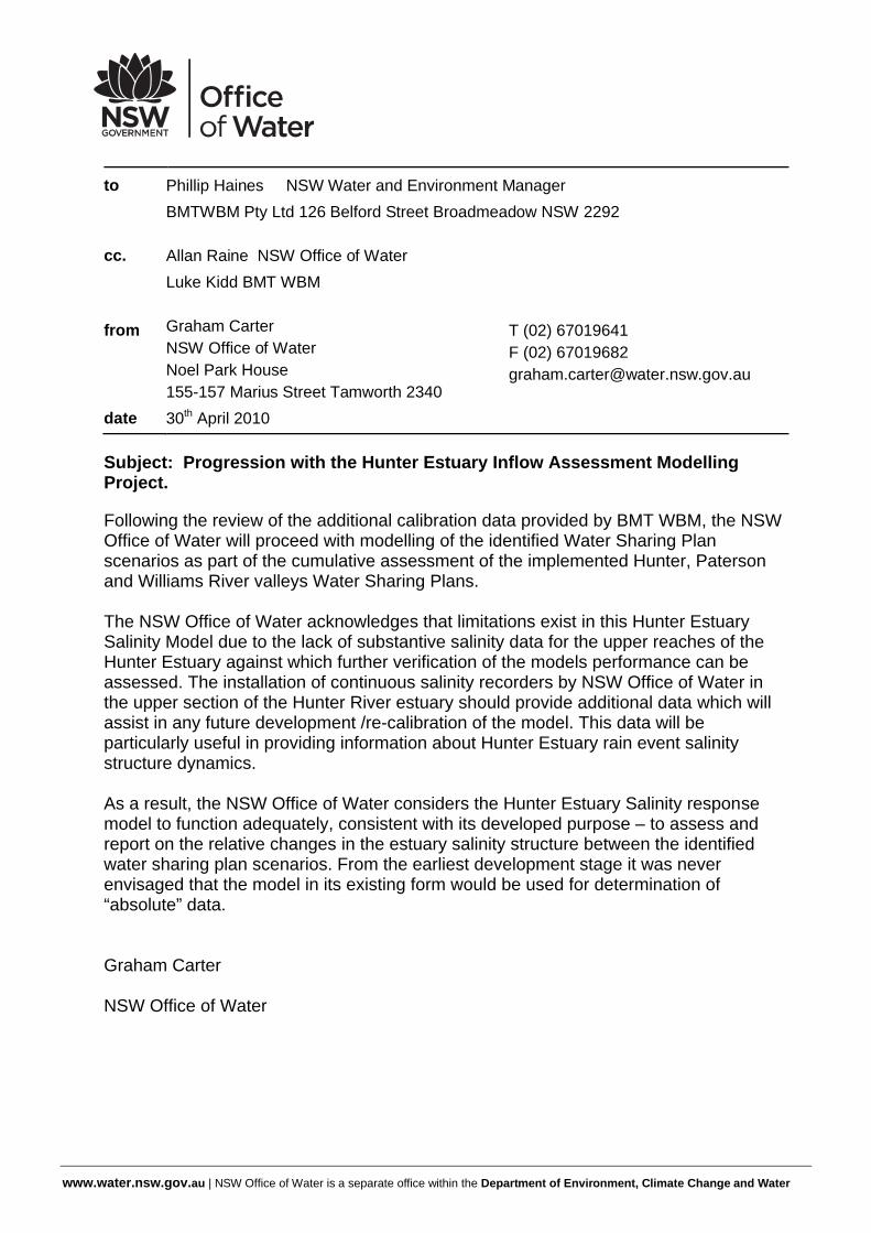
www.water.nsw.gov.au | NSW Office of Water is a separate office within the Department of Environment, Climate Change and Water
to Phillip Haines NSW Water and Environment Manager
BMTWBM Pty Ltd 126 Belford Street Broadmeadow NSW 2292
cc. Allan Raine NSW Office of Water
Luke Kidd BMT WBM
from Graham CarterNSW Office of Water Noel Park House155-157 Marius Street Tamworth 2340
T (02) 67019641F (02) [email protected]
date 30th April 2010
Subject: Progression with the Hunter Estuary Inflow Assessment Modelling Project.
Following the review of the additional calibration data provided by BMT WBM, the NSW Office of Water will proceed with modelling of the identified Water Sharing Plan scenarios as part of the cumulative assessment of the implemented Hunter, Paterson and Williams River valleys Water Sharing Plans.
The NSW Office of Water acknowledges that limitations exist in this Hunter Estuary Salinity Model due to the lack of substantive salinity data for the upper reaches of the Hunter Estuary against which further verification of the models performance can be assessed. The installation of continuous salinity recorders by NSW Office of Water in the upper section of the Hunter River estuary should provide additional data which will assist in any future development /re-calibration of the model. This data will be particularly useful in providing information about Hunter Estuary rain event salinity structure dynamics.
As a result, the NSW Office of Water considers the Hunter Estuary Salinity response model to function adequately, consistent with its developed purpose – to assess and report on the relative changes in the estuary salinity structure between the identified water sharing plan scenarios. From the earliest development stage it was never envisaged that the model in its existing form would be used for determination of “absolute” data.
Graham Carter
NSW Office of Water

SALINITY CALIBRATION LETTER 1 C-1
K:\N1609_HUNTER_RIVER_ESTUARY_SALINITY_MODELLING\DOCS\R.N1609.001.00.DOC
APPENDIX C: SALINITY CALIBRATION LETTER 1
K:\N1609_Hunter_River_Estuary_Salinity_Modelling\Docs\L.N1609.005.doc A part of BMT in Energy and Environment
BMT WBM Pty Ltd126 Belford StreetBROADMEADOW NSW 2292AustraliaPO Box 266Broadmeadow NSW 2292
Tel: +61 2 4940 8882Fax: +61 2 4940 8887
ABN 54 010 830 421 003
www.wbmpl.com.au
Our Ref: LJK: L.N1609.005.doc
7 January 2010
NSW Office of WaterPO Box 2213 Dangar NSW 2309
Attention: Eddie Harris / Graham Carter
Dear Eddie and Graham
RE: HUNTER RIVER SALINITY CALIBRATION
Further to our meeting with the NSW Office of Water and Hunter Water Corporation representatives on 23/12/09, we would like to provide you with an update of the calibration exercise undertaken to date.
Background
During the meeting, preliminary results were discussed, along with known data gaps and other key processes that may be contributing to differences between the observed data and modelled results. A number of important points were raised by NSW Office of Water (NOW) and BMT WBM regarding the salinity calibration and intended use of the Finite Volume Model (FVM), which are outlined below:
1. Small changes to salinity could have significant implications for licensed water users around the tidal pool;
2. Consideration of both the frequency and duration of salinity exceedance events is of particular interest to the NOW;
3. Flow data for contribution of freshwater from the Williams River at Seaham Weir should be used instead of the Glen Martin gauging data. The substantial catchment area downstream of the Glen Martin stream gauge and offtakes to Grahamstown Dam need to be accounted for with as much accuracy as possible;
4. HWC offered to assist with development of the model through the provision historical records of gate opening / closing relevant to the Seaham weir pool as well as an improved estimate of flow reaching Seaham Weir based on historical gauging at Glen Martin, pumping volumes at Balickera offtake and the additional contributing runoff volume (modelled) downstream of Glen Martin during the first few months of 2001;
5. Although preliminary model results presented at the meeting showed good agreement with measured salinity data, there remains some discrepancy between the observed data and modelled salt recovery following the freshwater event;
6. The salinity calibration parameter (i.e. the Elder longitudinal diffusivity coefficient) was adjusted over the range 10m2/s to 1000m2/s. Although a value of 1000m2/s provided an improved match between the observed and modelled post-fresh salt recovery, it was identified as being very high and that other processes (other than diffusion) were more likely to be contributing to the observed rapid salt recovery; and
7. The presence of stratification (i.e. a 3D effect) within the deep Newcastle Harbour (near the downstream boundary of the model) was identified as a key process that may contribute to faster salt recovery following the freshwater event. Simulation of this process is not possible within the current 2-dimensional FVM.
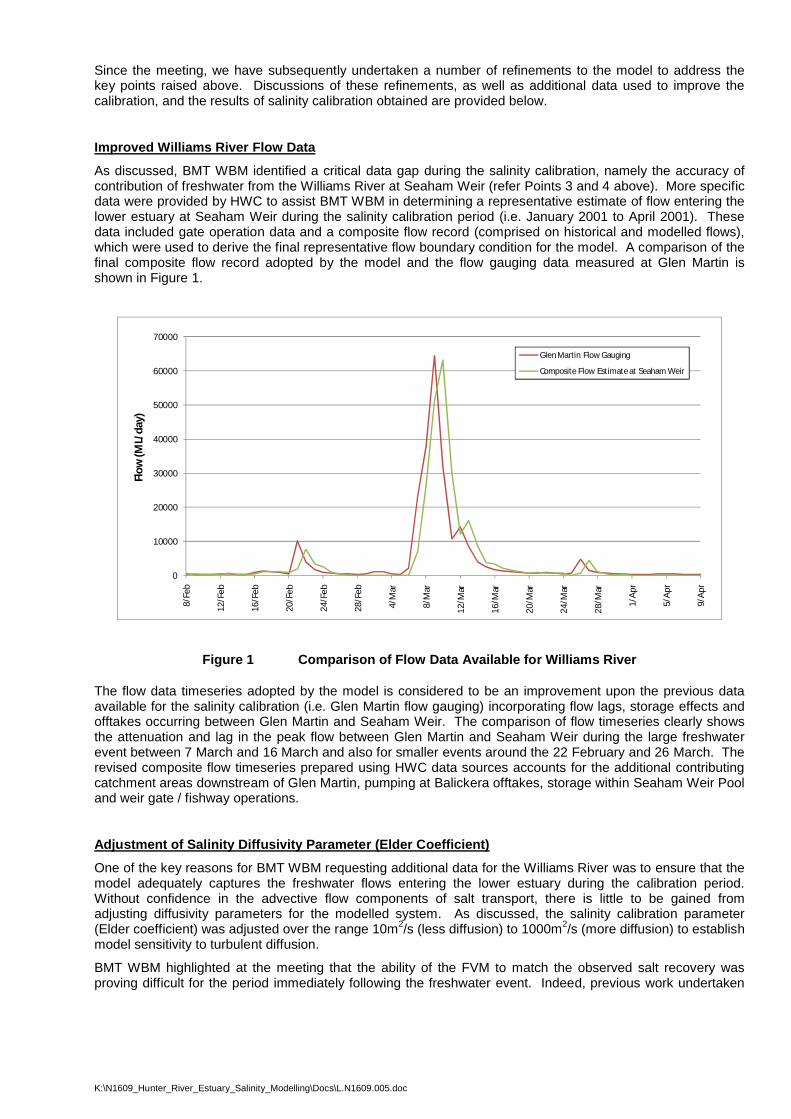
K:\N1609_Hunter_River_Estuary_Salinity_Modelling\Docs\L.N1609.005.doc
Since the meeting, we have subsequently undertaken a number of refinements to the model to address the key points raised above. Discussions of these refinements, as well as additional data used to improve the calibration, and the results of salinity calibration obtained are provided below.
Improved Williams River Flow Data
As discussed, BMT WBM identified a critical data gap during the salinity calibration, namely the accuracy of contribution of freshwater from the Williams River at Seaham Weir (refer Points 3 and 4 above). More specific data were provided by HWC to assist BMT WBM in determining a representative estimate of flow entering the lower estuary at Seaham Weir during the salinity calibration period (i.e. January 2001 to April 2001). These data included gate operation data and a composite flow record (comprised on historical and modelled flows), which were used to derive the final representative flow boundary condition for the model. A comparison of the final composite flow record adopted by the model and the flow gauging data measured at Glen Martin is shown in Figure 1.
0
10000
20000
30000
40000
50000
60000
70000
8/Fe
b
12/F
eb
16/F
eb
20/F
eb
24/F
eb
28/F
eb
4/M
ar
8/M
ar
12/M
ar
16/M
ar
20/M
ar
24/M
ar
28/M
ar
1/A
pr
5/A
pr
9/A
pr
Flow
(ML/
day)
Glen Martin Flow Gauging
Composite Flow Estimate at Seaham Weir
Figure 1 Comparison of Flow Data Available for Williams River
The flow data timeseries adopted by the model is considered to be an improvement upon the previous data available for the salinity calibration (i.e. Glen Martin flow gauging) incorporating flow lags, storage effects and offtakes occurring between Glen Martin and Seaham Weir. The comparison of flow timeseries clearly shows the attenuation and lag in the peak flow between Glen Martin and Seaham Weir during the large freshwater event between 7 March and 16 March and also for smaller events around the 22 February and 26 March. The revised composite flow timeseries prepared using HWC data sources accounts for the additional contributing catchment areas downstream of Glen Martin, pumping at Balickera offtakes, storage within Seaham Weir Pool and weir gate / fishway operations.
Adjustment of Salinity Diffusivity Parameter (Elder Coefficient)
One of the key reasons for BMT WBM requesting additional data for the Williams River was to ensure that the model adequately captures the freshwater flows entering the lower estuary during the calibration period. Without confidence in the advective flow components of salt transport, there is little to be gained from adjusting diffusivity parameters for the modelled system. As discussed, the salinity calibration parameter(Elder coefficient) was adjusted over the range 10m2/s (less diffusion) to 1000m2/s (more diffusion) to establish model sensitivity to turbulent diffusion.
BMT WBM highlighted at the meeting that the ability of the FVM to match the observed salt recovery was proving difficult for the period immediately following the freshwater event. Indeed, previous work undertaken
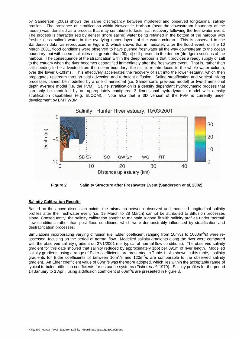
K:\N1609_Hunter_River_Estuary_Salinity_Modelling\Docs\L.N1609.005.doc
by Sanderson (2001) shows the same discrepancy between modelled and observed longitudinal salinity profiles. The presence of stratification within Newcastle Harbour (near the downstream boundary of the model) was identified as a process that may contribute to faster salt recovery following the freshwater event. The process is characterised by denser (more saline) water being retained in the bottom of the harbour with fresher (less saline) water in the overlying upper layers of the water column. This is observed in the Sanderson data, as reproduced in Figure 2, which shows that immediately after the flood event, on the 10 March 2001, flood conditions were observed to have pushed freshwater all the way downstream to the ocean boundary, but with ocean salinities (i.e. greater than 30ppt) still present in the deeper (dredged) sections of the harbour. The consequence of the stratification within the deep harbour is that it provides a ready supply of salt to the estuary when the river becomes destratified immediately after the freshwater event. That is, rather than salt needing to be advected from the ocean boundary, the salt is re-introduced to the whole water column, over the lower 6-10kms. This effectively accelerates the recovery of salt into the lower estuary, which then propagates upstream through tidal advection and turbulent diffusion. Saline stratification and vertical mixing processes cannot be modelled by a one dimensional (i.e. Sanderson’s previous model) or two-dimensional depth average model (i.e. the FVM). Saline stratification is a density dependant hydrodynamic process that can only be modelled by an appropriately configured 3-dimensional hydrodynamic model with density stratification capabilities (e.g. ELCOM). Note also that a 3D version of the FVM is currently under development by BMT WBM.
Figure 2 Salinity Structure after Freshwater Event (Sanderson et al, 2002)
Salinity Calibration Results
Based on the above discussion points, the mismatch between observed and modelled longitudinal salinity profiles after the freshwater event (i.e. 19 March to 28 March) cannot be attributed to diffusion processes alone. Consequently, the salinity calibration sought to maintain a good fit with salinity profiles under ‘normal’ flow conditions rather than post flood conditions, which were demonstrably influenced by stratification and destratification processes.
Simulations incorporating varying diffusion (i.e. Elder coefficient ranging from 10m2/s to 1000m2/s) were re-assessed, focusing on the period of normal flow. Modelled salinity gradients along the river were compared with the observed salinity gradient on 27/1/2001 (i.e. typical of normal flow conditions). The observed salinity gradient for this date showed that salinity reduced by approximately 1ppt per 891m of river length. Modelled salinity gradients using a range of Elder coefficients are presented in Table 1. As shown in this table, salinity gradients for Elder coefficients of between 10m2/s and 120m2/s are comparable to the observed salinity gradient. An Elder coefficient value of 60m2/s was therefore adopted, which lies within the acceptable range oftypical turbulent diffusion coefficients for estuarine systems (Fisher et al, 1979). Salinity profiles for the period 14 January to 3 April, using a diffusion coefficient of 60m2/s are presented in Figure 3.
K:\N1609_Hunter_River_Estuary_Salinity_Modelling\Docs\L.N1609.005.doc
Table 1 Summary of Predicted Salinity Gradients
Elder Coefficient(m2/s)
Gradient(m/ppt)
10 89030 89460 90090 906
120 911180 923240 934500 981
1000 1062
observed gradient 891
Conclusions
The information presented above has been provided to clarify a number of key points raised during the meeting. The calibration now incorporates an improved estimate of flow from the Williams River which has been shown to differ somewhat from the gauging data provided at Glen Martin (i.e. significant lag and some attenuation of peak flow volumes). The flow data used within the calibration of the FVM is considered to represent the best data available for the calibration period selected.
Further investigations and review of work undertaken by Sanderson et al (2002) provides evidence of stratification in the deeper sections of the harbour during the large freshwater flow event. This information has been used to support the selection of an Elder coefficient value of 60m2/s, which best matches longitudinal salinity profiles during ‘normal’ flow conditions, but not the immediate post-fresh event (when other processes also influence salt dynamics in the estuary).
We consider the calibration achieved using improved flow data for the Williams River and a salinity calibration parameter (Elder coefficient) of 60m2/s to be satisfactory for the purpose of assessing salinity response over multi-decadal timescales. The calibrated FVM adequately reproduces observed longitudinal salinity gradients measured between January and April 2001 and is comparable to the level of calibration achieved by Sanderson (2005).
We request that you formally acknowledge agreement to our calibration of the FVM, so that we can continue the flow scenarios previously requested by NOW without delay.
Should you have any questions regarding the above, please do not hesitate to contact me on 49408882.
Yours FaithfullyBMT WBM Pty Ltd
Luke KiddSenior Environmental Engineer

K:\N1609_Hunter_River_Estuary_Salinity_Modelling\Docs\L.N1609.005.doc
References
Sanderson et al (2002) Salinity Structure of the Hunter River Estuary, Centre for Sustainable Use of Coasts and Catchments, Ourimbah Campus, University of Newcastle.
Sanderson (2005) Changes in salinity of the Hunter Estuary in response to modified river flow, Prepared for Department of Infrastructure Planning and Natural Resources, 13 October 2005.
Fischer et al (1979) Mixing in Inland and Coastal Waters, Academic Press, New York.
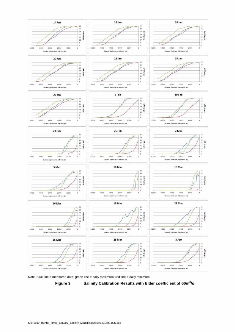
K:\N1609_Hunter_River_Estuary_Salinity_Modelling\Docs\L.N1609.005.doc
Note: Blue line = measured data; green line = daily maximum; red line = daily minimum
Figure 3 Salinity Calibration Results with Elder coefficient of 60m2/s

SALINITY CALIBRATION LETTER 2 D-1
K:\N1609_HUNTER_RIVER_ESTUARY_SALINITY_MODELLING\DOCS\R.N1609.001.00.DOC
APPENDIX D: SALINITY CALIBRATION LETTER 2
K:\N1609_Hunter_River_Estuary_Salinity_Modelling\Docs\L.N1609.006.docx A part of BMT in Energy and Environment
BMT WBM Pty Ltd 126 Belford Street BROADMEADOW NSW 2292 Australia PO Box 266 Broadmeadow NSW 2292 Tel: +61 2 4940 8882 Fax: +61 2 4940 8887 ABN 54 010 830 421 003 www.wbmpl.com.au
Our Ref: LJK: L.N1609.006.docx 24 February 2010 NSW Office of Water Tamworth Office PO Box 550 Tamworth NSW 2340 Attention: Graham Carter Dear Graham RE: HUNTER RIVER SALINITY MODELLING – PROGRESS OF SALINITY CALIBRATION
Thank you for your recent email dated 3 February 2010 regarding progress of salinity calibration for the Hunter River Salinity Modelling project. Following our telephone conversation yesterday, we wish to clarify some aspects of the salinity calibration with the NSW Office of Water (NOW) and justification of the salinity calibration carried out thus far. Please also find attached results (excel spreadsheets) of the salinity calibration using Elder coefficients of 10 and 60 as requested.
Background
Our previous correspondence letter (dated 7 January) outlined a number of refinements to the model including adoption of improved Williams River flow data and adjustment of the salinity diffusivity parameter (Elder coefficient). During the meeting other important items were discussed regarding use of our TUFLOW-FV model by Hunter Water Corporation (HWC), which included:
HWC has offered to assist with development of the model through the provision of data relevant to Seaham Weir. More accurate data from the Williams River at Seaham Weir (instead of the Glen Martin gauge data) could improve the model performance as there is a substantial catchment area downstream of the gauge.
HWC made no claim in regards to Intellectual Property through the provision of data (i.e. use is given unconditionally for development of the TUFLOW-FV model, but not to be used for any other purpose);
BMT WBM, NOW and DECCW agreed for HWC to commission work using the TUFLOW-FV model; and
It was agreed that any work commissioned by HWC should relate to pre and post Tillegra Dam investigations. Any other scenario testing for general water management purposes was beyond the scope of investigations being assessed by HWC.
The above items were discussed in a meeting with representatives from BMT WBM, NOW, DECCW and HWC and subsequently summarised in an email from HWC dated 23 December 2009.
Salinity Mixing Model (Elder Coefficient)
As previously discussed, the Elder coefficient was adjusted over the range 10 (less diffusion) to 1000 (more diffusion) to establish model sensitivity to turbulent diffusion. It should be noted that our previous correspondence reported erroneous units of m2/s for the Elder coefficient. In fact, the Elder coefficient is dimensionless and is used by the TUFLOW-FV to calculate a diffusivity value (K) which has units of m2/s.
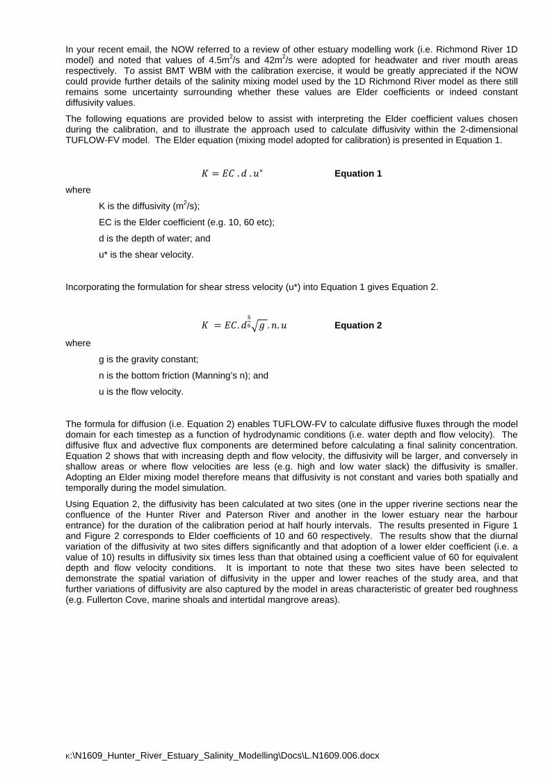
K:\N1609_Hunter_River_Estuary_Salinity_Modelling\Docs\L.N1609.006.docx
In your recent email, the NOW referred to a review of other estuary modelling work (i.e. Richmond River 1D model) and noted that values of 4.5m2/s and 42m2/s were adopted for headwater and river mouth areas respectively. To assist BMT WBM with the calibration exercise, it would be greatly appreciated if the NOW could provide further details of the salinity mixing model used by the 1D Richmond River model as there still remains some uncertainty surrounding whether these values are Elder coefficients or indeed constant diffusivity values.
The following equations are provided below to assist with interpreting the Elder coefficient values chosen during the calibration, and to illustrate the approach used to calculate diffusivity within the 2-dimensional TUFLOW-FV model. The Elder equation (mixing model adopted for calibration) is presented in Equation 1.
. . Equation 1
where
K is the diffusivity (m2/s);
EC is the Elder coefficient (e.g. 10, 60 etc);
d is the depth of water; and
u* is the shear velocity.
Incorporating the formulation for shear stress velocity (u*) into Equation 1 gives Equation 2.
. . . Equation 2
where
g is the gravity constant;
n is the bottom friction (Manning’s n); and
u is the flow velocity.
The formula for diffusion (i.e. Equation 2) enables TUFLOW-FV to calculate diffusive fluxes through the model domain for each timestep as a function of hydrodynamic conditions (i.e. water depth and flow velocity). The diffusive flux and advective flux components are determined before calculating a final salinity concentration. Equation 2 shows that with increasing depth and flow velocity, the diffusivity will be larger, and conversely in shallow areas or where flow velocities are less (e.g. high and low water slack) the diffusivity is smaller. Adopting an Elder mixing model therefore means that diffusivity is not constant and varies both spatially and temporally during the model simulation.
Using Equation 2, the diffusivity has been calculated at two sites (one in the upper riverine sections near the confluence of the Hunter River and Paterson River and another in the lower estuary near the harbour entrance) for the duration of the calibration period at half hourly intervals. The results presented in Figure 1 and Figure 2 corresponds to Elder coefficients of 10 and 60 respectively. The results show that the diurnal variation of the diffusivity at two sites differs significantly and that adoption of a lower elder coefficient (i.e. a value of 10) results in diffusivity six times less than that obtained using a coefficient value of 60 for equivalent depth and flow velocity conditions. It is important to note that these two sites have been selected to demonstrate the spatial variation of diffusivity in the upper and lower reaches of the study area, and that further variations of diffusivity are also captured by the model in areas characteristic of greater bed roughness (e.g. Fullerton Cove, marine shoals and intertidal mangrove areas).
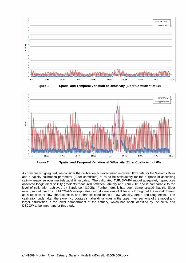
K:\N1609_Hunter_River_Estuary_Salinity_Modelling\Docs\L.N1609.006.docx
Figure 1 Spatial and Temporal Variation of Diffusivity (Elder Coefficient of 10)
Figure 2 Spatial and Temporal Variation of Diffusivity (Elder Coefficient of 60)
As previously highlighted, we consider the calibration achieved using improved flow data for the Williams River and a salinity calibration parameter (Elder coefficient) of 60 to be satisfactory for the purpose of assessing salinity response over multi-decadal timescales. The calibrated TUFLOW-FV model adequately reproduces observed longitudinal salinity gradients measured between January and April 2001 and is comparable to the level of calibration achieved by Sanderson (2005). Furthermore, it has been demonstrated that the Elder mixing model used by TUFLOW-FV incorporates diurnal variations of diffusivity throughout the model domain as a function of flow characteristics and channel condition (i.e. flow velocity, depth and roughness). The calibration undertaken therefore incorporates smaller diffusivities in the upper river sections of the model and larger diffusivities in the lower compartment of the estuary, which has been identified by the NOW and DECCW to be important for this study.

K:\N1609_Hunter_River_Estuary_Salinity_Modelling\Docs\L.N1609.006.docx
It would be greatly appreciated if the NOW and DECCW could provide comment on the above information as soon as possible so that the scenario modelling can be completed and our role in this project finalised. Should you have any questions regarding the above, please do not hesitate to contact me on 4940 8882.
Yours Faithfully BMT WBM Pty Ltd
Luke Kidd Senior Environmental Engineer

NOW REQUEST FOR ADDITIONAL INFORMATION E-1
K:\N1609_HUNTER_RIVER_ESTUARY_SALINITY_MODELLING\DOCS\R.N1609.001.00.DOC
APPENDIX E: NOW REQUEST FOR ADDITIONAL INFORMATION
Calibration and Verification of Hunter River model
In considering the calibration modelling to date and given that the model is new, the weak sensitivity of the dispersion to Elder coefficient variation leads to the following questions:
1. How does the model account for dispersion?
Our information to date suggests that Elder’s equation is used to estimate a longitudinal dispersivity constant from the Manning equation and a computed longitudinal stream velocity. How is transverse diffusivity determined? It will impact on transverse mixing and lead to greater or less shear dispersion. Given that the explanation of the insensitivity may lie in dominant transverse shear dispersion, it would be interesting to see some plan view plots of transverse velocity profiles and salinity. Activity at bends may also add to our understanding of the river/model’s behaviour.
2. Is the model dispersion sensitive to the size of the grid?The underlying mixing processes (longitudinal, transverse and vertical diffusivities) in the model are sub-grid-scale and their magnitude is grid-size dependent. How does the model account for this? Has the model’s dispersion output been shown to be independent of grid resolution?
3. Has the model’s performance been compared with analytical results or that of an existing model?
Has the model been compared to analytical results of simple cases of dispersion?We recognize that different numerical schemes may lead to diffusive numerical artifacts and such comparisons may need to be considered and discussed carefully. Have comparisons been made with dispersion simulations using other 2D models formerly used by WBM (not necessarily of the Hunter, but a system not dissimilar, with bends, deep channels etc)?
Can WBM BMT provide a response to these questions.
Graham CarterNSW Office of Water 4th March 2010

MEMORANDUM OF ADDITIONAL INFORMATION F-1
K:\N1609_HUNTER_RIVER_ESTUARY_SALINITY_MODELLING\DOCS\R.N1609.001.00.DOC
APPENDIX F: MEMORANDUM OF ADDITIONAL INFORMATION
K:\N1609_Hunter_River_Estuary_Salinity_Modelling\Docs\M.N1609.001.doc
From: BMT WBM To: Graham Carter; Eddie Harris; Mark Simons; John Floyd; Brian Williams
Date: 22 April 2010 CC:
Subject: Hunter River Salinity Modelling Sensitivity Tests
Introduction
In a letter dated 4 March 2010, the NOW highlighted the following two key questions:
1. How does the model account for dispersion?
2. Is the model dispersion sensitive to the size of the grid?
In a previous response by BMT WBM the following information was provided to the NOW:
“The model is a two dimensional depth-averaged hydrodynamic model. Velocity calculated by the model is a depth-averaged but in reality the top of the water column moves faster than the bottom (i.e. typically follows a logarithmic profile with velocity increasing with decreasing flow depth). The model therefore needs to account for shear dispersion in the principal direction of flow and this is done in the model of the Hunter River using the Elder equation and a coefficient of 60. Lateral shear dispersion is caused by eddies formed between streamlines where velocity varies across channel. Eddies cause lateral shear dispersion and dispersive fluxes to occur perpendicular to the longitudinal flux and this is accounted for in the model of the Hunter River using an Elder coefficient of 6. The use of the Elder equation to calculate longitudinal and transverse diffusivity coefficients is described in Falconer, R.A., Lin, B. and Kashefipour, S.M. (2005) Modelling Water Quality Processes in Estuaries Computational Fluid Dynamics: Applications in Environmental Hydraulics, Eds P.B. Bates, S.N. Lane and R.I. Furguson. John Wiley and Sons.”
“In any numerical advection-diffusion model the total model diffusion is comprised of the “specified” diffusion component and a “numerical” component, with the latter typically having a grid-size dependency, i.e. greater numerical diffusion with coarser grid sizes. Ideally the numerical diffusion component will be small relative to the advection and “specified” diffusion components of constituent transport. In TUFLOW-FV the spatial order of the solution scheme can be set as second order which significantly reduces numerical diffusion at the cost of greater computational effort and longer simulation times.”
The purpose of this meeting is to assess and review calibration data of the two-dimensional hydrodynamic model developed for the Hunter River Estuary and provide a response to these two key questions. As noted by the NSW Office of Water (NOW), the Hunter River Estuary model being reviewed is to be used to assist with the assessment of combined impacts from implementation of Hunter Catchment Water Sharing Plans on the salinity structure of the Hunter River Estuary.
The intent of this memorandum and subsequent information contained within is to summarise investigations carried out by BMT WBM and to facilitate discussions between representatives of NOW and DECCW.
Memorandum
K:\N1609_Hunter_River_Estuary_Salinity_Modelling\Docs\M.N1609.001.doc
Objectives
The objectives of the sensitivity testing were to:
a. Investigate the apparent insensitivity of Elder coefficient(s);
b. Verify that the relative insensitivity of coefficients used by the scalar mixing model can be explained by dispersive mixing process caused by across channel variations of velocity which are explicitly accounted for in the two dimensional hydrodynamic model;
c. Demonstrate that the magnitude of velocity predictions across the channel will differ for a uniform channel and a channel with shallow banks or a bench;
d. Demonstrate the change in salinity estimates using a longitudinal Elder coefficient of 10, 60, 120, 240 and 500; and
e. Demonstrate the change in salinity estimates using increased model resolution (i.e. 4 cells or 8 cells);
Methodology
Model Configuration
The following model parameters / configuration have been adopted for all sensitivity tests:
Model simulated for 336 hours (or 2 weeks);
A single boundary condition defined as a water level timeseries (using tidal data available Newcastle Harbour);
A single material type with a Manning’s n roughness of 0.010;
Momentum mixing model is Smagorinsky with a coefficient of 0.2;
Initial water level set to 0.4 m AHD to coincide with start of water level boundary condition;
Initial salinity within model domain was 0 ppt; and
Salinity of 1 ppt applied at water level boundary.
Model Geometry
A small section of the Hunter River North Arm was used as the basis for establishing model geometry for the sensitivity tests. The scale of the adopted model geometry is considered appropriate in the context of the study area. The model geometry used for the sensitivity tests is approximately 2200 meters long and 250 metres wide.
It is important to note that a comparative assessment has been used to assess the relative difference in model predictions. That is, the sensitivity tests carried out do not directly represent the Hunter River Estuary, but rather, are hypothetical model simulations that use generalised channel geometries to demonstrate the influence of adjusting model parameters (i.e. the Elder coefficient(s)) and model resolution (i.e. the number of cells used to define the geometry across the channel).
The sensitivity of model resolutions has been assessed using 4 cells and 8 cells across the width of the channel as shown in Figure 1. Three generalised channel geometries have been defined, namely a trapezoidal channel, uniform channel and shallow bench trapezoidal channel. Cross section profiles of these three channel types are shown in Figure 2.
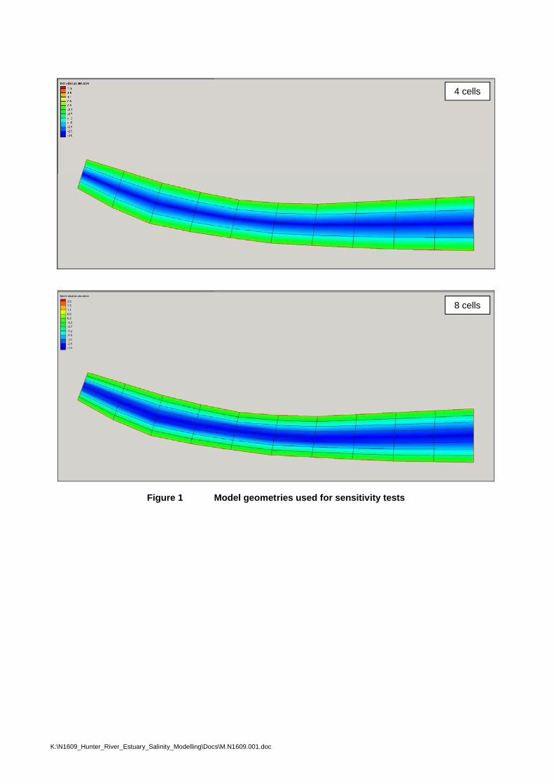
K:\N1609_Hunter_River_Estuary_Salinity_Modelling\Docs\M.N1609.001.doc
4 cells
Figure 1 Model geometries used for sensitivity tests
8 cells
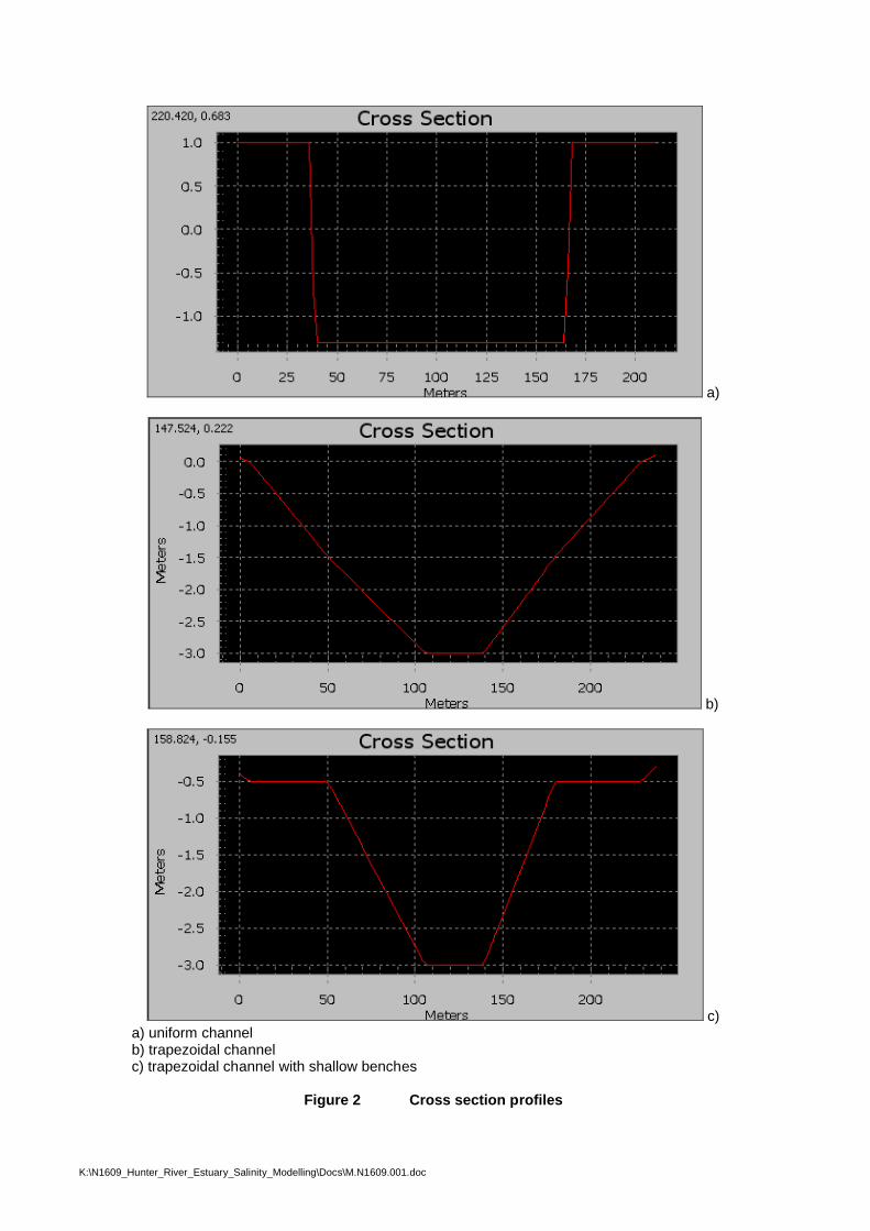
K:\N1609_Hunter_River_Estuary_Salinity_Modelling\Docs\M.N1609.001.doc
a)
b)
c)a) uniform channelb) trapezoidal channelc) trapezoidal channel with shallow benches
Figure 2 Cross section profiles
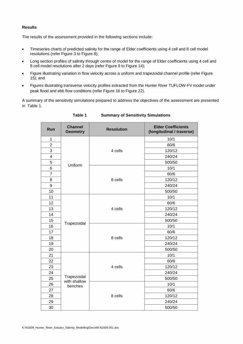
K:\N1609_Hunter_River_Estuary_Salinity_Modelling\Docs\M.N1609.001.doc
Results
The results of the assessment provided in the following sections include:
Timeseries charts of predicted salinity for the range of Elder coefficients using 4 cell and 8 cell model resolutions (refer Figure 3 to Figure 8);
Long section profiles of salinity through centre of model for the range of Elder coefficients using 4 cell and 8 cell model resolutions after 2 days (refer Figure 9 to Figure 14);
Figure illustrating variation in flow velocity across a uniform and trapezoidal channel profile (refer Figure 15); and
Figures illustrating transverse velocity profiles extracted from the Hunter River TUFLOW-FV model under peak flood and ebb flow conditions (refer Figure 16 to Figure 22).
A summary of the sensitivity simulations prepared to address the objectives of the assessment are presented in Table 1.
Table 1 Summary of Sensitivity Simulations
RunChannel
GeometryResolution
Elder Coefficients(longitudinal / traverse)
1
Uniform
4 cells
10/1
2 60/6
3 120/12
4 240/24
5 500/50
6
8 cells
10/1
7 60/6
8 120/12
9 240/24
10 500/50
11
Trapezoidal
4 cells
10/1
12 60/6
13 120/12
14 240/24
15 500/50
16
8 cells
10/1
17 60/6
18 120/12
19 240/24
20 500/50
21
Trapezoidal with shallow
benches
4 cells
10/1
22 60/6
23 120/12
24 240/24
25 500/50
26
8 cells
10/1
27 60/6
28 120/12
29 240/24
30 500/50
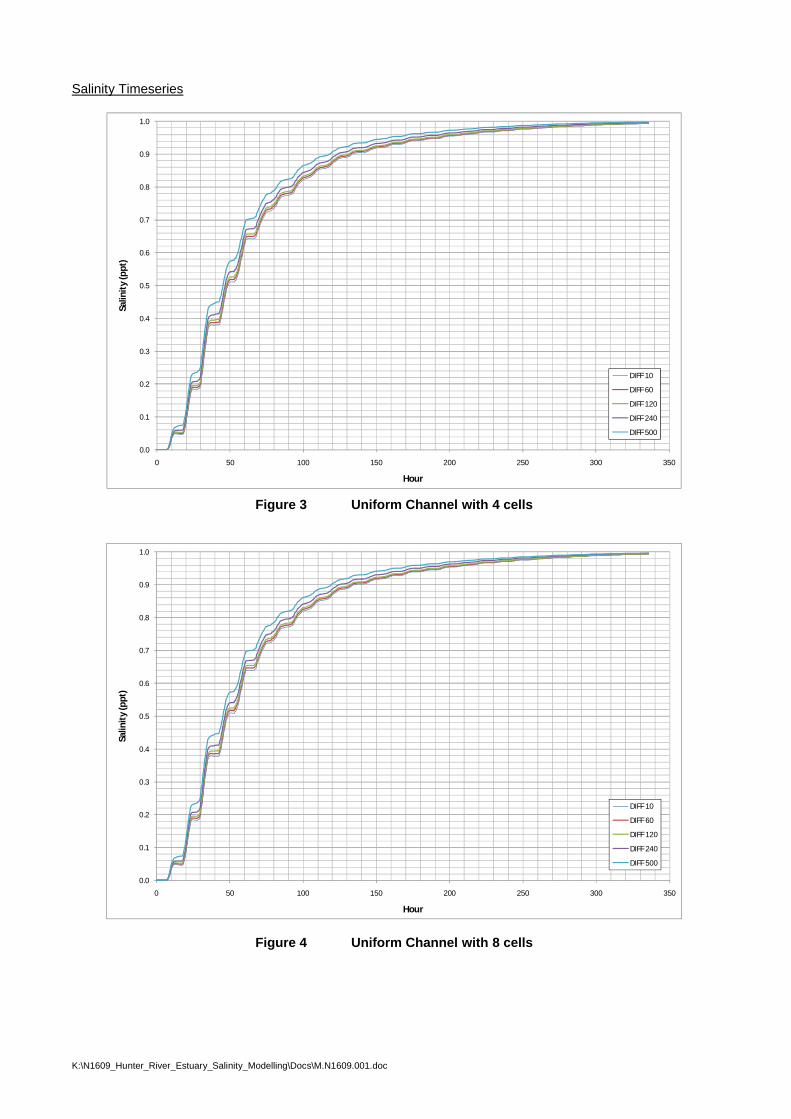
K:\N1609_Hunter_River_Estuary_Salinity_Modelling\Docs\M.N1609.001.doc
Salinity Timeseries
0.0
0.1
0.2
0.3
0.4
0.5
0.6
0.7
0.8
0.9
1.0
0 50 100 150 200 250 300 350
Salin
ity
(ppt
)
Hour
DIFF 10
DIFF 60
DIFF 120
DIFF 240
DIFF 500
Figure 3 Uniform Channel with 4 cells
0.0
0.1
0.2
0.3
0.4
0.5
0.6
0.7
0.8
0.9
1.0
0 50 100 150 200 250 300 350
Salin
ity
(ppt
)
Hour
DIFF 10
DIFF 60
DIFF 120
DIFF 240
DIFF 500
Figure 4 Uniform Channel with 8 cells
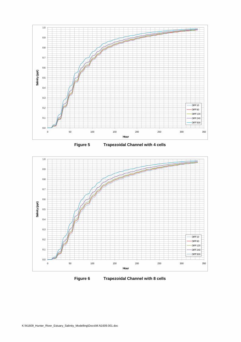
K:\N1609_Hunter_River_Estuary_Salinity_Modelling\Docs\M.N1609.001.doc
0.0
0.1
0.2
0.3
0.4
0.5
0.6
0.7
0.8
0.9
1.0
0 50 100 150 200 250 300 350
Salin
ity
(ppt
)
Hour
DIFF 10
DIFF 60
DIFF 120
DIFF 240
DIFF 500
Figure 5 Trapezoidal Channel with 4 cells
0.0
0.1
0.2
0.3
0.4
0.5
0.6
0.7
0.8
0.9
1.0
0 50 100 150 200 250 300 350
Salin
ity
(ppt
)
Hour
DIFF 10
DIFF 60
DIFF 120
DIFF 240
DIFF 500
Figure 6 Trapezoidal Channel with 8 cells
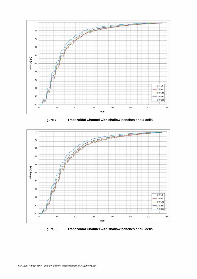
K:\N1609_Hunter_River_Estuary_Salinity_Modelling\Docs\M.N1609.001.doc
0.0
0.1
0.2
0.3
0.4
0.5
0.6
0.7
0.8
0.9
1.0
0 50 100 150 200 250 300 350
Salin
ity
(ppt
)
Hour
DIFF 10
DIFF 60
DIFF 120
DIFF 240
DIFF 500
Figure 7 Trapezoidal Channel with shallow benches and 4 cells
0.0
0.1
0.2
0.3
0.4
0.5
0.6
0.7
0.8
0.9
1.0
0 50 100 150 200 250 300 350
Salin
ity
(ppt
)
Hour
DIFF 10
DIFF 60
DIFF 120
DIFF 240
DIFF 500
Figure 8 Trapezoidal Channel with shallow benches and 8 cells
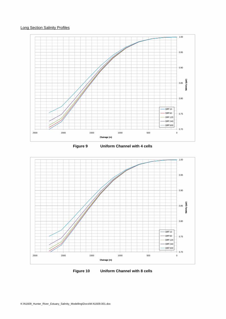
K:\N1609_Hunter_River_Estuary_Salinity_Modelling\Docs\M.N1609.001.doc
Long Section Salinity Profiles
0.70
0.75
0.80
0.85
0.90
0.95
1.00
05001000150020002500
Salin
ity (
ppt)
Chainage (m)
DIFF 10
DIFF 60
DIFF 120
DIFF 240
DIFF 500
Figure 9 Uniform Channel with 4 cells
0.70
0.75
0.80
0.85
0.90
0.95
1.00
05001000150020002500
Salin
ity (
ppt)
Chainage (m)
DIFF 10
DIFF 60
DIFF 120
DIFF 240
DIFF 500
Figure 10 Uniform Channel with 8 cells
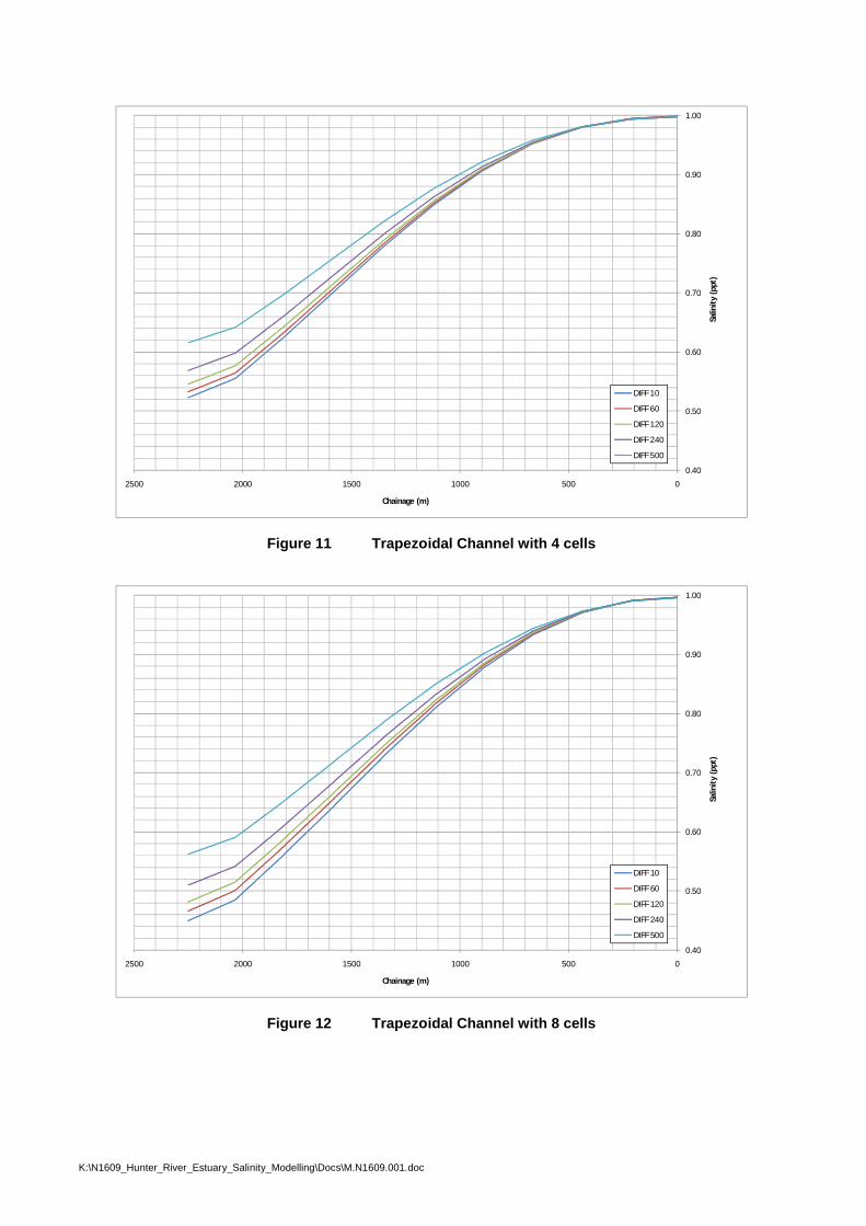
K:\N1609_Hunter_River_Estuary_Salinity_Modelling\Docs\M.N1609.001.doc
0.40
0.50
0.60
0.70
0.80
0.90
1.00
05001000150020002500
Salin
ity (
ppt)
Chainage (m)
DIFF 10
DIFF 60
DIFF 120
DIFF 240
DIFF 500
Figure 11 Trapezoidal Channel with 4 cells
0.40
0.50
0.60
0.70
0.80
0.90
1.00
05001000150020002500
Salin
ity (
ppt)
Chainage (m)
DIFF 10
DIFF 60
DIFF 120
DIFF 240
DIFF 500
Figure 12 Trapezoidal Channel with 8 cells
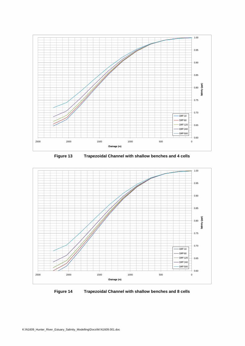
K:\N1609_Hunter_River_Estuary_Salinity_Modelling\Docs\M.N1609.001.doc
0.60
0.65
0.70
0.75
0.80
0.85
0.90
0.95
1.00
05001000150020002500
Salin
ity (
ppt)
Chainage (m)
DIFF 10
DIFF 60
DIFF 120
DIFF 240
DIFF 500
Figure 13 Trapezoidal Channel with shallow benches and 4 cells
0.60
0.65
0.70
0.75
0.80
0.85
0.90
0.95
1.00
05001000150020002500
Salin
ity (
ppt)
Chainage (m)
DIFF 10
DIFF 60
DIFF 120
DIFF 240
DIFF 500
Figure 14 Trapezoidal Channel with shallow benches and 8 cells
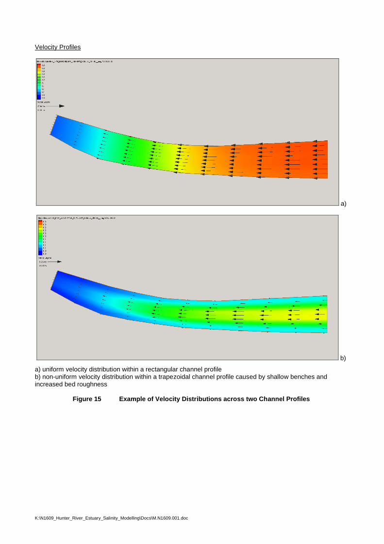
K:\N1609_Hunter_River_Estuary_Salinity_Modelling\Docs\M.N1609.001.doc
Velocity Profiles
a)
b)
a) uniform velocity distribution within a rectangular channel profileb) non-uniform velocity distribution within a trapezoidal channel profile caused by shallow benches and increased bed roughness
Figure 15 Example of Velocity Distributions across two Channel Profiles
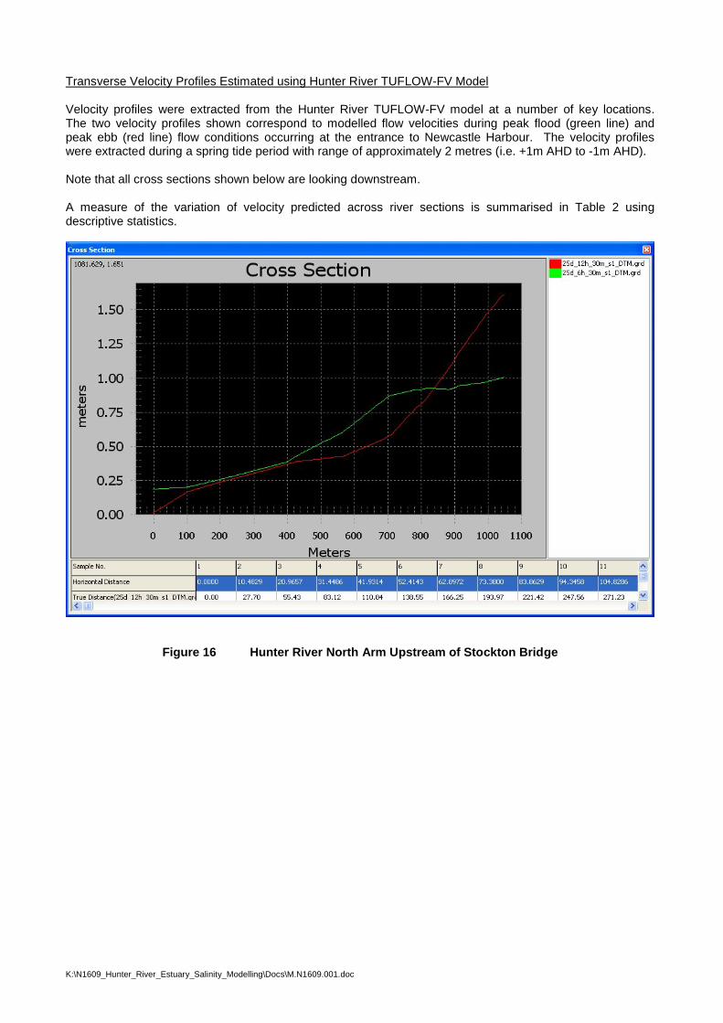
K:\N1609_Hunter_River_Estuary_Salinity_Modelling\Docs\M.N1609.001.doc
Transverse Velocity Profiles Estimated using Hunter River TUFLOW-FV Model
Velocity profiles were extracted from the Hunter River TUFLOW-FV model at a number of key locations. The two velocity profiles shown correspond to modelled flow velocities during peak flood (green line) and peak ebb (red line) flow conditions occurring at the entrance to Newcastle Harbour. The velocity profiles were extracted during a spring tide period with range of approximately 2 metres (i.e. +1m AHD to -1m AHD).
Note that all cross sections shown below are looking downstream.
A measure of the variation of velocity predicted across river sections is summarised in Table 2 using descriptive statistics.
Figure 16 Hunter River North Arm Upstream of Stockton Bridge
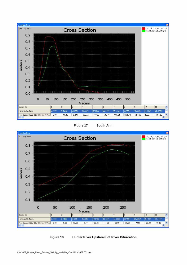
K:\N1609_Hunter_River_Estuary_Salinity_Modelling\Docs\M.N1609.001.doc
Figure 17 South Arm
Figure 18 Hunter River Upstream of River Bifurcation
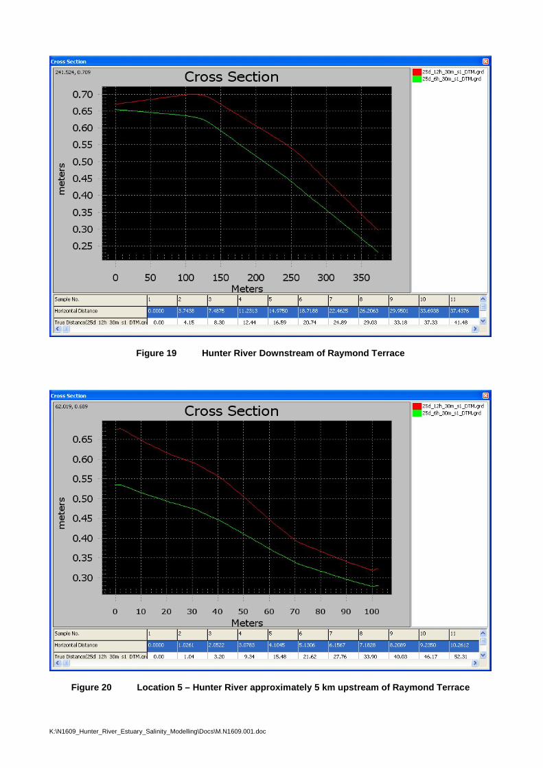
K:\N1609_Hunter_River_Estuary_Salinity_Modelling\Docs\M.N1609.001.doc
Figure 19 Hunter River Downstream of Raymond Terrace
Figure 20 Location 5 – Hunter River approximately 5 km upstream of Raymond Terrace
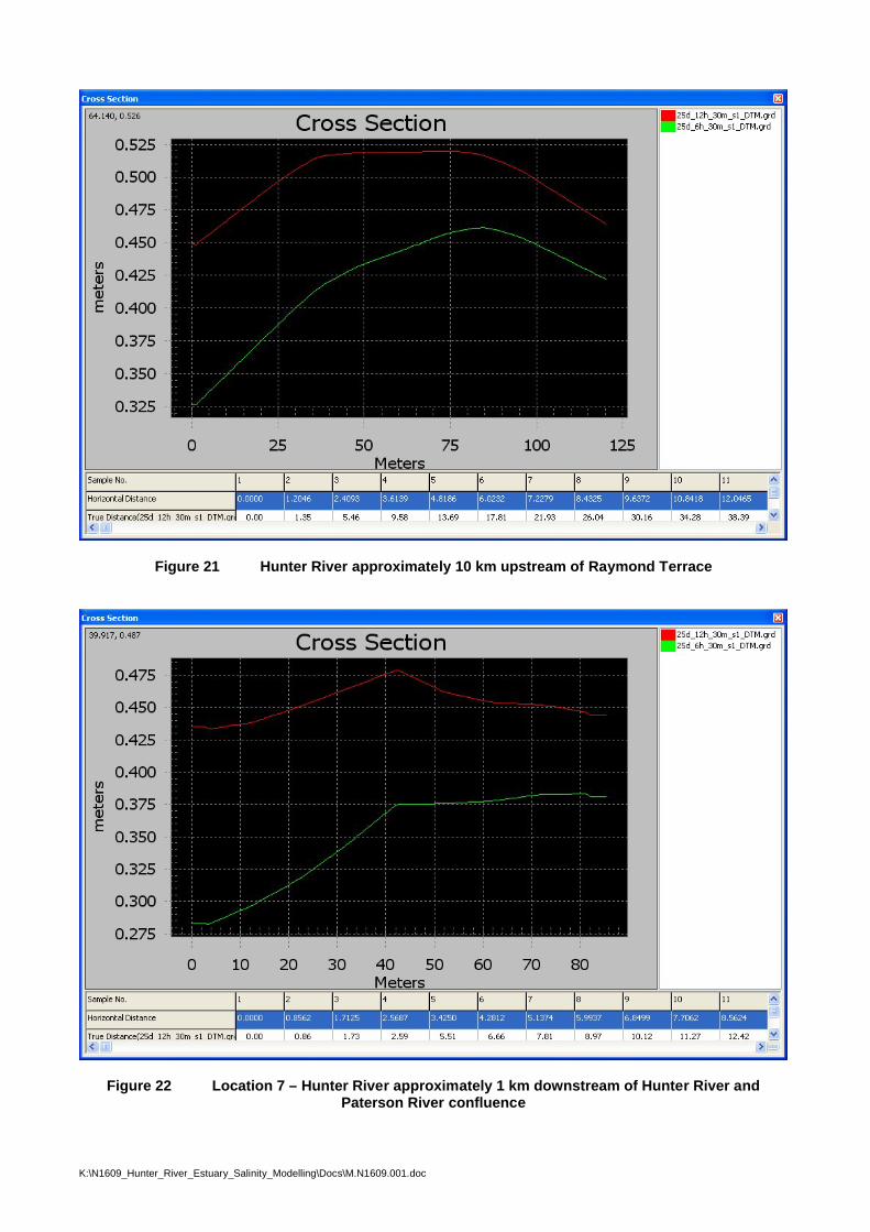
K:\N1609_Hunter_River_Estuary_Salinity_Modelling\Docs\M.N1609.001.doc
Figure 21 Hunter River approximately 10 km upstream of Raymond Terrace
Figure 22 Location 7 – Hunter River approximately 1 km downstream of Hunter River and Paterson River confluence
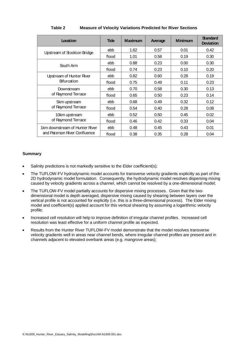
K:\N1609_Hunter_River_Estuary_Salinity_Modelling\Docs\M.N1609.001.doc
Table 2 Measure of Velocity Variations Predicted for River Sections
Location Tide Maximum Average MinimumStandard Deviation
Upstream of Stockton Bridgeebb 1.62 0.57 0.01 0.42
flood 1.01 0.58 0.19 0.30
South Armebb 0.88 0.23 0.00 0.30
flood 0.74 0.23 0.10 0.20
Upstream of Hunter River Bifurcation
ebb 0.82 0.60 0.28 0.19
flood 0.75 0.49 0.11 0.23
Downstreamof Raymond Terrace
ebb 0.70 0.58 0.30 0.13
flood 0.65 0.50 0.23 0.14
5km upstreamof Raymond Terrace
ebb 0.68 0.49 0.32 0.12
flood 0.54 0.40 0.28 0.08
10km upstreamof Raymond Terrace
ebb 0.52 0.50 0.45 0.02
flood 0.46 0.42 0.33 0.04
1km downstream of Hunter River and Paterson River Confluence
ebb 0.48 0.45 0.43 0.01
flood 0.38 0.35 0.28 0.04
Summary
Salinity predictions is not markedly sensitive to the Elder coefficient(s);
The TUFLOW-FV hydrodynamic model accounts for transverse velocity gradients explicitly as part of the 2D hydrodynamic model formulation. Consequently, the hydrodynamic model resolves dispersing mixing caused by velocity gradients across a channel, which cannot be resolved by a one-dimensional model;
The TUFLOW-FV model partially accounts for dispersive mixing processes. Given that the two-dimensional model is depth averaged, dispersive mixing caused by shearing between layers over the vertical profile is not accounted for explicitly (i.e. this is a three-dimensional process). The Elder mixing model and coefficient(s) applied account for this vertical shearing by assuming a logarithmic velocity profile;
Increased cell resolution will help to improve definition of irregular channel profiles. Increased cell resolution was least effective for a uniform channel profile as expected.
Results from the Hunter River TUFLOW-FV model demonstrate that the model resolves transverse velocity gradients well in areas near channel bends, where irregular channel profiles are present and in channels adjacent to elevated overbank areas (e.g. mangrove areas);
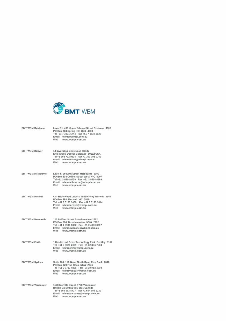
BMT WBM Brisbane Level 11, 490 Upper Edward Street Brisbane 4000PO Box 203 Spring Hill QLD 4004Tel +61 7 3831 6744 Fax +61 7 3832 3627Email [email protected] www.wbmpl.com.au
BMT WBM Denver 14 Inverness Drive East, #B132Englewood Denver Colorado 80112 USATel +1 303 792 9814 Fax +1 303 792 9742Email [email protected] www.wbmpl.com.au
BMT WBM Melbourne Level 5, 99 King Street Melbourne 3000PO Box 604 Collins Street West VIC 8007Tel +61 3 9614 6400 Fax +61 3 9614 6966Email [email protected] www.wbmpl.com.au
BMT WBM Morwell Cnr Hazelwood Drive & Miners Way Morwell 3840PO Box 888 Morwell VIC 3840Tel +61 3 5135 3400 Fax +61 3 5135 3444Email [email protected] www.wbmpl.com.au
BMT WBM Newcastle 126 Belford Street Broadmeadow 2292PO Box 266 Broadmeadow NSW 2292Tel +61 2 4940 8882 Fax +61 2 4940 8887Email [email protected] www.wbmpl.com.au
BMT WBM Perth 1 Brodie Hall Drive Technology Park Bentley 6102Tel +61 8 9328 2029 Fax +61 8 9486 7588Email [email protected] www.wbmpl.com.au
BMT WBM Sydney Suite 206, 118 Great North Road Five Dock 2046PO Box 129 Five Dock NSW 2046Tel +61 2 9713 4836 Fax +61 2 9713 4890Email [email protected] www.wbmpl.com.au
BMT WBM Vancouver 1190 Melville Street #700 VancouverBritish Columbia V6E 3W1 CanadaTel +1 604 683 5777 Fax +1 604 608 3232Email [email protected] www.wbmpl.com.au


![Monitoring and Evaluation Report Colorado River Salinity Control … · [1] Monitoring and Evaluation Report Colorado River Salinity Control Units Lower Gunnison, McElmo Creek, Mancos](https://img.pdfslide.us/doc/110x75/5f8ffe97a577d44070077650/monitoring-and-evaluation-report-colorado-river-salinity-control-1-monitoring.jpg)