Assessment of OpenFOAM CFD Toolbox for Gravity driven …glc.ans.org/nureth-16/data/papers/13200.pdf · 2015-08-12 · ASSESSMENT OF OPENFOAM CFD TOOLBOX FOR GRAVITY DRIVEN MIXING

ASSESSMENT OF OPENFOAM CFD TOOLBOX FOR GRAVITY DRIVEN MIXING FLOWS IN A REACTOR PRESSURE VESSEL

R. Puragliesi∗∗, O. Zerkak and A. Pautz Laboratory for Reactor Physics and Systems Behavior

Paul Scherrer Institute, CH-5232 Villigen PSI, Switzerland [email protected]; [email protected]; [email protected]

Q. Zhou Laboratoire des Applications en Thermohydraulique et Mécanique des Fluides

CEA Saclay, 91191 Gif-sur-Yvette Cedex, France [email protected]

ABSTRACT

An assessment of the open-source CFD software package OpenFOAM has been performed considering buoyancy-driven mixing flow inside a KONVOI type Reactor Pressure Vessel (RPV). The intrinsic complexity of the geometry and the physics of the flow are beyond the reach of one-dimensional thermal-hydraulic system codes, and thus the need to use properly verified and validated CFD simulation tools and models originates. The chosen test represents a typical configuration that occurs during a Main Steam Line Break (MSLB) with Loss-Of-Offsite-Power (LOOP) scenario. The experiment Test 1.1 of the ROssendorf COolant Mixing (ROCOM) facility has been selected from the OECD-NEA PKL-2 project database. Previous analysis showed that Unsteady Reynolds Averaged Navier-Stokes (URANS) solutions are strongly affected by the physical and turbulent transport properties. A hexahedral mesh was employed to discretize all the geometrical details important for the mixing process in the RPV. To evaluate the accuracy of the code, a modified transient, incompressible solver was developed to include a variable turbulent Prandtl number formulation to resemble as closely as possible to the best performing numerical model previously identified using the commercial code STAR-CCM+. The paper presents the first attempt to model the mixing in a RPV during a MSLB LOOP scenario with the open-source code OpenFOAM. Results indicate that the modified solver is usable for gravity driven flows but the current model needs improvements, in particular the mesh generation. It was also confirmed that a large integration time-step leads to a wrong estimation of the mixing, especially in the downcomer region.

KEYWORDS Turbulent mixing, CFD URANS, ROCOM, gravity driven flow, OpenFOAM

1. INTRODUCTION

Non-uniform distribution of coolant temperature, or moderator concentration, at the core-inlet of a pressurized water reactor vessel, can be caused by asymmetrical inlet flow conditions. Indeed, the hypothesis of perfect mixing has been shown to be not conservative [1] since the crucial safety limits (e.g.

∗ Corresponding author.

952NURETH-16, Chicago, IL, August 30-September 4, 2015 952NURETH-16, Chicago, IL, August 30-September 4, 2015

return to criticality of the core or local thermal stresses in the RPV) are intrinsically related to the time-evolution of the mixing inside the RPV. Two important facts occurring during a MSLB+LOOP, i.e. the early trip of the main coolant recirculation pumps and the concomitant high temperature differences between the loops, lead to buoyancy driven mixing flows. This type of flows is increasingly studied, both from the experimental and the numerical viewpoints: A non-exhaustive list of publications on the validation of CFD codes against ROCOM experiments is provided [2-8]. It can be noticed that most of the CFD studies, published so far, based on ROCOM MSLB tests, show a higher vertical position of the transition line of the mixing scalar (i.e. where a clear separation between light/hot and heavy/cold coolant occurs because of incomplete mixing and stratification) in comparison with the experiment. Moreover, this behavior was found to be rather insensitive to changes in parameters like mesh (block structured or hybrid), grid-size in a certain measure, turbulent models, slug injection position, fillet of the inlet nozzles. Recently in [9] it was found that the mixing dynamics in the downcomer is very sensible to the physical and turbulent parameters that describe the momentum and active scalar diffusivity. For the present study, a first attempt to explicitly model the geometry of a KONVOI type RPV, with the open-source code OpenFOAM, is presented. The CFD model is also assessed using the available experimental data collected at the ROCOM test facility as part of the OECD-NEA PKL 2 Project: Test 1.1, with quasi-steady flow conditions and high density ratio between the coolant coming from the affected loop (cold leg 1, CL1), and that injected from the other loops (cold leg 2, 3 and 4, CL2-4), was chosen. Following the same rationale of [9], the transport of the mixing scalar is based on an equivalent thermal model of the experimental system. In particular a correction of the molecular Prandtl number was introduced as well as the implementation of an ad-hoc variable turbulent Prandtl number optimized for buoyant flows [10]. The paper is organized as follows: In Section 2 the experimental facility is briefly described�� numerical setup together with the approach used to model the physical properties and the turbulent Prandtl number are given �� is devoted to results and discussion�� tion 5, conclusions and future developments are given.

2. ROCOM FACILITY

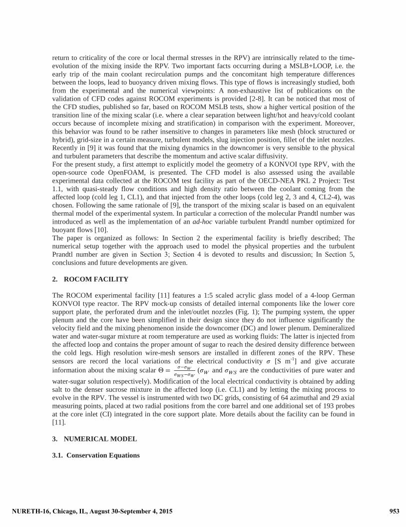
The ROCOM experimental facility [11] features a 1:5 scaled acrylic glass model of a 4-loop German KONVOI type reactor. The RPV mock-up consists of detailed internal components like the lower core support plate, the perforated drum and the inlet/outlet nozzles (Fig. 1); The pumping system, the upper plenum and the core have been simplified in their design since they do not influence significantly the velocity field and the mixing phenomenon inside the downcomer (DC) and lower plenum. Demineralized water and water-sugar mixture at room temperature are used as working fluids: The latter is injected from the affected loop and contains the proper amount of sugar to reach the desired density difference between the cold legs. High resolution wire-mesh sensors are installed in different zones of the RPV. These sensors are record the local variations of the electrical conductivity 𝜎 [S m-1] and give accurate information about the mixing scalar Θ = 𝜎−𝜎𝑊

𝜎𝑊𝑆−𝜎𝑊 (𝜎𝑊 and 𝜎𝑊𝑆 are the conductivities of pure water and

water-sugar solution respectively). Modification of the local electrical conductivity is obtained by adding salt to the denser sucrose mixture in the affected loop (i.e. CL1) and by letting the mixing process to evolve in the RPV. The vessel is instrumented with two DC grids, consisting of 64 azimuthal and 29 axial measuring points, placed at two radial positions from the core barrel and one additional set of 193 probes at the core inlet (CI) integrated in the core support plate. More details about the facility can be found in [11].

3. NUMERICAL MODEL

3.1. Conservation Equations


In the following, the SI units system is employed. The governing equations in vector notation for a transient, incompressible, viscous Newtonian, turbulent flow written in the RANS framework read

Figure 1 Schematic of ROCOM RPV internals.

𝛁 ⋅ 𝐮 = 0, (1)

𝜕𝐮𝜕𝑡

+ 𝛁 ⋅ (𝐮 𝐮) = −𝛁𝑝 + 𝛁 ⋅ (2𝜈𝐒 + 𝐓𝑡) + 𝐟𝐵 � (2)

𝜕𝑇𝜕𝑡

+ 𝛁 ⋅ (𝑇 𝐮) = 𝛁 ⋅ (𝜈𝑃𝑟

𝛁𝑇 + 𝐪𝑡), (3)

with 𝐮 the average velocity field, 𝑡 the time, 𝑝 = 𝑃𝜌 the average pressure field (� being the actual static

pressure), � the kinematic viscosity, 𝐒 the symmetric part of the gradient of the average velocity field, 𝐓𝑡the Reynolds stress tensor, 𝐟𝐵 the average specific buoyancy force, 𝑇 the average temperature field. The molecular Prandtl number is indicated with 𝑃𝑟 = 𝜈/𝛼 (𝜈 and 𝛼 being the molecular kinematic viscosity and molecular thermal diffusivity) while the turbulent heat flux is 𝐪𝑡. Finally, the symbol 𝛁 is employed for the gradient operator. The Boussinesq approximation [12, 13] was chosen for modelling the buoyancy term in Eq. (3), i.e.

𝐟𝐵 = 𝐠𝛽(𝑇𝑅𝐸𝐹 − 𝑇 )� (4)where the gravity acceleration vector 𝐠 appears, the volumetric expansion coefficient is indicated with 𝛽and 𝑇𝑅𝐸𝐹 is the reference temperature. A two-equation turbulence model based on the standard 𝑘 − 𝜖 is used to relate the turbulent scales to the Reynolds stress tensor. The well-known Boussinesq eddy-viscosity hypothesis is employed,

𝐓𝑡 = 2𝜈𝑡𝐒� �� (5)

where the turbulent kinematic viscosity is defined as

𝜈𝑡 = 𝐶𝜇𝑘2

𝜖 (6)

The transport equations for the turbulent kinetic energy ��and its dissipation rate 𝜖, contain the additional terms due to the work of the gravitational field [14]

𝜕𝑘𝜕𝑡

+ 𝛁 ⋅ (𝑘 𝐮) = 𝛁 ⋅ [(𝜈 +𝜈𝑇 𝜎𝑘 ) 𝛁𝑘] + (𝐺𝑘 + 𝐵𝑘 − 𝜖), (7)

𝜕𝜖𝜕𝑡

+ 𝛁 ⋅ (𝜖 𝐮) = 𝛁 ⋅ [(𝜈 +𝜈𝑇 𝜎𝜖 ) 𝛁𝜖] + 𝜖

𝑘 [𝐶𝜖1𝐺𝑘 + 𝐶𝜖3𝐵𝜖 − 𝐶𝜖2𝜖]� (8)


where the model coefficients take the following values

𝜎𝑘 = 1.0, 𝜎𝜖 = 1.3, 𝐶𝜖1 = 1.44, 𝐶𝜖2 = 1.92, 𝐶𝜖3 = 1.44 (9)The additional source/sink terms depend on the average flow field

𝐺𝑘 = 2𝜈𝑡|𝐒|2� �� (� � ��)� ��

� �� . (10)

The problem is finally closed by using the Boussinesq eddy-diffusivity approach in order to model the turbulent heat flux in Eq. (3), i.e.

𝐪𝑡 = �� , (11)

which requires the CFD analyst to provide the turbulent Prandtl number �� 𝜈𝑡/𝛼𝑡 (𝛼𝑡 being the turbulent thermal diffusivity) as model parameter.

3.1.1. Turbulent Prandtl number

The standard approach is to use a constant field with a turbulent Prandtl number in the range 0.7 ≤ 𝑃𝑟𝑡 ≤1 which is commonly adopted for turbulent water flows [15]. As pinpointed in [9], for our particular application, the mixing dynamics in the downcomer can be improved by using a variable turbulent Prandtl number suited for flows characterized by stable density stratification. The idea behind is to include a dependency on the local ratio of the turbulent frequency (inverse of the turbulent time-scale) and the

Brunt-Väisälä frequency � �� ! "�# [10] which characterizes internal gravity waves. Following [9,

10] a generalized formulation is adopted

{𝑃𝑟𝑡 = 1.0 if gg⋅∇T $ 0𝑃𝑟𝑡 = 1.0 + 0.4 exp(−2.5 𝐹𝑟𝑡) if gg⋅∇T % 0 (12)

with the local turbulent Froude number defined as 𝐹𝑟𝑡 = ��. From theory, in a stably stratified

environment, the stability of the flow increases with increasing � (i.e. more energy is required to perturb the system), leading to a decrease of the mixing process in those regions with high density gradients. With Eq. (12) the decrease of mixing is actually achieved by high values of the turbulent Prandtl number (𝑃𝑟𝑡 ≈1.4) whereas in regions of unstable stratification or homogenous density field, the turbulent Prandtl number tends to 1.

3.1.2. Physical properties modelling

The test specifications require performing an initialization phase followed by the actual natural circulation and mixing phase. For the former, demineralized water with constant standard properties is injected from CL2-4 (no flow in CL1), whereas a mixture of water and sugar is injected from the affected loop CL1 in the latter (more details will be given in Sec. 3.2.1). For the natural circulation and mixing phase the physical properties are prescribed to mimic the actual isothermal experimental system. The constant product 𝛽(𝑇𝐶𝐿24 − 𝑇𝐶𝐿1) is set according to the coolant density difference (i.e. 12%) between the affected loop CL1 and the non-affected loops CL2-4. The actual dynamic viscosity and the molecular diffusivity of the water-sugar mixture were not provided in the technical documentation and/or published literature of the selected test. In Fig. 2 the variation of density ratio and kinematic viscosity ratio as function of sugar concentration in water solution are shown. It must be noticed that the molecular diffusivity of sugar in water (~10-9 [m2 s-1]) [6, 7] is two orders of magnitude lower than the thermal diffusivity of water at


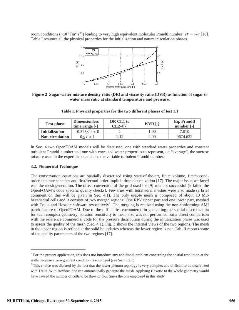
room conditions (~10-7 [m2 s-1]) leading to very high equivalent molecular Prandtl number1 𝑃𝑟 = 𝜈/𝛼 [16]. Table I resumes all the physical properties for the initialization and natural circulation phases.

Figure 2 Sugar-water mixture density ratio (DR) and viscosity ratio (DVR) as function of sugar to water mass ratio at standard temperature and pressure.

Table I. Physical properties for the two different phases of test 1.1

Test phase Dimensionless time range [-]

DR CL1 to CL2-4[-] KVR [-] Eq. Prandtl

number [-] Initialization -0.375≤ 𝑡 ̃ < 0 1 1.00 7.010 Nat. circulation 0≤ 𝑡 ̃ < 1 1.12 2.00 9674.622

In Sec. 4 two OpenFOAM models will be discussed, one with standard water properties and constant turbulent Prandtl number and one with corrected water properties to represent, on “average”, the sucrose mixture used in the experiments and also the variable turbulent Prandtl number.

3.2. Numerical Technique

The conservation equations are spatially discretized using state-of-the-art, finite volume, first/second-order accurate schemes and first/second-order implicit time discretization [17]. The major issue we faced was the mesh generation. The direct conversion of the grid used for [9] was not successful (it failed the OpenFOAM’s code specific quality checks). Few tries with tetrahedral meshes were also made (a brief comment on this will be given in Sec. 4.1). The only usable mesh is composed of about 13 Mio hexahedral cells and it consists of two merged regions: One RPV upper part and one lower part, meshed with Trelis and Hexotic software respectively2. The merging is realized using the non-conforming AMI patch feature of OpenFOAM. Due to the difficulties encountered in generating the spatial discretization for such complex geometry, solution sensitivity to mesh size was not performed but a direct comparison with the reference commercial code for the pressure distribution during the initialization phase was used to assess the quality of the mesh (Sec. 4.1). Fig. 3 shows the internal views of the two regions. The mesh in the upper region is refined at the solid boundaries whereas the lower region is not. Tab. II reports some of the quality parameters of the two regions [17].

1 For the present application, this does not introduce any additional problem concerning the spatial resolution at the walls because a zero gradient condition is employed (see Sec. 3.2.1). 2 This choice was dictated by the fact that the lower plenum topology is very complex and difficult to be discretized

with Trelis. With Hexotic, one can automatically generate the mesh. Applying Hexotic to the whole geometry would have caused the number of cells to be three or four times the one employed in this study.


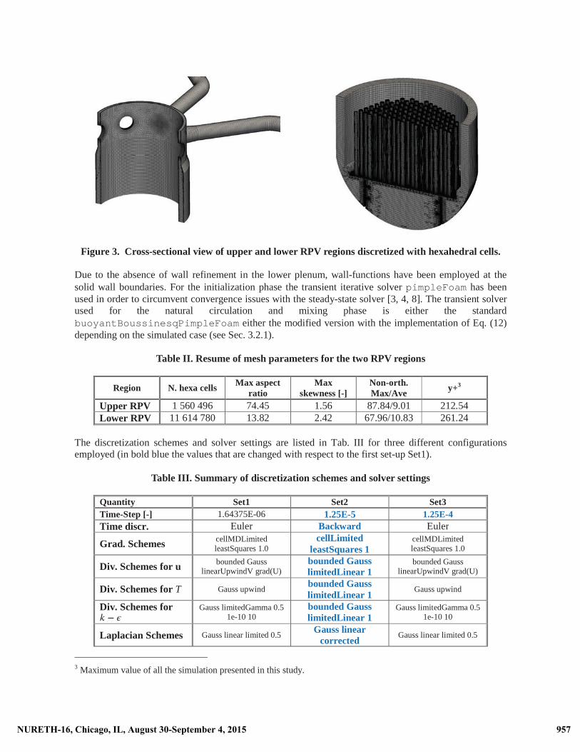
Figure 3. Cross-sectional view of upper and lower RPV regions discretized with hexahedral cells.

Due to the absence of wall refinement in the lower plenum, wall-functions have been employed at the solid wall boundaries. For the initialization phase the transient iterative solver pimpleFoam has been used in order to circumvent convergence issues with the steady-state solver [3, 4, 8]. The transient solver used for the natural circulation and mixing phase is either the standard buoyantBoussinesqPimpleFoam either the modified version with the implementation of Eq. (12) depending on the simulated case (see Sec. 3.2.1).

Table II. Resume of mesh parameters for the two RPV regions

Region N. hexa cells Max aspect ratio

Max skewness [-]

Non-orth. Max/Ave y+3

Upper RPV 1 560 496 74.45 1.56 87.84/9.01 212.54Lower RPV 11 614 780 13.82 2.42 67.96/10.83 261.24

The discretization schemes and solver settings are listed in Tab. III for three different configurations employed (in bold blue the values that are changed with respect to the first set-up Set1).

Table III. Summary of discretization schemes and solver settings

Quantity Set1 Set2 Set3 Time-Step [-] 1.64375E-06 1.25E-5 1.25E-4Time discr. Euler Backward Euler

Grad. Schemes cellMDLimited leastSquares 1.0

cellLimited leastSquares 1

cellMDLimited leastSquares 1.0

Div. Schemes for u bounded Gauss linearUpwindV grad(U)

bounded Gauss limitedLinear 1

bounded Gauss linearUpwindV grad(U)

Div. Schemes for T Gauss upwindbounded Gauss limitedLinear 1 Gauss upwind

Div. Schemes for 𝑘 − 𝜖

Gauss limitedGamma 0.5 1e-10 10

bounded Gauss limitedLinear 1

Gauss limitedGamma 0.5 1e-10 10

Laplacian Schemes Gauss linear limited 0.5Gauss linear

corrected Gauss linear limited 0.5

3 Maximum value of all the simulation presented in this study.


Under-relax. factor for u

0.5 0.8 0.5

Under-relax. factor for p 0.3 0.5 0.3

Under-relax. factor for T 0.7 0.8 0.7

Under-relax. factor𝑘 − 𝜖 0.5 0.8 0.5

Solver for u Smoother GaussSeidel

Smoother GaussSeidel


Solver for p GAMG GAMG GAMG

Solver for T Smoother GaussSeidel



Solver for 𝑘 − 𝜖 Smoother GaussSeidel



For more details of some specific discretization/solver options refer to [17].

3.2.1. Initial and boundary conditions

In the next section, four OpenFOAM simulations will be compared together with two reference simulations performed with a commercial code [18] and experimental measurements in order to understand the influence of the time-step in the solutions. In table IV the different combinations of solver settings and physical parameters are provided.

Table IV. Simulation list

Sim. Phys. prop. 𝑃𝑟𝑡

Sol. settings

OF1 Standard 0.9 Set3OF2 Standard 0.9 Set2OF3 Corrected Eq. (12) Set3OF4 Corrected Eq. (12) Set1

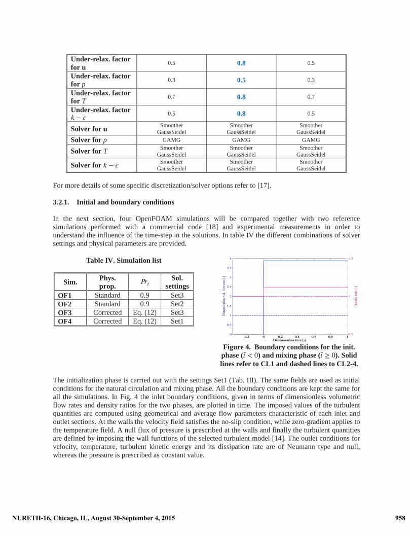
Figure 4. Boundary conditions for the init. phase (𝑡 ̃ < 0) and mixing phase (𝑡 ̃ ≥ 0). Solid lines refer to CL1 and dashed lines to CL2-4.

The initialization phase is carried out with the settings Set1 (Tab. III). The same fields are used as initial conditions for the natural circulation and mixing phase. All the boundary conditions are kept the same for all the simulations. In Fig. 4 the inlet boundary conditions, given in terms of dimensionless volumetric flow rates and density ratios for the two phases, are plotted in time. The imposed values of the turbulent quantities are computed using geometrical and average flow parameters characteristic of each inlet and outlet sections. At the walls the velocity field satisfies the no-slip condition, while zero-gradient applies to the temperature field. A null flux of pressure is prescribed at the walls and finally the turbulent quantities are defined by imposing the wall functions of the selected turbulent model [14]. The outlet conditions for velocity, temperature, turbulent kinetic energy and its dissipation rate are of Neumann type and null,whereas the pressure is prescribed as constant value.


4. RESULTS AND DISCUSSION

In the present section results are given in terms of dimensionless temperature which is a quantity derived from the definition of mixing scalar via the simple relationship 𝑇̃ = 1 − Θ. For a general scalar field 𝜙(𝑥, 𝑦, 𝑧, 𝑡), the space-averaging operator ⟨𝜙⟩(𝑡) is defined as the expected value of the spatial distribution at instant 𝑡. The spatial coordinates shown in the maps correspond to the indices of the probes in a matrix configuration. Moreover the probe layouts have been kept consistent to the original configuration of the experiment setup.

4.1. Initialization Phase

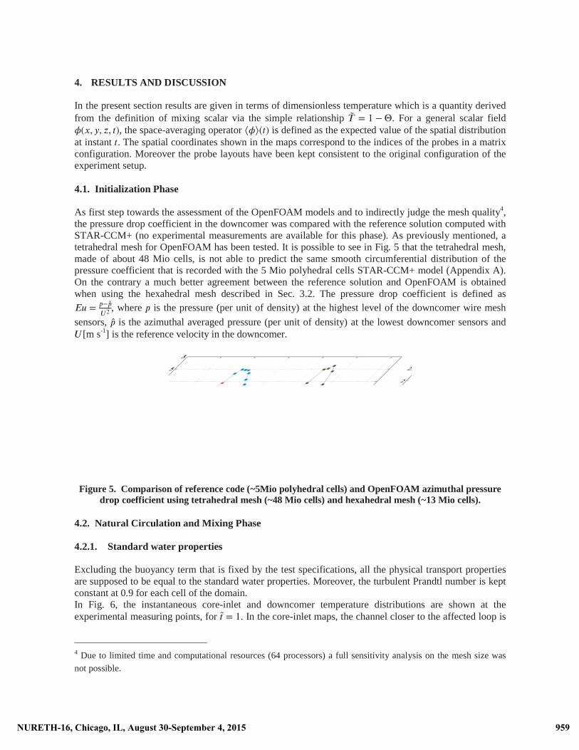
As first step towards the assessment of the OpenFOAM models and to indirectly judge the mesh quality4, the pressure drop coefficient in the downcomer was compared with the reference solution computed with STAR-CCM+ (no experimental measurements are available for this phase). As previously mentioned, a tetrahedral mesh for OpenFOAM has been tested. It is possible to see in Fig. 5 that the tetrahedral mesh, made of about 48 Mio cells, is not able to predict the same smooth circumferential distribution of the pressure coefficient that is recorded with the 5 Mio polyhedral cells STAR-CCM+ model (Appendix A). On the contrary a much better agreement between the reference solution and OpenFOAM is obtained when using the hexahedral mesh described in Sec. 3.2. The pressure drop coefficient is defined as 𝐸𝑢 = 𝑝−𝑝̂

𝑈2 , where 𝑝 is the pressure (per unit of density) at the highest level of the downcomer wire mesh

sensors, 𝑝 ̂ is the azimuthal averaged pressure (per unit of density) at the lowest downcomer sensors and 𝑈 [m s-1] is the reference velocity in the downcomer.

Figure 5. Comparison of reference code (~5Mio polyhedral cells) and OpenFOAM azimuthal pressure drop coefficient using tetrahedral mesh (~48 Mio cells) and hexahedral mesh (~13 Mio cells).

4.2. Natural Circulation and Mixing Phase

4.2.1. Standard water properties

Excluding the buoyancy term that is fixed by the test specifications, all the physical transport properties are supposed to be equal to the standard water properties. Moreover, the turbulent Prandtl number is kept constant at 0.9 for each cell of the domain. In Fig. 6, the instantaneous core-inlet and downcomer temperature distributions are shown at the experimental measuring points, for 𝑡 ̃ = 1. In the core-inlet maps, the channel closer to the affected loop is

4 Due to limited time and computational resources (64 processors) a full sensitivity analysis on the mesh size was not possible.


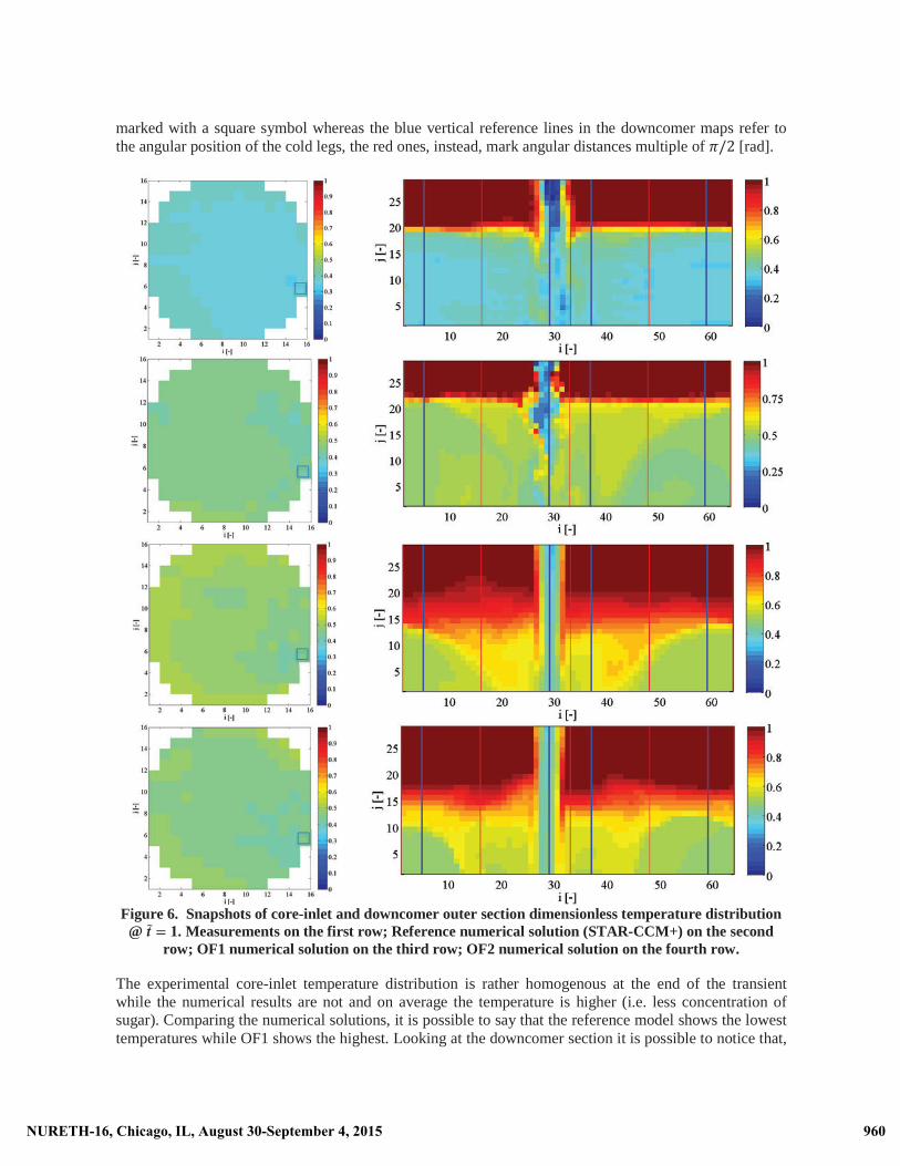
marked with a square symbol whereas the blue vertical reference lines in the downcomer maps refer to the angular position of the cold legs, the red ones, instead, mark angular distances multiple of &'� [rad].

Figure 6. Snapshots of core-inlet and downcomer outer section dimensionless temperature distribution @ 𝒕 ̃ = 𝟏. Measurements on the first row; Reference numerical solution (STAR-CCM+) on the second

row; OF1 numerical solution on the third row; OF2 numerical solution on the fourth row.

The experimental core-inlet temperature distribution is rather homogenous at the end of the transient while the numerical results are not and on average the temperature is higher (i.e. less concentration of sugar). Comparing the numerical solutions, it is possible to say that the reference model shows the lowest temperatures while OF1 shows the highest. Looking at the downcomer section it is possible to notice that,


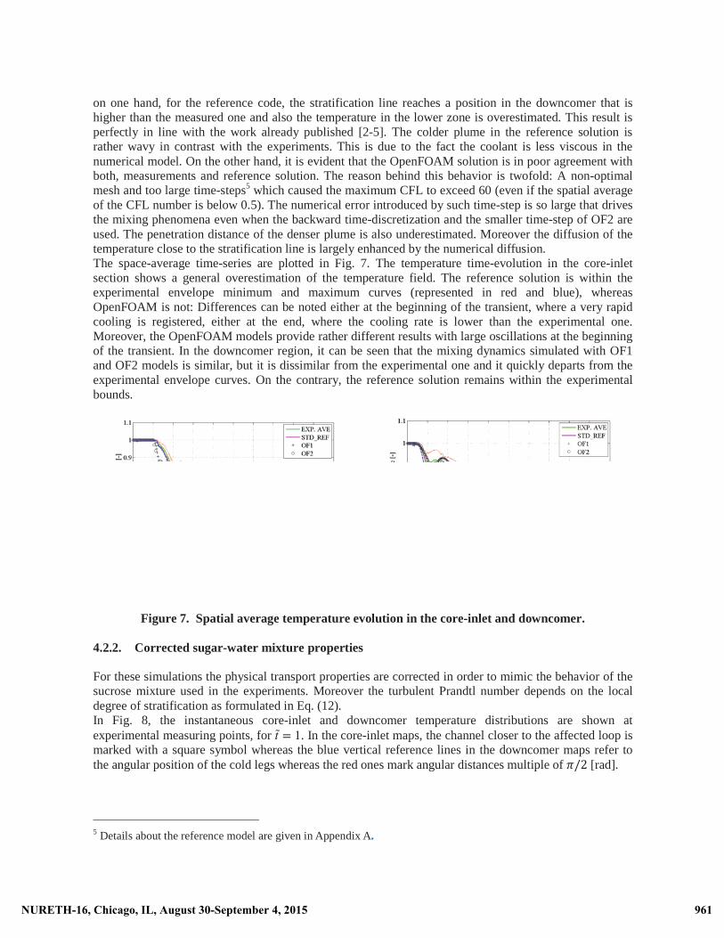
on one hand, for the reference code, the stratification line reaches a position in the downcomer that is higher than the measured one and also the temperature in the lower zone is overestimated. This result is perfectly in line with the work already published [2-5]. The colder plume in the reference solution is rather wavy in contrast with the experiments. This is due to the fact the coolant is less viscous in the numerical model. On the other hand, it is evident that the OpenFOAM solution is in poor agreement with both, measurements and reference solution. The reason behind this behavior is twofold: A non-optimal mesh and too large time-steps5 which caused the maximum CFL to exceed 60 (even if the spatial average of the CFL number is below 0.5). The numerical error introduced by such time-step is so large that drives the mixing phenomena even when the backward time-discretization and the smaller time-step of OF2 are used. The penetration distance of the denser plume is also underestimated. Moreover the diffusion of the temperature close to the stratification line is largely enhanced by the numerical diffusion. The space-average time-series are plotted in Fig. 7. The temperature time-evolution in the core-inlet section shows a general overestimation of the temperature field. The reference solution is within the experimental envelope minimum and maximum curves (represented in red and blue), whereas OpenFOAM is not: Differences can be noted either at the beginning of the transient, where a very rapid cooling is registered, either at the end, where the cooling rate is lower than the experimental one. Moreover, the OpenFOAM models provide rather different results with large oscillations at the beginning of the transient. In the downcomer region, it can be seen that the mixing dynamics simulated with OF1 and OF2 models is similar, but it is dissimilar from the experimental one and it quickly departs from the experimental envelope curves. On the contrary, the reference solution remains within the experimental bounds.

Figure 7. Spatial average temperature evolution in the core-inlet and downcomer.

4.2.2. Corrected sugar-water mixture properties

For these simulations the physical transport properties are corrected in order to mimic the behavior of the sucrose mixture used in the experiments. Moreover the turbulent Prandtl number depends on the local degree of stratification as formulated in Eq. (12).In Fig. 8, the instantaneous core-inlet and downcomer temperature distributions are shown at experimental measuring points, for 𝑡 ̃ = 1. In the core-inlet maps, the channel closer to the affected loop is marked with a square symbol whereas the blue vertical reference lines in the downcomer maps refer to the angular position of the cold legs whereas the red ones mark angular distances multiple of &'� [rad].

5 Details about the reference model are given in Appendix A.


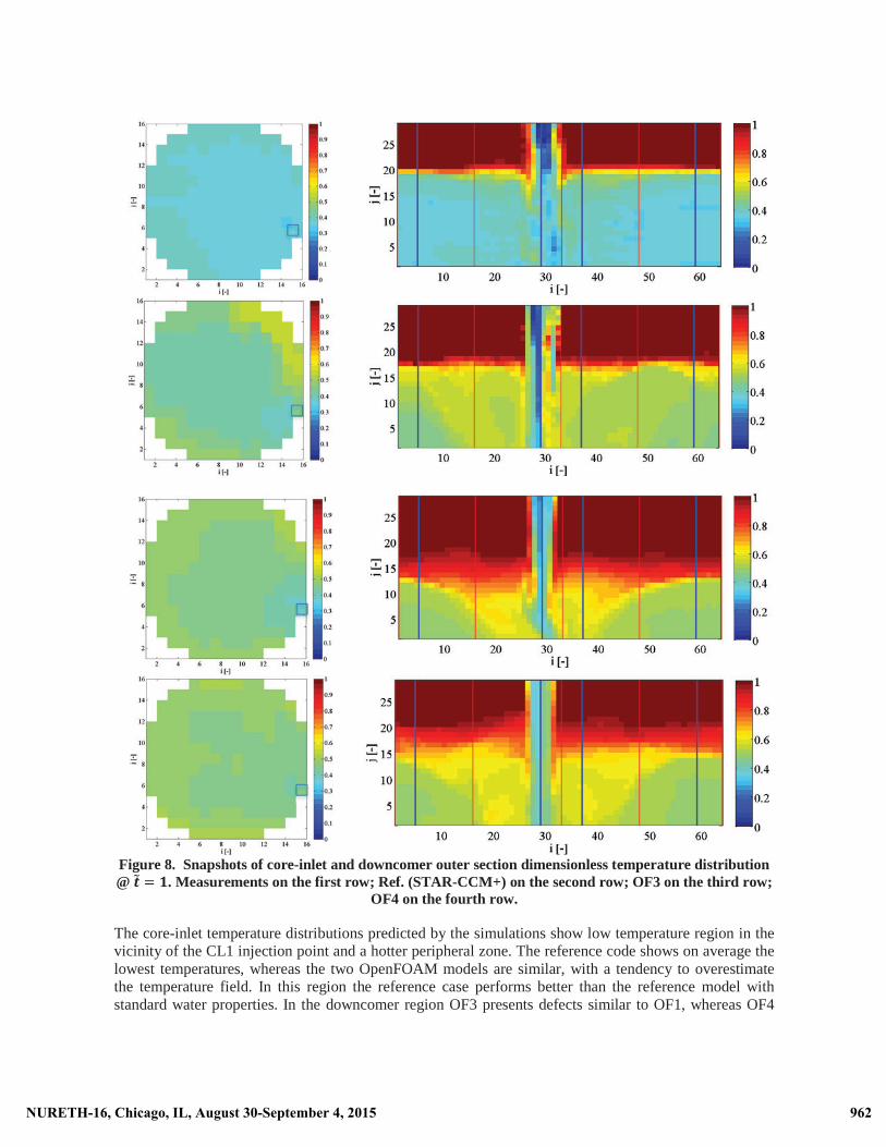
Figure 8. Snapshots of core-inlet and downcomer outer section dimensionless temperature distribution @ () *. Measurements on the first row; Ref. (STAR-CCM+) on the second row; OF3 on the third row;

OF4 on the fourth row.

The core-inlet temperature distributions predicted by the simulations show low temperature region in the vicinity of the CL1 injection point and a hotter peripheral zone. The reference code shows on average the lowest temperatures, whereas the two OpenFOAM models are similar, with a tendency to overestimate the temperature field. In this region the reference case performs better than the reference model with standard water properties. In the downcomer region OF3 presents defects similar to OF1, whereas OF4


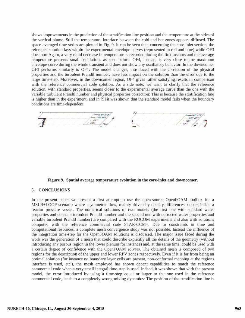
shows improvements in the prediction of the stratification line position and the temperature at the sides of the vertical plume. Still the temperature interface between the cold and hot zones appears diffused. The space-averaged time-series are plotted in Fig. 9. It can be seen that, concerning the core-inlet section, the reference solution lays within the experimental envelope curves (represented in red and blue) while OF3 does not: Again, a very rapid decrease in temperature is recorded during the first instants and the average temperature presents small oscillations as seen before. OF4, instead, is very close to the maximum envelope curve during the whole transient and does not show any oscillatory behavior. In the downcomerOF3 performs similarly to OF1: The model changes, introduced with the correction of the physical properties and the turbulent Prandtl number, have less impact on the solution than the error due to the large time-step. Moreover, in the downcomer region, OF4 gives rather satisfying results in comparison with the reference commercial code solution. As a side note, we want to clarify that the reference solution, with standard properties, seems closer to the experimental average curve than the one with the variable turbulent Prandtl number and physical properties correction: This is because the stratification line is higher than in the experiment, and in [9] it was shown that the standard model fails when the boundary conditions are time-dependent.

Figure 9. Spatial average temperature evolution in the core-inlet and downcomer.

5. CONCLUSIONS

In the present paper we present a first attempt to use the open-source OpenFOAM toolbox for a MSLB+LOOP scenario where asymmetric flow, mainly driven by density differences, occurs inside a reactor pressure vessel. The numerical solutions of two models (the first one with standard water properties and constant turbulent Prandtl number and the second one with corrected water properties and variable turbulent Prandtl number) are compared with the ROCOM experiments and also with solutions computed with the reference commercial code STAR-CCM+. Due to constraints in time and computational resources, a complete mesh convergence study was not possible. Instead the influence of the integration time-step for the OpenFOAM solutions is discussed. The major issue faced during the work was the generation of a mesh that could describe explicitly all the details of the geometry (without introducing any porous region in the lower plenum for instance) and, at the same time, could be used with a certain degree of confidence with the OpenFOAM solvers. The obtained mesh is composed of two regions for the description of the upper and lower RPV zones respectively. Even if it is far from being an optimal solution (for instance no boundary layer cells are present, non-conformal mapping at the regions interface is used, etc.), the mesh employed has shown decent capabilities to match the reference commercial code when a very small integral time-step is used. Indeed, it was shown that with the present model, the error introduced by using a time-step equal or larger to the one used in the reference commercial code, leads to a completely wrong mixing dynamics: The position of the stratification line is


largely underestimated, while the temperature is overestimated. In general it can be concluded that the present OpenFOAM model is more diffusive than the commercial one even if the results obtained using very small time-step, corrected physical properties and variable turbulent Prandtl number, look encouraging. In the future, efforts will be focused in generating a more appropriate mesh that includes boundary layer refinement and also a more general treatment of variable properties (non-linear dependency on the concentration field, for instance) will be implemented in the standard solver for two-liquid components.

ACKNOWLEDGMENTS

This work was partly funded by the Swiss Federal Nuclear Safety Inspectorate ENSI (Eidgenössisches Nuklearsicherheitsinspektorat), within the framework of the STARS project (http://stars.web.psi.ch). The authors are also grateful to the Management Board of the OECD-NEA PKL 2 project for providing the opportunity to publish the results and to the Helmholtz-Zentrum Dresden-Rossendorf for access to the ROCOM data.

REFERENCES

1. R.W. Lyczkowski, J.H. Kim, H.P. Fol, "Analysis of a PWR downcomer and lower plenum under asymmetric loop flow conditions," Proceeding of American Nuclear Society-Annual Meeting, Boston, Massachusetts, June 9-14 (1985).

2. A. Barthet, B. Gaudron, D. Alvarez, “CODE_SATURNE integral validation on a ROCOM test,” Proceeding of Int. Top. Meetg. Nuclear Reactor Thermalhydraulics, NURETH-15, Pisa, Italy, May 12-17 (2013).

3. C. Heib, T. Swiecicki, T. Glantz, R. Freitas, “Validation of ANSYS CFX code on ROCOM tests performed in the framework of the OECD PKL2 project,” Proceeding of Int. Top. Meetg. Nuclear Reactor Thermalhydraulics, NURETH-15, Pisa, Italy, May 12-17 (2013).

4. T. Höhne, S. Kliem, U. Bieder, “Modeling of a buoyancy-driven flow experiment at the ROCOM test facility using the CFD codes CFX-5 and Trio_U,” Nuclear Engineering and Design, 236, pp. 1309-1325 (2006).

5. J. Herb, “CFD simulations of the PKL-ROCOM experiments with ANSYS CFX,” Proceeding of Int. Top. Meetg. Nuclear Reactor Thermalhydraulics, NURETH-15, Pisa, Italy, May 12-17 (2013).

6. M.S. Loginov, E.M.J. Komen, A.K. Kuczaj, “Application of large-eddy simulation to pressurized thermal shock problem: A grid resolution study,” Nuclear Engineering and Design, 240, pp. 2034-2045 (2010).

7. M.S. Loginov, E.M.J. Komen and T. Höhne, “Application of large-eddy simulation to pressurized thermal shock: Assessment of the accuracy,” Nuclear Engineering and Design, 241, pp. 3097-3110 (2011).

8. V. Petrov, A. Manera, “Validation of STAR-CCM+ for Bouyancy Driven Mixing in a PWR Reactor Pressure Vessel,” Proceeding of Top. Meetg. Nuclear Reactor Thermalhydraulics, NURETH-14, Toronto, Canada, September 25-30 (2011).

9. R. Puragliesi, O. Zerkak and A.Pautz. “Assesment of CFD URANS Models for Buoyancy Driven Mixing Flows Based on ROCOM Experiments”, Proceeding of Int. Topical Meeting on Nuclear Thermal-Hydraulics, Operation and Safety, NUTHOS-10, Okinawa, Japan, Dec 14-18 (2014).

10. S.K. Venayagamoorthy, J.R. Koseff, J.H. Ferziger, L.H. Shih, “Testing of RANS turbulence models for stratified flows based on DNS data,” Center for Turbulence Research Annual Research Briefs, pp. 127-138 (2003).

11. S. Kliem, T. Suehnel, U. Rohde, T. Höhne, H.-M. Prasser, F.P. Weiss, “Experiments at the mixing test facility ROCOM for benchmarking of CFD codes,” Nuclear Engineering and Design, 238, pp. 566-576 (2008).

12. J. Boussinesq, “Théorie Analytique de la Chaleur (volume 2),” Gauthier-Villars, Paris, France (1903).


13. A. Oberbeck, “Über die Wärmeleitung der Flüssigkeiten bei Berücksichtigung der Strömungen infolge von Temperaturdi+erenzen,” Ann. Phys., 243, pp. 271–292 (1879).

14. P.R. Viollet, “On the modelling of turbulent heat and mass transfer for the computation of buoyancy affected flows”, Proceedings of 2nd International Conference on Numerical Methods in Laminar and Turbulent Flows, Venice, Italy, July 13-16 (1981).

15. A. Malhotra, S.S. Kang, “Turbulent Prandtl number in circular pipes,” International Journal of Heat and Mass Transfer, 27, pp. 2158-2161 (1984).

16. D.R. Lide, “CRC Handbook of chemistry and physics, 89th Edition,” Boca Raton (2008). 17. H.G. Weller, G. Tabor, H. Jasak, and C. Fureby. “A tensorial approach to computational continuum

mechanics using object orientated techniques”, Computers in Physics, 12(6):620 - 631, 1998. 18. CD-Adapco, “USER GUIDE STAR-CCM+ Version 8.02,” (2013).

APPENDIX A

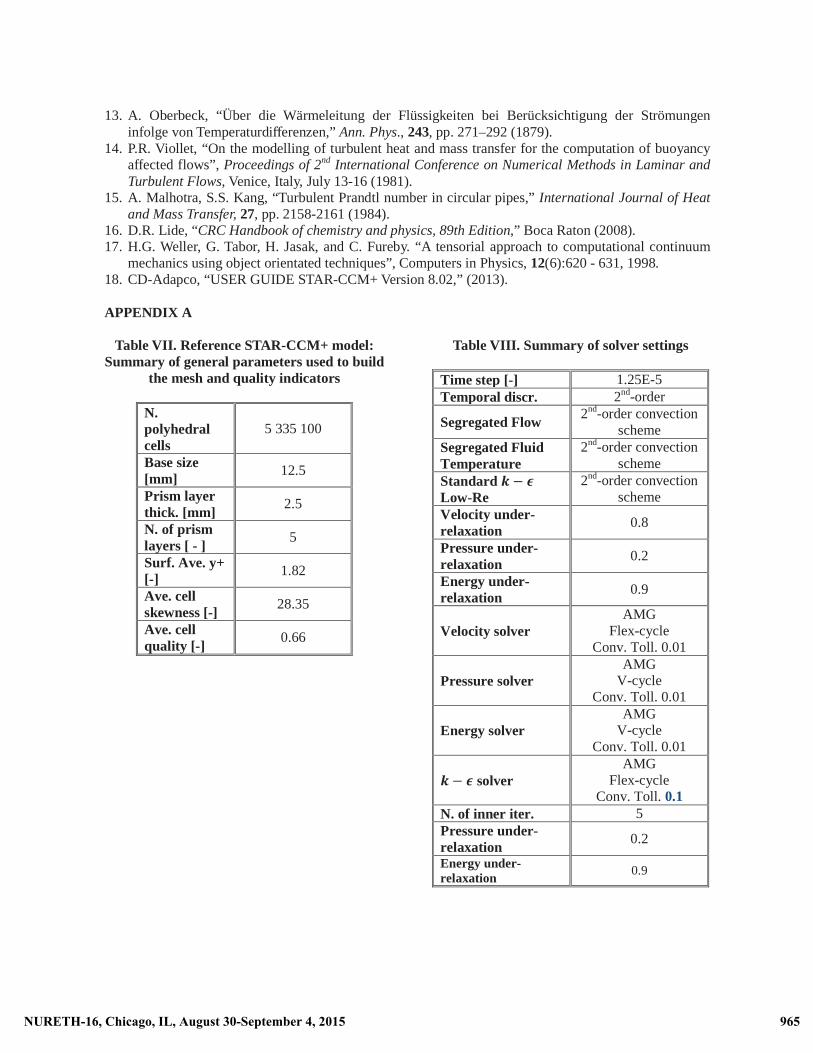
Table VII. Reference STAR-CCM+ model: Summary of general parameters used to build

the mesh and quality indicators

N. polyhedral cells

5 335 100

Base size [mm] 12.5

Prism layer thick. [mm] 2.5

N. of prism layers [ - ] 5

Surf. Ave. y+ [-] 1.82

Ave. cell skewness [-] 28.35

Ave. cell quality [-] 0.66

Table VIII. Summary of solver settings

Time step [-] 1.25E-5Temporal discr. 2nd-order

Segregated Flow 2nd-order convection scheme

Segregated Fluid Temperature

2nd-order convection scheme

Standard , � -Low-Re

2nd-order convection scheme

Velocity under-relaxation 0.8

Pressure under- relaxation 0.2

Energy under- relaxation 0.9

Velocity solver AMG

Flex-cycle Conv. Toll. 0.01

Pressure solver AMG

V-cycle Conv. Toll. 0.01

Energy solver AMG

V-cycle Conv. Toll. 0.01

, � - solver AMG

Flex-cycle Conv. Toll. 0.1

N. of inner iter. 5Pressure under- relaxation 0.2

Energy under- relaxation 0.9


Documents

Assessment of OpenFOAM CFD Toolbox for Gravity driven …glc.ans.org/nureth-16/data/papers/13200.pdf · 2015-08-12 · ASSESSMENT OF OPENFOAM CFD TOOLBOX FOR GRAVITY DRIVEN MIXING