1

Assessment of leaf cover and crop soil cover in weed harrowing research using

digital images J RASMUSSEN*, M NØRREMARK2) & BM BIBBY3) *Department of Agricultural Sciences, Faculty of Life Sciences, University of Copenhagen, Taastrup, Denmark, _Department of Agricultural, 2)Engineering, Faculty of Agricultural Sciences, University of Aarhus, Denmark, and 3)Department of Biostatistics, University of Aarhus, Aarhus, Denmark

SHORT TITLE: Assessment of crop soil cover

SUMMARY

Objective assessment of crop soil cover, defined as the percentage of leaf cover that has been buried

in soil due to weed harrowing, is crucial to further progress in post-emergence weed harrowing

research. Up to now, crop soil cover has been assessed by visual scores, which are biased and

context dependent. The aim of this study was to investigate whether digital image analysis is a

feasible method to estimate crop soil cover in the early growth stages of cereals. Two main

questions were examined: (1) how to capture suitable digital images under field conditions with a

standard high-resolution digital camera and (2) how to analyse the images with an automated digital

image analysis procedure. The importance of light conditions, camera angle, size of recorded area,

growth stage and direction of harrowing were investigated in order to establish a standard for image

capture and an automated image analysis procedure based on the excess green colour index was

developed. The study shows that the automated digital image analysis procedure provided reliable

estimations of leaf cover, defined as the as the proportion of pixels in digital images determined to

be green, which were used to estimate crop soil cover. A standard for image capture is suggested

and it is recommended to use digital image analysis to estimated crop soil cover in future research.

The prospects of using digital image analysis in future weed harrowing research are discussed.

2

Keywords: Physical weed control, crop damage, crop tolerance, crop resistance, crop recovery,

digital image analysis, the excess green colour index

Correspondence: J Rasmussen, Department of Agricultural Sciences, The Royal Veterinary and

Agricultural University, Højbakkegaard Allé 9, DK-2630 Taastrup, Denmark. Tel: (+45) 35 28 34

56; Fax (+45) 35 28 33 84; E-mail: jer[a]life.ku.dk

.

3

Introduction

In a recent paper on guidelines for physical weed control research, Vanhala et al. (2004) emphasise

the need of unbiased methods to assess the immediate crop damages associated with harrowing.

The importance of crop damage associated with weed harrowing has often been demonstrated

(Jensen et al., 2004) and Rasmussen (1991; 1993a) showed that crop soil cover is a valuable input

in predictive models that aim to determine the optimal intensity of harrowing.

The immediate crop response to harrowing is most often expressed in terms of crop soil cover,

which is the percentage of the above ground crop parts that have been buried in soil (Rasmussen,

1991). This measure is assessed by visual scores, which are context dependent and biased. Even

trained people assess crop soil cover rather individually. One assessor may estimate a specified

treatment at 20% crop soil cover while another may estimate it at 40% (Rasmussen et al., 1997).

Nevertheless, crop soil cover has been and still is used for the lack of any better (Jensen et al.,

2004). The biased nature of visual scores is not vital in experiments where the main objective is to

compare different treatments with the same experiment. However, when results from different

experiments are of interest, it is indeed very problematic to use visual ratings. For example, Jensen

et al. (2004) quantified the ability of lupin (Lupinus albus L. and L. luteus L.) to resist and tolerate

crop soil cover from post-emergence weed harrowing without being able to make reliable

comparisons to previous studies in pea (Pisum sativum L.). They doubted that their assessments of

crop soil cover in lupin were comparable to those in earlier studies in pea conducted by Rasmussen

(1993b). In consequence, visual assessment of crop soil cover hampers communication and learning

within the scientific community.

4

Crop soil cover is mainly used in Europe (Kurstjens & Kropff, 2001, Jensen et al., 2004, Melander

et al., 2005) whereas most research papers from USA and Canada express crop damage as crop

density reductions (Mohler & Frisch, 1997; Leblanc & Cloutier, 2000). Jensen et al. (2004)

discussed advantages and disadvantages of both measures and concluded that crop soil cover is the

only practicable real-time method in cereals and grain legumes, because it is impossible to

distinguish and count single crop plants immediately after harrowing. Plants are more or less buried

in soil, which make them inseparable.

Previously, two objective assessment methods of crop soil cover have been tried out: (1) wooden

sticks placed in crop rows to measure the height of the ridges created by the mechanical implements

(Melander, 1997; Cirujeda et al., 2003; Melander et al., 2003) and (2) photoelectric sensor

techniques where light reflectance from the crop canopy is measured by sensors (Rasmussen, 1996;

Rasmussen et al., 1997; Engelke, 2001; Hansen, 2005).

Wooden sticks are not useful for post-emergence weed harrowing because harrowing has no ridging

effect but the method has some potential in row-cultivation where soil is thrown into the rows.

There has been an increase in work on remote sensing by photoelectric sensors within site-specific

weed management (Gerhards & Christensen, 2003; Scotford & Miller, 2005) but results in the

context of weed harrowing are either negative or inconclusive when trying to establish a standard

method (Rasmussen, 1996; Rasmussen et al., 1997; Engelke, 2001, Hansen, 2005).

Rasmussen (1996) and Rasmussen et al. (1997) showed positive correlations between crop soil

cover assessed visually and by photoelectric sensors but the relation between assessments was

5

context dependent. Rasmussen et al. (1997) concluded that variability in ground colour rendered

sensor assessments inaccurate. Engelke (2001) found that the precision of photoelectric sensors

used in the early growth stages of cereals was too low to be useful in automated adjustments of

weed harrowing. Hansen (2005) used photoelectric sensors to investigate whether different barley

genotypes responded differently to weed harrowing but without indicating the reliability of his

assessments.

In a recent review on canopy spectral remote sensing, Thorp and Tian (2004) concluded that the

presence of variable soil backgrounds still complicates the spectral response and hinders the

analysis of vegetative cover. Unfortunately, the review was mostly concerned with the canopy

reflectance in the near infrared (NIR) and red wavebands. The study by Marchant et al. (2001) who

utilized three wavebands, red, near-infra-red (NIR) and green, was not included in the review. They

obtained satisfactory segmentation of vegetation from background with a combination of these three

wavebands plus introduction of a novel classification method (alpha-method). Unfortunately, this

method requires a dedicated sensor and it has not been tested in crops that have been disturbed by

mechanical weed control.

In order to develop a standard for objective and reproducible assessment of crop soil cover, we

chose digital image analysis instead of photoelectric sensors because digital cameras are widespread

and because image processing is used widely in research on leaf cover assessment (Thorp and Tian,

2004).

6

Our objectives were (1) to investigate whether digital image analysis provides reliable estimations

of crop soil cover in the early crop growth stages of cereals and (2) to suggest a standard for the

image capture procedure.

Materials and methods

Terminology and experimental approach

In this study, leaf cover is defined as the proportion of pixels in digital images determined to be

green, and crop soil cover, defined as the percentage of leaf cover that has been buried in soil due to

weed harrowing, is calculated as the leaf cover differences between control plots and harrowed

plots divided by the leaf cover in control plots within each block replication. Leaf cover and crop

soil cover are both expressed in percentage by multiplying by 100.

This study focus on factors that could be assumed to influence the estimation of leaf cover and

thereby crop soil cover from digital images such as camera tilt angle, light conditions, size of

recorded areas, direction of harrowing and growth stage of the crop. It is based on an innovative

approach, which started with two main questions, (1) how to acquire useful digital images with a

standard high-resolution digital camera (the image capture challenge) and (2) how to develop an

appropriate algorithm and automated analysis procedure within a standard software package (the

image analysis challenge) to calculate the proportion of green pixels in digital images. There was no

attempt to discriminate crop and weeds because it was considered unimportant in the perspective of

early post-emergence weed harrowing. In most cases weeds are assumed to make up only a few

percent of the total leaf cover.

7

The challenges associated with the image capture and the digital image analysis were mutually

connected. The image-processing procedure was changed several times during the study to cope

with the different characteristics of the images acquired and the work with the image analysis also

influenced the image-capture scheme.

The innovative working process with the image analysis challenge is described and illustrated in the

materials and methods section, whereas the outcome of the work with the image capture challenge

is described the result section.

Field experiments

Digital images originated from two field experiments (experiment 1 and 2) with weed harrowing in

organic winter wheat (cv Complet) mixed with approximately 10% winter rye (cv Caroass). The

mixture was arranged in order to guarantee that the harvested crop, could be distinguished from

other non-organic winter wheat.

Both experiments were conducted on a sandy loam at Bakkegården, which is an experimental farm

owned by The Royal Veterinary and Agricultural University, Denmark. The farm is organic, which

means that pesticides were not used.

Experiment 1 was originally planned to investigate the importance of timing of weed harrowing in

order to achieve efficient weed control and positive crop yield response, and the results have been

reported elsewhere (Rasmussen & Nørremark, 2006).

8

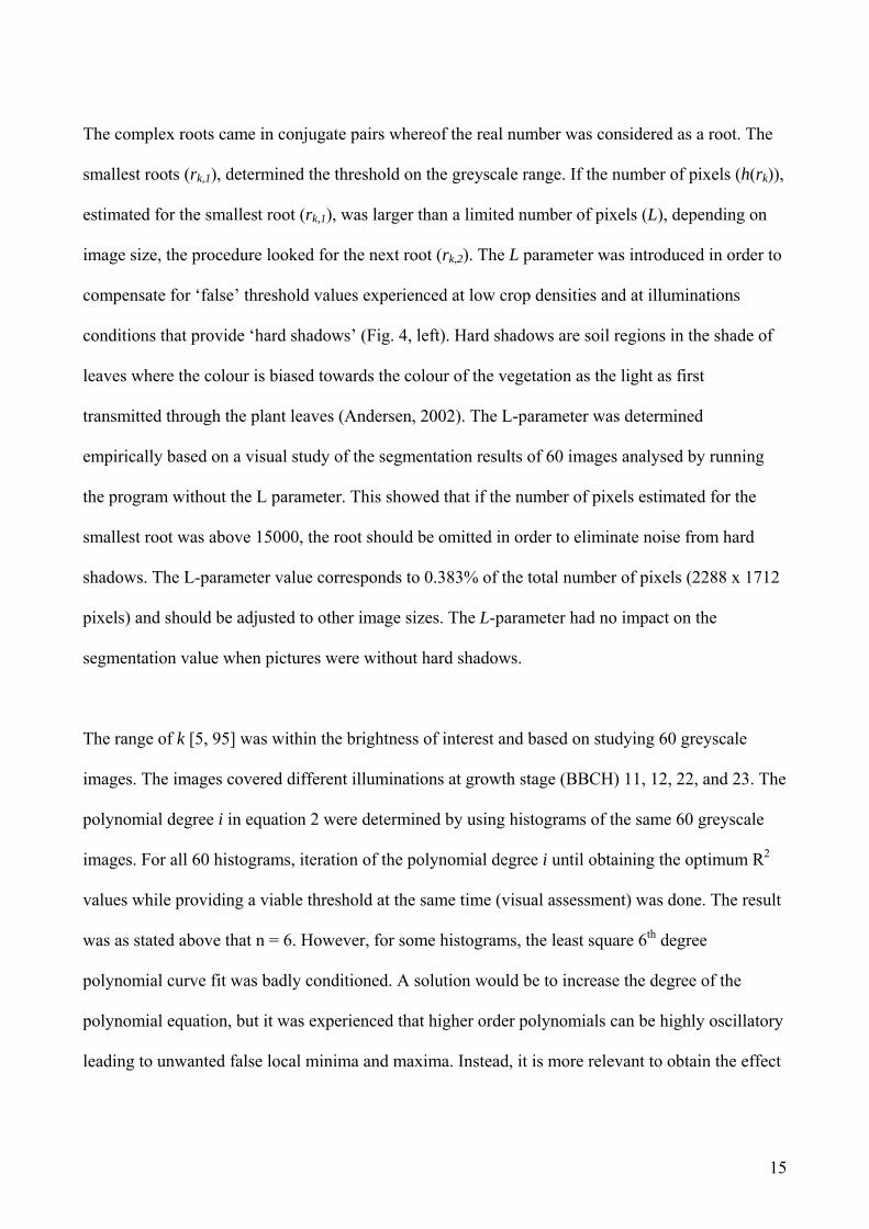
Weed harrowing was carried out at three growth stages (BBCH), 12, 22 and 23 and in a

combination of all growth stages (12+22+23), hereafter called the combined growth stage.

Harrowing was on 9 December 2003, 14 April 2004 and 30 April 2004. At each growth stage, the

crop was harrowed in the same direction 1, 2, or 3 times on the same day to create a progressive

series of intensities. The planned targets of the graded levels of harrowing in each of the three

specific growth stages were 0 (control), 30, 60 and 90% crop soil cover in order to cover the whole

range of intensities from normal to very aggressive. The practical adjustment of the aggressiveness

of harrowing was adjusted on the basis of visual assessments of the whole plots. Driving speed and

tine angle was adjusted so one pass gave approximately 30% crop soil cover. After the settings of

driving speed and tine angles had been chosen, all plots were harrowed with the same adjustment.

Harrowing was done with a 3 m wide weed harrow manufactured by Einböck (Einböck GmbH &

CoKG, A-4751 Dorf an der Pram, Austria). At growth stage 12, the angle of tines was adjusted to

the highest negative value possible (Vanhala et al., 2004) giving a very gentle treatment. Driving

speed was 3 km h-1. At growth stage 22 and 23, the angle of tines was adjusted to the highest

positive value possible (Vanhala et al., 2004) giving the most aggressive treatment. Driving speed

was 8 km h-1. Higher driving speed did not increase the intensity in terms of crop soil cover.

The planned targets were practicable in autumn 2003 but not in spring 2004 where the soil was too

compacted to achieve high degrees of crop soil cover. Based on visual assessments, about 20% crop

soil cover was achievable after 3 successive passes at growth stage 22 (14 April 2004) and at

growth stage 23 (30 April 2004) only about 20% crop soil cover was achievable.

9

Growth stage was assigned to main plots, with the four intensities of harrowing applied as a sub-

plot treatment. Growth stage was on main plots because this saved time when plots were harrowed.

Each sub-plot was 14 m long and 3 m wide.

All digital images were taken in 2004, which means that there were no recordings from the earliest

growth stages in autumn 2003. To investigate the utility and possible limitations of the digital

image analysis procedure in very early growth stages, a second experiment (experiment 2) was

carried out in autumn 2004 to question whether it is possible to discriminate treatments when leaf

cover approaches 1-3% of the ground surface.

In experiment 2, three progressive series of harrowing with 4 graded levels of harrowing was

carried out in growth stage (BBCH) 11 when the first developed leaf was about 4-5 cm long. One

series was harrowed along the crop rows, one across the crop rows and one in both directions,

which means that harrowing was done in plots that were drilled in two perpendicular directions

(double seed rate). The double seed rate was used because it was doubted whether it would be

possible to discriminate treatments at the normal seed rate due to very low levels of leaf cover. The

experiment was designed as three randomised block experiments within each direction; along,

across and both. The angle of the tine on the Einböck harrow was adjusted to give the gentlest

treatment possible, and driving speed was adjusted to give the graded levels of treatment (0 km h-1,

2 km h-1, 3.5 km h-1 and 5 km h-1). The driving speed was adjusted instead of the number of passes

as in experiment 1 because an increasing number of passes created too aggressive treatments.

Image capture

10

In all photo sessions, four images were taken in each plot, and a total of 2112 images were recorded

and analysed. Of these, 512 images were used to interpret the weed control experiment (Experiment

1) as presented in Rasmussen & Nørremark (2006).

The images, 2288 pixels horizontally by 1712 pixels vertically with 24-bit depth, were taken using a

red, green, blue (RGB) digital camera, Olympus C750UZ (Olympus Optical Co., Ltd.). An 11 mm

focal length lens was used with a fixed F-stop of 3.2. The digital image analysis procedure makes

no special demands on the camera in terms of filters, white balancing, shutter speed or aperture

value. The only requirement is that the images are focused and correctly exposed. To avoid random

variation in the camera angle, a tripod was used to fix the position of the camera.

To investigate the importance of light source, a series of images were captured in bright and diffuse

sunlight on 14 April and 30 April in experiment 1 (Table 1). To create diffuse sunlight, the sun was

screened with a bright cloth, which made shadows from the crop plants imperceptible. Images

captured on 14 April were taken with camera tilt angle 300 and on 30 April with camera angle 450

according to Fig. 1.

Fig. 1 Illustration of camera angles relative to the ground plane and the direction of harrowing

11

To investigate the importance of the directed angle of the camera relative to the ground plane, three

different angles were compared, 00, 300 and 450 (Table 1). By increasing angles, the camera was

turned in the same direction as the plots were harrowed for the majority of recordings (Fig. 1).

However, also one camera angle against driving direction was tried out on 30 April at growth stage

23 in bright and diffuse sunlight (Table 1).

12

Table 1 Image capture schemes from experiment 1.

Harrowing dates

Angle of camera

according to Fig. 1

Growth stage 12

9 Dec. 2003

Growth stage 22

14 Apr. 2004

Growth stage 12, 22,

and 23

9 Dec. + 14 Apr. + 30

Apr.

Image capture dates and conditions

Along driving direction Overcast Sunlight

screened

Direct

sunlight

Sunlight

screened

Direct

sunlight

0o 7 Apr. 04‡ 14 Apr.

04‡

30 Apr.

04‡

30o 7 Apr. 04‡ 14 Apr.

04†,‡

14 Apr.

04†

45o 7 Apr. 04‡ 14 Apr.

04‡

30 Apr.

04†,‡,§

30 Apr.

04†,§

Against driving direction

45o 30 Apr.

04§

30 Apr.

04§ †Data is presented in Fig. 5 ‡Data is presented in Fig. 6 §Data is presented in Fig. 7

As the camera height over ground was kept constant at 110 cm, images represented increasing areas

(in the range of 0.32 m2 to 1.00 m2) and decreasing resolutions (mm2/pixel) by increasing camera

angles. To investigate the importance of area and to break the correlation between area and camera

angle, two series of images covering 0.23 m2 and 0.32 m2, respectively, were acquired with camera

angle 00 on 7 April in plots that were harrowed on 9 December 2003 in experiment 1. Camera

height was reduced in order to reduce area.

13

To investigate whether the digital image analysis could discriminate treatments carried out at very

early growth stages, a series of images were captured on 2 November 2004 in experiment 2 in a

crop with only one 4-5 cm leaf (BBCH 11). The camera angle was 0o and images were captured in

bright sunlight. All plots were photographed before and after treatment on the same day to

investigate whether pre-treatment images would improve the accuracy of the estimated crop

response curves.

The image analysis procedure

The objective of the image analysis was to obtain a binary image where green plant leaves were

segmented from soil surface, shadows, stones, dead plant residues and other debris. In a standard

colour camera the spectrum received has a dimension of three, corresponding to a response in the

red (R) (560-700nm), green (G) (480-600nm), and blue (B) (380-480nm) bands giving the so-called

RGB tristimulus. Usually 24 bits of information for each pixel is stored in the image from standard

digital cameras. This is apportioned with 8 bits each for red, green and blue, giving a range of 256

possible intensities for each hue. An image can be defined as a two-dimensional function f(x, y),

where x and y are spatial (plane) coordinates, and the amplitude of f at any pair of coordinates (x, y)

is called the intensity of the image at that point.

The segmentation was based on the three-component (RGB) data vector that describes each point in

the image. The first stage of the segmentation, transforms the original RGB image into greyscale

(monochrome) image by applying the excess green index introduced by Woebbecke et al. (1995)

and Meyer et al. (1998):

y,xy,xy,xy,x BRG2Q −−×= (Equation 1)

14

where Rx,y, Gx,y, Bx,y and Qx,y are the non-normalized red, green, and blue intensities (0-255) and

excessive green index respectively for each pixel coordinate (x, y) in the image. Q was rescaled into

the range of 0-255 by adding number of pixels for greyscale values below this range to 0 and above

this range to 255.

In the resulting greyscale image, green plants appear bright in contrast to a dark, almost uniform

background where the soil surface, including shadows, stones, straw, and other debris have

disappeared.

The next step was to determine the greyscale threshold (Fig. 2), which sets the contrast breakpoint

between pixels containing vegetation and pixels containing non-vegetation. The threshold is

depending on illumination conditions. That is, the brightness magnitude varies if the greyscale

image of vegetation and non-vegetation is light, dark, low-contrast or high-contrast (Fig. 3).

Therefore, the threshold should be set automatically in order to adjust for differences in

illumination.

The automatic threshold determination consists first of a least square polynomial curve fit to a

histogram of the greyscale image (Equation 2 and Fig. 2). The histogram has greyscale levels in the

range [0, 28-1] and is a discrete function h(rk) = nk, where rk is the kth greyscale value and nk is the

number of pixels in the image having greyscale value rk.

( ) ∑=

=n

i

ikik rarh

0

(Equation 2)

where k = 5,...., m, and m = 95 (i.e. a section of the greyscale value range), i = 0,...., n and n = 6 and

ai is the coefficients of the polynomial. Then, the local minima and maxima for h(rk) were found by

determining both real and complex roots of the derivative of the 6th degree polynomial (h′(rk) = 0).

15

The complex roots came in conjugate pairs whereof the real number was considered as a root. The

smallest roots (rk,1), determined the threshold on the greyscale range. If the number of pixels (h(rk)),

estimated for the smallest root (rk,1), was larger than a limited number of pixels (L), depending on

image size, the procedure looked for the next root (rk,2). The L parameter was introduced in order to

compensate for ‘false’ threshold values experienced at low crop densities and at illuminations

conditions that provide ‘hard shadows’ (Fig. 4, left). Hard shadows are soil regions in the shade of

leaves where the colour is biased towards the colour of the vegetation as the light as first

transmitted through the plant leaves (Andersen, 2002). The L-parameter was determined

empirically based on a visual study of the segmentation results of 60 images analysed by running

the program without the L parameter. This showed that if the number of pixels estimated for the

smallest root was above 15000, the root should be omitted in order to eliminate noise from hard

shadows. The L-parameter value corresponds to 0.383% of the total number of pixels (2288 x 1712

pixels) and should be adjusted to other image sizes. The L-parameter had no impact on the

segmentation value when pictures were without hard shadows.

The range of k [5, 95] was within the brightness of interest and based on studying 60 greyscale

images. The images covered different illuminations at growth stage (BBCH) 11, 12, 22, and 23. The

polynomial degree i in equation 2 were determined by using histograms of the same 60 greyscale

images. For all 60 histograms, iteration of the polynomial degree i until obtaining the optimum R2

values while providing a viable threshold at the same time (visual assessment) was done. The result

was as stated above that n = 6. However, for some histograms, the least square 6th degree

polynomial curve fit was badly conditioned. A solution would be to increase the degree of the

polynomial equation, but it was experienced that higher order polynomials can be highly oscillatory

leading to unwanted false local minima and maxima. Instead, it is more relevant to obtain the effect

16

of averaging out questionable data points, rather than distorting the curve to fit data exactly.

Nevertheless, the methodology was always able to find a root that could set a viable greyscale

threshold.

The obtained greyscale threshold was then used to transform the rescaled excess green image into a

binary image. The transformation assigned 0 to all of the pixels below the threshold value and 1 to

all of the pixels above the threshold (i.e. vegetation). Finally, a 3 by 3 median filter was applied to

reduce the binary image noise due to segmentation errors. Thus, it was assumed that a group of four

or less connected pixels was noise. From the filtered image, the proportion of white pixels

corresponding to green pixels on the original colour image was counted and termed leaf cover.

By applying the procedure as outlined above, each image resulted in one value, leaf cover, which

was the proportion of pixels that were determined to be green in the original image. The leaf cover

was expressed in percentage and could easily be related to crop soil cover as the percentage of loss

of leaf cover as a result of harrowing. The image processing approach did not discriminate crop and

weeds. An experienced drawback of the segmentation process is that plant leaves or leaf parts will

not be recognised as vegetation when illumination and plant conditions provides 100% surface

reflection of incident light.

The analysis procedure was programmed in MATLAB and MATLAB Image Processing Toolbox

(MathWorks, Inc, MA, USA). For 20 images the clock time at the beginning and ending of

processing was stored so that the elapsed time to analyse each image could be calculated. MATLAB

ran on a standard laptop PC with a Pentium M processor operating at 1.6 GHz under a Windows XP

17

operating system. The mean elapsed time of the segmentation was 1.77 s with a standard deviation

of 0.03s.

R2 = 0.7512

0

5000

10000

15000

20000

25000

30000

0 5 10 15 20 25 30 35 40 45 50 55 60 65 70 75 80 85 90 95 100Greyscale

Num

ber o

f pix

els

L

-200.0

-150.0

-100.0

-50.0

0.0

50.0

100.0

150.0

200.0

0 5 10 15 20 25 30 35 40 45 50 55 60 65 70 75 80 85 90 95 100

Greyscale

Der

ivat

ive

of h

isto

gram

pol

ynom

ial

Fig. 2 Example of polynomial fit to histogram (left) and the derivative of the histogram polynomial

(right). The found threshold values on the greyscale were 26.4 (the real part of a complex root),

60.3, 69.0, and 87.7. The data is from the segmentation presented in Fig. 3, left column. For the

illustrated segmentation the threshold value 26.4 was used.

18

Fig. 3 Examples of images taken under shielded (left) and un-shielded conditions (right) on a sunny

day and the corresponding binary images from the digital image analyses. Leaf cover was 15.9% for

both images calculated on basis of the automated image processing segmentation. Threshold values

of 25.4 (left) and 29.9 (right) was determined by the segmentation process. Images are from control

plots that have not been harrowed.

19

Fig. 4 Examples of images with low and high leaf cover in harrowed plots and the corresponding

binary images. The left column image was taken under illumination conditions that resulted in ‘hard

shadows’ and the right column image in “soft shadows”. The low leaf cover was determined 2.57%

and the high leaf cover was determined to 53.4%. Images are from plots that have been harrowed.

Statistics

To investigate whether digital image analysis provides reliable assessments of the immediate crop

response, percentage leaf cover was used in the statistical analysis and not crop soil cover. Leaf

cover is a more appropriate response parameter than crop soil cover, because it is an absolute

measure in opposite to crop soil cover, which is expressed relative to untreated plots.

Regression analysis was used to describe how light conditions, camera angle, growth stage, size of

photographed area and angle of camera and direction of harrowing influenced the digital assessment

of leaf cover. Number of passes (intensity of harrowing) was the independent regression variable

(covariate) and leaf cover was the response variable in different mixed models with light condition,

camera angle, direction of harrowing, growth stage, size of photographed area and block as

qualitative variables. Regression models were tested against analysis of variance models to test the

20

lack-of-fit. In order to omit non-significant factor or factor combination effects on parameters,

successive approximative F-tests were made to reduce the complexity in models. Statistical

analyses of leaf cover were performed with PROC MIXED in SAS (SAS version 8, SAS Institute,

Cary, USA). In all cases, it was decided to analyse the logarithm of the leaf cover after inspecting

the residuals.

Light conditions were analysed starting with a mixed linear model with harrowing, light conditions

and time (and all interactions) as fixed effects, and plot, block and the interaction between time and

block (whole plot) as random effects. Due to the fact that the variation within plots decreased with

angle, the within plot standard deviation was allowed to depend on angle. Estimated regression lines

based on the reduced model are presented in Fig. 5.

Camera angle and size of photographed area were analysed starting with a mixed linear model with

harrowing, angle, and time (and all interactions) as fixed effects, and plot, block and the interaction

between time and block (whole plot) as random effects. As variation within plots increased with

angle, the within plot standard deviation was allowed to depend on angle. Estimated regression lines

based on the reduced model are presented in Fig. 6. The importance of size of the photographed

area was analysed by using the same mixed linear model, only replacing angle with size (within plot

variation decreased with size).

Direction of camera was analysed starting with a mixed linear model with harrowing, light, and

camera direction as fixed effects (with all interactions). Block, plot, and the interaction between plot

and direction (sub-plot) were included as random effects. There was a larger within plot variation

against the driving direction compared to along the driving direction, and the within plot standard

21

deviation was allowed to depend on driving direction. Estimated regression lines based on the

reduced model are presented in Fig. 7.

The importance of harrowing direction in experiment 2 was analysed using the same model, only

replacing camera direction with harrowing direction. Estimated regression lines based on the

reduced model are presented in Fig. 8.

Results

Light conditions

Analysis of variance showed that there was no significant three-way interaction between growth

stage, harrowing, and light conditions (P = 0.08) and subsequently no interaction between

harrowing and light conditions (P = 0.61) when leaf cover was the response parameter. The

remaining two interactions were significant, between harrowing and time (P = 0.04) and between

time and light (P = 0.005). Regression analysis showed that number of harrowings could be

included in the statistical analysis as a covariate and that leaf cover decreased exponentially by

increasing number of passes with the harrow. No significant light effect was found on 14 April (P =

0.61) but on 30 April the general level of percentage leaf cover was assessed as 10% (95%-CI: 7% -

13%) higher in diffuse sunlight compared to direct light (Fig. 5). The assessed impact of harrowing

was unaffected by light conditions in terms of percentage reduction of leaf cover but growth stage

influenced the impact of harrowing. On 14 April each pass reduced leaf cover by 11% (95%-CI: 6%

- 16%) and on 30 April by 19% (95%-CI: 15% - 22%) independently of light source.

22

Fig 5 Impact of light source on the assessment of leaf cover on 14 April and 30 April. ■= direct and

▲= diffuse sunlight. Observed treatment means and estimated regression lines. Further details in

Table 1.

Camera tilt angle

Analysis of variance showed that there was a clear interaction between camera tilt angle and growth

stage (P < 0.0001), number of harrowings and growth stage (P = 0.022), but no three way

interaction (P = 0.90) or interaction between harrowing and camera angle (P = 0.22) when leaf

cover was the response parameter. Regression analysis showed that number of harrowings could be

included in the analysis as a covariate showing that leaf cover decreased exponentially by

increasing number of passes with the harrow.

Camera angles 00 and 300 gave inseparable assessments on 7 April and 14 April (P = 0.60) but the

within plot standard deviation was clearly decreased by increasing camera angle (P < 0.0001).

23

The assessed impact of harrowing was unaffected by camera angle in terms of percentage reduction

of leaf cover, whereas growth stage influenced the impact (Fig. 6). On 7 April, each pass reduced

leaf cover by 8% (95%-CI: 3% - 12%), on 14 April by 14% (95%-CI: 10% - 19%), and on 30 April

by 20% (95%-CI: 16% - 24%) independently of camera angle.

Fig. 6 Influence of camera tilt angle on the assessment of leaf cover on 7 April, 14 April, and 30

April. ▲ = average of 00 and 300 (except on 30 April where data on 300 did not exist) and ■= 450.

Further details in Table 1. Observed treatment means and estimated regression lines.

When the camera was angled away from 00, it was important whether the direction was along or

against the driving direction (+/- 450). There was no three-way interaction between camera

direction, harrowing, and light (P = 0.65). Subsequently there was no interaction between

harrowing and light (P = 0.67) or between camera direction and light (P = 0.54). As in the previous

analyses, harrowing could be included as a covariate. There was no effect of direction on the

intercept (P = 0.73) but light conditions influenced the intercept (P < 0.0001) (Fig. 7). An average

leaf cover was assessed as being 9% (95%-CI: 5% - 13%) higher in plots with shaded light

24

compared to bright sunlight. The assessed impact of harrowing was unaffected by light conditions.

The impact, however, was influenced by camera direction. When camera direction was along the

driving direction (+450), each pass was estimated to reduce leaf cover by 19% (95%-CI: 15% -

23%) and when the direction was against the driving direction (-450) by 25% (95%-CI: 21% - 28%).

Changing leaf angles by increasing number of passes caused the interaction between the camera

direction and harrowing. After 3 passes the crop plants were clearly angled in the driving direction.

Fig. 7 Influence of camera direction relative to driving direction on the assessment of leaf cover on

30 April. ▲ = camera direction along driving direction and ■ = camera direction against driving

direction. Broken lines indicate shaded sunlight and full lines bright sunlight. Observed treatment

means and estimated regression lines. Further details in Table 1.

Size of recorded area

There was a clearly larger variation in the determined leaf cover when small areas (0.23 m2) were

photographed compared to large areas (0.32 m2) (P = 0.0005). There was no systematic effect of

size on leaf cover (all P values associated with size and interactions including size were larger than

25

0.24). The within plot variance in large area images was only 53% of the within plot variance in

small area images.

Direction of harrowing in early growth stages

Covariance analysis including pre-treatment assessment of leaf cover as a covariate did not improve

the statistical analysis of leaf cove after treatments due to non-significant effects of the pre-

treatment assessment. In consequence, pre-treatment assessment was excluded from further

analysis.

There was no interaction between direction of harrowing and forward speed (P = 0.76) and the

analysis showed that each km h-1 increase in driving speed reduced leaf cover by 13% (95%-CI: 9%

- 16%) independently of direction of harrowing (Fig. 8). There was no indication that the crop

response was better assessed in plots that were drilled both ways and thereby had a higher leaf

cover.

26

Fig. 8 Influence of harrowing direction in experiment 2 relative to forward driving speed on the

assessment of leaf cover on 2 Nov. Observed treatment means and estimated regression lines.

Discussion

The main challenge in our study, in terms of the digital image analysis procedure, was to achieve

segmentation robustness in outdoor field images under varying lighting conditions and to automate

the digital image analysis. The image analysis procedure used was based on the discrimination of

plant and background by thresholding the excess green colour index (Mayer et al., 1998). Our

contribution to the generation of a standard procedure was that we automated the determination of

the grey level threshold, which sets the breakpoint between vegetation and non-vegetation. A fixed

threshold as used in other studies (Meyer et al., 1998; Tang et al., 1999) did not apply in our study

with different growth stages and light conditions.

We evaluated that the automated procedure provided reliable assessments. However, we did not

apply a “true” reference, which could quantify the accuracy of the automated image analysis

procedure. Some authors (Ngouajio et al., 1998) compared operator-assisted classification of pixels

(crop, weeds and soil) with automated digital image analysis, but this method was too labour

intensive in our study. We controlled our image analysis procedure by careful comparison of the

original colour images and the segmented binary images by randomly checking a number of images

representing different lighting conditions and growth stages in the range of 1% to 40% leaf cover.

Compared with the visual assessments of crop soil cover, which may by be influenced by a factor 2

of the individual assessor (Rasmussen et al., 1997), our digital image analyse procedures represents

a huge improvement in precision.

27

We did not compare our digital image algorithm with modified forms of the excess green colour

index (Ribeiro et al, 2005) or our ordinary digital camera with more sophisticated 3CCD cameras

(Onyango & Marchant, 2001). We were satisfied with the excess green colour index because our

algorithm was fully automatic i.e. no manual settings of parameters were needed and it worked for

image capture with auto white balancing. This was not the case for other methods used for

vegetation segmentation in digital images (Onyango & Marchant, 2001; Grundy et al., 2005;

Ribeiro et al., 2005).

Our image analysis procedure is fairly simple compared to image analysis systems that discriminate

crop and weeds (Lemieux et al., 2003; Onyango & Marchant, 2003, Grundy et al., 2005) and our

next step will be an attempt to convert the procedure into a simple software package that can be

used by non-specialists into image analysis or without sophisticated software.

In weed science, leaf cover used in competition models is assessed as the vertical projection of plant

canopy on the ground (Ngouajio et al., 1998; Lemieux et al., 2003), which is closely related to leaf

area in early growth stages. We used different camera tilt angles because we focused on plant

populations with different degrees of disturbance. It could be hypothesised that vertical projection

would result in overestimation of leaf cover in harrowed plots because harrowing affects the

deflection of the crop plants and may even flatten them in the driving direction. In contrast, it could

be hypothesised that angled projections in the driving direction, would result in overestimation of

leaf cover in undisturbed plots. Interactions between camera angle and number of passes with the

harrow were expected if camera angle is important for the assessment of leaf cover. Our study,

however, showed no significant interactions between camera angle and the effects of weed

harrowing in terms of percentage reduction of leaf cover (Fig. 6), which indicates that vertical

28

projection is suitable to assess leaf cover in crops that have been disturbed by harrowing. Camera

angles against the driving direction, however, clearly influenced the assessed impact of harrowing

(Fig. 7) and should be avoided.

Based on the findings, vertical projections should generally be preferred and definitely be used if

driving direction is variable within a field or experiment. An angled camera may result in

overestimation of the general level of leaf cover but the estimated impact of weed harrowing in

terms of percentage reduction of leaf cover (crop soil cover) was not affected (Fig 6).

The captured area in the image recording procedure is inversely related to image resolution. The

resolutions used in this study were in the range of 0.06-0.25 mm2/pixel, which is a higher resolution

than 1 mm2/pixel used by Ngouajio et al. (1998). Ngouajio et al. (1998) reported how increasing

recording area (0.33 to 1.63 m2) influenced leaf cover assessments at the expense of resolution (0.6

to 3.2 mm2/pixel). They found that average leaf cover estimates from increasing areas were less

variable even if the resolution was lower. Their image analysis procedure, however, was not

automated and the resolution limit is in our automated programme is unknown. It is assumed that

the resolution used in this study could be further reduced.

Objective estimations of leaf and crop soil cover add new perspectives to research because post-

emergence weed harrowing is a trade-off between crop damage and weed removal effectiveness.

This explains why mechanical weed control may cause yield decrease compared with untreated

plots at low weed pressure and yield increase at high weed pressure as found by Rasmussen (2004)

and Rasmussen & Nørremark (2006).

29

Objective assessment of crop soil cover makes it practicable to distinguish two important aspects of

crop tolerance to weed harrowing, resistance and recovery. Resistance reflects the ability of the crop

to resist leaf cover reduction and recovery reflects the ability of the crop to regenerate from crop

soil cover in weed-free environments. In this perspective, crop tolerance is the combined capacity of

the crop to resist and recover from crop soil cover associated with harrowing. The importance of

gaining knowledge about crop tolerance was illustrated in the weed control experiment, which

constituted the basis of this methodology study. Crop resistance and crop recovery were highly

affected by timing of weed harrowing and of major importance in order to optimize weed harrowing

in terms of crop yield response (Rasmussen & Nørremark, 2006)

The lack of objective assessment of crop soil cover has resulted in oversimplified guidance and

decision support. In Denmark, it is recommended that crop soil cover should not exceed 10-20% in

spring cereals (Berthelsen, 2003). This guidance implies (1) that the specific range of crop soil

cover is generally reasonable and (2) that farmers are capable of forming fairly accurate estimates

of crop soil cover. Both preconditions are questionable. Weed species and densities, selectivity

conditions and crop tolerance all influence the range of acceptable crop soil cover. Experiments

have shown that increasing intensity of harrowing may result in yield gains in the entire range of 0-

80% crop soil cover under given conditions, whereas other conditions make it impossible to achieve

yield gains even at very low levels of crop soil cover (Rasmussen, 1991; 1993a).

Only few decision support models have considered post-emergence weed harrowing (Kristensen &

Rasmussen, 2002) and no systems have been developed to help farmers to adjust the intensity and

timing of harrowing. Kurstjens & Kropff (2001) developed a conceptual model of the harrowing

process, which helps to get an understanding of the involved mechanisms but their model is too

30

complicated to serve as the framework in a practical decision support system. A practical way to

integrate knowledge about crop tolerance in guidance and decision support systems still has to be

evolved.

Conclusion

This study shows that leaf cover and crop soil cover can be estimated from images captured by an

ordinary digital camera by using our automated digital image analysis procedure, which is based on

the excess green colour index. Our results show that images should be captures in stable lightning

conditions. The estimated values of crop soil cover were unaffected by lightning conditions under

the condition that they were constant. Shifting lightning conditions while images are captured add

experimental error to the estimated values and should be avoided. A camera angle of 00 (vertical

projection) is preferable because an angled camera influences the general level of assessment. As

for lightning conditions, the estimated values of crop soil cover were unaffected by camera angle

under the condition that the camera is angled along the driving direction of the harrows. Image

resolution of 0.25 mm2/pixel and four 0.32 m2 images per experimental plot in experiments with

four block replications provided high precision assessments. Larger recording areas at the expense

of image resolution would most likely improve assessment precision but this was not tested. In

conclusion, our study shows that digital image analysis provides a feasible method to assess crop

soil cover in weed harrowing research, and we recommend that the digital image analysis procedure

and the image capture standard proposed in this paper is used to quantify crop soil cover in future

research into post-emergence weed harrowing.

Acknowledgement

We would like to thank John R. Porter for his contribution to the improvement of the manuscript.

31

References

ANDERSEN HJ (2002) Outdoor computer vision and weed control. PhD dissertation, Computer

Vision and Media Technology Laboratory (CWMT), Aalborg University, June 2002. p. 154.

BERTELSEN I (2003) Økologisk ukrudtsbekæmpelse (Ecological weed control). Landbrugsforlaget,

Århus, Denmark.

CIRUJEDA A, MELANDER B, RASMUSSEN K & RASMUSSEN IA (2003) Relathionship between speed,

soil movement into the cenreal row and intra-row weed control efficacy by weed harrowing.

Weed Research 43, 285-296.

ENGELKE B (2001) Entwicklung eines Steuersystem in der ganzflächig mechanischen

Unkrautbekämpfung PhD Dissertation. Christian Albrechts Univerität, Kiel, Germany.

GERHARDS R & CHRISTENSEN S (2003) Real-time weed detection, decision making and patch

spraying in maize, sugarbeet, winter wheat and winter barley. Weed Research 43, 385-392.

GRUNDY AC , ONYANGO CM, PHELPS P, READER RJ, MARCHANT JA, BENJAMIN LR, MEAD A

(2005) Using a competition model to quantify the optimal trade-off between machine vision

capability and weed removal effectiveness. Weed Research, 45, 388-405

HANSEN PK (2005) Tolerance to weed harrowing in spring barley genotypes. In: Proceedings. The

13th European Weed Research Society (EWRS) Symposium, Bari, Italy. www.ewrs.org.

JENSEN RK, RASMUSSEN J & MELANDER B (2004) Selectivity of weed harrowing in lupin. Weed

Research 44, 245-253.

KRISTENSEN K & RASMUSSEN IA (2002) The use of a Bayesian network in the design of a decision

support system for growing malting barley without use of pesticides Computers and electronics

in agriculture 33, 197-217.

32

KURSTJENS DAG & KROPFF MJ (2001) The impact of uprooting and soil-covering on the

effectiveness of weed harrowing. Weed Research 41, 211-228.

LEBLANC ML & CLOUTIER DC (2001) Susceptibility of dry edible bean (Phaseolus vulgaris,

cranberry bean) to the rotary hoe. Weed Technology 15, 224-228.

LEMIEUX C, VALLEE L & VANASSE A (2003) Predicting yield loss in maize fields and developing

decision support for post-emergence herbicide applications. Weed research 43, 323-332.

MARCHANT JA, ANDERSEN HJ & ONYANGO CM (2001) Evaluation of an imaging sensor for

detecting vegetation using different waveband combinations. Computer and Electronics in

Agriculture 32, 101 – 107.

MELANDER B (1997) Optimization of the adjustment of a vertical axis rotary brush weeder for intra-

row weed control in row crops. Journal of Agricultural Engineering Research, 68, 39-50.

MELANDER B, CIRUJEDA A & JØRGENSEN MH (2003) Effects of inter-row hoeing and fertilizer

placement on weed growth and yield of winter wheat. Weed Research 43, 428-438.

MELANDER B, RASMUSSEN IA & BÀRBERI P (2005) Integrating physical and cultural methods of

weed control – examples from European research. Weed Science 53, 369-381.

MEYER GE, MEHTA T, KOCHER MF, MORTENSEN, DA & SAMAL A (1998) Textural imaging and

discriminant analysis for distinguishing weeds for spot sprayers. Transactions of the American

Society of Agricultural Engineers 41, 1189-1197.

MOHLER CL & FRISH JC (1997) Mechanical weed control in oats with a rotary hoe and tine weeder.

Proceedings Northeastern Weed Science Society, 51, 2-6.

NGOUAJIO M, LEMIEUX C, FORTIER JJ, CAREAU D & LEROUX GD (1998) Validation of an operator-

assisted module to measure weed and crop leaf cover by digital image analysis. Weed

Technology 12, 446-453.

33

ONYANGO CM & MARCHANT JA (2001) Physics based colour image segmentation for scenes

containing vegetation and soil. Journal of Image and Vision Computing 19, 523–538.

ONYANGO CM & MARCHANT JA (2003) Segmentation of row crop plants from weeds using colour

and morphology. Computers and electronics in agriculture 39, 141-155.

RASMUSSEN IA (2004) The effect of sowing date, stale seedbed, row width and mechanical weed

control on weeds and yields of organic winter wheat. Weed research 44, 12-20.

RASMUSSEN J (1991) A model for prediction of yield response in weed harrowing. Weed Research

31: 401-408.

RASMUSSEN J (1993a) The influence of harrowing used for post-emergence weed control on the

interference between crop and weeds. In: Proceedings of the 8th EWRS Symposium, Quanti-

tative approaches in weed and herbicide research and their practical application, Braunsch

weig, Germany: 209-217.

RASMUSSEN J (1993b) Yield response models for mechanical weed control by harrowing in early

growth stages in peas (Pisum sativum L.). Weed Research 33, 231-240.

RASMUSSEN J (1996) Mechanical weed management. Second International Weed Control Congress,

Copenhagen, Denmark, 943-948.

RASMUSSEN J & NØRREMARK M (2006) Digital image analysis offers new possibilities in weed

harrowing research. Zemdirbyste/Agriculture. 93(4), 155-165.

RASMUSSEN J, LUND I & PETERSEN H (1997) Hvilken langfingerharve er bedst til korn? (English

summary: Which is the best spring tine weeder in cereals?) In: Proceedings 14th Danish Plant

Protection Conference/Weeds, Nyborg, Denmark, 203-213.

SCOTFORD IM & MILLER PCH (2005) Applications of spectral reflectance techniques in Northern

European cereal production: A review. Biosystems Engineering 90, 235-250.

34

RIBEIRO A, FERNÁNDEZ-QUINTANILLA C, BARROSO J, GARCÍA-ALEGRE MC (2005) Development of

an image analysis system for estimation of weed cover and weed pressure. In: Proceeding 5th

European Conference On Precision Agriculture (5ECPA), Uppsala, Sweden,169-174.

SHRESTHA DS & STEWARD BL (2003) Automatic corn plant population measurement using machine

vision. Transactions of the American Society of Agricultural Engineers 46, 559-565.

TANG L, TIAN L, STEWARD B L, REID J F (1999) Texture-based weed classification using gabor

wavelets and neural network for real-time selective herbicide applications. ASAE Paper No.

991151 (UILU No. 99-7035).

THORP KR & TIAN LF (2004) A Review on Remote Sensing of Weeds in Agriculture. Precision

Agriculture 5, 407 – 508.

VANHALA P, KURSTJENS DAG, ASCARD J, BERTRAM B, CLOUTIER DC, MEAD A, RAFFAELLI M &

RASMUSSEN J (2004) Guidelines for physical weed control research: flame weeding, weed

harrowing and intra-row cultivation. In: Prodeedings 6th EWRS Workshop on Physical and

Cultural Weed Control, Lillehammer, Norway, 208-239.

WOEBBECKE DM, MEYER GE, VON BARGEN K & MORTENSEN DA (1995), Color indices for weed

identification under various soil, residue, and lighting conditions. Transactions of the American

Society of Agricultural Engineers 38, 259-269.