Embed Size (px)
Citation preview
The Nelson Mandela AFrican Institution of Science and Technology
NM-AIST Repository https://dspace.mm-aist.ac.tz
Materials, Energy, Water and Environmental Sciences PhD Theses and Dissertations [MEWES]
2020-03
Assessment of groundwater abstraction
and hydrogeochemical investigation in
Arusha city, northern Tanzania
Chacha, Nyamboge
NM-AIST
https://dspace.nm-aist.ac.tz/handle/20.500.12479/954
Provided with love from The Nelson Mandela African Institution of Science and Technology
ASSESSMENT OF GROUNDWATER ABSTRACTION AND
HYDROGEOCHEMICAL INVESTIGATION IN ARUSHA CITY,
NORTHERN TANZANIA
Nyamboge Chacha
A Dissertation Submitted in Partial Fulfilment of the Requirements for the Degree of
Doctor of Philosophy in Hydrology and Water Resources Engineering of the Nelson
Mandela African Institution of Science and Technology
Arusha, Tanzania
March, 2020
i
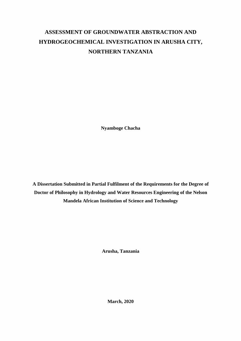
ABSTRACT
In this work geological and hydrogeochemical data, radioisotopes and stable isotopes, and
groundwater hydrographs were used to assess the groundwater abstraction trends and
hydrogeochemical characteristics of Arusha wellfield in Arusha city. Groundwater salinity in
terms of conductivity (EC) was also used to delineate salinity occurrence and distribution in
different parts of Tanzania including Arusha where this study was carried out. The
hydrogeochemical results revealed Na-K-HCO3 water type. Water-rock interaction seems to
be the main process determining the groundwater chemistry in the study area. The analysis
of geological sections showed two potential aquifers, volcanic sediment and
weathered/fractured both of which yield water with high fluoride. Eighty two (82) percent of
the analyzed groundwater samples indicated fluoride concentrations higher than WHO
guidelines and Tanzanian drinking water standards (1.5 mg/l). Groundwater hydrographs
indicated significant groundwater depletion. Water level decline of about 1.0 m/year and
discharges reduction of 10 to 57% were observed from the year 2000 to 2017. The
radiocarbon isotope signatures showed that groundwater with mean age of 1400 years BP to
modern was being abstracted from the wellfield. Recently recharged water was also
evidenced by high 14
C activities (98.1±7.9 pMC) observed in spring water. Both groundwater
hydrographs and isotope signatures suggest that the Arusha wellfield is already stressed due
to groundwater over-abstraction. Through groundwater salinity mapping, it was revealed that
generally Arusha has fresh groundwater but with relatively high electric conductivity (1000-
2000 µS/cm). The high salinity levels are partly due to dissolution of trona (evaporate
mineral) commonly found in the East African Rift System. It was further revealed that lack of
reliable hydrogeological information including interaction between surface water and
groundwater hinders water resources management efforts particularly issuance of water use
permit. Based on the findings of this study, it is recommended to carry out groundwater flow
patterns modelling to show how unregulated drilling affects the deep wells currently
depletion problem.
ii
DECLARATION
I, Nyamboge Chacha Makuri do hereby declare to the Senate of Nelson Mandela African
Institution of Science and Technology that this dissertation is my own original work and that
it has neither been submitted nor being concurrently submitted for degree award in any other
institution.
_____________________________________ ________________
Nyamboge Chacha Date
The above declaration is confirmed
Alfred N. N. Muzuka
Name of Supervisor (Posthumous)
Karoli N. Njau
________________________________________ _________________
Name and signature of supervisor Date
George V. Lugomela
_____________________________________ _________________
Name and signature of supervisor Date

iii
COPYRIGHT
This dissertation is copyright material protected under the Berne Convention, the Copyright
Act of 1999 and other international and national enactments, in that behalf, on intellectual
property. It must not be reproduced by any means, in full or in part, except for short extracts
in fair dealing; for researcher private study, critical scholarly review or discourse with an
acknowledgement, without the written permission of the office of Deputy Vice Chancellor
for Academics, Research and Innovations, on behalf of both the author and the Nelson
Mandela African Institution of Science and Technology.
iv
CERTIFIATION
This is to certify that the dissertation entitled, ―Assessment of groundwater abstraction and
hydrogeochemical investigation for sustainable water resources utilization in Arusha City,
Northern Tanzania ‖ submitted by Nyamboge Chacha Makuri (P111/T.13) in partial
fulfilment of the requirements for the award of Doctor of Philosophy in Hydrology and Water
Resources Engineering (HWRE) of Nelson Mandela African Institution of Science and
Technology (NM-AIST), Tanzania is an authentic work carried out by him under my
guidance.
Alfred N. N. Muzuka
Name of Supervisor (Posthumous)
Karoli N. Njau
_______________________________________ _________________
Name and signature of Supervisor Date
George V. Lugomela
_______________________________________ _________________
Name and signature of Supervisor Date

v
ACKNOWLEDGEMENT
This study was made possible because of enormous contributions from various individuals
and institutions within and outside Tanzania. Their contributions are highly appreciated and
valued. I would like to specifically recognize all those whose contributions have been
significant to my work.
I wish to appreciate a three years financial supports which were provided by the Government
of Tanzania through Commission for Science and Technology (COSTECH).
I am extremely indebted to my supervisors; the late Prof. Alfred N. N. Muzuka, Prof. Karoli
N. Njau and Dr. Lugomela V. George for their enthusiasm support and kind guidance
throughout my research period. The late Prof. Alfred Muzuka may his soul rest in eternal
peace and I will always remember his words of encouragement and tirelessly experience
sharing for making this study possible, Amen.
My sincere gratitude is extended to Dr. Revocatus Machunda, the Dean of the School of
Materials, Energy, Water and Environmental Sciences (MEWES and all members of staff in
the Department of Water and Environmental Science and Engineering (WESE) and entire
NM-AIST community for their advice and encouragement.
I am grateful to the Management of Arusha Urban Water supply and Sanitation Authority
(AUWSA) for allowing me to access their production boreholes for my work. I also thank all
AUWSA technical staff who tirelessly supported me during field work, namely; Eng. Fabian
Maganga, Eng. Ismail Mohamed, Messrs Respecious Mosha, Oswald Mpombo, Richard M.
Laizer, Dickson Ringo and Ackley Michael Mrema. I also thank Mr. Daniel Soka from
Arusha City Council for his kind assistance during data collection.
My sincere thanks also goes to laboratory scientists and technicians of NM-AIST (Messrs.
Paulo Sanka, Justine Lwekoramu and Wilson Mahene), Messrs Aldo Ndimbo and Ramadhan
Mburume from Ardhi University, Mr. Edwin Gowel from Southern and Eastern African
Mineral Centre (SEAMIC) for their technical advice and assistance during chemical analyses
of water samples. Mr. Reginald Tesha is thanked for his assistance during data collection and
Geostatistical analysis.
Sincere appreciations are extended to Richard Heemskerk (Laboratory Manager), Phyllis
Diebolt, Darlene Bridge and Lois Graham of Environmental Isotope Laboratory, University

vi
of Waterloo, Canada for handling radioisotopes analyses of water samples collected from
Tanzania. Also I extend my appreciation to Elvira Delgado, Emily Schick of UC Davis Stable
Isotope Facility, USA for the analyses of stable isotopes.
I owe special thanks to my colleagues and friends, Messrs Edikafubeni Makoba, Paschal
Chrisogoni and Lucas Ernest, Dr. Canute Hyandye, Dr. Talam E. Kibona, Dr. Eliapenda
Elisante, Dr. Anthony Funga and Dr. Ceven Shemsanga at the Nelson Mandela African
Institution of Science and Technology for their contribution and encouragement towards
fulfilling my work.
Special thanks go to Ardhi University community for granting me permission to pursue my
PhD programme. I wish to thank Prof. Idrissa B. Mshoro (former VC), Prof. Gabriel
Kassenga (DVC-AA), and Dr. Joseph V. Ngowi, former Dean, School of Environmental
Science and Technology (SEST) for their encouragement during my study.
Last but not least, I am greatly indebted to my parents (John Chacha Makuri and Joyce John)
for their hard work and sacrifices they made to fulfil their ambition of educating me. I further
appreciate the support from my wife (Christina Nashon) and children (Makuri, Rhobi, Esta
and Joyce), brothers and sisters.

vii
DEDICATION
This work is dedicated to my; parents (John C. Makuri and Joyce John), wife (Christina
Nashon), Children (Makuri, Rhobi, Esta and Joyce) and the rest of family members.

viii
TABLE OF CONTENTS
ABSTRACT ................................................................................................................................ i
DECLARATION ....................................................................................................................... ii
COPYRIGHT ........................................................................................................................... iii
CERTIFIATION ....................................................................................................................... iv
ACKNOWLEDGEMENT ......................................................................................................... v
DEDICATION ......................................................................................................................... vii
LIST OF TABLES ................................................................................................................. xiii
LIST OF FIGURES ................................................................................................................ xiv
LIST OF APPENDICES ........................................................................................................ xvii
LIST OF ABBREVIATIONS AND SYMBOLS ................................................................ xviii
CHAPTER ONE ........................................................................................................................ 1
INTRODUCTION ..................................................................................................................... 1
1.1 Background of the problem ............................................................................................. 1
1.2 Statement of the problem ................................................................................................. 4
1.3 Rationale of the study ...................................................................................................... 5
1.4 Objectives ........................................................................................................................ 5
1.4.1 General objective ...................................................................................................... 5
1.4.2 Specific objectives .................................................................................................... 5
1.5 Research questions ........................................................................................................... 6
1.6 Significance of the study .................................................................................................. 6
1.7 Delineation of the study ................................................................................................... 6
CHAPTER TWO ....................................................................................................................... 7
GROUNDWATER SALINITY OCCURRENCE AND DISTRIBUTION IN TANZANIA ... 7
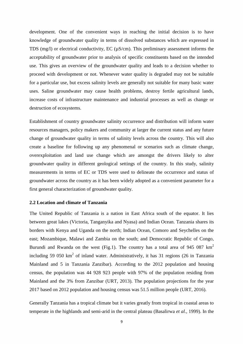
2.1 Introduction ...................................................................................................................... 8
ix
2.2 Location and climate of Tanzania .................................................................................... 9
2.3 Geology and hydrogeology ............................................................................................ 12
2.4 Origin of groundwater salinity ....................................................................................... 13
2.5 Study approach............................................................................................................... 14
2.6 Results and discussion ................................................................................................... 14
2.7 Summary and conclusions ............................................................................................. 23
CHAPTER THREE ................................................................................................................. 24
HYDROGEOCHEMICAL CHARACTERISTICS AND SPATIAL DISTRIBUTION OF
GROUNDWATER QUALITY IN ARUSHA WELL FIELDS, NORTHERN TANZANIA1 24
Abstract .................................................................................................................................... 24
3.1 Introduction .................................................................................................................... 25
3.2 Study area....................................................................................................................... 27
3.2.1 Location .................................................................................................................. 27
3.2.2 Climatic characteristics ........................................................................................... 27
3.2.3 Geological and hydrogeological settings ................................................................ 30
3.3 Materials and methods ................................................................................................... 34
3.3.1 Field work and groundwater sampling ................................................................... 34
3.3.2 Laboratory analyses ................................................................................................ 36
3.3.3 Geostatistical analysis ............................................................................................. 36
3.3.4 Piper diagram .......................................................................................................... 37
3.4 Results ............................................................................................................................ 37
3.4.1 Variation in physical-chemical properties .............................................................. 37
3.4.2 Major cations and anions ........................................................................................ 40
3.4.3 Trace elements (Fe and Mn) ................................................................................... 43
3.4.4 Multivariate analysis ............................................................................................... 43
x
3.5 Discussion ...................................................................................................................... 45
3.5.1 Groundwater chemistry ........................................................................................... 45
3.5.2 Fluoride ................................................................................................................... 49
3.5.3 Spatial distributions of nitrate, sulphate and chloride ............................................. 52
3.6 Conclusions .................................................................................................................... 53
CHAPTER FOUR .................................................................................................................... 54
GROUNDWATER ABSTRACTION AND AQUIFER SUSTAINABILITY IN ARUSHA
WELLFIELD ........................................................................................................................... 54
Abstract .................................................................................................................................... 54
4.1 Introduction .................................................................................................................... 55
4.2 Materials and Methods ................................................................................................... 56
4.2.1 Mapping of wells .................................................................................................... 56
4.2.2 Well discharge measurements................................................................................. 59
4.2.3 Water level measurements ...................................................................................... 59
4.2.4 Groundwater recharge estimation ........................................................................... 59
4.3 Results ............................................................................................................................ 60
4.3.1 Mapping of wells .................................................................................................... 60
4.3.2 Well discharge trend ............................................................................................... 60
4.3.3 Water level trend ..................................................................................................... 61
4.3.4 Groundwater abstraction ......................................................................................... 68
4.3.5 Current water demand ............................................................................................. 72
4.3.6 Groundwater recharge ............................................................................................. 73
4.4 Discussion and Conclusion ............................................................................................ 75
4.4.1 Groundwater depletion............................................................................................ 75
4.4.2 Groundwater recharge ............................................................................................. 77
xi
4.4.3 Groundwater abstraction and its impact ................................................................. 80
4.5 Conclusion ..................................................................................................................... 82
CHAPTER FIVE ..................................................................................................................... 84
GROUNDWATER AGE DATING AND RECHARGE MECHANISM OF ARUSHA
AQUIFER, NORTHERN TANZANIA: APPLICATION OF RADIOISOTOPE AND
STABLE ISOTOPE TECHNIQUES2...................................................................................... 84
Abstract .................................................................................................................................... 84
5.1 Introduction .................................................................................................................... 85
5.2 Materials and methods ................................................................................................... 88
5.2.1 Field work and groundwater sampling ................................................................... 88
5.2.2 Laboratory analyses ................................................................................................ 90
5.2.3 Groundwater age dating and 14
C correction methods ............................................. 91
5.3 Results ............................................................................................................................ 92
5.3.1 Stable isotopes and tritium ...................................................................................... 92
5.3.2 14
C and 13
C of Dissolved inorganic carbon (DIC) .................................................. 95
5.4 Discussion ...................................................................................................................... 99
5.4.1 Moisture source ....................................................................................................... 99
5.4.2 Groundwater recharge ............................................................................................. 99
5.4.3 Groundwater exploitation ..................................................................................... 101
5.5 Conclusions .................................................................................................................. 104
CHAPTER SIX ...................................................................................................................... 105
GENERAL DISCUSSION, CONCLUSION AND RECOMMENDATIONS ..................... 105
6.1 General discussion ....................................................................................................... 105
6.2 Conclusion ................................................................................................................... 109
6.3 Recommendations ........................................................................................................ 110

xii
REFERENCES ...................................................................................................................... 113
APPENDICES ....................................................................................................................... 132
RESEARCH OUTPUT .......................................................................................................... 158
Output 1: Published Papers ................................................................................................ 159
Output 2: Poster presentation ............................................................................................. 160
xiii
LIST OF TABLES
Table 1: Statistical summary of borehole hydrogeological details and electric conductivity . 15
Table 2: Classification of groundwater salinity in Tanzania ................................................... 16
Table 3: Groundwater conductivities reported in different parts of Tanzania ......................... 19
Table 4: Groundwater chemistry in the study area .................................................................. 38
Table 5: Pearson correlation matrix for samples from well water ........................................... 47
Table 6: Pearson correlation matrix for samples from spring water ........................................ 48
Table 7: One way ANOVA, Single factor results comparing spring and well waters ............ 48
Table 8: One way ANOVA, Single factor results comparing water clusters .......................... 48
Table 9: Well construction details indicating position of the screens ..................................... 50
Table 10: Statistical summary of well discharge from 2000 to 2016 in the study area ........... 62
Table 11: Groundwater abstraction (estimated) for domestic use at household level ............. 69
Table 12: Groundwater abstraction (estimated) for commercial use in Arusha city ............... 70
Table 13: Summary of estimated groundwater abstraction from existing private wells ......... 70
Table 14: Groundwater abstraction (metered water) for public water supply in Arusha city . 71
Table 15: Urban area water requirements (l/c/d) ..................................................................... 72
Table 16: Water level trends in the study area ......................................................................... 87
Table 17: Well discharge trends over time in the study area ................................................... 87
Table 18: Mean and Standard deviation of water used for calibration .................................... 90
Table 19: Physical-chemical and isotopic characteristics of groundwater in the study area ... 94
Table 20: Groundwater 14
C ages rounded to the nearest 102 years .......................................... 97

xiv
LIST OF FIGURES
Figure 1: Tanzania map showing location, regional administrative boundary and major water
bodies ..................................................................................................................... 11
Figure 2: Saline groundwater occurrence and distribution in Tanzanian (source: data
compliled from boreholes drilled across the country by Ministry of water and
irrigation, 2013-2016) ............................................................................................ 17
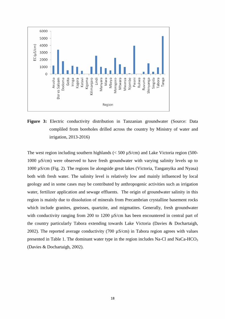
Figure 3: Electric conductivity distribution in Tanzanian groundwater (Source: Data
compliled from boreholes drilled across the country by Ministry of water and
irrigation, 2013-2016) ............................................................................................ 18
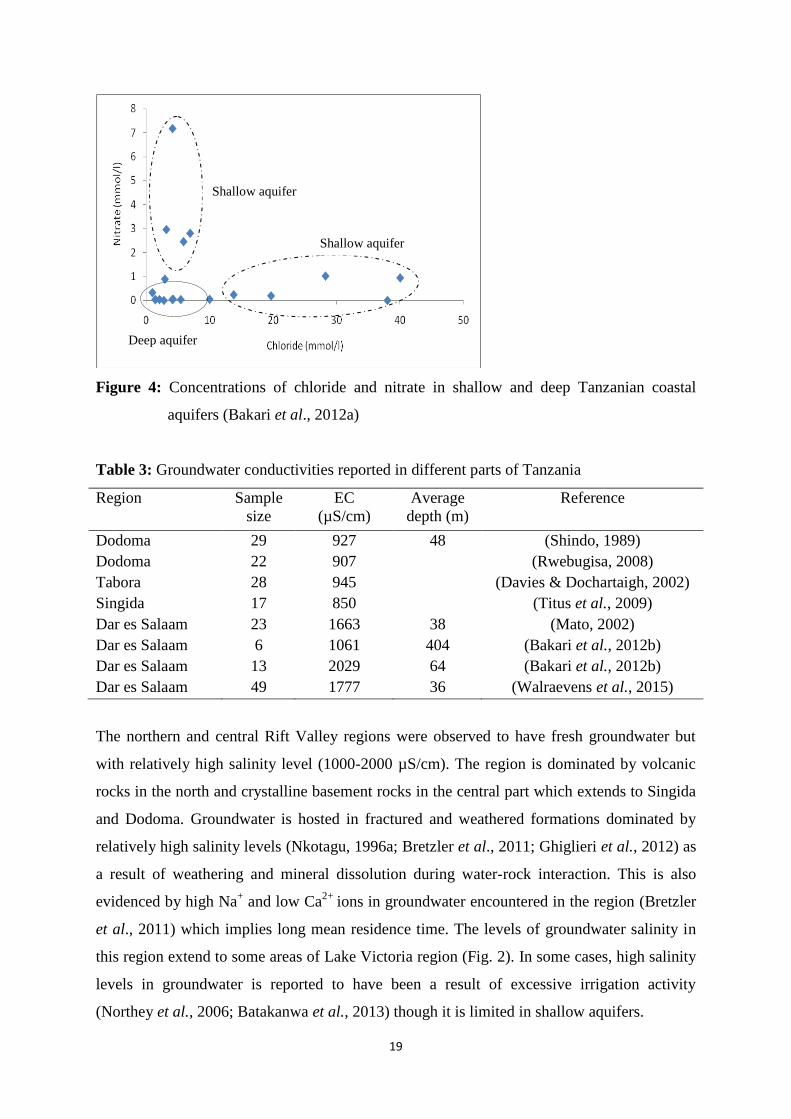
Figure 4: Concentrations of chloride and nitrate in shallow and deep Tanzanian coastal
aquifers (Bakari et al., 2012a)................................................................................ 19
Figure 5: Groundwater salinity variation with depth in coastal aquifers (a) chloride (b) nitrate
(c) condcuctivity (Bakari et al., 2012a) ................................................................. 21
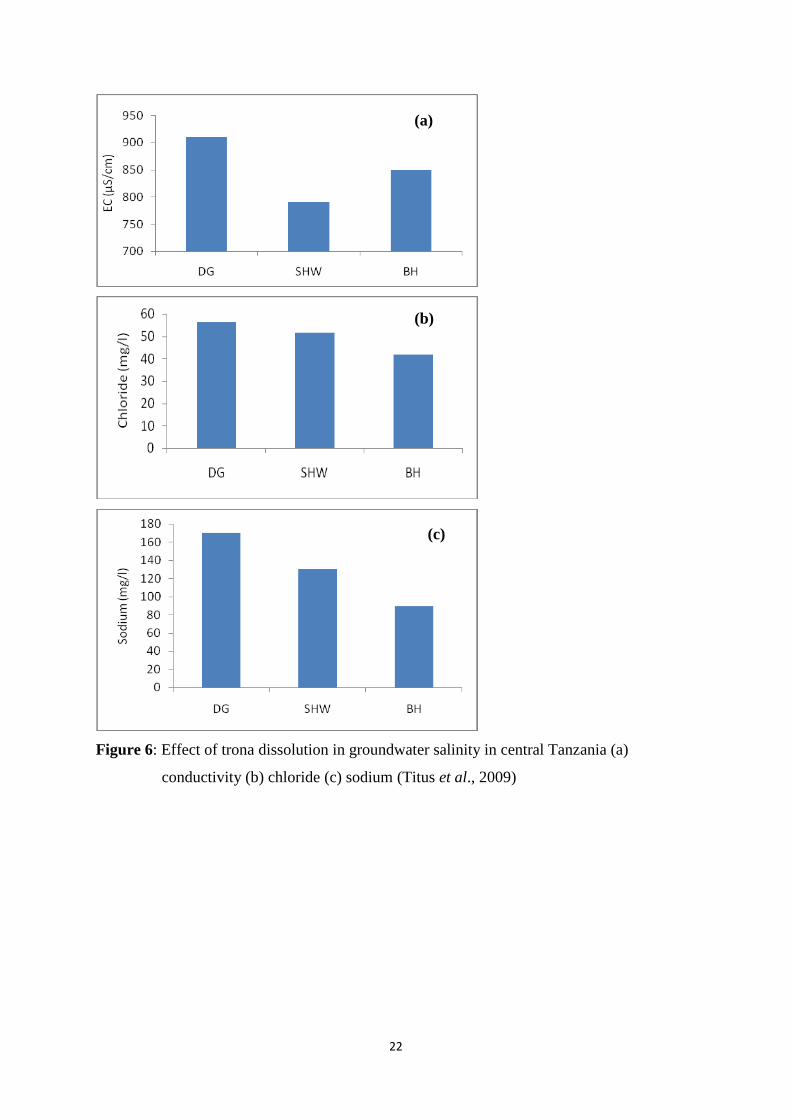
Figure 6: Effect of trona dissolution in groundwater salinity in central Tanzania (a)
conductivity (b) chloride (c) sodium (Titus et al., 2009) ....................................... 22
Figure 7: Location of the study area ...................................................................................... 29
Figure 8: Bimodal rainfall pattern in Northern Tanzania. A, B, C and D represent Arusha
Airport, Arusha Maji, Tengeru and Kilimanjaro International Airport MET
stations respectively (TMA, 2013) ........................................................................ 30
Figure 9: Hydrogeological map showing location of sampling sites (AA.VV., 1983) ......... 33
Figure 10: Geological cross section C-C´ from the steep slopes of Mt. Meru towards the foot
of the Mountain. ..................................................................................................... 34
Figure 11: Geological section A-A´ derived from well lithology logs in the study area ......... 35
Figure 12: Piper diagram for chemical composition of groundwater in the study area .......... 40
Figure 13: Scatter plot Sulphate and Chloride ......................................................................... 42
xv
Figure 14: Phosphate variations with well depth ..................................................................... 42
Figure 15: Dendrogram for groundwater hydrogeochemical data from 45 sampling sites ..... 44
Figure 16: Comparison of means of selected major ions in spring and well waters ............... 46
Figure 17: Comparison of means of selected major ions for different water clusters ............. 51
Figure 18: Groundwater development in Arusha wellfield ..................................................... 58
Figure 19: Groundwater hydrographs for Sakina borehole ..................................................... 63
Figure 20: Groundwater hydrographs for Kiranyi borehole .................................................... 63
Figure 21: Groundwater hydrographs for Lorovani bondeni borehole .................................... 64
Figure 22: Groundwater hydrographs for Lorovani yard borehole ......................................... 64
Figure 23: Groundwater hydrographs for Sanawari P/S borehole ........................................... 65
Figure 24: Groundwater hydrographs for Old Sanawari borehole .......................................... 65
Figure 25: Groundwater hydrographs for Moivo II borehole .................................................. 66
Figure 26: Groundwater hydrographs for Ilboru borehole ...................................................... 66
Figure 27: Groundwater hydrographs for Oltulelei borehole .................................................. 67
Figure 28: Groundwater hydrographs for EMCO borehole ..................................................... 67
Figure 29: Oltulelei borehole water level changes over time .................................................. 68
Figure 30: Sanawari P/S borehole water level changes over time .......................................... 68
Figure 31: Potential groundwater recharge zone in the study area .......................................... 74
Figure 32: Scatter plot showing association between discharge with well depth .................... 76
Figure 33: Average maximum temperature trend from 1973 to 2013, Arusha Airport MET
station (TMA, 2013) .............................................................................................. 77
Figure 34: Average maximum temperature trend from 1973 to 2013, Kilimanjaro
International Airport MET station (TMA, 2013) ................................................... 78
Figure 35: Annual rainfall trend from 1955 to 2013, Arusha Airport MET station (TMA,
2013) ...................................................................................................................... 79
xvi
Figure 36: Annual rainfall trend from 1955 to 2013, Arusha Maji MET station (TMA, 2013)
................................................................................................................................ 79
Figure 37: Annual rainfall trend from 1955 to 2013, Tengeru MET station (TMA, 2013) ..... 80
Figure 38: Annual rainfall trend from 1955 to 2013, Kilimanjaro International Airport MET
station (TMA, 2013) .............................................................................................. 80
Figure 39: Hydrogeological map showing location of sampling sites (AA.VV., 1983) ......... 89
Figure 40: Stable isotope signatures of groundwater in the study area ................................... 93
Figure 41: Scatter plot for δ13
C with (a) bicarbonate and (b) electrical conductivity in water
samples ................................................................................................................... 96
Figure 42: Scatter plot for 14
C activity associated with (a) altitude and (b) well depth .......... 98
Figure 43: Relationship between stable isotopes and 14
C activity in water samples: (a)
hydrogen, and (b) oxygen isotopes. The wells inside the ellipse shape are located
in alluvial deposits. .............................................................................................. 100
Figure 44: Seasonal variations of spring flows (S04 and S07) characterized by modern
groundwater. Source: The data were compiled from daily flow measurements
conducted by Arusha Urban Water Supply and Sanitation Authority. The flow is
measured by means of a broad-crested weir with a rectangular control station. . 103

xvii
LIST OF APPENDICES
Appendix 1: Groundwater quality spatial distribution........................................................... 132
Appendix 2: Well lithology logs and completion details...................................................... 136
Appendix 3: Well lithology logs ............................................................................................ 138
Appendix 4: Stable isotopes analysis procedure .................................................................... 155
Appendix 5: Radiocarbon Analytical procedure .................................................................... 156
Appendix 6: Principal data commonly required for developing a management strategy ...... 157
xviii
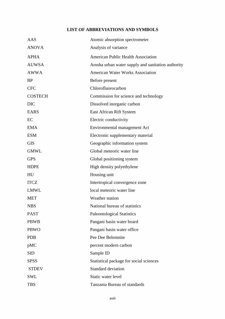
LIST OF ABBREVIATIONS AND SYMBOLS
AAS Atomic absorption spectrometer
ANOVA Analysis of variance
APHA American Public Health Association
AUWSA Arusha urban water supply and sanitation authority
AWWA American Water Works Association
BP Before present
CFC Chlorofluorocarbon
COSTECH Commission for science and technology
DIC Dissolved inorganic carbon
EARS East African Rift System
EC Electric conductivity
EMA Environmental management Act
ESM Electronic supplementary material
GIS Geographic information system
GMWL Global meteoric water line
GPS Global positioning system
HDPE High density polyethylene
HU Housing unit
ITCZ Intertropical convergence zone
LMWL local meteoric water line
MET Weather station
NBS National bureau of statistics
PAST Paleontological Statistics
PBWB Pangani basin water board
PBWO Pangani basin water office
PDB Pee Dee Belemnite
pMC percent modern carbon
SID Sample ID
SPSS Statistical package for social sciences
STDEV Standard deviation
SWL Static water level
TBS Tanzania Bureau of standards
xix
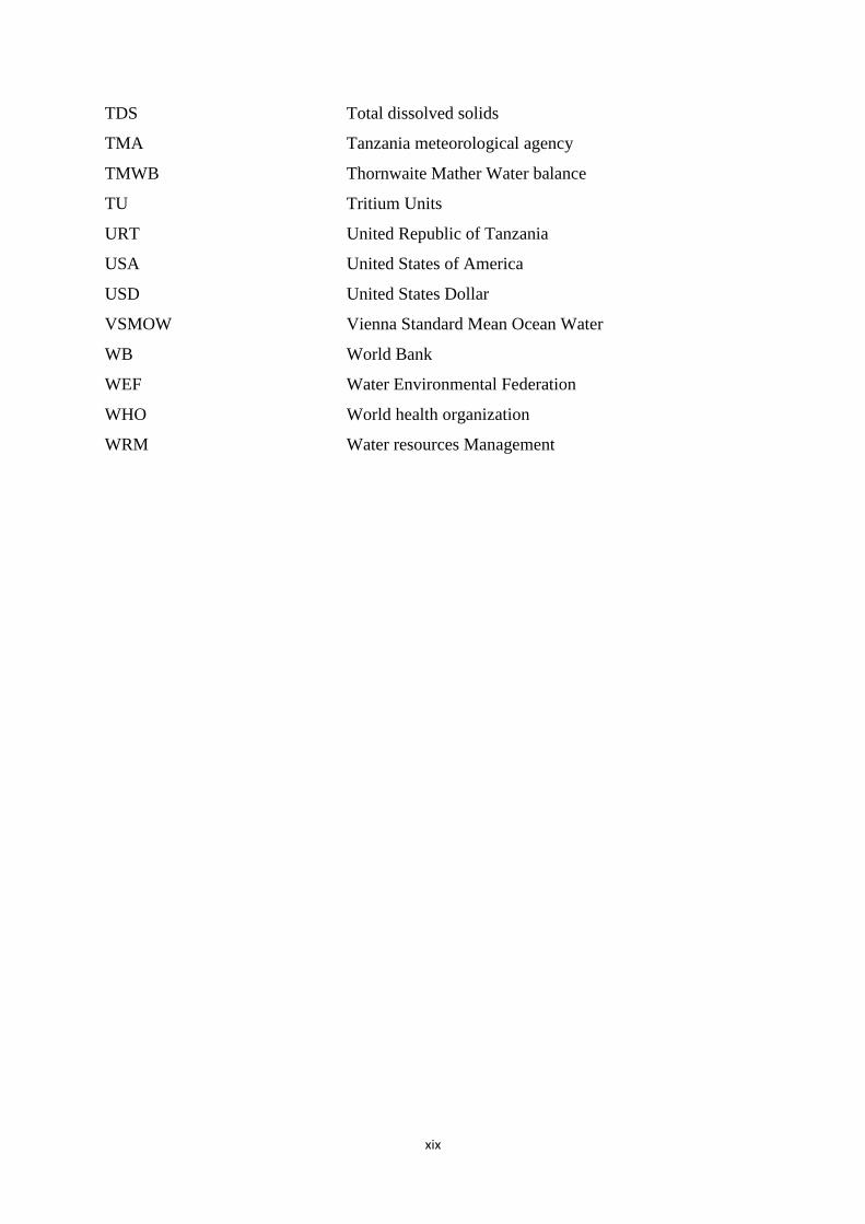
TDS Total dissolved solids
TMA Tanzania meteorological agency
TMWB Thornwaite Mather Water balance
TU Tritium Units
URT United Republic of Tanzania
USA United States of America
USD United States Dollar
VSMOW Vienna Standard Mean Ocean Water
WB World Bank
WEF Water Environmental Federation
WHO World health organization
WRM Water resources Management

1
CHAPTER ONE
INTRODUCTION
1.1 Background of the problem
Fresh groundwater which is about 0.61% of the world‘s water resources and 98% of fresh
water resources (ice caps and glaciers excluded) has a vital role for socioeconomic
development and ecosystem integrity (Carpenter, Fisher, Grimm & Kitchell, 1992; Foster &
Chilton, 2003). Under the stressed and continuously changing global climate mainly caused
by human activities, groundwater reserve seems to be the only reliable source of water supply
in terms of quality and availability at any one time (Aeschbach-Hertig & Gleeson, 2012;
Franco et al., 2018). It‘s well known that larger cities in the world and intensive irrigated
agriculture in semi-arid and humid regions depend mostly on groundwater as the main source
of water supply (Konikow & Kendy, 2005; Doell et al., 2014). This is because surface water
is highly vulnerable to climate change owing to prolonged drought, and quality deterioration
due to anthropogenic influence (Foster & Chilton, 2003). Also fresh groundwater has been
estimated to be about 100 times more plentiful than fresh surface water (Fitts, 2002). Large
groundwater abstraction is reported in both developed and developing countries such as USA,
Europe, China, India Iran and Pakistan. The estimated total global abstraction is
approximately 734 ±82 km3 per year (Konikow & Kendy, 2005; Wada et al., 2010). Despite
the economic and ecological value of groundwater, its reserves are declining from local,
regional to global scales.
Groundwater depletion has been caused by intensive abstraction due to increasing water
demand as a result of population growth and socioeconomic development which is
accompanied by industrialization (Konikow & Kendy, 2005; Giordano, 2009; Aeschbach-
Hertig & Gleeson, 2012; Bakari et al., 2012a; Famiglietti, 2014; Russo & Lall, 2017).
Climate change has been reported to intensify the problem in some regions of the world
including Africa and Brazil (Döll, 2009; Russo & Lall, 2017). Some of the groundwater
depletion effects include decreasing well yields, rising pumping costs, water quality
deterioration and damaging of aquatic ecosystem (Konikow & Kendy, 2005; Sishodia et al.,
2017). Since the problem has been a global issue, a better understanding of the status of
different exploited aquifers and appropriate management solutions worldwide is inevitable.
Otherwise the problem of water scarcity, food security and sea level rise which have been

2
reported as some of the groundwater depletion effects (Aeschbach-Hertig & Gleeson, 2012)
will spread to areas that could have avoided the risk by taking prior measures.
Although Tanzania has many surface water resources such as large fresh lakes and rivers,
groundwater has been playing crucial role in domestic, industrial and irrigation supplies. The
rural areas and major towns and municipalities in central and northern regions which are
characterized by semi-arid to humid climate depend largely on groundwater abstraction as the
main source of water supply (Kashaigili, 2010; Taylor et al., 2013). It is estimated that about
50% of total groundwater abstracted in the country is used to supply rural areas mainly for
domestic purpose whereas, 10% is being consumed in urban areas (Kashaigili, 2010). Arusha,
where the current study was conducted, is one of the regions which depend largely on
groundwater as the main source of water supply. Others include Dodoma, Singida and
Kilimanjaro (Kashaigili, 2010). In Arusha city, groundwater contributes more than 80% of
the water supply for domestic and other uses such as industrial and agriculture (AUWSA,
2014).
Despite the lack of reliable information on the extent of groundwater abstraction, there is
evidence of groundwater depletion in the study area. This includes decline of water levels and
subsequently yields reduction in wells that have been functioning for more than 20 years
(Ong‘or & Long-cang, 2007; GITEC & WEMA, 2011). Moreover, an inventory conducted
by Pangani Basin Water Office (PBWO) in 2013 revealed more than 400 wells in the study
area were drilled without groundwater permit from water resources management authority.
This suggests that groundwater abstraction in the area is not adequately controlled to meet the
needs of present and future use (Kashaigili, 2010; Van Camp et al., 2014). Therefore, the
ongoing groundwater abstraction in the study area needs a thorough investigation to clearly
document the current status of the wellfield and provide a better option for future
groundwater management.
Groundwater quality is likely to change due to depletion or over-abstraction effect (Konikow
& Kendy, 2005). This happens when there is induced leakage from the land surface,
confining layers or adjacent aquifers that contain water of inferior quality due to over-
pumping. The problem of over-abstraction of groundwater resource has been and will keep
increasing as a result of unregulated groundwater development in the study area and all over
the country (Custodio, 2002; Reddy, 2005). Fluoride is among critical natural contaminants
in groundwater resource particularly in northern Tanzania. In close proximity, its

3
concentrations vary from one source of water to another (e.g., spring and well) depending on
the mineralogical composition of the area. According to AUWSA personal communication
(2015) several boreholes have been abandoned due to increase in fluoride concentrations
exceeding 10 mg/l which is beyond both Tanzanian drinking water standards and WHO
guidelines (1.5 mg/l). Despite all these challenges, baseline and monitoring information on
the trends of groundwater quality in the wellfield are lacking. This necessitates the need for
undertaking hydrogeochemical investigations and establishing spatial variation of
groundwater quality in the study area for future groundwater planning and management.
Aquifer storage may be affected by a number of factors other than groundwater over-
abstraction (Custodio, 2002). Natural phenomena, such as delayed and transient effects of the
aquifer system, earth quakes, tectonic movement and climate change, have been reported in
many parts of the world with significant effect in aquifer productivity (Custodio, 2002;
Gorokhovich, 2005; Kitagawa et al., 2006; Kløve et al., 2014; Nigate et al., 2017). Due to the
complexity and dynamics of hydrogeological processes, knowledge of a particular aquifer
system including recharge mechanisms and age of abstracted groundwater is required to
inform the cause and extent of the existing problems. Such a situation leaves a number of
questions with respect to sustainability of groundwater utilization in Arusha city for present
and future water resources development and for avoidance of likely human impacts (drinking
water supply) and ecosystem impacts. Such impacts include reduced stream flows and
springs drying up and subsequent impacts on water-dependent ecosystems. Among the issues
to be addressed are whether groundwater storage depletion is caused by over-abstraction or
the aquifer system in the study area is not actively recharged.
Despite having laws and regulations governing groundwater development in Tanzania most
wells have been developed without groundwater permit (Kashaigili, 2010). Such practices
carried out by individuals and private entities are likely to threaten the sustainability of the
aquifers which is the main source of water supply in Arusha city. Because of unregulated
drilling activities in the area even the distance limits for sinking wells or boreholes as stated
in the Water Resources Management Act (2009) is not adhered to. This has probably affected
many production wells currently used for public water supply. The practice may be due to
lack of awareness to the community on the likely groundwater depletion impacts. This calls
for a comprehensive groundwater management strategy which can only be realized by

4
generating key information such as physical and chemical frameworks, hydrological and
hydrogeological setting of the wellfield (Alley et al., 1999; Appendix 6).
Drilling and development of a well to completion is a costly investment ( D 12,000) of
which many people do not afford in less developed countries like Tanzania (Kashaigili,
2010). Because of lack of groundwater quality information in a particular area one end up
wasting money in drilling a well which eventually produces water of inferior quality mostly
with high salinity levels. Salinity measurement in terms of electric conductivity (EC) can be
used to delineate the occurrence and status of groundwater as it has been widely adopted as a
convenient parameter for the first general characterization of groundwater quality. With few
available boreholes data drilled across the country and previously published works, a general
groundwater quality description is possible for informing prospective groundwater developer
in Tanzania including Arusha where this study was conducted.
1.2 Statement of the problem
In Arusha city, groundwater is contributing more than 80% of the daily water production
(~47 000 m3) for domestic and other uses such as industrial and agriculture (AUWSA, 2014).
Due to population increase the current water demand is about 93 000 m3/d which is twice the
amount supplied to the entire city by AUWSA. The situation has forced majority of the
residents to carry out individual well drilling for commercial and domestic water supply
purposes. Groundwater drilling and abstraction rates are not adequately regulated as a result
of groundwater depletion in the study area. Some of depletion indicators include decline of
water levels and subsequently yields reduction in wells that have been functioning for more
than 20 years (Ong‘or & Long-cang, 2007; GITEC & WEMA, 2011). Groundwater quality
deterioration particularly increases in fluoride concentrations exceeding 10 mg/l which is
beyond Tanzanian drinking water standards (1.5 mg/l) has been encountered in the wellfield
(AUWSA personal communication, 2015). This is probably contributed partly by
groundwater depletion whereby the effect can induce movement of water with inferior quality
from adjacent aquifers. Therefore, the quality of groundwater used by population which is not
served by AUWSA is uncertain. Also due to evidence of groundwater depletion, the status of
groundwater quality in the entire wellfield is of utmost importance for proper groundwater
management. Despite the ongoing intensive groundwater development, groundwater age and
aquifer recharge mechanism of the wellfield has not been researched. Lack of such vital
information hinders deliberation on informed planning and management decisions.
5
1.3 Rationale of the study
According to the well drilling reports from Arusha urban water supply and sanitation
authority (AUWSA), groundwater abstraction in Arusha wellfield commenced in late 1960s.
Currently, groundwater is contributing more than 80% of the daily water supply for domestic
and other uses in Arusha city (AUWSA, 2014). However, groundwater development is not
adequately controlled (Kashaigili, 2010; Van Camp et al., 2014), even the amount of
groundwater abstracted from the wellfield is not clear. For example in 2013 Pangani Basin
Water Office (PBWO) carried out and inventory which revealed more than 400 wells in the
wellfield were drilled without groundwater permit. Despite lack of reliable information on the
extent of groundwater abstraction, there is evidence of groundwater depletion in the study
area (Ong‘or & Long-cang, 2007; GITEC & WEMA, 2011). The ongoing groundwater
abstraction in the study area needs a thorough investigation to clearly document the current
status of the wellfield and provide a better option for future groundwater management.
Therefore, this study employed both field data and secondary data compiled from well
drilling reports and monitoring records obtained from government agencies to assess
groundwater abstraction trends and hydrogeochemical characteristics of Arusha wellfield for
sustainable water resources utilization.
1.4 Objectives
1.4.1 General objective
The general objective of this study was to assess groundwater abstraction trends and
hydrogeochemical characteristics of Arusha wellfield for sustainable water resources
utilization
1.4.2 Specific objectives
(i) To assess hydrogeochemical characteristics and establish groundwater quality spatial
variation in Arusha wellfield.
(ii) To assess groundwater abstraction and water level (drawdown) trends and possible
impacts from existing production wells.
(iii) To establish groundwater age and recharge mechanism for sustainable groundwater
utilization in Arusha City.

6
1.5 Research questions
(i) What are factors that influence groundwater chemistry and how does its quality varies
in the wellfield?
(ii) To what extent do aquifers in Arusha wellfield have been depleted from the ongoing
groundwater development?
(iii) What is the age of groundwater abstracted from Arusha wellfield and how does its
abstraction affects sustainability of the aquifer?
1.6 Significance of the study
Groundwater management is a complex subject which needs accurate and reliable
information including understanding of hydrogeological properties of an aquifer for informed
decisions (Aeschbach-Hertig & Gleeson, 2012). Excessive groundwater abstraction which
leads to depletion problem is becoming a global crisis and calls for better understanding of
the aquifer dynamics (Wada et al., 2010; Bakari et al., 2012a; Famiglietti, 2014). Therefore,
this study examines better options for evaluating and managing groundwater depletion in
Arusha wellfield. It is expected that findings of this study are vital and may contribute to
formulation of policies, bylaws and strategies for protection and management of the water
resources in Arusha city. Groundwater abstraction trends, spatial variation of groundwater
chemistry, age of groundwater and aquifer recharge mechanism are some of the findings from
this study which are important and necessary for proper management strategy. Through
information generated out of this study, the general public, water resources managers, policy
makers and other stakeholders can equally benefit for future planning and management
decisions. Additionally, the scientific findings of this study in most aspects establish the
bases for future research works as well as any physical chemical changes in the aquifer
systems.
1.7 Delineation of the study
Groundwater flow patterns modelling and groundwater balance in this study could be
considered for further studies to ascertain how unregulated drilling affects the deep wells
currently facing significant water level decline and subsequently discharge reduction. This
study established water abstraction trends, hydrogeochemical characteristics and age of the
groundwater in the wellfield but the interaction between adjacent aquifers and surface water
bodies is not known.

7
CHAPTER TWO
GROUNDWATER SALINITY OCCURRENCE AND DISTRIBUTION IN
TANZANIA
Abstract
Borehole data such as electric conductivity (EC), chloride, well depth, static water level
(SWL), drawdown and yield were collected from government databases and reports for
groundwater drilling projects all over the country. The data were analyzed using statistical
techniques and ArcGIS software for establishment of saline groundwater distribution across
Tanzania. Saline groundwater mapping revealed both brackish and freshwater in different
parts of the country. The brackish water is commonly found in coastal areas with average
value of conductivity ranging from 2271 to 5324 µS/cm. The elevated salinity level is mainly
contributed by seawater intrusion as a result of intensive groundwater development along the
coastal aquifers. The confined deep coastal aquifers ranging from 200 to 600 m below ground
surface are characterized by relatively low concentration of conductivity, chloride and nitrate.
This suggests that the effect of seawater intrusion is more pronounced in unconfined shallow
aquifers. The northern and central Rift Valley region was observed to have fresh groundwater
but with relatively high salinity level (1000-2000 µS/cm). The region falls within the East
African Rift System (EARS) which is dominated by volcanic and sedimentary rocks. The
origin and sources of high salinity levels are mainly weathering and mineral dissolution
processes during water-rock interaction. In addition, trona is another factor which contributes
to high salinity levels in groundwater due to leaching processes as a result of excessive
evaporation commonly found in EARS. The western part of the country as well as southern
highlands and Lake Victoria region were observed to have fresh groundwater with salinity
levels less than 1000 µS/cm. The salinity level is relatively low and mainly influenced by
local geology and in some cases may be contributed by anthropogenic activities such as
irrigation water, fertilizer application and sewage effluents.
Key words: Saline groundwater, Electric conductivity, Tanzania
8
2.1 Introduction
Groundwater plays a fundamental role in human prosperous and a wide range of
environmental services. It is the only source of water supply in arid region and supplementing
water supply in semi arid and humid regions where surface water bodies are now becoming
scarce and degraded because of the anthropogenic pollution and partly due to climate change
effects. Thus, groundwater is widely accessible and less vulnerable to quality degradation
than surface water bodies.
Fresh water supply is about 2.5% of the total global water resources and only less than 1% is
available and accessible for human needs and ecosystems (Gleick, 1993; Shiklomanov,
1998). Large part of global water resources (~97.5%) is seawater with the remaining per cent
distributed in ice caps and glaciers, groundwater, fresh lakes, soil moisture, atmosphere and
rivers. Groundwater is however, classified based on total dissolved solids (TDS) as fresh
water (0 – 1000 mg/l), brackish water (1000 – 10 000 mg/l), saline water (10 000 – 100 000
mg/l) and brine water (> 100 000 mg/l) (Van Weert et al., 2009).
The occurrence of groundwater with different salinity levels is mainly governed by
geological formations and mineralogical composition of the parent rocks. However, the
quality of groundwater is not fixed in time rather it is subject to change. Some changes can be
observed more quickly and others happen very slowly and are only significant at a geological
time scale. Groundwater quality notably salinity levels may change in response to many
factors both natural and anthropogenic influences. These include land use change due to
human activities, groundwater pumping, intensive irrigation, fertilizer application,
wastewater disposal, sea level rise as a result of climate change and meteorological processes
such as evaporation and evapotranspiration.
According to Kashaigili (2010), the on-going groundwater resources development in
Tanzania is being carried out without adequate knowledge of the resource in terms of quality
and quantity due to lack of information and uncontrolled development. High costs of well
drilling and development estimated to about USD 12 000 and hydrogeochemical analysis of
about USD 20 per parameter (Kashaigili, 2010) have been a major constraint in groundwater
development particularly when the aquifer under consideration is generally degraded because
of either natural or anthropogenic drivers. It is therefore inevitable to establish baseline
information based on the scattered available data on groundwater resources to avoid spending
costs unnecessarily for already degraded or unsuitable aquifers prior embarking on actual
9
development. One of the convenient ways in reaching the initial decision is to have
knowledge of groundwater quality in terms of dissolved substances which are expressed in
TDS (mg/l) or electrical conductivity, EC (µS/cm). This preliminary assessment informs the
acceptability of groundwater prior to analysis of specific constituents based on the intended
use. This gives an overview of the groundwater quality and leads to a decision whether to
proceed with development or not. Whenever water quality is degraded may not be suitable
for a particular use, but excess salinity levels are generally not suitable for many basic water
uses. Saline groundwater may cause health problems, destroy fertile agricultural lands,
increase costs of infrastructure maintenance and industrial processes as well as change or
destruction of ecosystems.
Establishment of country groundwater salinity occurrence and distribution will inform water
resources managers, policy makers and community at larger the current status and any future
change of groundwater quality in terms of salinity levels across the country. This will also
create a baseline for following up any phenomenal or scenarios such as climate change,
overexploitation and land use change which are amongst the drivers likely to alter
groundwater quality in different geological settings of the country. In this study, salinity
measurements in terms of EC or TDS were used to delineate the occurrence and status of
groundwater across the country as it has been widely adopted as a convenient parameter for a
first general characterization of groundwater quality.
2.2 Location and climate of Tanzania
The United Republic of Tanzania is a nation in East Africa south of the equator. It lies
between great lakes (Victoria, Tanganyika and Nyasa) and Indian Ocean. Tanzania shares its
borders with Kenya and Uganda on the north; Indian Ocean, Comoro and Seychelles on the
east; Mozambique, Malawi and Zambia on the south; and Democratic Republic of Congo,
Burundi and Rwanda on the west (Fig.1). The country has a total area of 945 087 km2
including 59 050 km2 of inland water. Administratively, it has 31 regions (26 in Tanzania
Mainland and 5 in Tanzania Zanzibar). According to the 2012 population and housing
census, the population was 44 928 923 people with 97% of the population residing from
Mainland and the 3% from Zanzibar (URT, 2013). The population projections for the year
2017 based on 2012 population and housing census was 51.5 million people (URT, 2016).
Generally Tanzania has a tropical climate but it varies greatly from tropical in coastal areas to
temperate in the highlands and semi-arid in the central plateau (Basalirwa et al., 1999). In the
10
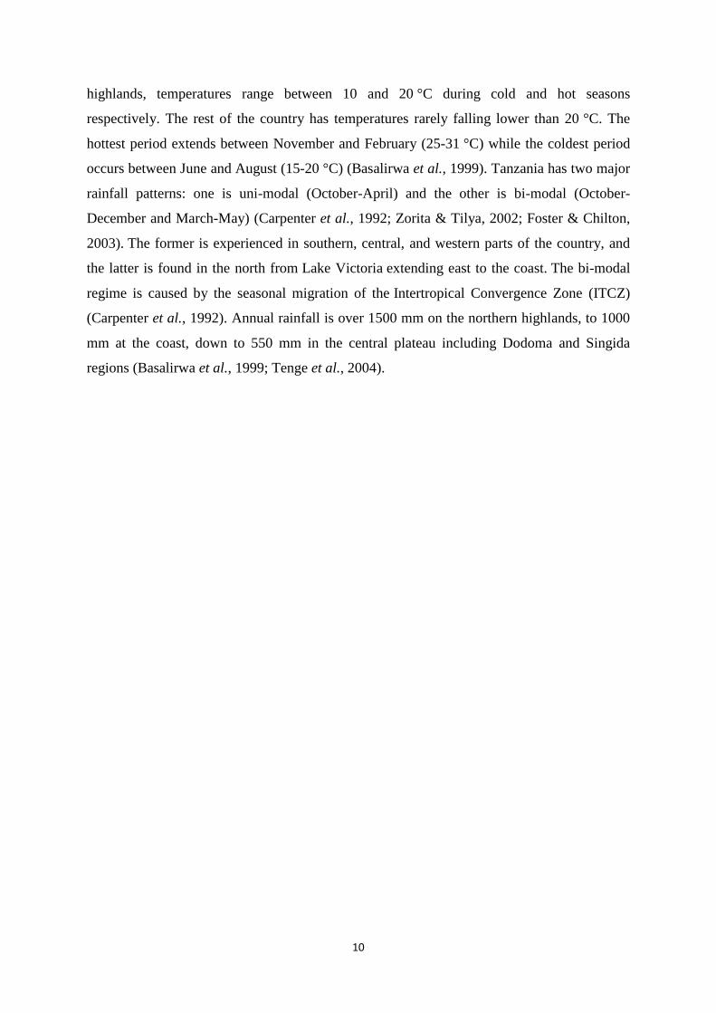
highlands, temperatures range between 10 and 20 °C during cold and hot seasons
respectively. The rest of the country has temperatures rarely falling lower than 20 °C. The
hottest period extends between November and February (25-31 °C) while the coldest period
occurs between June and August (15-20 °C) (Basalirwa et al., 1999). Tanzania has two major
rainfall patterns: one is uni-modal (October-April) and the other is bi-modal (October-
December and March-May) (Carpenter et al., 1992; Zorita & Tilya, 2002; Foster & Chilton,
2003). The former is experienced in southern, central, and western parts of the country, and
the latter is found in the north from Lake Victoria extending east to the coast. The bi-modal
regime is caused by the seasonal migration of the Intertropical Convergence Zone (ITCZ)
(Carpenter et al., 1992). Annual rainfall is over 1500 mm on the northern highlands, to 1000
mm at the coast, down to 550 mm in the central plateau including Dodoma and Singida
regions (Basalirwa et al., 1999; Tenge et al., 2004).
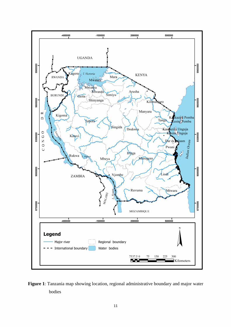
11
Figure 1: Tanzania map showing location, regional administrative boundary and major water
bodies

12
2.3 Geology and hydrogeology
The geology of Tanzania is dominated by crystalline basement rocks formed during Precambrian.
Generally, the Tanzanian geology started to form in the Precambrian, in
the Archean and Proterozoic eons, and some cases are more than 2.5 billion years ago.
Igneous and metamorphic crystalline basement rock forms the Archean Tanzania Craton,
which is surrounded by the Proterozoic Ubendian belt, Mozambique Belt and Karagwe-
Ankole Belt (Schlüter, 2008). Also Tanzania has experienced marine sedimentary rock
deposition along the coast and rift formation inland, which has produced large rift lakes. The
craton includes the vestiges of two Archean orogenic belts, the Dodoman Belt in central
Tanzania, and the Nyanzian-Kavirondian in the north. The remains of these two belts produce
lenses of sedimentary and volcanic rocks within granites and migmatite (Schlüter, 2008). The
Dodoman Belt stretches for 480 km, broadening westward and is composed of
banded quartzites, aplite, sericitic schist, pegmatite and ironstone. On the other hand, the
Nyanzian Belt is mainly acid and basic basalt, dolerite, trachyte, rhyolite and tuff in separated
zones south and east of Lake Victoria (Schlüter, 2008). The central plateau is composed of
ancient crystalline basement rocks. These are predominantly faulted and fractured
metamorphic rocks with some granite (Titus et al., 2009). Groundwater flow is restricted to
joints and fractures and is therefore limited. Groundwater is potentially more abundant in the
topmost part of the basement which has been highly weathered in places and is hence friable
and more permeable (Titus et al., 2009).
The northern and southern highland regions are parts of the major East African Rift system
which extends northwards through Kenya and Ethiopia, and which has developed over the
last 30 million years through extreme crustal tension, rift faulting and volcanic activity. The
Gregory Rift extends with a north-north-west trend through northern Tanzania and the
Western Rift extends north-west to south-east along the south-western margin of Tanzania.
The geology of the Rift zones comprises volcanic and intrusive rocks, largely of basaltic
composition, but with some rare sodic alkaline rocks and igneous carbonates (e.g. Oldoinyo
Lengai volcano). Some of the volcanic centres are active (producing new lava and ash
formations periodically) (Roberts, 2002). The dominant hydrogeological features are the
volcanic phonolitic and nephelinitic lavas, and sedimentary material of fine-grained alluvial
and lacustrine origin. Groundwater is mainly available in both fractured or faulted formation
and unconsolidated or semi-consolidated sediments (Ghiglieri et al., 2010; Ghiglieri et al.,
2012).
13
The south-eastern part of the country is composed of sedimentary rocks of various ages
(Palaeozoic to Recent), including the Karroo rocks and coal seams. The sediments are
predominantly sandstones anticipated to be originated from an estuarine deltaic environment
(Kent, 1971; Mpanda, 1997; Muhongo et al., 2000). The sediments are mixed formations,
including sandstones, mudstones and limestones. The coastal plain consists of largely
unconsolidated sediments (beach sands, dunes and salt marsh) together with some limestone
deposits (Nkotagu, 1989; Bakari et al., 2012a). Potential groundwater reserve is hosted in the
Quaternary deposits of Pleistocene to Recent periods which determine the geomorphology of
the coastal plain (Walraevens et al., 2015). Other parts of the country have not well studied
and lack relevant and reliable hydrogeological information.
2.4 Origin of groundwater salinity
Electrical conductivity (EC) is a good measure of salinity as it reflects the total dissolved
solid (TDS) in groundwater. Salinity in groundwater is contributed by various water
constituents resulting from both natural and anthropogenic processes. Some factors (in
particular anthropogenic) are only able to affect shallow aquifers while others are likely to
reach even deeper ones. Generally, groundwater salinity is controlled by salt mineral
dissolution in the aquifer matrix when water flows through subsurface environment.
Seawater intrusion occurs in coastal aquifers when fresh groundwater resources are
abstracted for human or other use and when groundwater replenishment decreases the
shallow fresh groundwater head will also decrease. This can cause up-coning of deeper saline
groundwater and an inland movement of the seawater-groundwater interface.
When irrigated water is enriched with mineral salts and applied in excess to a crop land most
likely will percolate to the shallow water table. Thus, the water vapour leaving the crops
during this process is almost without dissolved solids, thus much less mineralized than the
irrigation water supplied. Consequently, a residue of relatively mineralized water is left in the
soil. From there it may adsorb to the soil matrix, drain to the surface water system or
percolate below the root zone. In a way it may reach an aquifer and contribute to a
progressive increase in salinity of its groundwater. Similarly, evaporation process especially
in semi-arid or arid climate may affect shallow aquifers. This happens when climatic
conditions favour evaporation (or evapotranspiration through plants) while flushing of
accumulated salts is absent or only weak. Anthropogenic pollutants such as domestic and
industrial effluents, residues from fertilizer applications may enter the groundwater system
14
and contribute to increased salinity. Groundwater salinization effects of these processes will
be rather localized.
2.5 Study approach
The information used in this study was collected from government databases and reports for
groundwater drilling projects all over the country. The collected data for processing and
interpretation included location name, electric conductivity (EC), well depth, static water
level (SWL), drawdown and yield. In addition, previous published works on groundwater
chemistry were compiled across the country though some regions lacked information because
no studies have been carried out so far. The information compiled from literature made a
significant contribution to this study especially interpretation of the salinity origin for
different aquifers. Statistical analysis were performed for EC and other related parameters to
infer its level of occurrence and distribution across the country. Finally the spatial distribution
of salinity levels was plotted on the map of Tanzania using ArcGIS 10.3 software.
2.6 Results and discussion
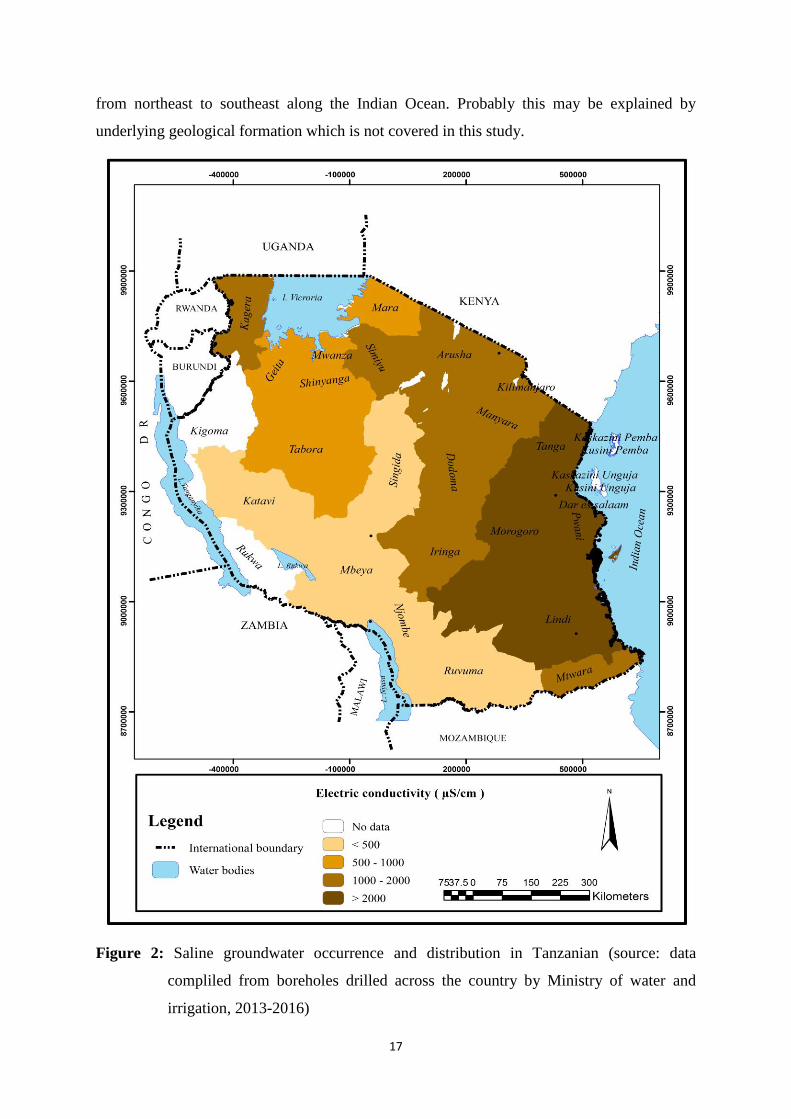
Groundwater salinity mapping revealed both brackish and freshwater occurrence across the
country (Table 1). In this study, four regions have been established based on salinity levels.
These include, southern highlands and western region (< 500 µS/cm), Lake Victoria region
(500-1000 µS/cm), Northern and central rift region (1000-2000 µS/cm) and coastal region (>
2000 µS/cm) (Table 2 and Fig. 2). The occurrence and distribution of groundwater salinity is
mainly controlled by geology of the area and anthropogenic influence (Mjemah, 2007;
Nkotagu, 1996a). However, the coastal areas (Tanga, Pwani, Dar es Salaam and Lindi) were
observed to have generally brackish water (Fig.3) as a result of sea water influence (Mjemah,
2007; Van Camp et al., 2014; Comte et al., 2016).
Unlike geological influence, the human activities such as irrigation, manure and fertilizer
application, domestic and industrial wastewater effluents mostly affect shallower aquifers
(Mjemah, 2007). In coastal region where the seawater intrusion is expected to be high,
anthropogenic contribution such as wastewater effluent seems to have negligible effect in
terms of salinity input due to elevated level of chloride particularly in shallow aquifers (Fig. 4
and 5a).
15
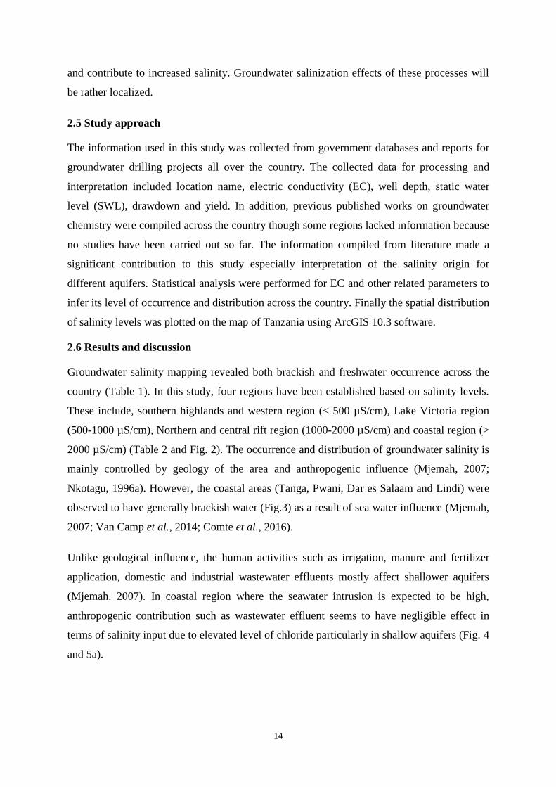
Table 1: Statistical summary of borehole hydrogeological details and electric conductivity
SN Region
Sample
size Depth (m) SWL (m b.g.l.) Yield (m3/h) EC (µS/cm)
Min. Max. Aver. Min. Max. Aver. Min. Max. Aver. Min. Max. Aver.
1 Arusha 32 42 250 124 2.15 148.50 42.21 0.80 42.60 10.02 14 3330 1205
2 Dar es Salaam 292 10 180 98 0.87 108.58 36.66 0.30 30.00 7.62 104 36000 3413
3 Dodoma 41 55 212 125 0.65 119.70 31.70 0.40 27.00 8.49 548 7080 1796
4 Geita 8 70 130 109 1.19 25.49 7.63 1.05 6.24 3.48 201 1499 531
5 Iringa 20 26 160 89 1.00 49.27 14.50 0.88 100.00 10.67 161 7730 1177
6 Kagera 12 50 220 83 0.90 51.10 11.71 0.50 15.84 6.81 196 2430 1028
7 Katavi 18 100 110 104 2.00 12.95 6.79 0.81 14.00 4.00 199 2390 457
8 Kigoma 5 60 150 105 2.89 24.10 17.14 0.60 70.00 27.08
9 Kilimanjaro 21 42 180 109 1.59 156.15 45.06 1.30 104.30 19.11 94 4835 1037
10 Lindi 33 40 150 82 0.58 64.13 16.24 0.53 38.30 10.88 70 18410 2568
11 Manyara 7 90 126 111 2.85 96.00 20.07 1.03 15.84 7.93 521 1640 1008
12 Mara 13 40 110 90 3.01 35.22 12.33 0.20 7.00 2.68 420 1454 831
13 Mbeya 26 35 120 63 1.97 43.50 14.44 0.15 22.30 5.53 102 1460 499
14 Morogoro 50 5 150 84 2.05 41.14 13.34 0.40 30.71 8.25 425 7490 2271
15 Mtwara 22 30 200 84 0.00 124.44 35.45 0.30 21.77 7.92 125 10000 1371
16 Mwanza 34 31.6 100 77 0.45 25.23 7.09 0.50 36.00 4.99 91 4970 989
17 Njombe 7 60 120 95 3.40 29.70 17.82 0.47 4.05 2.06 88 121 105
18 Pwani 105 35 210 124 0.00 145.44 41.79 0.50 46.00 6.56 9 45900 3974
19 Rukwa 6 50 76 64 1.57 13.76 8.85 0.63 24.00 7.41
20 Ruvuma 5 54 91 69 8.67 44.15 18.74 0.70 4.40 2.04 120 954 340
21 Shinyanga 24 28 124 63 2.00 27.55 6.17 0.40 24.00 6.14 100 2800 1504
22 Singida 32 36 121 67 1.93 51.65 9.42 0.40 19.80 4.71 18 1770 334
23 Tabora 22 4.9 120 59 0.40 23.70 7.12 0.11 15.84 3.57 120 4040 947
24 Tanga 27 28 145 91 0.25 60.66 12.58 1.09 42.00 13.95 526 31200 5324
Min 4.9 76 59 0.00 12.95 6.17 0.11 4.05 2.04 0.8 14 4
Max 100 250 125 8.67 156.15 45.06 44.14 104.30 78.19 548 45900 5324
Ave 42.6 148 90 1.77 63.42 18.95 2.39 35.13 11.09 184 9203 1477
Source: Data compiled from boreholes drilled across the country by Ministry of water and irrigation (2013-2016).
16
However, anthropogenic pollution has been evidenced by elevated levels of nitrate in shallow
groundwater compared to deep ones (Bakari et al., 2012a; Fig. 5b). The predominance of
brackish water with average conductivity ranging from 2271 to 5324 µS/cm indicates that
seawater has laterally intruded fresh groundwater along the coastal region (Figs. 2 and 3).
This may be due to reduced groundwater replenishment as a result of land use and land cover
change. Apart from reduced recharge, coastal area of Tanzania like many other parts of the
world is dominated by large cities including Dar es Salaam and Tanga which implies large
amount of groundwater withdraws (Van Camp et al., 2014). The main water types in the
coastal area include Na-Cl and NaCa-HCO3 (Mjemah, 2007; Bakari et al., 2012a; Mtoni et
al., 2013). Groundwater abstraction induces inland seawater movement and when mixed with
fresh groundwater the salinity level increases significantly. However, confined deep coastal
aquifers ranging from 100 to 600 m below ground surface were observed to have relatively
low levels of conductivity, chloride and nitrate (Fig. 5). This suggests that the effect of
seawater intrusion is more pronounced in unconfined shallow aquifers which have undergone
intensive development in most coastal areas of Tanzania (Mtoni et al., 2013; Van Camp et
al., 2014).
Table 2: Classification of groundwater salinity in Tanzania
Region Average EC (µS/cm) Remark
Katavi, Njombe, Ruvuma, Mbeya,
Singida < 500 Fresh water
Geita, Mara, Mwanza, Tabora,
Shinyanga 500-1000 Fresh water
Arusha, Dodoma, Iringa, Kagera,
Kilimanjaro, Manyara, Mtwara 1000-2000 Fresh water
Dar es Salaam, Lindi, Morogoro, Pwani,
Tanga >2000 Brackish water* *Brackish water is water that has more salt than freshwater, but not as much as seawater. It may result
from mixing of seawater with freshwater (occurs in brackish fossil aquifers).
Generally, groundwater in coastal region is classified as brackish water. However, Mtwara
which is in southeast coast of Tanzania (Fig. 2) was observed to have fresh groundwater with
average conductivity of 1371 µS/cm at average well depth of 84 m. The level of salinity in
groundwater of this area is far below compared to the rest of groundwater encountered along
the coastal aquifers where the maximum salinity was observed in Tanga (5324 µS/cm)
northeast of the country. A consistence decrease of salinity levels was observed as one move
17
from northeast to southeast along the Indian Ocean. Probably this may be explained by
underlying geological formation which is not covered in this study.
Figure 2: Saline groundwater occurrence and distribution in Tanzanian (source: data
compliled from boreholes drilled across the country by Ministry of water and
irrigation, 2013-2016)
18
Figure 3: Electric conductivity distribution in Tanzanian groundwater (Source: Data
compliled from boreholes drilled across the country by Ministry of water and
irrigation, 2013-2016)
The west region including southern highlands (< 500 µS/cm) and Lake Victoria region (500-
1000 µS/cm) were observed to have fresh groundwater with varying salinity levels up to
1000 µS/cm (Fig. 2). The regions lie alongside great lakes (Victoria, Tanganyika and Nyasa)
both with fresh water. The salinity level is relatively low and mainly influenced by local
geology and in some cases may be contributed by anthropogenic activities such as irrigation
water, fertilizer application and sewage effluents. The origin of groundwater salinity in this
region is mainly due to dissolution of minerals from Precambrian crystalline basement rocks
which include granites, gneisses, quartzite, and migmatites. Generally, fresh groundwater
with conductivity ranging from 200 to 1200 µS/cm has been encountered in central part of
the country particularly Tabora extending towards Lake Victoria (Davies & Dochartaigh,
2002). The reported average conductivity (700 µS/cm) in Tabora region agrees with values
presented in Table 1. The dominant water type in the region includes Na-Cl and NaCa-HCO3
(Davies & Dochartaigh, 2002).
19
Figure 4: Concentrations of chloride and nitrate in shallow and deep Tanzanian coastal
aquifers (Bakari et al., 2012a)
Table 3: Groundwater conductivities reported in different parts of Tanzania
Region Sample
size
EC
(µS/cm)
Average
depth (m)
Reference
Dodoma 29 927 48 (Shindo, 1989)
Dodoma 22 907 (Rwebugisa, 2008)
Tabora 28 945 (Davies & Dochartaigh, 2002)
Singida 17 850 (Titus et al., 2009)
Dar es Salaam 23 1663 38 (Mato, 2002)
Dar es Salaam 6 1061 404 (Bakari et al., 2012b)
Dar es Salaam 13 2029 64 (Bakari et al., 2012b)
Dar es Salaam 49 1777 36 (Walraevens et al., 2015)
The northern and central Rift Valley regions were observed to have fresh groundwater but
with relatively high salinity level (1000-2000 µS/cm). The region is dominated by volcanic
rocks in the north and crystalline basement rocks in the central part which extends to Singida
and Dodoma. Groundwater is hosted in fractured and weathered formations dominated by
relatively high salinity levels (Nkotagu, 1996a; Bretzler et al., 2011; Ghiglieri et al., 2012) as
a result of weathering and mineral dissolution during water-rock interaction. This is also
evidenced by high Na+ and low Ca
2+ ions in groundwater encountered in the region (Bretzler
et al., 2011) which implies long mean residence time. The levels of groundwater salinity in
this region extend to some areas of Lake Victoria region (Fig. 2). In some cases, high salinity
levels in groundwater is reported to have been a result of excessive irrigation activity
(Northey et al., 2006; Batakanwa et al., 2013) though it is limited in shallow aquifers.
Shallow aquifer
Shallow aquifer
Deep aquifer
20
In volcanic region within the East African Rift System, trona (evaporite mineral) dissolution
is another factor which contribute to high salinity levels in groundwater due to evaporation
and leaching processes (Kaseva, 2006; Pittalis, 2010). Trona is more abundant in dark soil
and commonly found few meters below ground surface. It is also common and found at very
high levels in the East African Rift system saline lakes such as Turkana, Suguta, Baringo,
Natron and Manyara (Olaka et al., 2010) all these contribute to high salinity levels in
groundwater of this region (Apaydin, 2010; Arslan et al., 2015). High salinity levels in
shallow aquifers in areas dominated by trona has been reported in central part of Tanzania
(Fig. 6) where dugouts and shallow wells of up to 10 m deep were observed to have high
levels of conductivity, chloride and sodium ions than deep wells ( 90 m) (Titus et al., 2009).
Groundwater salinity occurrence and distribution may significantly differ within a small area
depending on the subsurface local geology. For example, some wells along the coastal
aquifers were observed to have fresh groundwater (Table 1) despite the region being
classified under saline or brackish water. Similarly, Table 3 shows previous works which
indicate occurrence of some fresh groundwater in Dar es Salaam coastal aquifers.
Therefore, this study becomes the first step toward delineation of groundwater salinity
distribution in Tanzania but more details are necessary for specific groundwater development
cases in a particular region. In view of the aforementioned scenarios together with the
ongoing intensive groundwater development in Arusha city (Ong‘or & Long-cang, 2007;
GITEC & WEMA, 2011) a more detailed investigation on groundwater hydrogeochemistry
was carried out and the results are reported in the next chapter.

21
Figure 5: Groundwater salinity variation with depth in coastal aquifers (a) chloride (b) nitrate
(c) condcuctivity (Bakari et al., 2012a)
(a)
(b)
(c)
22
Figure 6: Effect of trona dissolution in groundwater salinity in central Tanzania (a)
conductivity (b) chloride (c) sodium (Titus et al., 2009)
(a)
(c)
(b)
23
2.7 Summary and conclusions
Mapping of saline groundwater in Tanzania revealed both brackish and freshwater in
different parts of the country. The brackish water is commonly found in coastal areas from
Tanga in the north to Lindi in southeast. The salinity level in terms of average conductivity
ranged from 2271 to 5324 µS/cm (Table 1). Apart from mineral dissolution, elevated salinity
level is contributed by seawater intrusion as a result of intensive groundwater development
along the coastal aquifers in which major towns and cities are located. Contribution of
anthropogenic activities is also noticeable but becomes negligible because of high salinity
levels from seawater intrusion. However, confined deep coastal aquifers ranging from 100 to
600 m below ground surface were observed to have relatively low levels of conductivity,
chloride and nitrate compared to semi-confined and unconfined ones (Bakari et al., 2012a,
2012b). This suggests that the effect of seawater intrusion is more pronounced in unconfined
shallow aquifers which have undergone intensive groundwater development in most coastal
areas of Tanzania.
The northern and central Rift Valley region was observed to have fresh groundwater but with
relatively high salinity level (1000-2000 µS/cm). The region falls within the East African Rift
System (EARS) which is dominated by volcanic and sedimentary rocks. The origin and
sources of high salinity levels are mainly weathering and mineral dissolution processes
during water-rock interaction. This is also evidenced by high Na+ and low Ca
2+ ions in
groundwater encountered in the region. However, the broader spectrum of groundwater
hydrogeochemistry of Arusha city (study area of this work) is discussed under chapter three
(3) of this report. In addition, trona which is an evaporite mineral in the EARS is another
factor which contributes to high salinity levels in groundwater due to evaporation and
leaching processes.
The west part of the country including southern highlands and Lake Victoria region was
observed to have fresh groundwater with salinity levels less than 1000 µS/cm. The salinity
level is relatively low and mainly influenced by local geology and in some cases may be
contributed by anthropogenic activities such as irrigation water, fertilizer application and
sewage effluents. Apart from anthropogenic influence, the origin of groundwater salinity in
this region is due to dissolution of minerals from basement rocks which include granites,
gneisses, quartzite, and migmatites.
24
CHAPTER THREE
HYDROGEOCHEMICAL CHARACTERISTICS AND SPATIAL DISTRIBUTION
OF GROUNDWATER QUALITY IN ARUSHA WELL FIELDS, NORTHERN
TANZANIA1
Abstract
Arusha aquifers have been exploited intensively serving as the main source of domestic
water supply in the city. But the quality of groundwater is not clearly documented for future
planning and management. Hydrogeochemical assessment was carried out to establish
groundwater quality and its spatial distribution with the aid of geostatistical techniques.
Groundwater samples were collected and analyzed for major cations and anions using
conventional methods of water analysis. Well lithology and geological map were considered
for hydrogeological interpretation of the area. The results of piper diagram revealed Na-K-
HCO3 water type with sodium and bicarbonate ions dominating in all samples. High fluoride
concentrations and general groundwater chemistry are mainly controlled by aquifer lithology
than anthropogenic activities. The levels of anthropogenic pollution indicators such as nitrate,
chloride and sulphate in deep wells are generally low and most likely coming from natural
sources. The geological sections indicate two potential aquifers (volcanic sediment and
weathered/fractured formation) both yield water containing significant concentration of
fluoride. Eighty two (82) percent of the analyzed groundwater samples indicated fluoride
concentrations higher than WHO guidelines and Tanzanian drinking water standards (1.5
mg/l). The southern part of the study area yields groundwater of better quality for human
consumption than northern zones which is at high elevation on the foot of Mt. Meru. With
exception of fluoride the quality of groundwater in the study area is generally suitable for
drinking purpose and other socioeconomic uses.
Key words: Groundwater quality; Hydrogeochemical; Arusha
1Applied Water Science (2018) 8:118, https://doi.org/10.1007/s13201-018-0760-4

25
3.1 Introduction
Water is the most important natural resource for continued existence of any community or
ecosystem (Jha et al., 2007; Kløve et al., 2014; Gleeson et al., 2016). Most social economic
processes and functions of a particular community are largely depending on potable water
supply (Brown & Lall, 2006; Chenoweth, 2008; Komakech et al., 2012). Its vital role
necessitates the importance of understanding water resources dynamics throughout the world
for present and future use (Schmoll et al., 2006; Heathwaite, 2010; Hellar-Kihampa et al.,
2013). Due to socio-economic development, rapid population growth and increased
incidences of freshwater pollution (Schwarzenbach et al., 2010), groundwater exploitation
has increased tremendously in many parts of the world (Taylor et al., 2013; Venetsanou et
al., 2015; Cheema, 2016). Knowledge on the availability and quality of water is inevitable in
groundwater development and management programs.
The quality of groundwater is mainly governed by local geology and highly influenced by
environmental factors (Fitts, 2002). Factors such as rainfall, temperature and pH conditions
facilitate different subsurface physical chemical processes such as weathering, dissolution
and ion exchange (Gizaw, 1996). Under ideal conditions, these processes are the ones that
determine groundwater chemistry and its quality as it moves across different geological
formations (Kump et al., 2000; Olobaniyi & Owoyemi, 2006). However, apart from natural
and anthropogenic pollution sources, over-abstraction has been reported worldwide as a
threat to both groundwater quality and quantity (Changming et al., 2001; Delinom, 2008;
Wada et al., 2010). In order groundwater abstraction to be sustainable, a better understanding
of both quantity and quality of water need to be defined by applying proper management
strategies with the aid of reliable hydrogeological and hydrogeochemical data of an aquifer
(Gleeson et al., 2012). This study focused on geostatistical methods for establishing
groundwater quality spatial distribution in the study area. The use of Geographic information
system (GIS) technique has been widely adopted in proper planning and management of
groundwater resource (Dixon, 2005; Jha et al., 2007; Rahmati et al., 2015) due to its vast
capability of effective storage, spatial analysis, and presentation of graphical outputs on water
quality issues (Fenta et al., 2015; Venkatramanan et al., 2015). Hydrogeochemical data and
spatial analysis helps to understand the groundwater quality distribution and its suitability
based on available local standards and World health organization‘s (WHO) guidelines for

26
various uses. Such knowledge helps water resource managers and policy makers to properly
plan and manage the vital resource for present and future use.
The current study was conducted in a volcanic area (southern slope of Mt. Meru) located
within East African Rift System. The quality of groundwater in the rift system has been
reported in previous works particularly in the Main Ethiopian Rift whereby high levels of
fluoride, bicarbonate and sodium are a major concern due to high rate of carbon dioxide
outgassing, acid volcanic and geothermal heating (Gizaw, 1996; Bretzler et al., 2011). High
fluoride level in drinking water is a serious threat to human health specifically causing dental
fluorosis and other related diseases (Moturi et al., 2002). Such natural contaminants are not
uniform in groundwater systems rather are distributed depending on geological formation of a
particular aquifer. This necessitates the need of undertaking hydrogeochemical investigations
to determine the quality of water intended for public supplies by ensuring compliance with
local and international standards. Ghiglieri et al. (2012) conducted hydrogeological and
hydrochemistry study on the northeastern part of Mt. Meru in Arusha Tanzania where
fluoride levels of up to 68 mg/l was observed in alkaline volcanic zones. The northern slopes
of Mt. Meru is relatively dry (leeward side) compared to southern part of the mountain where
the current study was carried out.
In the City of Arusha, which is situated in southern slopes of Mt. Meru, Northern Tanzania,
the main sources of water supply is groundwater (Mbonile, 2005). The contribution of
surface water (rivers) to the total amount of water abstracted is high only during rainy season.
This implies that the city depends largely on groundwater as the main source of water supply
for socio-economic development. According to Arusha Urban Water Supply and Sanitation
Authority (AUWSA) medium term strategic plan (2015-2020) report, groundwater
contributes more than 80% of the daily water production (~47 000 m3) supplied to the city
(AUWSA, 2014) with a population of about 739 640 inhabitants in accordance with 2012
population and housing census (URT, 2013). The population increase accelerates rapid
growth and expansion of the city and more demand on services including potable water
supply (current water demand is 93 000 m3/d) which forces water authority to prolong water
pumping from the aquifers.
Nevertheless, most deep wells in the study area were drilled and have been continuously
operating for more than three decades. Previous works have noted decrease in both
boreholes‘ yields and subsequently water levels decline in the area (Ong‘or & Long-cang,

27
2007; Kashaigili, 2010; GITEC & WEMA, 2011). This is attributed to rapid urbanization,
industrial growth and expansion of irrigated agriculture in the area which has escalated the
water supply demands (Noel et al., 2015). The problem of over-abstraction of groundwater
resource has been and will keep increasing as a result of uncontrolled groundwater
development in the city and all over the country (Custodio, 2002; Reddy, 2005). Furthermore,
according to AUWSA personal communication (2015), several boreholes have been
abandoned due to increase in fluoride concentrations exceeding 10 mg/l which is beyond
Tanzanian drinking water standards (1.5 mg/l). Despite all these challenges, baseline and
monitoring information on the trends of groundwater quality in the respective aquifers are
lacking. However, pumping has been done continuously without proper understanding of the
quality changes in different hydrogeological settings of the area.
Therefore, this study aimed at assessing hydrogeochemical characteristics and establishing
spatial variation of groundwater quality in the City of Arusha for future groundwater
management plans. The study used existing wells and springs for generating the needed
information. All major cations and anions including fluoride were analyzed using
conventional methods of water analysis and the results were compared with both available
local standards, Tanzania bureau of standards (TBS) and World health organization‘s (WHO)
guidelines.
3.2 Study area
3.2.1 Location
The study was conducted in Arusha City and Arusha District, located on the southern slopes
of Mount Meru in Northern Tanzania. The study area is bordered by three administrative
districts of Monduli, Longido, and Meru (Fig. 7). The area covers an area of 282 km2 and lies
between latitudes 3ᵒ 15‘ and 3
ᵒ 30‘ outh and longitudes 36
ᵒ 34‘ and 36
ᵒ 46‘ East (Fig. 7).
According to the 2012 population and housing census, the Arusha city and Arusha District
had a population of 416 442 and 323 198 inhabitants respectively (URT, 2013).
3.2.2 Climatic characteristics
The area is characterized by tropical climate with two distinct seasons, dry and wet seasons.
The rainfall pattern in Arusha as part of northern Tanzania is bimodal with short rains from
October to December and long rains from March to May (Fig. 8) (Zorita & Tilya, 2002;
Kijazi & Reason, 2009). The annual total rainfall ranges between 500 mm and 1200 mm with

28
mean value of about 842 mm (Kaihura et al., 2001). The temperature typically ranges
between 13°C and 30°C with an average annual temperature of about 25°C. The coolest
month is July whereas the warmest is February. The relative humidity varies from 55 to 75%
(Anderson et al., 2012) and annual potential evapotranspiration of 924 mm (GITEC &
WEMA, 2011).
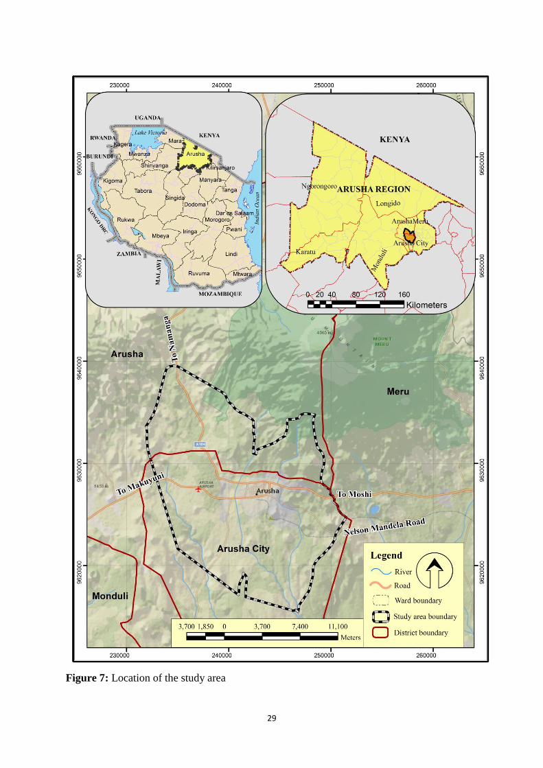
29
Figure 7: Location of the study area
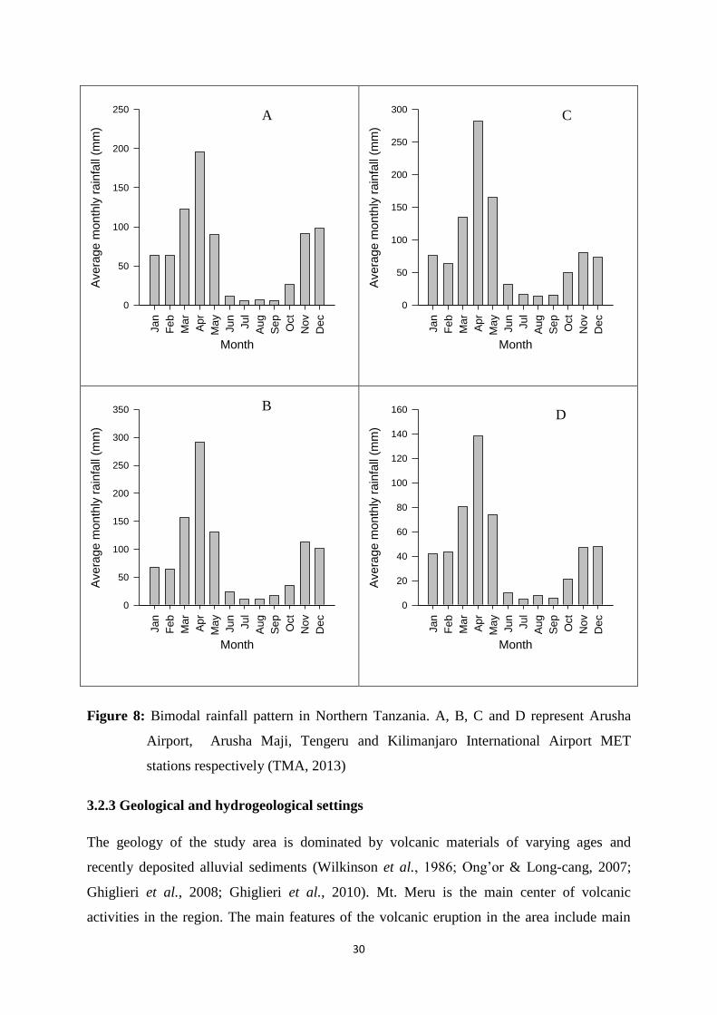
30
Month
Ja
n
Feb
Mar
Apr
May
Ju
n
Ju
l
Aug
Sep
Oct
Nov
Dec
Avera
ge m
onth
ly r
ain
fall
(mm
)
0
50
100
150
200
250
Month
Ja
n
Feb
Mar
Apr
May
Ju
n
Ju
l
Aug
Sep
Oct
Nov
Dec
Avera
ge m
onth
ly r
ain
fall
(mm
)
0
50
100
150
200
250
300
Month
Ja
n
Feb
Mar
Apr
May
Ju
n
Ju
l
Aug
Sep
Oct
Nov
Dec
Avera
ge m
onth
ly r
ain
fall
(mm
)
0
50
100
150
200
250
300
350
Month
Ja
n
Feb
Mar
Apr
May
Ju
n
Ju
l
Aug
Sep
Oct
Nov
Dec
Avera
ge m
onth
ly r
ain
fall
(mm
)
0
20
40
60
80
100
120
140
160
Figure 8: Bimodal rainfall pattern in Northern Tanzania. A, B, C and D represent Arusha
Airport, Arusha Maji, Tengeru and Kilimanjaro International Airport MET
stations respectively (TMA, 2013)
3.2.3 Geological and hydrogeological settings
The geology of the study area is dominated by volcanic materials of varying ages and
recently deposited alluvial sediments (Wilkinson et al., 1986; Ong‘or & Long-cang, 2007;
Ghiglieri et al., 2008; Ghiglieri et al., 2010). Mt. Meru is the main center of volcanic
activities in the region. The main features of the volcanic eruption in the area include main
A C
B D

31
cone deposits, mantling ash, lahars, lava flows, pyroclastic materials, tuffs, pumice,
agglomerates and volcanic rocks such basalts (Nanyaro et al., 1984; Ong‘or & Long-cang,
2007). Some of these volcanic features have been depicted in hydrogeologic map (Fig. 9)
together with the cross section derived from hydrogeological map running from the steep
slopes of Mt. Meru towards the foot of the Mountain (Fig. 10). Volcanic rocks are mainly
lava flows (basaltic to phonolitic and nephelinitic tuff). These materials, if not fractured or
weathered they act as aquitard which favor groundwater movement down the slope (Flint et
al., 2001; Wilson & Guan, 2004). The properties of these geological formations normally
change with time due to various physical chemical reactions such as weathering and
subsequent volcanic and tectonic activities. Mount Meru region is dominated by volcanic and
sedimentary hydrogeologic formations with various mineralogy compositions. These include
fluorapatite, natrite, halite, sylvite, aphthitalite, calcite, goethite, phillipsite, chabazite,
augite, sanidine, analcime, leucite, nepheline, anorthoclase, biotite, cancrinite, riebeckite,
albite and illite (Ghiglieri et al., 2012)
The area is also affected by tectonism leading to the development of fractures and faults
which act as conduit to groundwater flows in some areas (Ghiglieri et al., 2010). Figure 9
shows the fault system within the main cone deposits of pyroclastic materials with
subordinate nephelinitic and phonolitic lavas. The fault lines are assumed to be avenue of
huge groundwater flows that manifest through numerous springs which discharge into Themi
River. Volcanic sediments and alluvium derived from different volcanic materials such as
ashes, pyroclastic materials, weathered and fractured volcanic formation (e.g., basalts),
phonolitic to nephelinitic formation form the major potential aquifers in the study area
(Ghiglieri et al., 2010). However, mantling ash, volcanic ash and tuff, and sedimentary
formations particularly fine grained alluvial sediments are characterized by low
transmissivity which become practically impermeable. In most cases such hydrogeological
units act as aquitard or low yield aquifers. Groundwater recharge is mainly taking place in
high elevation on the slopes of Mt. Meru along fractured formations as well as through
infiltration in valleys or depression zones with medium to coarse grain sizes (Ghiglieri et al.,
2010). Groundwater potentiality in fractured formation is also supported by a number of
springs around the fault zone (Fig. 9), northeastern side of the study area. Springs‘ flows from
this zone are very high particularly after or at the end of long rains. For example in May 2015
a total of 25 698 m3/d was abstracted from the springs by AUWSA for public water supply.
This amount is only the portion of groundwater discharged from springs along this fault, the

32
remaining water flows into Themi River which is one among the perennial and reliable water
sources in the study area. Overall, most rivers and streams originate from springs located on
the slopes of Mt. Meru particularly in fractured formations at high elevations. Major rivers
include Themi, Kijenge, Ngarenaro, Burka and Engare Olmotonyi (Fig. 9)
Based on the hydraulic head observed from existing production wells groundwater flows
from north to south direction towards the foot of Mt. Meru. This is well supported by wells
W12 and W17 with hydraulic heads at 1356 and 1348 m a.s.l. respectively. Thus groundwater
flows from W12 with high hydraulic head also located at elevated area to W17 with hydraulic
head difference of 8 m at a distance of 1.2 km. Figure 11 shows potential aquifers as derived
from well logs data in the study area (Appendix 3). The W12, W15, W16 and W9 are among
the existing production wells in the area. W19 taps water from weathered or fractured basalt
aquifer whereas, the rest collect water from either formation depending on the arrangement of
hydrogeological units and position of the screens. This indicates that groundwater occurs
both in fractured formation and volcanic sediment hosted aquifers. As mentioned before,
fractured formations seem to be more productive aquifers as well as potential recharge zones
in the area. Though volcanic sediment hosted aquifers cannot be ignored as they also produce
substantial amount of water in the area. A good example of the well tapping water from
volcanic sediment formation is W12 which discharge up to 192 m3/h. However, more
information are needed to delineate the aquifer geometry as most wells used in this study lack
hydrogeological data including well logs, depth and specific yield.
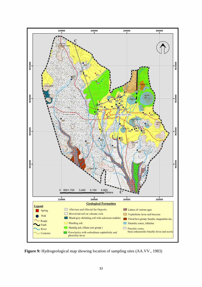
33
Figure 9: Hydrogeological map showing location of sampling sites (AA.VV., 1983)
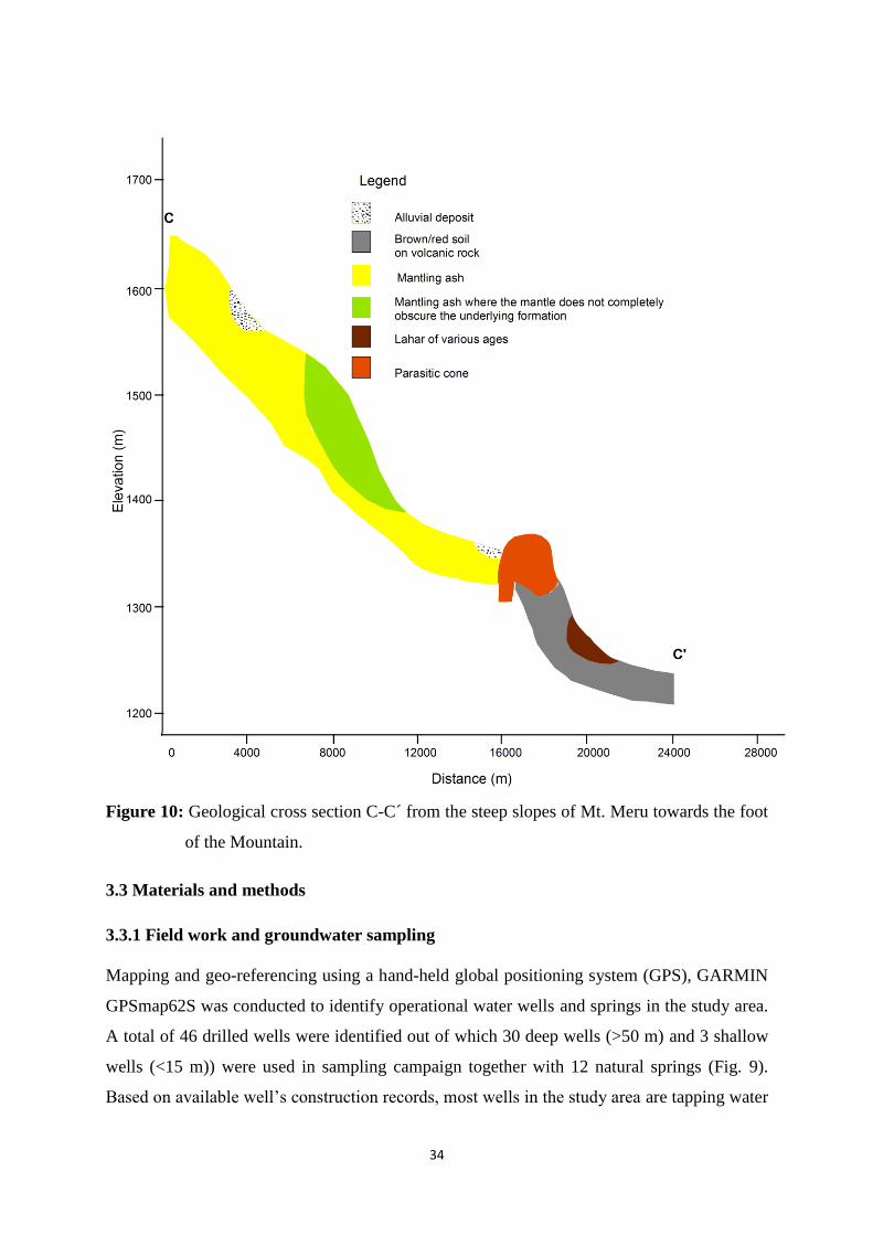
34
Figure 10: Geological cross section C-C´ from the steep slopes of Mt. Meru towards the foot
of the Mountain.
3.3 Materials and methods
3.3.1 Field work and groundwater sampling
Mapping and geo-referencing using a hand-held global positioning system (GPS), GARMIN
GPSmap62S was conducted to identify operational water wells and springs in the study area.
A total of 46 drilled wells were identified out of which 30 deep wells (>50 m) and 3 shallow
wells (<15 m)) were used in sampling campaign together with 12 natural springs (Fig. 9).
Based on available well‘s construction records, most wells in the study area are tapping water
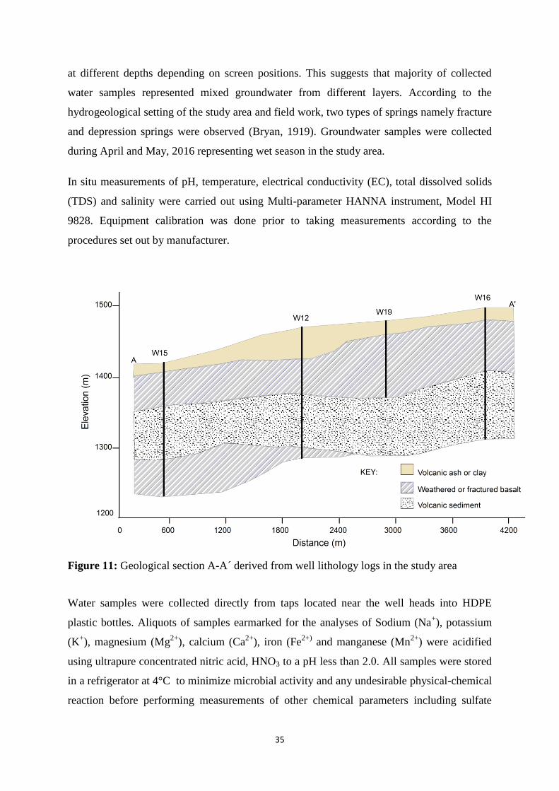
35
at different depths depending on screen positions. This suggests that majority of collected
water samples represented mixed groundwater from different layers. According to the
hydrogeological setting of the study area and field work, two types of springs namely fracture
and depression springs were observed (Bryan, 1919). Groundwater samples were collected
during April and May, 2016 representing wet season in the study area.
In situ measurements of pH, temperature, electrical conductivity (EC), total dissolved solids
(TDS) and salinity were carried out using Multi-parameter HANNA instrument, Model HI
9828. Equipment calibration was done prior to taking measurements according to the
procedures set out by manufacturer.
Figure 11: Geological section A-A´ derived from well lithology logs in the study area
Water samples were collected directly from taps located near the well heads into HDPE
plastic bottles. Aliquots of samples earmarked for the analyses of Sodium (Na+), potassium
(K+), magnesium (Mg
2+), calcium (Ca
2+), iron (Fe
2+) and manganese (Mn
2+) were acidified
using ultrapure concentrated nitric acid, HNO3 to a pH less than 2.0. All samples were stored
in a refrigerator at 4°C to minimize microbial activity and any undesirable physical-chemical
reaction before performing measurements of other chemical parameters including sulfate
36
(SO42-
), chloride (Cl-), nitrate (NO3
-), bicarbonate (HCO3
-), fluoride (F
-) and phosphate
(PO43-
) (Sundaram et al., 2009; APHA, 2012).
3.3.2 Laboratory analyses
All groundwater samples were analyzed for major cations and anions using various methods.
Bicarbonate (HCO3-) was determined by titration method using standard sulfuric acid and
bromcresol green indicator for end point detection. The determination of SO42-
(SulfaVer 4
method), NO3- (Cadmium reduction method), and PO4
3- (PhosVer 3, Ascobic acid method)
were carried out using HACH DR 2800 spectrophotometer by powder pillow test. Chloride
concentration was determined by Argentometric titration method using standard silver nitrate
(AgNO3) titrant and potassium chromate indicator solution (APHA, 2012). Fluoride content
was determined by ion selective electrode method. The fluoride concentration was read
directly from the meter calibrated with standard fluoride solution before use. Fluoride buffer
was prepared from glacial acetic acid, sodium chloride and 1, 2-
cyclohexylenediaminetetraacetic acid.
All major cations (Na+, K
+, Mg
2+, Ca
2+) and trace elements (Fe
2+ and Mn
2+) analyses were
carried out at the Ardhi University Laboratory in Dar es Salaam by Atomic absorption
Spectrometer (AAS) PerkinElmer Analyst 100. Samples were filtered (0.45 µm) before
introduced into the flame for conversion from aerosols into atomic vapour which absorbs
light from the primary source. The concentration of individual element was determined by
measuring the amount of light absorbed relative to the standard solution under a specific
wavelength. The accuracy of the major ions analyses was checked by calculating the charge
balance error.
3.3.3 Geostatistical analysis
Cluster analysis, multivariate statistical analysis technique, was carried out using
Paleontological Statistics (PAST) Software Package, Version 3.08 (Hammer et al., 2001).
The technique was employed to understand the relationship between variables from different
sampling sites and their relevance with respect to groundwater quality in the study area. The
clusters were established based on similarities of variables under consideration (Davidson &
Ravi, 2005; Mooi & Sarstedt, 2010). One way ANOVA, single factor was used to compare
means of various parameters between spring and well waters. It was also applied for
comparing means of different water groups generated by cluster analysis. The correlation

37
analysis was carried out for hydrogeochemical characteristics of analyzed water samples and
the significance of correlation coefficients were tested using the statistical software, SPSS
version 21. A geographical Information System (GIS) Software Package, ArcGIS version
10.1 was used to generate various maps in this study. Geostatistical analysis tool was
employed in establishing groundwater quality spatial variation.
3.3.4 Piper diagram
Piper diagram was used to graphically represent chemistry of groundwater samples in the
study area (Piper, 1944; Sadashivaiah et al., 2008; Srinivas et al., 2014). It comprises of three
plots; a ternary diagram in the lower left representing the cations, another ternary diagram in
the lower right representing the anions and a diamond plot in the middle representing a
combination of the two ternary diagrams. The piper diagram was created using GW_Chart
v.1.29.0 and it was employed to understand and identify different water composition or type
through chemical relationships among groundwater samples (Utom et al., 2013).
3.4 Results
3.4.1 Variation in physical-chemical properties
The results of groundwater physical chemical characteristics in the study area are presented
in Table 4. The temperature for the spring water ranged from 16.7 to 22.9 °C and averaged
19.9 ±1.9 °C, while that of well water ranged from 19.4 to 24.5 °C and averaged 21.9 ±1.1
°C. The lowest temperature in spring water was recorded at high altitude about 1600 m above
sea level (a.s.l.) and the highest temperature at an elevation of 1322 m a.s.l. A slight
temperature variations observed in both spring and well waters are generally influenced by
different ambient conditions from low to high elevations than aquifer type. The average value
of pH in spring and well waters were 7.2 ± 0.7 and 7.5 ± 0.5 respectively. In spring water the
pH varied from 6.42 to 8.26, while in well water it ranged from 6.47 to 8.9. About 42% and
15% of spring and well waters showed slightly acidic conditions (pH values less than 7.0),
respectively.
Electrical conductivity (EC) in well water varied from 286 to 1634 µS/cm with an average
value of 638 ± 330 µS/cm which is relatively high to WHO recommended limit (500 µS/cm).
Low EC values were detected in spring waters which ranged from 157 to 781 µS/cm with an
average value 399 ± 225 µS/cm.

38
Table 4: Groundwater chemistry in the study area
SN Location SID pH Temp EC TDS Sal. SO42- NO3
- F- Cl- HCO3- PO4
3- Na+ K+ Mg2+ Ca2+ Fe2+ Mn2+
1 Lemara spring S01 6.56 22.9 781 422 0.4 43 2.9 1.78 59.02 264 0.49 92.20 21.93 15.04 49.64 0.09 0.05
2 Ilboru Spring S02 7.03 20.3 311 166 0.2 10 4.2 1.35 5.04 243 0.31 42.58 15.46 12.09 19.39 1.93 0.01
3 Kiranyi Spring S03 7.92 20.4 467 251 0.2 13 6.0 3.66 12.23 195 0.55 84.34 24.32 12.66 15.36 0.11 <0.01
4 Engarendolu S04 6.56 21.5 671 362 0.4 19 17.3 1.88 32.44 280 0.55 85.06 37.35 14.40 35.38 0.03 <0.01
5 LSB Spring S05 6.42 19.6 398 214 0.2 20 10.9 1.18 5.32 290 0.30 76.73 17.62 13.69 37.51 0.07 0.01
6 Masama Chini S06 8.26 16.8 165 88 0.1 0 1.6 3.28 2.66 170 0.34 41.33 6.58 3.70 6.13 0.88 <0.01
7 Masama Kati S07 7.83 16.7 162 86 0.1 1 1.9 3.01 3.19 160 0.45 44.72 7.24 3.45 4.58 0.07 0.01
8 Masama Juu S08 8.10 18.1 158 84 0.1 1 1.7 2.71 2.66 160 0.41 46.57 7.82 3.25 4.41 0.06 0.01
9 Machare Spring S09 6.42 21.6 350 187 0.2 12 7.8 0.81 15.95 268 1.02 79.18 7.12 13.96 31.64 0.05 <0.01
10 Baraa Spring S10 6.76 20.3 209 111 0.1 0 2.1 1.45 2.66 216 0.42 51.45 7.05 9.70 14.31 0.08 0.01
11 Selian Spring S11 7.03 20.5 744 403 0.4 22 2.5 5.45 13.19 180 0.35 152.96 14.73 10.85 25.14 0.05 <0.01
12 Njoro Spring S12 7.67 19.9 376 202 0.2 2 2.4 5.36 2.13 190 0.49 57.77 20.72 2.67 8.73 0.06 <0.01
13 Sombetini Sec W01 7.18 22.6 601 323 0.3 11 8.8 3.50 26.31 188 1.02 84.62 28.09 9.51 17.51 0.10 0.07
14 Sokoni I W02 8.90 24.3 1114 606 0.6 14 0.7 3.87 98.10 228 0.58 141.79 26.02 5.54 10.67 0.06 <0.01
15 Sokoni I P/S W03 7.28 24.5 833 450 0.4 20 1.0 4.53 69.14 256 1.29 115.84 25.41 11.98 25.90 0.06 0.33
16 Emco W04 7.73 21.6 450 241 0.2 5 0.5 3.27 18.64 264 0.19 76.98 20.17 11.66 18.00 0.08 0.02
17 Lemara P/S W05 6.59 22.7 640 344 0.3 26 5.3 1.75 60.41 270 0.50 89.72 27.72 14.10 50.28 0.12 <0.01
18 Omahe W06 7.49 21.0 1216 667 0.7 40 0.7 2.61 143.29 354 0.42 189.50 56.03 13.56 45.56 0.04 <0.01
19 Old Sanawari W07 7.36 21.4 305 163 0.2 3 0.6 2.28 4.25 210 0.68 46.45 12.22 9.86 12.77 0.08 <0.01
20 Ilkiloriti W08 7.50 21.3 362 193 0.2 6 2.0 5.84 5.32 238 1.48 103.17 8.87 5.24 4.86 0.32 0.01
21 Moivo II W09 7.89 21.1 369 198 0.2 12 1.3 1.99 5.85 208 0.84 54.22 12.47 9.12 8.40 0.13 0.01
22 Sanawari primary W10 7.94 21.4 380 203 0.2 4 0.8 3.12 7.44 223 0.85 54.52 13.22 7.75 9.68 0.54 <0.01
23 Lorovani Bondeni W11 7.71 20.5 328 176 0.2 5 0.9 4.88 3.19 205 1.22 51.15 13.51 4.35 5.31 0.07 0.01
24 Oltulelei W12 7.12 19.4 382 205 0.2 6 2.6 4.22 6.91 211 1.00 73.88 16.54 7.79 9.96 0.04 0.01
25 Ilkiurei W13 7.84 22.0 494 265 0.3 7 4.2 6.03 22.76 215 0.98 88.88 15.23 4.70 8.14 0.06 <0.01
26 Loruvan Yard W14 7.65 21.1 336 180 0.2 4 1.8 3.73 4.79 245 1.00 117.44 15.71 8.51 9.86 0.07 0.01
27 Kiranyi Mission W15 7.37 21.7 468 251 0.2 11 1.3 4.47 15.04 254 0.83 93.87 18.02 8.46 12.68 0.07 <0.01
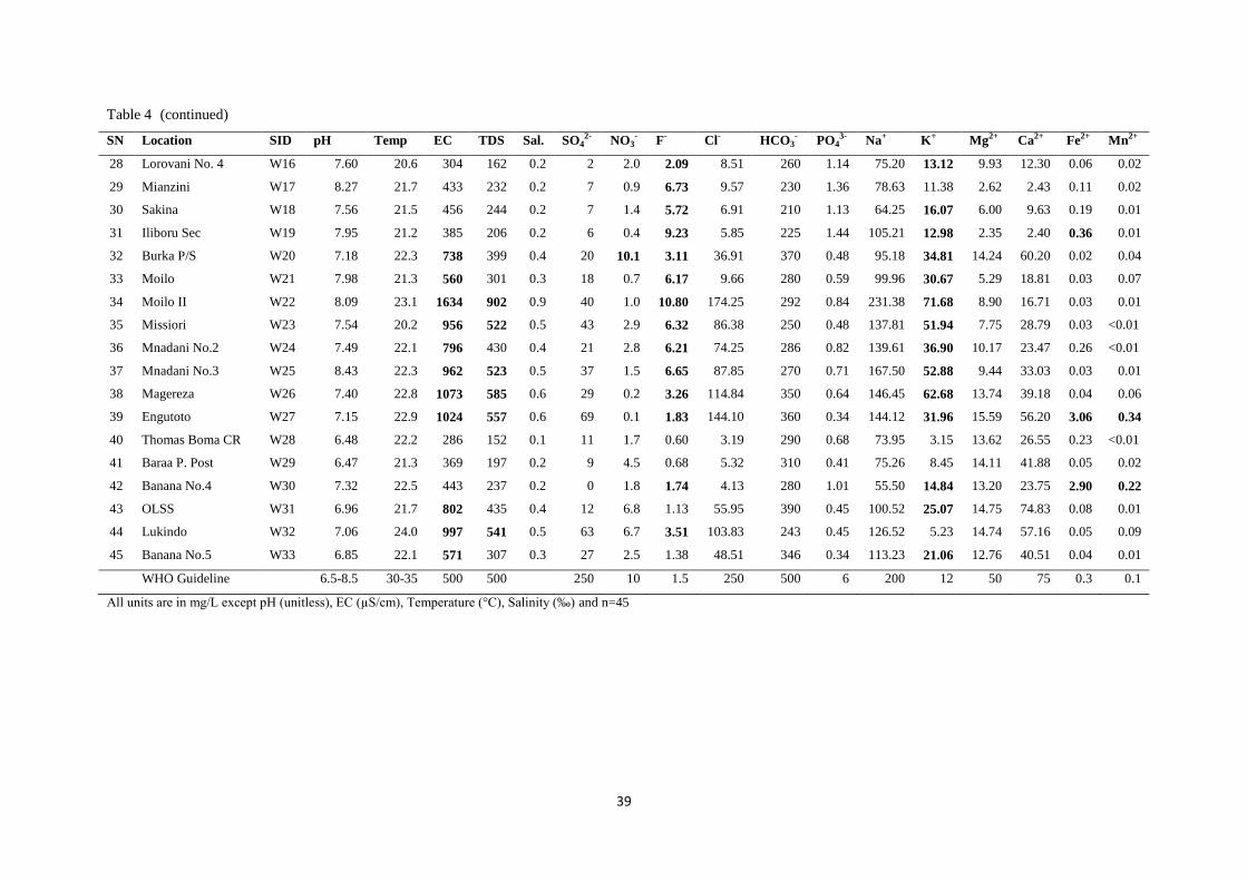
39
Table 4 (continued)
SN Location SID pH Temp EC TDS Sal. SO42- NO3
- F- Cl- HCO3- PO4
3- Na+ K+ Mg2+ Ca2+ Fe2+ Mn2+
28 Lorovani No. 4 W16 7.60 20.6 304 162 0.2 2 2.0 2.09 8.51 260 1.14 75.20 13.12 9.93 12.30 0.06 0.02
29 Mianzini W17 8.27 21.7 433 232 0.2 7 0.9 6.73 9.57 230 1.36 78.63 11.38 2.62 2.43 0.11 0.02
30 Sakina W18 7.56 21.5 456 244 0.2 7 1.4 5.72 6.91 210 1.13 64.25 16.07 6.00 9.63 0.19 0.01
31 Iliboru Sec W19 7.95 21.2 385 206 0.2 6 0.4 9.23 5.85 225 1.44 105.21 12.98 2.35 2.40 0.36 0.01
32 Burka P/S W20 7.18 22.3 738 399 0.4 20 10.1 3.11 36.91 370 0.48 95.18 34.81 14.24 60.20 0.02 0.04
33 Moilo W21 7.98 21.3 560 301 0.3 18 0.7 6.17 9.66 280 0.59 99.96 30.67 5.29 18.81 0.03 0.07
34 Moilo II W22 8.09 23.1 1634 902 0.9 40 1.0 10.80 174.25 292 0.84 231.38 71.68 8.90 16.71 0.03 0.01
35 Missiori W23 7.54 20.2 956 522 0.5 43 2.9 6.32 86.38 250 0.48 137.81 51.94 7.75 28.79 0.03 <0.01
36 Mnadani No.2 W24 7.49 22.1 796 430 0.4 21 2.8 6.21 74.25 286 0.82 139.61 36.90 10.17 23.47 0.26 <0.01
37 Mnadani No.3 W25 8.43 22.3 962 523 0.5 37 1.5 6.65 87.85 270 0.71 167.50 52.88 9.44 33.03 0.03 0.01
38 Magereza W26 7.40 22.8 1073 585 0.6 29 0.2 3.26 114.84 350 0.64 146.45 62.68 13.74 39.18 0.04 0.06
39 Engutoto W27 7.15 22.9 1024 557 0.6 69 0.1 1.83 144.10 360 0.34 144.12 31.96 15.59 56.20 3.06 0.34
40 Thomas Boma CR W28 6.48 22.2 286 152 0.1 11 1.7 0.60 3.19 290 0.68 73.95 3.15 13.62 26.55 0.23 <0.01
41 Baraa P. Post W29 6.47 21.3 369 197 0.2 9 4.5 0.68 5.32 310 0.41 75.26 8.45 14.11 41.88 0.05 0.02
42 Banana No.4 W30 7.32 22.5 443 237 0.2 0 1.8 1.74 4.13 280 1.01 55.50 14.84 13.20 23.75 2.90 0.22
43 OLSS W31 6.96 21.7 802 435 0.4 12 6.8 1.13 55.95 390 0.45 100.52 25.07 14.75 74.83 0.08 0.01
44 Lukindo W32 7.06 24.0 997 541 0.5 63 6.7 3.51 103.83 243 0.45 126.52 5.23 14.74 57.16 0.05 0.09
45 Banana No.5 W33 6.85 22.1 571 307 0.3 27 2.5 1.38 48.51 346 0.34 113.23 21.06 12.76 40.51 0.04 0.01
WHO Guideline 6.5-8.5 30-35 500 500 250 10 1.5 250 500 6 200 12 50 75 0.3 0.1
All units are in mg/L except pH (unitless), EC (µ /cm), Temperature (°C), alinity (‰) and n=45
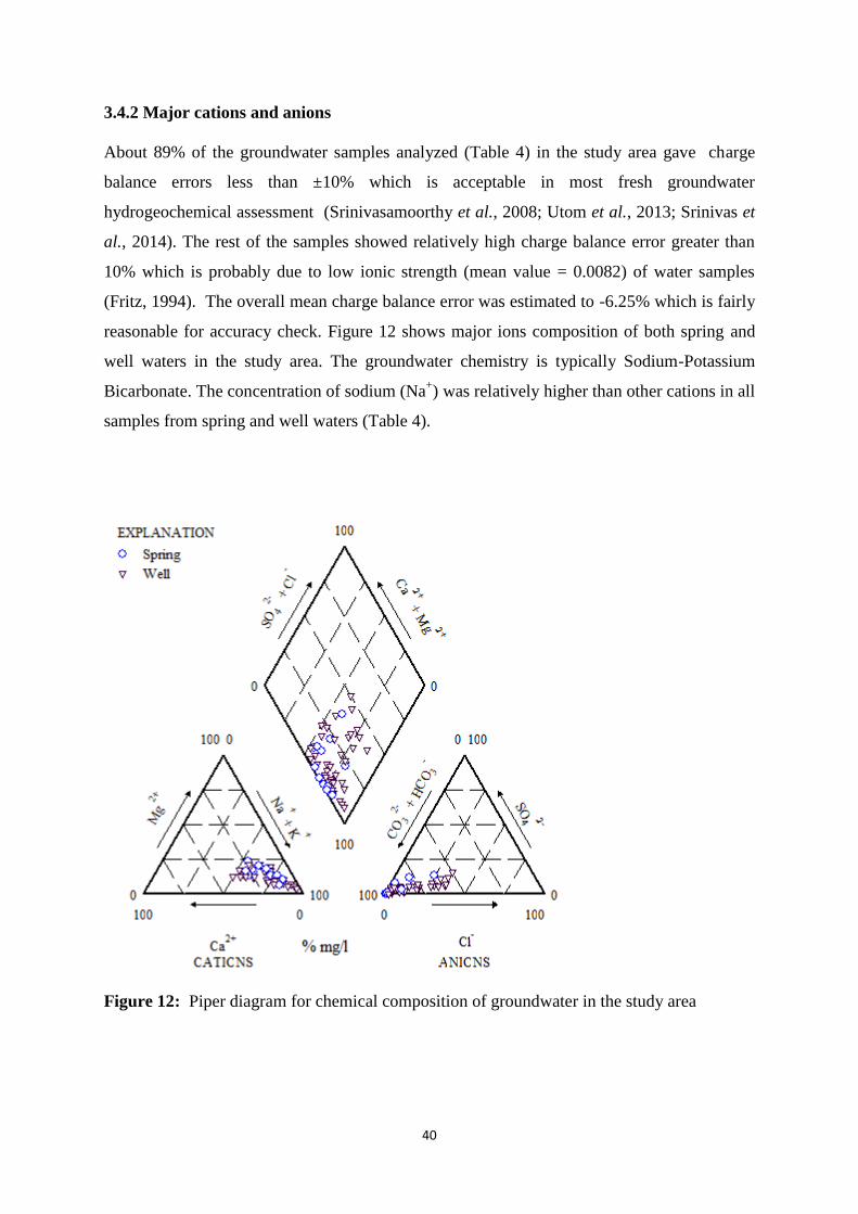
40
3.4.2 Major cations and anions
About 89% of the groundwater samples analyzed (Table 4) in the study area gave charge
balance errors less than ±10% which is acceptable in most fresh groundwater
hydrogeochemical assessment (Srinivasamoorthy et al., 2008; Utom et al., 2013; Srinivas et
al., 2014). The rest of the samples showed relatively high charge balance error greater than
10% which is probably due to low ionic strength (mean value = 0.0082) of water samples
(Fritz, 1994). The overall mean charge balance error was estimated to -6.25% which is fairly
reasonable for accuracy check. Figure 12 shows major ions composition of both spring and
well waters in the study area. The groundwater chemistry is typically Sodium-Potassium
Bicarbonate. The concentration of sodium (Na+) was relatively higher than other cations in all
samples from spring and well waters (Table 4).
Figure 12: Piper diagram for chemical composition of groundwater in the study area
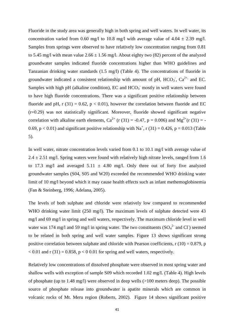
41
Fluoride in the study area was generally high in both spring and well waters. In well water, its
concentration varied from 0.60 mg/l to 10.8 mg/l with average value of 4.04 ± 2.39 mg/l.
Samples from springs were observed to have relatively low concentration ranging from 0.81
to 5.45 mg/l with mean value 2.66 ± 1.56 mg/l. About eighty two (82) percent of the analyzed
groundwater samples indicated fluoride concentrations higher than WHO guidelines and
Tanzanian drinking water standards (1.5 mg/l) (Table 4). The concentrations of fluoride in
groundwater indicated a consistent relationship with amount of pH, HCO3-, Ca
2+, and EC.
Samples with high pH (alkaline condition), EC and HCO3- mostly in well waters were found
to have high fluoride concentrations. There was a significant positive relationship between
fluoride and pH, r (31) = 0.62, p < 0.01), however the correlation between fluoride and EC
(r=0.29) was not statistically significant. Moreover, fluoride showed significant negative
correlation with alkaline earth elements, Ca2+
(r (31) = -0.47, p = 0.006) and Mg2+
(r (31) = -
0.69, p < 0.01) and significant positive relationship with Na+, r (31) = 0.426, p = 0.013 (Table
5).
In well water, nitrate concentration levels varied from 0.1 to 10.1 mg/l with average value of
2.4 ± 2.51 mg/l. Spring waters were found with relatively high nitrate levels, ranged from 1.6
to 17.3 mg/l and averaged 5.11 ± 4.80 mg/l. Only three out of forty five analyzed
groundwater samples (S04, S05 and W20) exceeded the recommended WHO drinking water
limit of 10 mg/l beyond which it may cause health effects such as infant methemoglobinemia
(Fan & Steinberg, 1996; Adelana, 2005).
The levels of both sulphate and chloride were relatively low compared to recommended
WHO drinking water limit (250 mg/l). The maximum levels of sulphate detected were 43
mg/l and 69 mg/l in spring and well waters, respectively. The maximum chloride level in well
water was 174 mg/l and 59 mg/l in spring water. The two constituents (SO42-
and Cl-) seemed
to be related in both spring and well water samples. Figure 13 shows significant strong
positive correlation between sulphate and chloride with Pearson coefficients, r (10) = 0.879, p
< 0.01 and r (31) = 0.858, p < 0 0.01 for spring and well waters, respectively.
Relatively low concentrations of dissolved phosphate were observed in most spring water and
shallow wells with exception of sample S09 which recorded 1.02 mg/L (Table 4). High levels
of phosphate (up to 1.48 mg/l) were observed in deep wells (>100 meters deep). The possible
source of phosphate release into groundwater is apatite minerals which are common in
volcanic rocks of Mt. Meru region (Roberts, 2002). Figure 14 shows significant positive
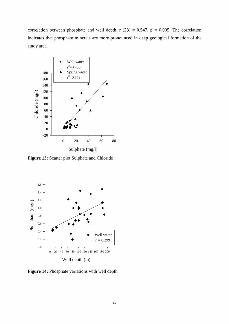
42
correlation between phosphate and well depth, r (23) = 0.547, p = 0.005. The correlation
indicates that phosphate minerals are more pronounced in deep geological formation of the
study area.
Sulphate (mg/l)
0 20 40 60 80
Chlo
ride
(mg/l
)
-20
0
20
40
60
80
100
120
140
160
180
Well water
r2=0.736
Spring water
r2=0.773
Figure 13: Scatter plot Sulphate and Chloride
Well depth (m)
0 20 40 60 80 100 120 140 160 180 200
Ph
osp
hat
e (m
g/l
)
0.0
0.2
0.4
0.6
0.8
1.0
1.2
1.4
1.6
Well water
r2 = 0.299
Figure 14: Phosphate variations with well depth

43
3.4.3 Trace elements (Fe and Mn)
Iron concentration varied from 0.02 to 3.06 mg/l (well water) and 0.03 to 1.93 mg/l (spring
water). More than 84% of the analyzed water samples had Fe contents less than
recommended maximum WHO limit (0.3 mg/l). Furthermore the concentration of Manganese
was generally very low. About 36% of analyzed water samples were below the detection
limits (0.01 mg/l). However, only two samples (W03 and W27) out of forty five were
observed to have manganese levels beyond the recommended WHO guideline (0.1 mg/l).
Generally, the levels of iron and manganese detected in this study were relatively low which
have no significant health effect or engineering problems in water supply infrastructures.
3.4.4 Multivariate analysis
Analyzed water samples were grouped into four main categories, the first group comprises of
cluster A and B with a total of fourteen samples which indicated great than 60% similarity.
Six out of fourteen in this group being samples from spring water. Cluster C has a total of six
(6) sampling sites all being wells. The third group (Cluster D) has twelve (12) sampling sites
with great than 60% similarity and one of its sub-clusters has greater than 90% similarity
index. The last group (Cluster E) comprises of four (4) sampling sites (springs) with great
than 95% similarity. However, out of 45 sampling sites, five showed less than 50% similarity
with other clusters (Fig. 15).
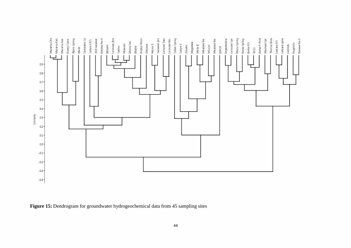
44
Figure 15: Dendrogram for groundwater hydrogeochemical data from 45 sampling sites
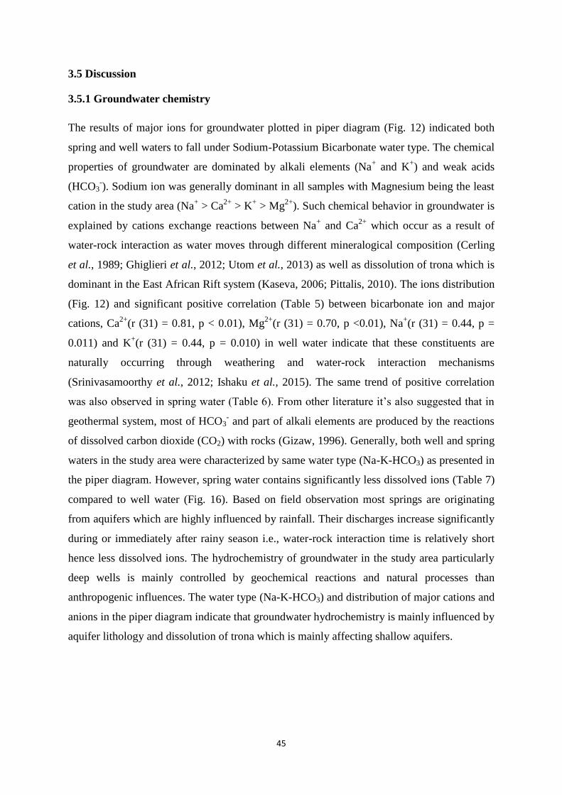
45
3.5 Discussion
3.5.1 Groundwater chemistry
The results of major ions for groundwater plotted in piper diagram (Fig. 12) indicated both
spring and well waters to fall under Sodium-Potassium Bicarbonate water type. The chemical
properties of groundwater are dominated by alkali elements (Na+ and K
+) and weak acids
(HCO3-). Sodium ion was generally dominant in all samples with Magnesium being the least
cation in the study area (Na+ > Ca
2+ > K
+ > Mg
2+). Such chemical behavior in groundwater is
explained by cations exchange reactions between Na+ and Ca
2+ which occur as a result of
water-rock interaction as water moves through different mineralogical composition (Cerling
et al., 1989; Ghiglieri et al., 2012; Utom et al., 2013) as well as dissolution of trona which is
dominant in the East African Rift system (Kaseva, 2006; Pittalis, 2010). The ions distribution
(Fig. 12) and significant positive correlation (Table 5) between bicarbonate ion and major
cations, Ca2+
(r (31) = 0.81, p < 0.01), Mg2+
(r (31) = 0.70, p <0.01), Na+(r (31) = 0.44, p =
0.011) and K+(r (31) = 0.44, p = 0.010) in well water indicate that these constituents are
naturally occurring through weathering and water-rock interaction mechanisms
(Srinivasamoorthy et al., 2012; Ishaku et al., 2015). The same trend of positive correlation
was also observed in spring water (Table 6). From other literature it‘s also suggested that in
geothermal system, most of HCO3- and part of alkali elements are produced by the reactions
of dissolved carbon dioxide (CO2) with rocks (Gizaw, 1996). Generally, both well and spring
waters in the study area were characterized by same water type (Na-K-HCO3) as presented in
the piper diagram. However, spring water contains significantly less dissolved ions (Table 7)
compared to well water (Fig. 16). Based on field observation most springs are originating
from aquifers which are highly influenced by rainfall. Their discharges increase significantly
during or immediately after rainy season i.e., water-rock interaction time is relatively short
hence less dissolved ions. The hydrochemistry of groundwater in the study area particularly
deep wells is mainly controlled by geochemical reactions and natural processes than
anthropogenic influences. The water type (Na-K-HCO3) and distribution of major cations and
anions in the piper diagram indicate that groundwater hydrochemistry is mainly influenced by
aquifer lithology and dissolution of trona which is mainly affecting shallow aquifers.
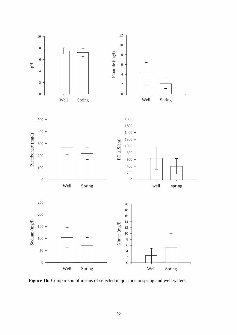
46
Well Spring
pH
0
2
4
6
8
10
Well Spring
Flu
ori
de
(mg/l
)
0
2
4
6
8
10
12
Well Spring
Bic
arb
on
ate
(mg
/l)
0
100
200
300
400
500
well spring
EC
(µ
S/c
m)
0
200
400
600
800
1000
1200
1400
1600
1800
Well Spring
Sodiu
m (
mg/l
)
0
50
100
150
200
250
Well Spring
Nit
rate
(m
g/l
)
0
2
4
6
8
10
12
14
16
18
20
Figure 16: Comparison of means of selected major ions in spring and well waters
47
Table 5: Pearson correlation matrix for samples from well water
pH Temp EC TDS Sal. SO42- NO3
- F- Cl- HCO3- PO4
3- Na+ K+ Mg2+ Ca2+
pH 1
Temp 0.04 1
EC 0.21 0.53 1
TDS 0.21 0.53 1.00 1
Sal. 0.24 0.47 0.99 0.99 1
SO42- -0.10 0.40 0.76 0.76 0.75 1
NO3- -0.45 0.14 0.03 0.03 -0.01 0.08 1
F- 0.62 -0.02 0.29 0.30 0.29 0.07 -0.24 1
Cl- 0.11 0.51 0.97 0.97 0.97 0.84 -0.04 0.18 1
HCO3- -0.38 0.19 0.45 0.45 0.45 0.44 0.17 -0.34 0.49 1
PO43- 0.30 -0.17 -0.39 -0.39 -0.38 -0.51 -0.21 0.48 -0.43 -0.60 1
Na+ 0.24 0.37 0.90 0.90 0.90 0.70 -0.10 0.43 0.89 0.44 -0.26 1
K+ 0.23 0.18 0.83 0.83 0.84 0.54 -0.07 0.36 0.78 0.44 -0.31 0.81 1
Mg2+ -0.69 0.35 0.30 0.30 0.28 0.45 0.36 -0.69 0.39 0.70 -0.67 0.17 0.19 1
Ca2+ -0.55 0.33 0.46 0.45 0.43 0.61 0.52 -0.47 0.50 0.81 -0.70 0.31 0.30 0.84 1
Green color indicates negative correlation (r < -0.5) and pink color, positive correlation (r > 0.5)
As to a large extent the hydrogeological formation of the region is characterized by the
presence of sodium and potassium rich minerals such as nepheline, chabazite, sanidine,
cancrinite, phillipsite and anorthoclase to mention few (Ghiglieri et al., 2012). Generally,
sodium and potassium ions were relatively high in all groundwater samples (Table 4)
indicating the influence of water-rock interaction in determining groundwater chemistry of
the study area. This is also supported by low levels of anthropogenic indicators such as
nitrate, chloride and sulphate observed in deep wells (Table 4).
Moreover, statistical error bars of selected major ions were plotted to compare water clusters
(Fig. 17). A slight difference between clusters was observed from the error bar plots.
Additionally, the results of statistical test using one way ANOVA, single factor indicated a
significance difference between clusters for the selected major ions (Table 8). The differences
shown between clusters are probably due to heterogeneity of the volcanic aquifers in the
study area (Ong‘or & Long-cang, 2007). However, the groundwater hydrochemistry of the
study area remain the same with Na-K-HCO3 water type.
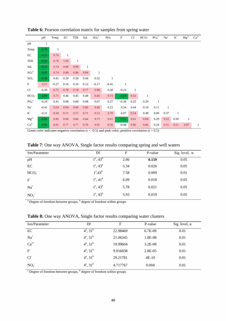
48
Table 6: Pearson correlation matrix for samples from spring water
pH Temp EC TDS Sal. SO42- NO3
- F- Cl- HCO3- PO4
3- Na+ K+ Mg2+ Ca2+
pH 1
Temp -0.76 1
EC -0.53 0.76 1
TDS -0.53 0.76 1.00 1
Sal. -0.55 0.74 0.98 0.98 1
SO42- -0.61 0.74 0.88 0.88 0.84 1
NO3- -0.56 0.41 0.39 0.39 0.44 0.32 1
F- 0.57 -0.27 0.16 0.16 0.12 -0.17 -0.41 1
Cl- -0.50 0.72 0.78 0.78 0.77 0.88 0.30 -0.23 1
HCO3- -0.88 0.71 0.46 0.45 0.48 0.60 0.74 -0.69 0.52 1
PO43- -0.29 0.41 0.08 0.08 0.08 0.07 0.27 -0.26 0.25 0.29 1
Na+ -0.41 0.54 0.84 0.84 0.80 0.66 0.22 0.34 0.44 0.19 0.11 1
K+ -0.31 0.56 0.71 0.71 0.71 0.53 0.70 0.07 0.54 0.48 0.00 0.37 1
Mg2+ -0.81 0.82 0.66 0.66 0.64 0.75 0.61 -0.52 0.61 0.84 0.29 0.52 0.50 1
Ca2+ -0.85 0.81 0.77 0.77 0.76 0.91 0.56 -0.44 0.80 0.86 0.24 0.55 0.51 0.87 1
Green color indicates negative correlation (r < -0.5) and pink color, positive correlation (r > 0.5)
Table 7: One way ANOVA, Single factor results comparing spring and well waters
Ion/Parameter Df F P-value ig. level, α
pH 1a, 43
b 2.06 0.159 0.05
EC 1a, 43
b 5.34 0.026 0.05
HCO3- 1
a,43
b 7.58 0.009 0.01
F- 1
a, 41
b 6.09 0.018 0.05
Na+ 1
a, 43
b 5.78 0.021 0.05
NO3- 1
a, 43
b 5.93 0.019 0.05
a Degree of freedom between groups, b degree of freedom within groups
Table 8: One way ANOVA, Single factor results comparing water clusters
Ion/Parameter Df F P-value Sig. level, α
EC 4a, 31
b 22.98469 6.7E-09 0.01
Na+ 4
a, 31
b 21.06345 1.8E-08 0.01
Ca2+
4a, 31
b 19.99604 3.2E-08 0.01
F- 4
a, 31
b 9.916838 2.8E-05 0.01
Cl- 4
a, 31
b 29.21781 4E-10 0.01
NO3- 4
a, 31
b 4.717767 0.004 0.01
a Degree of freedom between groups, b degree of freedom within groups

49
3.5.2 Fluoride
Fluoride concentration in the study area was generally high in both spring and well waters. Its
concentrations varied from one location to another indicating different mineralogy or
geological formation which may have different dissolution rate, cation exchange capacity and
precipitation in the aquifer matrix (Ghiglieri et al., 2012). Fluoride concentration indicated
positive correlation with Na+ and negative correlation with alkaline earth elements (Ca
2+ and
Mg2+
) (Table 5). This association indicates that during ionic exchange process and
precipitation when calcium ion is removed from groundwater system more Na+ and F
- ions
are being released from minerals such as fluorapatite and nepheline in the aquifer matrix.
Similar findings on fluoride behavior with alkaline earth elements (Ca2+
, Mg2+
) and alkali
metals (Na+, K
+) are well documented (Chae et al., 2007; Rafique et al., 2009; Guo et al.,
2012). Moreover, Ghiglieri et al. (2012) and Srinivasamoorthy et al., (2012) revealed that
alkaline nature of groundwater enhances fluoride releases from fluorine rich-minerals such as
fluorite (CaF2) into water system. Furthermore, according to the batch experiments conducted
(Saxena & Ahmed, 2001) at normal room temperature fluoride is easily released from parent
rocks at a pH, EC and HCO3- range of 7.6 to 8.6, 750-1750 µS/cm and 350-450 mg/l
respectively. These findings are in line with high fluoride concentrations detected in
groundwater samples with high bicarbonate and pH values. In addition, water-rock
interaction influences the concentration and rate of fluoride release into groundwater system.
Low fluoride concentration in fractured and highly permeable phonolite hosted aquifers has
been reported, and high fluoride concentration in water originating from basalt and lahars
formation (Ghiglieri et al., 2010). This suggests that variations of fluoride concentrations in
groundwater are mainly controlled by both aquifer materials and mean residence time. The
geological-hydrogeological section A-A´ (Fig. 11) constructed from well logs (Appendix 3)
indicates that most wells collect water from volcanic sediment aquifers except W19 which is
located in weathered and/or fractured basalt formation. W19 indicated high fluoride
concentration (9.23 mg/l) compared to wells W12 (4.2 mg/l) and W16 (2.09 mg/l) which tap
water from volcanic sediment aquifer.
However, it should be noted that groundwater samples were collected from different depths
within a single well depending on the position of the screens (Table 9). In the study area the
spatial distribution of fluoride concentrations indicates high fluoride concentration in
northern and northwestern parts of the study area (Appendix 1). High fluoride concentration
in this zone is probably due to dominance in basalt formation and other fluoride rich volcanic
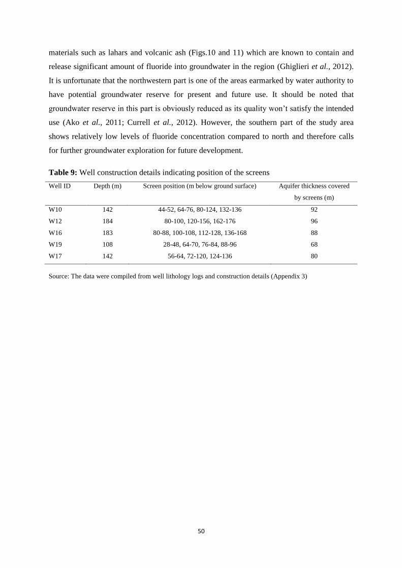
50
materials such as lahars and volcanic ash (Figs.10 and 11) which are known to contain and
release significant amount of fluoride into groundwater in the region (Ghiglieri et al., 2012).
It is unfortunate that the northwestern part is one of the areas earmarked by water authority to
have potential groundwater reserve for present and future use. It should be noted that
groundwater reserve in this part is obviously reduced as its quality won‘t satisfy the intended
use (Ako et al., 2011; Currell et al., 2012). However, the southern part of the study area
shows relatively low levels of fluoride concentration compared to north and therefore calls
for further groundwater exploration for future development.
Table 9: Well construction details indicating position of the screens
Well ID Depth (m) Screen position (m below ground surface) Aquifer thickness covered
by screens (m)
W10 142 44-52, 64-76, 80-124, 132-136 92
W12 184 80-100, 120-156, 162-176 96
W16 183 80-88, 100-108, 112-128, 136-168 88
W19 108 28-48, 64-70, 76-84, 88-96 68
W17 142 56-64, 72-120, 124-136 80
Source: The data were compiled from well lithology logs and construction details (Appendix 3)
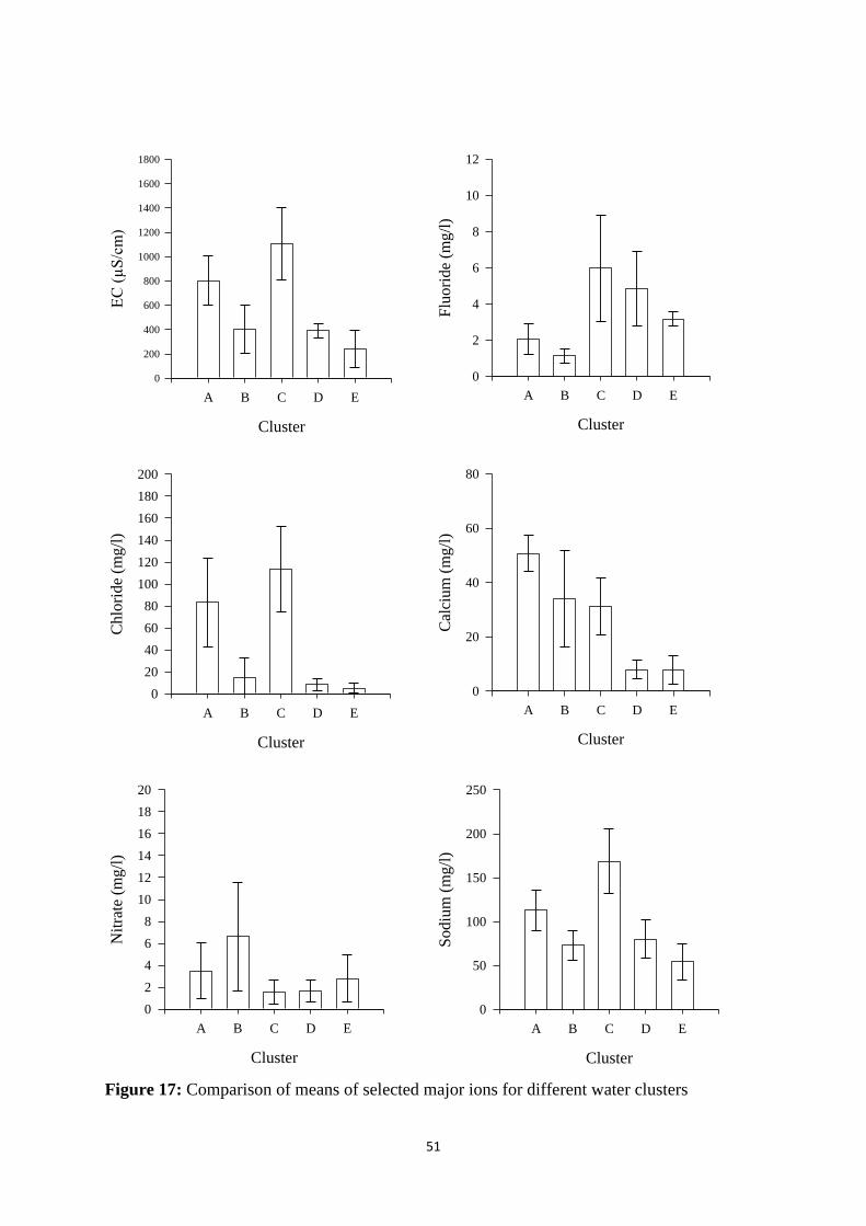
51
Cluster
A B C D E
EC
(µ
S/c
m)
0
200
400
600
800
1000
1200
1400
1600
1800
Cluster
A B C D E
Flu
ori
de
(mg
/l)
0
2
4
6
8
10
12
Cluster
A B C D E
Chlo
ride
(mg/l
)
0
20
40
60
80
100
120
140
160
180
200
Cluster
A B C D E
Cal
ciu
m (
mg
/l)
0
20
40
60
80
Cluster
A B C D E
Nit
rate
(m
g/l
)
0
2
4
6
8
10
12
14
16
18
20
Cluster
A B C D E
Sodiu
m (
mg/l
)
0
50
100
150
200
250
Figure 17: Comparison of means of selected major ions for different water clusters
52
3.5.3 Spatial distributions of nitrate, sulphate and chloride
Nitrate and other nutrients are amongst the best indicators of anthropogenic influence in
groundwater quality assessment (Kaown et al., 2009). Apart from on-site sanitation practice
in the research area, urban agriculture and animal husbandry are also common. All these are
likely to threaten the quality of groundwater for various uses including drinking and other
domestic purposes. The chances of pollutants to be released and transported from these
anthropogenic sources to the shallow aquifers are very high (Drechsel & Dongus, 2010).
Very low concentrations of nitrate, chloride and sulphate were observed in groundwater
samples collected from northern part of the study area (Appendix 1). This suggests the
influence of natural sources such as nitrogen leached from natural soils, volcanic minerals
(e.g., apatite) and gases rather than anthropogenic activities. However, high concentrations of
NO3-, Cl
- and SO4
2- were observed in wells and springs (Appendix 1) located in highly
populated urban areas (South of the study area) where the use of pit latrine and soak away pit
as sanitary facilities is common. Additionally, effluent from a combined domestic and
industrial wastewater treatment plant (waste stabilization ponds) is being used for irrigation
purpose in southern part of the study area which is likely to cause groundwater
contamination. Similar cases of groundwater contamination have been reported in Tanzania
and other parts of the world (Nkotagu, 1996b; Mato & Kaseva, 1999; Kaown et al., 2009;
Elisante & Muzuka, 2015). In most cases, these wastes are discharged haphazardly to the
environment (Couth & Trois, 2011; Laramee & Davis, 2013) or due to underground leakage
from pit latrine, septic tanks and soak-away pit which are common sanitary facilities in the
study area and Tanzania at large (Chaggu et al., 2002; Jenkins et al., 2014). Moreover, water
samples collected from northwest and western part of the study area commonly known as
Ngaramtoni and Magereza showed relatively high concentrations of both Cl─ and SO4
2─
(Appendix 1). The area is dominated by cultivation of coffee, wheat, sunflower, maize, and
beans. Therefore, fertilizer application and uncontrolled waste disposal mainly domestic
sewage may have also contributed to these constituents in groundwater. Generally, the quality
of groundwater with respect to NO3-, Cl
- and SO4
2- in the study area was generally good as
the concentrations are still fairly below the recommended WHO guidelines with exception of
samples S04, S05 and W20 which recorded high nitrate levels 17.3, 10.9 and 10.1 mg/l
respectively possibly caused by human activities.

53
3.6 Conclusions
The hydrogeochemical assessment results and distribution of groundwater major cations
(Na+, Ca
2+, K
+, Mg
2+) and anions (HCO3
-, Cl
-, SO4
2-, F
-) in the study area indicate that
groundwater chemistry is mainly influenced by aquifer lithology than anthropogenic
activities. Groundwater in the study area is dominated by sodium and bicarbonate ions which
define the general composition of the water type to be Na-K-HCO3. With exception of
fluoride and faecal contamination (not covered in this study) the quality of groundwater is
generally suitable for drinking purpose and other socio-economic uses. Based on the
hydrogeological investigation, two potential aquifers (volcanic sediment and
weathered/fractured formation) have been identified both having substantial yield. Generally,
the aquifers yield water containing significant concentration of fluoride exceeding WHO
guidelines. Eighty two (82) percent of the analyzed groundwater samples indicated fluoride
concentrations higher than WHO guidelines and Tanzanian drinking water standards (1.5
mg/l). The northern and northwestern parts of the study area indicated high fluoride
concentrations in both well and spring waters than southern zone. As mentioned earlier, high
fluoride concentration in northern and northwestern parts is probably due to dominance in
basaltic formation and other fluoride rich volcanic materials such as lahars and volcanic ash
which are known to contain and release significant amount of fluoride into groundwater in
the region. However, a detailed geological studies need to be conducted to precisely inform
the entire spectrum of fluoride distribution in the study area. Groundwater abstracted from the
southern part of the study area is of better quality for human consumption than northern
zones which is at high elevation on the foot of Mt. Meru. The influence of anthropogenic
pollutants was observed in shallow wells and spring sources. This was evidenced by
relatively high concentrations of nitrate, chloride and sulphate in samples collected from
sources close to populated urban areas, wastewater effluent disposal zones, and croplands.
Spring water sources should be protected from anthropogenic activities as they produce water
of good quality in terms of key chemical parameters including fluoride which seems to be
critical in the study area.

54
CHAPTER FOUR
GROUNDWATER ABSTRACTION AND AQUIFER SUSTAINABILITY IN
ARUSHA WELLFIELD
Abstract
Groundwater discharges and drawdown measurements (2000-2016) from production wells in
combination with climate data were considered to establish groundwater abstraction trends
and possible impacts in Arusha wellfield. The findings revealed significant groundwater
reserve depletion in the wellfield. Water level decline of about 1.0 m per year and reduction
in well discharges of about 20 to 61% were observed from existing production wells for a
period not exceeding 17 years. The results suggest that the Arusha wellfield is experiencing
groundwater storage depletion which is partly due to over-abstraction and reduced
groundwater recharge. Based on the available borehole data groundwater abstraction from
Arusha wellfield was estimated to be 13 254 719 m3/year which is far less than the current
water demand (34x106 m
3/year). However, this amount is less than the actual amount of
groundwater abstracted as most individual wells are drilled without getting water use permit.
The groundwater recharge was estimated to 13 035 880 m3/year which is higher than
estimated abstracted amount but less than the current city water demand. This indicates that
the wellfield is already stressed due to groundwater over-abstraction. There is also evidence
of decreasing rainfall amount and increasing temperature as a result of climate change which
may contribute to groundwater depletion in the region. The quality of groundwater notably
level of fluoride has significantly increased in some production wells to the extent of
abandoning them from public water supply system.
Keywords: Groundwater abstraction, wellfield, groundwater recharge
55
4.1 Introduction
Groundwater has been used globally as a reliable source of water supply as surface water is
facing a number of challenges and therefore, not a reliable and dependable source in terms of
quality and quantity at any one time (Mato, 2002; Lu et al., 2015). Groundwater is not easily
affected by impact of climate variability such as prolonged drought which is seriously
affecting surface water resources such as rivers and streams (Taylor et al., 2013; Chang et al.,
2015). Furthermore, groundwater is not as vulnerable to pollution as surface water sources.
Hence, it requires less treatment effort prior human consumption. Because of advantage of
groundwater resource being less vulnerable to pollution and can be available in most places
worldwide its exploitation has been tremendously increasing globally in both humid and
semi-arid regions. Intensive groundwater abstraction has been reported in different parts of
the world including Europe, China, United States of America, Iran, India, and Pakistan
(Wada et al., 2010). According to China‘s agenda 21 of 1994 about two-thirds of cities in
China depend on groundwater for urban water supply (Wu et al., 2009). Despite having many
surface water resources in Tanzania such as large freshwater lakes and rivers, groundwater
has been playing crucial role in both domestic and irrigation supplies. The rural areas and
major towns and municipalities in central and northern regions which are characterized by
semi-arid climate depend largely on groundwater abstraction as the main source of water
supply (Kashaigili, 2010; Taylor et al., 2013). Arusha where the current study was conducted
is one of the regions which depend largely on groundwater as the main source of water
supply. Other regions include Dodoma, Singida and Kilimanjaro (Kashaigili, 2010). Despite
the availability of groundwater potential, its quality which may be influenced by both natural
and anthropogenic factors dictates the level of development and its uses.
Increasing groundwater exploitation has many side effects including groundwater storage
depletion, land subsidence, salt water intrusion and general water quality degradation, and
aquatic life distortion in riparian zones and wetlands. The impacts of groundwater over-
abstraction may be minimized by a proper planning and rational utilization of the resource.
Therefore, sustainable management of this resource is dependent on better knowledge of the
groundwater recharge potential, abstraction rate and hydrogeochemical evolution. It should
however, be noted that groundwater development in Arusha like many other places in
Tanzania is not adequately controlled (Kashaigili, 2010; GITEC & WEMA, 2011; Mtoni et
al., 2013). In most cases, borehole drilling especially by private companies or individuals is
carried out sometimes without getting permission from responsible water resources

56
management authority as a result the amount of groundwater abstracted from the wellfield is
not known. The practice has led into an alarming situation for those wells with some
monitoring data. Among the reported issues are groundwater level decline and subsequent
decrease in well discharges. The situation is likely to skyrocket the pumping costs as well as
water scarcity due to rapid population growth accompanied by increase in socio economic
activities which require more water. The situation if prolonged is expected to cause more
serious effects not only in aquifers but also in wetlands, natural spring and river flows
including aquatic ecosystem.
More than 400 wells (shallow and deep) have been drilled in the wellfield without proper
planning and the abstracted groundwater amount is not known. Therefore, this study is
aiming at establishing groundwater abstraction and water level (drawdown) trends from
existing production wells as preliminary assessment for rational groundwater resource
management. The study further aimed to determine the groundwater recharge and current
abstraction impacts for sustainable water resource utilization.
4.2 Materials and Methods
4.2.1 Mapping of wells
The description of the study area is covered in chapter 3. Both individual and wells used for
public water supply were considered in groundwater investigation (Fig. 18). During
fieldwork that was conducted from 2015 to 2016, well mapping, discharge and drawdown
measurements were carried out from existing production wells. Discharge and drawdown
measurements could be possible only in wells used for public water supply. These wells were
properly constructed and allow measurements of important hydraulic parameters for
monitoring purposes which is not the case for individual owned wells. Apart from data
collected during fieldwork, monitoring data for few wells from 2000 to 2014 were obtained
from AUWSA and considered for groundwater investigation.
The data collected include lithology, well completion details and location coordinates using a
hand-held global positioning system (GPS), GARMIN GPSmap62S. Addition list of well
inventory conducted in 2013 in the study area were obtained from Pangani basin water office,
a government agency responsible for water resources management at basin level. Most of
these wells lacked almost all technical information such as hydrogeological aspect. However,

57
the inventory provided other details such as type of well (deep or shallow), coordinates,
operational status and intended use.

58
Figure 18: Groundwater development in Arusha wellfield

59
4.2.2 Well discharge measurements
Flow Meter, discharge measurements were obtained direct from the flow meter installed in
well heads. The readings were taken every twenty four (24) hours or less whenever there was
power interruption. When there was no power interruption, most of the wells used for public
water supply were operated for 24 hours a day.
Indirect method, this approach was based on pumping rate and water consumption mainly
governed by the use of water. The approach gave an average well discharge for a particular
use. The pumping frequency was determined by available storage capacity and water
consumption rate. For unknown pumping time, well discharge was estimated first by
establishing water consumption for a particular use and respective storage period. In most
cases, the storage volume or container was known as well as storage period. This method was
applied to estimate well discharge for individual wells mainly owned by households, hotels,
bars or restaurants, and car wash services.
4.2.3 Water level measurements
Drawdown measurements were possible only for wells with deeper line installation. The
deeper line is installed inside the well casing to enable the water level meter into the well
without being obstructed from electrical or other cables connected to the submersible pump.
The drawdown readings were always taken while the pump was running as most wells
operate for 24 hours a day. The water level was measured with reference from the ground
surface in meters.
4.2.4 Groundwater recharge estimation
The groundwater recharge mechanism in the study area was considered to be due to direct
infiltration from rainfall. The current study adopted the groundwater recharge rate (114.4
mm/year) established by GITEC & WEMA (2011) in a study titled ―Groundwater assessment
of the Pangani basin in Tanzania‖. The recharge rate was calculated from the output of a
computer-based Thornwaite Mather Water balance (TMWB) model. The TMWB model
performs water balance problem based on long term average monthly precipitation, potential
evapotranspiration, latitudes, soil properties and vegetation characteristics. In the study area,
the recharge is likely to take place during long rains period starting from March to May
where there is surplus for groundwater recharge.
60
4.3 Results
4.3.1 Mapping of wells
A total of 393 shallow and deep wells were considered in groundwater abstraction
investigation in the study area (Fig. 18). Only 8% are registered and have water use permits
which are statutorily issued by Ministry of Water through Pangani basin water board
(PBWB). The rest of groundwater development and abstraction is carried out without
following proper procedures as stipulated in Water Resources Management Act of 2009.
Furthermore, those unregistered wells have no technical information documented to allow
proper groundwater monitoring and management follow up.
4.3.2 Well discharge trend
Table 10 summarises well discharge data for thirteen (13) deep wells in Arusha wellfield
from 2000 to 2016. A continuous decrease in well discharges has been observed in almost all
wells in the wellfield (Figs. 19 through 28). Pumping has been conducted continuously and
monitoring data could be obtained only from few production wells owned by AUWSA. The
decrease in well discharge varies from one location to the other. The wellfield was divided
into five different blocks based on the topography and proximity. The blocks and respective
wells into brackets include Kiranyi (W15 and W18), Lorovani (W11 and W14), Sanawari
(W07, W10 and W22) Ilboru (W12 and W19) and Emco (W04) (Fig. 9). In Kiranyi block, the
discharge has declined for about 46% while in Sakina it has declined by 35% (Figs. 19 and
20) for the last seventeen (17) years period. In Lorovani block, two production wells were
considered and observed to have a discharge drop of about 16% and 26% for Lorovani
Bondeni (Fig. 21) and Lorovani yard (Fig. 22) respectively. This block was observed to
experience less decrease in discharge compared to other blocks in the study area. Sanawari
block that had three production wells showed a drop in well discharge of more than 50% for
the last 17 years. Figures 23 through 25 show the decrease in well discharges of 27%, 50%
and 57% for Sanawari P/S, Old Sanawari and Moivo II respectively. This block has recorded
the highest discharge drop in the study area. The hydrographs in Ilboru block indicated
abnormal trends and according to AUWSA personal communication (2015), the trend is
probably due to power fluctuations (low voltage) and missing data in the area (Figs. 26 and
27). Emco is another block located in southern part of the study area and only single well had
discharge records for consideration. Similarly, the well showed a discharge drop of about
19% (Fig. 28). Based on the spatial distribution of investigated wells and trends of well
61
discharges, it is evident that groundwater reserve in Arusha city is continuously being
depleted.
4.3.3 Water level trend
The drawdown measurements were only possible for three wells while others had no reliable
data for consideration. The drawdown from Oltulelei well has increased from 100.3 to 113.8
m. This is a water level decline of about 11.9% (Fig. 29) for the past 16 years time period
accompanied by decrease in well discharge of about 12.5% from 215 to 180 m3/h (Table 10).
Mianzini well which is also under the same block indicated water level decline of about 1.3
m for the measurements conducted between September 2015 and September 2016. The well
lacks previous records which could be used to establish water level trends. Sanawari P/S well
indicated 15.5 m water level decline (14.7%) since 2001 to date (Fig. 30). However, there is a
missing data between 2010 and 2015. Other wells have neither records nor provision for
taking drawdown measurements but they have significant decrease in discharges as shown in
Table 10.
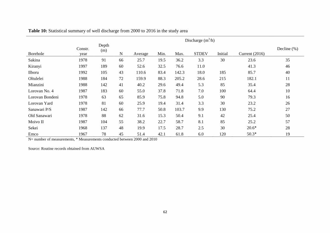
62
Table 10: Statistical summary of well discharge from 2000 to 2016 in the study area
Discharge (m3/h)
Decline (%)
Borehole
Constr.
year
Depth
(m) N Average Min. Max. STDEV Initial Current (2016)
Sakina 1978 91 66 25.7 19.5 36.2 3.3 30 23.6 35
Kiranyi 1997 189 60 52.6 32.5 76.6 11.0
41.3 46
Ilboru 1992 105 43 110.6 83.4 142.3 18.0 185 85.7 40
Oltulelei 1988 184 72 159.9 88.3 205.2 28.6 215 182.1 11
Mianzini 1988 142 41 40.2 29.6 49.4 5.3 85 35.4 28
Lorovan No. 4 1987 183 60 55.0 37.8 71.8 7.0 100 64.4 10
Lorovan Bondeni 1978 63 65 85.9 75.8 94.8 5.0 90 79.3 16
Lorovan Yard 1978 81 60 25.9 19.4 31.4 3.3 30 23.2 26
Sanawari P/S 1987 142 66 77.7 50.8 103.7 9.9 130 75.2 27
Old Sanawari 1978 88 62 31.6 15.3 50.4 9.1 42 25.4 50
Moivo II 1987 104 55 38.2 22.7 58.7 8.1 85 25.2 57
Sekei 1968 137 48 19.9 17.5 28.7 2.5 30 20.6* 28
Emco 1967 78 45 51.4 42.1 61.8 6.0 120 50.3* 19
N= number of measurements, * Measurements conducted between 2000 and 2010
Source: Routine records obtained from AUWSA
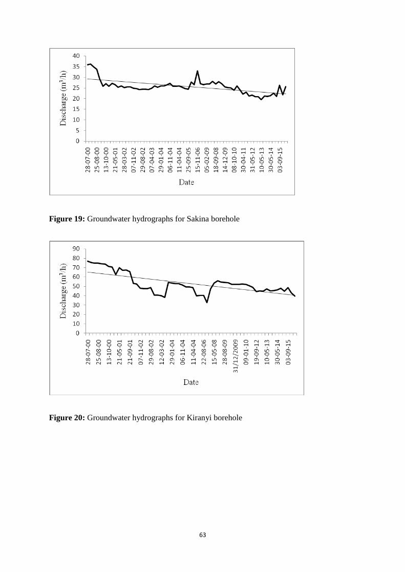
63
Figure 19: Groundwater hydrographs for Sakina borehole
Figure 20: Groundwater hydrographs for Kiranyi borehole
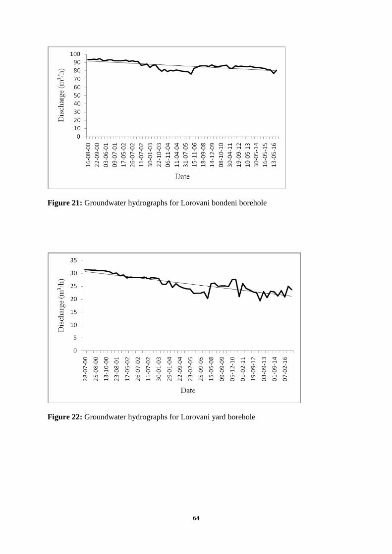
64
Figure 21: Groundwater hydrographs for Lorovani bondeni borehole
Figure 22: Groundwater hydrographs for Lorovani yard borehole

65
Figure 23: Groundwater hydrographs for Sanawari P/S borehole
Figure 24: Groundwater hydrographs for Old Sanawari borehole

66
Figure 25: Groundwater hydrographs for Moivo II borehole
Figure 26: Groundwater hydrographs for Ilboru borehole
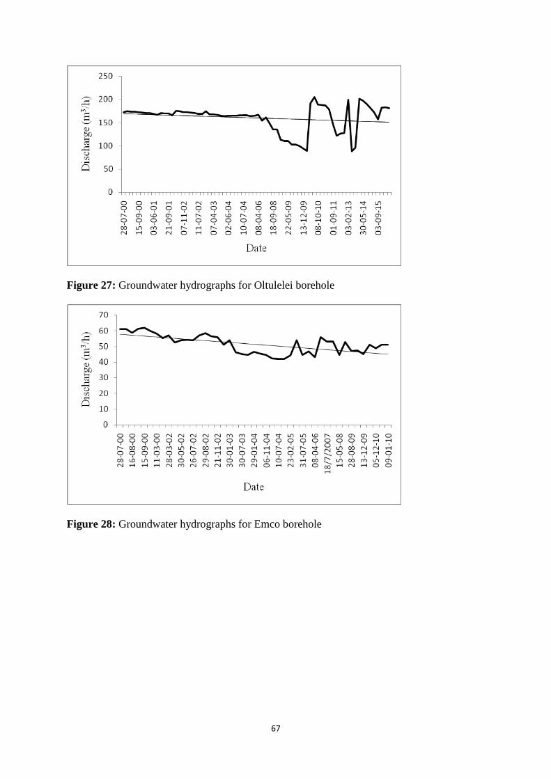
67
Figure 27: Groundwater hydrographs for Oltulelei borehole
Figure 28: Groundwater hydrographs for Emco borehole
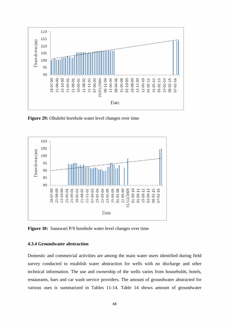
68
Figure 29: Oltulelei borehole water level changes over time
Figure 30: Sanawari P/S borehole water level changes over time
4.3.4 Groundwater abstraction
Domestic and commercial activities are among the main water users identified during field
survey conducted to establish water abstraction for wells with no discharge and other
technical information. The use and ownership of the wells varies from households, hotels,
restaurants, bars and car wash service providers. The amount of groundwater abstracted for
various uses is summarized in Tables 11-14. Table 14 shows amount of groundwater
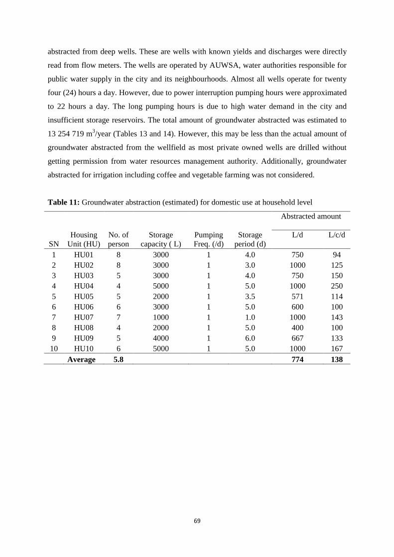
69
abstracted from deep wells. These are wells with known yields and discharges were directly
read from flow meters. The wells are operated by AUWSA, water authorities responsible for
public water supply in the city and its neighbourhoods. Almost all wells operate for twenty
four (24) hours a day. However, due to power interruption pumping hours were approximated
to 22 hours a day. The long pumping hours is due to high water demand in the city and
insufficient storage reservoirs. The total amount of groundwater abstracted was estimated to
13 254 719 m3/year (Tables 13 and 14). However, this may be less than the actual amount of
groundwater abstracted from the wellfield as most private owned wells are drilled without
getting permission from water resources management authority. Additionally, groundwater
abstracted for irrigation including coffee and vegetable farming was not considered.
Table 11: Groundwater abstraction (estimated) for domestic use at household level
SN
Housing
Unit (HU)
No. of
person
Storage
capacity ( L)
Pumping
Freq. (/d)
Storage
period (d)
Abstracted amount
L/d L/c/d
1 HU01 8 3000 1 4.0 750 94
2 HU02 8 3000 1 3.0 1000 125
3 HU03 5 3000 1 4.0 750 150
4 HU04 4 5000 1 5.0 1000 250
5 HU05 5 2000 1 3.5 571 114
6 HU06 6 3000 1 5.0 600 100
7 HU07 7 1000 1 1.0 1000 143
8 HU08 4 2000 1 5.0 400 100
9 HU09 5 4000 1 6.0 667 133
10 HU10 6 5000 1 5.0 1000 167
Average 5.8
774 138
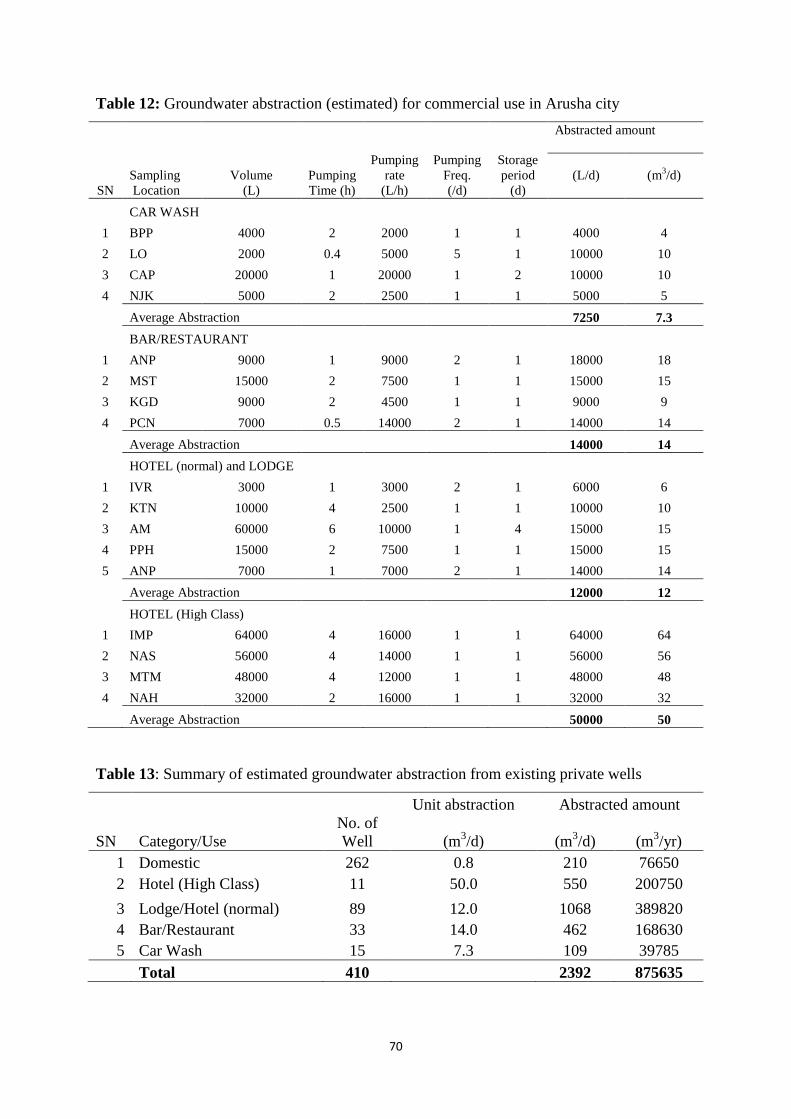
70
Table 12: Groundwater abstraction (estimated) for commercial use in Arusha city
SN
Sampling
Location
Volume
(L)
Pumping
Time (h)
Pumping
rate
(L/h)
Pumping
Freq.
(/d)
Storage
period
(d)
Abstracted amount
(L/d) (m3/d)
CAR WASH
1 BPP 4000 2 2000 1 1 4000 4
2 LO 2000 0.4 5000 5 1 10000 10
3 CAP 20000 1 20000 1 2 10000 10
4 NJK 5000 2 2500 1 1 5000 5
Average Abstraction
7250 7.3
BAR/RESTAURANT
1 ANP 9000 1 9000 2 1 18000 18
2 MST 15000 2 7500 1 1 15000 15
3 KGD 9000 2 4500 1 1 9000 9
4 PCN 7000 0.5 14000 2 1 14000 14
Average Abstraction
14000 14
HOTEL (normal) and LODGE
1 IVR 3000 1 3000 2 1 6000 6
2 KTN 10000 4 2500 1 1 10000 10
3 AM 60000 6 10000 1 4 15000 15
4 PPH 15000 2 7500 1 1 15000 15
5 ANP 7000 1 7000 2 1 14000 14
Average Abstraction
12000 12
HOTEL (High Class)
1 IMP 64000 4 16000 1 1 64000 64
2 NAS 56000 4 14000 1 1 56000 56
3 MTM 48000 4 12000 1 1 48000 48
4 NAH 32000 2 16000 1 1 32000 32
Average Abstraction
50000 50
Table 13: Summary of estimated groundwater abstraction from existing private wells
Unit abstraction Abstracted amount
SN Category/Use
No. of
Well (m3/d) (m
3/d) (m
3/yr)
1 Domestic 262 0.8 210 76650
2 Hotel (High Class) 11 50.0 550 200750
3 Lodge/Hotel (normal) 89 12.0 1068 389820
4 Bar/Restaurant 33 14.0 462 168630
5 Car Wash 15 7.3 109 39785
Total 410
2392 875635
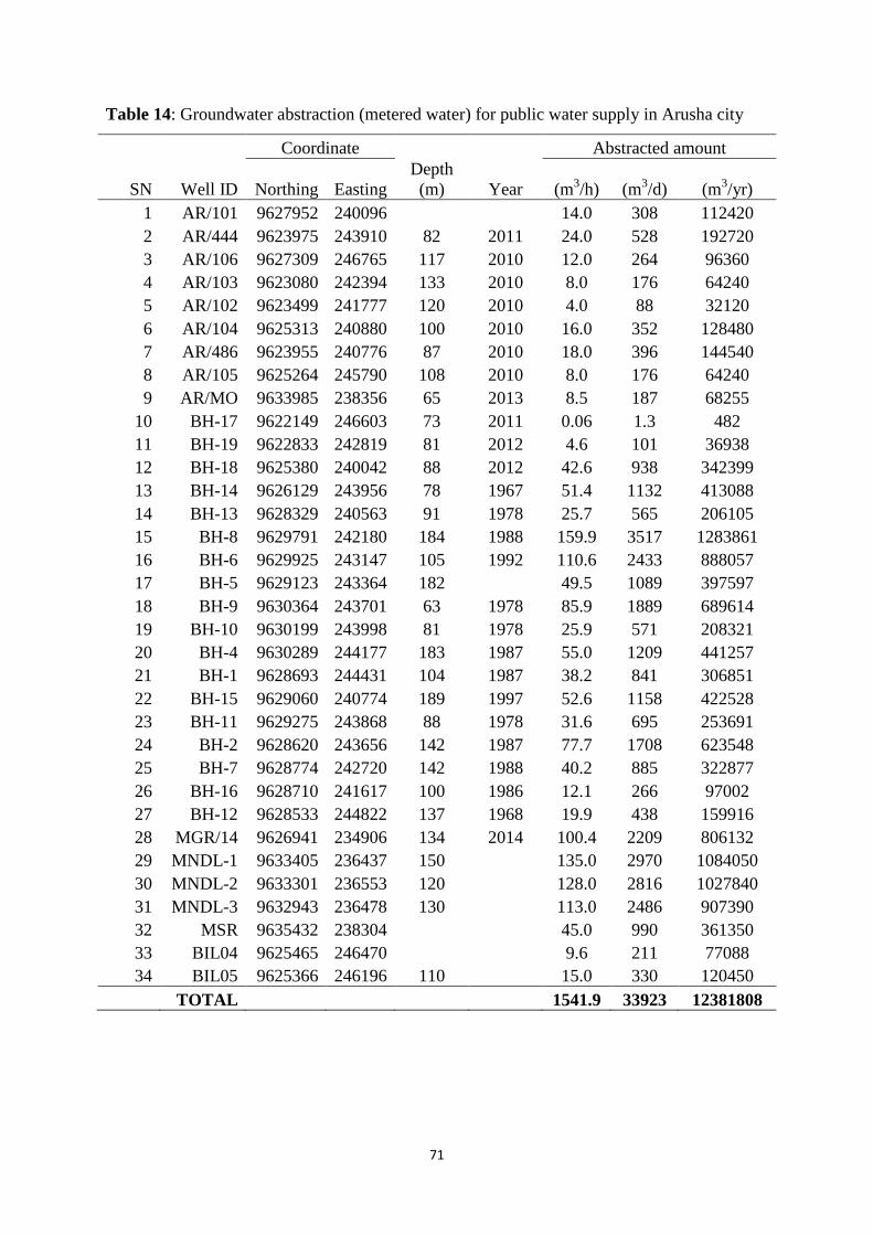
71
Table 14: Groundwater abstraction (metered water) for public water supply in Arusha city
Coordinate Abstracted amount
SN Well ID Northing Easting
Depth
(m) Year (m3/h) (m
3/d) (m
3/yr)
1 AR/101 9627952 240096
14.0 308 112420
2 AR/444 9623975 243910 82 2011 24.0 528 192720
3 AR/106 9627309 246765 117 2010 12.0 264 96360
4 AR/103 9623080 242394 133 2010 8.0 176 64240
5 AR/102 9623499 241777 120 2010 4.0 88 32120
6 AR/104 9625313 240880 100 2010 16.0 352 128480
7 AR/486 9623955 240776 87 2010 18.0 396 144540
8 AR/105 9625264 245790 108 2010 8.0 176 64240
9 AR/MO 9633985 238356 65 2013 8.5 187 68255
10 BH-17 9622149 246603 73 2011 0.06 1.3 482
11 BH-19 9622833 242819 81 2012 4.6 101 36938
12 BH-18 9625380 240042 88 2012 42.6 938 342399
13 BH-14 9626129 243956 78 1967 51.4 1132 413088
14 BH-13 9628329 240563 91 1978 25.7 565 206105
15 BH-8 9629791 242180 184 1988 159.9 3517 1283861
16 BH-6 9629925 243147 105 1992 110.6 2433 888057
17 BH-5 9629123 243364 182
49.5 1089 397597
18 BH-9 9630364 243701 63 1978 85.9 1889 689614
19 BH-10 9630199 243998 81 1978 25.9 571 208321
20 BH-4 9630289 244177 183 1987 55.0 1209 441257
21 BH-1 9628693 244431 104 1987 38.2 841 306851
22 BH-15 9629060 240774 189 1997 52.6 1158 422528
23 BH-11 9629275 243868 88 1978 31.6 695 253691
24 BH-2 9628620 243656 142 1987 77.7 1708 623548
25 BH-7 9628774 242720 142 1988 40.2 885 322877
26 BH-16 9628710 241617 100 1986 12.1 266 97002
27 BH-12 9628533 244822 137 1968 19.9 438 159916
28 MGR/14 9626941 234906 134 2014 100.4 2209 806132
29 MNDL-1 9633405 236437 150
135.0 2970 1084050
30 MNDL-2 9633301 236553 120
128.0 2816 1027840
31 MNDL-3 9632943 236478 130
113.0 2486 907390
32 MSR 9635432 238304
45.0 990 361350
33 BIL04 9625465 246470
9.6 211 77088
34 BIL05 9625366 246196 110
15.0 330 120450
TOTAL
1541.9 33923 12381808

72
4.3.5 Current water demand
Arusha city has households of different income as well as living standards ranging from
lower to higher income. Estimation of water supply requirements or demand is governed by
the living standard of the community and types of sanitation systems used. In case of Arusha
city the medium income category was considered as an average representing majority of the
city population. The common sanitation systems in the study area are septic tank connected
to soak away pit, pour flush toilets and traditional pit latrines. Only small area (7 %) of the
city is covered by sewerage network. Generally, the study area is considered as medium
income area which requires 110 litres of water for every person per day (Table 15). Based on
forecasted population to the year 2016 with annual growth rate of 2.7 % (URT, 2013), the
population is about 845 030 inhabitants. This population requires about 92 953 300 l/d
equivalent to 34x106 m
3/yr.
Table 15: Urban area water requirements (l/c/d)
Consumer category FR M-UT M-PBT Remarks
Low income using
kiosks or public taps
25 25 25 Most squatter areas, to be taken as
the minimum
Low income multiple
household with Yard
Tap
50 45 40 Low income group housing No
inside installation and pit latrine
Low income, single
household with Yard
Tap
70 60 50 Low income group housing No
inside installation and pit latrine
Medium Income
Household
130 110 90 Medium income group housing,
with sewer or septic tank
High Income
Household
250 200 150 High income group housing, with
sewer or septic tank
FR = flat rate, M-UT = metered with uniform tariff, M-PBT = metered with progressive tariff
Source: URT (2009)
73
4.3.6 Groundwater recharge
According to GITEC & WEMA (2011), the estimated annual recharge rate using
Thornthwaite Monthly Water-Balance (TMWB) model is 114.4 mm. This information was
derived from 40 years weather data collected in the study area. The potential groundwater
recharge area is considered to be in high elevations on the slopes of Mt. Meru where faults
and structures have been observed (Ghiglieri et al., 2010). Figure 31 depicts delineated
potential recharge area for Arusha wellfield which is estimated to 113.95 km2. Only the area
at the northern part of the study area located on the southern slopes of Mt. Meru was
considered as it has been reported in previous works as potential recharge area in the region
(Ghiglieri et al., 2008, 2010; Ong‘or & Long-cang, 2007). The product of estimated recharge
rate and potential recharge area of the wellfield gives a total annual recharge of 13 035 880
m3/year. This excludes induced recharge from adjacent aquifers and nearby surface water
bodies. Additionally, leakages from water supply networks and sewage disposal facilities
may also contribute to groundwater recharge.
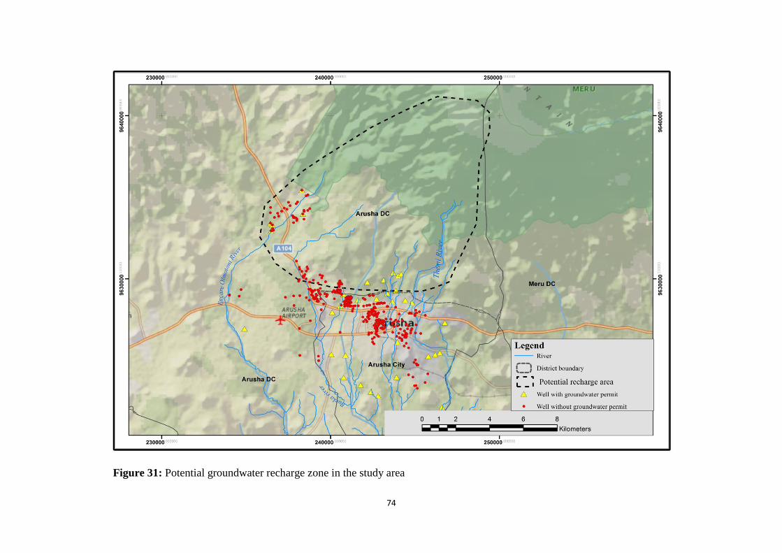
74
Figure 31: Potential groundwater recharge zone in the study area
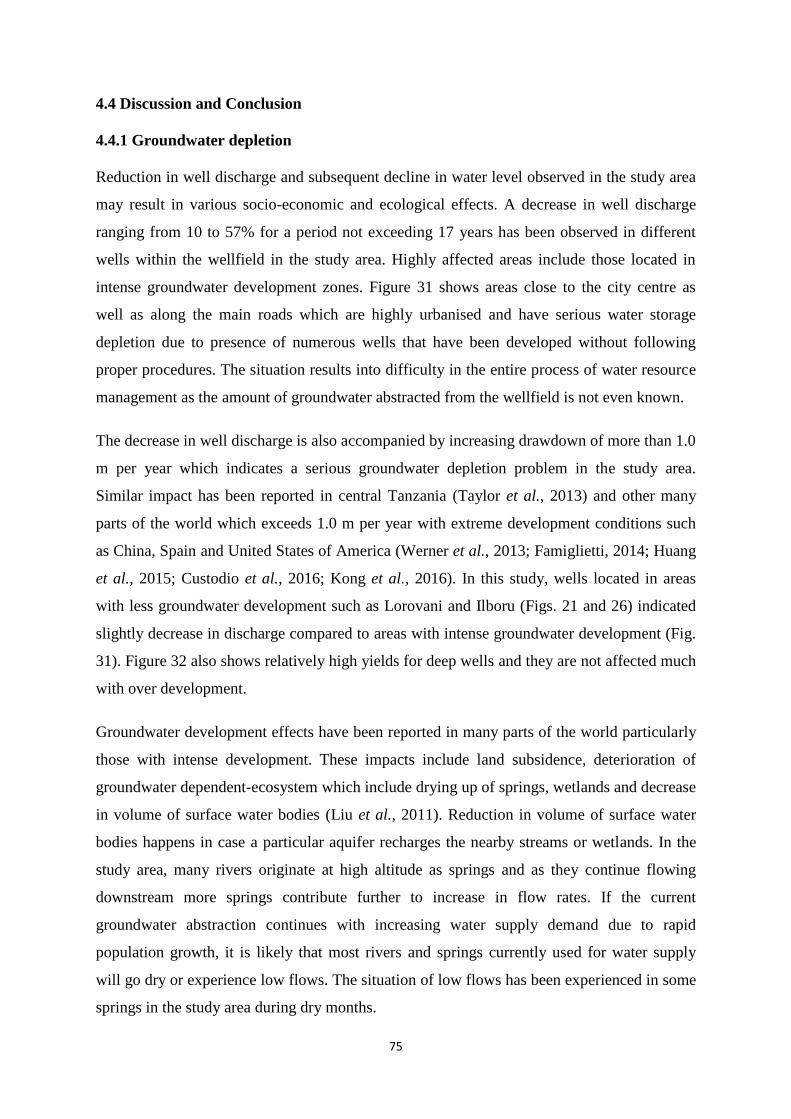
75
4.4 Discussion and Conclusion
4.4.1 Groundwater depletion
Reduction in well discharge and subsequent decline in water level observed in the study area
may result in various socio-economic and ecological effects. A decrease in well discharge
ranging from 10 to 57% for a period not exceeding 17 years has been observed in different
wells within the wellfield in the study area. Highly affected areas include those located in
intense groundwater development zones. Figure 31 shows areas close to the city centre as
well as along the main roads which are highly urbanised and have serious water storage
depletion due to presence of numerous wells that have been developed without following
proper procedures. The situation results into difficulty in the entire process of water resource
management as the amount of groundwater abstracted from the wellfield is not even known.
The decrease in well discharge is also accompanied by increasing drawdown of more than 1.0
m per year which indicates a serious groundwater depletion problem in the study area.
Similar impact has been reported in central Tanzania (Taylor et al., 2013) and other many
parts of the world which exceeds 1.0 m per year with extreme development conditions such
as China, Spain and United States of America (Werner et al., 2013; Famiglietti, 2014; Huang
et al., 2015; Custodio et al., 2016; Kong et al., 2016). In this study, wells located in areas
with less groundwater development such as Lorovani and Ilboru (Figs. 21 and 26) indicated
slightly decrease in discharge compared to areas with intense groundwater development (Fig.
31). Figure 32 also shows relatively high yields for deep wells and they are not affected much
with over development.
Groundwater development effects have been reported in many parts of the world particularly
those with intense development. These impacts include land subsidence, deterioration of
groundwater dependent-ecosystem which include drying up of springs, wetlands and decrease
in volume of surface water bodies (Liu et al., 2011). Reduction in volume of surface water
bodies happens in case a particular aquifer recharges the nearby streams or wetlands. In the
study area, many rivers originate at high altitude as springs and as they continue flowing
downstream more springs contribute further to increase in flow rates. If the current
groundwater abstraction continues with increasing water supply demand due to rapid
population growth, it is likely that most rivers and springs currently used for water supply
will go dry or experience low flows. The situation of low flows has been experienced in some
springs in the study area during dry months.
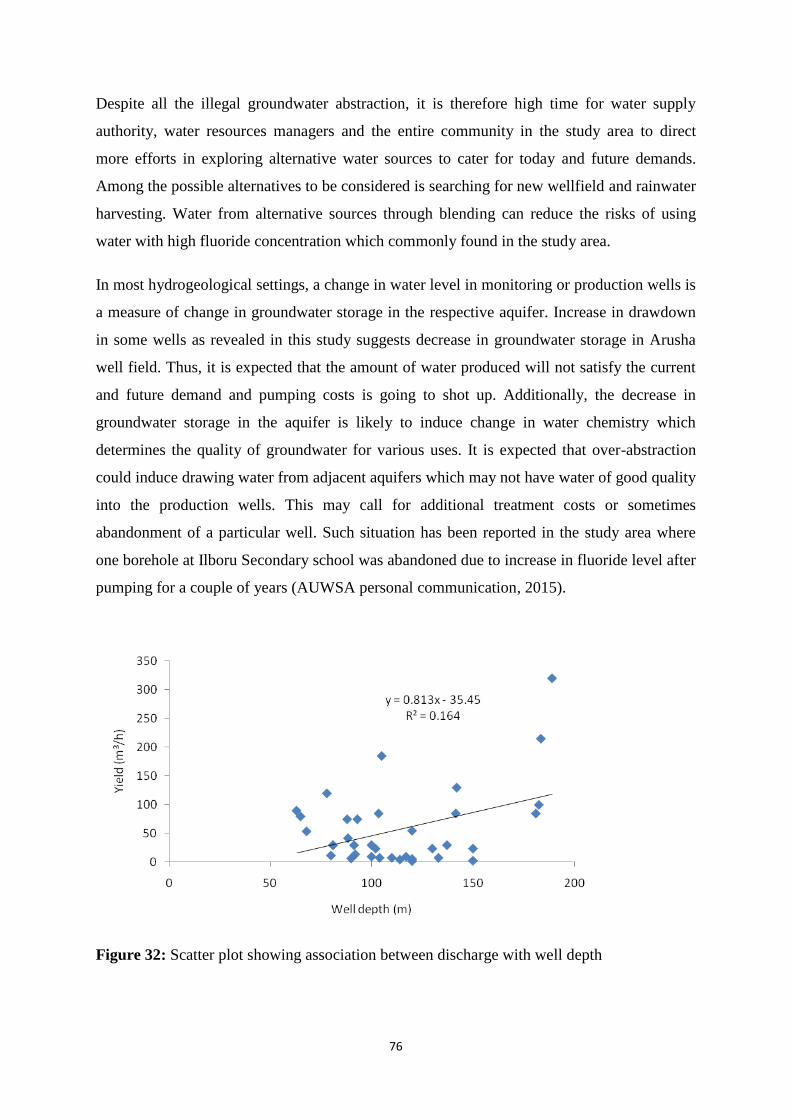
76
Despite all the illegal groundwater abstraction, it is therefore high time for water supply
authority, water resources managers and the entire community in the study area to direct
more efforts in exploring alternative water sources to cater for today and future demands.
Among the possible alternatives to be considered is searching for new wellfield and rainwater
harvesting. Water from alternative sources through blending can reduce the risks of using
water with high fluoride concentration which commonly found in the study area.
In most hydrogeological settings, a change in water level in monitoring or production wells is
a measure of change in groundwater storage in the respective aquifer. Increase in drawdown
in some wells as revealed in this study suggests decrease in groundwater storage in Arusha
well field. Thus, it is expected that the amount of water produced will not satisfy the current
and future demand and pumping costs is going to shot up. Additionally, the decrease in
groundwater storage in the aquifer is likely to induce change in water chemistry which
determines the quality of groundwater for various uses. It is expected that over-abstraction
could induce drawing water from adjacent aquifers which may not have water of good quality
into the production wells. This may call for additional treatment costs or sometimes
abandonment of a particular well. Such situation has been reported in the study area where
one borehole at Ilboru Secondary school was abandoned due to increase in fluoride level after
pumping for a couple of years (AUWSA personal communication, 2015).
Figure 32: Scatter plot showing association between discharge with well depth
77
4.4.2 Groundwater recharge
Groundwater recharge due to precipitation infiltration in fractured or faulted formation is the
dominant mechanism in the study area (Ghiglieri et al., 2010). Annual recharge of about 114
mm has been estimated based on 40 years rainfall data in the study area. However, such a
recharge mechanism is being affected by several factors which may lead into decrease in the
estimated recharge amount. These factors include urbanization and climate change
particularly temperature increase (Figs. 33 and 34) and decreasing trends of rainfall pattern
(Figs. 35 through 38) which have already been experienced in Northern Tanzania. This trend
agrees with the observation and prediction pointed out on climate change impacts in Tanzania
(Omambia & Gu, 2010). This gives a bad signal to the sustainability of the Arusha wellfield
as the demand for water supply is going up from year to year due to rapid population growth
reported in the study area reaching 2.7% annually (URT, 2013).
Figure 33: Average maximum temperature trend from 1973 to 2013, Arusha Airport MET
station (TMA, 2013)

78
Figure 34: Average maximum temperature trend from 1973 to 2013, Kilimanjaro
International Airport MET station (TMA, 2013)
The findings of this study (Chapter 5) has also revealed abstraction of relatively old
groundwater (~ 1400 years BP) from deep wells which is quite long period of time for a
depleted aquifer to replenish the abstracted water. Additionally, urbanization has been
expanding towards the delineated recharge zone in the study area. This involves clearing of
natural vegetation and increasing surface pavements and subsequently reduction in amount of
rainfall infiltrating to the water table (Zipper et al., 2017). However, in other hydrogeological
settings it has been reported that urbanization increases groundwater recharge due to
percolation from septic tank and soak away systems, reduced evapotranspiration as well as
leakages from water and sewerage networks (Naik et al., 2008; Tam & Nga, 2018; Wakode et
al., 2018). But this scenario depends mainly on geology and fundamental hydraulic structure
and properties of the aquifer matrix in the area. Therefore, it is not guaranteed that the
urbanization will counterbalance groundwater recharge due to rainfall infiltration especially
in areas where recharge takes place in fractured and faulted formations like Arusha wellfield.

79
Figure 35: Annual rainfall trend from 1955 to 2013, Arusha Airport MET station (TMA,
2013)
Figure 36: Annual rainfall trend from 1955 to 2013, Arusha Maji MET station (TMA, 2013)

80
Figure 37: Annual rainfall trend from 1955 to 2013, Tengeru MET station (TMA, 2013)
Figure 38: Annual rainfall trend from 1955 to 2013, Kilimanjaro International Airport MET
station (TMA, 2013)
4.4.3 Groundwater abstraction and its impact
Groundwater development which doesn‘t follow or abides to the legal procedures in place is
a threat to the sustainability of the Arusha wellfield. High water level decline and reduced in
well discharge have been observed in most wells (Figs. 19 through 28) located in areas with
intense groundwater abstraction. The amount of groundwater abstracted from more than 90%
of the wells in the wellfield is unknown. The situation is accelerated by the rapid expansion
81
of the city which doesn‘t match with provision of water supply service. Thus, individuals are
forced to drill their own wells sometimes without getting water use permit, the practice which
poses a challenge of controlling the development of groundwater resource in the wellfield. To
the moment it is still unclear the exactly amount of groundwater abstracted as only less than
10% of the wells have water use permit from water resources management authority. The
permit specifies the use and amount of water abstracted from the wellfield which include
drilled wells, springs and rivers. In addition, some individuals have established shallow dug
wells (<15 m deep), this type of development is legally recognized and it is being conducted
without having water use permit. However, the amount of water abstracted is also unknown
as it depends on the intended use. Similarly, other individuals who are not supplied with
water by AUWSA and have not opted for shallow or deep wells they use spring water for
fulfilling their basic needs. Luckily, the area is blessed by having numerous springs with
fresh water scattered all over the wellfield.
To this end, the current groundwater development in the area is likely to alter and affect the
community welfare including groundwater-dependent ecosystems. Now, if the groundwater
development continues with the current practice it will poses serious effects to the Arusha
city. Some of the effects include drying up of springs which supply water to the community
not covered by AUWSA. In addition, reduced spring or river flows will affect water-
dependent ecosystem within and outside the study area particularly downstream of the
catchment. Therefore, urgent management strategy is needed to rescue those impacts likely to
occur as a result of groundwater over-abstraction in the wellfield and surrounding
environments. The needed management strategy will have first to delineate the available
water reserve with respect to present and future water demand for this new and fast growing
touristic city and explore alternative water sources to supplement the already stressed
wellfield. Currently, AUWSA is only able to produce and supply between 35 000 and 60 000
m3/d of water which fluctuates seasonally but the current water demand is 93 000 m
3/d
(AUWSA, 2014). Therefore, majority of the city and its neighbourhoods are not guaranteed
to having safe drinking water instead they get water through their own effort and this
encourages illegal groundwater abstraction hence makes groundwater management difficult.
82
4.5 Conclusion
The Arusha wellfield has been undergoing intensive groundwater development with
abstraction in some cases taking place illegally. The illegal abstraction among other factors
makes groundwater management a challenge in the wellfield. This study is only the first step
towards a comprehensive effort to develop an effective groundwater management strategy for
sustainable water resources utilization in the city and its neighbourhoods to meet the current
and future water needs for socio-economic development as well as ecological functioning.
The findings of this study revealed significant groundwater reserve depletion in the wellfield.
There is a water level decline of about 1.0 m per year. The decline is accompanied by
reduction in well discharges of about 10 to 57% observed from existing production wells for
a period not exceeding 17 years. The decline in water levels and subsequent reduction in
discharges is a result of groundwater over-abstraction and reduced recharge in the area. More
than 90% of individual wells are not registered and were drilled without getting water use
permit from water resources management authority. Therefore, even the amount of
groundwater abstracted is not known which makes a great challenge and difficult in
managing this vital resource.
Areas with larger number of wells experience high level of decrease in well discharge
compared to areas with small number of wells. Based on the available borehole data
groundwater abstraction from Arusha wellfield was estimated to be 13 254 719 m3/year.
However, this amount is less than the actual amount of groundwater abstracted as most
individual wells are drilled without getting water use permit from water resources
management authority. Based on current population, water demand for the entire city and its
neighbourhoods was estimated to 34 000 000 m3/year which is more than twice the estimated
groundwater abstraction from the wellfield. This suggests that majority of the residents are
getting water outside the formal water supply system under AUWSA. The groundwater
recharge was estimated to be 13 035 880 m3/year which is less than both groundwater
discharge from production wells and current water demand. This indicates that the wellfield
is already stressed due to groundwater over-abstraction and calls for water managers to
immediately consider alternative water sources for socio economic development of Arusha
city.
The quality of groundwater notably level of fluoride has significantly increased in some
production wells to the extent of abandoning them from public water supply system. Also

83
some springs within the wellfield have experienced reduction in flows and they are likely to
face further decrease if the current groundwater development practice continues.
Additionally, there is evidence of decreasing rainfall amount in the region as a result of
climate change which may contribute to reduced recharge and subsequently groundwater
depletion. It is also anticipated that water level decline and subsequent reduction in well
discharge will escalate the pumping costs due to increased distance from the water level to
the ground surface.
84
CHAPTER FIVE
GROUNDWATER AGE DATING AND RECHARGE MECHANISM OF ARUSHA
AQUIFER, NORTHERN TANZANIA: APPLICATION OF RADIOISOTOPE AND
STABLE ISOTOPE TECHNIQUES2
Abstract
The continuous abstraction of groundwater from Arusha aquifers in northern Tanzania has
resulted in a decline in water levels and subsequent yield reduction in most production wells.
The situation is threatening sustainability of the aquifers and concise knowledge on the
existing a groundwater challenge is of utmost importance. To gain such knowledge, stable
isotopes of hydrogen and oxygen, and radiocarbon dating on dissolved inorganic carbon
(DIC), were employed to establish groundwater mean residence time and recharge
mechanism.14
C activity of DIC was measured in groundwater samples and corrected using a
δ13
C mixing method prior to groundwater age dating. The results indicated that groundwater
ranging from 1400 years BP to modern is being abstracted from deeper aquifers that are
under intensive development. This implies that the groundwater system is continuously
depleted due to over-pumping, as most of the sampled wells and springs revealed recently
recharged groundwater. High 14
C activities observed in spring water (98.1±7.9 pMC)
correspond with modern groundwater in the study area. The presence of modern groundwater
suggests that shallow aquifers are actively recharged and respond positively to seasonal
variations.
Key words: Groundwater age, radioisotopes, recharge mechanism, Tanzania
2Hydrogeology Journal, https://doi.org/10.1007/s10040-018-1832-0
85
5.1 Introduction
In the city of Arusha, situated in northern Tanzania, groundwater abstracted through drilled
wells and springs is the main source of drinking water supply (GITEC & WEMA, 2011).
Most deep wells with large production volume are located in the central part of the study area
near the foot of Mt. Meru at an elevation from 1400 to 1500 m above sea level (a.s.l.)
(Ong‘or & Long-cang, 2007). According to the Arusha Urban Water Supply and Sanitation
Authority (AUWSA) medium-term strategic plan (2015-2020) report, springs contribute 45%
of the daily water production whereas drilled wells and rivers contribute 37% and 18%
respectively (AUWSA, 2014). However, the proportional contribution from each source
varies depending on season of the year. The seasonal variations mainly affect springs and
rivers by significant reduction in flows during dry periods but production from wells remains
constant (AUWSA, 2014). Generally, water production fluctuates seasonally from an average
of 35 000 m3/d (dry season) to 60 000 m
3/d (rainy season) which is significantly low with
respect to the current water demand (93 270 m3/d) in the city (AUWSA, 2014).
Despite the lack of reliable information on the extent of groundwater abstraction, there is
evidence of groundwater over-pumping in the study area. The decline of water levels (Table
16) and respective yield reduction (Table 17) in wells that have been operational for more
than 20 years has been reported (Ong‘or & Long-cang, 2007; GITEC & WEMA, 2011).
Additionally, an inventory conducted by Pangani Basin Water Office (PBWO) in 2013
revealed more than 400 drilled wells in the study area, most of them unregistered by the
responsible water resources management authority. This suggests that groundwater
abstraction in the area is not adequately controlled to meet the needs of present and future use
(Kashaigili, 2010; Van Camp et al., 2014). However, aquifer storage may be affected by a
number of factors other than groundwater over-pumping (Custodio, 2002). Natural
phenomena, such as delayed and transient effects of the aquifer system, earth quakes, tectonic
movement and climate change, have been reported in many parts of the world with
significant effect in aquifer productivity (Custodio, 2002; Gorokhovich, 2005; Kitagawa et
al., 2006; Kløve et al., 2014; Nigate et al., 2017). Due to the complexity and dynamics of
hydrogeological processes, knowledge of a particular aquifer system including recharge
mechanisms and age of abstracted groundwater is required to inform the cause and extent of
the existing problems. Such a situation leaves a number of questions with respect to
sustainability of groundwater utilization in Arusha City for present and future water resources
development and for avoidance of likely human impacts (drinking water supply) and
86
ecosystem impacts (such as reduced stream flows and springs drying up and subsequent
impacts on aquatic life). The current research was conducted to inform some of the existing
problems or fill knowledge gaps in the study area. Among the issues addressed include
whether groundwater storage depletion is caused by over-pumping or whether the aquifer
system in the study area is not actively recharged.
In order to address some of the experienced groundwater challenges, the study employed the
use of isotopic techniques to investigate the groundwater age and recharge mechanism in the
study area. Currently, there are a number of tracers used for assessment of groundwater
recharge and mean residence time (Chen et al., 2011). These include chlorofluorocarbons
(CFCs), tritium/helium ratio (3H/
3He), krypton-85 (
85Kr) and carbon-14 (
14C) (Douglas et al.
2007; Hoque & Burgess 2012; Sigstedt et al. 2016). Chlorofluorocarbons (CFCs), 3H/
3He and
85Kr are mostly used for tracing young groundwater (< 100 years) (Szabo et al., 1996;
Mathouchanh and Aeschbach-Hertig, 2015). However, this study employed stable isotopes
(hydrogen and oxygen), tritium and 14
C to meet its objectives. The 14
C technique uses the
decay principle of the activity measured in dissolved inorganic carbon (DIC) to estimate the
mean groundwater age of water travelling from the recharge zone to a discharge point along
the flow path (Douglas et al., 2007; Hagedorn, 2015). These techniques have been
undergoing several improvements and are widely used in hydrogeological studies,
particularly groundwater recharge and mean age estimation ranging from young (100 to 1000
years BP) to old groundwater (1000 to millions years) (Bakari et al., 2012b, b; Stewart, 2012;
Gleeson et al., 2016). Despite wide acceptance and global application of isotope techniques,
in Tanzania they have commonly been applied in geology and marine based sediments
studies (Muzuka et al., 2010; Muzuka et al., 2004; Öberg et al., 2013). Conventionally, many
groundwater assessment studies have been focusing on quality issues and leaving aside
aquifer sustainability in terms of potential recharge and groundwater mean residence time
(Ghiglieri et al., 2010; Ghiglieri et al., 2012; Van Camp et al., 2014; Malago et al., 2017).
Lack of such information is likely to threaten sustainability of aquifers under intensive
development (Zongyu et al., 2005).
Thus, this study aimed at establishing groundwater age and recharge mechanism for
sustainable groundwater utilization in Arusha City, using 14
C, tritium and stable isotope (2H
and 18
O) techniques. Isotope composition data have been used for interpretation in

87
conjunction with groundwater physical parameters and some hydrogeological information
which were established during the borehole drilling and construction stage.
Table 16: Water level trends in the study area
Well details Water level (year of measurement) (m b.g.l.)
Location Well
ID
Well depth
(m)
GE
(1988)
HH
(1994)
PBWO
(2006)
GITEC
(2011)
This work
(2016)
Oltulelei W12 184 36.95 58.90 58.90 - 113.77
Ilboru
Sec
W19 105 9.88 17.50 17.50 24.26 -
Ilkloriti W08 182 13.96 33.80 33.80 - -
Moivo II W09 104 2.27 16.60 16.60 27.30 73.43
Mianzini W17 142 14.75 32.20 32.20 30.54 90.54
Abbreviations: GE-Gauff Engineers, HH-Howard Humphreys, PBWB-Pangani Basin Water Board. b.g.l. =
below ground level
Source: GITEC and WEMA (2011)
Table 17: Well discharge trends over time in the study area
Well details Discharge (year of measurement) (m3/h)
Location Well
ID
GE
(1988)
HH
(1994)
PBWO
(2006)
WB
(2010)
GITEC
(2011)
This work
(2016)
Oltulelei W12 264 217.7 164.6 148.3 188.1 182.1
Ilboru Sec W19 220 186.3 128.1 26.5 136 85.7
Ilkloriti W08 150 84.5 - - 52.2 34.6
Sanawari P/S W10 160 - - 91 75 75.2
Moivo II W09 120 120 30.98 38.8 58.2 25.2
Mianzini W17 80 63.9 48.2 49.4 49.4 33.6
Abbreviations: GE-Gauff Engineers, HH-Howard Humphreys, PBWB-Pangani Basin Water Board, WB-World
Bank
Source: GITEC and WEMA (2011)
88
5.2 Materials and methods
5.2.1 Field work and groundwater sampling
Two categories of water samples were collected from the study area for different analyses.
The first category was sampled from wells with depth ranging from 22 to 200 m below the
ground surface. All wells considered in this study were tapping water at different depths
depending on screen position and pump location (Appendix 2). The second category included
samples from springs. Spring water samples were collected close to the point of discharge in
order to minimize the effect of atmospheric contamination. Figure 39 shows the locations of
sampling sites in the study area. All samples were collected in May 2016, which marked the
end of the rainy season in the study area. The description of the study area including
geological and hydrogeological settings is covered in chapter three.
Physical parameters such as pH, temperature and electrical conductivity (EC) were measured
in situ using a multi-parameter meter (model HI 9828, Hanna Instruments) that was calibrated
before use. The readings were taken after the instrument has stabilised. Alkalinity as
bicarbonate (HCO3-) was determined in the laboratory immediately after sampling by an acid-
titrimetric method using standard sulfuric acid and bromcresol green indicator for end-point
detection (APHA, 2012).
A total of 25 samples were collected for both stable isotopes (18
O and 2H) and radioisotopes
analyses (14
C and 3H). Six samples were from springs and the rest from boreholes. During
field work, standard procedures and techniques for groundwater sampling and preservation
detailed by Clark and Fritz (1997) were systematically applied prior to laboratory analyses.
High-density linear polyethylene (HDPE) sampling bottles were used to collect and store
samples from taps located near the well heads. All boreholes used in this study were installed
with electric submersible pumps which provide positive pressure systems with no
atmospheric contact. Almost all samples from boreholes were collected after the pump had
ran for at least six hours and in some cases it was found that pumps had been operating for
more than a day non- stop for public water supply. This ensured that the water samples
collected represent the aquifer formation being sampled and not stagnant water in the wells.
All samples were kept in cool box and subsequently stored in a refrigerator (~4°C) after field
work. Samples for stable isotopes analyses were sent to Stable Isotope Facility at University
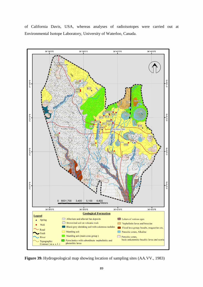
89
of California Davis, USA, whereas analyses of radioisotopes were carried out at
Environmental Isotope Laboratory, University of Waterloo, Canada.
Figure 39: Hydrogeological map showing location of sampling sites (AA.VV., 1983)

90
5.2.2 Laboratory analyses
(i) Stable isotopes (δ18
O and δ2H) measurement
imultaneous analysis of δ18
O and δ2H isotopes in groundwater samples were carried out at
Los Gatos Research, Inc., Mountain View, California, USA, using a Laser Water Isotope
Analyzer V2. Sample isotope ratios were standardized using a range of working standards
calibrated against Vienna Standard Mean Ocean Water (VSMOW) (Appendix 4). The
isotope values of hydrogen and oxygen are reported in δ-notation relative to VSMOW (Eq.
1). The δ-values are expressed as parts per thousand or permil (‰).The precision for
analyzed groundwater samples was ≤0.3‰ for δ 18
O and ≤0.8‰ for δ2H. The average and
standard deviation for an internal check dispersed throughout the run with known isotope
ratio values for the calibrated water is given in Table 18.
1000)1(std
sample
R
R (Eq. 1)
where Rsample is 18
O/16
O or 2H/
1H ratio of the water sample and Rstd is for the standard in
VSMOW.
Table 18: Mean and Standard deviation of water used for calibration
Measurable δ2H (‰) δ
18O (‰)
Known value -55.65 -8.04
Mean -54.59 -7.79
n 7.00 7.00
1 standard deviation (SD) 0.60 0.15
(ii) Radioisotopes measurement
Tritium was determined by the direct tritium method with a precision of ±8 TU using a
PerkinElmer LKB-WALLAC Quantulus 1220-002, USA (Appendix 5). The results are
expressed as tritium units (TU) whereby 1 TU = 3.221 picocuries/L or 1 TU = 0.11919
Becquerels/L.
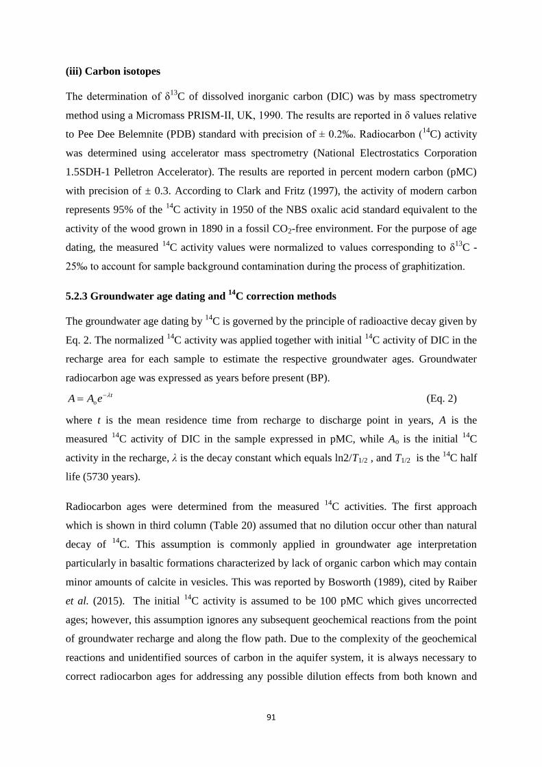
91
(iii) Carbon isotopes
The determination of δ13
C of dissolved inorganic carbon (DIC) was by mass spectrometry
method using a Micromass PRISM-II, K, 1990. The results are reported in δ values relative
to Pee Dee Belemnite (PDB) standard with precision of ± 0.2‰. Radiocarbon (14
C) activity
was determined using accelerator mass spectrometry (National Electrostatics Corporation
1.5SDH-1 Pelletron Accelerator). The results are reported in percent modern carbon (pMC)
with precision of ± 0.3. According to Clark and Fritz (1997), the activity of modern carbon
represents 95% of the 14
C activity in 1950 of the NBS oxalic acid standard equivalent to the
activity of the wood grown in 1890 in a fossil CO2-free environment. For the purpose of age
dating, the measured 14
C activity values were normalized to values corresponding to δ13
C -
25‰ to account for sample background contamination during the process of graphitization.
5.2.3 Groundwater age dating and 14
C correction methods
The groundwater age dating by 14
C is governed by the principle of radioactive decay given by
Eq. 2. The normalized 14
C activity was applied together with initial 14
C activity of DIC in the
recharge area for each sample to estimate the respective groundwater ages. Groundwater
radiocarbon age was expressed as years before present (BP).
teAA o (Eq. 2)
where t is the mean residence time from recharge to discharge point in years, A is the
measured 14
C activity of DIC in the sample expressed in pMC, while Ao is the initial 14
C
activity in the recharge, λ is the decay constant which equals ln2/T1/2 , and T1/2 is the 14
C half
life (5730 years).
Radiocarbon ages were determined from the measured 14
C activities. The first approach
which is shown in third column (Table 20) assumed that no dilution occur other than natural
decay of 14
C. This assumption is commonly applied in groundwater age interpretation
particularly in basaltic formations characterized by lack of organic carbon which may contain
minor amounts of calcite in vesicles. This was reported by Bosworth (1989), cited by Raiber
et al. (2015). The initial 14
C activity is assumed to be 100 pMC which gives uncorrected
ages; however, this assumption ignores any subsequent geochemical reactions from the point
of groundwater recharge and along the flow path. Due to the complexity of the geochemical
reactions and unidentified sources of carbon in the aquifer system, it is always necessary to
correct radiocarbon ages for addressing any possible dilution effects from both known and

92
uncertain sources (Clark & Fritz, 1997). There are several existing age correction techniques
applied in different environmental conditions depending on available data. This work applied
the statistical correction (Vogel, 1970) and δ13
C mixing method (Pearson & Hanshaw, 1970)
for 14C age correction. The δ
13C mixing method indirectly accounts for carbon chemistry in
terms of mixing of different components. Apart from mixing, the process includes an isotope
exchange process which is considered as a simple addition of one of the two components,
CO2 or solid carbonate, into the mixing (Fontes & Garnier, 1979). Fontes and Garnier (1979)
concluded that the Pearson method provides good approximation to the initial 14
C activity of
the total dissolved carbon with respect to their new approach. The initial activity of the total
dissolved carbon is estimated based on the 13
C content of each species (Clark & Fritz, 1997).
The correction factor (q) is given by:
carb
13
rech
13
carb
13
DIC
13
CδCδ
CδCδ
q
(Eq. 3)
where: δ13
CDIC = measured 13
C in groundwater
δ13
Crech = δ13
C value for DIC in the infiltrating groundwater
δ13
Ccarb = δ13
C of the calcite being dissolved
In this work, the values of δ13
Crech and δ13
Ccarb were opted to be -23‰ and 0‰ (Clark &
Fritz, 1997)
The statistical correction method as described by Vogel uses initial 14
C activity of 85% of the
modern carbon (Vogel, 1970). However, this approach gives ages which are probably too old
and does not account for the occurrence of recent waters in the recharge area (Fontes &
Garnier, 1979).
5.3 Results
5.3.1 Stable isotopes and tritium
Results of stable isotopes of hydrogen and oxygen (Table 19) plotted above and parallel to
both East African local meteoric water lines (LMWLs) and the global meteoric water line
(GMWL) (Fig. 40). The GMWL (δ2H = 8.13δ
18O + 10.8) is based on the refined Craig‘s line
(Clark & Fritz, 1997) whereas the LMWL for Dar es Salaam, Tanzania (δ2H = 7.01δ
18O +
6.83) and for Entebe, Uganda (δ2H = 7.38δ
18O + 10.78), are reported (Rozanski et al., 1996).
The best fit line for the analyzed stable isotopes is δ2H = 6.7δ
18O + 9.8. Water samples from
springs had δ2H values that ranged from -24.8 to -18.5‰ V MOW while samples of δ
18O
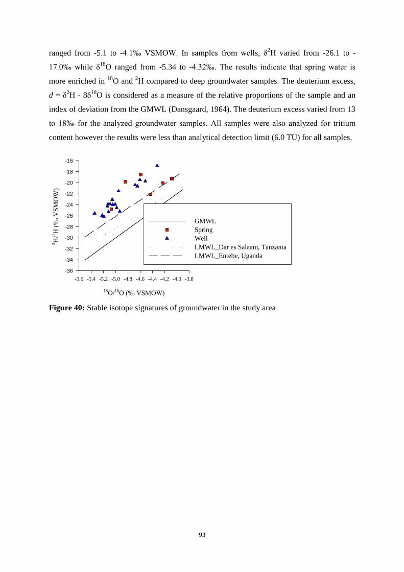
93
ranged from -5.1 to -4.1‰ V MOW. In samples from wells, δ2H varied from -26.1 to -
17.0‰ while δ18
O ranged from -5.34 to -4.32‰. The results indicate that spring water is
more enriched in 18
O and 2H compared to deep groundwater samples. The deuterium excess,
d = δ2H - 8δ
18O is considered as a measure of the relative proportions of the sample and an
index of deviation from the GMWL (Dansgaard, 1964). The deuterium excess varied from 13
to 18‰ for the analyzed groundwater samples. All samples were also analyzed for tritium
content however the results were less than analytical detection limit (6.0 TU) for all samples.
18O/16O (‰ VSMOW)
-5.6 -5.4 -5.2 -5.0 -4.8 -4.6 -4.4 -4.2 -4.0 -3.8
2H
/1H
(‰
VS
MO
W)
-36
-34
-32
-30
-28
-26
-24
-22
-20
-18
-16
GMWL
Spring
Well
LMWL_Dar es Salaam, Tanzania
LMWL_Entebe, Uganda
Figure 40: Stable isotope signatures of groundwater in the study area
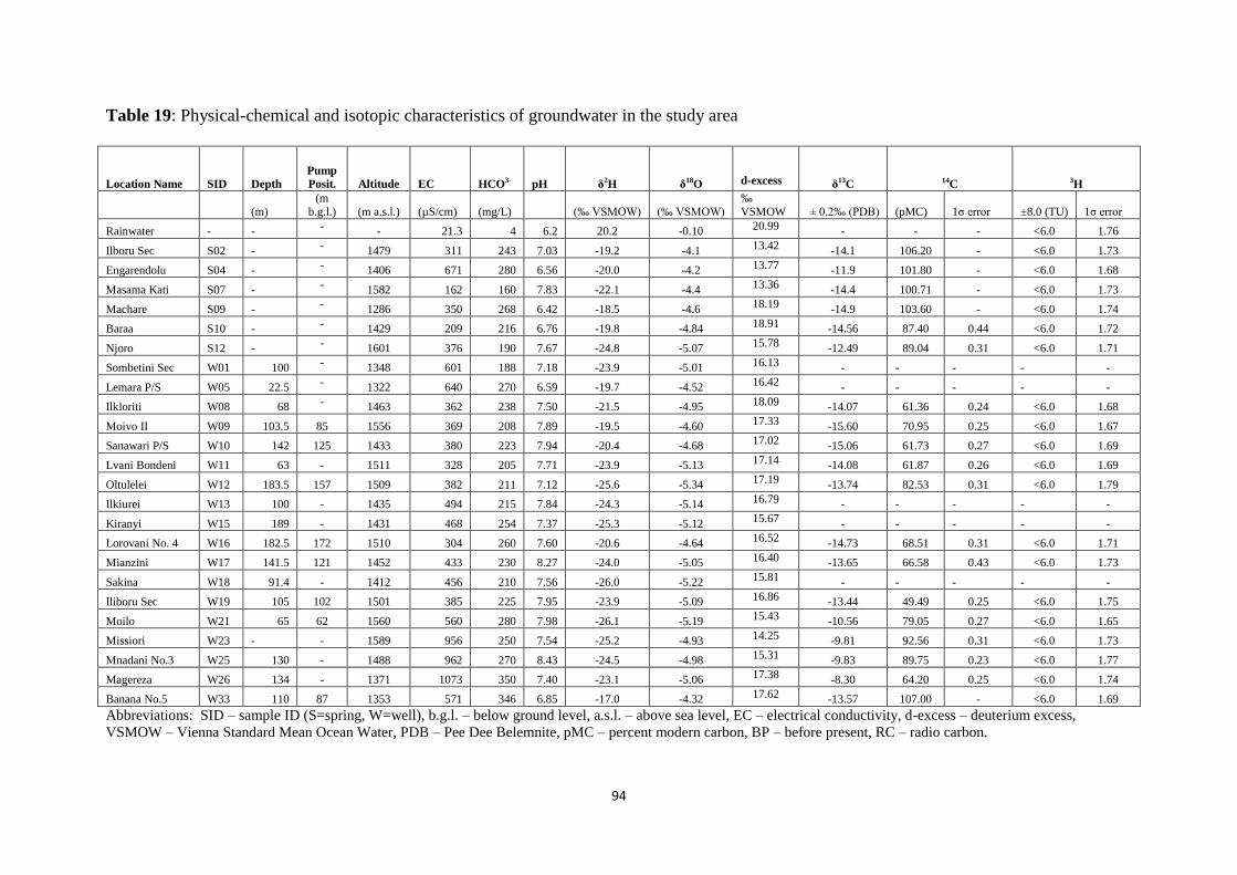
94
Table 19: Physical-chemical and isotopic characteristics of groundwater in the study area
Location Name SID Depth
Pump
Posit. Altitude EC HCO3- pH δ2H δ18O
d-excess δ13C 14C 3H
(m)
(m
b.g.l.) (m a.s.l.) (µS/cm) (mg/L) (‰ V MOW) (‰ V MOW)
‰
VSMOW ± 0.2‰ (PDB) (pMC) 1σ error ±8.0 (TU) 1σ error
Rainwater - - - - 21.3 4 6.2 20.2 -0.10 20.99 - - - <6.0 1.76
Ilboru Sec S02 - - 1479 311 243 7.03 -19.2 -4.1 13.42 -14.1 106.20 - <6.0 1.73
Engarendolu S04 - - 1406 671 280 6.56 -20.0 -4.2 13.77 -11.9 101.80 - <6.0 1.68
Masama Kati S07 - - 1582 162 160 7.83 -22.1 -4.4 13.36 -14.4 100.71 - <6.0 1.73
Machare S09 - - 1286 350 268 6.42 -18.5 -4.6 18.19 -14.9 103.60 - <6.0 1.74
Baraa S10 - - 1429 209 216 6.76 -19.8 -4.84 18.91 -14.56 87.40 0.44 <6.0 1.72
Njoro S12 - - 1601 376 190 7.67 -24.8 -5.07 15.78 -12.49 89.04 0.31 <6.0 1.71
Sombetini Sec W01 100 - 1348 601 188 7.18 -23.9 -5.01 16.13 - - - - -
Lemara P/S W05 22.5 - 1322 640 270 6.59 -19.7 -4.52 16.42 - - - - -
Ilkloriti W08 68 - 1463 362 238 7.50 -21.5 -4.95 18.09 -14.07 61.36 0.24 <6.0 1.68
Moivo II W09 103.5 85 1556 369 208 7.89 -19.5 -4.60 17.33 -15.60 70.95 0.25 <6.0 1.67
Sanawari P/S W10 142 125 1433 380 223 7.94 -20.4 -4.68 17.02 -15.06 61.73 0.27 <6.0 1.69
Lvani Bondeni W11 63 - 1511 328 205 7.71 -23.9 -5.13 17.14 -14.08 61.87 0.26 <6.0 1.69
Oltulelei W12 183.5 157 1509 382 211 7.12 -25.6 -5.34 17.19 -13.74 82.53 0.31 <6.0 1.79
Ilkiurei W13 100 - 1435 494 215 7.84 -24.3 -5.14 16.79 - - - - -
Kiranyi W15 189 - 1431 468 254 7.37 -25.3 -5.12 15.67 - - - - -
Lorovani No. 4 W16 182.5 172 1510 304 260 7.60 -20.6 -4.64 16.52 -14.73 68.51 0.31 <6.0 1.71
Mianzini W17 141.5 121 1452 433 230 8.27 -24.0 -5.05 16.40 -13.65 66.58 0.43 <6.0 1.73
Sakina W18 91.4 - 1412 456 210 7.56 -26.0 -5.22 15.81 - - - - -
Iliboru Sec W19 105 102 1501 385 225 7.95 -23.9 -5.09 16.86 -13.44 49.49 0.25 <6.0 1.75
Moilo W21 65 62 1560 560 280 7.98 -26.1 -5.19 15.43 -10.56 79.05 0.27 <6.0 1.65
Missiori W23 - - 1589 956 250 7.54 -25.2 -4.93 14.25 -9.81 92.56 0.31 <6.0 1.73
Mnadani No.3 W25 130 - 1488 962 270 8.43 -24.5 -4.98 15.31 -9.83 89.75 0.23 <6.0 1.77
Magereza W26 134 - 1371 1073 350 7.40 -23.1 -5.06 17.38 -8.30 64.20 0.25 <6.0 1.74
Banana No.5 W33 110 87 1353 571 346 6.85 -17.0 -4.32 17.62 -13.57 107.00 - <6.0 1.69
Abbreviations: SID – sample ID (S=spring, W=well), b.g.l. – below ground level, a.s.l. – above sea level, EC – electrical conductivity, d-excess – deuterium excess,
VSMOW – Vienna Standard Mean Ocean Water, PDB – Pee Dee Belemnite, pMC – percent modern carbon, BP – before present, RC – radio carbon.
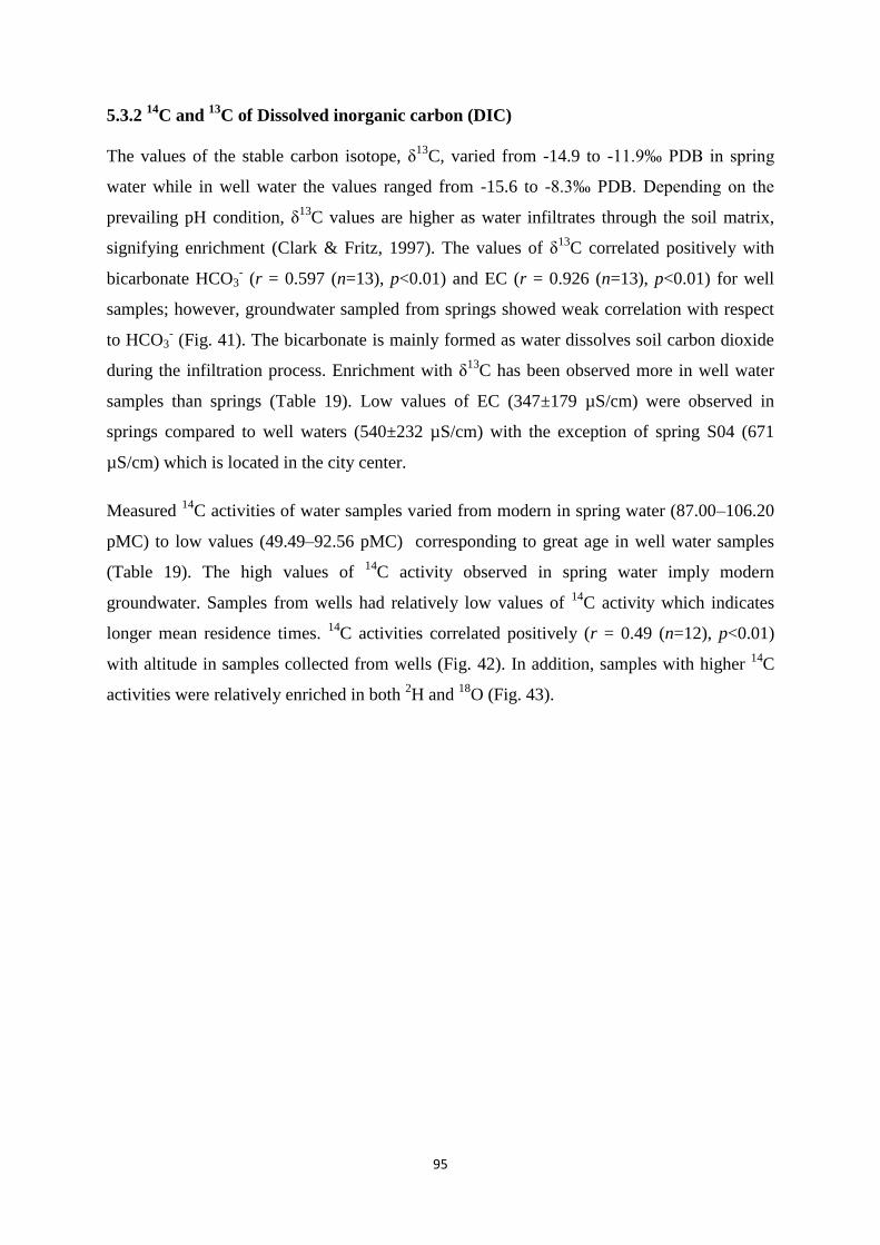
95
5.3.2 14
C and 13
C of Dissolved inorganic carbon (DIC)
The values of the stable carbon isotope, δ13
C, varied from -14.9 to -11.9‰ PDB in spring
water while in well water the values ranged from -15.6 to -8.3‰ PDB. Depending on the
prevailing pH condition, δ13
C values are higher as water infiltrates through the soil matrix,
signifying enrichment (Clark & Fritz, 1997). The values of δ13
C correlated positively with
bicarbonate HCO3- (r = 0.597 (n=13), p<0.01) and EC (r = 0.926 (n=13), p<0.01) for well
samples; however, groundwater sampled from springs showed weak correlation with respect
to HCO3- (Fig. 41). The bicarbonate is mainly formed as water dissolves soil carbon dioxide
during the infiltration process. Enrichment with δ13
C has been observed more in well water
samples than springs (Table 19). Low values of EC (347±179 µS/cm) were observed in
springs compared to well waters (540±232 µS/cm) with the exception of spring S04 (671
µS/cm) which is located in the city center.
Measured 14
C activities of water samples varied from modern in spring water (87.00–106.20
pMC) to low values (49.49–92.56 pMC) corresponding to great age in well water samples
(Table 19). The high values of 14
C activity observed in spring water imply modern
groundwater. Samples from wells had relatively low values of 14
C activity which indicates
longer mean residence times. 14
C activities correlated positively (r = 0.49 (n=12), p<0.01)
with altitude in samples collected from wells (Fig. 42). In addition, samples with higher 14
C
activities were relatively enriched in both 2H and
18O (Fig. 43).
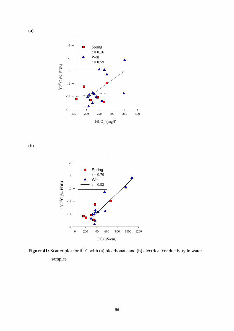
96
(a)
HCO3
- (mg/l)
150 200 250 300 350 400
13C
/12C
(‰
PD
B)
-16
-14
-12
-10
-8
-6Spring
r = 0.16
Well
r = 0.59
(b)
EC (µS/cm)
0 200 400 600 800 1000 1200
13C
/12C
(‰
PD
B)
-16
-14
-12
-10
-8
-6
Spring
r = 0.79
Well
r = 0.92
Figure 41: Scatter plot for δ13
C with (a) bicarbonate and (b) electrical conductivity in water
samples
97
5.3.3 Groundwater age
Radiocarbon dating revealed that groundwater in the study area was recharged in the
Quaternary period during late Holocene. The groundwater ages determined based on
corrected 14
C activity ranged from 1400 years BP to modern age. All spring water samples
fell under modern groundwater, however samples S10 and S12 were observed to have
relatively lower 14
C activities compared to others (Table 20). However, samples from wells
of different depths had groundwater ages ranging from 1400 to 100 years BP. The 14
C
activities (directly related to estimated groundwater ages) were positively correlated (r =
0.49) with altitude but no clear trends were observed with well depth (Fig. 42). Young
groundwater was observed in most wells located at high altitude and vice versa.
Table 20: Groundwater 14
C ages rounded to the nearest 102 years
Uncorrected age Corrected age
Location Name SID 14
C (pMC)
Vogel model (1970) Pearson model (1970)
Ilboru sec S02 106.2 Modern Modern Modern
Engarendolu S04 101.8 Modern Modern Modern
Masama kati S07 100.7 Modern Modern Modern
Machare S09 103.6 Modern Modern Modern
Baraa S10 87.4 1100 Modern Modern
Njoro S12 89.0 900 Modern Modern
Ilkloriti W08 61.4 4000 2700 300
Moivo II W09 70.9 2800 1500 Modern
Sanawari P/S W10 61.7 3900 2600 500
Lorovani bondeni W11 61.9 3900 2600 100
Oltulelei W12 82.5 1500 200 Modern
Lorovani No. 4 W16 68.5 3000 1800 Modern
Mianzini W17 66.6 3200 2000 Modern
Ilboru sec W19 49.5 5700 4500 1400
Moilo W21 79.0 1900 600 Modern
Missiori W23 92.6 600 Modern Modern
Mnadani No. 3 W25 89.7 900 Modern Modern
Magereza W26 64.2 3600 2300 Modern
Banana No. 5 W33 107.0 Modern Modern Modern
SID= Sample ID
98
(a)
Altitude (m a.s.l.)
1250 1300 1350 1400 1450 1500 1550 1600 1650
14C
act
ivit
y (
pM
C)
40
50
60
70
80
90
100
110
Spring
r = 0.23
Well
r = 0.49
(b)
Well depth (m)
40 60 80 100 120 140 160 180 200
14C
act
ivit
y (
pM
C)
40
50
60
70
80
90
100
110
Well
r = 0.13
Figure 42: Scatter plot for 14
C activity associated with (a) altitude and (b) well depth
(b)
99
5.4 Discussion
5.4.1 Moisture source
The stable isotope results gave a regression line with a slope of 6.7 which is close to but less
than the one established by Rozanski et al. 1993 for the GMWL, i.e., 8.13 (Fig. 40) (Clark &
Fritz, 1997) and the East African LMWL for Tanzania and Uganda with slope values of 7.01
and 7.38 respectively. Such a value indicates minimum or limited evaporation of infiltrated
rain water during the recharge period in the study area. These findings are also supported by
high deuterium excess values recorded by most groundwater samples ranging from 13 to
18‰ V MOW (Table 19). imilar results were reported in a study conducted by Ghiglieri et
al. (2012) at the North Eastern part of Mt. Meru where the values of deuterium excess varied
from 10 to 17‰ V MOW. Generally, at global scale the deuterium excess values range from
-2 to about 10–15‰ V MOW (Froehlich et al., 2001) depending on weather conditions.
Moreover, other work reported in the literature shows that warm and dry conditions enhance
evaporation, which leads to low or even negative deuterium excess values (Katsuyama et al.,
2011; Steen-Larsen et al., 2014; Katsuyama et al., 2015). High deuterium values observed in
the current study indicate dominance at low temperature and low humidity during
groundwater recharge (Plummer et al., 2012).
5.4.2 Groundwater recharge
High 14
C activities observed in spring water (98.1±7.9 pMC) correspond with recently
recharged groundwater in the study area (Fig. 43). The results indicate that the shallow
aquifer is actively recharged and responds to seasonal variations. This is supported by spring
flows (Fig. 44) whereby high flows are experienced during or immediate after the rainy
season and vice versa during dry conditions. The spatial distribution of 14
C activities shows
weak correlation (r = 0.49) with altitude (Fig. 42). The weak correlation may be due to
groundwater mixing from different layers probably recharged at different times. High 14
C
activity values were observed from wells located at high altitudes, the area which receives
more rainfall compared to low altitudes in the southern slopes of Mt. Meru. This suggests that
groundwater recharge is actively taking place in areas of high altitude on the slopes of the
Mountain. However, no clear trends were established between 14
C activity and well depth
(Fig. 42) probably indicating that most deep wells are tapping water from the same aquifer
but at different depth. Additionally, spring waters are relatively more enriched with respect to
hydrogen and oxygen isotopes (Table 19). This implies a higher fractionation effect due to
100
evaporation in shallow groundwater than in deep wells. However, the difference in stable
isotopic signatures is somehow narrow which implies that the recharge of both shallow and
deep groundwater took place under similar climatic conditions (Hoque & Burgess, 2012).
(a)
14C activity (pMC)
40 50 60 70 80 90 100 110
2H
/1H
(‰
VS
MO
W)
-28
-26
-24
-22
-20
-18
-16 Spring
Well
(b)
14C activity (pMC)
40 50 60 70 80 90 100 110
18O
/16O
(‰
VS
MO
W)
-5.6
-5.4
-5.2
-5.0
-4.8
-4.6
-4.4
-4.2
-4.0
Spring
Well
Figure 43: Relationship between stable isotopes and 14
C activity in water samples: (a)
hydrogen, and (b) oxygen isotopes. The wells inside the ellipse shape are
located in alluvial deposits.
Wells in
alluvial deposit
Wells in alluvial
deposit
(a)

101
Apart from 14
C dating, recent groundwater in springs was also evidenced by seasonal
variations of spring-flow data established for two springs (S04 and S07) from 2014 to 2016
(Fig. 44). The flows respond positively during rainy season by increasing significantly and
vice versa during dry months. This indicates that protection of these springs is of utmost
importance otherwise the recharge cycle will be interfered by rapid urbanization and
subsequently drying up or decrease of discharges. Nevertheless, the springs S10 and S12
recorded relatively lower values of 14
C activities, i.e., 87.4 and 89 pMC respectively. These
activities probably indicate that the two springs originate from deep aquifers which don‘t
respond easily to recharge from local precipitation.
Tritium results indicated low concentrations in all samples (<6.0 TU). However, the detection
limit (6 TU) of the method used was not able to delineate exactly the amount in each sample
which is expected to be low. In a similar study conducted on the northeastern Mt. Meru slope
(Ghiglieri et al., 2012), the maximum and mean values of 2.6 and 1.42 TU respectively were
recorded in groundwater samples. The study also indicated tritium content of 2.8 TU in a
rainwater sample. The low tritium content from both the previous and current studies suggest
that groundwater in the study area is recently recharged.
5.4.3 Groundwater exploitation
The estimated uncorrected groundwater 14
C ages for investigated wells ranged from 5700 to
about 600 years BP. Based on the Pearson corrected 14
C ages (Table 20), only four wells
(W08, W10, W11 and W19) revealed old groundwater (1400 to 100 years). In terms of
geological time scale, the ages seem to be young. However, it is quite a long period of time
for the case of continuous groundwater exploitation and its respective replenishment through
vertical recharge from local precipitation. The rest of the sampled wells have modern
groundwater which suggests that the aquifer is actively recharged. The persisting water-level
decline (Table 16) is probably a result of over-pumping practice as the groundwater
development is not adequately controlled in the study area. Nevertheless, groundwater ages
have been measured and reported worldwide ranging from months to millions of years
(Sturchio et al., 2004). Examples include (Bretzler et al., 2011) who reported groundwater
radiocarbon age in the main Ethiopian rift systems ranging from 800 to 5000 years BP at 80
to 260 m depths. In southern-east Tanzania (Bakari et al., 2012b) reported 14
C age of
groundwater was found to be ranging from 13 000 years BP in deep confined aquifers to
1300 years BP in shallow unconfined aquifers. Based on the current and previous studies,
102
most groundwaters in the Rift valley systems were recharged in late Pleistocene and
Holocene in the Quaternary period.
The age of groundwater is mainly affected by a number of factors including aquifer type and
geology of the area (Wassenaar et al., 1991; Sukhija et al., 1996; Bretzler et al., 2011). In the
current study young and modern groundwater (high 14
C activity values) were observed in
wells located at high altitude on the slopes of Mt. Meru which is the potential recharge zone
of the study area (Ong‘or & Long-cang, 2007). Other wells observed to have young water are
located in areas dominated by alluvial deposits in the northwest (Figs. 39 and 43). The oldest
groundwater (1400 years BP) was observed in a well located at low altitude (W19) in the
central part of the study area. This zone is mainly dominated by the basalts formation,
ranging from slightly weathered to fresh rocks (Appendix 2). Some of these wells are tapping
water from different geological layers because of well-screen positions (Appendix 2). The
position of screens at different depths within a single well could mean that the samples
collected represented mixed groundwater i.e., young and old waters together. The mixed
groundwater components could only be identified by applying a combination of tracers
suitable for dating young groundwater (less than 50 years) such as 3H/
3He or
85Kr (Mazor,
1993; Corcho Alvarado et al., 2007; ültenfuβ et al., 2011). The use of 14
C tracer facilitated
only identification of groundwater component with age greater than 100 years whereas other
components below this limit were categorized under modern groundwater. Generally, all
samples considered in this research represent groundwater recharged in late Holocene.
Decrease in water levels and subsequent decline in well yields in the research area have been
reported (Ong‘or & Long-cang, 2007). This is in line with estimated groundwater ages of up
to 1400 years BP. Such a long period of time is required to replenish the continuously
abstracted groundwater through production wells. Additionally, potential groundwater
recharge due to local precipitation is expected to be reduced because most production wells
are located within built-up residential areas and more development is still taking place,
expanding towards potential recharge areas. The development is likely to be interfering with
groundwater recharge rates, particularly the infiltration rate of precipitation (Rose & Peters,
2001; Han et al., 2017; Zomlot et al., 2017). Based on estimated 14
C ages, the aquifer storage
depletion in the study area is a result of groundwater over-pumping. However, future
investigation on other factors likely to affect recharge mechanisms need to be undertaken.
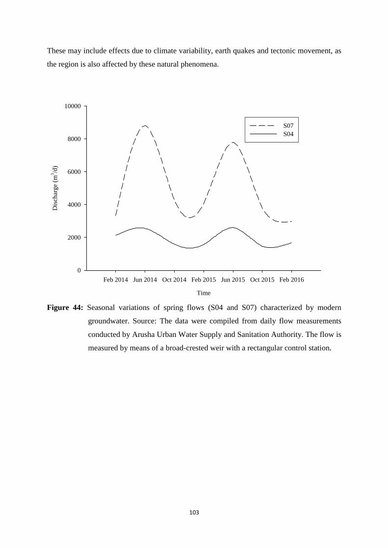
103
These may include effects due to climate variability, earth quakes and tectonic movement, as
the region is also affected by these natural phenomena.
Time
Feb 2014 Jun 2014 Oct 2014 Feb 2015 Jun 2015 Oct 2015 Feb 2016
Dis
char
ge
(m3/d
)
0
2000
4000
6000
8000
10000
S07
S04
Figure 44: Seasonal variations of spring flows (S04 and S07) characterized by modern
groundwater. Source: The data were compiled from daily flow measurements
conducted by Arusha Urban Water Supply and Sanitation Authority. The flow is
measured by means of a broad-crested weir with a rectangular control station.

104
5.5 Conclusions
The use of carbon-14 and stable isotope techniques for groundwater investigations has
revealed abstraction of relatively old groundwater from Arusha aquifers. Groundwater ages
estimated in the study area ranged from 1400 to 100 years BP. This long period of time is
required to replenish the continuously abstracted groundwater through production wells.
Generally, all groundwaters considered in this study were recharged in late Holocene.
However, no clear trends were established between 14
C activity and well depth, probably
indicating that most wells are tapping water from the same aquifer but at different depths or
layers depending on screen positions. The oldest groundwater (1400 years BP) was observed
in a well located at low altitude in the central part of the study area. This zone is mainly
dominated by basalts formation, ranging from slightly weathered to fresh rocks. The carbon-
14 results revealed young and modern groundwater in samples collected from shallow
aquifers i.e., spring water and wells located in areas dominated by alluvial deposits at high
altitudes. The presence of modern groundwater suggests that shallow aquifers are actively
recharged and respond positively to seasonal variations. Additionally, spring flow data
showed positive response during the rainy season by increasing flows significantly and vice
versa during dry months. This indicates that water sources including recharge zones in the
study area require a protection strategy to avoid drying up impact as well as decrease of
discharge. Potential groundwater recharge due to local precipitation is expected to be reduced
because most production wells and springs are located within built-up residential areas and
more development is still taking place, expanding towards the recharge areas. The
development is likely to be interfering with groundwater recharge mechanisms particularly
the infiltration rate of precipitation. Due to continuous pumping of groundwater for public
water supply in the study area and high mean residence times, as revealed by 14
C results, the
existing groundwater abstraction rate in the study area will not sustain the future demand.
However, future investigation on other factors likely to affect recharge rates needs to be
undertaken. These may include effects due climate variability, earth quakes and tectonic
movement, as the region is also affected by these natural phenomena.

105
CHAPTER SIX
GENERAL DISCUSSION, CONCLUSION AND RECOMMENDATIONS
6.1 General discussion
Groundwater development particularly when there is no adequate control can result into
adverse socioeconomic and ecological effects. The current global concern is groundwater
depletion due to increasing demand driven by intensive irrigated agriculture and rapid
population growth (Altchenko & Villholth, 2015; Amjath-Babu et al., 2016). Some of the
groundwater depletion effects include decreasing well yields, water level decline, rising
pumping costs, water quality deterioration and damaging of aquatic ecosystem (Konikow &
Kendy, 2005; Sishodia et al., 2017). In order to ensure aquifer sustainability proper planning
and management strategies should be developed and implemented. This needs adequate
knowledge of the respective aquifers in terms of groundwater quality and quantity as well as
recharge and discharge mechanisms. The quality of groundwater can be affected by either
natural or anthropogenic influences. All these factors are equally important and their
knowledge is vital in groundwater development and management. In many parts of Tanzania
the major concern of groundwater quality has been salinity and fluoride levels to the extent of
hindering various water sources from intended use. The findings of this study revealed among
other issues groundwater depletion, elevated fluoride levels (naturally occurring), and
abstraction of relatively old groundwater from Arusha wellfield.
Based on data from drilled boreholes and few published works, the level of groundwater
salinity varies across the country (Chapter 2, Fig. 2). The main determining factors of the
salinity occurrence and distributions include local geology, natural processes like tectonics
and volcanism as well as anthropogenic activities such as intensive irrigated agriculture and
fertilizer application. The coastal aquifers are characterized by brackish water (2271 to 5324
µS/cm) and saline groundwater in rare cases depending on the depth and distance of the well
from the shoreline. This indicates that seawater has laterally intruded and mixed with fresh
groundwater along the coastal region. Similar findings have been reported in previous works
and identified Na-Cl and NaCa-HCO3 as dominant water types (Mjemah, 2007; Bakari et al.,
2012a). However, confined deep coastal aquifers ranging from 200 to 600 m below ground
surface are reported to have relatively low level of conductivity, chloride and nitrate (Bakari
et al., 2012b).
106
The northern part of Tanzania which is the focus of this study together with central Rift
Valley were observed to have fresh groundwater but with relatively high salinity level (1000-
2000 µS/cm). The region is dominated by volcanic rocks in the north and crystalline
basement rocks in the central part which extends to Singida and Dodoma. Groundwater is
hosted in fractured and weathered formations dominated by relatively high salinity levels
(Nkotagu, 1996a; Bretzler et al., 2011; Ghiglieri et al., 2012) as a result of weathering and
mineral dissolution during water-rock interaction. This is also evidenced by high Na+ and low
Ca2+
ions in groundwater encountered in the region (Bretzler et al., 2011; Ghiglieri et al.,
2012) which implies long mean residence time. The levels of groundwater salinity in this
region extend to some areas of Lake Victoria region (Fig. 2). In some areas, high salinity
levels is reported to have been resulted from excessive irrigation water (Northey et al., 2006;
Batakanwa et al., 2013) though the effect is limited in shallow aquifers. In volcanic region
within the East African Rift System, trona dissolution is another factor which contribute to
high salinity levels in groundwater due to evaporation and leaching processes (Kaseva, 2006;
Pittalis, 2010). The rest of the country that is southern highlands, western and Lake Victoria
regions which lay between great lakes have fresh groundwater with conductivity less than
1000 µS/cm. Similarly, groundwater with conductivity ranging from 200 to 1200 µS/cm has
been encountered in central part of the country in particular Tabora region extending towards
Lake Victoria (Davies & Dochartaigh, 2002). The origin of groundwater salinity in this
region is due to dissolution of minerals from crystalline basement rocks which include
granites, gneisses, quartzite, and migmatites (Davies & Dochartaigh, 2002).
Fluoride concentration in the study area was generally high in both spring and well waters.
About eighty two (82) percent of the analyzed groundwater samples indicated fluoride
concentrations higher than WHO guidelines and Tanzanian drinking water standards (1.5
mg/l). The concentrations varied from one location to another indicating different mineralogy
or geological formation which may have different dissolution rate in the aquifer matrix
(Ghiglieri et al., 2012). In addition, water-rock interaction influences the concentration and
rate of fluoride release into groundwater system. Low fluoride concentration in fractured and
highly permeable phonolite hosted aquifers has been reported against high fluoride
concentration in water originating from basalt and lahars formation (Ghiglieri et al., 2010).
This suggests that variations of fluoride concentrations in groundwater are controlled by both
aquifer mineralogy and mean residence time. The spatial distribution analysis revealed high
fluoride concentration in northern and north-western parts of the study area compared to
107
south. High fluoride concentration in this zone is probably due to dominance in basalt
formation and other fluoride rich volcanic materials such as lahars and volcanic ash which are
known to contain and release significant amount of fluoride into groundwater in the region
(Ghiglieri et al., 2012).
The spatial analysis of hydrogeochemical characteristics of Arusha wellfield revealed Na-K-
HCO3 type of water. The chemical properties of groundwater are dominated by alkali
elements (Na+ and K
+) and weak acids (HCO3
-). Sodium ion was generally dominant in all
samples with Magnesium being the least cation in the study area (Na+ > Ca
2+ > K
+ > Mg
2+).
Such chemical behaviour in groundwater is explained by cations exchange reactions between
Na+ and Ca
2+ which occur as a result of water-rock interaction as water moves through
different mineralogical composition (Cerling et al., 1989; Ghiglieri et al., 2012; Utom et al.,
2013). High concentrations of dissolved ions such as Na+ and Ca
2+ were observed in deep
wells compared to shallow ones and springs. This suggests that groundwater abstracted from
deep aquifers has long mean residence time since the time of recharge. The
hydrogeochemistry of the groundwater is also supported with radioisotope signatures. The
results revealed high 14
C activities in spring water (98.1±7.9 pMC) corresponding with
recently recharged groundwater in the study area (chapter 5). The results indicate that the
shallow aquifer is actively recharged and responds to seasonal variations but deep aquifers
have relatively old water with mean radiocarbon age of up to 1400 years BP. The older
groundwater was observed in central part of the study area. The lithology of this area as
observed from well logs (Appendix 3) is dominated by basalts formation, ranging from
slightly weathered to fresh rocks. Recently recharged water was mostly encountered in
alluvial deposit formations believed to be the potential recharge area (Ong‘or & Long-cang,
2007). Another evidence of modern groundwater in the study area is tritium results which
indicated low concentrations in all samples. In a similar study conducted on the northeastern
Mt. Meru slope (Ghiglieri et al., 2012), the maximum and mean values of 2.6 and 1.42 TU
respectively were recorded in groundwater samples. The study also indicated tritium content
of 2.8 TU in a rainwater sample. The low tritium content from both the previous and current
studies suggest that groundwater in the study area is recently recharged. Nevertheless,
groundwater ages have been measured and reported worldwide ranging from months to
millions of years (Sturchio et al., 2004). In southern-east Tanzania, Bakari et al. (2012b)
reported relatively old 14
C age of groundwater ranging from 13 000 years BP in deep
confined aquifers to 1300 years BP in unconfined aquifers.
108
There is indication of groundwater contamination from anthropogenic influence particularly
in springs and shallow wells. This was evidenced by high nitrate levels exceeding the
recommended WHO guidelines (10.0 mg/l). The groundwater contamination in Tanzania is
contributed by on site sanitation practice such as use of pit latrine and septic tank system
connected to soak away pit (Nkotagu, 1996b; Mato & Kaseva, 1999; Kaown et al., 2009;
Elisante & Muzuka, 2015). However, very low concentrations of nitrate, chloride and
sulphate (Chapter 3) were observed in groundwater samples collected from deep wells
located in northern part of the study area. It was noted that shallow aquifers in the study area
have been affected by anthropogenic pollution though measures need to be taken for both
shallow and deep aquifers against such vulnerability.
A decrease in well discharge ranging from 10 to 57% for a period not exceeding 17 years has
been observed in different wells within the wellfield in the study area. The decrease in well
discharge is also accompanied by increasing drawdown of more than 1.0 m per year which
indicates a serious groundwater depletion problem in the study area. Similar impact has been
reported in central Tanzania (Taylor et al., 2013) and other many parts of the world which
exceeds 1.0 m per year in extreme development conditions such as China, Spain and United
States of America (Werner et al., 2013; Famiglietti, 2014; Huang et al., 2015; Custodio et al.,
2016; Kong et al., 2016). In this study, wells located in areas with less groundwater
development such as Lorovani and Ilboru (chapter 4, Figs. 21 and 26) indicated slightly
decrease in discharge compared to areas with intense groundwater development (Fig. 31).
Groundwater development effects have been reported in many parts of the world particularly
those with intense development. These impacts include land subsidence, deterioration of
groundwater dependent-ecosystem which include drying up of springs, wetlands and decrease
in volume of surface water bodies (Liu et al., 2011). Apart from groundwater depletion
effect, quality deterioration especially increasing fluoride concentrations in groundwater has
been reported. According to AUWSA personal communication (2015), one borehole at Ilboru
Secondary school was abandoned due to increase in fluoride level after pumping for a couple
of years. Therefore, an innovative approach is needed to rectify the ongoing unregulated
groundwater development in the Arusha wellfield. The legal and institution framework
responsible for water resources management are well structured. But the enforcement is still a
challenge partly due to inadequate human and financial resources (Kabote & John, 2017). It
was further revealed that lack of reliable hydrogeological information including interaction
109
between surface water and groundwater hinders water resources management efforts
particularly issuance of water use permit.
6.2 Conclusion
Geological and hydrogeochemical data, groundwater hydrographs, radioisotopes and
environmental stable isotopes techniques were use to assess the groundwater abstraction
trends and hydrogeochemical characteristics of Arusha wellfield in Arusha city. Groundwater
salinity in terms of conductivity (EC) was also used to delineate salinity occurrence and
distribution in different parts of Tanzania including Arusha where this study was carried out.
The hydrogeochemical investigation revealed Na-K-HCO3 water type with dominance of
Na+, K
+ and HCO3
- as major dissolved ions. The hydrogeochemical assessment results and
distribution of groundwater major cations (Na+ , Ca
2+ , K
+ , Mg
2+) and anions (HCO3
- , Cl
- ,
SO42-
, F-) in the study area indicate that groundwater chemistry is mainly influenced by
aquifer lithology than anthropogenic activities.
With exception of fluoride and faecal contamination (not covered in this work) the quality of
groundwater is generally suitable for drinking purpose and other socio-economic uses. About
eighty two (82) percent of the analyzed groundwater samples indicated fluoride
concentrations higher than WHO guidelines and Tanzanian drinking water standards (1.5
mg/l).
Groundwater hydrographs revealed groundwater depletion in the wellfield with a water level
decline of about 1.0 m per year. The decline is accompanied by reduction in well discharges
of about 10 to 57% observed from existing production wells for the past 17 years. The
decline in water levels and subsequent reduction in discharges is a result of over-abstraction
which is partly due to unregulated groundwater development in the area. More than 90% of
individual wells were drilled without groundwater permit from water resources management
authority. Therefore, even the amount of groundwater abstracted is not well known which
makes a great challenge and difficult in water resources management. It is also anticipated
that water level decline and subsequent reduction in well discharge will escalate the pumping
costs due to increased distance from the dynamic water level to the ground surface.
The use of 14
C and stable isotope techniques for groundwater investigations revealed
abstraction of relatively old groundwater from Arusha wellfield. Groundwater ages estimated
in the study area ranged from 1400 years BP to modern groundwater. Such a long period of
110
time is required to replenish the continuously abstracted groundwater through production
wells. However, high 14
C activities in spring water (98.1±7.9 pMC) signify recently
recharged groundwater in the study area. The presence of modern groundwater indicates that
shallow aquifers are actively recharged and respond positively to seasonal variations.
Groundwater salinity mapping revealed both brackish and freshwater in different parts of the
country. The brackish water is commonly found in coastal areas from Tanga in the north to
Lindi in southeast. The salinity levels of coastal groundwater in terms of average conductivity
ranged from 2271 to 5324 µS/cm. The elevated salinity level is mainly contributed by
seawater intrusion. However, it varies depending on the depth and distance of the well from
the shoreline. Confined deep coastal aquifers ranging from 100 to 600 m below ground
surface have been reported to have relatively low levels of conductivity, chloride and nitrate.
This suggests that the effect of seawater intrusion is more pronounced in unconfined shallow
aquifers which have undergone intensive groundwater development in most coastal areas of
Tanzania.
The northern and central Rift Valley region including Arusha was observed to have fresh
groundwater but with relatively high salinity level (1000-2000 µS/cm). The region falls
within the East African Rift System (EARS) which is dominated by volcanic and sedimentary
rocks. The high salinity levels are partly due to dissolution of trona (evaporate mineral)
which is commonly found in an EARS. The west part of the country including southern
highlands and Lake Victoria region observed to have fresh groundwater with salinity levels
less than 1000 µS/cm. The salinity level is relatively low and mainly influenced by local
geology and in some rare cases may be contributed by anthropogenic activities such as
irrigation water, fertilizer application and sewage effluents.
6.3 Recommendations
From the findings of this study, the following recommendations are put forward:
(i) The difference in fluoride concentration between spring and well waters is quite
significant and can be explained by geology of the area. This calls up on a detailed
geological study to precisely inform the entire spectrum of fluoride distribution and its
origin in the study area
111
(ii) It is recommended to carry out groundwater flow patterns modelling to show how
unregulated drilling affects the deep wells currently facing significant water level
decline and subsequently discharge reduction.
(iii) Pumping test is required in Arusha wellfield for the purpose of establishing the radius
of influence which can be used to guide the distance limit between wells for optimal
groundwater abstraction and proper management of the resource.
(iv) Groundwater balance of the wellfield could not be performed due to limited
information such as spring flow measurements in the area. Therefore, measurement of
spring and river flows including measurements of gain and loss of stream flow
between gauging stations is needed. Upon generation of the aforementioned
information, a comprehensive analysis and development of management strategy for
Arusha wellfield can be achieved.
(v) Over-abstraction has been revealed as one of the factors contributing to groundwater
depletion in the study area. Future investigation on other factors likely to affect
recharge mechanism needs to be undertaken.
(vi) Arusha wellfield is already stressed and it requires immediate interventions to ensure
adequate and reliable water supply for the City and its neighbourhoods. To meet the
current water demand which is already facing significant water deficit, consideration
of alternative water sources is inevitable. Among the possible alternatives could be
searching of new wellfield and rainwater harvesting.
(vii) More efforts to enforce existing laws and regulations governing water resources
management in the wellfield and at basin level are needed. This will aid in limiting
new development in depleted or stressed areas. Nevertheless, stringent measure
should be taken against individuals who unlawful conduct groundwater development.
(viii) Groundwater permit issuance: As proper planning and management of groundwater
resource depends on accurate information on which to base regulatory and
management decisions. The permit issuance should consider interconnection between
groundwater and surface water in the wellfield. Otherwise pumping water from
aquifers that are hydraulically connected with surface water may cause significant

112
effects such as reduced flows or drying up and subsequently damage of associated
ecosystems.
(ix) For the purpose of understanding the amount of groundwater abstracted from the
wellfield at a given time all production wells should have water flow meters and
boreholes which were unlawful drilled in the wellfield should be legalized and their
respective geological and hydrogeological data documented for proper water
resources management and environmental protection.

113
REFERENCES
AA.VV. 1983. Arusha Quarter Degree Sheet 55 scale 1:125 000. Geological Survey of
Tanzania.
Adelana, S. M. A. (2005). Nitrate health effects. Water Encyclopedia.
Aeschbach-Hertig, W., & Gleeson, T. (2012). Regional strategies for the accelerating global
problem of groundwater depletion. Nature Geoscience, 5(12): 853.
Ako, A. A., Shimada, J., Hosono, T., Ichiyanagi, K., Nkeng, G. E., Fantong, W. Y., … Roger,
N. N. (2011). Evaluation of groundwater quality and its suitability for drinking,
domestic, and agricultural uses in the Banana Plain (Mbanga, Njombe, Penja) of the
Cameroon Volcanic Line. Environmental Geochemistry and Health, 33(6): 559-575.
Alley, W. M., Reilly, T. E., & Franke, O. L. (1999). Sustainability of ground-water resources
vol 1186. US Department of the Interior, US Geological Survey, USA.
Altchenko, Y., & Villholth, K. (2015). Mapping irrigation potential from renewable
groundwater in Africa–a quantitative hydrological approach. Hydrology and Earth
System Sciences Discussions, 19(2): 1055-1067.
Amjath-Babu, T., Krupnik, T. J., Kaechele, H., Aravindakshan, S., & Sietz, D. (2016).
Transitioning to groundwater irrigated intensified agriculture in Sub-Saharan Africa:
An indicator based assessment. Agricultural Water Management, 168: 125-135.
Anderson, J., Baker, M., & Bede, J. (2012). Reducing emissions from deforestation and forest
degradation in the Yaeda Valley, Northern Tanzania Carbon Tanzania. 33pp.
Andrews, J. E., Riding, R., & Dennis, P. F. (1997). The stable isotope record of
environmental and climatic signals in modern terrestrial microbial carbonates from
Europe. Palaeogeography, Palaeoclimatology, Palaeoecology, 129(1-2): 171-189.
Apaydin, A. (2010). Relation of tectonic structure to groundwater flow in the Beypazari
region, NW Anatolia, Turkey. Hydrogeology Journal, 18(6): 1343-1356.
APHA (2012). Standard methods for the examination of water and wastewater. American
Public Health Association (APHA), American Water Works Association (AWWA),
Water Environmental Federation (WEF): Washington, DC, USA.

114
Arslan, S., Yazicigil, H., Stute, M., Schlosser, P., & Smethie, W. M. (2015). Analysis of
groundwater dynamics in the complex aquifer system of Kazan Trona, Turkey, using
environmental tracers and noble gases. Hydrogeology Journal, 23(1): 175-194.
AUWSA (2014). Medium Term Strategic plan (2015-2020). Arusha, Tanzania. 94pp.
Bakari, S. S., Aagaard, P., Vogt, R. D., Ruden, F., Johansen, I., & Vuai, S. A. (2012a).
Delineation of groundwater provenance in a coastal aquifer using statistical and
isotopic methods, Southeast Tanzania. Environmental earth Sciences, 66(3): 889-902.
Bakari, S. S., Aagaard, P., Vogt, R. D., Ruden, F., Brennwald, M. ., Johansen, I., …
Gulliksen, S. (2012b). Groundwater residence time and paleorecharge conditions in
the deep confined aquifers of the coastal watershed, South-East Tanzania. Journal of
Hydrology, 466:127-140.
Basalirwa, C., Odiyo, J., Mngodo, R., & Mpeta, E. (1999). The climatological regions of
Tanzania based on the rainfall characteristics. International Journal of Climatology,
19(1): 69-80.
Batakanwa, F., Mahoo, H., & Kahimba, F. (2013). Influence of irrigation water quality on
soil salinization in semi-arid areas: A case study of Makutopora, Dodoma-Tanzania.
Bretzler, A., Osenbrück, K., Gloaguen, R., Ruprecht, J. S., Kebede, S., & Stadler, S. (2011).
Groundwater origin and flow dynamics in active rift systems–A multi-isotope
approach in the Main Ethiopian Rift. Journal of Hydrology, 402(3): 274-289.
Brown, C., & Lall, U. (Ed.) (2006). Water and economic development: The role of variability
and a framework for resilience. In: Natural Resources Forum. Wiley Online Library,
pp. 306-317, 2006.
Bryan, K. (1919). Classification of springs. The Journal of Geology, 27(7): 522-561.
Carpenter, S. R., Fisher, S. G., Grimm, N. B., & Kitchell, J. F. (1992). Global change and
freshwater ecosystems. Annual Review of Ecology and Systematics, 23(1): 119-139.
Cerling, T. E., Pederson., B., & Von Damm, K. (1989). Sodium-calcium ion exchange in the
weathering of shales: Implications for global weathering budgets. Geology, 17(6):
552-554.
115
Chae, G. T., Yun, S. T., Mayer, B., Kim, K. H., Kim, S. Y., Kwon, J. S., … Koh, Y. K.
(2007). Fluorine geochemistry in bedrock groundwater of South Korea. Science of the
Total Environment, 385(1): 272-283.
Chaggu, E., Mashauri, D., Van Buuren, J., Sanders, W., & Lettinga, G. (2002). Excreta
disposal in Dar-es-Salaam. Environmental Management, 30(5): 0609-0620.
Chang, J., Wang, Y., Istanbulluoglu, E., Bai, T., Huang, Q., Yang, D., … Huang, S. (2015).
Impact of climate change and human activities on runoff in the Weihe River Basin,
China. Quaternary International, 380: 169-179.
Changming, L., Jingjie, Y., & Kendy, E. (2001). Groundwater exploitation and its impact on
the environment in the North China Plain. Water International, 26(2): 265-272.
Cheema, M. (2016). Agricultural production, water use and food availability in Pakistan:
Historical trends, and projections to 2050.
Chen, Z., Wei, W., Liu, J., Wang, Y., & Chen, J. (2011). Identifying the recharge sources and
age of groundwater in the Songnen Plain (Northeast China) using environmental
isotopes. Hydrogeology Journal, 19(1): 163-176.
Chenoweth, J. (2008). Minimum water requirement for social and economic development.
Desalination, 229(1): 245-256.
Clark, I. D., & Fritz, P. (1997). Environmental isotopes in hydrogeology CRC press.
Comte, J. C., Cassidy, R., Obando, J., Robins, N., Ibrahim, K., Melchioly, S., … Mohamed, I.
(2016). Challenges in groundwater resource management in coastal aquifers of East
Africa: Investigations and lessons learnt in the Comoros Islands, Kenya and Tanzania.
Journal of Hydrology: Regional Studies, 5: 179-199.
Corcho Alvarado, J. A., Purtschert, R., Barbecot, F., Chabault, C., Rueedi, J., Schneider, V.,
… Loosli, H. H. (2007). Constraining the age distribution of highly mixed
groundwater using 39
Ar: A multiple environmental tracer (3H/
3He,
85Kr,
39Ar, and
14C)
study in the semiconfined Fontainebleau Sands Aquifer (France). Water Resources
Research, 43, W03427.
116
Couth, R., & Trois, C. (2011). Waste management activities and carbon emissions in Africa.
Waste Management, 31(1): 131-137.
Currell, M. J., Han, D., Chen, Z., & Cartwright, I. (2012). Sustainability of groundwater
usage in northern China: dependence on palaeowaters and effects on water quality,
quantity and ecosystem health. Hydrological Processes, 26(26): 4050-4066.
Custodio, E. (2002). Aquifer overexploitation: what does it mean? Hydrogeology Journal,
10(2): 254-277.
Custodio, E., Andreu-Rodes, J. M., Aragón, R., Estrela, T., Ferrer, J., García-Aróstegui, J. L.,
… del Villar, A. (2016). Groundwater intensive use and mining in south-eastern
peninsular Spain: hydrogeological, economic and social aspects. Science of the Total
Environment, 559(302-316.
Davidson, I., & Ravi, S. (Ed.) (2005). Agglomerative hierarchical clustering with constraints:
Theoretical and empirical results. In: European Conference on Principles of Data
Mining and Knowledge Discovery Springer, pp. 59-70, 2005.
Davies, J., & Dochartaigh, B. (2002). Low permeability rocks in sub-Saharan Africa:
groundwater development in the Tabora Region, Tanzania.
Davis, G. H., Lee, C. K., Bradley, E., & Payne, B. (1970). Geohydrologic interpretations of a
volcanic island from environmental isotopes. Water Resources Research, 6(1): 99-
109.
Delinom, R. M. (2008). Groundwater management issues in the Greater Jakarta area,
Indonesia. TERC Bull, University of Tsukuba, 8(2): 40-54.
Dixon, B. (2005). Groundwater vulnerability mapping: a GIS and fuzzy rule based integrated
tool. Applied Geography, 25(4): 327-347.
Doell, P., Mueller Schmied, H., Schuh, C., Portmann, F. T., & Eicker, A. (2014).
Global‐scale assessment of groundwater depletion and related groundwater
abstractions: Combining hydrological modeling with information from well
observations and GRACE satellites. Water Resources Research, 50(7): 5698-5720.
117
Döll, P. (2009). Vulnerability to the impact of climate change on renewable groundwater
resources: a global-scale assessment. Environmental Research Letters, 4(3): 035006.
Douglas, A. A., Osiensky, J. L., & Keller, C. K. (2007). Carbon-14 dating of ground water in
the Palouse Basin of the Columbia River basalts. Journal of Hydrology, 334(3): 502-
512.
Drechsel, P., & Dongus, S. (2010). Dynamics and sustainability of urban agriculture:
examples from sub-Saharan Africa. Sustainability Science, 5(1): 69-78.
Elisante, E., & Muzuka, A. N. (2015). Occurrence of nitrate in Tanzanian groundwater
aquifers: A review. Applied Water Science, 7(1): 1-17.
Famiglietti, J. S. (2014). The global groundwater crisis. Nature Climate Change, 4(11): 945-
948.
Fan, A. M., & Steinberg, V. E. (1996). Health implications of nitrate and nitrite in drinking
water: an update on methemoglobinemia occurrence and reproductive and
developmental toxicity. Regulatory Toxicology and Pharmacology, 23(1): 35-43.
Fenta, A. A., Kifle, A., Gebreyohannes, T., & Hailu, G. (2015). Spatial analysis of
groundwater potential using remote sensing and GIS-based multi-criteria evaluation
in Raya Valley, Northern Ethiopia. Hydrogeology Journal, 23(1): 195-206.
Fitts, C. R. (2002). Groundwater science. Academic press.
Flint, A. L., Flint, L. E., Bodvarsson, G. S., Kwicklis, E. M., & Fabryka-Martin, J. (2001).
Evolution of the conceptual model of unsaturated zone hydrology at Yucca Mountain,
Nevada. Journal of Hydrology, 247: 1-30.
Fontes, J. C., & Garnier, J. M. (1979). Determination of the initial 14
C activity of the total
dissolved carbon: A review of the existing models and a new approach. Water
Resources Research, 15(2): 399-413.
Foster, S., & Chilton, P. (2003). Groundwater: the processes and global significance of
aquifer degradation. Philosophical Transactions of the Royal Society of London B:
Biological Sciences, 358: 1957-1972.
118
Franco, S., Gaetano, V., & Gianni, T. (2018). Urbanization and climate change impacts on
surface water quality: enhancing the resilience by reducing impervious surfaces.
Water Research, 144: 491-502.
Fritz, S. J. (1994). A survey of charge‐balance errors on published analyses of potable ground
and surface waters. Ground Water, 32(4): 539-546.
Froehlich, K., Gibson, J., & Aggarwal, P. (2001). Deuterium excess in precipitation and its
climatological significance. International Atomic Energy Agency, CandS Papers
Series, 13: 54-66.
Ghiglieri, G., Balia, R., Oggiano, G., & Pittalis, D. (2010). Prospecting for safe (low fluoride)
groundwater in the Eastern African Rift: the Arumeru District (Northern Tanzania).
Hydrology and Earth System Sciences Discussions, 14(6): 1081-1091.
Ghiglieri, G., Balia, R., Oggiano, G., Ardau, F., & Pittalis, D. (2008). Hydrogeological and
geophysical investigations for groundwater in the Arumeru District (Northern
Tanzania). Rendiconti Online SGI, 2(1): 431-432.
Ghiglieri, G., Pittalis, D., Cerri, G., & Oggiano, G. (2012). Hydrogeology and
hydrogeochemistry of an alkaline volcanic area: the NE Mt. Meru slope (East African
Rift–Northern Tanzania). Hydrology and Earth System Sciences, 16(2): 529-541.
Giordano, M. (2009). Global groundwater? Issues and solutions. Annual Review of
Environment and Resources, 34: 153-178.
GITEC & WEMA (2011). Groundwater Assessment of the Pangani Basin, Tanzania. The
Pangani Basin Water Board (PBWB) and the International Union for Conservation of
Nature (IUCN). 151pp.
Gizaw, B. (1996). The origin of high bicarbonate and fluoride concentrations in waters of the
Main Ethiopian Rift Valley, East African Rift system. Journal of African Earth
Sciences, 22(4): 391-402.
Gleeson, T., Alley, W. M., Allen, D. M., Sophocleous, M. A., Zhou, Y., Taniguchi, M. …
VanderSteen, J. (2012). Towards sustainable groundwater use: setting long‐term
goals, backcasting, and managing adaptively. Ground Water, 50(1): 19-26.
119
Gleeson, T., Befus, K. M., Jasechko, S., Luijendijk, E., & Cardenas, M. B. (2016). The global
volume and distribution of modern groundwater. Nature Geoscience, 9(2): 161-171.
Gleick, P. H. (1993). Water in crisis: a guide to the worlds fresh water resources.
Gorokhovich, Y. (2005). Abandonment of Minoan palaces on Crete in relation to the
earthquake induced changes in groundwater supply. Journal of Archaeological
Science, 32(2): 217-222.
Guo, H., Zhang, Y., Xing, L., & Jia, Y. (2012). Spatial variation in arsenic and fluoride
concentrations of shallow groundwater from the town of Shahai in the Hetao basin,
Inner Mongolia. Applied Geochemistry, 27(11): 2187-2196.
Hagedorn, B. (2015). Hydrochemical and 14C constraints on groundwater recharge and
interbasin flow in an arid watershed: Tule Desert, Nevada. Journal of Hydrology, 523:
297-308.
Hammer, Ø., Harper, D., & Ryan, P. (2001). Paleontological Statistics Software: Package for
Education and Data Analysis. Palaeontologia Electronica.
Han, D., Currell, M. J., Cao, G., & Hall, B. (2017). Alterations to groundwater recharge due
to anthropogenic landscape change. Journal of Hydrology, 554: 545-557.
Heathwaite, A. L. (2010). Multiple stressors on water availability at global to catchment
scales: understanding human impact on nutrient cycles to protect water quality and
water availability in the long term. Freshwater Biology, 55(suppl.1): 241-257.
Hellar-Kihampa, H., De Wael, K., Lugwisha, E., & Van Grieken, R. (2013). Water quality
assessment in the Pangani River basin, Tanzania: natural and anthropogenic
influences on the concentrations of nutrients and inorganic ions. International Journal
of River Basin Management, 11(1): 55-75.
Hoque, M. A., & Burgess, W. G. (2012). 14
C dating of deep groundwater in the Bengal
Aquifer System, Bangladesh: implications for aquifer anisotropy, recharge sources
and sustainability. Journal of Hydrology, 444: 209-220.
120
Huang, Z., Pan, Y., Gong, H., Yeh, P. J. F., Li, X., Zhou, D., … Zhao, W. (2015).
Subregional‐scale groundwater depletion detected by GRACE for both shallow and
deep aquifers in North China Plain. Geophysical Research Letters, 42(6): 1791-1799.
Ishaku, J., Ankidawa, B., & Abbo, A. (2015). Groundwater Quality and Hydrogeochemistry
of Toungo Area, Adamawa State, North Eastern Nigeria. American Journal of
Mining and Metallurgy, 3(3): 63-73.
Jenkins, M., Cumming, O., Scott, B., & Cairncross, . (2014). Beyond ‗improved‘towards
‗safe and sustainable‘urban sanitation: assessing the design, management and
functionality of sanitation in poor communities of Dar es Salaam, Tanzania. Journal
of Water Sanitation and Hygiene for Development, 4(1): 131-141.
Jha, M. K., Chowdhury, A., Chowdary, V., & Peiffer, S. (2007). Groundwater management
and development by integrated remote sensing and geographic information systems:
prospects and constraints. Water Resources Management, 21(2): 427-467.
Kabote, S. J., & John, P. (2017). Water governance in Tanzania: performance of governance
structures and institutions.
Kaihura, F., Stocking, M., & Kahembe, E. (2001). Soil management and agrodiversity: a case
study from Arumeru, Arusha, Tanzania. Proceedings of the Symposium on Managing
Biodiversity in Agricultural Systems, Montreal, Canada, 8 to 12 November, 2001.
Kaown, D., Koh, D. C., Mayer, B., & Lee, K. K. (2009). Identification of nitrate and sulfate
sources in groundwater using dual stable isotope approaches for an agricultural area
with different land use (Chuncheon, mid-eastern Korea). Agriculture, Ecosystems and
Environment, 132(3): 223-231.
Kaseva, M. (2006). Contribution of trona (magadi) into excessive fluorosis—a case study in
Maji ya Chai ward, northern Tanzania. Science of the Total Environment, 366(1): 92-
100.
Kashaigili, J. J. (2010). Assessment of groundwater availability and its current and potential
use and impacts in Tanzania. Report prepared for the International Water
Management Institute (IWMI), Colombo, Sri Lanka.
121
Katsuyama, M., Yoshioka, T., & Konohira, E. (2015). Spatial distribution of oxygen-18 and
deuterium in stream waters across the Japanese archipelago. Hydrology and Earth
System Sciences, 19: 1577-1588.
Katsuyama, M., Yoshioka, T., Konohira, E., Tayasu, I., & Tani, M. (2011). Spatial
distribution of oxygen-18 and deuterium in stream-and groundwaters across the
Japanese archipelago. AGU Fall Meeting Abstracts. 1114pp.
Kent, P. E. (1971). The geology and geophysics of coastal Tanzania. Institute of Geological
Sciences, Geophysical Papers, 6: 1-101.
Kijazi, A. L., & Reason, C. (2009). Analysis of the 2006 floods over northern Tanzania.
International Journal of Climatology, 29: 955-970.
Kitagawa, Y., Koizumi, N., Takahashi, M., Matsumoto, N., & Sato, T. (2006). Changes in
groundwater levels or pressures associated with the 2004 earthquake off the west
coast of northern Sumatra (M9. 0). Earth, Planets and Space, 58(2): 173-179.
Kløve, B., Ala-Aho, P., Bertrand, G., Gurdak, J. J., Kupfersberger, H., Kværner, J., … Rossi,
P. (2014). Climate change impacts on groundwater and dependent ecosystems.
Journal of Hydrology, 518(250-266.
Komakech, H. C., Van Der Zaag, P., & Van Koppen, B. (2012). The last will be first: Water
transfers from agriculture to cities in the Pangani river basin, Tanzania. Water
Alternatives, 5(3): 700.
Kong, X., Zhang, X., Lal, R., Zhang, F., Chen, X., Niu, Z., … Song, W. (2016). Groundwater
Depletion by Agricultural Intensification in China's HHH Plains, Since 1980s,
Advances in Agronomy. Elsevier, pp. 59-106.
Konikow, L. F., & Kendy, E. (2005). Groundwater depletion: A global problem.
Hydrogeology Journal, 13(1): 317-320.
Kump, L. R., Brantley, S. L., & Arthur, M. A. (2000). Chemical weathering, atmospheric
CO2, and climate. Annual Review of Earth and Planetary Sciences, 28(1): 611-667.
122
Laramee, J., & Davis, J. (2013). Economic and environmental impacts of domestic bio-
digesters: Evidence from Arusha, Tanzania. Energy for Sustainable Development,
17(3): 296-304.
Liu, J., Cao, G., & Zheng, C. (2011). Sustainability of groundwater resources in the North
China Plain, Sustaining groundwater resources. Springer, pp. 69-87.
Lu, Y., Song, S., Wang, R., Liu, Z., Meng, J., Sweetman, A. J., … Luo, W. (2015). Impacts
of soil and water pollution on food safety and health risks in China. Environment
International, 77: 5-15.
Malago, J., Makoba, E., & Muzuka, A. N. (2017). Fluoride Levels in Surface and
Groundwater in Africa: A Review. American Journal of Water Science and
Engineering, 3(1): 1-17.
Marchant, R., Richer, S., Capitani, C., Courtney-Mustaphi, C., Prendergast, M., Stump, D.,
… Vázquez, C. F. (2018). Drivers and trajectories of land cover change in East
Africa: Human and environmental interactions from 6000 years ago to present. Earth-
Science Reviews.
Mathouchanh, E., & Aeschbach-Hertig, W. (2015). Krypton separation from argon for Atom
Trap Trace Analysis of 85
Kr and 81
Kr.
Mato, R. R. A. M. (2002). Groundwater pollution in urban Dar es Salaam, Tanzania :
assessing vulnerability and protection priorities, Academic Award. Eindhoven
University of Technology. 215pp.
Mato, R. R. A. M., & Kaseva, M. (1999). Critical review of industrial and medical waste
practices in Dar es Salaam City. Resources, Conservation and Recycling, 25(3): 271-
287.
Mazor, E. (1993). Interrelations between groundwater dating, palaeoclimate and
palaeohydrology. Isotope Techniques in the Study of Past and Current Environmental
Changes in the Hydrosphere and the Atmosphere, IAEA-SM-329/65: 249-258.
Mbonile, M. J. (2005). Migration and intensification of water conflicts in the Pangani Basin,
Tanzania. Habitat International, 29(1): 41-67.
123
Miljević, N., & Golobočanin, D. (2007). Potential use of environmental isotopes in pollutant
migration studies. Archives of Industrial Hygiene and Toxicology, 58(2): 251-262.
Mjemah, I. (2007). Hydrogeological and hydrogeochemical investigation of a coastal aquifer
in Dar es Salaam, Tanzania. Academic Award, Department of Geology and soil
science Ghent University. 242pp.
Mooi, E., & Sarstedt, M. (2010). Cluster analysis.
Moturi, W. K., Tole, M. P., & Davies, T. C. (2002). The contribution of drinking water
towards dental fluorosis: a case study of Njoro Division, Nakuru District, Kenya.
Environmental Geochemistry and Health, 24(2): 123-130.
Mpanda, S. (1997). Geological development of the East African coastal basin of Tanzania,
Academic Award. Acta Universitatis Stockholmiensis.
Mtoni, Y., Mjemah, I. C., Bakundukize, C., Van Camp, M., Martens, K., & Walraevens, K.
(2013). Saltwater intrusion and nitrate pollution in the coastal aquifer of Dar es
Salaam, Tanzania. Environmental Earth Sciences, 70(3): 1091-1111.
Muhongo, S., Kapilima, S., & Mtoni, Y. (Ed.) (2000). Geological development and mineral
resources of the coastal basin of Tanzania. In: Proceedings of Workshops, 2000.
Muzuka, A. N., & Hillaire-Marcel, C. (1999). Burial rates of organic matter along the eastern
Canadian margin and stable isotope constraints on its origin and diagenetic evolution.
Marine Geology, 160(3): 251-270.
Muzuka, A. N. N., Dubi, A. M., Muhando, C. A., & Shaghude, Y. W. (2010). Impact of
hydrographic parameters and seasonal variation in sediment fluxes on coral status at
Chumbe and Bawe reefs, Zanzibar, Tanzania. Estuarine, Coastal and Shelf Science,
89: 137-144.
Muzuka, A. N. N., Ryner, M., & Holmgren, K. (2004). 12,000-Year, preliminary results of
the stable nitrogen and carbon isotope record from the Empakai Crater lake
sediments, Northern Tanzania. Journal of African Earth Sciences, 40(5): 293-303.
124
Naik, P. K., Tambe, J. A., Dehury, B. N., & Tiwari, A. N. (2008). Impact of urbanization on
the groundwater regime in a fast growing city in central India. Environmental
Monitoring and Assessment, 146(1): 339-373.
Nanyaro, J., Aswathanarayana, U., Mungure, J., & Lahermo, P. (1984). A geochemical model
for the abnormal fluoride concentrations in waters in parts of northern Tanzania.
Journal of African Earth Sciences, 2(2): 129-140.
United Republic of Tanzania (2013). Tanzania in Figures 2012. National Bureau of Statistics,
Ministry of Finance, Dar es Salaam, Tanzania. 81pp.
United Republic of Tanzania (2016). Tanzania Population Projection for Year 2016 and 2017
Based on 2012 Population and Housing Census. National Bureau of Statistics,
Ministry of Finance, Dar es Salaam, Tanzania.
Nigate, F., Ayenew, T., Belete, W., & Walraevens, K. (2017). Overview of the Hydrogeology
and Groundwater Occurrence in the Lake Tana Basin, Upper Blue Nile River Basin,
Social and Ecological System Dynamics. Springer, pp. 77-91.
Nkotagu, H. (1996a). The groundwater geochemistry in a semi-arid, fractured crystalline
basement area of Dodoma, Tanzania. Journal of African Earth Sciences, 23(4): 593-
605.
Nkotagu, H. (1996b). Origins of high nitrate in groundwater in Tanzania. Journal of African
Earth Sciences, 22(4): 471-478.
Nkotagu, H. H. (1989). Geochemistry of shallow groundwater at Kigamboni peninsula along
Dar es Salaam coastal strip Tanzania, Academic Award, pp. 739-748.
Noel, S., Soussan, J., & Barron, J. (2015). Water and Poverty Linkages In Africa: Tanzania
Case Study.
Northey, J., Christen, E., Ayars, J., & Jankowski, J. (2006). Occurrence and measurement of
salinity stratification in shallow groundwater in the Murrumbidgee Irrigation Area,
south-eastern Australia. Agricultural Water Management, 81(1-2): 23-40.
125
Öberg, H., Norström, E., Ryner, M. M., Holmgren, K., Westerberg, L. O., Risberg, J., …
Muzuka, A. N. N. (2013). Environmental variability in northern Tanzania from AD
1000 to 1800, as inferred from diatoms and pollen in Lake Duluti. Palaeogeography,
Palaeoclimatology, Palaeoecology, 374: 230-241.
Olaka, L. A., Odada, E. O., Trauth, M. H., & Olago, D. O. (2010). The sensitivity of East
African rift lakes to climate fluctuations. Journal of Paleolimnology, 44(2): 629-644.
Olobaniyi, S., & Owoyemi, F. (2006). Characterization by factor analysis of the chemical
facies of groundwater in the Deltaic plain sands Aquifer of Warri Western Niger
Delta, Nigeria. African Journal of Science and Technology Science and Engineering
Series, 7(1): 73-81.
Omambia, C. S., & Gu, Y. (2010). The cost of climate change in Tanzania: impacts and
adaptations. Journal of American Science, 6(3): 182-196.
Ong‘or, B. T., & Long-cang, S. (2007). Groundwater overdraft vulnerability and
environmental impact assessment in Arusha. Environmental Geology, 51(7): 1171-
1176.
Pearson, F., & Hanshaw, B. (1970). Sources of dissolved carbonate species in groundwater
and their effects on carbon-14 dating. Isotope hydrology. IAEA-SM-129/18: 271-285.
Piper, A. M. (1944). A graphic procedure in the geochemical interpretation of water‐analyses.
Eos, Transactions American Geophysical Union, 25(6): 914-928.
Pittalis, D. (2010). Interdisciplinary studies for the knowledge of the groundwater fluoride
contamination in the eastern African rift: Meru district-North Tanzania. Doctoral
dissertation, University of Sassari, Italy. 101pp.
Plummer, L. N., Eggleston, J. R., Andreasen, D., Raffensperger, J., Hunt, A., & Casile, G.
(2012). Old groundwater in parts of the upper Patapsco aquifer, Atlantic Coastal
Plain, Maryland, USA: evidence from radiocarbon, chlorine-36 and helium-4.
Hydrogeology Journal, 20(7): 1269-1294.

126
Rafique, T., Naseem, S., Usmani, T. H., Bashir, E., Khan, F. A., & Bhanger, M. I. (2009).
Geochemical factors controlling the occurrence of high fluoride groundwater in the
Nagar Parkar area, Sindh, Pakistan. Journal of Hazardous Materials, 171(1): 424-
430.
Rahmati, O., Samani, A. N., Mahdavi, M., Pourghasemi, H. R., & Zeinivand, H. (2015).
Groundwater potential mapping at Kurdistan region of Iran using analytic hierarchy
process and GIS. Arabian Journal of Geosciences, 8(9): 7059-7071.
Raiber, M., Webb, J., Cendón, D., White, P., & Jacobsen, G. (2015). Environmental isotopes
meet 3D geological modelling: conceptualising recharge and structurally-controlled
aquifer connectivity in the basalt plains of south-western Victoria, Australia. Journal
of Hydrology, 527(262-280.
Reddy, V. R. (2005). Costs of resource depletion externalities: a study of groundwater
overexploitation in Andhra Pradesh, India. Environment and Development
Economics, 10(4): 533-556.
Roberts, M. (2002). The Geochemical and Volcanological Evolution of the Mt. Meru Region,
Northern Tanzania, Academic Award. Cambridge, UK. 276pp.
Rose, S., & Peters, N. E. (2001). Effects of urbanization on streamflow in the Atlanta area
(Georgia, USA): a comparative hydrological approach. Hydrological Processes,
15(8): 1441-1457.
Rozanski, K., Araguas-Araguas, L., & Gonfiantini, R. (1996). Isotope patterns of
precipitation in the East African region. In: The limnology, climatology and
paleoclimatology of the East African Lakes: Edited by Thomas C. Johnson and Eric
O. Odada. Gordon and Breach. pp. 79-93.
Russo, T. A., & Lall, U. (2017). Depletion and response of deep groundwater to climate-
induced pumping variability. Nature Geoscience, 10(2): 105-111.
Rwebugisa, R. A. (Ed.) (2008). Groundwater Recharge Assessment in the Makutupora Basin,
Dodoma, Tanzania. Academic Award at International Institute for Geo-information
Science and Earth Observation. Enschede, The Netherlands. 111pp.
127
Sadashivaiah, C., Ramakrishnaiah, C., & Ranganna, G. (2008). Hydrochemical analysis and
evaluation of groundwater quality in Tumkur Taluk, Karnataka State, India.
International Journal of Environmental Research and Public Health, 5(3): 158-164.
Saxena, V., & Ahmed, S. (2001). Dissolution of fluoride in groundwater: a water-rock
interaction study. Environmental Geology, 40(9): 1084-1087.
Schlüter, T. (2008). Geological Atlas of Africa with Notes on Stratigraphy, Tectonics,
Economic Geology, Geohazards, Geosites, and Geoscientic Education on Each
Country (2nd
Edition). Springer-Verlag, Berlin. 308pp.
Schmoll, O., Howard, G., Chilton, J., & Chorus, I. (Eds.) (2006). Protecting groundwater for
health: managing the quality of drinking-water sources. IWA, London. 678pp.
Schwarzenbach, R. P., Egli, T., Hofstetter, T. B., Von Gunten, U., & Wehrli, B. (2010).
Global water pollution and human health. Annual Review of Environment and
Resources, 35(109-136.
Shiklomanov, I. A. (1998). World water resources A new appraisal and assessment for the
21st century.
Shindo, S. (1989). Study on the recharge mechanism and development of groundwater in the
inland area of Tanzania: Interim report of Japan-Tanzania Joint Research. 92pp.
Sigstedt, S. C., Phillips, F. M., & Ritchie, A. B. (2016). Groundwater flow in an
‗underfit‘carbonate aquifer in a semiarid climate: application of environmental tracers
to the Salt Basin, New Mexico (USA). Hydrogeology Journal, 24(4): 841-863.
Sishodia, R. P., Shukla, S., Graham, W. D., Wani, S. P., Jones, J. W., & Heaney, J. (2017).
Current and future groundwater withdrawals: Effects, management and energy policy
options for a semi-arid Indian watershed. Advances in Water Resources, 110: 459-
475.
Srinivas, Y., Hudson, O. D., Stanley, R. A., & Chandrasekar, N. (2014). Quality assessment
and hydrogeochemical characteristics of groundwater in Agastheeswaram taluk,
Kanyakumari district, Tamil Nadu, India. Chinese Journal of Geochemistry, 33(3):
221-235.

128
Srinivasamoorthy, K., Chidambaram, S., Prasanna, M., Vasanthavihar, M., Peter, J., &
Anandhan, P. (2008). Identification of major sources controlling groundwater
chemistry from a hard rock terrain—a case study from Mettur taluk, Salem district,
Tamil Nadu, India. Journal of Earth System Science, 117(1): 49-58.
Srinivasamoorthy, K., Vijayaraghavan, K., Vasanthavigar, M., Sarma, S., Chidambaram, S.,
Anandhan, P., … Manivannan, R. (2012). Assessment of groundwater quality with
special emphasis on fluoride contamination in crystalline bed rock aquifers of Mettur
region, Tamilnadu, India. Arabian Journal of Geosciences, 5(1): 83-94.
Steen-Larsen, H. C., Sveinbjörnsdottir, A. E., Peters, A. J., Masson-Delmotte, V., Guishard,
M. P., Hsiao, G., … White, J. W. C. (2014). Climatic controls on water vapor
deuterium excess in the marine boundary layer of the North Atlantic based on 500
days of in situ, continuous measurements. Atmospheric Chemistry and Physics, 14:
7741-7756.
Stewart, M. K. (2012). A 40-year record of carbon-14 and tritium in the Christchurch
groundwater system, New Zealand: Dating of young samples with carbon-14. Journal
of Hydrology, 430: 50-68.
Sturchio, N., Du, X., Purtschert, R., Lehmann, B., Sultan, M., Patterson, L., … Bailey, K.
(2004). One million year old groundwater in the Sahara revealed by krypton‐81 and
chlorine‐36. Geophysical Research Letters, 31(5).
Sukhija, B., Nagabhushanam, P., & Reddy, D. (1996). Groundwater recharge in semi-arid
regions of India: an overview of results obtained using tracers. Hydrogeology Journal,
4: 50-71
ültenfuβ, J., Purtschert, R., & Führböter, J. F. (2011). Age structure and recharge conditions
of a coastal aquifer (northern Germany) investigated with 39
Ar, 14
C, 3H, He isotopes
and Ne. Hydrogeology Journal, 19(1): 221-236.
Sundaram, B., Feitz, A., Caritat, P. D., Plazinska, A., Brodie, R., Coram, J., … Ransley, T.
(2009). Groundwater sampling and analysis–a field guide. Geoscience Australia,
Record, 27(95).
129
Tam, V. T., & Nga, T. T. V. (2018). Assessment of urbanization impact on groundwater
resources in Hanoi, Vietnam. Journal of Environmental Management, 227:107-116.
Tanzania Mereorological Agency (2013). Daily Weather Report (1955-2013). Arusha,
Tanzania.
Tanzania Standard (2016). Potable Water Specification-TZS 789:2016-EAS 12:2014. ICS:
67.060.20. Third Edition
Taylor, R. G., Todd, M. C., Kongola, L., Maurice, L., Nahozya, E., Sanga, H., …
MacDonald, A. M. (2013). Evidence of the dependence of groundwater resources on
extreme rainfall in East Africa. Nature Climate Change, 3(4): 374-385.
Tenge, A., De Graaff, J., & Hella, J. (2004). Social and economic factors affecting the
adoption of soil and water conservation in West Usambara highlands, Tanzania. Land
Degradation and Development, 15(2): 99-114.
Titus, R., Beekman, H., Adams, S., & Strachan, L. (2009). The basement aquifers of
Southern Africa. Water Research Commission Report No. TT: 428-09.
United Republic of Tanzania (1997). The National Environmental Policy.
United Republic of Tanzania (2002). The National Water Policy.
United Republic of Tanzania (2004). The Environmental Management Act.
United Republic of Tanzania (2009). Design Manual for Water Supply and Wastewater
Disposal. Third Edition. Ministry of Water and Irrigation, Tanzania.
United Republic of Tanzania (2009). The Water Resources and Management Act.
United Republic of Tanzania (2010). The Water Resources Management (Water Abstraction,
Use and Discharge) Regulations.
United Republic of Tanzania (2013). The Groundwater (Exploration and Drilling) Licensing
Regulations
130
Utom, A. U., Odoh, B. I., & Egboka, B. C. (2013). Assessment of hydrogeochemical
characteristics of groundwater quality in the vicinity of Okpara coal and Obwetti
fireclay mines, near Enugu town, Nigeria. Applied Water Science, 3(1): 271-283.
Van Camp, M., Mtoni, Y., Mjemah, I. C., Bakundukize, C., & Walraevens, K. (2014).
Investigating seawater intrusion due to groundwater pumping with schematic model
simulations: The example of the Dar es Salaam coastal aquifer in Tanzania. Journal of
African Earth Sciences, 96: 71-78.
Van Weert, F., Van der Gun, J., & Reckman, J. (2009). Global overview of saline
groundwater occurrence and genesis. International Groundwater Resources
Assessment Centre. Report No. GP 2009-1.
Venetsanou, P., Voudouris, K., Kazakis, N., & Mattas, C. (2015). Impacts of Urbanization,
Agriculture and Touristic Development on Groundwater Resources in the Eastern Part
of Thermaikos Gulf, North Greece. European Water, 51: 3-13.
Venkatramanan, S., Chung, S., Ramkumar, T., Gnanachandrasamy, G., Vasudevan, S., &
Lee, S. (2015). Application of GIS and hydrogeochemistry of groundwater pollution
status of Nagapattinam district of Tamil Nadu, India. Environmental Earth Sciences,
73(8): 4429-4442.
Vogel, J. (1970). Carbon-14 dating of groundwater. Isotope Hydrology, IAEA-SM-129/15:
225-240.
Wada, Y., van Beek, L. P., van Kempen, C. M., Reckman, J. W., Vasak, S., & Bierkens, M.
F. (2010). Global depletion of groundwater resources. Geophysical Research Letters,
37(20).
Wakode, H. B., Baier, K., Jha, R., & Azzam, R. (2018). Impact of urbanization on
groundwater recharge and urban water balance for the city of Hyderabad, India.
International Soil and Water Conservation Research, 6(1): 51-62.
Walraevens, K., Mjemah, I. C., Mtoni, Y., & Van Camp, M. (2015). Sources of salinity and
urban pollution in the Quaternary sand aquifers of Dar es Salaam, Tanzania. Journal
of African Earth Sciences, 102: 149-165.
131
Wassenaar, L., Aravena, R., & Fritz, P. (1991). Radiocarbon contents of dissolved organic
and inorganic carbon in shallow groundwater systems. Implications for groundwater
datingIsotope Techniques in Water Resources Development. IAEA-SM-319/5: 143-
151.
Werner, A. D., Zhang, Q., Xue, L., Smerdon, B. D., Li, X., Zhu, X., … Li, L. (2013). An
initial inventory and indexation of groundwater mega-depletion cases. Water
Resources Management, 27(2): 507-533.
Wilkinson, P., Mitchell, J., Cattermole, P., & Downie, C. (1986). Volcanic chronology of the
Men–Kilimanjaro region, Northern Tanzania. Journal of the Geological Society,
143(4): 601-605.
Wilson, J. L., & Guan, H. (2004). Mountain-Block Hydrology and Mountain-Front
Recharge. Groundwater Recharge in a Desert Environment: The Southwestern United
States, 113-137.
Wu, Q., Zhou, W., Wang, J., & Xie, S. (2009). Prediction of groundwater inrush into coal
mines from aquifers underlying the coal seams in China: application of vulnerability
index method to Zhangcun Coal Mine, China. Environmental Geology, 57(5): 1187-
1195.
Zipper, S. C., Soylu, M. E., Kucharik, C. J., & Loheide II, S. P. (2017). Quantifying indirect
groundwater-mediated effects of urbanization on agroecosystem productivity using
MODFLOW-AgroIBIS (MAGI), a complete critical zone model. Ecological
Modelling, 359: 201-219.
Zomlot, Z., Verbeiren, B., Huysmans, M., & Batelaan, O. (2017). Trajectory analysis of land
use and land cover maps to improve spatial–temporal patterns, and impact assessment
on groundwater recharge. Journal of Hydrology, 554: 558-569.
Zorita, E., & Tilya, F. F. (2002). Rainfall variability in Northern Tanzania in the March-May
season (long rains) and its links to large-scale climate forcing. Climate Research,
20(1): 31-40.
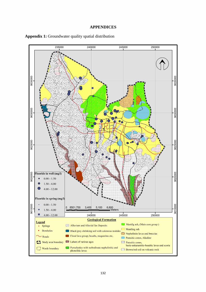
132
APPENDICES
Appendix 1: Groundwater quality spatial distribution

133

134
135
136
Appendix 2: Well lithology logs and completion details
Depth, m
Ø12"
0 G.L
8
16
24
32
40
48
56
64
72
80
88
96
104
112
120
128
136
144
152
160
168
176 P
183
W16
Depth, m
Ø12"
0 G.L
8
16
24
32
40
48
56
64
72
80
88
96
104
112
120
128
136
144
152
160 P
168
176
184
W12
Depth, m
Ø12"
0 G.L
8
16
24
32
40
48
56
64
72
80
88
96
P
104
108
W19
Key:
Clay
Weathered basalts
Fresh basalts
Volcanic sediments
Plain casing
Screens
Water level
P Pump location
Cement plug

137
Depth, m
Ø12"
0 G.L
8
16
24
32
40
48
56
64
72
80
88
96
104
112
120
P
128
136
140
142
W17
Depth, m
Ø12"
0 G.L
8
16
24
32
40
48
56
64
72
80
88
96
104
112
120
128 P
136
140
142
W10
Depth, m
Ø12"
0 G.L
8
16
24
32
40
48
56
64
72
80
P
88
96
104
108
W09
Key:
Clay
Weathered basalts
Fresh basalts
Volcanic sediments
Plain casing
Screens
Water level
P Pump location
Cement plug

138
Appendix 3: Well lithology logs
139
140
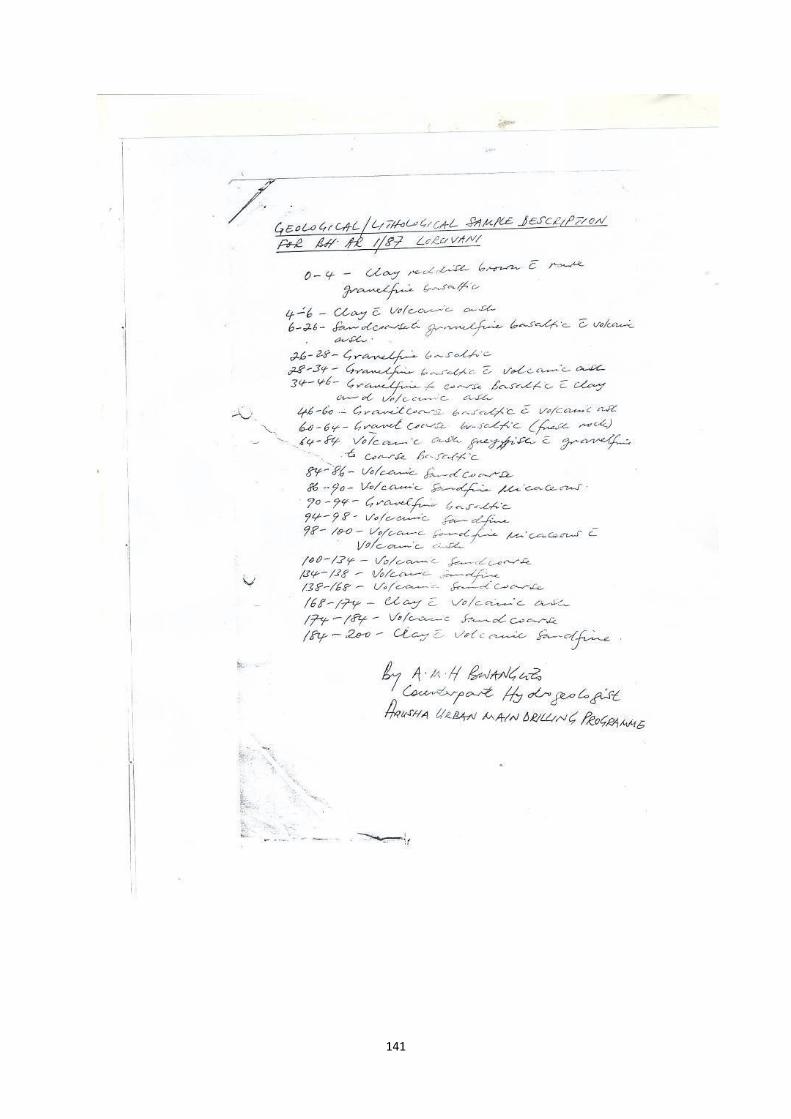
141
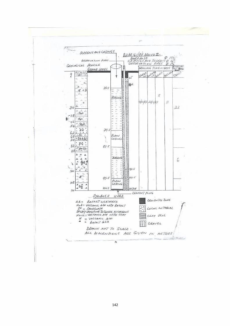
142

143
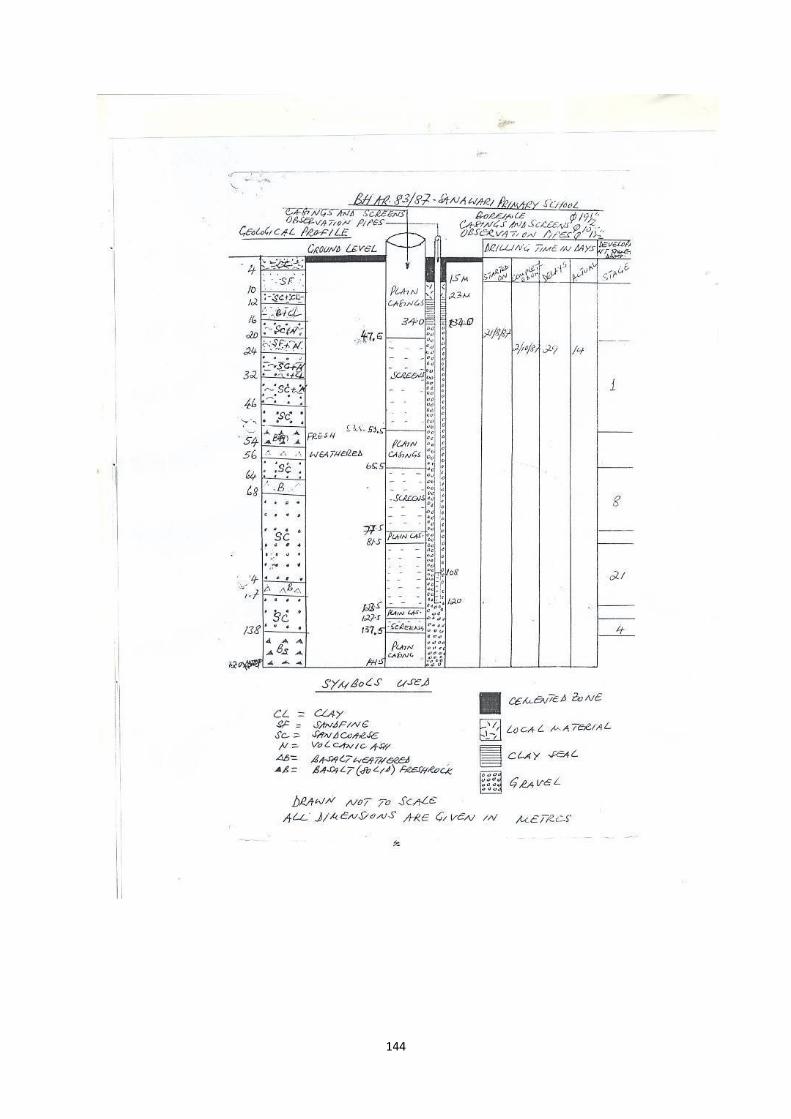
144

145
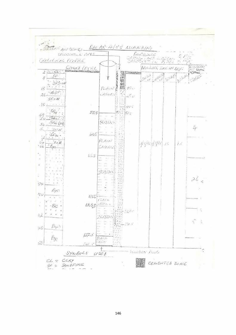
146

147
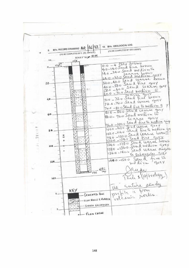
148
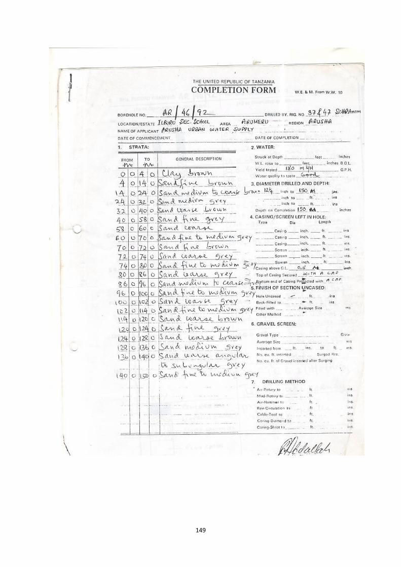
149
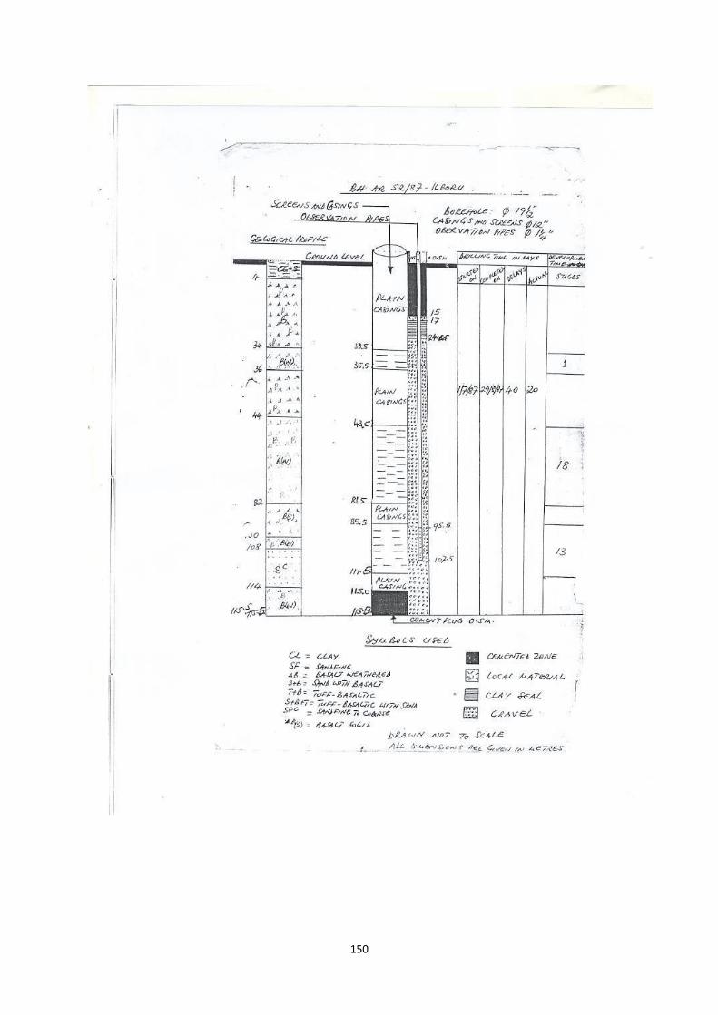
150
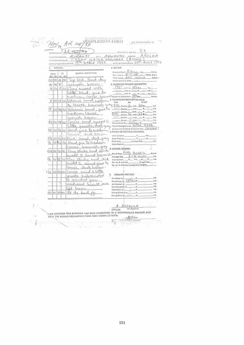
151
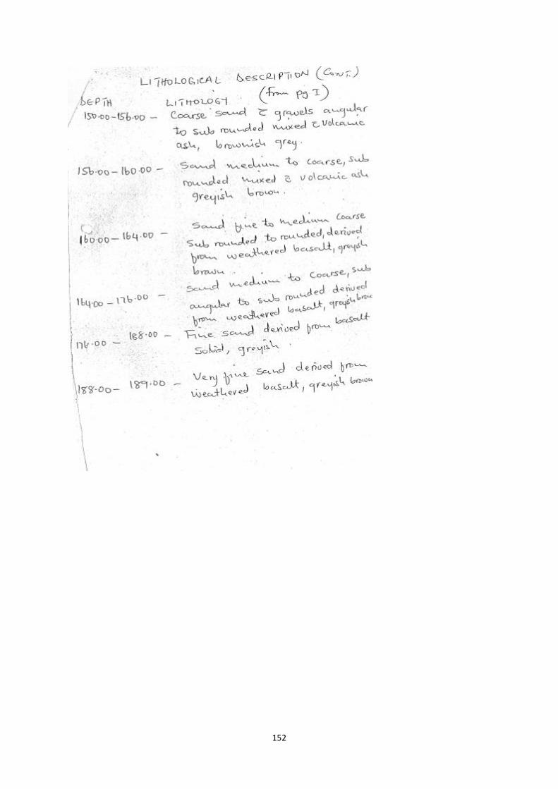
152

153
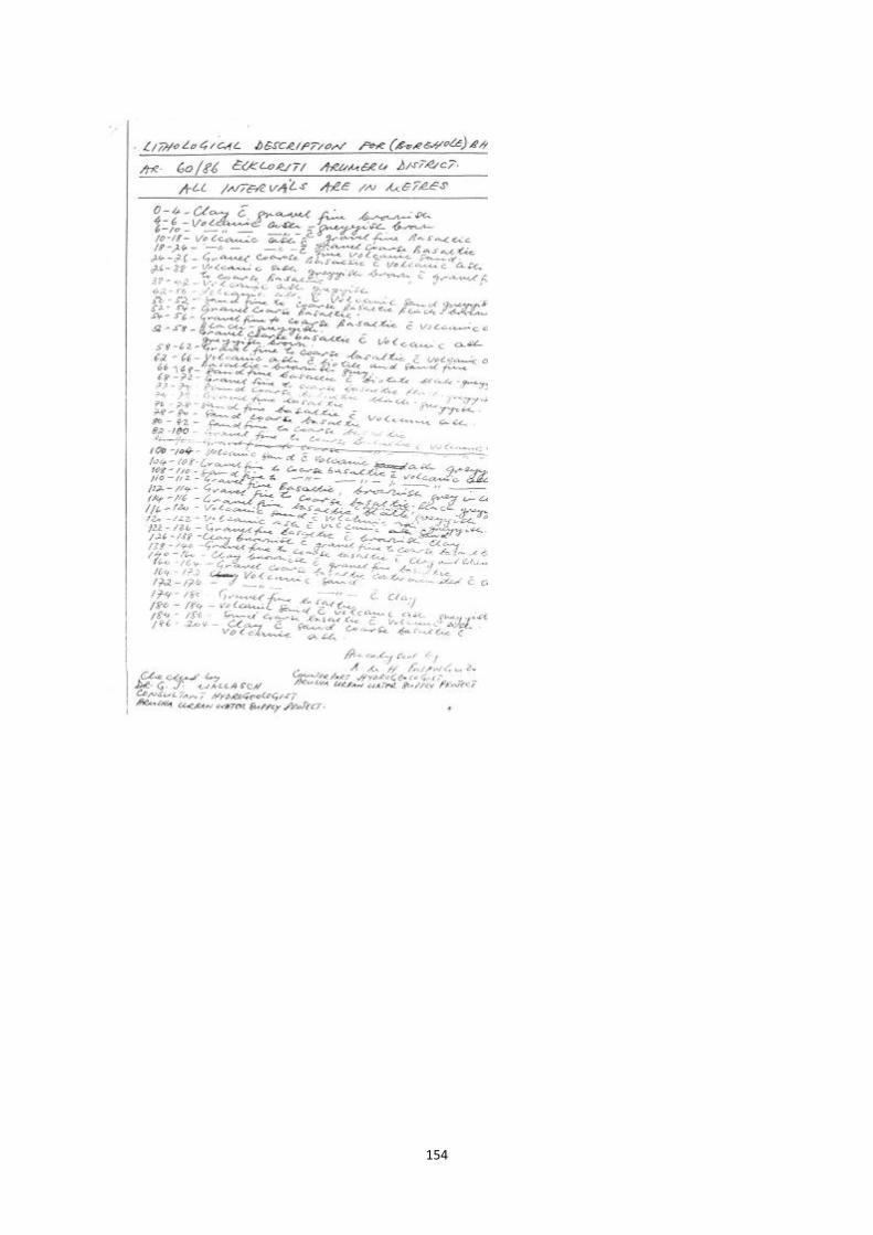
154

155
Appendix 4: Stable isotopes analysis procedure
Water Sample Preparation
The standard volume for water samples is 1-1.4 mL in a 2 mL GC vial. Contact the SIF about low volume samples.
Use vials with a write-on patch or use clear tape and permanent marker to label vials. Samples should be kept
refrigerated and in the dark for long-term storage. Use minimal headspace for shipping and storing water samples.
Additional preservation is not necessary. We do not accept samples preserved with mercuric chloride (HgCl2) or
poisoned with sodium azide (NaN3).
Supplies
Submit samples in standard autosampler vials (volume: 2 mL, 12 mm O.D. x 32 mm length) with wide-mouth 10-425
screw caps and double coated (PTFE/silicone/PTFE) septa. Samples not submitted in autosampler vials will be
charged a transfer fee
Organizing samples
For tracer studies, estimates on isotope values are required and samples must be organized by increasing enrichment.
Saline samples must be clearly marked with an estimate of the salinity. Organize saline samples in order of increasing
salinity. Units of ppt or mS/cm are preferred. Organize water samples in order of increasing conductivity.
Turbid water samples or water samples containing precipitate must be filtered prior to analysis. If SIF determines a
water sample requires filtering, a $5.00 fee will be charged per sample for this service.
The SIF only analyzes samples with a pH between 5 and 9. Samples outside this range must be neutralized prior to
shipment to the SIF.
Shipping
Carefully package racks of vials in ziplock bags, small boxes, or their original boxes. Then package these sets in a
larger sturdy box with styrofoam peanuts or bubble wrap. Make sure the samples are very secure; loose vials can
break during shipping. If samples must be shipped with a refrigerant, be sure to insulate your samples from freezing.
Avoid using dry ice as a refrigerant, as samples in direct contact with a refrigerant like dry ice will crack during
shipping. Coolers will not be returned.
Analysis of Water
The SIF provides simultaneous analysis of 18Oand D/H isotope ratios in liquid water samples using a Laser Water
Isotope Analyzer V2 (Los Gatos Research, Inc., Mountain View, CA, USA). For 18O and D/H at natural abundance,
each sample is injected at least six times. The average of the last four injections is used for isotope ratio calculations.
For enriched and saline samples, the number of injections is increased to ten. Sample isotope ratios are standardized
using a range of reference waters which have been calibrated against IAEA reference waters (VSMOW, GISP, and
SLAP). Precision for water samples at natural abundance is typically ≤0.3 per mil for 18O and ≤2.0 per mil for D/H.
Final 18O/16O and D/H values are reported relative to VSMOW.
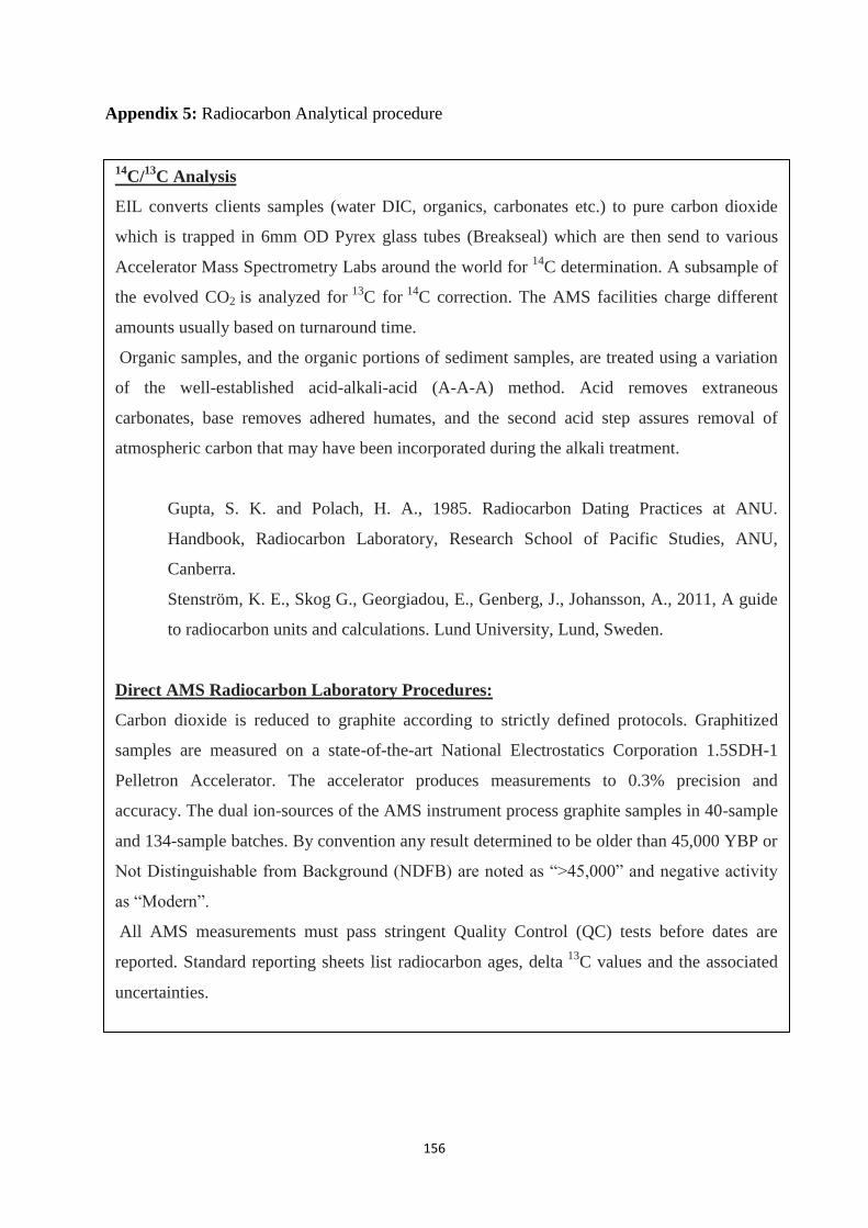
156
Appendix 5: Radiocarbon Analytical procedure
14C/
13C Analysis
EIL converts clients samples (water DIC, organics, carbonates etc.) to pure carbon dioxide
which is trapped in 6mm OD Pyrex glass tubes (Breakseal) which are then send to various
Accelerator Mass Spectrometry Labs around the world for 14
C determination. A subsample of
the evolved CO2 is analyzed for 13
C for 14
C correction. The AMS facilities charge different
amounts usually based on turnaround time.
Organic samples, and the organic portions of sediment samples, are treated using a variation
of the well-established acid-alkali-acid (A-A-A) method. Acid removes extraneous
carbonates, base removes adhered humates, and the second acid step assures removal of
atmospheric carbon that may have been incorporated during the alkali treatment.
Gupta, S. K. and Polach, H. A., 1985. Radiocarbon Dating Practices at ANU.
Handbook, Radiocarbon Laboratory, Research School of Pacific Studies, ANU,
Canberra.
Stenström, K. E., Skog G., Georgiadou, E., Genberg, J., Johansson, A., 2011, A guide
to radiocarbon units and calculations. Lund University, Lund, Sweden.
Direct AMS Radiocarbon Laboratory Procedures:
Carbon dioxide is reduced to graphite according to strictly defined protocols. Graphitized
samples are measured on a state-of-the-art National Electrostatics Corporation 1.5SDH-1
Pelletron Accelerator. The accelerator produces measurements to 0.3% precision and
accuracy. The dual ion-sources of the AMS instrument process graphite samples in 40-sample
and 134-sample batches. By convention any result determined to be older than 45,000 YBP or
Not Distinguishable from Background (NDFB) are noted as ―>45,000‖ and negative activity
as ―Modern‖.
All AMS measurements must pass stringent Quality Control (QC) tests before dates are
reported. Standard reporting sheets list radiocarbon ages, delta 13
C values and the associated
uncertainties.
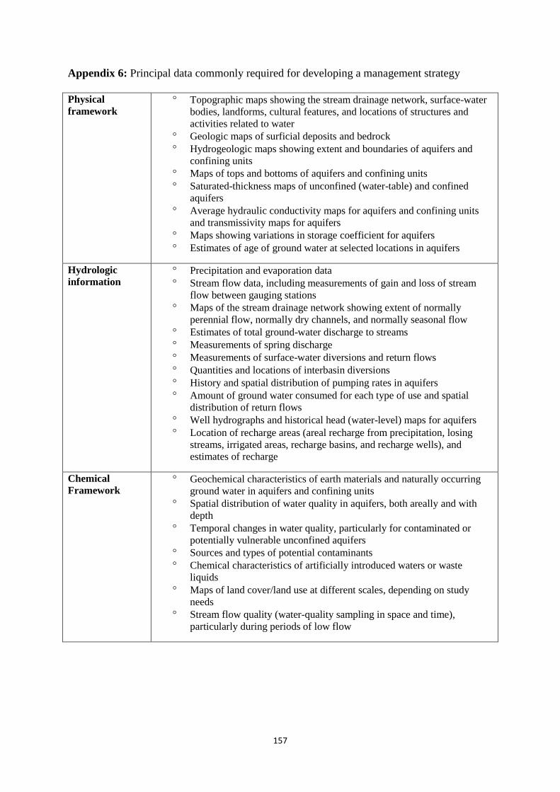
157
Appendix 6: Principal data commonly required for developing a management strategy
Physical
framework
Topographic maps showing the stream drainage network, surface-water
bodies, landforms, cultural features, and locations of structures and
activities related to water
Geologic maps of surficial deposits and bedrock
Hydrogeologic maps showing extent and boundaries of aquifers and
confining units
Maps of tops and bottoms of aquifers and confining units
Saturated-thickness maps of unconfined (water-table) and confined
aquifers
Average hydraulic conductivity maps for aquifers and confining units
and transmissivity maps for aquifers
Maps showing variations in storage coefficient for aquifers
Estimates of age of ground water at selected locations in aquifers
Hydrologic
information
Precipitation and evaporation data
Stream flow data, including measurements of gain and loss of stream
flow between gauging stations
Maps of the stream drainage network showing extent of normally
perennial flow, normally dry channels, and normally seasonal flow
Estimates of total ground-water discharge to streams
Measurements of spring discharge
Measurements of surface-water diversions and return flows
Quantities and locations of interbasin diversions
History and spatial distribution of pumping rates in aquifers
Amount of ground water consumed for each type of use and spatial
distribution of return flows
Well hydrographs and historical head (water-level) maps for aquifers
Location of recharge areas (areal recharge from precipitation, losing
streams, irrigated areas, recharge basins, and recharge wells), and
estimates of recharge
Chemical
Framework
Geochemical characteristics of earth materials and naturally occurring
ground water in aquifers and confining units
Spatial distribution of water quality in aquifers, both areally and with
depth
Temporal changes in water quality, particularly for contaminated or
potentially vulnerable unconfined aquifers
Sources and types of potential contaminants
Chemical characteristics of artificially introduced waters or waste
liquids
Maps of land cover/land use at different scales, depending on study
needs
Stream flow quality (water-quality sampling in space and time),
particularly during periods of low flow