Assessment of Future Climate and Vegetation Canopy Change ...envsys.co.kr/~envsys/paper/paper12/Assessment of... · length of 447 m and storage volume of 9.7 million m3. Details for

KSCE Journal of Civil Engineering (2014) 18(4):1185-1196

Copyright ⓒ2013 Korean Society of Civil Engineers

DOI 10.1007/s12205-013-0176-5

− 1185 −

pISSN 1226-7988, eISSN 1976-3808

www.springer.com/12205

Water Engineering

Assessment of Future Climate and Vegetation Canopy Change Impacts on

Hydrological Behavior of Chungju Dam Watershed using SWAT Model

Min Ji Park*, Rim Ha**, Nam Won Kim***, Kyoung Jae Lim****, and Seong Joon Kim*****

Received April 4, 2012/Revised 1st: September 21, 2012, 2nd: April 19, 2013/Accepted June 12, 2013/Published Online November 30, 2013

··································································································································································································································

Abstract

The impact on hydrological components including evapotranspiration, soil moisture content, groundwater recharge, and daminflow by the future potential climate and vegetation canopy changes was assessed for a dam watershed using Soil and WaterAssessment Tool (SWAT) model. The SWAT model was calibrated and verified using 9 years (1997-2006) and another 7 years(1990-1996) daily dam inflow data, respectively for a 6,585.1 km2 dam watershed located in the mountainous northeastern part ofSouth Korea. The second generation coupled global climate model (CGCM2) data of Canadian Centre for Climate modelling andanalysis (CCCma) from two Special Reports on Emissions Scenarios (SRES) climate change scenarios (A2 and B2) of theIntergovernmental Panel on Climate Change (IPCC) were adopted. The future vegetation canopy was developed by the nonlinearregression between monthly Leaf Area Index (LAI) from Terra MODIS (Moderate Resolution Imaging Spectroradiometer) imagesand monthly mean temperature of 7 years (2000-2006) data. The future prediction results with A2 and B2 scenarios showed that themaximum changes in annual dam inflow were predicted to be -18.2% in 2090s A2 scenario compared to 2000 baseline data. Thefuture seasonal maximum dam inflow changes appeared in fall period to be -31.0% for the A2 scenario. From the contributionanalysis of climate change and vegetation canopy for the overall future predicted results, the climate change primarily led the futureimpact on the predicted results. For the future vegetation impact on hydrological components, soil moisture was more sensitive thandam inflow and evapotranspiration.

Keywords: climate change, MODIS, LAI, SWAT, vegetation canopy, hydrological impact, dam inflow

··································································································································································································································

1. Introduction

Global changes of climate and atmosphere CO2 concentration

may have direct consequences on natural resources (Chaplot,

2007). Specifically,water is one of the vital natural resources that

are sensitive to climatic changes (IPCC, 1996; Gleick, 2000;

Water Resources Update, 2003). Future available water resource

can be evaluated by the hydrological impact studies using

outputs from the General Circulation Models (GCMs). GCMs

are commonly used for predicting climate change and for

providing inputs to hydrological models.

Many modeling studies deal with the impact of climate change

on river flows, however most of these studies are limited to the

application of present vegetation cover conditions. Vegetation

cover is the essential input data to hydrological models. Their

changes directly affect evapotranspiration, infiltration and soil

water storage which change the dynamics of surface runoff,

subsurface runoff and groundwater recharge. It is important to

consider the future vegetation cover. Future vegetation cover is

important for future behavior of hydrological components in

addition to climate changes.

The SWAT model (Arnold et al., 1998; Arnold and Fohrer,

2005) has proven to be an effective tool for assessing water

resource. SWAT has gained international acceptance as a robust

interdisciplinary watershed modeling tool as evidenced by

international SWAT conferences, hundreds of SWAT-related

papers presented at numerous other scientific meetings, and

dozens of articles published in peer-reviewed journals (Gassman

et al., 2007). Several SWAT studies provide useful insights

regarding the effects of arbitrary CO2 fertilization changes and

other climatic input shifts on plant growth, streamflow, and other

responses (Stonefelt et al., 2000, Fontaine et al., 2001, and Jha et

TECHNICAL NOTE

*Member, Environmental Researcher, Dept. of Civil and Environmental System Engineering, Konkuk University, Seoul 143-701, Korea; Water Quality

Control Center, National Institute of Environmental Research, Incheon 404-708, Korea (E-mail: [email protected])

**Member, Ph.D. Candidate, Dept. of Civil and Environmental System Engineering, Konkuk University, Seoul 143-701, Korea (E-mail: rim486@

konkuk.ac.kr)

***Member, Research Fellow, Korea Institute of Construction Technology, Ilsan 411-712, Korea (E-mail: [email protected])

****Professor, Dept. of Regional Infrastructure Engineering, Kangwon National University, Gangwon-do 200-701, Korea (E-mail: [email protected])

*****Member, Professor, Dept. of Civil and Environmental System Engineering, Konkuk University, Seoul 143-701, Korea (Corresponding Author, Email:

[email protected])

Min Ji Park, Rim Ha, Nam Won Kim, Kyoung Jae Lim, and Seong Joon Kim

− 1186 − KSCE Journal of Civil Engineering

al., 2006). Muttiah and Wurbs (2002), Gosain et al. (2006) and

Ryu et al. (2011) used SWAT to simulate the impacts of future

climate change scenario on the streamflows. Rosenberg et al.

(2003), Thomson et al. (2003), Rosenberg et al. (1999), Takle et

al. (2005), and Jha et al. (2004) predicted climate change impacts

on the hydrological components using GCMs, downscaling of

RCM (regional climate model). Eckhardt and Ulbrich (2003)

featured variable stomatal conductance and leaf area responses

by incorporating different stomatal conductance decline factors

and LAI values as a function of five main vegetation types.

The main goal of this study is to assess the potential impact of

climate changes on hydrological components of a watershed by

considering future vegetation cover conditions. The corresponding

future seasonal vegetation cover conditions were derived by the

MODIS LAI values estimated from the relationship of LAI-

Temperature nonlinear regression. The SWAT model was applied

to evaluate the future climate impact on hydrological components

using the climate change results of CCCma CGCM2 based on

SRES A2 and B2 for a 6,585.1 km2 mountainous watershed

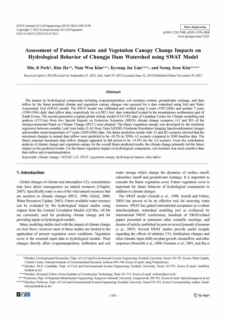
located in the upper east part of South Korea. Fig. 1 shows the

schematic diagram of this study.

2. Material and Method

2.1 Study Watershed

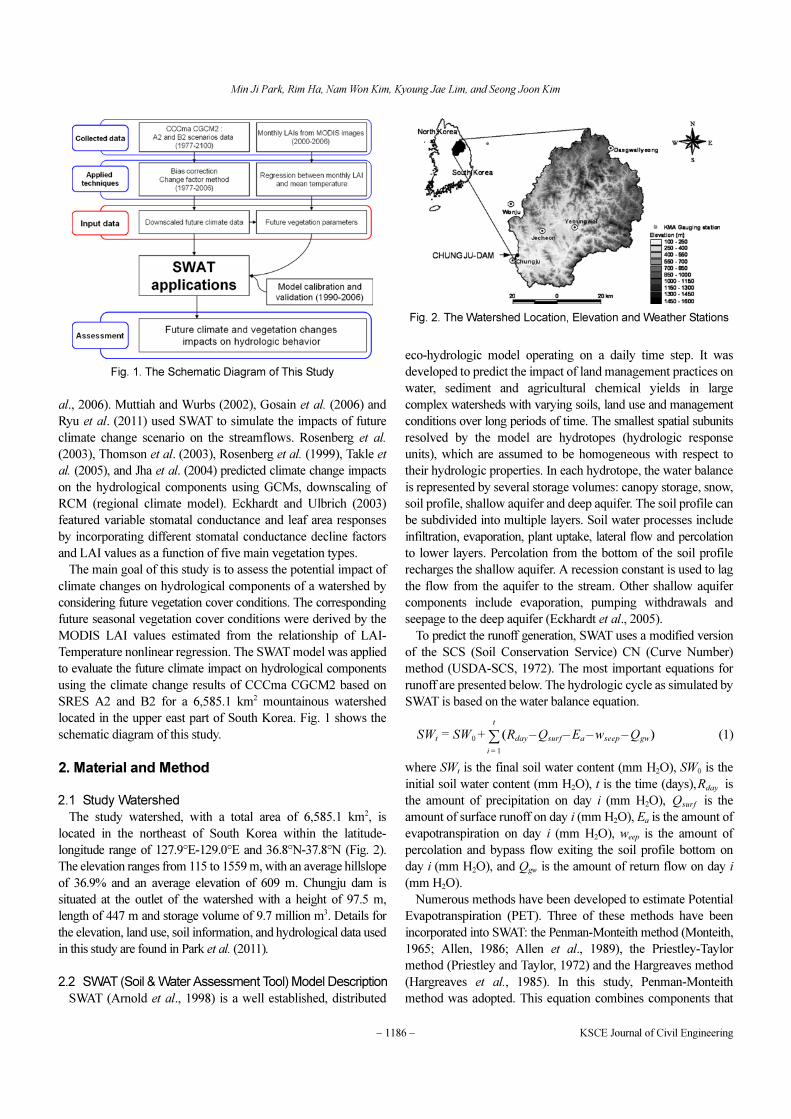
The study watershed, with a total area of 6,585.1 km2, is

located in the northeast of South Korea within the latitude-

longitude range of 127.9°E-129.0°E and 36.8°N-37.8°N (Fig. 2).

The elevation ranges from 115 to 1559 m, with an average hillslope

of 36.9% and an average elevation of 609 m. Chungju dam is

situated at the outlet of the watershed with a height of 97.5 m,

length of 447 m and storage volume of 9.7 million m3. Details for

the elevation, land use, soil information, and hydrological data used

in this study are found in Park et al. (2011).

2.2 SWAT (Soil & Water Assessment Tool) Model Description

SWAT (Arnold et al., 1998) is a well established, distributed

eco-hydrologic model operating on a daily time step. It was

developed to predict the impact of land management practices on

water, sediment and agricultural chemical yields in large

complex watersheds with varying soils, land use and management

conditions over long periods of time. The smallest spatial subunits

resolved by the model are hydrotopes (hydrologic response

units), which are assumed to be homogeneous with respect to

their hydrologic properties. In each hydrotope, the water balance

is represented by several storage volumes: canopy storage, snow,

soil profile, shallow aquifer and deep aquifer. The soil profile can

be subdivided into multiple layers. Soil water processes include

infiltration, evaporation, plant uptake, lateral flow and percolation

to lower layers. Percolation from the bottom of the soil profile

recharges the shallow aquifer. A recession constant is used to lag

the flow from the aquifer to the stream. Other shallow aquifer

components include evaporation, pumping withdrawals and

seepage to the deep aquifer (Eckhardt et al., 2005).

To predict the runoff generation, SWAT uses a modified version

of the SCS (Soil Conservation Service) CN (Curve Number)

method (USDA-SCS, 1972). The most important equations for

runoff are presented below. The hydrologic cycle as simulated by

SWAT is based on the water balance equation.

(1)

where SWt is the final soil water content (mm H2O), SW0 is the

initial soil water content (mm H2O), t is the time (days), is

the amount of precipitation on day i (mm H2O), is the

amount of surface runoff on day i (mm H2O), Ea is the amount of

evapotranspiration on day i (mm H2O), weep is the amount of

percolation and bypass flow exiting the soil profile bottom on

day i (mm H2O), and Qgw is the amount of return flow on day i

(mm H2O).

Numerous methods have been developed to estimate Potential

Evapotranspiration (PET). Three of these methods have been

incorporated into SWAT: the Penman-Monteith method (Monteith,

1965; Allen, 1986; Allen et al., 1989), the Priestley-Taylor

method (Priestley and Taylor, 1972) and the Hargreaves method

(Hargreaves et al., 1985). In this study, Penman-Monteith

method was adopted. This equation combines components that

SWt SW0 Rday Qsurf– Ea– wseep– Qgw–( )i 1=

t

∑+=

Rday

Qsurf

Fig. 1. The Schematic Diagram of This Study

Fig. 2. The Watershed Location, Elevation and Weather Stations

Assessment of Future Climate and Vegetation Canopy Change Impacts on Hydrological Behavior of Chungju Dam Watershed using SWAT Model

Vol. 18, No. 4 / May 2014 − 1187 −

account for energy needed to sustain evaporation, the strength of

the mechanism required to remove the water vapor and aerodynamic

and surface resistance terms. The Penman-Monteith equation is:

(2)

where λE is the latent heat flux density (MJ/m2·d), ∆ is the depth

rate evaporation (mm/d), is the slope of the saturation vapor

pressure-temperature curve, de/dT (kPa/oC), Hnet is the net radiation

(MJ/m2·d), is the heat flux density to the ground (MJ/m2·d),

is the air density (kg/m3), cp is the specific heat at constant

pressure (MJ/ kg·oC), is the saturation vapor pressure of air at

height z (kPa), ez is the water vapor pressure of air at height z

(kPa), γ is the psychrometric constant (kPa/oC), rc is the plant

canopy resistance (s/m), and ra is the diffusion resistance of the

air layer (aerodynamic resistance) (s/m).

Plant canopy resistance is estimated by dividing the minimum

surface resistance for a single leaf by one-half of the canopy LAI

(Jensen et al., 1990):

(3)

where rc is the canopy resistance (s/m), rl is the minimum effective

stomatal resistance of a single leaf (s/m), and LAI is the leaf area

index of the canopy.

2.3 The Spatial, Weather and Dam Inflow Data

The SWAT model requires data on elevation, land use, soil and

weather to assess the water yield at the desired locations of the

watershed. Elevation data were rasterized from a vector map of

1:5,000 scale that was supplied by the Korea National Geography

Institute. Based on the Digital Elevation Model, the watershed

was divided into 18 sub-basins. Soil data were rasterized from a

vector map of 1:50,000 scale that was supplied by the Korea

Rural Development Administration. The 2000 Landsat land use

data were obtained from the Water Management Information

System (http://www.wamis.go.kr/eng/main.aspx) operated by

Ministry of Land, Infrastructure and Transport. The monthly

MODIS Leaf Area Index was prepared for Penman-Monteith

evapotranspiration (ET). The dam inflow has been gauged since

1974 by the Korea Water Resources Corporation (K-water)

(Table 1).

Five weather stations closest to the watershed were selected as

seen in Fig. 2 and Table 2 summarizes the characteristics of

weather stations. The 30 years (1977-2006) daily maximum, and

minimum air temperatures (oC), daily precipitation (mm), relative

humidity (%), wind speed (m/sec), and solar radiation (MJ/m2)

were obtained from the Korea Meteorological Administration

(KMA).

2.4 The Future Climate Data

For future climate data, the CCCma CGCM2 data by two

SRES climate change scenarios (A2 and B2) of the IPCC were

adopted. The atmospheric component of the model is a spectral

model with triangular truncation at wave number 32 yielding a

surface grid resolution of roughly 3.7º by 3.7º and 10 vertical

levels (IPCC, 2006). Here, A2 is “high” GHG emission scenario

and B2 is “low” GHG emission scenario respectively.

In this study, a downscaling was performed by two steps.

Firstly, the GCM data was corrected to ensure that 30 years

observed data (1977-2006, baseline period) and GCM model

output of the same period have similar statistical properties by

the method used by Alcamo et al. (1997) and Droogers and Aerts

(2005) among the various statistical transformations. Details for

this method the results are found in Park et al. (2011).

Secondly, GCM model was downscaled using Change Factor

(CF) method (Diaz-nieto and Wilby, 2005; Wilby and Harris,

λE∆ Hnet G–( ) ρair cp ez

0ez–[ ] ra⁄⋅ ⋅+⋅

∆ γ 1 rc ra⁄+( )⋅+-------------------------------------------------------------------------------=

ρair

ez

0

rc rl 0.5 LAI⋅( )⁄=

Table 1. Data Sets for SWAT

Data Type Source Scale Data Description / Properties

Terrain Korea National Geography Institute 1/5,000 Digital Elevation Model (DEM)

Soil Korea Rural Development Administration 1/25,000Soil classifications and physical properties viz. texture, porosity,

field capacity, wilting point, saturated conductivity, and soil depth

Land Use Water Management Information System 30 m Landsat land use classification (2000 year, 9 classes)

Vegetation canopy Terra MODIS satellite image 1 km Leaf Area Index (LAI)

Weather Korea Meteorological Administration -Daily precipitation, minimum and maximum temperature, mean

wind speed and relative humidity data from 1977 to 2006

Streamflow Han River Flood Control Office - Daily dam inflow data from 1987 to 2006

Table 2. Weather Stations used for SWAT Simulation

NameData

periodsElevation

(m)Latitude Longitude

The average annual values

Precipitation(mm)

Temperature(oC)

Chungju 1977-2006 69.1 36-58-3.2 127-57-17.2 1,187.7 11.2

Daegwallyeong 1977-2006 842.5 37-41-2.9 128-45-39.6 1,717.2 6.4

Jecheon 1977-2006 263.2 37-9-23.3 128-11-46.6 1,295.0 10.1

Wonju 1977-2006 149.8 37-20-4.7 127-56-56 1,290.9 10.8

Yeoungwol 1995-2006 239.8 37-10-42.6 128-27-35.6 1,326.5 10.6



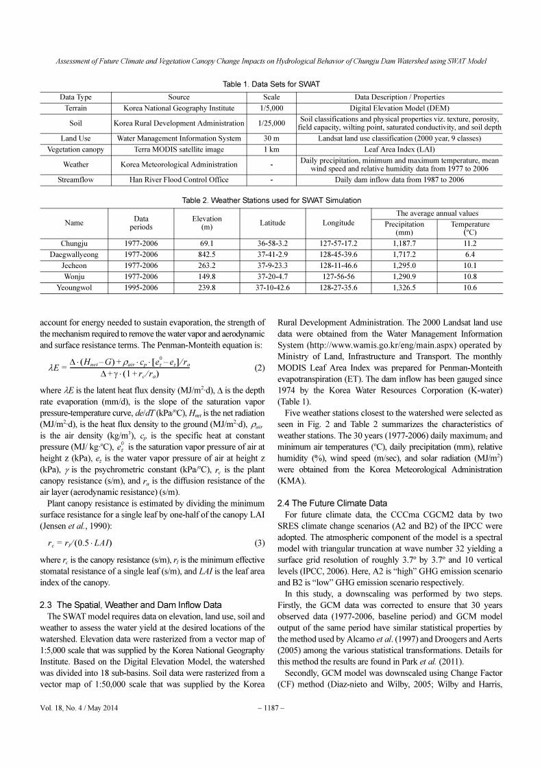
2006). Ahn et al. (2011) has a detailed description about this

process. The results are found in Fig. 3 for the future monthly

temperature and precipitation scenarios respectively. The results

showed that there are 5.5oC temperature and 45.5 mm precipitation

increase in case of A2 scenario, and 4.6oC temperature and 124.7

mm precipitation increase in case of B2 scenario for 2090

(Tables 3 and 4).

2.5 The Future Vegetation Data

To predict the future vegetation cover information, a nonlinear

regression between monthly LAI of each land cover from MODIS

satellite image and monthly mean temperature was accomplished.

The MODIS LAI 8-days composite scenes (MODI5A2, Collection

3) from 2000 to 2006 were downloaded from the Earth Observing

System Data Gateway (http://edcimswww.cr.usgs.gov/pub/

imswelcome/index.html), especially V003 (known as collection 3

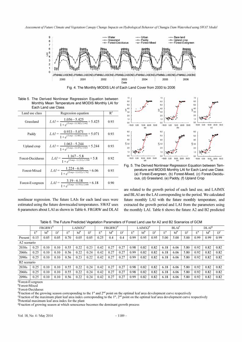
provisional data). Fig. 4 shows the monthly MODIS LAI of each

land cover from 2000 to 2006. Details for LAI the results are

found in Ha et al. (2010).

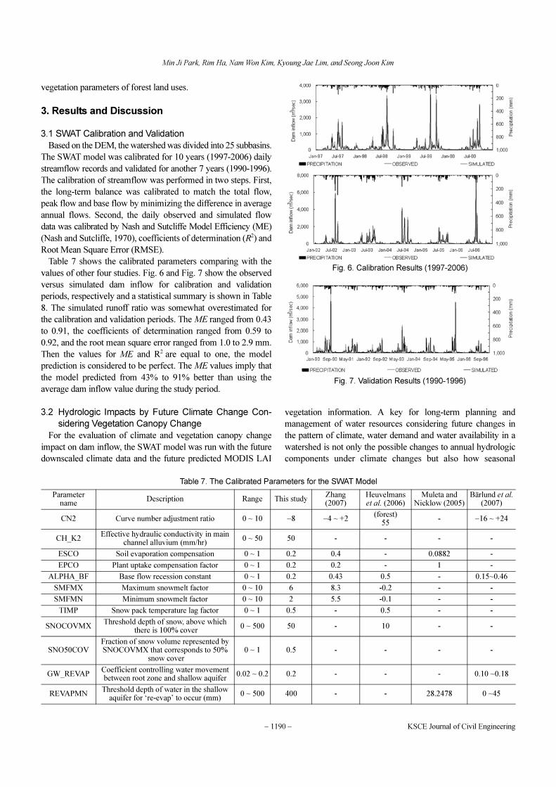
Table 5 and Fig. 5 show the nonlinear regression result using

seven years (2000-2006) monthly LAI and monthly mean

temperature from March to November. The monthly LAIs of

each land use from December to February could not be derived

because of snow cover, thus they were extrapolated using the

Fig. 3. The Future Adjusted and Downscaled Temperature and Precipitation Scenarios by CF Downscaling Method after Correcting the

GCM Data by 30-year Historical Data: (a) Precipitation (A2), (b) Precipitation (B2), (c) Temperature (A2), (d) Temperature (B2)

Table 3. The Changes (In Millimeter) in Seasonal Precipitation for the CF Method

Scenario2030s 2060s 2090s

A2 B2 A2 B2 A2 B2

Winter (December-February) +107.7 +132.7 +119.7 +119.7 +101.9 +84.6

Spring (March-May) +61.8 +73.6 +86.9 +86.9 +70.3 +96.8

Summer (June-August) -102.5 -107.9 -47.2 +135.2 -34.1 -46.6

Fall (September-November) -21.5 -14.8 -40.1 -40.1 -92.6 -10.1

Total +45.5 +83.5 +119.4 +301.8 +45.5 +124.7

Table 4. The Changes (In Degree) in Seasonal Temperature for the CF Method

Scenario2030s 2060s 2090s

A2 B2 A2 B2 A2 B2

Winter (December-February) +4.8 +5.2 +4.7 +4.7 +5.8 +5.8

Spring (March-May) -1.9 -1.9 -1.4 -1.4 +0.5 -0.6

Summer (June-August) +3.8 +3.5 +4.0 +4.0 +6.1 +4.8

Fall (September-November) +7.3 +7.6 +8.2 +8.2 +9.5 +8.3

Average +3.5 +3.6 +3.9 +3.9 +5.5 +4.6


Vol. 18, No. 4 / May 2014 − 1189 −

Fig. 4. The Monthly MODIS LAI of Each Land Cover from 2000 to 2006

Table 5. The Derived Nonlinear Regression Equation between

Monthly Mean Temperature and MODIS Monthly LAI for

Each Land use Class

Land use class Regression equation R2

Grassland 0.93

Paddy 0.93

Upland crop 0.93

Forest-Deciduous 0.92

Forest-Mixed 0.93

Forest-Evergreen 0.90

LAI1.056 5.425–

1 eTemp 11.382–( ) 2.042⁄

+

-------------------------------------------- 5.425+=

LAI0.933 5.071–

1 eTemp 12.081–( ) 2.326⁄

+

-------------------------------------------- 5.071+=

LAI1.063 5.244–

1 eTemp 11.471–( ) 2.023⁄

+

-------------------------------------------- 5.244+=

LAI1.167 5.8–

1 eTemp 11.211–( ) 1.990⁄

+

-------------------------------------------- 5.8+=

LAI1.224 6.06–

1 eTemp 11.632–( ) 1.742⁄

+

-------------------------------------------- 6.06+=

LAI3.19 6.18–

1 eTemp 11.551–( ) 2.640⁄

+

-------------------------------------------- 6.18+=

Fig. 5. The Derived Nonlinear Regression Equation between Tem-

perature and MODIS Monthly LAI for Each Land use Class:

(a) Forest-Evergreen, (b) Forest-Mixed, (c) Forest-Decidu-

ous, (d) Grassland, (e) Paddy, (f) Upland Crop

Table 6. The Future Predicted Vegetation Parameters of Forest Land use for A2 and B2 Scenarios of GCM

FRGRW1d

LAIMX1e

FRGRW2d

LAIMX2e

BLAIf

DLAIg

Ea

Mb

Dc

Ea

Mb

Dc

Ea

Mb

Dc

Ea

Mb

Dc

Ea

Mb

Dc

Ea

Mb

Dc

Present 0.15 0.05 0.05 0.70 0.05 0.05 0.25 0.4 0.4 0.99 0.95 0.95 5.00 5.00 5.00 0.99 0.99 0.99

A2 scenario

2030s 0.25 0.10 0.10 0.55 0.22 0.23 0.42 0.27 0.27 0.98 0.82 0.82 6.18 6.06 5.80 0.92 0.82 0.82

2060s 0.25 0.10 0.10 0.56 0.22 0.24 0.42 0.27 0.27 0.99 0.82 0.82 6.18 6.06 5.80 0.92 0.82 0.82

2090s 0.25 0.10 0.10 0.56 0.23 0.22 0.42 0.27 0.27 0.99 0.82 0.82 6.18 6.06 5.80 0.92 0.82 0.82

B2 scenario

2030s 0.25 0.10 0.10 0.55 0.22 0.24 0.42 0.27 0.27 0.98 0.82 0.82 6.18 6.06 5.80 0.92 0.82 0.82

2060s 0.25 0.10 0.10 0.55 0.22 0.24 0.42 0.27 0.27 0.98 0.82 0.82 6.18 6.06 5.80 0.92 0.82 0.82

2090s 0.25 0.10 0.10 0.56 0.22 0.24 0.42 0.27 0.27 0.99 0.82 0.82 6.18 6.06 5.80 0.92 0.82 0.82aForest-Evergreen bForest-MixedcForest-DeciduousdFraction of the growing season corresponding to the 1st and 2nd point on the optimal leaf area development curve respectivelyeFraction of the maximum plant leaf area index corresponding to the 1st, 2nd point on the optimal leaf area development curve respectivelyfPotential maximum leaf area index for the plantgFraction of growing season at which senescence becomes the dominant growth process

nonlinear regression. The future LAIs for each land uses were

estimated using the future downscaled temperatures. SWAT uses

6 parameters about LAI as shown in Table 6. FRGRW and DLAI

are related to the growth period of each land use, and LAIMX

and BLAI are the LAI corresponding to the period. We calculated

future monthly LAI with the future monthly temperature, and

extracted the growth period and LAI from the parameters using

the monthly LAI. Table 6 shows the future A2 and B2 predicted



vegetation parameters of forest land uses.

3. Results and Discussion

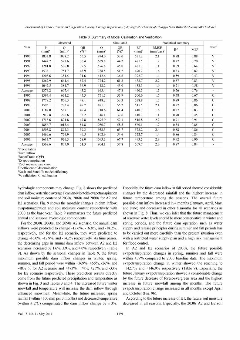
3.1 SWAT Calibration and Validation

Based on the DEM, the watershed was divided into 25 subbasins.

The SWAT model was calibrated for 10 years (1997-2006) daily

streamflow records and validated for another 7 years (1990-1996).

The calibration of streamflow was performed in two steps. First,

the long-term balance was calibrated to match the total flow,

peak flow and base flow by minimizing the difference in average

annual flows. Second, the daily observed and simulated flow

data was calibrated by Nash and Sutcliffe Model Efficiency (ME)

(Nash and Sutcliffe, 1970), coefficients of determination (R2) and

Root Mean Square Error (RMSE).

Table 7 shows the calibrated parameters comparing with the

values of other four studies. Fig. 6 and Fig. 7 show the observed

versus simulated dam inflow for calibration and validation

periods, respectively and a statistical summary is shown in Table

8. The simulated runoff ratio was somewhat overestimated for

the calibration and validation periods. The ME ranged from 0.43

to 0.91, the coefficients of determination ranged from 0.59 to

0.92, and the root mean square error ranged from 1.0 to 2.9 mm.

Then the values for ME and R2 are equal to one, the model

prediction is considered to be perfect. The ME values imply that

the model predicted from 43% to 91% better than using the

average dam inflow value during the study period.

3.2 Hydrologic Impacts by Future Climate Change Con-

sidering Vegetation Canopy Change

For the evaluation of climate and vegetation canopy change

impact on dam inflow, the SWAT model was run with the future

downscaled climate data and the future predicted MODIS LAI

vegetation information. A key for long-term planning and

management of water resources considering future changes in

the pattern of climate, water demand and water availability in a

watershed is not only the possible changes to annual hydrologic

components under climate changes but also how seasonal

Table 7. The Calibrated Parameters for the SWAT Model

Parametername

Description Range This studyZhang(2007)

Heuvelmans et al. (2006)

Muleta and Nicklow (2005)

Bärlund et al.

(2007)

CN2 Curve number adjustment ratio 0 ~ 10 −8 −4 ~ +2(forest)

55- −16 ~ +24

CH_K2Effective hydraulic conductivity in main

channel alluvium (mm/hr)0 ~ 50 50 - - - -

ESCO Soil evaporation compensation 0 ~ 1 0.2 0.4 - 0.0882 -

EPCO Plant uptake compensation factor 0 ~ 1 0.2 0.2 - 1 -

ALPHA_BF Base flow recession constant 0 ~ 1 0.2 0.43 0.5 - 0.15~0.46

SMFMX Maximum snowmelt factor 0 ~ 10 6 8.3 -0.2 - -

SMFMN Minimum snowmelt factor 0 ~ 10 2 5.5 -0.1 - -

TIMP Snow pack temperature lag factor 0 ~ 1 0.5 - 0.5 - -

SNOCOVMXThreshold depth of snow, above which

there is 100% cover0 ~ 500 50 - 10 - -

SNO50COVFraction of snow volume represented by SNOCOVMX that corresponds to 50%

snow cover0 ~ 1 0.5 - - - -

GW_REVAPCoefficient controlling water movement between root zone and shallow aquifer

0.02 ~ 0.2 0.2 - - - 0.10 ~0.18

REVAPMNThreshold depth of water in the shallow

aquifer for ‘re-evap’ to occur (mm)0 ~ 500 400 - - 28.2478 0 ~45

Fig. 6. Calibration Results (1997-2006)

Fig. 7. Validation Results (1990-1996)


Vol. 18, No. 4 / May 2014 − 1191 −

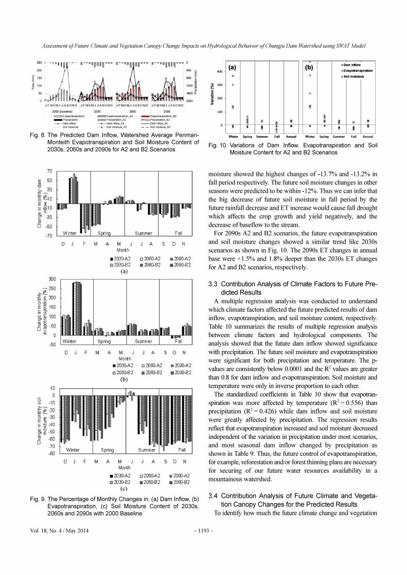
hydrologic components may change. Fig. 8 shows the predicted

dam inflow, watershed average Penman-Monteith evapotranspiration

and soil moisture content of 2030s, 2060s and 2090s for A2 and

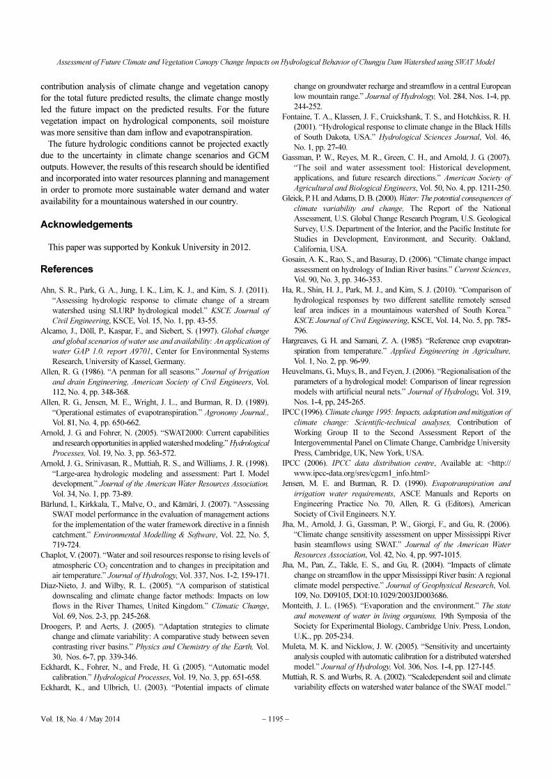
B2 scenarios. Fig. 9 shows the monthly changes in dam inflow,

evapotranspiration and soil moisture content respectively with

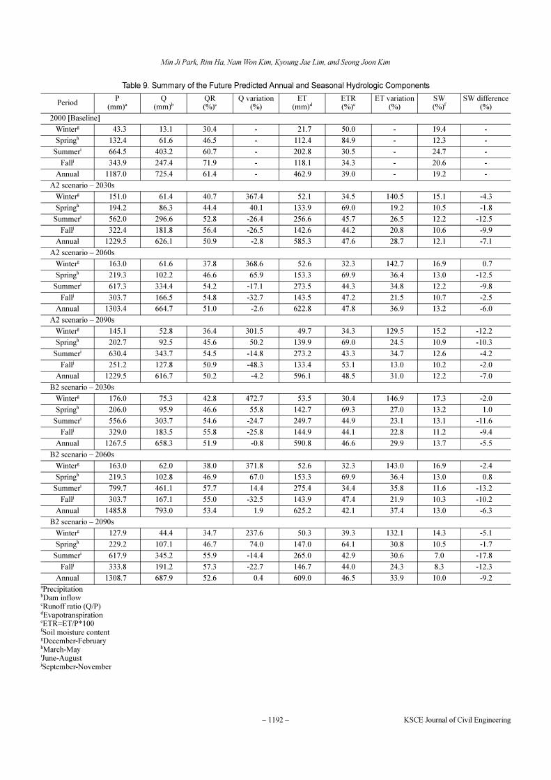
2000 as the base year. Table 9 summarizes the future predicted

annual and seasonal hydrologic components.

For the 2030s, 2060s, and 2090s A2 scenario, the annual dam

inflows were predicted to change -17.6%, -16.8%, and -18.2%,

respectively, and for the B2 scenario, they were predicted to

change -16.0%, -12.9%, and -14.2% respectively. As time passes,

the decreasing gaps in annual dam inflow between A2 and B2

scenarios increased by 1.6%, 3.9%, and 4.0%, respectively (Table

9). As shown by the seasonal changes in Table 9, the future

maximum possible dam inflow changes in winter, spring,

summer, and fall period were within +369%, +66%, -26%, and

-48% % for A2 scenario and +473%, +74%, ±25%, and -33%

for B2 scenario respectively. These prediction results directly

come from the future predicted precipitation and temperature as

shown in Fig. 3 and Tables 3 and 4. The increased future winter

snowfall and temperature will increase the dam inflow through

enhanced snowmelt. Meanwhile, the future increased spring

rainfall (within +100 mm per 3 months) and decreased temperature

(within ± 2oC) compensated the dam inflow change by ± 3%.

Especially, the future dam inflow in fall period showed considerable

changes by the decreased rainfall and the highest increase in

future temperature among the seasons. The overall future

possible dam inflow increased in 4 months (January, April, May,

and June) and decreased in other 8 months for all scenarios as

shown in Fig. 8. Thus, we can infer that the future management

of reservoir water levels should be more conservative in winter and

spring periods, and the future dam operation such as water

supply and release principles during summer and fall periods has

to be carried out more carefully than the present situation even

with a restricted water supply plan and a high risk management

for flood control.

In A2 and B2 scenarios of 2030s, the future possible

evapotranspiration changes in spring, summer and fall were

within +39% compared to 2000 baseline data. The maximum

evapotranspiration change in winter showed the reaching to

+142.7% and +146.9% respectively (Table 9). Especially, the

future January evapotranspiration showed a considerable change

by the future decrease of forest-evergreen area and the highest

increase in future snowfall among the months. The future

evapotranspiration change increased in all months except April

and October (Fig. 9b).

According to the future increase of ET, the future soil moisture

decreased in all seasons. Especially, the 2030s A2 and B2 soil

Table 8. Summary of Model Calibration and Verification

Year

Observed Simulated Statistical summary

NotehP (mm)a

Q(mm)b

QR (%)c

Q(mm)b

QR(%)b

ET(mm)d

RMSE(mm/day)e

R2f MEg

1990 1837.8 1038.2 56.5 974.0 53.0 531.2 2.1 0.88 0.88 V

1991 1447.7 527.6 36.4 639.8 44.2 481.5 1.2 0.77 0.70 V

1992 1281.8 506.8 39.5 576.8 45.0 481.7 1.1 0.69 0.64 V

1993 1538.1 751.7 48.9 788.5 51.2 470.2 1.6 0.83 0.82 V

1994 1208.6 381.5 31.6 442.6 36.6 392.7 1.4 0.59 0.43 V

1995 1262.9 661.4 52.4 774.2 61.3 433.7 2.2 0.87 0.83 V

1996 1042.5 384.7 36.9 448.2 43.0 432.5 1.0 0.71 0.58 V

Average 1374.2 607.4 43.2 663.4 47.8 460.5 1.5 0.76 0.76 -

1997 1394.4 631.2 45.3 751.5 53.9 500.6 1.7 0.78 0.67 C

1998 1778.2 856.3 48.1 948.2 53.3 538.8 1.7 0.89 0.86 C

1999 1595.1 792.4 49.7 881.3 55.2 515.5 2.1 0.87 0.86 C

2000 1187.0 587.1 49.4 718.6 61.4 410.7 1.6 0.87 0.83 C

2001 919.8 296.6 32.2 346.1 37.6 410.7 1.1 0.70 0.45 C

2002 1718.6 821.8 47.8 895.9 52.1 516.8 2.2 0.91 0.91 C

2003 1856.7 1018.4 54.8 1086.7 58.5 560.1 1.7 0.84 0.85 C

2004 1503.8 892.3 59.3 958.5 63.7 528.2 2.4 0.88 0.86 C

2005 1469.6 726.9 49.5 802.9 54.6 522.7 1.4 0.86 0.84 C

2006 1613.7 936.3 58.0 1093.3 67.7 493.5 2.9 0.92 0.90 C

Average 1568.6 807.0 51.3 904.1 57.8 509.7 2.0 0.87 0.84 -aPrecipitationbDam inflowcRunoff ratio (Q/P)dEvapotranspiration eRoot mean square errorfCoefficient of determinationgNash and Sutcliffe model efficiency hV: validation; C: calibration



Table 9. Summary of the Future Predicted Annual and Seasonal Hydrologic Components

PeriodP

(mm)aQ

(mm)bQR(%)c

Q variation(%)

ET(mm)d

ETR(%)e

ET variation(%)

SW(%)f

SW difference(%)

2000 [Baseline]

Winterg 43.3 13.1 30.4 - 21.7 50.0 - 19.4 -

Springh 132.4 61.6 46.5 - 112.4 84.9 - 12.3 -

Summeri 664.5 403.2 60.7 - 202.8 30.5 - 24.7 -

Fallj 343.9 247.4 71.9 - 118.1 34.3 - 20.6 -

Annual 1187.0 725.4 61.4 - 462.9 39.0 - 19.2 -

A2 scenario – 2030s

Winterg 151.0 61.4 40.7 367.4 52.1 34.5 140.5 15.1 -4.3

Springh 194.2 86.3 44.4 40.1 133.9 69.0 19.2 10.5 -1.8

Summeri 562.0 296.6 52.8 -26.4 256.6 45.7 26.5 12.2 -12.5

Fallj 322.4 181.8 56.4 -26.5 142.6 44.2 20.8 10.6 -9.9

Annual 1229.5 626.1 50.9 -2.8 585.3 47.6 28.7 12.1 -7.1


Winterg 163.0 61.6 37.8 368.6 52.6 32.3 142.7 16.9 0.7

Springh 219.3 102.2 46.6 65.9 153.3 69.9 36.4 13.0 -12.5

Summeri 617.3 334.4 54.2 -17.1 273.5 44.3 34.8 12.2 -9.8

Fallj 303.7 166.5 54.8 -32.7 143.5 47.2 21.5 10.7 -2.5

Annual 1303.4 664.7 51.0 -2.6 622.8 47.8 36.9 13.2 -6.0


Winterg 145.1 52.8 36.4 301.5 49.7 34.3 129.5 15.2 -12.2

Springh 202.7 92.5 45.6 50.2 139.9 69.0 24.5 10.9 -10.3

Summeri 630.4 343.7 54.5 -14.8 273.2 43.3 34.7 12.6 -4.2

Fallj 251.2 127.8 50.9 -48.3 133.4 53.1 13.0 10.2 -2.0

Annual 1229.5 616.7 50.2 -4.2 596.1 48.5 31.0 12.2 -7.0

B2 scenario – 2030s

Winterg 176.0 75.3 42.8 472.7 53.5 30.4 146.9 17.3 -2.0

Springh 206.0 95.9 46.6 55.8 142.7 69.3 27.0 13.2 1.0

Summeri 556.6 303.7 54.6 -24.7 249.7 44.9 23.1 13.1 -11.6

Fallj 329.0 183.5 55.8 -25.8 144.9 44.1 22.8 11.2 -9.4

Annual 1267.5 658.3 51.9 -0.8 590.8 46.6 29.9 13.7 -5.5


Winterg 163.0 62.0 38.0 371.8 52.6 32.3 143.0 16.9 -2.4

Springh 219.3 102.8 46.9 67.0 153.3 69.9 36.4 13.0 0.8

Summeri 799.7 461.1 57.7 14.4 275.4 34.4 35.8 11.6 -13.2

Fallj 303.7 167.1 55.0 -32.5 143.9 47.4 21.9 10.3 -10.2

Annual 1485.8 793.0 53.4 1.9 625.2 42.1 37.4 13.0 -6.3


Winterg 127.9 44.4 34.7 237.6 50.3 39.3 132.1 14.3 -5.1

Springh 229.2 107.1 46.7 74.0 147.0 64.1 30.8 10.5 -1.7

Summeri 617.9 345.2 55.9 -14.4 265.0 42.9 30.6 7.0 -17.8

Fallj 333.8 191.2 57.3 -22.7 146.7 44.0 24.3 8.3 -12.3

Annual 1308.7 687.9 52.6 0.4 609.0 46.5 33.9 10.0 -9.2aPrecipitationbDam inflowcRunoff ratio (Q/P)dEvapotranspirationeETR=ET/P*100fSoil moisture contentgDecember-FebruaryhMarch-MayiJune-AugustjSeptember-November


Vol. 18, No. 4 / May 2014 − 1193 −

moisture showed the highest changes of -13.7% and -13.2% in

fall period respectively. The future soil moisture changes in other

seasons were predicted to be within -12%. Thus we can infer that

the big decrease of future soil moisture in fall period by the

future rainfall decrease and ET increase would cause fall drought

which affects the crop growth and yield negatively, and the

decrease of baseflow to the stream.

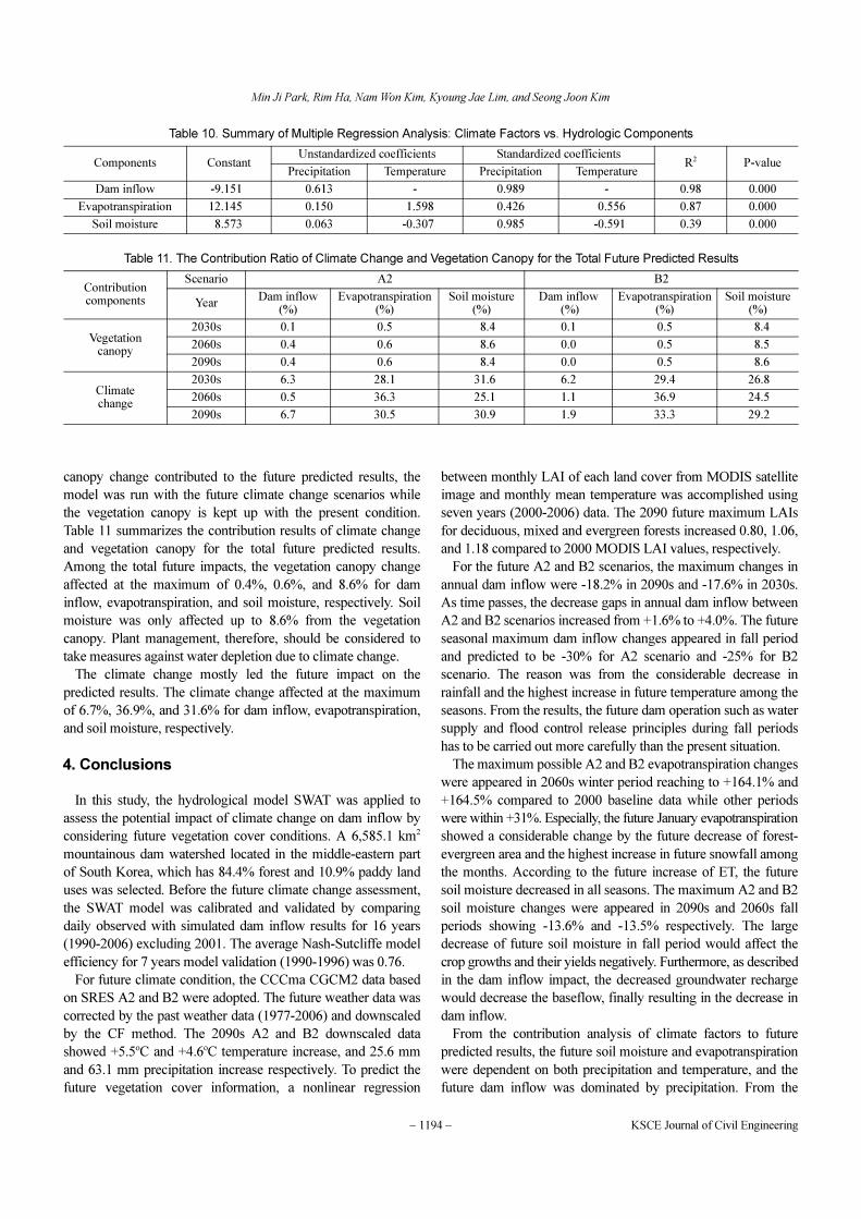
For 2090s A2 and B2 scenarios, the future evapotranspiration

and soil moisture changes showed a similar trend like 2030s

scenarios as shown in Fig. 10. The 2090s ET changes in annual

base were +1.5% and 1.8% deeper than the 2030s ET changes

for A2 and B2 scenarios, respectively.

3.3 Contribution Analysis of Climate Factors to Future Pre-

dicted Results

A multiple regression analysis was conducted to understand

which climate factors affected the future predicted results of dam

inflow, evapotranspiration, and soil moisture content, respectively.

Table 10 summarizes the results of multiple regression analysis

between climate factors and hydrological components. The

analysis showed that the future dam inflow showed significance

with precipitation. The future soil moisture and evapotranspiration

were significant for both precipitation and temperature. The p-

values are consistently below 0.0001 and the R2 values are greater

than 0.8 for dam inflow and evapotranspiration. Soil moisture and

temperature were only in inverse proportion to each other.

The standardized coefficients in Table 10 show that evapotran-

spiration was more affected by temperature (R2 = 0.556) than

precipitation (R2 = 0.426) while dam inflow and soil moisture

were greatly affected by precipitation. The regression results

reflect that evapotranspiration increased and soil moisture decreased

independent of the variation in precipitation under most scenarios,

and most seasonal dam inflow changed by precipitation as

shown in Table 9. Thus, the future control of evapotranspiration,

for example, reforestation and/or forest thinning plans are necessary

for securing of our future water resources availability in a

mountainous watershed.

3.4 Contribution Analysis of Future Climate and Vegeta-

tion Canopy Changes for the Predicted Results

To identify how much the future climate change and vegetation

Fig. 8. The Predicted Dam Inflow, Watershed Average Penman-

Monteith Evapotranspiration and Soil Moisture Content of

2030s, 2060s and 2090s for A2 and B2 Scenarios

Fig. 9. The Percentage of Monthly Changes in: (a) Dam Inflow, (b)

Evapotranspiration, (c) Soil Moisture Content of 2030s,

2060s and 2090s with 2000 Baseline

Fig. 10 Variations of Dam Inflow, Evapotranspiration and Soil

Moisture Content for A2 and B2 Scenarios



canopy change contributed to the future predicted results, the

model was run with the future climate change scenarios while

the vegetation canopy is kept up with the present condition.

Table 11 summarizes the contribution results of climate change

and vegetation canopy for the total future predicted results.

Among the total future impacts, the vegetation canopy change

affected at the maximum of 0.4%, 0.6%, and 8.6% for dam

inflow, evapotranspiration, and soil moisture, respectively. Soil

moisture was only affected up to 8.6% from the vegetation

canopy. Plant management, therefore, should be considered to

take measures against water depletion due to climate change.

The climate change mostly led the future impact on the

predicted results. The climate change affected at the maximum

of 6.7%, 36.9%, and 31.6% for dam inflow, evapotranspiration,

and soil moisture, respectively.

4. Conclusions

In this study, the hydrological model SWAT was applied to

assess the potential impact of climate change on dam inflow by

considering future vegetation cover conditions. A 6,585.1 km2

mountainous dam watershed located in the middle-eastern part

of South Korea, which has 84.4% forest and 10.9% paddy land

uses was selected. Before the future climate change assessment,

the SWAT model was calibrated and validated by comparing

daily observed with simulated dam inflow results for 16 years

(1990-2006) excluding 2001. The average Nash-Sutcliffe model

efficiency for 7 years model validation (1990-1996) was 0.76.

For future climate condition, the CCCma CGCM2 data based

on SRES A2 and B2 were adopted. The future weather data was

corrected by the past weather data (1977-2006) and downscaled

by the CF method. The 2090s A2 and B2 downscaled data

showed +5.5oC and +4.6oC temperature increase, and 25.6 mm

and 63.1 mm precipitation increase respectively. To predict the

future vegetation cover information, a nonlinear regression

between monthly LAI of each land cover from MODIS satellite

image and monthly mean temperature was accomplished using

seven years (2000-2006) data. The 2090 future maximum LAIs

for deciduous, mixed and evergreen forests increased 0.80, 1.06,

and 1.18 compared to 2000 MODIS LAI values, respectively.

For the future A2 and B2 scenarios, the maximum changes in

annual dam inflow were -18.2% in 2090s and -17.6% in 2030s.

As time passes, the decrease gaps in annual dam inflow between

A2 and B2 scenarios increased from +1.6% to +4.0%. The future

seasonal maximum dam inflow changes appeared in fall period

and predicted to be -30% for A2 scenario and -25% for B2

scenario. The reason was from the considerable decrease in

rainfall and the highest increase in future temperature among the

seasons. From the results, the future dam operation such as water

supply and flood control release principles during fall periods

has to be carried out more carefully than the present situation.

The maximum possible A2 and B2 evapotranspiration changes

were appeared in 2060s winter period reaching to +164.1% and

+164.5% compared to 2000 baseline data while other periods

were within +31%. Especially, the future January evapotranspiration

showed a considerable change by the future decrease of forest-

evergreen area and the highest increase in future snowfall among

the months. According to the future increase of ET, the future

soil moisture decreased in all seasons. The maximum A2 and B2

soil moisture changes were appeared in 2090s and 2060s fall

periods showing -13.6% and -13.5% respectively. The large

decrease of future soil moisture in fall period would affect the

crop growths and their yields negatively. Furthermore, as described

in the dam inflow impact, the decreased groundwater recharge

would decrease the baseflow, finally resulting in the decrease in

dam inflow.

From the contribution analysis of climate factors to future

predicted results, the future soil moisture and evapotranspiration

were dependent on both precipitation and temperature, and the

future dam inflow was dominated by precipitation. From the

Table 10. Summary of Multiple Regression Analysis: Climate Factors vs. Hydrologic Components

Components ConstantUnstandardized coefficients Standardized coefficients

R2 P-valuePrecipitation Temperature Precipitation Temperature

Dam inflow -9.151 0.613 - 0.989 - 0.98 0.000

Evapotranspiration 12.145 0.150 1.598 0.426 0.556 0.87 0.000

Soil moisture 8.573 0.063 -0.307 0.985 -0.591 0.39 0.000

Table 11. The Contribution Ratio of Climate Change and Vegetation Canopy for the Total Future Predicted Results

Contributioncomponents

Scenario A2 B2

YearDam inflow

(%)Evapotranspiration

(%)Soil moisture

(%)Dam inflow

(%)Evapotranspiration

(%)Soil moisture

(%)

Vegetation canopy

2030s 0.1 0.5 8.4 0.1 0.5 8.4

2060s 0.4 0.6 8.6 0.0 0.5 8.5

2090s 0.4 0.6 8.4 0.0 0.5 8.6

Climate change

2030s 6.3 28.1 31.6 6.2 29.4 26.8

2060s 0.5 36.3 25.1 1.1 36.9 24.5

2090s 6.7 30.5 30.9 1.9 33.3 29.2


Vol. 18, No. 4 / May 2014 − 1195 −

contribution analysis of climate change and vegetation canopy

for the total future predicted results, the climate change mostly

led the future impact on the predicted results. For the future

vegetation impact on hydrological components, soil moisture

was more sensitive than dam inflow and evapotranspiration.

The future hydrologic conditions cannot be projected exactly

due to the uncertainty in climate change scenarios and GCM

outputs. However, the results of this research should be identified

and incorporated into water resources planning and management

in order to promote more sustainable water demand and water

availability for a mountainous watershed in our country.

Acknowledgements

This paper was supported by Konkuk University in 2012.

References

Ahn, S. R., Park, G. A., Jung, I. K., Lim, K. J., and Kim, S. J. (2011).

“Assessing hydrologic response to climate change of a stream

watershed using SLURP hydrological model.” KSCE Journal of

Civil Engineering, KSCE, Vol. 15, No. 1, pp. 43-55.

Alcamo, J., Döll, P., Kaspar, F., and Siebert, S. (1997). Global change

and global scenarios of water use and availability: An application of

water GAP 1.0. report A9701, Center for Environmental Systems

Research, University of Kassel, Germany.

Allen, R. G. (1986). “A penman for all seasons.” Journal of Irrigation

and drain Engineering, American Society of Civil Engineers, Vol.

112, No. 4, pp. 348-368.

Allen, R. G., Jensen, M. E., Wright, J. L., and Burman, R. D. (1989).

“Operational estimates of evapotranspiration.” Agronomy Journal.,

Vol. 81, No. 4, pp. 650-662.

Arnold, J. G. and Fohrer, N. (2005). “SWAT2000: Current capabilities

and research opportunities in applied watershed modeling.” Hydrological

Processes, Vol. 19, No. 3, pp. 563-572.

Arnold, J. G., Srinivasan, R., Muttiah, R. S., and Williams, J. R. (1998).

“Large-area hydrologic modeling and assessment: Part I. Model

development.” Journal of the American Water Resources Association.

Vol. 34, No. 1, pp. 73-89.

Bärlund, I., Kirkkala, T., Malve, O., and Kämäri, J. (2007). “Assessing

SWAT model performance in the evaluation of management actions

for the implementation of the water framework directive in a finnish

catchment.” Environmental Modelling & Software, Vol. 22, No. 5,

719-724.

Chaplot, V. (2007). “Water and soil resources response to rising levels of

atmospheric CO2 concentration and to changes in precipitation and

air temperature.” Journal of Hydrology, Vol. 337, Nos. 1-2, 159-171.

Diaz-Nieto, J. and Wilby, R. L. (2005). “A comparison of statistical

downscaling and climate change factor methods: Impacts on low

flows in the River Thames, United Kingdom.” Climatic Change,

Vol. 69, Nos. 2-3, pp. 245-268.

Droogers, P. and Aerts, J. (2005). “Adaptation strategies to climate

change and climate variability: A comparative study between seven

contrasting river basins.” Physics and Chemistry of the Earth, Vol.

30, Nos. 6-7, pp. 339-346.

Eckhardt, K., Fohrer, N., and Frede, H. G. (2005). “Automatic model

calibration.” Hydrological Processes, Vol. 19, No. 3, pp. 651-658.

Eckhardt, K., and Ulbrich, U. (2003). “Potential impacts of climate

change on groundwater recharge and streamflow in a central European

low mountain range.” Journal of Hydrology, Vol. 284, Nos. 1-4, pp.

244-252.

Fontaine, T. A., Klassen, J. F., Cruickshank, T. S., and Hotchkiss, R. H.

(2001). “Hydrological response to climate change in the Black Hills

of South Dakota, USA.” Hydrological Sciences Journal, Vol. 46,

No. 1, pp. 27-40.

Gassman, P. W., Reyes, M. R., Green, C. H., and Arnold, J. G. (2007).

“The soil and water assessment tool: Historical development,

applications, and future research directions.” American Society of

Agricultural and Biological Engineers, Vol. 50, No. 4, pp. 1211-250.

Gleick, P. H. and Adams, D. B. (2000). Water: The potential consequences of

climate variability and change, The Report of the National

Assessment, U.S. Global Change Research Program, U.S. Geological

Survey, U.S. Department of the Interior, and the Pacific Institute for

Studies in Development, Environment, and Security. Oakland,

California, USA.

Gosain, A. K., Rao, S., and Basuray, D. (2006). “Climate change impact

assessment on hydrology of Indian River basins.” Current Sciences,

Vol. 90, No. 3, pp. 346-353.

Ha, R., Shin, H. J., Park, M. J., and Kim, S. J. (2010). “Comparison of

hydrological responses by two different satellite remotely sensed

leaf area indices in a mountainous watershed of South Korea.”

KSCE Journal of Civil Engineering, KSCE, Vol. 14, No. 5, pp. 785-

796.

Hargreaves, G. H. and Samani, Z. A. (1985). “Reference crop evapotran-

spiration from temperature.” Applied Engineering in Agriculture,

Vol. 1, No. 2, pp. 96-99.

Heuvelmans, G., Muys, B., and Feyen, J. (2006). “Regionalisation of the

parameters of a hydrological model: Comparison of linear regression

models with artificial neural nets.” Journal of Hydrology, Vol. 319,

Nos. 1-4, pp, 245-265.

IPCC (1996). Climate change 1995: Impacts, adaptation and mitigation of

climate change: Scientific-technical analyses, Contribution of

Working Group II to the Second Assessment Report of the

Intergovernmental Panel on Climate Change, Cambridge University

Press, Cambridge, UK, New York, USA.

IPCC (2006). IPCC data distribution centre, Available at: <http://

www.ipcc-data.org/sres/cgcm1_info.html>

Jensen, M. E. and Burman, R. D. (1990). Evapotranspiration and

irrigation water requirements, ASCE Manuals and Reports on

Engineering Practice No. 70, Allen, R. G. (Editors), American

Society of Civil Engineers. N.Y.

Jha, M., Arnold, J. G., Gassman, P. W., Giorgi, F., and Gu, R. (2006).

“Climate change sensitivity assessment on upper Mississippi River

basin steamflows using SWAT.” Journal of the American Water

Resources Association, Vol. 42, No. 4, pp. 997-1015.

Jha, M., Pan, Z., Takle, E. S., and Gu, R. (2004). “Impacts of climate

change on streamflow in the upper Mississippi River basin: A regional

climate model perspective.” Journal of Geophysical Research, Vol.

109, No. D09105, DOI:10.1029/2003JD003686.

Monteith, J. L. (1965). “Evaporation and the environment.” The state

and movement of water in living organisms, 19th Symposia of the

Society for Experimental Biology, Cambridge Univ. Press, London,

U.K., pp. 205-234.

Muleta, M. K. and Nicklow, J. W. (2005). “Sensitivity and uncertainty

analysis coupled with automatic calibration for a distributed watershed

model.” Journal of Hydrology, Vol. 306, Nos. 1-4, pp. 127-145.

Muttiah, R. S. and Wurbs, R. A. (2002). “Scaledependent soil and climate

variability effects on watershed water balance of the SWAT model.”



Journal of Hydrology, Vol. 256, Nos. 3-4, pp. 264-285.

Nash, J. E. and Sutcliffe, J. V. (1970). “River flow forecasting through

conceptual models: Part 1 - A discussion of principles.” Journal of

Hydrology, Vol. 10, No. 3, pp. 282-290.

Park, J. Y., M. J. Park, H. K. Joh, H. J. Shin, H. J. Kwon, R. Srinivasan,

and Kim, S. J. (2011). “Assessment of MIROC3.2 hires climate and

CLUE-s land use change impacts on watershed hydrology using

SWAT.” Trans. ASABE, Vol. 54, No. 5, pp. 1713-1724.

Priestley, C. H. B. and Taylor, R. J. (1972). “On the assessment of surface

heat flux and evaporation using large-scale parameters.” Monthly

Weather Review, Vol. 100, No. 2, pp. 81-92.

Rosenberg, N. J., Brown, R. A., Izaurralde, R. C., and Thomson, A. M.

(2003). “Integrated assessment of Hadley Centre (HadCM2) climate

change projections in agricultural productivity and irrigation water

supply in the conterminous united states: I. Climate change scenarios

and impacts on irrigation water supply simulated with the HUMUS

model.” Agricultural and Forest Meteorology, Vol. 117, Nos. 1-2,

pp. 73-96.

Rosenberg, N. J., Epstein, D. L., Wang, D., Vail, L., Srinivasan, R., and

Arnold, J. G. (1999). “Possible impacts of global warming on the

hydrology of the Ogallala aquifer region.” Climate Change, Vol. 42,

No. 4, pp. 677-692.

Ryu, J. H., Lee, J. H., Jeong, S. M., Park, S, K., and Han, K. H. (2011).

“The impacts of climate change on local hydrology and low flow

frequency in the Geum River basin, Korea.” Hydrological Processes,

Vol. 25, No. 22, pp. 3437-3447.

Stonefelt, M. D., Fontaine, T. A., and Hotchkiss, R. H. (2000). “Impacts

of climate change on water yield in the upper Wind River basin.”

Journal of the American Water Resources Association, Vol. 36, No.

2, pp. 321-336.

Takle, E. S., Jha, M., and Anderson, C. J. (2005). “Hydrological cycle in

the upper Mississippi River basin: 20th century simulations by

multiple GCMs.” Geophysical Research Letters, Vol. 32, No. 18, pp.

L18407.1-L18407.5.

Thomson, A. M., Brown, R. A., Rosenberg, N. J., Izaurralde, R. C., Legler,

D. M., and Srinivasan, R. (2003). “Simulated impacts of ElNino/

southern oscillation on United States water resources.” Journal of

the American Water Resources Association, Vol. 39, No. 1, pp. 137-

148.

USDA Soil Conservation Service (USDA-SCS) (1972). National

engineering handbook, Section 4 Hydrology 1972 (Chapters 4-10).

Water Resources Update (2003). Is global climate change research

relevant to Day-to-Day water resources management, No. 124.

Wilby, R. L. and Harris, I. (2006) “A framework for assessing uncertainties

in climate change impacts: Low flow scenarios for the River Thames,

UK.” Water Resources Research.

Zhang, G. H. (2007). “Predicting hydrologic response to climate change

in the Luohe River Basin Using the SWAT model.” Trans. of ASAE.

Vol. 50, No. 3, pp. 901-910.

Documents

Assessment of Future Climate and Vegetation Canopy Change ...envsys.co.kr/~envsys/paper/paper12/Assessment of... · length of 447 m and storage volume of 9.7 million m3. Details for