Embed Size (px)
Citation preview
LCA-8002-5S.2008 August 2008
Assessment of Direct and Indirect GHG Emissions Associated with
Petroleum Fuels For New Fuels Alliance
New Fuels Alliance
LCA.6004.3P.2009 February 2009

i
DISCLAIMER
This report was prepared by Life Cycle Associates, LLC for the New Fuels Alliance. Life Cycle
Associates is not liable to any third parties who might make use of this work. No warranty or
representation, express or implied, is made with respect to the accuracy, completeness, and/or
usefulness of information contained in this report. Finally, no liability is assumed with respect to
the use of, or for damages resulting from the use of, any information, method or process
disclosed in this report. In accepting this report, the reader agrees to these terms.
ACKNOWLEDGEMENT
Life Cycle Associates, LLC performed this study with funding from the New Fuels Alliance.
The New Fuels Alliance Project Manager was Brooke Coleman. The report synthesizes inputs
from several contributors who are also engaged in other aspects of life cycle analysis of
petroleum fuels for university research institutions. The following individuals contributed to the
components of the report indicated below with contributions to individual sections being
independent of the overall report. The conclusions and recommendations are those of Life Cycle
Associates, LLC alone.
Stefan Unnasch, Ralf Wiesenberg, Susan Tarka Sanchez, Life Cycle Associates – Petroleum
analysis, economic impacts, project integration, conclusions, and recommendations.
Adam Brandt, PhD Candidate, U.C. Berkeley – Thermally enhanced oil recovery, off shore
drilling, conventional petroleum extraction.
Steffen Mueller, Principal Research Economist Research Assistant Professor, University of
Illinois, Chicago – Iraq reconstruction.
Richard Plevin, PhD Candidate, U.C. Berkeley – Protection of oil supply, land use effects of
forest roads.
Recommended Citation: Unnasch. S., et al. (2009). ―Assessment of Life Cycle GHG Emissions
Associated with Petroleum Fuels,‖ Life Cycle Associates Report LCA-6004-3P. 2009. Prepared
for New Fuels Alliance.
i| Life Cycle Associates, LLC
Summary
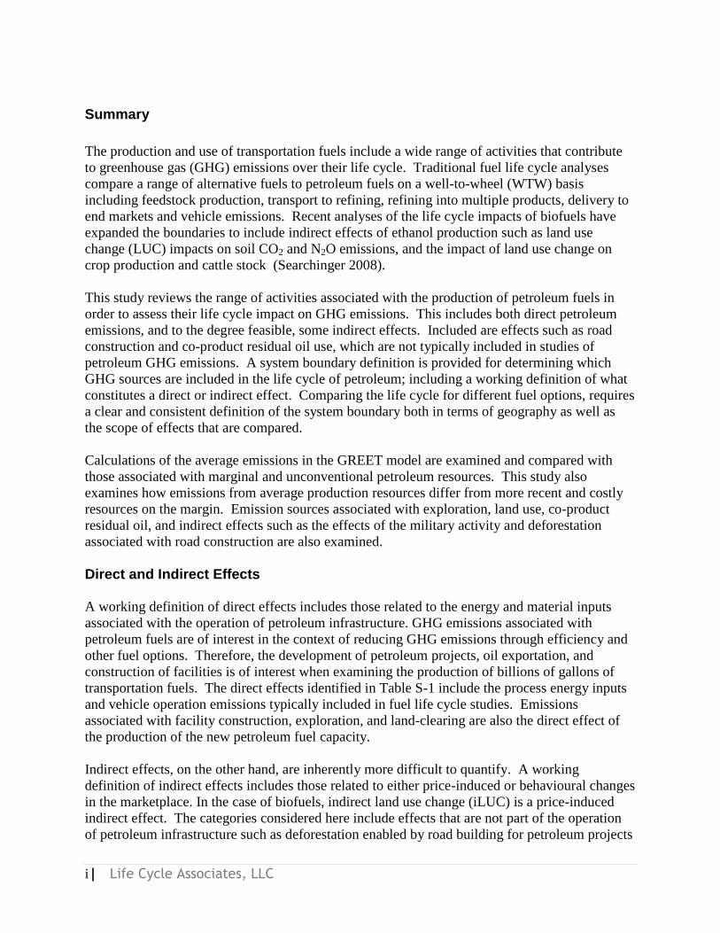
The production and use of transportation fuels include a wide range of activities that contribute
to greenhouse gas (GHG) emissions over their life cycle. Traditional fuel life cycle analyses
compare a range of alternative fuels to petroleum fuels on a well-to-wheel (WTW) basis
including feedstock production, transport to refining, refining into multiple products, delivery to
end markets and vehicle emissions. Recent analyses of the life cycle impacts of biofuels have
expanded the boundaries to include indirect effects of ethanol production such as land use
change (LUC) impacts on soil CO2 and N2O emissions, and the impact of land use change on
crop production and cattle stock (Searchinger 2008).
This study reviews the range of activities associated with the production of petroleum fuels in
order to assess their life cycle impact on GHG emissions. This includes both direct petroleum
emissions, and to the degree feasible, some indirect effects. Included are effects such as road
construction and co-product residual oil use, which are not typically included in studies of
petroleum GHG emissions. A system boundary definition is provided for determining which
GHG sources are included in the life cycle of petroleum; including a working definition of what
constitutes a direct or indirect effect. Comparing the life cycle for different fuel options, requires
a clear and consistent definition of the system boundary both in terms of geography as well as
the scope of effects that are compared.
Calculations of the average emissions in the GREET model are examined and compared with
those associated with marginal and unconventional petroleum resources. This study also
examines how emissions from average production resources differ from more recent and costly
resources on the margin. Emission sources associated with exploration, land use, co-product
residual oil, and indirect effects such as the effects of the military activity and deforestation
associated with road construction are also examined.
Direct and Indirect Effects
A working definition of direct effects includes those related to the energy and material inputs
associated with the operation of petroleum infrastructure. GHG emissions associated with
petroleum fuels are of interest in the context of reducing GHG emissions through efficiency and
other fuel options. Therefore, the development of petroleum projects, oil exportation, and
construction of facilities is of interest when examining the production of billions of gallons of
transportation fuels. The direct effects identified in Table S-1 include the process energy inputs
and vehicle operation emissions typically included in fuel life cycle studies. Emissions
associated with facility construction, exploration, and land-clearing are also the direct effect of
the production of the new petroleum fuel capacity.
Indirect effects, on the other hand, are inherently more difficult to quantify. A working
definition of indirect effects includes those related to either price-induced or behavioural changes
in the marketplace. In the case of biofuels, indirect land use change (iLUC) is a price-induced
indirect effect. The categories considered here include effects that are not part of the operation
of petroleum infrastructure such as deforestation enabled by road building for petroleum projects

ii| Life Cycle Associates, LLC
or military activities that are attributed to the protection of oil supplies. The use of refinery co-
products also has an indirect effect on energy markets.
Table S-1 examines to what extent direct and indirect emissions have been included in petroleum
fuel life cycle analyses. Traditional fuel cycle analyses focus on average oil production, refining,
transport and vehicle use. Some studies also examine the requirements for heavy oil and oil
sands production. The energy inputs and emissions associated with oil exploration are typically
not examined. In circumstances such as Californian and Canadian oil resources, the location of
oil resources has been established for decades. However, new off shore oil resources require
ongoing exploration activities and more energy-intensive extraction technologies. The energy
inputs and emissions associated with the production, refining and transport of petroleum often
reflect the average petroleum infrastructure. However, considerable variation in energy
requirements is apparent in crude types; thus at a minimum, the range in GHG emissions
associated with petroleum infrastructure is understated.
The question of refinery emissions is a more complex topic because of the range of inputs,
transportation of fuel products, and heavy co-products. Processing requirements vary with crude
oil sulphur content, gravity (also related to carbon content), and other aspects of its assay.
Considerably more analysis is needed to properly partition emissions within the oil refinery and
understand the effects of different crude types. Since oil refining is such a complex process, it is
not surprising that a consistent approach for treating oil refining is not applied among different
life cycle studies.
The impacts of facility construction are often considered comparable among fuel options.
However, oil exploration and land clearing associated with oil sands are unique to the petroleum
industry. In order to provide a consistent representation of the inputs used to produce petroleum
fuels, the emissions associated with these activities should be included in life cycle assessments
in a clear and comparable manner.
Military activities associated with the protection of oil supply are often attributed to the use of
gasoline. The emissions associated with the protection of oil supply are categorized as indirect
effects because there is no straightforward approach to relating a direct process throughput with
military activity. The effects of protection of oil supply can include military activities in the
Middle East, the effects of the Iraq wars, as well and the post war effects on both reconstruction
and U.S. troops. However, it is difficult to agree on an approach for identifying, and quantifying,
the direct vs. indirect effects of military activity.
Additional indirect effects correspond to the use of co-products associated with oil refining. For
example, GHG emissions from residual oil and petroleum coke combustion exceed those from
all of the alternative fuels used in the U.S. today. These emissions are treated with various
allocation schemes in life cycle analyses. The effects of substitute products and the carbon
intensity of petroleum co-products need to be examined further as the modelling approach
requires further scrutiny.

iii| Life Cycle Associates, LLC
Table S-1. Categorization of direct vs. indirect effects of petroleum production.
Petroleum
Supply
Option
Direct Effects Indirect Effects
Oil
Exp
lora
tion
Oil
Pro
du
ctio
n
Met
han
e lo
sses
, fl
ari
ng
Oil
Ref
inin
g
Oil
an
d P
rod
uct
Tra
nsp
ort
Lan
d U
se C
on
ver
sion
Tail
ing l
ak
es, C
H4
Veh
icle
fu
el
Exh
au
st m
inor
spec
ies
Mate
rial
inp
uts
Ref
iner
y C
o-p
rod
uct
s
Macr
o E
con
om
ic E
ffec
ts
Pro
tect
ion
of
oil
su
pp
ly
Iraq
Rec
on
stru
ctio
n
Ind
irec
t la
nd
Use
Venezuelan
Heavy −
Canadian Oil
Sands − −
Iraqi − − − −
Nigerian − − − − −
California
TEOR
−
−
−
U.S. Off
Shore −
−
− −
−
Conventional − − − −
Included in traditionala fuel life cycle analysis
Excluded from traditional fuel life cycle analysis because relative difference among
fuels is small
Not included in traditional full fuel life cycle analyses
Include in traditional fuel life cycle analyses and requires additional study
− Not applicable a Delucchi‘s work on fuel life cycle analysis includes many of the effects in this table
or recommends work in these areas. b Market effects of petroleum would also include induced effects on land use.
Broader economic or price-induced petroleum effects are difficult to systematically assign a
boundary given the prevalence of oil-induced economic drivers in the world economy.
However, to the extent that economic effects are considered a part of the life cycle analysis of
alternative fuels, as is the case with iLUC for biofuels, their effect vis-à-vis petroleum is also of
iv| Life Cycle Associates, LLC
interest. The effect of changes in petroleum supply and price will effect global goods, their
movement, and the use of resources and their related GHG emissions. Petroleum dependence
and oil price fluctuations influence a wide range of worldwide markets, ranging from agricultural
commodity prices to the cost of living and doing business. Economic effects clearly require
further study as market effects have proven to cause more of an effect than government
regulatory measures.
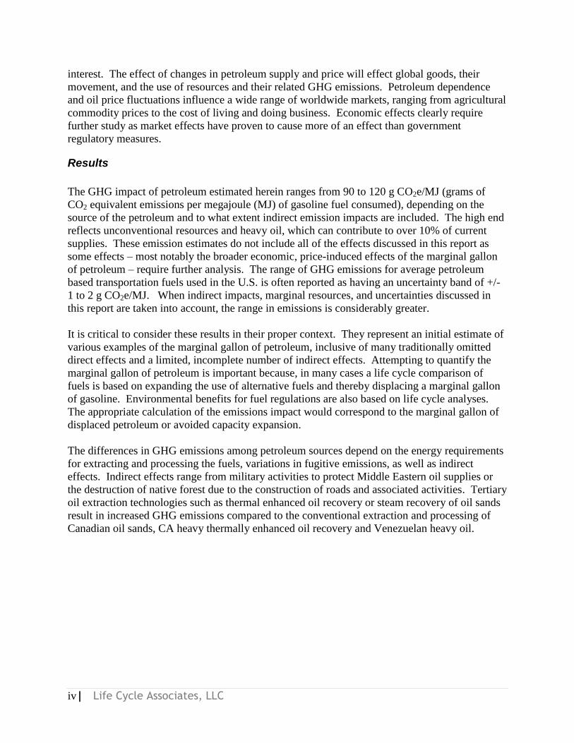
Results
The GHG impact of petroleum estimated herein ranges from 90 to 120 g CO2e/MJ (grams of
CO2 equivalent emissions per megajoule (MJ) of gasoline fuel consumed), depending on the
source of the petroleum and to what extent indirect emission impacts are included. The high end
reflects unconventional resources and heavy oil, which can contribute to over 10% of current
supplies. These emission estimates do not include all of the effects discussed in this report as
some effects – most notably the broader economic, price-induced effects of the marginal gallon
of petroleum – require further analysis. The range of GHG emissions for average petroleum
based transportation fuels used in the U.S. is often reported as having an uncertainty band of +/-
1 to 2 g CO2e/MJ. When indirect impacts, marginal resources, and uncertainties discussed in
this report are taken into account, the range in emissions is considerably greater.
It is critical to consider these results in their proper context. They represent an initial estimate of
various examples of the marginal gallon of petroleum, inclusive of many traditionally omitted
direct effects and a limited, incomplete number of indirect effects. Attempting to quantify the
marginal gallon of petroleum is important because, in many cases a life cycle comparison of
fuels is based on expanding the use of alternative fuels and thereby displacing a marginal gallon
of gasoline. Environmental benefits for fuel regulations are also based on life cycle analyses.
The appropriate calculation of the emissions impact would correspond to the marginal gallon of
displaced petroleum or avoided capacity expansion.
The differences in GHG emissions among petroleum sources depend on the energy requirements
for extracting and processing the fuels, variations in fugitive emissions, as well as indirect
effects. Indirect effects range from military activities to protect Middle Eastern oil supplies or
the destruction of native forest due to the construction of roads and associated activities. Tertiary
oil extraction technologies such as thermal enhanced oil recovery or steam recovery of oil sands
result in increased GHG emissions compared to the conventional extraction and processing of
Canadian oil sands, CA heavy thermally enhanced oil recovery and Venezuelan heavy oil.
v| Life Cycle Associates, LLC
-10
0
10
20
30
40
50
60
70
80
90
100
110
120
Ave
rage
Pet
roleum
U.S
. Off
Sho
re
Califo
rnia T
EOR
Nigeria
n
Iraqi
Can
adian
Oil San
ds
Ven
ezual
a Hea
vy
Gaso
lin
e L
ife C
ycle
GW
I (g
/MJ)
Land Impacts
Heavy Coproducts
Protection of Supply
Refining
Transport
Venting and Flaring
Production
Fuel Combustion
Rebound
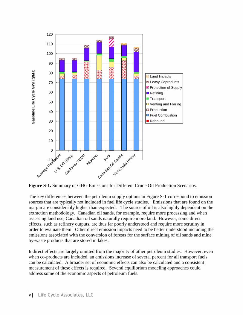
Figure S-1. Summary of GHG Emissions for Different Crude Oil Production Scenarios.
The key differences between the petroleum supply options in Figure S-1 correspond to emission
sources that are typically not included in fuel life cycle studies. Emissions that are found on the
margin are considerably higher than expected. The source of oil is also highly dependent on the
extraction methodology. Canadian oil sands, for example, require more processing and when
assessing land use, Canadian oil sands naturally require more land. However, some direct
effects, such as refinery outputs, are thus far poorly understood and require more scrutiny in
order to evaluate them. Other direct emission impacts need to be better understood including the
emissions associated with the conversion of forests for the surface mining of oil sands and mine
by-waste products that are stored in lakes.
Indirect effects are largely omitted from the majority of other petroleum studies. However, even
when co-products are included, an emissions increase of several percent for all transport fuels
can be calculated. A broader set of economic effects can also be calculated and a consistent
measurement of these effects is required. Several equilibrium modeling approaches could
address some of the economic aspects of petroleum fuels.

vi| Life Cycle Associates, LLC
Conclusions
As depicted in Figure S-1, production of petroleum fuels involves numerous energy and
economic impacts that affect the global GHG emissions associated with fuel consumption.
Many of the impacts of oil production are examined in well published fuel life cycle studies,
which primarily use average energy inputs and emissions. However, the variety of emission
sources associated with petroleum production is often omitted from life cycle studies.
The GHG emissions associated with the production and use of petroleum fuels are still uncertain,
particularly for fuels on the margin. The supply chain requires additional study as many of the
methods used to estimate GHG emissions are still poorly developed. However, co-products and
heavy refining do account for high outputs as can be seen in the case of Venezuela Heavy Crude.
This is also apparent as a result of increased venting and flaring in Nigeria, the protection of oil
in Iraq and the production of Canadian oil sands.
Calculations in this study indicate that the fate of residual oil and petroleum coke is important,
and a potentially significant source of GHG emissions, but require further economic modeling.
The magnitude of carbon emissions associated with these products indicates that a detailed
analysis of their fate and the effect on other fuel markets should be examined.
The definition of a direct vs. indirect effect may remain vague. The debate as to whether the Iraq
war, for example, is an effect that occurs as a direct or indirect result of petroleum dependence
will continue. It could be argued that an indirect effect of the war, and therefore petroleum use,
might include health effects and long term Middle East presence by the western world.
Nonetheless, the magnitude of the emissions directly associated with military activity is readily
calculated. More analysis may improve the readers‘ perspective but opinions are likely to
remain diverse.
Higher oil prices and dwindling light crude stocks induce development of more costly, energy
intensive petroleum resources that have higher than average life cycle GHG emissions. These
marginal supplies are associated with:
Tertiary oil recovery
Production of heavy oils
Production of oil sands derived fuel
Imports of finished product from remote locations in relatively small vessels
Production from small capacity stripper wells
Once projects are completed and operational the oil produced becomes part of the world oil
supply. Hence, the average GHG emissions are expected to increase and new marginal supplies
are likely to have even higher greenhouse emissions. Nonetheless, high cost, energy intensive
marginal resources must be factored into current and future projections of the impact of
petroleum based transportation fuels to the extent that marginal considerations are taken into
account for alternative fuels.
vii| Life Cycle Associates, LLC
Terms and Abbreviations
ANL Argonne National Laboratory
API American Petroleum Institute
bbl Barrel
bcm Billion cubic meters
bhp-h brake horse power-hour
Btu British thermal unit
CEC California Energy Commission
CGE Computational general equilibrium
CH4 Methane
CO2 Carbon dioxide
CPI Consumer Price Index
DC Developing Country
DDGS Dried distillers grains with soluble
DoD Department of Defense
DOE Department of Energy
DWT Deadweight
ECA Emissions Control Areas
EIA Energy Information Administration
EIO-LCA Environmental Input Output Life Cycle Assessment
EPA Environmental Protection Agency
FAPRI Food and Agricultural Policy Research Institute
FASOM Forest and Agricultural Sector Optimization Model
FSU Former Soviet Union
ft Feet
gal Gallon
GEMIS Global Emission Model for Integrated Systems
GHG Greenhouse gas
GM General Motors Corporation
GREET Greenhouse gas, Regulated Emissions and Energy Use
in Transportation (Argonne National Laboratory‘s well-to-wheels model)
GTAP Global Trade Analysis Project
GTL Gas to liquid
GWI Global warming intensity
ha Hectare
H/C Hydrogen/Carbon ratio
HFO Heavy fuel oil
IEA International Energy Agency
IFO Intermediate fuel oil
IMO International Maritime Organization
IPCC Intergovernmental Panel on Climate Change
J Joule
JEC Joint Economic Committee
kJ kilo joule

viii| Life Cycle Associates, LLC
km kilometer
kWh kilowatt hour
LCA Life cycle assessment
LCFS Low Carbon Fuel Standard
LCI Life cycle inventory
LPG Liquefied petroleum gas
LUC Land use change
iLUC Indirect Land use change
Mbbl Million barrels
Mboe Million barrels of oil equivalent
Mg Mega gram, 1 metric ton
MIT Massachusetts Institute of Technology
MJ Mega joule
mm Btu Abbreviation for million Btu for English units
NASA National Aeronautics and Space Administration
NG natural gas
N2O Nitrous oxide
NOAA U.S. National Oceanic and Atmospheric Agency
OECD Organization for Economic Co-operation and Development
OPEC Organization of the Petroleum Exporting Countries
PADD Petroleum Administration for Defense Districts
PJ Peta Joule, 1015
Joules
PwC Price-Waterhouse-Coopers
RBOB Reformulated blend stock for oxygen blending
RCF RCF Consulting of Chicago
RFG Reformulated gasoline
SAGD Steam Assisted Gravity Drainage
SO2 Sulfur Dioxide
UK United Kingdom
UN United Nations
USDOC United Stated Department of Commerce
USAID United States Agency for International Development
U.S. United States
TEOR Thermally enhanced oil recovery
Tg Terra gram, 106 metric tonnes
tonne metric ton, 1000 kg
TTW Tank to wheels
WBCSD World Business Council for Sustainable Development
WTT Well to tank

ix| Life Cycle Associates, LLC
Table of Contents
Summary .......................................................................................................................................... i
1. Introduction ............................................................................................................................. 1
2. Scope of Petroleum Life Cycle Emissions .............................................................................. 5
2.1. System Boundaries.......................................................................................................... 5
2.2. GREET Model Scope ..................................................................................................... 7
2.3. Marginal Impacts .......................................................................................................... 11
2.4. Economic Effects .......................................................................................................... 12
2.4.1. Indirect Impacts of Biofuels and Effect on Indirect Petroleum Effects ................ 13
2.4.2. Direct and Indirect Effects of Petroleum Production ............................................ 14
2.5. Direct Emissions of Petroleum Production ................................................................... 15
2.7. Attribution of Emission to Fuel Production .................................................................. 17
3. Direct Petroleum Production Emissions ............................................................................... 19
3.1. Exploration, Drilling, and Production ........................................................................... 19
3.1.1. Conventional Oil Exploration, Drilling, and Production Data ............................. 19
3.1.2. Offshore Oil Production ........................................................................................ 22
3.1.3. Thermal Enhanced Oil Recovery .......................................................................... 23
3.1.4. Oil Sands Production ............................................................................................ 26
3.1.5. Oil Exploration and Production Recommendations ............................................. 27
3.2. Oil Sands Tailings ......................................................................................................... 27
3.3. Natural Gas Venting and Flaring .................................................................................. 28
3.3.1. Future Trends in Venting and Flaring ................................................................... 30
3.3.2. Venting and Flaring Recommendations................................................................ 32
3.4. Petroleum Refining ....................................................................................................... 33
3.4.1. Conventional Petroleum Refining......................................................................... 34
3.4.2. Heavy Oil and Oil Sands Upgrading .................................................................... 35
3.4.3. Oil Refining Recommendations ............................................................................ 36
3.5. Crude and Product Transport ........................................................................................ 37
3.6. Refinery Co-Products.................................................................................................... 38
3.6.1. Approach to Refinery Co-products ....................................................................... 40
3.6.3. Refinery Co-product Recommendations............................................................... 45
3.7. Economic Impacts ......................................................................................................... 45
3.7.1. Equilibrium Models .............................................................................................. 48
3.7.2. Displacement of Gasoline by Alternatives ........................................................... 49

x| Life Cycle Associates, LLC
3.7.3. Recommendations on Economic Effects .............................................................. 50
3.8. Protection of Petroleum Supply .................................................................................... 50
3.8.1. Greenhouse gas estimate for Iraq war ................................................................... 51
3.8.2. Total military fuel use ........................................................................................... 52
3.8.3. Oil Field Fires ....................................................................................................... 53
3.8.4. Recommendations on Protection of Oil Supply.................................................... 54
3.9. Iraq Reconstruction ....................................................................................................... 54
3.9.1. Cement Production................................................................................................ 54
3.9.2. GHG Emissions from Iraq Reconstruction Efforts ............................................... 56
3.9.3. Recommendations on Iraq Reconstruction ........................................................... 56
4. Land use and other environmental impacts .......................................................................... 56
4.1. Deforestation following road construction ................................................................... 56
4.2. Tar Sands Production and Other Land Use................................................................... 60
4.3. Land Use Recommendations ........................................................................................ 60
5. Impact on Life Cycle Assessment......................................................................................... 61
5.1. Uncertainties ................................................................................................................. 63
6. References ............................................................................................................................. 64
7. Appendix……………………………………………………………………………………74
Lists of Figures and Tables
Tables Table 1. Groupings of Direct and Indirect Emission Effects. ......................................................... 3 Table 2. Project Tasks. .................................................................................................................... 4
Table 3.Treatment of Fuel Cycle Categories for Petroleum Pathways in the GREET Model. .... 10 Table 4. Categorization of direct vs. indirect effects of petroleum production. ........................... 14
Table 5. Direct GHG Effects Due to Petroleum Usage ................................................................ 15 Table 6. Potential Indirect GHG Effects Due to Petroleum Usage. .............................................. 16 Table 7. Example Attribution of Fuel Throughput to Emission Sources. .................................... 17
Table 8. Total U.S. Petroleum and Transport Fuel Consumption, 2003-2007. ............................ 18 Table 9. Economic Census Datasets. ............................................................................................ 19 Table 10. Energy inputs to oil and gas support, drilling, and extraction (J/100J of crude oil
output). .......................................................................................................................................... 20 Table 11. Energy Inputs and GHG Impacts. ................................................................................. 25
Table 12. Estimate of Natural Gas Flaring in Oil Producing Countries. ...................................... 31 Table 13. Impacts of Crude Oil Transportation Mode. ................................................................. 37 Table 14. Energy Inputs and Outputs from U.S. Refineries. ........................................................ 42
Table 15. Protection adder based on Iraq War. ............................................................................. 52
xi| Life Cycle Associates, LLC
Table 16. Protection adder based on Iraq War emissions. ............................................................ 53 Table 17. Oil producing countries with rainforests. Primary oil production for most of these
countries is offshore. Colombia, Ecuador, Peru, Bolivia, and Nigeria have substantial oil
operations in rainforest areas. ....................................................................................................... 58
Table 18. Deforestation on the Colombian Side of the Border..................................................... 59 Table 19. Deforestation on the Ecuadorian Side of the Border. ................................................... 59
Figures
Figure 1. System boundary for petroleum fuel production and vehicle use. .................................. 6 Figure 2. Life cycle impacts occur on the margin as shown by ‗business as usual‘. .................... 11 Figure 3. Oil drilling rig. ............................................................................................................... 22
Figure 4. Oil sands tailing ponds are a potential source of hydrocarbon emissions. Anaerobic
conditions in peat soils could accelerate methane production. ..................................................... 28 Figure 5. Leading countries with flared gas emissions (Source: World Bank). ........................... 29
Figure 6. Modern Oil Refinery. .................................................................................................... 33 Figure 7. Crude Oil Tanker ........................................................................................................... 37
Figure 8. Imports of petroleum products to the U.S. .................................................................... 39 Figure 9. Crude oil volume and transport distance. ...................................................................... 40 Figure 10. Change in residual oil and coke emissions with constant refinery configuration and
changing gasoline output. ............................................................................................................. 44 Figure 11. General model representation of economic impacts (Berk). ....................................... 47
Figure 12. The U.S. military oil consumption and costs (Source: Karbuz 2007). ........................ 52
Figure 13. USAF aircraft fly over Kuwaiti oil fires, set by the retreating Iraqi army during
Operation Desert Storm in 1991. Source www.af.mil/photos on www.wikipedia.com ............... 53 Figure 14. Summary of GHG Emissions for Different Crude Oil Production Scenarios. ............ 62
1| Life Cycle Associates, LLC
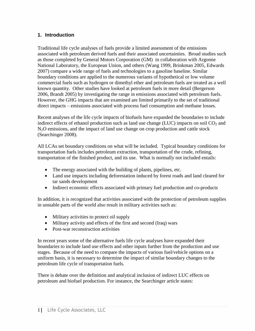
1. Introduction
Traditional life cycle analyses of fuels provide a limited assessment of the emissions
associated with petroleum derived fuels and their associated uncertainties. Broad studies such
as those completed by General Motors Corporation (GM) in collaboration with Argonne
National Laboratory, the European Union, and others (Wang 1999, Brinkman 2005, Edwards
2007) compare a wide range of fuels and technologies to a gasoline baseline. Similar
boundary conditions are applied to the numerous variants of hypothetical or low volume
commercial fuels such as hydrogen or dimethyl ether and petroleum fuels are treated as a well
known quantity. Other studies have looked at petroleum fuels in more detail (Bergerson
2006, Brandt 2005) by investigating the range in emissions associated with petroleum fuels.
However, the GHG impacts that are examined are limited primarily to the set of traditional
direct impacts – emissions associated with process fuel consumption and methane losses.
Recent analyses of the life cycle impacts of biofuels have expanded the boundaries to include
indirect effects of ethanol production such as land use change (LUC) impacts on soil CO2 and
N2O emissions, and the impact of land use change on crop production and cattle stock
(Searchinger 2008).
All LCAs set boundary conditions on what will be included. Typical boundary conditions for
transportation fuels includes petroleum extraction, transportation of the crude, refining,
transportation of the finished product, and its use. What is normally not included entails:
The energy associated with the building of plants, pipelines, etc.
Land use impacts including deforestation induced by forest roads and land cleared for
tar sands development
Indirect economic effects associated with primary fuel production and co-products
In addition, it is recognized that activities associated with the protection of petroleum supplies
in unstable parts of the world also result in military activities such as:
Military activities to protect oil supply
Military activity and effects of the first and second (Iraq) wars
Post-war reconstruction activities
In recent years some of the alternative fuels life cycle analyses have expanded their
boundaries to include land use effects and other inputs further from the production and use
stages. Because of the need to compare the impacts of various fuel/vehicle options on a
uniform basis, it is necessary to determine the impact of similar boundary changes to the
petroleum life cycle of transportation fuels.
There is debate over the definition and analytical inclusion of indirect LUC effects on
petroleum and biofuel production. For instance, the Searchinger article states:

2| Life Cycle Associates, LLC
―The amount of land used to produce a gallon of gasoline is extremely small —
according to some energy experts we have quickly consulted, it is less than 1
percent of the amount of land used to produce a gallon-equivalent of ethanol.
Much of the world’s oil is either produced in deserts or offshore or on land
that still remains in productive agricultural use. Because the effect of oil
production on emissions from land use change is small, it is reasonable to omit
it‖.
Consistency with the intent and significant detail of traditional fuel cycle analyses postulates
inclusion rather than exclusion of ‗insignificant values‘. Moreover, the differences in carbon
intensity between various compliance fuels relative to each other and petroleum in a carbon-
based performance standard is very small, which implies that relatively small effects could be
significant within a carbon-based fuel regulation. Still there is justifiable difficulty in
measuring indirect effects- as they often are not at the capacity level and therefore are often
not physical effects.
The GREET model is inclusive of many of the direct effects of petroleum production, and
calculates these with intense scrutiny and precision. However, some variables such as
Nigerian natural gas flaring of heavy oil production and upgrading in Venezuela are not so
easily measured. Even with GREET covering over 100 fuel production pathways and over 80
vehicle-fuel systems, the emissions from such fuel production scenarios reflect significant
departures from the default GREET inputs.
The debate over life cycle GHG emissions calculations, in terms of what variables to include
and what, if any, to exclude, has prompted this study. The aim is to examine the impact of
expanding the boundary conditions for the production and use of petroleum based
transportation fuels to include a number of direct and indirect effects that are consistent with
the requirements to produce petroleum fuels. A grouping of direct and indirect effects is
shown in Table 1. The categories, developed here, provide a framework for categorizing life
cycle emissions.
The direct effects are related to the primary energy inputs and emissions associated with fuel
production. These include activities that are required to produce an additional unit of fuel,
which include crude oil production, refining, distribution and vehicle end use considered in
traditional fuel cycle analyses. To the extent that this question is interesting in the debate
surrounding fuel options and GHG emissions, direct emissions would include activities
associated with significant usage and therefore would include emissions associated with
finding new oil, clearing land, and building production and refining facilities.
Indirect effects encompass all effects related to fuel production other than the energy and
emission impacts directly associated with feedstock extraction, refining, transport, and vehicle
operation. Many of the indirect effects of fuel production are induced by market forces of
supply and demand. Others may be the consequence of government policy.

3| Life Cycle Associates, LLC
Table 1. Groupings of Direct and Indirect Emission Effects.
Direct Effects
Oil Exploration
Oil Production
Methane losses, flaring
Oil Refining
Oil and Product Transport
Land Use Conversion
Tailing lakes, CH4
Vehicle fuel Exhaust minor species
Material inputs
Indirect Effects
Refinery Co-products
Macro Economic Effects
Protection of oil supply
Iraq Reconstruction
Indirect land Use
Indirect effects can be addressed within the traditional LCA boundary, but fluctuate due to
changing economic conditions and are thereby induced. For example:
Shift to heavier and unconventional crude oil supplies
Price pressures on gasoline with decreased/increased biofuels supply
Price pressures on refinery inputs such as natural gas
Price pressures on agricultural commodities from petroleum prices
Of course there are the indirect effects that are outside the traditional LCA boundary, such as
road building and military activity. Included are:
Emissions from U.S. government military activities in defense of Middle East oil
Increased material use (i.e. cement) for war zone reconstruction
Oil field fires due to military activities
Road building to increase access and therefore increase deforestation
All other effects are grouped as indirect effects, which includes both economic impacts and
other consequences of producing petroleum fuels. Table 4 summarizes the direct and indirect
effects in a structured manner. The categories reflect the authors‘ grouping of the direct
effects that occur with additional throughput or production capacity and are inputs to
petroleum infrastructure. The indirect effects occur because of petroleum production
activities but they are not part of the petroleum supply chain. The framework of petroleum
effects provides the basis for the organization of this report.
The purpose of this study is to examine the direct and indirect effects of petroleum fuels. It
develops a definition of direct and indirect effects, and examines what is included in existing
fuel life cycle models. The study also examines and quantifies emissions that are not widely

4| Life Cycle Associates, LLC
included in fuel life cycle analyses and develops recommendations to provide an improved
understanding of the range of emissions associated with the production and use of petroleum
fuels. This study should not be interpreted to include the full spectrum of indirect effects from
petroleum, as many of the broader economic, price-induced effects are not quantified here
because additional analysis must be conducted to deduce reasonable numerical estimations for
these effects.
A list of the project tasks and the work breakdown structure is given in Table 2. The project
team reviewed the range of emission impacts associated with petroleum production to assess
how petroleum fuels are incorporated in life cycle analysis and what impacts are not included.
First the analysis scope of the GREET model was examined. Then the range of fuel
production impacts were identified and screened to assess their potential magnitude.
Preliminary estimates of the life cycle GHG emissions were calculated. Many of the effects of
petroleum processing include only specific resource options and production pathways, while
others are broadly applicable. The GHG impacts associated with different petroleum
resources and production pathways are then compared with the impacts related to each
pathway.
The impact due to changes in the use of marginal petroleum sources are examined by
investigating a range of petroleum production options. The analysis is framed in the context
of a reduction in petroleum usage that would be consistent with the incremental increase in
biofuels and other alternative fuels in the U.S. This might include an additional 10 billion
gal/year of corn based ethanol and another 20 billion gallons per year of cellulose, sugar cane,
and other biofuel based ethanol. In contrast, many fuel life cycle studies focus on average
emissions. For example, the GREET model‘s default values for petroleum fuels and ethanol
reflect average emissions for the U.S. This study examines how emissions from the average
production resources differ from newer and more costly resources on the margin.
Table 2. Project Tasks.
Task Description
1 System Boundary Definition
Define scope of traditional life cycle analysis
Define average versus marginal analysis requirements
Define direct and indirect impacts of petroleum
2 Life Cycle Inventory Data
Identify scoping calculations for key data gaps
Calculate inputs to determine GHG emissions
Determine process input assumptions
3 Petroleum Production Effects
Calculate direct effects per MJ of fuel
Estimate indirect effects and calculate per MJ fuel
Review market mitigated effects (price elasticity)
Describe complex attribution, driven by assumptions
4 Impact on Life Cycle Assessment
Develop petroleum scenarios
Estimate range of direct and indirect impacts

5| Life Cycle Associates, LLC
2. Scope of Petroleum Life Cycle Emissions
A traditional petroleum production LCA measures the life cycle GHG impacts associated with
the production of petroleum fuels. The calculation methods are applied on a process specific
or regional basis. These calculations present GHG emissions on an intensity basis, thus the
functional unit of analysis is a MJ of gasoline. The life cycle analysis of petroleum is
examined from exploration through vehicle end use, or a well to wheel basis. Both direct and
indirect impacts and co-products are examined. It identifies market mitigated drivers;
however, a much more extensive economic modeling effort is needed to formally assess these
impacts.
A life cycle analysis of petroleum fuels should follow a set of procedures to determine how
the study is conducted1. ISO 14044 (ISO 2006) provides requirement that have been applied
to fuel life cycle studies. Specifically:
ISO 14040 specifies requirements and provides guidelines for life cycle assessment
(LCA) including: definition of the goal and scope of the LCA, the life cycle
inventory analysis (LCI) phase, the life cycle impact assessment (LCIA) phase, the
life cycle interpretation phase, reporting and critical review of the LCA,
limitations of the LCA, relationship between the LCA phases, and conditions for
use of value choices and optional elements.
The first step in a life cycle analysis is to determine the scope of the study and asks the
following three questions:
Why is the study being conducted?
What effects are important?
What emissions are included?
The life cycle of petroleum fuels is generally of interest because the introduction of significant
quantities of alternative fuels are being considered world wide. Government policies,
technology improvements, and other factors are often targeted to displace 10 to over 30% of
petroleum usage, including growth in capacity ((DOE 2008, CEC 2003, RTFO (UK)).
Therefore, the scope of the petroleum life cycle analysis of interest should be consistent with
such large reductions in output.
2.1. System Boundaries
In general, the system boundary for fuel production includes material inputs, resource
extraction, production, vehicle use, and end of life activities. Many fuel life cycle studies
perform a process based analysis that accounts for the direct energy inputs and emissions
associated with fuel production. The process based analysis allows the system boundary to be
drawn tightly and avoids endless smaller secondary material inputs and economic effects. A
1 This scope of this study is not a complete life cycle assessment and is determining what should be
included in the life cycle assessment and what is missing.

6| Life Cycle Associates, LLC
process based analysis also allows for the calculation of differences among petroleum options
such as low sulfur fuels.
The traditional system boundary for petroleum fuels is shown in Figure 1. The analysis
accounts for the direct energy inputs for oil production, transport, refining, and vehicle use.
Process energy inputs are calculated for petroleum, natural gas, and other energy inputs. The
results can be presented for RFG blends by combining the life cycle results for the
reformulated blendstock for oxygenate blending (RBOB) with ethanol. This analysis is
typically accomplished by calculating the RBOB life cycle through the refinery and then
delivery of 100% RBOB. The energy content weighted average life cycle results for RBOB
and ethanol represent the life cycle of the oxygenated blend. Since the life cycle of RBOB
includes no significant contribution from ethanol, showing the results for RBOB alone
represents the petroleum derived component of gasoline.
Direct
LUC
Crude Oil
Production
Indirect
LUC
Crude Oil
Transport
Refining•RBOB
•Diesel
•LPG
•Kerosene
Storage,
blending,
transport
Vehicle Fuel
Co-products•Still Gas
•Pet Coke
•Residual Oil
•LPG
•Lube, wax, etc.
Alternative
product
Traditional Boundary
Ethanol
Production
Hydrogen
Natural Gas
Ethanol CO2
Exploration
Protection of
Oil Supply
Ethanol
Facility
Construction
Material
Recycling
Price
Effects
Vehicle
Manufacturing
Figure 1. System boundary for petroleum fuel production and vehicle use.
The impacts of petroleum fuels are presented on a gasoline basis. Refineries produce a mix of
fuel products including diesel, jet fuel, kerosene, LPG, and lubricants as well as heavy co-
products. The energy assigned to refining diesel fuel is comparable or slightly less than that
of gasoline. Therefore, the gasoline representation reflects the effects described in this report.
Fuel life cycle analyses exclude a variety of effects. Facility construction energy and material
inputs are a small part of the fuel cycle and are often omitted from LCAs for petroleum
studies. As discussed previously, these effects are debatable as to inclusion (or not) into
LCAs for not just petroleum analyses but also of LCAs on biofuels.
GREET calculates the emissions associated with farm tractors to demonstrate that the result is
small (for corn based ethanol production). The MIT (Weiss) life cycle study of fuels includes
material inputs as it examines a range of vehicle technologies taking into account the energy
7| Life Cycle Associates, LLC
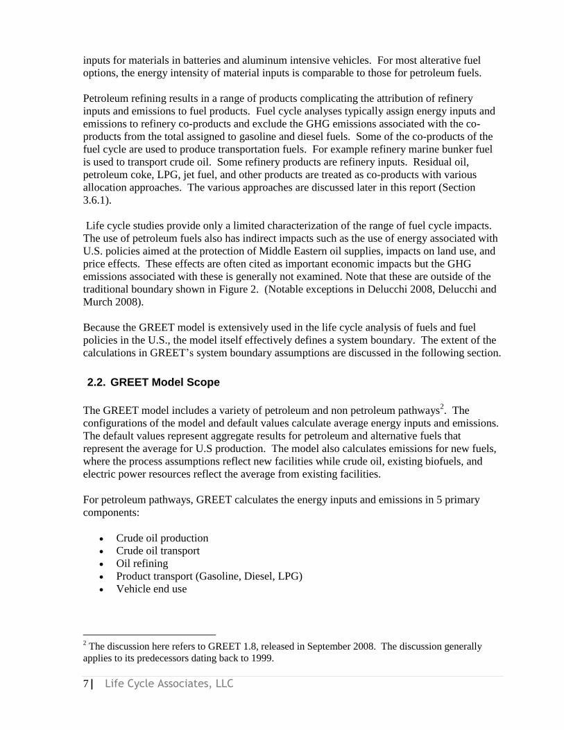
inputs for materials in batteries and aluminum intensive vehicles. For most alterative fuel
options, the energy intensity of material inputs is comparable to those for petroleum fuels.
Petroleum refining results in a range of products complicating the attribution of refinery
inputs and emissions to fuel products. Fuel cycle analyses typically assign energy inputs and
emissions to refinery co-products and exclude the GHG emissions associated with the co-
products from the total assigned to gasoline and diesel fuels. Some of the co-products of the
fuel cycle are used to produce transportation fuels. For example refinery marine bunker fuel
is used to transport crude oil. Some refinery products are refinery inputs. Residual oil,
petroleum coke, LPG, jet fuel, and other products are treated as co-products with various
allocation approaches. The various approaches are discussed later in this report (Section
3.6.1).
Life cycle studies provide only a limited characterization of the range of fuel cycle impacts.
The use of petroleum fuels also has indirect impacts such as the use of energy associated with
U.S. policies aimed at the protection of Middle Eastern oil supplies, impacts on land use, and
price effects. These effects are often cited as important economic impacts but the GHG
emissions associated with these is generally not examined. Note that these are outside of the
traditional boundary shown in Figure 2. (Notable exceptions in Delucchi 2008, Delucchi and
Murch 2008).
Because the GREET model is extensively used in the life cycle analysis of fuels and fuel
policies in the U.S., the model itself effectively defines a system boundary. The extent of the
calculations in GREET‘s system boundary assumptions are discussed in the following section.
2.2. GREET Model Scope
The GREET model includes a variety of petroleum and non petroleum pathways2. The
configurations of the model and default values calculate average energy inputs and emissions.
The default values represent aggregate results for petroleum and alternative fuels that
represent the average for U.S production. The model also calculates emissions for new fuels,
where the process assumptions reflect new facilities while crude oil, existing biofuels, and
electric power resources reflect the average from existing facilities.
For petroleum pathways, GREET calculates the energy inputs and emissions in 5 primary
components:
Crude oil production
Crude oil transport
Oil refining
Product transport (Gasoline, Diesel, LPG)
Vehicle end use
2 The discussion here refers to GREET 1.8, released in September 2008. The discussion generally
applies to its predecessors dating back to 1999.
8| Life Cycle Associates, LLC
The first four components are calculated and presented on a WTT basis with GHG emissions
in g/mmBtu. The vehicle end use phase is calculated on a WTW basis and presented in g/mi.
This phase includes the carbon in the vehicle fuel as CO2. VOC and CO are counted as CO2
with no double counting of carbon. Methane from vehicle exhaust and N2O are treated as
GHG emissions according to their global warming potential.
Many of the inputs allow for the calculation of emissions to a great degree of precision. For
example fuel spills from vehicle fuelling (0.5 g out of 8 gallons of vehicle fuelling)
correspond to 0.002 g/MJ of GHG emissions. This model feature is useful because it allows
for an understanding of the relative contribution of different fuel species. While hydrocarbons
from spills are relatively minor GHG sources, they represent a significant portion of total
hydrocarbon emissions. The great precision applied to many aspects of the calculations
implies that the GHG emissions are well established, even when some inputs exhibit
considerable variability.
The underlying assumption in GREET is that new oil, electricity, and other energy resources
will consist of a comparable resource mix as existing resources. Default GREET inputs and
the overall model structure do not reflect marginal fuel production or the impact of new fuels
and savings in fuel usage.
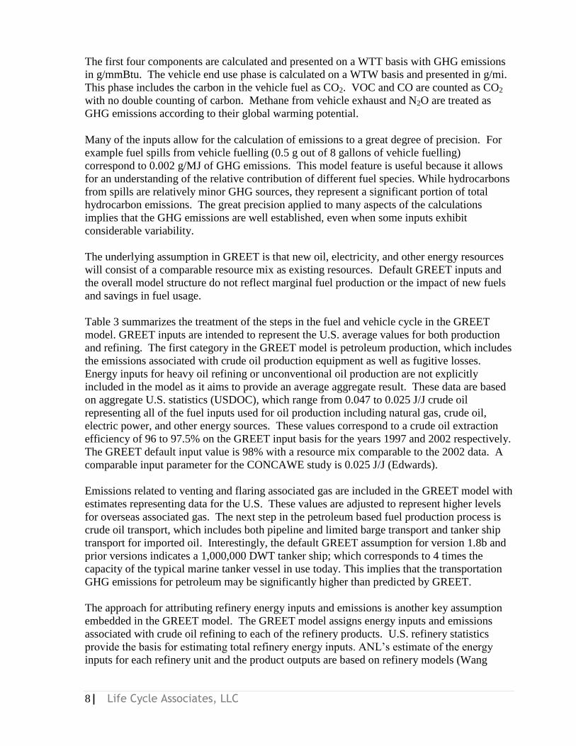
Table 3 summarizes the treatment of the steps in the fuel and vehicle cycle in the GREET
model. GREET inputs are intended to represent the U.S. average values for both production
and refining. The first category in the GREET model is petroleum production, which includes
the emissions associated with crude oil production equipment as well as fugitive losses.
Energy inputs for heavy oil refining or unconventional oil production are not explicitly
included in the model as it aims to provide an average aggregate result. These data are based
on aggregate U.S. statistics (USDOC), which range from 0.047 to 0.025 J/J crude oil
representing all of the fuel inputs used for oil production including natural gas, crude oil,
electric power, and other energy sources. These values correspond to a crude oil extraction
efficiency of 96 to 97.5% on the GREET input basis for the years 1997 and 2002 respectively.
The GREET default input value is 98% with a resource mix comparable to the 2002 data. A
comparable input parameter for the CONCAWE study is 0.025 J/J (Edwards).
Emissions related to venting and flaring associated gas are included in the GREET model with
estimates representing data for the U.S. These values are adjusted to represent higher levels
for overseas associated gas. The next step in the petroleum based fuel production process is
crude oil transport, which includes both pipeline and limited barge transport and tanker ship
transport for imported oil. Interestingly, the default GREET assumption for version 1.8b and
prior versions indicates a 1,000,000 DWT tanker ship; which corresponds to 4 times the
capacity of the typical marine tanker vessel in use today. This implies that the transportation
GHG emissions for petroleum may be significantly higher than predicted by GREET.
The approach for attributing refinery energy inputs and emissions is another key assumption
embedded in the GREET model. The GREET model assigns energy inputs and emissions
associated with crude oil refining to each of the refinery products. U.S. refinery statistics
provide the basis for estimating total refinery energy inputs. ANL‘s estimate of the energy
inputs for each refinery unit and the product outputs are based on refinery models (Wang

9| Life Cycle Associates, LLC
2004) and provide the basis for allocating energy inputs among refinery products. The
procedure treats transportation fuels and heavy oil co-products in the same manner, assigning
refinery energy and emissions to their production. These estimates are adjusted with more
recent EIA data for refinery energy (Wang 2008). The refinery energy inputs for each product
(gasoline blend stock, LPG, diesel) are represented as a ―refinery efficiency‖ value for each
product. This approach eliminates the complexity associated with tracking the fate of
different co-products. Several other approaches to the treatment of refinery energy have been
implemented in life cycle studies. These are discussed in Section 4.1.
The ―refinery efficiency‖ input assigns energy inputs to gasoline, diesel and LPG production.
The analysis does not directly take into account the fate of co-product coke and residual oil
that is produced when additional crude oil is processed. This is the case even though the coke
and residual oil are substantial outputs within the refining cycle. The model calculates
feedstock energy losses in refining processes separately from feedstock converted to fuel with
the notion that 1 million Btu of feedstock is required to produce 1 million Btu of fuel product.
The implications are discussed in Section 3.6.
Several emission sources are excluded because they represent a small fraction of the fuel
cycle. For example, chemical inputs that are consumed in small quantities or replaced during
maintenance such as catalysts are not included in GREET. Material inputs for facilities are
not included in the model as a matter of system boundary definition. ANL also calculates
some material energy inputs (for farming equipment) and demonstrates that the impacts are
small. Thus, the GREET analysis does not further calculate material inputs for the
comparison of fuel options because these emissions are a relatively small fraction of the fuel
cycle.
GREET 2.7 calculates vehicle material inputs and emissions (Burnham). These emissions
would be almost identical among comparable liquid fueled vehicles. The range in crude oil
production emissions are represented by a stochastic simulation of uncertainty. The model or
documentation does not explicitly identify data that are associated with the uncertainty
analysis parameters available in the stochastic simulation.
10| Life Cycle Associates, LLC
Table 3. Treatment of Fuel Cycle Categories for Petroleum Pathways in the GREET Model.
Category Treatment in
GREET
Comments
Facility Materials Not included Small component of fuel cycle.
Exploration and Drilling Not included Assumed to be small.
Venting and Flaring Included in crude
oil production
Data for U.S. adjusted to reflect
composite value of domestic
production and imports.
Crude Oil Production 98% crude oil
extraction efficiency
assumption applied
to feedstock
Based on aggregate U.S. statistics
(USADC). Crude oil extraction
emissions are inconsistently applied
to downstream energy inputs.
Refining Allocation to
refinery products
Refinery energy inputs based on
aggregate EIA statistics for the U.S.
Allocation to gasoline is based on
experience with refinery models
with estimate of process specific
allocation to gasoline. Inputs do not
demonstrate a material balance.
Refining Co-products Allocation to co-
products
Upstream fuel cycle emissions are
implicitly allocated to co-products
as inputs to GREET. The selection
of ―refining efficiency‖ reflects the
distribution of refinery emissions to
transportation fuels.
Chemical Inputs Not included Small component of fuel cycle.
Fuel Cycle Calculations Sum of WTT
impacts 1 mm Btu of Crude oil ―feed‖ loss
factor +
Refinery energy + distribution
Vehicle emissions TTW calculation Fuel carbon + vehicle N2O and CH4
shown on a per mile basis.
Vehicle manufacturing GREET 2.7 analysis Calculates material inputs and
recycling for vehicles. Results are
very similar for conventional
vehicles and identical for blends.
Indirect, Market-Mediated
Impacts
None GREET applies a market factor to
reduce the amount of credit applied
to corn DDGS from corn ethanol by
15%. No other market impacts are
included in GREET.
The indirect impacts of petroleum production including economic effects, land use, and
government policies associated with oil production are not included in the GREET model.
11| Life Cycle Associates, LLC
2.3. Marginal Impacts
The energy inputs and emissions associated with the production of the nth gallon of fuel
represent the impact of a change in transportation fuel usage. Changes in petroleum usage
could be due to a displacement by alternative fuels, improvements in fuel economy or a
change in consumption behavior. In principle, the highest cost producers provide the
marginal gallon of fuel. Cost factors include transport distance, tariffs, fuel specifications, as
well as well as inputs to crude oil extraction and refining. The marginal argument is often
applied to criteria pollutant emissions from new fuel production facilities in California (CEC
2005, Unnasch 2001) where a growth in alternative transportation fuels was projected to
displace gasoline imports. However, the effect on global gasoline production is less clear.
One of the reasons that it is important to consider the marginal impact of petroleum – or the
impacts of the marginal gallon of petroleum – is to ensure that fuels are compared equitably
with regard to their carbon intensity scores. For example, as discussed, recent analyses of the
life cycle impacts of biofuels have expanded the LCA system boundaries to include the price-
induced, indirect effects of ethanol production, such as LUC, based on future ethanol demand
measured in the world economy (i.e. the nth gallon of ethanol).
If the comparison is to petroleum, it is important to consider the impact of a marginal gallon
of petroleum use. Comparing marginal alternatives to average petroleum understates the
potential GHG impact.
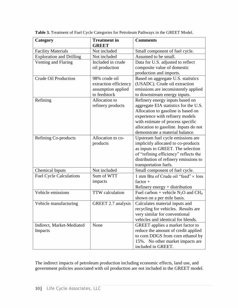
A simple model of reduced gasoline demand would be to assign the reduction in output from
the highest cost producer as illustrated in Figure 2. Displaced petroleum corresponds to the
highest cost producer. Absent this petroleum production, the crude oil would remain
underground. In practice the source of the crude oil depends on factors such as OPEC
production limits, transportation costs, national energy policies, and other factors.
Business as
Usual
Alternative
Scenario
Leave
Petroleum
Underground
To
tal E
mis
sio
ns
Reference System
Marginal Impact
Low Cost Producers
Highest
Cost
Figure 2. Life cycle impacts occur on the margin as shown by ‗business as usual‘.

12| Life Cycle Associates, LLC
Other analysis techniques could interpret the sources of marginal petroleum. These might
include:
Interviews with traders and market participants to assess capacity limitations and
supply patterns
Oil industry sector models which include supply curves based on extraction and
production technology
Consideration of capacity limits on U.S. refineries and requirements for imports of
finished product
Econometric models that estimate the effect on the U.S. and worldwide economy
based on inputs such as the production of competing fuels or fuel economy
Of course considering a broader range of factors in the life cycle of petroleum adds to the
complexity and uncertainty of the analysis. Delucchi takes the marginal argument one step
further by proposing that all life cycles of fuels should be based on a consequential analysis of
their production including the effects on resources and global prices (Delucchi 2008).
In principal, a consequential assessment of a product would determine the marginal energy
inputs and related emissions that are the result of production and use of the product. These
impacts could include activities far removed from the direct effects. For example the
consequential use of natural gas as a process fuel would include the energy required to make
up for natural gas consumed from the local gas grid. The source of energy could include:
More natural gas from existing sources
Natural gas from LNG
Reductions in natural gas demand due to price effects
Switching from natural gas to other fuels due to price effects
All other indirect and induced price effects that are the result of an increase in natural
gas usage including all factors of production in the economy
Marginal petroleum resources correspond to the more expensive and harder to reach barrel of
oil. At higher price levels more energy intensive and expensive resources such as heavy oil
and stripper wells are brought into production. Some of the sources described in this study
would certainly be considered on the margin.
2.4. Economic Effects
Economics ultimately determine which petroleum resources are produced on the margin
including factors such as production costs, sunk capital, and others. The effect of petroleum
production, consumption, and co-products also generates economic effects with resultant
GHG emissions. The factors of production associated with petroleum supply and
consumption affect the consumption of consumer goods, prices in the economy, and a
cascading effect of energy use and emissions. Price effects are largely understood to be the
response of the marketplace to a change in supply of goods.
In a theoretically perfect economy, all factors of production respond to the equilibrium of
supply and demand. The entire global economy should respond to a change in the supply of a
13| Life Cycle Associates, LLC
product such as corn or residual oil. World prices should change in response to supply
availability affecting all factors of production and economic sectors.
2.4.1. Indirect Impacts of Biofuels and Effect on Indirect Petroleum Effects
The indirect effects of biofuel production and use have been incorporated into recent life cycle
calculations. Most notably, the effects on land carbon accretion as well as a limited set of
other indirect effects of using corn as feedstock for ethanol are part of the RFS and LCFS
calculations (EPA; ARB LCFS 2009).
Direct LUC emissions are associated with the clearing of land and land preparation to grow
crops for biofuel production and include changes in soil carbon and above ground flora. All of
the above ground carbon and a significant fraction of soil carbon are converted to CO2 when
land is converted to agricultural production. The second category, indirect or market-
mediated LUC, occurs when the production of biofuels displaces some other land use (e.g.
grazing for livestock). These effects are extremely difficult to predict or measure with any
accuracy, and are highly uncertain due to their indiscriminate and often indiscreet variables.
Indirect LUC has been treated as an economic phenomenon predicted by economic (partial or
general) equilibrium models that represent food, fuel, feed, fiber, and livestock markets and
their numerous interactions and feedbacks. Results from large-scale economic models,
however, depend on a wide range of exogenous variables, such as growth rates, exchange
rates, tax policies, and subsidies for dozens of countries.
Indirect land use effects are part of the statutory requirements of the Energy Independence and
Security Act (EISA 2007). EPA is currently using the FASOM and FAPRI models to
estimate the impact from changes in crop acreage on domestic and international land use. The
GTAP model is being used by UC Berkeley and Purdue University to evaluate indirect land
use conversion impacts of biofuel production expansion. This effort is used in support of the
California LCFS.
While the assessments of LUC for biofuels provide considerable insight into the land use
impacts of fuels, these modeling efforts to date have not included all impacts that are directly
related to the use of biofuels and include:
Agricultural inputs associated with indirect crop production (example is given below)
Direct GHG emissions associated with changes in agricultural commodity transport
Broad range of consequential economic impacts
Other indirect effects are also difficult to predict and include:
Non equilibrium prices (in other words: the real world price of goods)
Effects on petroleum prices
Shifts in currently markets
Innovation-based yield and efficiency increases
Demographic trends

14| Life Cycle Associates, LLC
2.4.2. Direct and Indirect Effects of Petroleum Production
A working definition of direct and indirect effects of petroleum production produced the
groupings in Table 4 of indirect vs. direct effects and depict which are covered in more
traditional LCAs and which effects are not (as denoted by the closed vs. open circles).
Table 4. Categorization of direct vs. indirect effects of petroleum production.
Petroleum
Supply Option
Direct Effects Indirect Effects O
il E
xp
lora
tion
Oil
Pro
du
ctio
n
Met
han
e lo
sses
, fl
ari
ng
Oil
Ref
inin
g
Oil
an
d P
rod
uct
Tra
nsp
ort
Lan
d U
se C
on
ver
sion
Tail
ing l
ak
es, C
H4
Veh
icle
fu
el
Exh
au
st m
inor
spec
ies
Mate
rial
inp
uts
Ref
iner
y C
o-p
rod
uct
s
Macr
o E
con
om
ic E
ffec
ts
Pro
tect
ion
of
oil
su
pp
ly
Iraq
Rec
on
stru
ctio
n
Ind
irec
t la
nd
Use
b
Venezuelan
Heavy −
Canadian Oil
Sands − −
Iraqi − − − −
Nigerian − − − − −
California
TEOR
−
−
−
U.S. Off Shore − − − − −
Conventional − − − −
Included in traditionala fuel life cycle analysis
Excluded from traditional fuel life cycle analysis because relative difference among
fuels is small
Not included in traditional full fuel life cycle analyses
Include in traditional fuel life cycle analyses and needs much work
− Not applicable a Delucchi‘s work on fuel life cycle analysis includes many of the effects in this table or
recommends work in these areas b Market effects of petroleum would also include induced effects on land use.
15| Life Cycle Associates, LLC
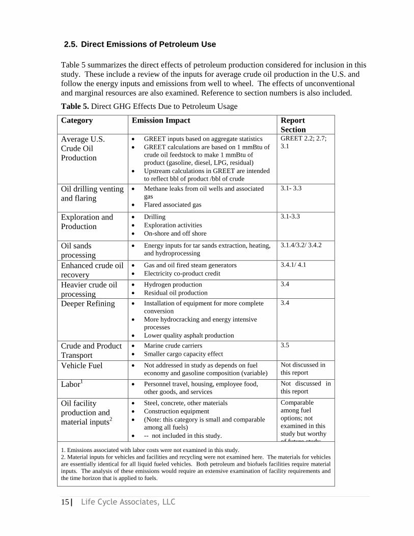
2.5. Direct Emissions of Petroleum Use
Table 5 summarizes the direct effects of petroleum production considered for inclusion in this
study. These include a review of the inputs for average crude oil production in the U.S. and
follow the energy inputs and emissions from well to wheel. The effects of unconventional
and marginal resources are also examined. Reference to section numbers is also included.
Table 5. Direct GHG Effects Due to Petroleum Usage
Category Emission Impact Report
Section
Average U.S.
Crude Oil
Production
GREET inputs based on aggregate statistics
GREET calculations are based on 1 mmBtu of
crude oil feedstock to make 1 mmBtu of
product (gasoline, diesel, LPG, residual)
Upstream calculations in GREET are intended
to reflect bbl of product /bbl of crude
GREET 2.2; 2.7;
3.1
Oil drilling venting
and flaring
Methane leaks from oil wells and associated
gas
Flared associated gas
3.1- 3.3
Exploration and
Production
Drilling
Exploration activities
On-shore and off shore
3.1-3.3
Oil sands
processing
Energy inputs for tar sands extraction, heating,
and hydroprocessing
3.1.4/3.2/ 3.4.2
Enhanced crude oil
recovery
Gas and oil fired steam generators
Electricity co-product credit
3.4.1/ 4.1
Heavier crude oil
processing
Hydrogen production
Residual oil production
3.4
Deeper Refining Installation of equipment for more complete
conversion
More hydrocracking and energy intensive
processes
Lower quality asphalt production
3.4
Crude and Product
Transport
Marine crude carriers
Smaller cargo capacity effect
3.5
Vehicle Fuel Not addressed in study as depends on fuel
economy and gasoline composition (variable)
Not discussed in
this report
Labor1 Personnel travel, housing, employee food,
other goods, and services
Not discussed in
this report
Oil facility
production and
material inputs2
Steel, concrete, other materials
Construction equipment
(Note: this category is small and comparable
among all fuels)
-- not included in this study.
Comparable
among fuel
options; not
examined in this
study but worthy
of future study.
1. Emissions associated with labor costs were not examined in this study.
2. Material inputs for vehicles and facilities and recycling were not examined here. The materials for vehicles
are essentially identical for all liquid fueled vehicles. Both petroleum and biofuels facilities require material
inputs. The analysis of these emissions would require an extensive examination of facility requirements and
the time horizon that is applied to fuels.

16| Life Cycle Associates, LLC
Indirect Effects of Petroleum Use
The indirect GHG effects of petroleum use that are outside the scope of the GREET model,
include the following high-level categories and are listed in Table 6:
1. Protection of supply
2. Land use and other environmental impacts
3. Market-mediated impacts relating to dependence on, or the price of oil3
Table 6. Potential Indirect GHG Effects Due to Petroleum Usage.
Category Emission Impact Report Section
Refinery residual oil
production Refining crude oil produces more residual
oil on the market
4.1
Protection of supply Section 4.3
Emissions from U.S.
government military
activities in defense of
Middle East oil fields
Gulf War I and II
Naval activity in Persian Gulf
Iraq occupation
Other military activities to be identified
from DOE studies
Troop training and preparation
Estimate based on $ expenditures
4.3
Increased material use (i.e.
cement) for war zone
reconstruction
Power plant, building, bridge, road
construction
War zone transport of materials
4.4.1
Oil field fires due to
military activities Kuwaiti oil fields burned for several
weeks after Gulf War I
4.4.2
Land Use Impacts Section 5.0
Tar sands and oil
production land impact
Mining, hydrogen production (in
GREET)
Disrupted carbon storage from land
Earth moving equipment to restore land
5.2
Road construction Road building is catalyst to deforestation
destruction
5.1
Economic Impacts Section 4.2
Tar sands use of natural
gas for processing Pressure on natural gas for power
production, shift to more coal imports
4.2
Price pressures on
agricultural commodities
from petroleum prices
Fertilizer, labor, seed, fuel, etc.
Shift from natural gas to coal based
fertilizers
Destruction of forest for fuel
4.2
Price pressures on
gasoline with
decreased/increased
biofuels supply
Rebound effect
4.2.2
3 The supply and demand of goods and services respond to the price of oil, thereby inducing economic effects.
The economic activities that either depend on petroleum fuels are or otherwise track the price of petroleum
would most likely also encounter changes in economic activity and resultant GHG emissions. Agricultural
commodities, travel, industrial chemicals, and a variety of goods and services are affected by petroleum prices.
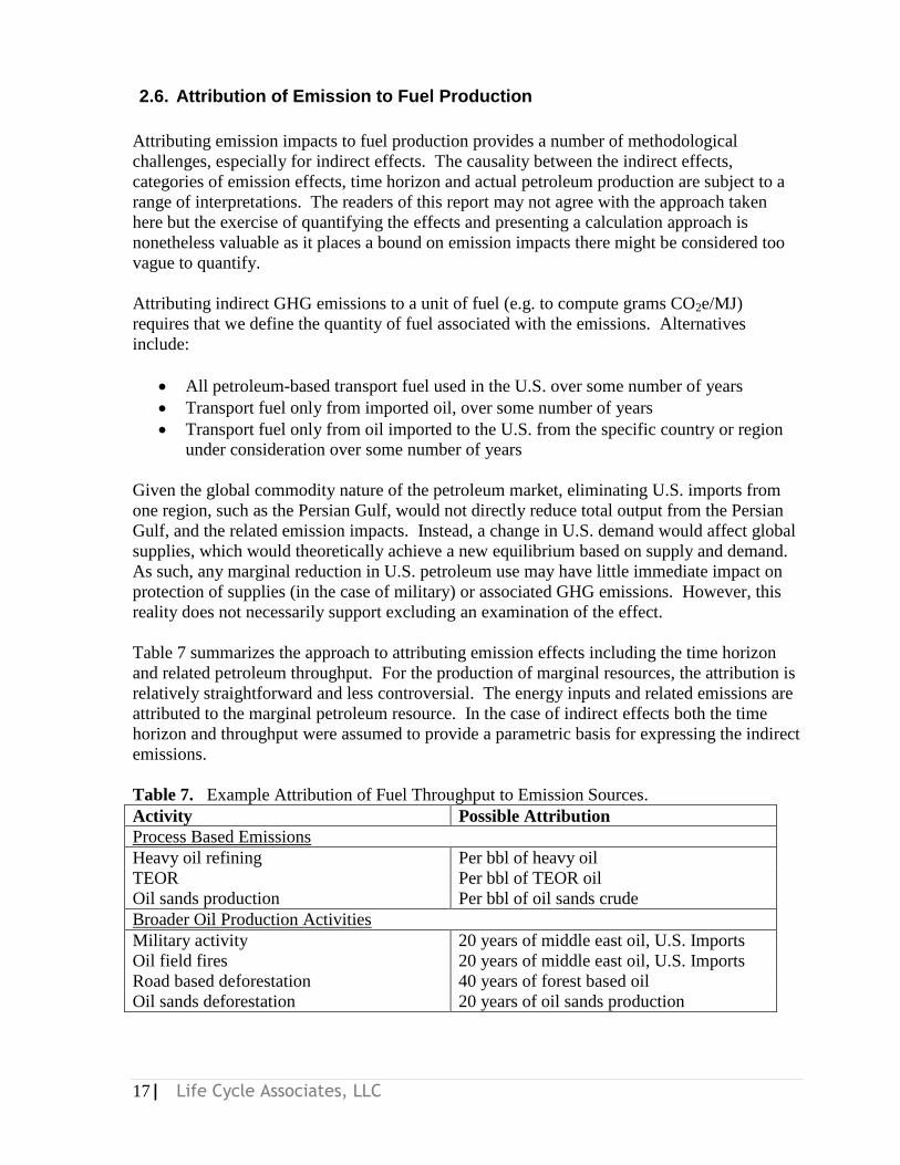
17| Life Cycle Associates, LLC
2.6. Attribution of Emission to Fuel Production
Attributing emission impacts to fuel production provides a number of methodological
challenges, especially for indirect effects. The causality between the indirect effects,
categories of emission effects, time horizon and actual petroleum production are subject to a
range of interpretations. The readers of this report may not agree with the approach taken
here but the exercise of quantifying the effects and presenting a calculation approach is
nonetheless valuable as it places a bound on emission impacts there might be considered too
vague to quantify.
Attributing indirect GHG emissions to a unit of fuel (e.g. to compute grams CO2e/MJ)
requires that we define the quantity of fuel associated with the emissions. Alternatives
include:
All petroleum-based transport fuel used in the U.S. over some number of years
Transport fuel only from imported oil, over some number of years
Transport fuel only from oil imported to the U.S. from the specific country or region
under consideration over some number of years
Given the global commodity nature of the petroleum market, eliminating U.S. imports from
one region, such as the Persian Gulf, would not directly reduce total output from the Persian
Gulf, and the related emission impacts. Instead, a change in U.S. demand would affect global
supplies, which would theoretically achieve a new equilibrium based on supply and demand.
As such, any marginal reduction in U.S. petroleum use may have little immediate impact on
protection of supplies (in the case of military) or associated GHG emissions. However, this
reality does not necessarily support excluding an examination of the effect.
Table 7 summarizes the approach to attributing emission effects including the time horizon
and related petroleum throughput. For the production of marginal resources, the attribution is
relatively straightforward and less controversial. The energy inputs and related emissions are
attributed to the marginal petroleum resource. In the case of indirect effects both the time
horizon and throughput were assumed to provide a parametric basis for expressing the indirect
emissions.
Table 7. Example Attribution of Fuel Throughput to Emission Sources.
Activity Possible Attribution
Process Based Emissions
Heavy oil refining Per bbl of heavy oil
TEOR Per bbl of TEOR oil
Oil sands production Per bbl of oil sands crude
Broader Oil Production Activities
Military activity 20 years of middle east oil, U.S. Imports
Oil field fires 20 years of middle east oil, U.S. Imports
Road based deforestation 40 years of forest based oil
Oil sands deforestation 20 years of oil sands production

18| Life Cycle Associates, LLC
Studies on military impacts generally consider the attribution question. Different approaches
described in Section 1.1 provide estimates of GHG emissions associated with supply
protection. We must then allocate these emissions to a quantity of fuel to provide a term with
the desired units of g CO2e/MJ.
For protection of petroleum supply, we consider two possible fuel quantities: (a) all transport
fuel consumed in the U.S., and (b) all transport fuel produced from oil imported from the
Persian Gulf. Table 8 shows U.S. production, imports, and exports of petroleum for the years
2003-2007.
Table 8. Total U.S. Petroleum and Transport Fuel Consumption, 2003-2007.
Category Billion bbl
Production 9.67
Imports 18.26
Persian Gulf imports 4.13
Gulf imports for transport 2.89
Exports 0.04
Net consumption 27.89
Net consumption for transport 19.52
In the past five years (2003-2007), the U.S. imported 4.1 billion barrels of crude oil from the
Persian Gulf, out of a total 18.3 billion barrels imported. Since Persian Gulf imports in this
period accounted for 15% of total U.S. consumption, the use of the smaller denominator
(Persian Gulf imports only as opposed to all imports) increases the ―supply protection adder‖
by a factor of 1/0.15 or 6.7.
An argument can be made that the protection of Persian Gulf oil serves to control the price of
all petroleum, not only in the U.S., but in the world. Since oil is a globally traded commodity,
the loss of supply anywhere causes the price to rise globally.
Copulos (Copulos 2003) writes:
―Why do military threats to the Persian Gulf warrant a military response
while threats to other regions do not? One answer is that the magnitude of
the Gulf’s production and reserves make it uniquely important. Because of
this fundamental fact, while losses from other oil producing areas can readily
be offset by surge production from the Gulf, the loss of production from the
Gulf could not be made up by surge production in other regions.‖
Copulos‘ argument that a loss of production from the Gulf would fundamentally alter the
global oil market supports the notion that ongoing military activities are effectively tied to its
oil supply. Further, Copulos‘ (2006) indicates that 50 to75 percent of Middle East military
activity is an ongoing requirement to maintain production capacity4. The calculations in
Section 3.8 assign all of the military activity to the transportation fuels derived from crude oil.
4 Included in Milton A. Copulos‘ testimony on the ‗Hidden Cost of Oil‘-to the United States
Committee on Foreign Relations: 2006.

19| Life Cycle Associates, LLC
3. Direct Petroleum Production Emissions
3.1. Exploration, Drilling, and Production
Oil production is typically the first step in a life cycle analysis of petroleum fuels. Oil
production covers a range of technologies depending on the reservoir type, extraction
technology, and oil field equipment. In addition, oil production also requires exploration to
find the oil, which is typically not included in life cycle analyses. This section examines the
data on oil exploration, drilling, and production.
3.1.1. Conventional Oil Exploration, Drilling, and Production Data
Over the years, oil production has involved progressively more intensive exploration, drilling,
and collection activities. Early oil production activities involved identifying oil seeps and
drilling relatively shallow wells. Today‘s oil exploration activities include sophisticated
seismic technologies that detect underground (and in deep water) geological formations.
Accessing the oil has also become more difficult. For example: Chevron, Devon, and Statoil
recently announced a very large oil discovery in the Gulf of Mexico, which could increase
U.S. proven reserves of oil by as much as 50%. However, exploring this source of oil would
involve drilling 20,000 feet deep (under 7,000 ft of water).
Ideally, data on energy and materials consumed in drilling would be gathered by surveying oil
and gas drilling companies. Since such data are not widely available, aggregated data, such as
from the Economic Census, provide the data for oil extraction in GREET and some other fuel
cycle analyses. In addition to the data on oil and gas extraction from the Economic Census
that was used in GREET, there is newer data presented in a document entitled Crude
Petroleum and Natural Gas Extraction, and there are two other relevant datasets generated by
the Economic Census: Oil and gas well drilling and Support activities for oil and gas
operations.
Data from the 1997 Economic Census provides additional information on oil exploration
activities as data from the 2002 Census is incomplete (USADC 1999; USADC 1999; USADC
1999). The three datasets compiled by the Economic Census are described below in Table 9.
Table 9. Economic Census Datasets.
Document Year Included activities in document
Drilling oil and
gas wells 1997
Drilling oil, gas, service wells; oil and gas well drilling
directional control; reworking oil and gas wells.
Support activities
for oil and gas
operations
1997
Exploration, geophysical exploration; Cementing; Surveying
and well logging; Running and pulling casing and rods;
Acidizing and chemical treatment; Perforating casing;
Installing equipment; Cleaning, bailing, and swabbing wells.
Crude petroleum
and natural gas
extraction
1997 Extraction of crude petroleum including lease condensate;
Extraction of gas; Extraction of unspecified hydrocarbons.
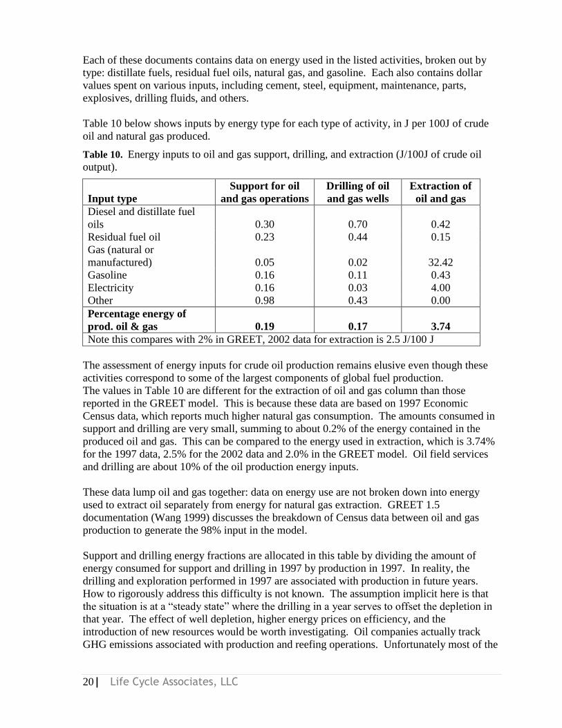
20| Life Cycle Associates, LLC
Each of these documents contains data on energy used in the listed activities, broken out by
type: distillate fuels, residual fuel oils, natural gas, and gasoline. Each also contains dollar
values spent on various inputs, including cement, steel, equipment, maintenance, parts,
explosives, drilling fluids, and others.
Table 10 below shows inputs by energy type for each type of activity, in J per 100J of crude
oil and natural gas produced.
Table 10. Energy inputs to oil and gas support, drilling, and extraction (J/100J of crude oil
output).
Input type
Support for oil
and gas operations
Drilling of oil
and gas wells
Extraction of
oil and gas
Diesel and distillate fuel
oils 0.30 0.70 0.42
Residual fuel oil 0.23 0.44 0.15
Gas (natural or
manufactured) 0.05 0.02 32.42
Gasoline 0.16 0.11 0.43
Electricity 0.16 0.03 4.00
Other 0.98 0.43 0.00
Percentage energy of
prod. oil & gas 0.19 0.17 3.74
Note this compares with 2% in GREET, 2002 data for extraction is 2.5 J/100 J
The assessment of energy inputs for crude oil production remains elusive even though these
activities correspond to some of the largest components of global fuel production.
The values in Table 10 are different for the extraction of oil and gas column than those
reported in the GREET model. This is because these data are based on 1997 Economic
Census data, which reports much higher natural gas consumption. The amounts consumed in
support and drilling are very small, summing to about 0.2% of the energy contained in the
produced oil and gas. This can be compared to the energy used in extraction, which is 3.74%
for the 1997 data, 2.5% for the 2002 data and 2.0% in the GREET model. Oil field services
and drilling are about 10% of the oil production energy inputs.
These data lump oil and gas together: data on energy use are not broken down into energy
used to extract oil separately from energy for natural gas extraction. GREET 1.5
documentation (Wang 1999) discusses the breakdown of Census data between oil and gas
production to generate the 98% input in the model.
Support and drilling energy fractions are allocated in this table by dividing the amount of
energy consumed for support and drilling in 1997 by production in 1997. In reality, the
drilling and exploration performed in 1997 are associated with production in future years.
How to rigorously address this difficulty is not known. The assumption implicit here is that
the situation is at a ―steady state‖ where the drilling in a year serves to offset the depletion in
that year. The effect of well depletion, higher energy prices on efficiency, and the
introduction of new resources would be worth investigating. Oil companies actually track
GHG emissions associated with production and reefing operations. Unfortunately most of the
21| Life Cycle Associates, LLC
data is proprietary to the oil companies and not presented in a manner that allows for a ready
assessment of GHG intensity tied to throughput and production technology. For example,
some data is presented as an aggregate of production and refining. The methods used to track
emissions also potentially differ from those in the GREET model and a significant effort
would be required to provide the data on a consistent basis.
The Census data provides no breakdown for the energy use tables in ―Support Activities‖
between energy used in different activities (e.g. exploration as compared to cementing).
Energy inputs associated with these activities could be calculated from cost inputs in the
census data. For example, the cost inputs for exploration, cementing, etc are reported. These
inputs could be related to the energy required to make the cement and steel providing insight
into the drilling and support activities.
Data for specific project or system designs could also be used to develop estimates of the
energy required for operating drill rigs, water separation, pumping, storage and other
equipment. Case studies in specific projects would be useful to understand the factors that
affect oil production energy inputs such as secondary production technologies (water
flooding), drill rig throughput, well depth, oil viscosity, and other factors. While such data
would not provide a representation of the average, a better understanding of the basis for the
aggregate data and ranges among production projects is needed to provide more confidence in
the inputs to petroleum life cycle analysis.
The ranges in energy inputs could be broader than the 2% of crude oil energy +2/- 1% cited in
the JEC study (Edwards) for marginal resources such as stripper wells. Stripper wells produce
less than 10 bbl per day. Despite their small output, about 80% of the 500,000 producing oil
wells in the U.S. are classified as stripper wells, which correspond to 19% of U.S. production
(NETL year). The equipment requirements, pumping energy, and transportation modes for
this oil resource should be examined in detail as these are typically the high cost producers
that operate on the margin. With depleted wells, low oil throughputs and transport volumes,
the energy inputs would certainly be larger than the average project. A priority in the area of
petroleum analysis would be to determine what fraction of stripper wells are represented by
the USADC census data.
Arguably, marginal impact best represents the impact of new fuels (Unnasch 2001).
Calculating average emissions is interesting from a historical perspective, while marginal
sources are affected by the displacement of petroleum due to conservation or the introduction
of new fuels. Heavy oil and unconventional oil represent an increasing share of the market as
the price of oil rises and increases in oil imports involve transporting fuels from remote
locations with more transportation energy inputs.
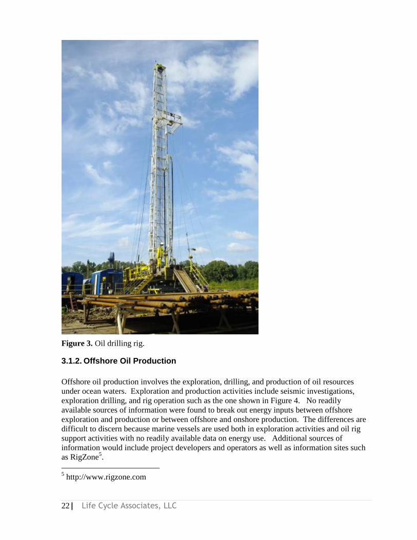
22| Life Cycle Associates, LLC
Figure 3. Oil drilling rig.
3.1.2. Offshore Oil Production
Offshore oil production involves the exploration, drilling, and production of oil resources
under ocean waters. Exploration and production activities include seismic investigations,
exploration drilling, and rig operation such as the one shown in Figure 4. No readily
available sources of information were found to break out energy inputs between offshore
exploration and production or between offshore and onshore production. The differences are
difficult to discern because marine vessels are used both in exploration activities and oil rig
support activities with no readily available data on energy use. Additional sources of
information would include project developers and operators as well as information sites such
as RigZone5.
5 http://www.rigzone.com
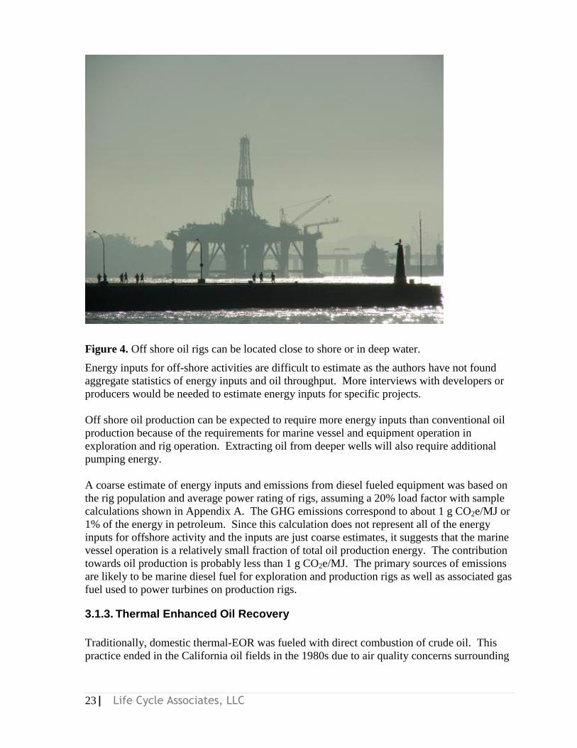
23| Life Cycle Associates, LLC
Figure 4. Off shore oil rigs can be located close to shore or in deep water.
Energy inputs for off-shore activities are difficult to estimate as the authors have not found
aggregate statistics of energy inputs and oil throughput. More interviews with developers or
producers would be needed to estimate energy inputs for specific projects.
Off shore oil production can be expected to require more energy inputs than conventional oil
production because of the requirements for marine vessel and equipment operation in
exploration and rig operation. Extracting oil from deeper wells will also require additional
pumping energy.
A coarse estimate of energy inputs and emissions from diesel fueled equipment was based on
the rig population and average power rating of rigs, assuming a 20% load factor with sample
calculations shown in Appendix A. The GHG emissions correspond to about 1 g CO2e/MJ or
1% of the energy in petroleum. Since this calculation does not represent all of the energy
inputs for offshore activity and the inputs are just coarse estimates, it suggests that the marine
vessel operation is a relatively small fraction of total oil production energy. The contribution
towards oil production is probably less than 1 g CO2e/MJ. The primary sources of emissions
are likely to be marine diesel fuel for exploration and production rigs as well as associated gas
fuel used to power turbines on production rigs.
3.1.3. Thermal Enhanced Oil Recovery
Traditionally, domestic thermal-EOR was fueled with direct combustion of crude oil. This
practice ended in the California oil fields in the 1980s due to air quality concerns surrounding

24| Life Cycle Associates, LLC
the combustion of unrefined crudes with high sulfur and metal content. California thermal-
EOR production is fueled almost entirely from natural gas.
The range of energy intensities represented by 5 historical steamflood projects is 0.21 to 0.43
MJ per MJ of incremental crude oil produced. Since these are operating steam-oil ratios,
losses in generation, steam condensation in transport lines, and heat conduction outside of the
formation are included. More recent Kern River field data illustrates the impact of accounting
for co-produced electricity (CDC-DOGGR 2007). In 2006, 92 Mbbl of water as steam was
injected into the Kern River field, approximately 73 Mbbl of which were generated in
electricity co-generation plants (CDC-DOGGR 2007). Incremental production from steam
injection was 30 Mbbl, giving a steam-oil ratio of 3.06. Steam/oil ratios in other fields were
over 5 indicating greater energy requirements for oil recovery.
The steam injection rates and fuel use from the DOGGR data allow for the calculation of
energy inputs for thermal EOR. For every MJ put into the oilfield as steam, 2 to 3.2 MJ of
natural gas was burned, but 0.5 to 1 MJ of electricity was also produced in addition to the
steam.
The steam inputs can be converted to the GREET input value of crude oil extraction
efficiency as shown in Table 11. The GWI of gasoline is calculated based on the oil
production efficiency input to GREET. In the case of CA TEOR, the fuel shares to produce
steam are set to 100% natural gas. The GWI of heavy oil with TEOR is also indicated (see
Section 3.4.2).
After taking into account a credit for electric power generation, this energy use results in
approximately 15 to 28 gCO2eq. per MJ of crude oil produced assuming natural gas is used as
the fuel, a significant increase over the 6 g CO2/MJ average value from GREET for crude oil
extraction.
The GHG emissions from TEOR are five times as high as the U.S. average calculated in
GREET. Since these emissions are calculated based on the process requirements for oil
recover rather than oil production statistics reported to the Department of Commerce, the
disparity suggests that other types of oil recover should also be examined in further detail.
However, the 15 to 28 g/MJ for TECR crude oil is not necessarily inconsistent with a U.S.
average of 6 g/MJ because thermal recovery represents less than 5% of U.S. production.
More research is necessary to explain any inconsistencies.
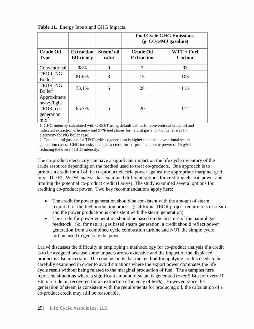
25| Life Cycle Associates, LLC
Table 11. Energy Inputs and GHG Impacts.
Fuel Cycle GHG Emissions
(g CO2e/MJ gasoline)
Crude Oil
Type
Extraction
Efficiency
Steam/ oil
ratio
Crude Oil
Extraction
WTT + Fuel
Carbon
Conventional 98% 0 7 93
TEOR, NG
Boiler1
81.6% 3 15 105
TEOR, NG
Boiler1
73.1% 5 28 113
Approximate
heavy/light
TEOR, co-
generation
mix2
65.7% 5 20 112
1. GHG intensity calculated with GREET using default values for conventional crude oil and
indicated extraction efficiency and 97% fuel shares for natural gas and 3% fuel shares for
electricity for NG boiler case.
2. Total natural gas use for TEOR with cogeneration is higher than the conventional steam
generation cases. GHG intensity includes a credit for co-product electric power of 15 g/MJ,
reducing the overall GHG intensity.
The co-product electricity can have a significant impact on the life cycle inventory of the
crude resource depending on the method used to treat co-products. One approach is to
provide a credit for all of the co-product electric power against the appropriate marginal grid
mix. The EU WTW analysis has examined different options for crediting electric power and
limiting the potential co-product credit (Larivé). The study examined several options for
crediting co-product power. Two key recommendations apply here:
The credit for power generation should be consistent with the amount of steam
required for the fuel production process (California TEOR project require lots of steam
and the power production is consistent with the steam generation)
The credit for power generation should be based on the best use of the natural gas
feedstock. So, for natural gas based steam generation, a credit should reflect power
generation from a combined cycle combustion turbine and NOT the simple cycle
turbine used to generate the power
Larivé discusses the difficulty in employing a methodology for co-product analysis if a credit
is to be assigned because some impacts are so extensive and the impact of the displaced
product is also uncertain. The conclusion is that the method for applying credits needs to be
carefully examined in order to avoid situations where the export power dominates the life
cycle result without being related to the marginal production of fuel. The examples here
represent situations where a significant amount of steam is generated (over 5 Btu for every 10
Btu of crude oil recovered for an extraction efficiency of 66%). However, since the
generation of steam is consistent with the requirements for producing oil, the calculation of a
co-product credit may still be reasonable.
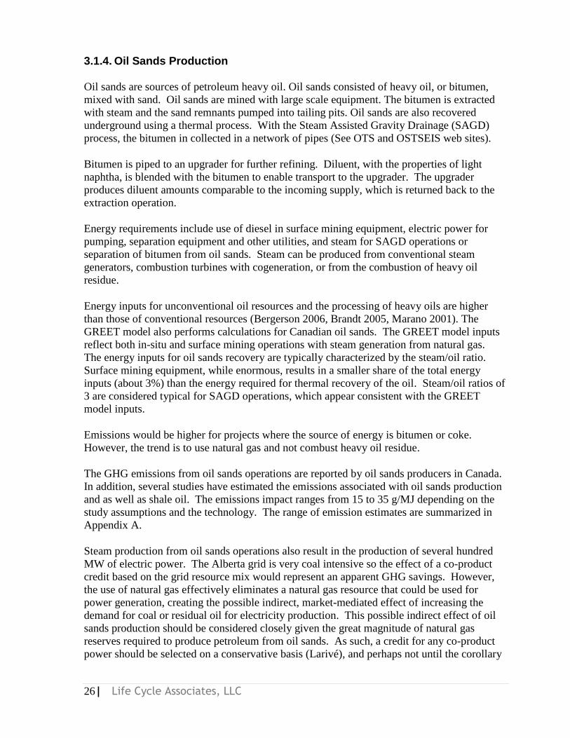
26| Life Cycle Associates, LLC
3.1.4. Oil Sands Production
Oil sands are sources of petroleum heavy oil. Oil sands consisted of heavy oil, or bitumen,
mixed with sand. Oil sands are mined with large scale equipment. The bitumen is extracted
with steam and the sand remnants pumped into tailing pits. Oil sands are also recovered
underground using a thermal process. With the Steam Assisted Gravity Drainage (SAGD)
process, the bitumen in collected in a network of pipes (See OTS and OSTSEIS web sites).
Bitumen is piped to an upgrader for further refining. Diluent, with the properties of light
naphtha, is blended with the bitumen to enable transport to the upgrader. The upgrader
produces diluent amounts comparable to the incoming supply, which is returned back to the
extraction operation.
Energy requirements include use of diesel in surface mining equipment, electric power for
pumping, separation equipment and other utilities, and steam for SAGD operations or
separation of bitumen from oil sands. Steam can be produced from conventional steam
generators, combustion turbines with cogeneration, or from the combustion of heavy oil
residue.
Energy inputs for unconventional oil resources and the processing of heavy oils are higher
than those of conventional resources (Bergerson 2006, Brandt 2005, Marano 2001). The
GREET model also performs calculations for Canadian oil sands. The GREET model inputs
reflect both in-situ and surface mining operations with steam generation from natural gas.
The energy inputs for oil sands recovery are typically characterized by the steam/oil ratio.
Surface mining equipment, while enormous, results in a smaller share of the total energy
inputs (about 3%) than the energy required for thermal recovery of the oil. Steam/oil ratios of
3 are considered typical for SAGD operations, which appear consistent with the GREET
model inputs.
Emissions would be higher for projects where the source of energy is bitumen or coke.
However, the trend is to use natural gas and not combust heavy oil residue.
The GHG emissions from oil sands operations are reported by oil sands producers in Canada.
In addition, several studies have estimated the emissions associated with oil sands production
and as well as shale oil. The emissions impact ranges from 15 to 35 g/MJ depending on the
study assumptions and the technology. The range of emission estimates are summarized in
Appendix A.
Steam production from oil sands operations also result in the production of several hundred
MW of electric power. The Alberta grid is very coal intensive so the effect of a co-product
credit based on the grid resource mix would represent an apparent GHG savings. However,
the use of natural gas effectively eliminates a natural gas resource that could be used for
power generation, creating the possible indirect, market-mediated effect of increasing the
demand for coal or residual oil for electricity production. This possible indirect effect of oil
sands production should be considered closely given the great magnitude of natural gas
reserves required to produce petroleum from oil sands. As such, a credit for any co-product
power should be selected on a conservative basis (Larivé), and perhaps not until the corollary

27| Life Cycle Associates, LLC
indirect effects analysis has been conducted. The GREET model provides no co-product
electric power credit for oil sands operations.
3.1.5. Oil Exploration and Production Recommendations
Considerable efforts have been applied to analyzing the direct emissions associated with
exploration and production of petroleum; however, many impacts of petroleum production
remain vaguely characterized. The greatest challenge is difficulty in relating data based on
surveys and statistics to specific elements of the petroleum industry. Further investigation of
the following activates would improve the understanding of petroleum fuels.
The energy inputs and emissions associated with oil production require further analysis to
provide a better understanding of the different types of petroleum supply options. GREET
model inputs rely on aggregate statistics that are difficult to validate and vary substantially
over the two reporting periods that were examined. The data inputs for other life cycle studies
are also limited. Petroleum production activities are generally lumped into one category when
there are a broad range of production options and technologies6. This lack of understanding
applies to the fuels that power almost all of our current transportation systems.
The following activities would provide a better understanding of petroleum production
emissions:
Perform an engineering analysis of the energy and GHG emissions associated with
different types of oil and oil sands operations (Note several studies are underway)
Relate oil company reported GHG emissions to life cycle inputs
Summarize the best available analysis for oil production emissions and present the
information to individual oil producers, exploration companies, and others working in
the oil production industry
3.2. Oil Sands Tailings
Residue from oil sands processing is another source of criteria pollutant and GHG emissions.
For mined operations, bitumen is separated from oil at an extraction plant which recovers
about 75% of the bitumen. The remaining bitumen/sand mixture is returned to the mine and
in some instances is stored in tailing ponds (Figure 5). The environmental impacts of these
ponds is the subject of considerable attention and results in environmental impacts other than
GHG emissions (www.oilsandswatch.com).
Methane emissions from tailing ponds and peat soils as well as land use impacts are another
potential source of GHG emissions associated with oil sands. Residual hydrocarbons from oil
extraction operations could degrade to form methane under anaerobic conditions. Tailings
ponds that occur on soils with high levels of peat may provide anaerobic conditions that
support the decomposition of peat and formation of methane. These effects are being
examined by UC Davis and the University of Calgary; thus they were not examined here.
6 GHGenius has several categories for oil production

28| Life Cycle Associates, LLC
Since the global warming potential of methane is 25 times higher than that of CO2, this
significant potential source of GHG emissions should be incorporated into the life cycle
analysis of petroleum fuels.
Figure 4. Oil sands tailing ponds are a potential source of hydrocarbon emissions. Anaerobic
conditions in peat soils could accelerate methane production.
3.3. Natural Gas Venting and Flaring
When crude oil is brought to the surface from several kilometers below, gas associated with
the oil extraction usually comes to the surface as well. If oil is produced in areas of the world
which lack gas infrastructure or a nearby gas market, a significant portion of this associated
gas may be released into the atmosphere, un-ignited (vented) or ignited (flared). Flaring of
gas either as a means of disposal or as a safety measure to relieve well pressure is the most
significant source of air emissions from oil and gas installations. Even if continuous flaring
ended, occasional burning of small amounts of gas will still be necessary for safety reasons,
such as releasing excess pressure.
According to satellite data released by the U.S. National Oceanic and Atmospheric Agency
(NOAA), in 2006 oil producing countries and companies burned about 170 billion cubic
meters (bcm) of natural gas worldwide or nearly five trillion cubic feet. That‘s equivalent to
27% of total U.S. natural gas consumption or 5.5% of total global production of natural gas
for the year. If the gas had been sold in the United States instead of being flared, the total US
market value would have been about $40 billion.
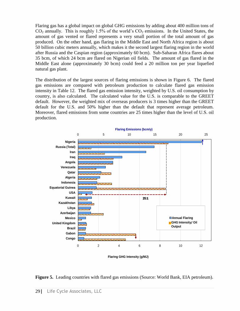
29| Life Cycle Associates, LLC
Flaring gas has a global impact on global GHG emissions by adding about 400 million tons of
CO2 annually. This is roughly 1.5% of the world‘s CO2 emissions. In the United States, the
amount of gas vented or flared represents a very small portion of the total amount of gas
produced. On the other hand, gas flaring in the Middle East and North Africa region is about
50 billion cubic meters annually, which makes it the second largest flaring region in the world
after Russia and the Caspian region (approximately 60 bcm). Sub-Saharan Africa flares about
35 bcm, of which 24 bcm are flared on Nigerian oil fields. The amount of gas flared in the
Middle East alone (approximately 30 bcm) could feed a 20 million ton per year liquefied
natural gas plant.
The distribution of the largest sources of flaring emissions is shown in Figure 6. The flared
gas emissions are compared with petroleum production to calculate flared gas emission
intensity in Table 12. The flared gas emission intensity, weighted by U.S. oil consumption by
country, is also calculated. The calculated value for the U.S. is comparable to the GREET
default. However, the weighted mix of overseas producers is 3 times higher than the GREET
default for the U.S. and 50% higher than the default that represent average petroleum.
Moreover, flared emissions from some countries are 25 times higher than the level of U.S. oil
production.
0 5 10 15 20 25
0 2 4 6 8 10 12
Congo
Gabon
Brazil
United Kingdom
Mexico
Azerbaijan
Libya
Kazakhstan
Kuwait
USA
Equatorial Guinea
Indonesia
Algeria
Qatar
Venezuela
Angola
Iraq
Iran
Russia (Total)
Nigeria
Flaring Emissions (bcm/y)
Annual Flaring
25:125:1
Flaring GHG Intensity (g/MJ)
25:1
Flaring GHG Intensity (g/MJ)
25:1
Flaring GHG Intensity (g/MJ)
25:1
Flaring GHG Intensity (g/MJ)
GHG Intensity/ Oil
Output
Figure 5. Leading countries with flared gas emissions (Source: World Bank, EIA petroleum).

30| Life Cycle Associates, LLC
Venting of natural gas is actually a larger GHG source than flared when the warming potential
of methane is taken into account. About 5 times as much methane if flared compared with
vented but the GWP for methane is 25 times higher than that of CO2 which is the end product
for most of the flared gas. Vented gas emissions would also be higher in regions outside the
U.S. GREET inputs for vented emissions are based on EIA data for vented gas in the U.S.
divided by U.S. petroleum production (Wang 1999). GREET inputs for aggregate venting
emissions are based on ANL‘s assumption that ―flared and vented gas per barrel of imported
oil is twice that associated with domestic oil production‖.
Interestingly, the aggregate flaring estimate in GREET is comparable to the value calculated
here for the Worldbank data even though the data is quite inconsistent in terms of the relative
emissions by country. Presumably a number of offsetting parameters result in the
serendipitous result. The Worldbank estimates for flaring, up to 400 million tones CO2
annually, are based on satellite observations while the EIA data for the U.S. flaring are based
on emission factors and reporting from emission sources. The wide range in flaring data
suggests that the emissions associated with natural gas venting are also large. Venting
emissions depend both on equipment and operational practices as well as the amount of
associated gas produced per barrel of oil. These data are not well reported; so, a high degree
of uncertainty should be associated with vented gas emissions.
Vented gas is also a significant source of GHG emissions and the assumption that imported
emissions are only twice U.S. levels is likely optimistic given the extensive efforts applied in
the U.S. to limit methane losses. Methane venting occurs because of a number of factors.
Gas produced with oil production leaks around casings. The extent of such leaks is a function
of the amount of gas that is produced with oil as well as the type of oil production equipment.
Associated gas may also be vented rather than flared but this practice is not safe. Examining
the operational practices of oil fields would provide more insight into venting. However,
obtaining access to such information would be challenging.
If the Worldbank data for flared gas represent the relative ratio of overseas to U.S. vented gas,
then the factors in GREET are understated and worth examining more carefully as their
estimate for CO2 emissions is equivalent to 30% of the EU‘s gas consumption
(www.worldbank.org).
3.3.1. Future Trends in Venting and Flaring
Vented and flared gas emissions are a very substantial source of GHG emissions and
international efforts are underway to address these emissions. As a first global
countermeasure, the Global Gas Flaring Reduction public-private partnership (GGFR) was
launched by a World Bank initiative in August 2002. GGFR is a collaboration of
governments, state-owned companies and major international oil companies committed to
reducing flaring and venting worldwide. The GGFR facilitates and supports national efforts
to use currently flared gas by promoting effective regulatory frameworks and tackling the
constraints on gas utilization, such as insufficient infrastructure in developing countries and
poor access to local and international energy markets, particularly in developing countries.

31| Life Cycle Associates, LLC
Table 12. Estimate of Natural Gas Flaring in Oil Producing Countries.
Country Flaring
(bcm/y)
Production
(1000 bbl/d)
U.S.
Consumption
Flared
m3/bbl
g/gal
Crude
g/MJ
Gasoli
ne
20 Congo 1.2 222 0.4% 14.8 620 4.65
19 Gabon 1.5 230 0.4% 17.9 748 5.62
18 Brazil 1.5 1833 1.0% 2.2 94 0.70
17 United Kingdom 1.6 1636 0.6% 2.7 112 0.84
16 Mexico 1.5 3477 8.3% 1.2 49 0.37
15 Azerbaijan 2.5 868 0.3% 7.9 330 2.48
14 Libya 2.5 1848 0.5% 3.7 155 1.16
13 Kazakhstan 2.7 1490 0% 5.0 208 1.56
12 Kuwait 2.7 2526 1.0% 2.9 123 0.92
11 USA 2.8 6978 40.7% 1.1 46 0.35
10 Equatorial Guinea 3.6 363 0.1% 27.2 1138 8.54
9 Indonesia 3.7 969 0.1% 10.5 438 3.29
8 Algeria 4.3 2000 2.6% 5.9 247 1.85
7 Qatar 4.5 1197 0% 10.3 431 3.24
6 Venezuela 5.4 2613 6.8% 5.7 237 1.78
5 Angola 6.8 1723 2.9% 10.8 453 3.40
4 Iraq 8.6 2145 2.9% 11.0 460 3.45
3 Iran 13.3 4401 0% 8.3 347 2.60
2 Russia (Total) 14.9 9978 0.7% 4.1 171 1.29
1 Nigeria 24.1 2356 6.4% 28.0 1173 8.81
Total 5.485 75.7% 1.58
Attribution to oil production assuming 90% of flaring is associated with oil
production.
U.S. venting emissions estimated at 43.36 g CH4/mmBtu with average of 69.54
g CH4/mmBtu as GREET default.
GREET oil processing leaks are inferred by subtracting combustion emissions
from total methane from oil production with a default calculation of 15.33 g
CH4/mmBtu
Nigerian/U.S. on a gCO2e/MJ basis = 25:1
GREET Defaults
Flaring:
Venting:
Oil processing:
0.87
1.65
0.36
32| Life Cycle Associates, LLC
As seen in Table 12 (above), the energy industry must end the flaring of natural gas and the
resulting greenhouse gas contribution. Progress has been slow so far but there are signs that
efforts to curb the practice will pay off.
In general, there are four different technical solutions for preventing gas flaring:
1. Gas re-injection in oil producing fields to enhance oil recovery or in wet gas fields to
maximize liquids recovery (Algeria)
2. Pooling of flare gas resources and construction of a LNG plant with an export terminal
(Angola, Regional solution including Equatorial Guinea, Cameroon and Nigeria)
3. Building chemical plants near oil fields to produce liquid fuels like GTL, DME, LPG
or Methanol (First pilot studies and plants)
4. Power generation with conventional gas turbines (Russia, Germany), gas engines
(Egypt) or micro-turbines
Inexpensive natural gas feedstock is vital to allow methanol, DME, and FTD to compete with
petroleum-based fuels. Production of liquid fuels from flared gas can overcome the natural
gas distribution infrastructure hurdle in remote locations; such production results in very
substantial energy and emissions benefits for produced liquid fuels because of the energy and
emission credits from eliminating gas flaring.
Fiscal incentives for reducing gas flaring are often imposed as an economic penalty and put
into law by countries making loans or guarantees given by the Worldbank. Likewise, those
countries participating in the Clean Development Mechanism (CDM) (eg. carbon credit
markets) allow for cost reductions, and therefore environmental benefits, for projects that are
verified under the CDM and then sold via the CDM‘s voluntary mechanism to countries that
wish to offset emissions.
The Nigerian Kwale Project, where flare gas is gathered and burned in a 480 MW combined
cycle power plant is an example of the Clean Development Mechanism (CDM) at work. The
objective under CDM is to offer Carbon Credits to a CO2 polluter (such as someone wishing
to offset their airmiles, or a western factory wishing to offset emissions) as a mechanism to
offset their CO2 emissions. The ultimate goal is to create an environmentally friendly
development in the developing world, such as the Kwale Project, where flaring emissions are
reduced as the CH4 and CO2 are captured (and therefore cycled into the system) and marketed
to end consumers as gas. However, a clear path needs to be identified for reducing venting
and flaring emissions before such emissions from remote locations can be considered on par
with more closely controlled production resources in the U.S. (Clean Development
Mechanism.2007).
3.3.2. Venting and Flaring Recommendations
Aggressive control of these emissions over the next twenty years might substantially reduce
overall greenhouse gas emissions. However, there have been no estimates that allow the
authors to predict how effective control of these emissions will be in the interim.

33| Life Cycle Associates, LLC
With regard to the carbon lifecycle of petroleum, the accuracy of venting emissions should be
improved by investigating emission inventories and other studies for the top oil producing
regions and relating these emissions to petroleum throughput.
3.4. Petroleum Refining
Modern oil refineries such as the one shown in Figure 6 produce a variety of fuels and other
co-products. Gasoline, diesel, and kerosene, are the primary transportation fuel products,
while LPG and residual oil are also used as fuels for heating, power generation, and transport.
Refineries also produce coke and sulfur as co-products and some refineries produce asphalt.
Attributing energy inputs to refined products is a challenging exercise complicated by the
requirements of producing different products. For example, a crude oil distillation unit
separates crude oil into different product streams to enable the refining of all refinery products
while an alkylation unit operates to produce only higher-octane components for blending into
gasoline. Several approaches have been considered for attributing refinery energy inputs and
emissions to fuel products.
Figure 6. Modern Oil Refinery.

34| Life Cycle Associates, LLC
3.4.1. Conventional Petroleum Refining
The method used to assign energy inputs to refined products is challenging because of the
complex nature of refineries. Modern oil refineries produce a variety of fuels and other co-
products. Gasoline, diesel, and kerosene, are the primary transportation fuel products, while
LPG and residual oil are also used as fuels for heating, power generation, and transport.
Refineries also produce coke and sulfur as co-products and some refineries produce asphalt.
Interestingly, some of the fuels are co-products themselves.
The method for determining ―refining efficiency‖ in GREET effectively allocates energy and
emissions to gasoline, diesel, and other products. Oil refineries produce a variety of products
using different processes within the refinery to separate product streams, remove sulfur,
convert hydrocarbons to high octane components, and many other functions.
Attributing energy inputs to refined products is a challenging exercise complicated by the
requirements of producing different products. Several approaches have been considered for
attributing refinery energy inputs and emissions to fuel products.
The simplest co-product strategy is to assign all refinery emissions and all of the combusted
energy to transportation fuel products in proportion to the energy content of the gasoline,
kerosene, and diesel produced. This is essentially the energy allocation method, applied to
transportation fuels with the understanding that residual oil and LPG are not the primary
products of the refinery, as substitutes with less energy input are readily available.
LPG is a limited transportation fuel as are aviation and marine fuels – at least in the sense that
all of these are regulated as mobile sources. This approach does not distinguish between the
energy intensity of gasoline or diesel production and more importantly, it does not allow for
an assessment of the production of different types of gasoline or diesel fuel as the refinery
impacts would be commingled between gasoline and diesel.
Several approaches could be implemented to better understand the attribution of refinery
energy inputs to fuel products. Linear programming models or a mass and energy balance
based on refinery unit performance data could provide the material balances needed to track
the feedstock, fuels, utilities, and emission sources within a refinery.
A linear programming analysis would need to take into account all of the refinery processes,
crude oil mix, and economic factors that affect refined petroleum products. A linear
programming analysis of refineries would need to be coupled with the impact on the crude oil
slate. The effect on imported product would also need to be considered. Such a
comprehensive modeling exercise aimed at assessing the impact of reducing gasoline demand
has not been undertaken. Such an approach could better relate crude oil composition to fuel
specifications, hydrogen requirements, and product yields.
The allocation approach in GREET presents a number of challenges, which tend to understate
the GHG emissions of gasoline and diesel fuels associated with refining. The core aspect of
the approach is to match EIA data on refinery energy with notional values for the relative

35| Life Cycle Associates, LLC
energy intensity for gasoline refining. The key challenges with the approach include the
following:
Input requires aggregate data. Not able to examine effect of oil type, API gravity,
sulfur, etc.
Notional gasoline energy intensity does not necessarily apply uniformly to all crude
types and refining schemes
1 mmBtu of crude oil is assigned to 1 mmBtu of gasoline
1 mmBtu of bitumen oil is assigned to 1 mmBtu of gasoline (see Roach presentation)
Fuel cycle emissions for natural gas are applied only to about one third of the natural
gas used to produce hydrogen. (No fuel cycle emissions are applied to the natural gas
feeding the hydrogen reformer). This results in a hydrogen carbon intensity that is 6 g
CO2e/MJ too low. For fuels that use significant amount of hydrogen, the carbon
intensity is under reported by 0.5 g CO2e/MJ (6 g/MJ 0.07 J H2/J product)
No fuel cycle or WTT emissions are applied to refinery fuel gas (this assumption is not
consistent with 1 mmBtu of crude oil assigned to producing 1 mmBtu of gasline). The
fuel cycle emissions associated with gasoline refining appear to be under reported by
0.5 g/MJ7
Coal content and coal WTT emissions are assumed for petroleum coke
Oil sand upgrader burns only natural gas, not fuel gas
Some of the nuances of the GREET approach may be attributed to the allocation scheme.
However, on balance, the treatment of oil refining should more closely reflect the process
units used to produce products and the impact of crude oil types. Most of the factors
identified above affect the upstream energy inputs for the refining, which results correspond
to about 10 to 16 g/MJ of GHG emissions in the refining phase. The uncertainty might be
another 2 g/MJ (plus an additional 5 to 10 g/MJ for upgrading bitumen or heavy oil). The
range in emissions is currently being investigated in several studies.
The relative impact may be small on a per MJ basis; but oil refining is the 3rd
largest source of
GHG emissions in California, behind fuel combustion and power generation. The GHG
emissions of this important industry should be better characterized. Several studies are
examining these impacts. The effect of refinery co-products is examined in Section 3.6.
3.4.2. Heavy Oil and Oil Sands Upgrading
Sources of heavy crude oil are also growing in market share. Heavy oil has a lower hydrogen
to carbon ratio than lighter oil and requires additional hydrogen to upgrade it for refining.
Also, higher levels of residual oil may be produced when heavy oil is refined.
Unconventional oils are characterized by an API gravity lower than 10 (including oil sands).
Oil with an API gravity below 18 would still be considered heavy. These oils are
characterized by a high viscosity and typically higher levels of sulfur, nitrogen, metals, and
asphaltenes. Many technology providers have developed hydrocracking processes that are
7 Total energy inputs to refinery is 1/87% or 1.15 J Energy per J Gasoline. 50% of the emissions are assigned to still gas.
Since still gas is derived from crude oil with an upstream GHG intensity of 7 to 20 g/MJ, then the upstream GHG impact of
still gas would be 0.5 0.15 J/J gasoline 7 g/MJ = 0.5 g CO2e/MJ gasoline.
36| Life Cycle Associates, LLC
suited for the conversion and upgrading of a variety of heavy oil materials ranging from
conventional vacuum residues up to extra-heavy oils and bitumen.
Upgraders can be configured with a variety of processing units including vacuum distillation,
hydro cracking, delayed coking, and hydrotreating of naphtha. Upgraders require
approximately 1000 scf of hydrogen per bbl of bitumen. The per bbl volume of upgrader
product, synthetic crude oil (SCO), depends on the technology used and ranges from 85 to 101
bbl per bbl of bitumen (Roach). Because of the presence of high density naphthenes,
aromatics and polar compounds, the H/C ratio is very low compared to the gasoline and
diesel fuel products. The increase of the H/C ratio is accomplished by rejecting carbon and
adding hydrogen. Carbon rejection processes (such as visbreaking and coking) show very
high feedstock flexibility, but generate low quality distillates and significant amounts of coke.
Hydrocracking technologies result in a higher yield with more hydrogen consumption but
these units are sensitive to feedstock quality.
Current GREET modeling for U.S. refining presumably reflects the impacts of heavy oil from
Kern County, California and Venezuela because the GREET inputs are for aggregate U.S.
refinery statistics. However, GREET inputs do not readily allow for the calculation of the
impact of heavy oil individually.
The key factors affecting the emissions from processing heavy oil are they hydrogen
consumption and the conversion yield to fuel products. Hydroprocessing equipment also
requires heating, fans, pumps, and other utilities. The impact of processing heavy oils is best
addressed by examining refinery flow sheets that are configured for light and heavy oil
configurations. Linear programming models could also be used to parametrically examine the
effect of oil properties. Such an exercise would need to examine the other impacts, such as
the refinery configuration as the LP model generally optimizes on lowest cost. The effect on
refinery units would need to be taken into account so that the modeling represents realistic
refineries. Absent a study on refining, many references identify the hydrogen requirements
for different refinery processes. The hydrogen processing chapter of the Handbook of
Petroleum Refining Processes (Meyers) identifies the hydrogen consumption for heavy oil
hydrotreating at 400 to 1000 scf/bbl oil and residuum hydrocracking at 1200 to 1600 scf/bbl.
The GHG impact of hydrogen consumption alone corresponds to 5 to over 10 g/MJ of GHG
emissions. Appendix A shows scoping calculations based on making up the hydrogen in
heavy oil to the hydrogen content in lighter oil.
3.4.3. Oil Refining Recommendations
Considerable uncertainty persists in the approach to assigning refinery energy inputs and
emissions to finished product. Aggregate statistics from EIA reflect refineries in each PADD
and allow for the calculation approach used in GREET. However, this approach does not
allow for the assessment of differences in crude oil type and composition or the evaluation of
different gasoline formulations. The approach for assessing the energy intensity of each
petroleum product is also not transparent.
Several studies are examining the effects of crude oil type on the GHG intensity of oil refining
and oil sands upgrading. These study results and others should be examined to provide a

37| Life Cycle Associates, LLC
consistent and transparent basis for attributing refinery emissions to petroleum production.
Also, the effect of refining different grades of crude oil and the impacts of co-products needs
to be reflected in the petroleum fuel cycle. Such results are expected to be available from
several studies in 2009.
3.5. Crude and Product Transport
Petroleum transport is a relatively small portion of the fuel cycle GHG emissions when
compared to the total for average processes. However, significant quantities of oil and
product are moved in smaller vessels. Oil from stripper wells may even be transported by
truck. When the crude oil and product are transported in smaller equipment, the relative GHG
emissions grow substantially. With a few exceptions, the largest marine crude carriers have a
capacity of 250,000 DWT (Figure 7). Smaller tankers are often used to transport finished
product in the event of shortages. The effect of fuel transport is illustrated in Table 13.
Table 13. Impacts of Crude Oil Transportation Mode.
Transport Impact GHG Impact
100% overseas oil
1,000,000 to 250,000 DWT oil tankera
0.17 g/MJ
50,000 DWT product tankers 1.2 g/MJ
Stripper well operation
100 mi truck transport 0.6 g/MJ aGREET default reflect 1,000,000 DWT super tanker. Most crude carriers are close to
200,000 DWT and product tankers can be even smaller.
Figure 7. Crude Oil Tanker

38| Life Cycle Associates, LLC
As noted above, the impact of fuel transportation is generally considered a small portion of
the energy inputs and emissions associates with petroleum fuels. However, higher emission
impacts occur on the margin as indicated here. The GHG emission intensity rises rapidly with
smaller cargo capacity. Also, unconventional fuel transportation practices such as storing
crude oil aboard tanker ships at sea (New York Times, January 15, 2009) also leads to higher
GHG emissions. In order to better asses these GHG impacts, a better understanding of fuel
transport practices and the inventory of crude and product carriers should be developed.
3.6. Refinery Co-Products
Oil refineries produce a variety of products using different processes within the refinery to
separate product streams, remove sulfur, convert hydrocarbons to higher octane components,
and to perform many other functions. Gasoline, diesel, and kerosene, are the primary
transportation fuel products, while LPG and residual oil are also used as fuels for heating,
power generation, and transport. Refineries also produce coke and sulfur as co-products and
some refineries produce asphalt. Interestingly, some of the fuels are co-products themselves.
In general, displacing gasoline with alternative fuels would reduce the imports of crude oil to
the U.S. and world wide refinery output and crude oil consumption. Such a shift in crude oil
consumption would result in less residual oil and petroleum coke production and the
emissions associated with the combustion of these products. The effect of reducing residual
oil and coke output would be an increase in prices and a change in consumption patterns.
Price increases could result in a reduction in consumption or a shift to other fuels such as coal,
natural gas, or renewables (for power generation). These effects are not well characterized by
life cycle models.
Arguably, the additional residual oil contributes to the supply of bunker fuel for luxury
commerce such as shipping bottled water from Fiji to the U.S. or waffles from Belgium to
England and from England to Belgium). The U.S. petroleum economy alone produces
230,000 bbl/y of residual oil and 220,000 bbl/y equivalent of coke along with 3,000,000 bbl/y
of gasoline, 540,000 bbl/y of kerosene, and 1500,000 bbl/y of diesel fuel.
Figure 8 shows the imports of petroleum products to the U.S. Most notably the U.S. is a net
importer of crude oil and an exporter of coke and residual oil. The mix of U.S. imports is also
relevant when calculating distances associated with crude oil transport indicated in Figure 9.
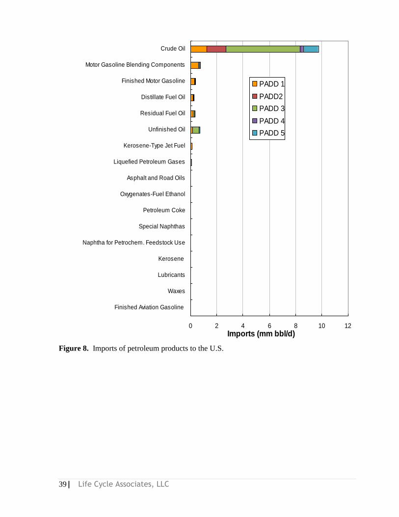
39| Life Cycle Associates, LLC
0 2 4 6 8 10 12
Finished Aviation Gasoline
Waxes
Lubricants
Kerosene
Naphtha for Petrochem. Feedstock Use
Special Naphthas
Petroleum Coke
Oxygenates-Fuel Ethanol
Asphalt and Road Oils
Liquefied Petroleum Gases
Kerosene-Type Jet Fuel
Unfinished Oil
Residual Fuel Oil
Distillate Fuel Oil
Finished Motor Gasoline
Motor Gasoline Blending Components
Crude Oil
Imports (mm bbl/d)
PADD 1
PADD2
PADD 3
PADD 4
PADD 5
Figure 8. Imports of petroleum products to the U.S.
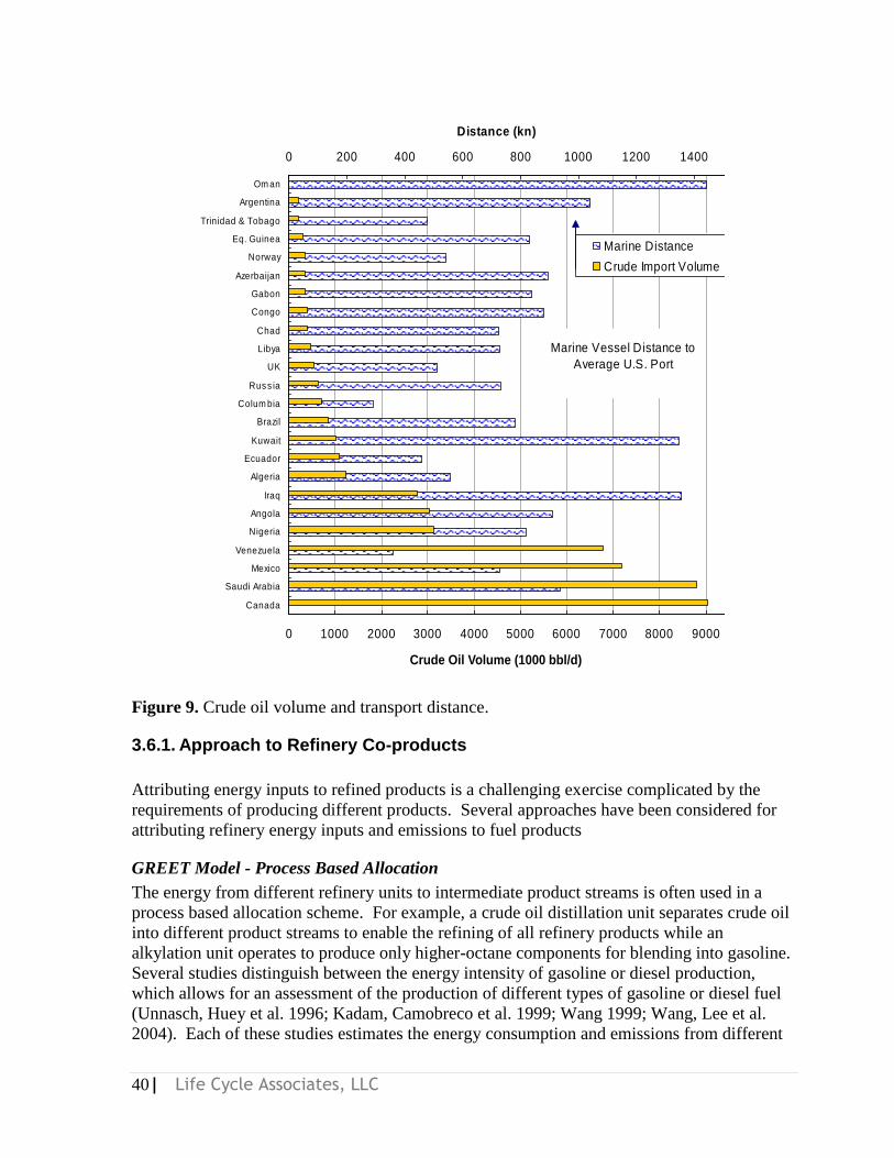
40| Life Cycle Associates, LLC
0 1000 2000 3000 4000 5000 6000 7000 8000 9000 10000
Canada
Saudi Arabia
Mexico
Venezuela
Nigeria
Angola
Iraq
Algeria
Ecuador
Kuwait
Brazil
Colum bia
Russ ia
UK
Libya
Chad
Congo
Gabon
Azerbaijan
Norway
Eq. Guinea
Trinidad & Tobago
Argentina
Om an
Distance (kn)
0 200 400 600 800 1000 1200 1400 1600
Marine Distance
Crude Import Volume
Marine Vessel Distance to
Average U.S. Port
Crude Oil Volume (1000 bbl/d)
Figure 9. Crude oil volume and transport distance.
3.6.1. Approach to Refinery Co-products
Attributing energy inputs to refined products is a challenging exercise complicated by the
requirements of producing different products. Several approaches have been considered for
attributing refinery energy inputs and emissions to fuel products
GREET Model - Process Based Allocation
The energy from different refinery units to intermediate product streams is often used in a
process based allocation scheme. For example, a crude oil distillation unit separates crude oil
into different product streams to enable the refining of all refinery products while an
alkylation unit operates to produce only higher-octane components for blending into gasoline.
Several studies distinguish between the energy intensity of gasoline or diesel production,
which allows for an assessment of the production of different types of gasoline or diesel fuel
(Unnasch, Huey et al. 1996; Kadam, Camobreco et al. 1999; Wang 1999; Wang, Lee et al.
2004). Each of these studies estimates the energy consumption and emissions from different
41| Life Cycle Associates, LLC
refinery units and assigns them to refinery products. In cases where multiple products are
produced, the energy inputs and emissions are distributed among the different product streams
corresponding to each refinery unit based on its function, energy, volume, or mass of output,
and mix of products. The GREET model bases refinery efficiency assumptions on the overall
energy input to U.S. refineries and a rule of thumb energy intensity for gasoline. Residual oil
and petroleum coke are treated as separate products based on their ―refining efficiency‖.
Residual oil is used as bunker fuel for crude oil transport and as a refinery fuel. Coke is also
produced in refineries. The emissions associated with the use of these fuels is included in the
life cycle of gasoline in the GREET model. However, the effect of changing residual oil or
coke output is not considered in the GREET model because these products are not
transportation fuels. Therefore, any emissions associated with processing coke or where coke
substitutes for other fuels such as coal are not considered. However, the end use of coke and
residual oil is tied directly to crude oil refining and transportation fuel consumption. As world
petroleum output grows, demand for coke and residual oil has declined (see Appendix A).
However, the effect of bunker fuel and coke that are added to or removed from the market are
not considered, and could be a significant source of indirect carbon emissions
JEC Study – Refinery Modeling
The system expansion approach is used by the JEC study. A linear programming analysis of
refineries was applied to European refineries with the constraint that the refinery produce only
10% more or less gasoline. The refinery model was constrained to produce no additional
products such as residual oil or coke. This analysis shows relatively high refinery efficiency
for gasoline production because of the high level of diesel fuel produced in European
refineries. Only limited documentation of the refinery modeling is published (Edwards, WTT,
volume 3).
PwC Study – System Boundary Includes Residual Oil
A life cycle analysis performed by Price Waterhouse Coopers (PwC) investigated the
production of natural gas to liquids (GTL) processes for Shell and Sasol (PwC). This study
developed scenarios for total GHG emissions for a reference case and cases where GTL plants
displace gasoline, diesel, and other petroleum products. The study frames the system
boundary as a constant level of output of transportation fuels and other refinery products.
Vehicle miles traveled (fuel), lubricant, bunker fuel, and other products are held constant. The
GTL process produces no residual oil.
The system boundary assumptions for the PwC study include a constant level of marine vessel
transport for the transport of goods. Since no other fuels are readily substituted for bunker
fuel, the study assumes that other uses of residual oil are affected by a reduction in crude oil
refining. Essentially, marine vessel transport is considered inelastic or significantly more
inelastic than electric power generation where fuel switching is possible. The study then
calculates the effect of displacing residual oil from power generation with coal or natural gas
fired power. Interestingly, this study makes the most substantial effort to deal with refinery
co-products.

42| Life Cycle Associates, LLC
3.6.2. Residual Oil and Coke Production
For the year 2006, net residual oil and petroleum coke correspond to 9% of net U.S. refinery
fuel output as shown in
Table 14. In addition to its use in oil production, transport, and refining, residual oil is used
as bunker fuel and for power generation. On a global level, the overall consumption of fuel
oil declined 11.7% between 1997 and 2007, lead by the Europe and the Former Soviet Union.
Nevertheless the consumption increased by 28.3% in the Middle East and by 16.0% in China.
Indirect Effects of Refinery Co-Products
The effect of residual oil and coke production are examined by considering a case where the
output of petroleum derived California gasoline blending component is varied by 10%.
Calculations for this scenario are shown in Appendix A.
Table 14. Energy Inputs and Outputs from U.S. Refineries.
Refinery and Blender Net Inputs
1000
bbl/d
Share (% of
Product)
Share (% of
Fuels)
Crude 15,242
Pentanes Plus 184
Liquefied Petroleum Gases
Other Hydrocarbons/Oxygenates 444
Unfinished oils 661
Refinery and Blender Net Production
Liquefied petroleum gas 311 1.8%
Finished Motor Gasoline 8,231 47.1%
Finished Aviation Gasoline 18
Kerosene-Type Jet Fuel 1,481 8.7%
Kerosene 47
Distillate Fuel Oil 4,040 23.1%
Residual Fuel Oil 635 3.6% 4.6%
Naphtha for Petro. Feed. Use 196 1.1%
Other Oils for Petro. Feed. Use 198 1.1%
Special Naphthas 36 0.2%
Lubricants 183 1.0%
Waxes 15 0.1%
Marketable petroleum coke 601 3.4% 4.4%
Catalyst petroleum coke 247 1.4%
Asphalt and Road Oil 506 2.9%
Still Gas 709 4.0%
Miscellaneous Products 71 0.4%
Total Liquid Fuels 15,194 86.7% 78.8%
Total Products 17,526
Source: EIA, Summarized by ANL (Wang 2007)

43| Life Cycle Associates, LLC
The emissions from gasoline fuel combustion as well as fuel cycle emissions (the WTT
component from the GREET model) are included here. The WTT emissions include the
combustion of some residual oil and petroleum coke in the petroleum fuel cycle. Also shown
here are the emissions related to co-product residual oil and coke combustion and their fuel
cycle component. The proportional change in these emissions is calculated for a 10% increase
or decrease in gasoline production.
The effect of changing gasoline output on emissions associated with residual oil and coke
combustion is illustrated in greater detail in 10. Total direct emissions from fuel combustion
plus the fuel cycle change from 13.2 Tg/y to 11.9 Tg/y with a net reduction of 1.3 Tg/y
corresponding to a reduction in 1.4 billion gallons/year of gasoline production are included in
the bar chart in Figure 10. These emissions do not include those associated with oil
production and distribution, which are included in the WTT component of gasoline production
and included as direct life cycle emissions. The uses of residual oil are also discussed in
Appendix A.
The reduction in refinery co-products does not necessarily correspond to a worldwide
reduction in GHG emissions. The system boundary assumption for the PwC study implied
that bunker fuel prices would increase and marine vessel applications would compete for fuel
oil from power generation. Power generators would then switch from firing fuel oil to coal or
natural gas.
Assessing the market mitigated impacts of a reduction in residual oil and coke is a more
complex question. The regional distribution of refinery co-products, their transport costs, and
price elasticities would need to be taking into account. Complicating this analysis is the
potential for fuel switching. A reduction in fuel oil for electric power generation could be met
with a switch from oil to coal, natural gas or renewables. Efficiency improvements and
conservation could also address a shortfall in fuel oil supply. Refineries could also adjust
their mix of fuel oil output if prices rise.

44| Life Cycle Associates, LLC
0
2
4
6
8
10
12
14
16
10% less
gasoline
Base Case 10% more
gasoline
GH
G E
mis
sio
ns
, W
TT
+ F
ue
l (T
g)
Pet Coke Refining
Residual Oil Refining
Marketable Petroleum Coke
Residual Oil
Crude Oil
Transport
Oil
Refining
Other
Bunker
Fuel
Power
Generation
0
2
4
6
8
10
12
14
16
10% less
gasoline
Base Case 10% more
gasoline
GH
G E
mis
sio
ns
, W
TT
+ F
ue
l (T
g)
Pet Coke Refining
Residual Oil Refining
Marketable Petroleum Coke
Residual Oil
Crude Oil
Transport
Oil
Refining
Other
Bunker
Fuel
Power
Generation
Figure 10. Change in residual oil and coke emissions with constant refinery configuration and
changing gasoline output.
Source: Life Cycle Associates
These values do not take into account market shifts in fuel usage. Residual oil comprises 4.6%
of U.S. refinery output. With a fixed refinery configuration, the amount of residual oil
available on the market would drop by this fraction. However, on the margin, imports from
more remote locations would be reduced if refinery output drops (or growth is limited). The
average distance for imported fuels to California is 7800 miles, which corresponds to about
1.1% of the energy input to gasoline production. Thus reducing gasoline output would reduce
the amount of residual oil that is produced, but less residual oil would be used for crude oil
transport.
Also shown are the emissions associated with electric power generation from fuel oil. 0.01
MJ of electric power could be produced from the net residual oil available from oil refining.
The emissions associated with the same amount of electric power from natural gas, coal, and
renewables is also shown as well as the net change in emissions. As indicated, switching
from residual oil to natural gas fired power would result in a GHG emission reduction of 1 g
CO2e/MJ of gasoline, while emissions would increase if coal were to displace residual oil
fired power. Of course conservation or renewable power would reduce emissions further.
These emission estimates only bound the effect of residual oil production associated with
gasoline production as market forces could result in further fuel switching, conservation, and a
mix of these results.
A scoping calculation for the market mitigated effect of refinery co-products is provided in
Appendix A. The GHG emissions associated with bunker fuel usage are multiplied by an
45| Life Cycle Associates, LLC
assumed market share and elasticity factor. The market share assumptions reflect the mix of
fuel oil uses that would be displaced and are provided for illustration purposes with a net
GHG impact of 2 to 4 g CO2e/MJ of gasoline produced.
3.6.3. Refinery Co-product Recommendations
Refining crude oil results in a variety of carbon intensive co-products. The indirect effects of
these products are not included in current life cycle analyses of petroleum fuels. The effect of
refinery co-products is difficult to predict because they are used in a variety of applications in
different locations around the world. The location of refineries, transportation costs, markets
for fuels, and options for fuel switching need to be considered. None of the allocation
schemes address the effect of residual oil supply on price and demand (and corresponding
GHG emissions). The effect of changes in residual oil and petroleum coke combustion are an
indirect effect of crude oil production.
Certainly the impact of residual oil and coke are significant on the margins. The production
of residual oil had increased with crude oil capacity over the years. With every 1000 bbl of
crude oil, 90 bbl equivalent of residual oil and petroleum coke finds a market and results in 49
metric tonnes of GHG emissions.
Since the combustion of refinery coke and residual oil results in as many GHG emissions as
5% of all of the automobiles in the U.S., the subject of refinery co-products deserves greater
attention. A scoping calculation presented here indicates a 2 g/MJ impact for refinery co-
products. A high estimate would be 4 g CO2 e/MJ with the high range of assumptions
regarding displaced co-products.
The fate of co-products should be addressed by assessing both their market mitigated impacts
in order to estimate what energy resources are displaced and the effect of other economic
factors.
Such an analysis could be accomplished by further examining the trends in heavy oil products.
Additional insight might by be developed through economic sector models that reflect the
supply and demand of competing materials.
Such sector models could be built into a general equilibrium model or applied separately in
more specialized models that focus on petroleum and the energy sector.
3.7. Economic Impacts of Petroleum Fuel
The economic impacts of petroleum in principal include all of the effects due to the supply
and price of petroleum production and related co-products. Such market-mediated impacts
include changes to GHG fluxes (increases or decreases) due to changes in global economic
activity in response to changes in the use of petroleum or to the price of petroleum. These
effects are challenging to model since the impacts may occur anywhere in the global
economy. However, this is also true for recent economic modeling of the price-induced iLUC
of biofuels. Calculating the potential economic, market-mediated effects of petroleum would
46| Life Cycle Associates, LLC
be a comparable expansion of the system boundaries for petroleum fuels. A general model of
economic effects is shown in Figure 11.
Market mitigated effects spread through many sectors of the economy. The impact of higher
petroleum prices can be seen in the cost of transport of goods and some of their material
inputs. Many reports in the news relate a change in the CPI to a change in oil prices.
However, higher prices do not necessarily result in higher GHG emissions. Notable
exceptions might involve price induced fuel switching. As natural gas prices rise, U.S.
produced fertilizer becomes less economic, displacing fertilizer production to more remote
locations such as Bolivia or the Middle East8. Also, new coal-based ammonia production
facilities are being built in China.
Higher petroleum prices can have a much more profound impact in low-income countries
where incomes may be only a few dollars per day and the costs of food and cooking fuel
represent a significant portion of incomes. The potential outcomes include:
Political unrest
Rioting
Food impacts due to high fertilizer prices and fuel prices for agricultural machinery, as
well as higher agricultural commodity prices resulting from higher oil prices, as
occurred in 2007-08
Firewood collection resulting in deforestation
These effects are effectively price-driven but do not lend themselves to economic modeling
based on equilibrium or a perfect market. The price of petroleum alone may not be the only
factor to consider. Supply, distribution constraints, government subsidies, rationing, and other
availability factors may produce unanticipated social consequences. However, to the extent
that biofuels production or vehicle efficiency improvements mitigates price increases in the
petroleum sector, some avoidance of these effects could be attributed to petroleum
displacement.
Assessing the economic impact of activities such as energy projects, infrastructure, tax
policies, or other activities that could be implemented or permitted by the government are
often required by law in many jurisdictions. For example, the California Air Resources Board
examines the impacts of its rules, including both the direct effects and indirect economic
effects (ARB 2008). Thus, examining the indirect effects of energy and environmental
policies is not without precedent.
Economic studies often avoid the use of computational general equilibrium (CGE) models
when examining the impacts of fuels recognizing that the nuances of fuel production are lost
in the bulk aggregation of CGE models. For example, activities associated with a change in
demand for petroleum fuels involve significant changes in fuel transport, residual oil and
petroleum coke usage, and related impacts on power generation. Figure 11 illustrates the
8 While Chile has significant methanol projects based on smaller gas resources from the Antarctic
Peninsula, Bolivia, Venezuela, Iran or Saudi Arabia have larger gas resources, in fact, Saudi Arabia
has significant investments in fertilizer production.

47| Life Cycle Associates, LLC
general scope of the EDRAM model used to assess economic impacts in California. This
modeling approach is used to assess the economic impacts of environmental initiatives such as
AB-32 (California‘s Climate Solutions Act). This modeling effort also calculates the direct
GHG emissions in California but does not attempt to calculate global life cycle emissions.
Econometric models have a limited representation of the segments of the petroleum industry.
Typically petroleum production, refining and goods transport would be represented as
economic sectors. Specific sectors are not established for residual oil or petroleum coke
markets, tertiary oil production, imported finished product, or marine tanker operation.
Input/output models can be more readily modified to take into account the details of a sector
associated with fuel production. Notably, a study for the DOE on hydrogen and the U.S.
economy and another study on ethanol and the California economy were based on simpler
input/output (I/O) models (RCF, Perez). These modeling efforts examined the factors of
production for different fuel industries and examined the effects on the economy and jobs
using ―static‖ I/O parameters that did not take into account the effect of new fuels on fuel
prices and other prices.
Nonetheless, CGE models are now being used for predicting carbon emissions associated with
the life cycle of fuels. The FAPRI model applies a CGE approach to determine iLUC
associated with biofuels. The U.S. EPA has used these results to examine biofuels under the
Renewable Fuel Standard. The California ARB is using Purdue‘s GTAP model for similar
calculations.
Figure 11. General model representation of economic impacts (Berk).
48| Life Cycle Associates, LLC
Such models could also be adapted to track energy inputs and their corresponding life cycle
GHG emissions for various sectors associated with petroleum production.
3.7.1. Equilibrium Models
Several equilibrium modeling approaches could address some of the economic aspects of
petroleum fuels. The following discussion includes two of these models: GTAP and GEMIS.
GTAP
Purdue University‘s Global Trade Analysis Project (GTAP) is a global network of researchers
and policy makers conducting quantitative analysis of international policy issues. Many
economic analyses of climate policies have used computable general equilibrium (CGE)
models of the global economy. This class of model permits the analysis of policy impacts
while considering all the substitutions and exchanges that occur in the global economy.
With its data base covering inputs/outputs and bilateral trade of 57 commodities (and
producing industries) and 87 countries/regions, GTAP is able to capture broad sectoral
interactions within domestic economies and international trade effects as well.
GTAP has been steadily expanding its capability towards facilitating global economic
analyses of GHG emissions abatement. GTAP has successfully integrated global energy data
sets – in particular, extended energy balances and energy prices and taxes, compiled by the
International Energy Agency (IEA) – into the GTAP input-output tables and bilateral trade
data. GTAP could be expanded to include sectors that are specific to the production of
petroleum, refining, the end use of co-products, and other aspects of the petroleum economy
to address the elasticity of demand questions presented by refinery co-products.
GTAP could be expanded to include sectors of the petroleum industry and related industries.
Sectors representing the direct activity associated with oil production, crude oil transport,
power generation from petroleum coke, refining and other direct activities could be modeled
in sufficient detail to predict indirect effects.
GEMIS
GEMIS 4.4 (Release May 2007) is the acronym for Global Emission Model for Integrated
Systems and was developed as a tool for the comparative assessment of environmental effects
of energy by Öko-Institut , Germany. Currently, about 10,000 data entries exist in the process
database, and some 1,000 products (especially energy carriers with ultimate analysis, and
costs).
GEMIS is a life-cycle analysis (LCA) model providing a LCA database and cost-emission
analysis system. GEMIS evaluates environmental impacts of energy, material and transport
systems, i.e. air emissions, greenhouse gases, solid/liquid wastes, and land use.
Environmental indicators are air emissions, greenhouse gases, liquid effluents, solid wastes,
land use, and resource use (primary energy and primary material demands). GEMIS can
49| Life Cycle Associates, LLC
determine the economic costs of scenario options, monetary Input-Output tables can be
included for hybrid modeling and costs and labor impacts (direct and indirect) are calculated.
The model can perform complete life-cycle computations for a variety of emissions, and can
determine resource use (CER- Cumulated Energy Requirement, CEC- Cumulative Energy
Consumption, CMR- Cumulated Material Requirement, land use). It also assesses the results
of environmental and cost analyses using an aggregation of emissions into CO2 equivalents,
SO2 equivalents, and tropospheric ozone precursor potential (TOPP), and by a calculation of
external costs. While GEMIS determines direct and indirect economic effects, emissions are
counted only on a direct basis, thus the model would require customization to examine
indirect effects.
3.7.2. Displacement of Gasoline by Alternatives
A reduction in gasoline output caused by the introduction of competing fuels or changes in
vehicle fuel economy can indirectly effect gasoline consumption. Several factors would fall
into such indirect effects. First, competition against petroleum would affect supply and price.
Subject to production limits by OPEC, more fuel supplies would provide pressure to lower
prices. Lower prices provide a stimulus for consumption of all economic goods, which result
in an indirect demand on gasoline as well as an induced effect because surplus cash could be
used to purchase consumer goods. Lower prices also could result in increased transportation
demand. High fuel economy technologies reduce gasoline consumption and provide drivers
with near term cash. However, the added cost of technologies such as hybrid vehicles would
take away some or all of the savings associated with improved fuel economy. Thus, the
economic effect might be a long term net gain to the consumer with more demand for goods
and travel. Another effect would be the pocket book impact of high fuel economy.
Regardless of the cost of the vehicle, the marginal cost of a trip would be smaller. Hence
better fuel economy results in more travel demand.
This rebound effect is the tendency to ―take back‖ potential energy savings from fuel
economy improvements as increased travel. These effects have been extensively analyzed in
the context of fuel economy improvements and to a lesser extent for fuel substitution (Small
2007). Analyses of this rebound effect examines the interdependencies among miles of travel,
fuel economy and price. Strictly speaking, the rebound effect refers to efficiency savings, but
a comparable price effect would occur with an introduction of new fuel supplies. Small
describes:
―A Rebound Effect (also called a Takeback Effect or Offsetting Behavior) refers to increased
consumption that results from actions that increase efficiency and reduce consumer costs. For
example, a home insulation program that reduces heat losses by 50% does not usually result in
a full 50% reduction in energy consumption, because residents of insulated homes find that
they can afford to keep their homes warmer. As a result, they reinvest a portion of potential
energy savings on comfort. The difference between the 50% potential energy savings and the
actual savings is the Rebound Effect‖. Small estimates rebound values ranging from 2.2%
and 10.7%, considerably smaller than values typically assumed for policy analysis.

50| Life Cycle Associates, LLC
For a 30% improvement in fuel economy, the rebound effect at 2.2% would be 0.66%, thereby
resulting in a net improvement of 29.3%. Actually, fuel displacement is not likely to result in
such high savings as all of the components of the fuel infrastructure chain adjust to the price
of gasoline. A 20 cent per gallon savings would result in a rebound of 0.15% for $3 gasoline.
If the effect of fuel economy rebound and new fuels supply are averaged, the aggregate
rebound of 0.26% corresponds to a 0.25 g CO2e/MJ increase in GHG emissions.
3.7.3. Recommendations on Economic Effects
The effect of petroleum usage on the world economy and its subsequent effects will indirectly
result in GHG emissions. Calculating such effects or even defining the assumptions that will
ultimately dictate the outcome is a challenging exercise. However, such calculations are
frequently undertaken when government projects are considered in order to determine their
cost impact. GHG emissions are even estimated using CGE approaches, most recently in the
case of biofuels for the CA LCFS. Therefore, considering the magnitude of the GHG
emissions associated with petroleum fuels, the calculation of the indirect GHG effects
including the appropriate fate or coke, residual oil and the demand for fuel oil for crude
transport would be appropriate.
3.8. Protection of Petroleum Supply
This section examines the GHG emissions attributable to the protection of oil supplies. There
are several challenges to estimating these emissions due incomplete public data on military
operations and uncertainty about the percentage of these operations that are attributable to
protecting petroleum supply. A variety of approaches discussed in Section 2.6 could be used
to attribute these emission impacts to oil production.
The connection between oil and Middle East Military activity is also acknowledged by
Government studies focused on the displacement of petroleum. For example, the California
Energy Commission AB2076 mentions the connection between petroleum and military
activity (Bemis 2003).
―Recent disruptions in foreign petroleum and gasoline supplies have harmed the state’s
economy and led to peaks in gasoline prices. For example, the loss of oil production
from Venezuela earlier this year temporarily caused oil prices to rise, leading to high
gasoline prices. In addition, in early 2003, concerns about military conflicts in Iraq also
resulted in a spike in world oil prices.‖
While acknowledging the cost of military conflicts, such studies focus on the direct GHG
emissions from petroleum fuels but do not calculate the GHG impact of military activities.
Several analysts have looked at the related issue of the externalized social costs of using
petroleum, including military activities to protect oil supplies. The most recent, by Delucchi
and Murphy (2008), focuses on the protection of Persian Gulf oil specifically. The authors
choose this focus because they believe that ―these dwarf the costs of protecting oil from other
regions and because it is more difficult to estimate those other costs.‖ They ask, specifically,

51| Life Cycle Associates, LLC
―If the U.S. highway transportation sector did not use oil, how much would the U.S. federal
government reduce its military commitment in the Persian Gulf?‖
Delucchi and Murphy proceed in 5 steps:
1. Estimate total annual expenditure to protect U.S. interests in the gulf
2. Allocate a portion of (1) to oil protection. (To account for the vast amount of it)
3. Deduct the cost of defending against worldwide recession related to use of Persian
Gulf oil by other countries
4. Estimate the cost of defending investments of U.S. oil producers in the region apart
from interests of U.S. consumers
5. Estimate the cost of defending the use of oil in sectors other than highway transport
6.
They estimate that $6–$25 billion of the $27–$73 billion (2004 dollars) spent annually for
military operations in the Persian Gulf is attributable to motor-vehicle use. Since the analysis
by Delucchi and Murphy is based on high-level budgetary estimates, conversion of these costs
to greenhouse gases would be difficult and highly uncertain.
A bottom-up estimate of the total GHGs associated with the protection of supply would
require (at least) the following data:
Fuel consumed transporting troops and materiel (including fuel itself) and in military
actions (jeep, tank, and jet fuel)
Electricity used to air condition tents in the desert, and the quantity of fuel used to
generate that electricity
Emissions due to heavy equipment manufacture and repair (planes, tanks, jeeps, arms)
GHGs released by exploding munitions and subsequent fires
Cement manufacture emissions, fuel, electricity, goods movement for reconstruction
Oil lost to well fires
Increased flaring due to disruptions in oil industry practices
Most of the required data is not publicly available or not disaggregated sufficiently for our
purposes. Therefore, to estimate the order of magnitude of the effect, we use two distinct
approaches based on the data that is available: (1) we use data on total military fuel use to
estimate a ―protection adder‖ for the life cycle GHG emissions for transportation fuels; (2) we
rely on a report tallying the GHG emissions for the Iraq war to estimate the same ―protection
adder‖ based only on the that war.
3.8.1. Greenhouse gas estimate for Iraq war
The report ―A Climate of War‖ by Oil Change International, which was published in March of
this year, estimates the greenhouse gas costs of the Iraq war (Reisch and Kretzmann 2008).
According to this report, the war is responsible for at least 141 million metric tons of CO2
equivalent emissions since March, 2003. The report includes estimates of emissions from
fuel-intensive combat, oil well fires and increased gas flaring, increased cement consumption
for reconstruction and security, and explosives and chemicals that contribute to global
warming. The authors attempted to err on the low side in their estimates, omitting areas
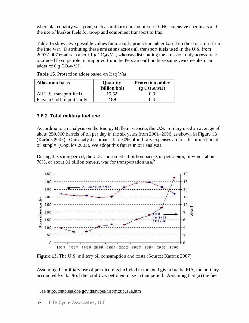
52| Life Cycle Associates, LLC
where data quality was poor, such as military consumption of GHG-intensive chemicals and
the use of bunker fuels for troop and equipment transport to Iraq.
Table 15 shows two possible values for a supply protection adder based on the emissions from
the Iraq war. Distributing these emissions across all transport fuels used in the U.S. from
2003-2007 results in about 1 g CO2e/MJ, whereas distributing the emission only across fuels
produced from petroleum imported from the Persian Gulf in those same years results in an
adder of 6 g CO2e/MJ.
Table 15. Protection adder based on Iraq War.
Allocation basis Quantity
(billion bbl)
Protection adder
(g CO2e/MJ)
All U.S. transport fuels 19.52 0.9
Persian Gulf imports only 2.89 6.0
3.8.2. Total military fuel use
According to an analysis on the Energy Bulletin website, the U.S. military used an average of
about 350,000 barrels of oil per day in the six years from 2001–2006, as shown in Figure 13
(Karbuz 2007). One analyst estimates that 50% of military expenses are for the protection of
oil supply (Copulos 2003). We adopt this figure in our analysis.
During this same period, the U.S. consumed 44 billion barrels of petroleum, of which about
70%, or about 31 billion barrels, was for transportation use.9
Figure 12. The U.S. military oil consumption and costs (Source: Karbuz 2007).
Assuming the military use of petroleum is included in the total given by the EIA, the military
accounted for 3.3% of the total U.S. petroleum use in that period. Assuming that (a) the fuel
9 See http://tonto.eia.doe.gov/dnav/pet/hist/mttupus2a.htm

53| Life Cycle Associates, LLC
as used has a life cycle global warming intensity (GWI) of about 95 g CO2e/MJ, (b) about
50% of all military operations are for the protection of oil supply, and (c) the protection of oil
supply is attributable to all transport fuels used in the U.S. from 2001-2006, we compute a
supply protection adder of about 1.6 g CO2e/MJ. Attributing these emissions only to transport
fuels from Persian Gulf oil imported during those years, the adder would be 7.1 CO2e/MJ as
shown in Table 16. The CO2 impact of oil field fires in Kuwait is discussed in the following
section.
Table 16. Protection adder based on Iraq War emissions.
Parameter Iraq War Kuwait Oil Fires
Daily fuel use 350,000 bbl/day 6,000,000 bbl/day
Duration 6 years 2.5 months
Assumed attribution 50% over
Allocation basis Crude Oil
Throughput
(billion bbl)
Protection
Adder
(g CO2e/MJ)
Protection Adder
(g CO2e/MJ)
All U.S. transport fuels 19.52 1.6 0.3
Persian Gulf imports only 2.89 7.1 1.4
3.8.3. Oil Field Fires
Another effect of Middle Eastern conflict occurred after the first gulf war in 1991. The
Kuwaiti oil fires were set by Iraqi military forces retreating from Kuwait. The fires burned
for over two months consuming 6 million barrels of crude oil per day (Figure 13). While such
an event can be considered a one time occurrence, the GHG emissions correspond to 1.4 g
CO2/MJ when assigned to Middle Eastern oil imports over a 20 year period.
Figure 13. USAF aircraft fly over Kuwaiti oil fires, set by the retreating Iraqi army during
Operation Desert Storm in 1991. Source www.af.mil/photos on www.wikipedia.com

54| Life Cycle Associates, LLC
3.8.4. Recommendations on Protection of Oil Supply
Addressing the GHG emissions associated with the protection of petroleum supplies presents
an ongoing challenge. Relating military activity to oil imports does not lend itself to a
straightforward attribution. Nonetheless, the connection between military expenditures,
military activity, and imported oil persists. Often government policy studies as well as life
cycle comparisons of fuel cite the military impacts of imported oil from an economic
perspective while calculations of GHG emissions exclude these effects. If the authors of such
studies can make the economic connection between Middle Eastern oil and petroleum, then
the GHG emission ought to also be examined as closely.
The calculations in this study show that the emissions are significant for the attribution and
time frame assumed in this study. Since the attribution of military activities to petroleum is
subjective, a clear path to improving the approach is not apparent.
3.9. Iraq Reconstruction
The Iraq war included significant destruction of infrastructure due to bombing, sabotage,
neglect, or other war related activities. Infrastructure includes buildings, roads, and bridges
whose construction requires energy intensive material inputs including concrete and steel. As
described below, cement production is a major component of these efforts.
3.9.1. Cement Production
Cement production is a significant contributor to global warming. The U.S. EPA estimates
that 3.4% of global CO2 emissions or 829 million metric tons are emitted during the cement
production process (Hanle 2004). This section provides an estimate of GHG emissions
associated with increased cement demand attributable to the Iraq reconstruction efforts. First,
the demand and supply situation for cement used in Iraq‘s reconstruction effort will be
detailed followed by a characterization of the GHG emission factor from the material‘s
production process. Combining cement demand with the emission factor results in the GHG
emissions from the reconstruction effort.
Iraq Cement Demand and Supply:
A recent article in Arabianbusiness.com asserts that Iraq‘s current annual cement production
from its seventeen production facilities totals between 4 to 5 millions tonnes. An additional 6
million tonnes is imported from Syria and Lebanon to increase current supply to 10 million
tonnes (Irish 2008). The supply estimates from this article are relatively consistent with
earlier statistical data from USAID, the 2006 U.S. Geological Survey and an article in the San
Francisco Chronicle (USAID-Iraq 2007), (Mobbs 2006), (Gilbert February 04, 2006).
Irish points out that Iraq cement demand before the war (before 2003) totaled approximately
10 million tonnes annually (Irish 2008). Current demand is estimated to be much higher in
large part due to the reconstruction efforts. The current annual demand is estimated to be 30
million tonnes (Atkin 2008). The cement demand attributable to reconstruction efforts is the
difference between current cement demand and the demand before the Iraq war: 20 million
tonnes annually. This is a first order approximation that does not take into account other

55| Life Cycle Associates, LLC
economic parameters such as price elasticity of demand or the influence of UN sanctions
imposed prior to the year 2003 on Iraq‘s cement demand.
CO2 Emissions from Cement Production:
Cement is produced by crushing limestone as well as other minerals such as iron oxides,
aluminum, silicon and pyro-processing the materials at high temperatures in special ovens,
called kilns (at 1500 ºC). Two basic processes exist: the ―wet‖ process mixes the crushed
material with water prior to kiln processing; the more modern ―dry‖ process feeds the material
directly to the kiln. Wet processing is more energy intensive and requires about 6
MMBtu/metric tonne; dry processing requires at least 6.9 MMBtu/metric tonne. On average,
kiln operation accounts for over 90% of the industry‘s energy needs (Hanle 2004). Regardless
of processing type, the resulting clinker material is cooled, ground, and additives such as
gypsum and lime are added to produce either Portland cement or masonry cement,
respectively.
Emissions factor for Iraq Cement Production:
The emissions from cement production fall into two categories: process and combustion
related emissions. The process emissions are created through the chemical decomposition of
calcium carbonate (e.g. from limestone) to calcium oxide and CO2, which results in direct
CO2 emissions through the kiln stack (Vanderborght 2001). Note that above it is stated that
calcium oxide is put into kilns, whereas here it is limestone. The World Business Council for
Sustainable Development (WBCSD) compiled a protocol for assessing CO2 emissions from
cement production. For process related emissions, the protocol proposes a default emission
factor of 0.525 tonnes CO2/tonne cement.
Combustion emissions are associated with generating the high energy requirements for the
kiln operation. World-wide kilns for clinker production are fueled by a variety of energy
sources. In the U.S.71% of kiln energy is provided by coal, 12% by petroleum coke, and the
rest by waste fuels (tires, garbage) and natural gas. Depending on the production method, the
carbon intensity factor of cement produced in the U.S. in 2001 ranged between 0.72 tonnes
CO2/tonne to 1.41 tonnes CO2/tonne (process and combustion emissions combined).
Worldwide, the average carbon intensity of cement production is on the low end of the U.S.
range at 0.83 tonnes CO2/tonne cement produced (OECD/IEA 2007). The lower emission
factor is likely due to a higher fraction of natural gas use in other countries (Taylor 2006).
Both the U.S. average and the World average cement emission factors, however, are likely not
representative of Iraq since all kilns there are fuel oil fired. Fuel oil has a higher emission
factor (166 lb/mmBtu) than natural gas (117 lb/mmBtu) but lower than coal (US-EPA Fifth
Edition).
Therefore, the combustion related emissions were reassessed using the fuel oil emission
factors taking into account that Iraq cement production utilizes about 50% wet and 50% dry
processes. The resulting combustion-related emission factor for Iraq cement is 0.577 tonnes
CO2/tonne. The process related emissions for Iraq cement are likely close to the WBCSD
default value of 0.525 tonnes CO2/tonne. Combining the combustion-related and the process
related emission factor for Iraq totals 1.102 tonnes CO2/tonne. This also brings to question
the requirement of imported cement and how that is transported.
56| Life Cycle Associates, LLC
3.9.2. GHG Emissions from Iraq Reconstruction Efforts
The GHG emissions from concrete used for the Iraq reconstruction effort is calculated by
multiplying the emission factor (1.102 tonnes CO2/tonne) by the annual cement demand
attributable to reconstruction (20 million tons). The resulting annual CO2 emissions from Iraq
cement production attributable to reconstruction are 22 million tonnes. Assuming a 5 year
reconstruction effort at this level, the total emissions from reconstruction total 110 million
tonnes. For reference purposes, the 2010 world CO2 emissions are projected to reach 31.1
billion tonnes (Energy Information Administration, 2008). Annual Iraq reconstruction efforts
will correspond to less than 0.1% of worldwide CO2 emissions.
3.9.3. Recommendations on Iraq Reconstruction
See Section. 3.8
4. Land use and other environmental impacts of petroleum
Petroleum production, transport, and refining require land and therefore have direct land use
impacts. Oil transportation also results in local environmental despoliation (e.g. the Niger
Delta), as well as oil spills. The GHG emissions associated with direct land use impacts (and
in some cases, their cleanup) are likely to be small relative to the total annual flow of oil.
Again, it would be appropriate to estimate these impacts to understand the order of magnitude,
and to maintain balance with regard to relative carbon LCA boundaries among different fuels
Land use impacts associated with the mining of tar sands, management of tailings, destruction
of natural forest, and emissions associated with reforestation are calculated in Section 6.2.
4.1. Deforestation following road construction
Road building in forested areas causes relatively small direct emissions, however the roads are
often a magnet for subsequent deforesting activities, providing access to previously
inaccessible land (NASA Earth Observatory 2008). The cited NASA report notes that:
Logging, both legal and illegal, often follows road expansion (and in some cases
is the reason for the road expansion). When loggers have harvested an area’s
valuable timber, they move on. The roads and the logged areas become a magnet
for settlers—farmers and ranchers who slash and burn the remaining forest for
cropland or cattle pasture, completing the deforestation chain that began with
road building.
Government-sanctioned (―official‖) roads begin a feedback process that promotes continued
expansion of road networks deeper into forested areas. In their review of road building and
land use change in the Amazon, Perz, Brilhante et al (2008) note:
Distinguishing between official and unofficial roads in the Amazon reveals an
important synergy: paving of official roads motivates unofficial road building. Paving
raises land values, which provides the incentive to exploit natural resources farther
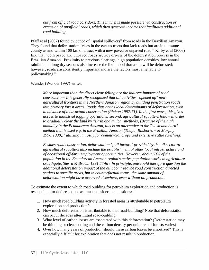
57| Life Cycle Associates, LLC
out from official road corridors. This in turn is made possible via construction or
extension of unofficial roads, which then generate income that facilitates additional
road building.
Pfaff et al (2007) found evidence of ―spatial spillovers‖ from roads in the Brazilian Amazon.
They found that deforestation ―rises in the census tracts that lack roads but are in the same
county as and within 100 km of a tract with a new paved or unpaved road.‖ Kirby et al (2006)
find that ―both paved and unpaved roads are key drivers of the deforestation process in the
Brazilian Amazon. Proximity to previous clearings, high population densities, low annual
rainfall, and long dry seasons also increase the likelihood that a site will be deforested;
however, roads are consistently important and are the factors most amenable to
policymaking.‖
Wunder (Wunder 1997) writes:
More important than the direct clear-felling are the indirect impacts of road
construction: It is generally recognized that oil activities "opened up" new
agricultural frontiers in the Northern Amazon region by building penetration roads
into primary forest areas. Roads thus act as local determinants of deforestation, even
in advance of their actual construction (Pichón 1997:71). In the first wave, this gives
access to industrial logging operations; second, agricultural squatters follow in order
to gradually clear the land by "slash and mulch" methods, [Because of the high
humidity in the Ecuadorean Amazon, this is an alternative to the "slash and burn"
method that is used e.g. in the Brazilian Amazon (Thapa, Bilsborrow & Murphy
1996:1330).] utilizing it mostly for commercial crops and extensive cattle ranching.
…
Besides road construction, deforestation "pull factors" provided by the oil sector to
agricultural squatters also include the establishment of other local infrastructure and
of occasional off-farm employment opportunities. However, about 60% of the
population in the Ecuadorean Amazon region's active population works in agriculture
(Southgate, Sierra & Brown 1991:1146). In principle, one could therefore question the
additional deforestation impact of the oil boom: Maybe road construction directed
settlers to specific areas, but in counterfactual terms, the same amount of
deforestation might have occurred elsewhere, even without oil production.
To estimate the extent to which road building for petroleum exploration and production is
responsible for deforestation, we must consider the questions:
1. How much road building activity in forested areas is attributable to petroleum
exploration and production?
2. How much deforestation is attributable to that road-building? Note that deforestation
can occur decades after initial road-building
3. What level of carbon losses are associated with this deforestation? (Deforestation may
be thinning or clear-cutting and the carbon density per unit area of forests varies)
4. Over how many years of production should these carbon losses be amortized? This is
especially difficult for exploration that does not result in production
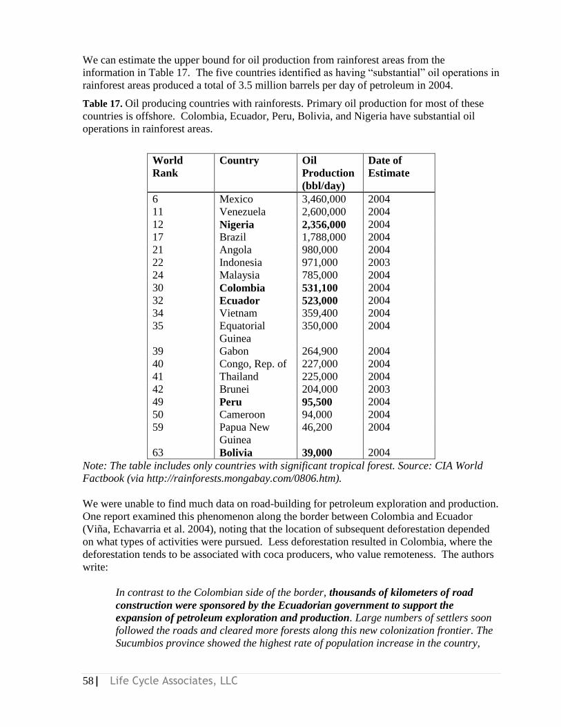
58| Life Cycle Associates, LLC
We can estimate the upper bound for oil production from rainforest areas from the
information in Table 17. The five countries identified as having ―substantial‖ oil operations in
rainforest areas produced a total of 3.5 million barrels per day of petroleum in 2004.
Table 17. Oil producing countries with rainforests. Primary oil production for most of these
countries is offshore. Colombia, Ecuador, Peru, Bolivia, and Nigeria have substantial oil
operations in rainforest areas.
World
Rank
Country Oil
Production
(bbl/day)
Date of
Estimate
6 Mexico 3,460,000 2004
11 Venezuela 2,600,000 2004
12 Nigeria 2,356,000 2004
17 Brazil 1,788,000 2004
21 Angola 980,000 2004
22 Indonesia 971,000 2003
24 Malaysia 785,000 2004
30 Colombia 531,100 2004
32 Ecuador 523,000 2004
34 Vietnam 359,400 2004
35 Equatorial
Guinea
350,000 2004
39 Gabon 264,900 2004
40 Congo, Rep. of 227,000 2004
41 Thailand 225,000 2004
42 Brunei 204,000 2003
49 Peru 95,500 2004
50 Cameroon 94,000 2004
59 Papua New
Guinea
46,200 2004
63 Bolivia 39,000 2004
Note: The table includes only countries with significant tropical forest. Source: CIA World
Factbook (via http://rainforests.mongabay.com/0806.htm).
We were unable to find much data on road-building for petroleum exploration and production.
One report examined this phenomenon along the border between Colombia and Ecuador
(Viña, Echavarria et al. 2004), noting that the location of subsequent deforestation depended
on what types of activities were pursued. Less deforestation resulted in Colombia, where the
deforestation tends to be associated with coca producers, who value remoteness. The authors
write:
In contrast to the Colombian side of the border, thousands of kilometers of road
construction were sponsored by the Ecuadorian government to support the
expansion of petroleum exploration and production. Large numbers of settlers soon
followed the roads and cleared more forests along this new colonization frontier. The
Sucumbios province showed the highest rate of population increase in the country,
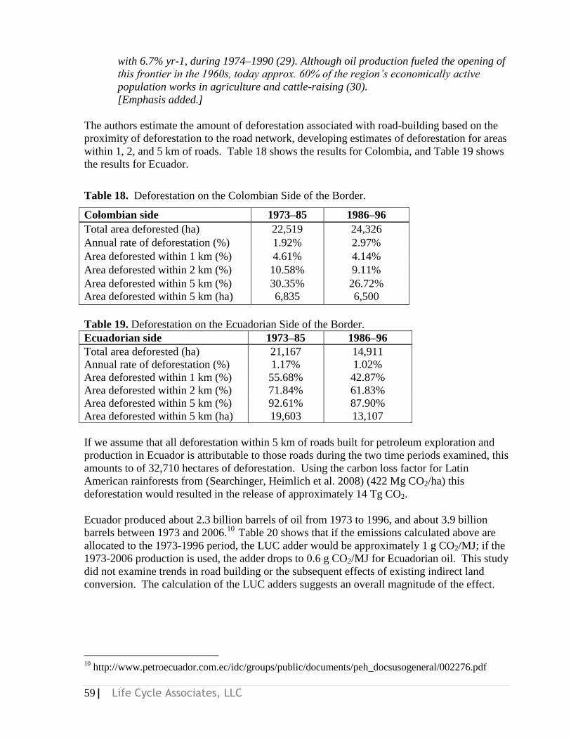
59| Life Cycle Associates, LLC
with 6.7% yr-1, during 1974–1990 (29). Although oil production fueled the opening of
this frontier in the 1960s, today approx. 60% of the region’s economically active
population works in agriculture and cattle-raising (30).
[Emphasis added.]
The authors estimate the amount of deforestation associated with road-building based on the
proximity of deforestation to the road network, developing estimates of deforestation for areas
within 1, 2, and 5 km of roads. Table 18 shows the results for Colombia, and Table 19 shows
the results for Ecuador.
Table 18. Deforestation on the Colombian Side of the Border.
Colombian side 1973–85 1986–96
Total area deforested (ha) 22,519 24,326
Annual rate of deforestation (%) 1.92% 2.97%
Area deforested within 1 km (%) 4.61% 4.14%
Area deforested within 2 km (%) 10.58% 9.11%
Area deforested within 5 km (%) 30.35% 26.72%
Area deforested within 5 km (ha) 6,835 6,500
Table 19. Deforestation on the Ecuadorian Side of the Border.
Ecuadorian side 1973–85 1986–96
Total area deforested (ha) 21,167 14,911
Annual rate of deforestation (%) 1.17% 1.02%
Area deforested within 1 km (%) 55.68% 42.87%
Area deforested within 2 km (%) 71.84% 61.83%
Area deforested within 5 km (%) 92.61% 87.90%
Area deforested within 5 km (ha) 19,603 13,107
If we assume that all deforestation within 5 km of roads built for petroleum exploration and
production in Ecuador is attributable to those roads during the two time periods examined, this
amounts to of 32,710 hectares of deforestation. Using the carbon loss factor for Latin
American rainforests from (Searchinger, Heimlich et al. 2008) (422 Mg CO2/ha) this
deforestation would resulted in the release of approximately 14 Tg CO2.
Ecuador produced about 2.3 billion barrels of oil from 1973 to 1996, and about 3.9 billion
barrels between 1973 and 2006.10
Table 20 shows that if the emissions calculated above are
allocated to the 1973-1996 period, the LUC adder would be approximately 1 g CO2/MJ; if the
1973-2006 production is used, the adder drops to 0.6 g CO2/MJ for Ecuadorian oil. This study
did not examine trends in road building or the subsequent effects of existing indirect land
conversion. The calculation of the LUC adders suggests an overall magnitude of the effect.
10
http://www.petroecuador.com.ec/idc/groups/public/documents/peh_docsusogeneral/002276.pdf
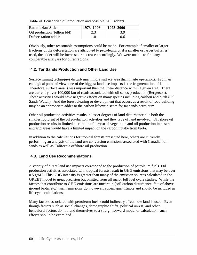
60| Life Cycle Associates, LLC
Table 20. Ecuadorian oil production and possible LUC adders.
Ecuadorian Side 1973–1996 1973–2006
Oil production (billion bbl) 2.3 3.9
Deforestation adder 1.0 0.6
Obviously, other reasonable assumptions could be made. For example if smaller or larger
fractions of the deforestation are attributed to petroleum, or if a smaller or larger buffer is
used, the adder will be increase or decrease accordingly. We were unable to find any
comparable analyses for other regions.
4.2. Tar Sands Production and Other Land Use
Surface mining techniques disturb much more surface area than in situ operations. From an
ecological point of view, one of the biggest land use impacts is the fragmentation of land.
Therefore, surface area is less important than the linear distance within a given area. There
are currently over 100,000 km of roads associated with oil sands production (Bergerson).
These activities would have negative effects on many species including caribou and birds (Oil
Sands Watch). And the forest clearing or development that occurs as a result of road building
may be an appropriate adder to the carbon lifecycle score for tar sands petroleum.
Other oil production activities results in lesser degrees of land disturbance due both the
smaller footprint of the oil production activities and they type of land involved. Off shore oil
production results in limited disruption of terrestrial vegetation and oil production in desert
and arid areas would have a limited impact on the carbon uptake from biota.
In addition to the calculations for tropical forests presented here, others are currently
performing an analysis of the land use conversion emissions associated with Canadian oil
sands as well as California offshore oil production.
4.3. Land Use Recommendations
A variety of direct land use impacts correspond to the production of petroleum fuels. Oil
production activities associated with tropical forests result in GHG emissions that may be over
0.5 g/MJ. This GHG intensity is greater than many of the emission sources calculated in the
GREET model to great precision but omitted from all major full fuel cycle studies. While the
factors that contribute to GHG emissions are uncertain (soil carbon disturbance, fate of above
ground biota, etc.); such emissions do, however, appear quantifiable and should be included in
life cycle calculations.
Many factors associated with petroleum fuels could indirectly affect how land is used. Even
though factors such as social changes, demographic shifts, political unrest, and other
behavioral factors do not lend themselves to a straightforward model or calculation, such
effects should be examined.
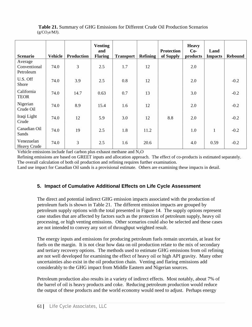
61| Life Cycle Associates, LLC
Table 21. Summary of GHG Emissions for Different Crude Oil Production Scenarios (g/CO2e/MJ).
Scenario Vehicle Production
Venting
and
Flaring Transport Refining
Protection
of Supply
Heavy
Co-
products
Land
Impacts Rebound
Average
Conventional
Petroleum
74.0 3 2.5 1.7 12 2.0
U.S. Off
Shore 74.0 3.9 2.5 0.8 12 2.0 -0.2
California
TEOR 74.0 14.7 0.63 0.7 13 3.0 -0.2
Nigerian
Crude Oil 74.0 8.9 15.4 1.6 12 2.0 -0.2
Iraqi Light
Crude 74.0 12 5.9 3.0 12 8.8 2.0 -0.2
Canadian Oil
Sands 74.0 19 2.5 1.8 11.2 1.0 1 -0.2
Venezuelan
Heavy Crude 74.0 3 2.5 1.6 20.6 4.0 0.59 -0.2
Vehicle emissions include fuel carbon plus exhaust methane and N2O
Refining emissions are based on GREET inputs and allocation approach. The effect of co-products is estimated separately.
The overall calculation of both oil production and refining requires further examination.
Land use impact for Canadian Oil sands is a provisional estimate. Others are examining these impacts in detail.
5. Impact of Cumulative Additional Effects on Life Cycle Assessment
The direct and potential indirect GHG emission impacts associated with the production of
petroleum fuels is shown in Table 21. The different emission impacts are grouped by
petroleum supply options with the total presented in Figure 14. The supply options represent
case studies that are affected by factors such as the protection of petroleum supply, heavy oil
processing, or high venting emissions. Other scenarios could also be selected and these cases
are not intended to convey any sort of throughput weighted result.
The energy inputs and emissions for producing petroleum fuels remain uncertain, at least for
fuels on the margin. It is not clear how data on oil production relate to the mix of secondary
and tertiary recovery options. The methods used to estimate GHG emissions from oil refining
are not well developed for examining the effect of heavy oil or high API gravity. Many other
uncertainties also exist in the oil production chain. Venting and flaring emissions add
considerably to the GHG impact from Middle Eastern and Nigerian sources.
Petroleum production also results in a variety of indirect effects. Most notably, about 7% of
the barrel of oil is heavy products and coke. Reducing petroleum production would reduce
the output of these products and the world economy would need to adjust. Perhaps energy

62| Life Cycle Associates, LLC
consumers would respond with the use of more coal but demand rationing, efficiency
improvements as well as a switch to natural gas and renewables are also options. Clearly,
more analysis is needed.
0
10
20
30
40
50
60
70
80
90
100
110
120
Avera
ge P
etro
leum
U.S
. Off
Shore
Califo
rnia T
EOR
Nigeria
n
Iraqi
Can
adian
Oil San
ds
Venez
uala H
eavy
Gaso
lin
e L
ife C
ycle
GW
I (g
/MJ)
Land Impacts
Heavy Coproducts
Protection of Supply
Refining
Transport
Venting and Flaring
Production
Fuel Combustion
Rebound
Figure 14. Summary of GHG Emissions for Different Crude Oil Production Scenarios.
Finally, petroleum production is associated with activities such as military operations in the
Middle East. The GHG impact of these operations is considerable when U.S. activities are
attributed to U.S. imports. While the 1% reduction in fuel use will not result in a 1%
reduction in Middle East military activity, the overall relationship must be taken into account
when assessing the impact of petroleum fuels.
The comparison of so many petroleum options that are a significant fraction of U.S.
consumption with emissions higher than the currently used average raises the question: Is the
average value correct?
The U.S. average value reflects conventional oil production and does not include Canadian oil
sands. The contribution of Canadian oil sands is a feature in the GREET model that is readily
calculated. Emissions associated with heavy oil production are embedded in the calculation
of the average. This subject requires more research. The emission estimate associated with

63| Life Cycle Associates, LLC
overseas venting and flaring appears optimistic with the assumption that they are two times
the U.S. value.
5.1. Uncertainties
The energy inputs and emissions associated with petroleum fuel production result in
considerable uncertainty, far more than attributed to the average. Uncertainties in the oil
production data, refinery allocation, and the treatment of co-products indicate at least a 5%
uncertainty for the average oil production. Figure 15 illustrates the total GHG emissions and
estimated uncertainty (on an additive basis) for each of the petroleum pathways examined
here. Significant ranges in emissions are related to the following:
Overseas vented natural gas
Oil sands processing technology
Treatment of co-product electricity from cogeneration
Method used to determine refinery emissions
Treatment of residual oil and coke co-products
0 20 40 60 80 100 120 140
Average Petroleum
U.S. Off Shore
California TEOR
Nigerian
Iraqi
Canadian Oil Sands
Venezuala Heavy
Gasoline Life Cycle GWI (g/MJ)
Figure 15. Range in GHG emissions for petroleum production scenarios.

64| Life Cycle Associates, LLC
6. References
Atkin, N. (2008). "2008 Provincial Reconstruction Team News." U.S. Embassy Baghdad
Public Affairs Section.
ARB (2008). ―Economic Analysis of the Draft Scoping Plan,‖ California Air Resources
Board Presentation, AB-32 Workshop, Sacramento, CA September 26, 2008.
ARB (2007). The Low Carbon Fuel Standard issued January 18, 2007. Retrieved from:
http://www.arb.ca.gov/fuels/lcfs/lcfs.htm
Aycaguer, A. C., M. Lev-On, et al. (2001). "Reducing carbon dioxide emissions with
enhanced oil recovery projects: A life cycle assessment approach." Energy & Fuels
15(2): 303-308.
Berk, P. (2006). Climate Change Modeling with EDRAM. UC Berkeley Presentation,
November 2006.
Bergerson, J. and D. W. Keith (2006). Life cycle assessment of oil sands technologies.
Alberta Energy Futures Project. Calgary, Alberta, Institute for Sustainable Energy,
Environment and Economy: 28.
BP (2008). Statistical Review of World Energy. British Petroleum, June 2008.
Brandt, A.R.; Farrell A. E., (2005). Scraping the Bottom of the Barrel: CO2 Emission
Consequences of a Transition to Low-Quality and Synthetic Petroleum Resources.
Proceedings of the 25th Annual North American Conference of the U.S. Association
for Energy Economics. September 2005.
Brinkman, N. et al. (2005). Well-to-Wheels Analysis of Advanced Fuel/Vehicle Systems— A
North American Study of Energy Use, Greenhouse Gas Emissions, and Criteria Pollutant
Emissions. General Motors, Argonne National Laboratory report.
Burnham, A., M. Wang, and Y. Wu (2006). Development and Applications of GREET 2.7 —
The Transportation Vehicle-Cycle Model, Energy Systems Division, Argonne
National Laboratory, ANL/ESD/06-5, November 2006.
Bemis, G., et al. (2003). Reducing California‘s Petroleum Dependence. California Energy
Commission/California Air Resources AB2076 Report P600-03-005F.
Clean Development Mechanism (CDM) (2007). A UNFCC Report CDM Reg. No. 0553:
Kwale CDM Monitoring Report. Retrieved from: www.cdm.unfcc.int
Copulos, M. R. (2003). America‘s Achilles Heel: The Hidden Costs of Imported Oil.
Washington, DC, The National Defense Council Foundation. Retrieved from:
http://ndcf.dyndns.org/ndcf/energy/NDCF_Hidden_Costs_of_Imported_Oil.pdf.
65| Life Cycle Associates, LLC
Delbianco, A. et al., (2008). Upgrading Unconventional Oil Resources
with the EST Process. Eni E&P Division, Eni R&M Division.
Delucchi, M. A. (2003). A Lifecycle Emissions Model (LEM): Lifecycle Emissions from
Transportation Fuels, Motor Vehicles, Transportation Modes, Electricity Use, Heating
and Cooking Fuels, and Materials. University of California, Davis, UCD-ITS-RR-03-
17 Main Report.
Delucchi, M. A. (2008). Incorporating Price Effects into Life Cycle Analysis. Presentation to
U.S. EPA, March 2008.
Delucchi, M. A. and J. J. Murphy (2008). "U.S. military expenditures to protect the use of
Persian Gulf oil for motor vehicles." Energy Policy 36(6): 2253-2264.
DfT (2008). Renewable Transport Fuel Obligation (RTFO). UK Department for
Transportation. Retrieved from: http://www.dft.gov.uk/pgr/roads/environment/rtfo/
DOE (2008). National Biofuels Action Plan. Biomass Research and Development Board.
October 2008.
Drilling, C. (2006). "Drilling rig information, rig 1." Retrieved July 13, 2006. Retrieved
from: http://www.cheyennedrilling.com/rig1.htm
Dusseault, M. (2002). ―Cold Heavy Oil Production with Sand in the Canadian Heavy Oil
Industry.‖ Prepared for Alberta Department of Energy, March 2002.
Edwards, R. (2007). ―Well-to-Wheels analysis of future automotive fuels and powertrains in
the European context,‖ JEC/CONCAWE/EUCAR, WELL-TO-TANK Report Version
2c, March 2007
Energy Information Administration (2008). "International Energy Outlook - 2008."
Retrieved from: http://www.eia.doe.gov/oiaf/ieo
Environmental Protection Agency (2008). "Climate Change: State and Local Governments:
Climate Action Team Report 2008‖. Retrieved from:
http://www.climatechange.ca.gov/climate_action_team/index.html
FAPRI (2008). Biofuels Impact of Selected Farm Bill Provisions and other BiofuelPolicy
Options. FAPRI-MU Report #06-08. Retrieved from: www.fapri.missouri.edu
Gilbert, B. (February 04, 2006). Iraq's new barrier to progress. Cement factories fall far short
of demand for reconstruction. San Francisco Chronicle.
Hanle, L. J. a. K. R. J., Joshua Smith (2004). "CO2 Emissions Profile of the U.S. Cement
Industry." U.S. Environmental Protection Agency.
66| Life Cycle Associates, LLC
ISO (2006). ISO 14044:2006 Environmental management -- Life cycle assessment --
Requirements and guidelines, (International organization for Standardization)
Irish, J. (2008). "Lafarge, Asiacell plan $550mn Iraq cement plant." Online Article Retrieved
from: http://www.arabianbusiness.com.
Kadam, K. L., V. Camobreco, et al. (1999). Environmental Life Cycle Implications of Fuel
Oxygenate Production from California Biomass. NREL/TP-580-25688, National
Renewable Energy Laboratory, Retrieved from:
http://www.nrel.gov/docs/fy99osti/25688.pdf.
Karbuz, S. (2007, 17 Feb). "US military oil pains." Retrieved 10 Jun 2008. Retrieved from:
http://www.energybulletin.net/26194.html.
Kenneth Small and Kurt Van Dender, (2005). The Effect of Improved Fuel Economy on
Vehicle Miles Traveled: Estimating the Rebound Effect Using U.S. State Data, 1966-
2001. UC Energy Institute Report.
Kirby, K. R., W. F. Laurance, A. K. Albernaz, G. Schroth, P. M. Fearnside, S. Bergen, E. M.
Venticinque and C. da Costa (2006). "The future of deforestation in the Brazilian
Amazon." Futures 38(4): 432-453.
Krauss, C. (2009). Where is Oil Going Next? The New York Times Source:
http://www.nytimes.com/2009/01/15/business/worldbusiness/15oil.html
Accessed January 15, 2009.
Larivé, J.F. (2008). "Fuels life cycle issues in generic studies and within a regulatory
framework - The European experience", CONCAWE presentation at California
Biomass Collaborative Workshop, June 2008.
Marano, J.J and Ciferno, J.P. (2001). Life-Cycle Greenhouse-Gas Emissions Inventory For
Fischer-Tropsch Fuels. Prepared for U.S. Department of Energy National Energy
Technology Laboratory.
Meyers, R. A. (1996). Handbook of Petroleum Refining Processes, Second Edition, McGraw
Hill.
Mobbs, P. (2006). 2006 Minerals Yearbook - Iraq, U.S. Geological Survey.
World Business Council for Sustainable Development.
NASA Earth Observatory. (2008). "Causes of Deforestation: Direct Causes." Retrieved
from: http://earthobservatory.nasa.gov/Library/Deforestation/
deforestation_update3.html. Accessed June 11, 2008.
NETL (2008). "Exploration & Production Technologies, Improved Recovery, Stripper Well
Technology," Retrieved from: www.netl.doe.gov/ Accessed December 2008.
67| Life Cycle Associates, LLC
OECD/IEA (2007). "Tracking Industrial Energy Efficiency and CO2 Emissions."
Oilsandswatch (2008). Pembrina Institute website on oil sands impacts. Retrieved from:
www.oilsandswatch.org.
OPEC (2007). World Oil Outlook 2007
OPEC (2008). World Oil Outlook 2008
OSTSEIS (2008). Oil Share and Tar Sands Programmatic EIS, Web site information center,
http://ostseis.anl.gov/.
OTS Heavy Oil Science Center (2008). Husky Oil Lloydminster Upgrader Launch Page,
Source: http://www.lloydminsterheavyoil.com/upgraderlaunch.htm
Patrick Hagen (2008). ―Slow steaming may not be slow enough‖ – Lloyd‘s List, 4,
September 2008
Perez, P. et al. (2001). ―Costs and Benefits of a Biomass-to-Ethanol Production Industry in
California‖, California Energy Commission P500-01-002A, March 2001.
Perz, S., S. Brilhante, F. Brown, M. Caldas, S. Ikeda, E. Mendoza, C. Overdevest, V. Reis, J.
F. Reyes, D. Rojas, M. Schmink, C. Souza and R. Walker (2008). "Review. Road
building, land use and climate change: prospects for environmental governance in the
Amazon." Philosophical Transactions of the Royal Society B: Biological Sciences
363(1498): 1889-1895.
Pfaff, A., J. Robalino, R. Walker, S. Aldrich, M. Caldas, E. Reis, S. Perz, C. Bohrer, E.
Arima, W. Laurance and K. Kirby (2007). "Roads and deforestation in the Brazilian
Amazon." Journal of Regional Science 47(1): 109-123.
RCF (2006). Effects of a Transition to a Hydrogen Economy on Employment in the United
States, Prepared for U.S. DOE by RCF Economic and Financial Consulting, Inc.
Reisch, N. and S. Kretzmann (2008). A Climate of War: The war in Iraq and global warming
Oilchange International, Retrieved from: http://priceofoil.org/wp-
content/uploads/2008.
Sandrea, I. and R. Sandrea (2007). "Exploration trends show continued promise in world's
offshore basins." Oil & Gas Journal 105(9): 34-+.
Sandrea, I. and R. Sandrea (2007). "Growth expected in global offshore crude oil supply." Oil
& Gas Journal 105(10): 34-+.
Schmidt, P. F. (1986). Fuel Oil Manual, Industrial Press, Inc.; 4 edition.

68| Life Cycle Associates, LLC
Searchinger, T., R. Heimlich, R. A. Houghton, F. Dong, A. Elobeid, J. Fabiosa, S. Tokgoz, D.
Hayes and T.-H. Yu (2008). "Use of U.S. Croplands for Biofuels Increases
Greenhouse Gases Through Emissions from Land Use Change." Science: 1151861.
Small, K. and K. Van Dender. (2007). Fuel Efficiency and Motor Vehicle Travel: The
Declining Rebound Effect. UC Irvine Economics Working Paper #05-06-03
Taylor, M., Cecilia Tam and Dolf Gielen (2006). "Energy Efficiency and CO2 Emissions from
the Global Cement Industry." International Energy Agency, Energy Technology Policy
Division Retrieved from:
http://www.iea.org/Textbase/work/2006/cement/taylor_background.pdf.
TDM Encyclopedia, (2008). Rebound Effects, Implications for Transport Planning.
Victoria Transport Policy Institute, http://www.vtpi.org/tdm/tdm64.htm, updated 22
July 2008.
UNFCC CDM KwaleNigerian Project No. 0782 (2006). Retrieved from:
http://cdm.unfccc.int/UserManagement/FileStorage/T2N9G73GCSUW91EJUE7BJRW9NGI
OLU. Report : November, 2006.
Unnasch, S., S. Huey, et al. (1996). Evaluation of Fuel Cycle Emissions on a Reactivity
Basis, Prepared for California Air Resources Board under Contract A166-134.
Unnasch, S. et al., (2001). Refinement of Selected Fuel-Cycle Emissions Analyses. ARB
Contract 98-338.
USDOC (1999). Economic Census - Crude Petroleum and Natural Gas Extraction: 1997. U.
C. B. U.S. Department of Commerce, U.S. Census Bureau.
USDOC (1999). Economic Census - Drilling Oil and Gas Wells: 1997. U. C. B. U.S.
Department of Commerce, U.S. Census Bureau.
USDOC (1999). Economic Census - Support Activities for Oil and Gas Operations: 1997. U.
C. B. U.S. Department of Commerce, U.S. Census Bureau.
USAID-Iraq (2007). "An Overview of the Iraq Cement Industry." Retrieved from:
http://www.izdihar-
iraq.com/resources/papers_pdfs/cement_industry_overview_rev3_acc_opt.pdf.
US-EPA (Fifth Edition). "Fuel Oil Combustion." Retrieved from:
http://www.epa.gov/ttn/chief/ap42/ch01/final/c01s03.pdf.
US Foreign Relations Committee. Hearing: "The Hidden Cost of Oil" March 30, 2006.
Martin R. Copulos, Dr. Hillard Huntington and Dr. Gary Yohe.
Vanderborght, B. a. U. B. (2001). The Cement CO2 Protocol: CO2 Emissions Monitoring and
Reporting Protocol for the Cement Industry

69| Life Cycle Associates, LLC
Viña, A., F. R. Echavarria and D. C. Rundquist (2004). "Satellite Change Detection Analysis
of Deforestation Rates and Patterns along the Colombia–Ecuador Border." AMBIO: A
Journal of the Human Environment 33(3): 118-125.
Wang, M. Q. (1999). GREET 1.5 - Transportation Fuel-Cycle Model - Volume 1:
Methodology, Development, Use, and Results. Argonne, Il, Argonne National
Laboratory: 239.
Wang, M., H. Lee, et al. (2004). "Allocation of energy use in petroleum refineries to
petroleum products - Implications for life-cycle energy use and emission inventory of
petroleum transportation fuels." International Journal of Life Cycle Assessment 9(1):
34-44.
Wang, M. (2008). Estimation of Energy Efficiencies of U.S. Petroleum Refineries. Argonne
National Laboratory.
Weiss, M. A. et al. (2008). ON THE ROAD IN 2035, Reducing Transportation‘s Petroleum
Consumption and GHG Emissions. Massachusetts Institute of Technology Laboratory
for Energy and the Environment Report No. LFEE 2008-05 RP
Wunder, S. (1997). From Dutch Disease to Deforestation - A Macroeconomic Link? A case
study from Equador. Copenhagen, Centre for Development Research, Danish Institute
for International Studies. Retrieved from:
http://dlc.dlib.indiana.edu/archive/00002873/01/wunder.pdf.
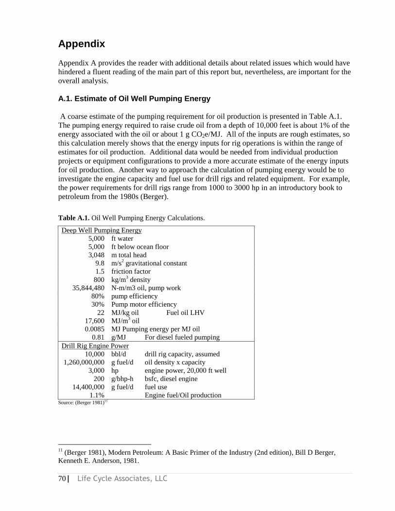
70| Life Cycle Associates, LLC
Appendix
Appendix A provides the reader with additional details about related issues which would have
hindered a fluent reading of the main part of this report but, nevertheless, are important for the
overall analysis.
A.1. Estimate of Oil Well Pumping Energy
A coarse estimate of the pumping requirement for oil production is presented in Table A.1.
The pumping energy required to raise crude oil from a depth of 10,000 feet is about 1% of the
energy associated with the oil or about 1 g CO2e/MJ. All of the inputs are rough estimates, so
this calculation merely shows that the energy inputs for rig operations is within the range of
estimates for oil production. Additional data would be needed from individual production
projects or equipment configurations to provide a more accurate estimate of the energy inputs
for oil production. Another way to approach the calculation of pumping energy would be to
investigate the engine capacity and fuel use for drill rigs and related equipment. For example,
the power requirements for drill rigs range from 1000 to 3000 hp in an introductory book to
petroleum from the 1980s (Berger).
Table A.1. Oil Well Pumping Energy Calculations.
Deep Well Pumping Energy 5,000 ft water 5,000 ft below ocean floor 3,048 m total head
9.8 m/s2 gravitational constant
1.5 friction factor 800 kg/m
3 density
35,844,480 N-m/m3 oil, pump work 80% pump efficiency 30% Pump motor efficiency
22 MJ/kg oil Fuel oil LHV 17,600 MJ/m
3 oil
0.0085 MJ Pumping energy per MJ oil 0.81 g/MJ For diesel fueled pumping
Drill Rig Engine Power 10,000 bbl/d drill rig capacity, assumed
1,260,000,000 g fuel/d oil density x capacity 3,000 hp engine power, 20,000 ft well
200 g/bhp-h bsfc, diesel engine 14,400,000 g fuel/d fuel use
1.1% Engine fuel/Oil production Source: (Berger 1981)11
11
(Berger 1981), Modern Petroleum: A Basic Primer of the Industry (2nd edition), Bill D Berger,
Kenneth E. Anderson, 1981.

71| Life Cycle Associates, LLC
These calculations could be illustrated with any range of assumptions so the key point of the
analysis is to demonstrate that pumping energy is within the 2 to 4% of energy required for
petroleum production with the possible exception for small stripper wells.
Oil producers could provide project specific data to help provide a better understanding of the
range in energy inputs for oil projects. The uncertain use of such data for regulatory purposes
would inhibit such an exercise. However, many oil producers already provide GHG emission
inventory data for corporate and government reporting requirements. Another approach could
be to examine engineering designs for oil production projects and relate all of the process
requirements and throughput into an emission intensity calculation.
A.2. Offshore oil production Energy Inputs and Emissions
Key points include:
The growing trend is to go deeper
Difficult to predict
Calculations are shown in Table A.2
Table A.2 Estimated Energy Inputs and Emissions from U.S. Offshore Oil Activities.
Off Shore Rig Activity
40000
hp
engines Exploration rig power
30% duty factor
24 h/day
160 g/bhph engine fuel consumption
3300 g/gal fuel density
800 rigs
Off Shore Oil Production
27 Mbbl/d Offshore oil capacity
1,134,000,000 gal/d Offshore oil production
Off Shore Energy Use and GHG Emissions
11,170,909 gal/d Engine Fuel Use
0.0099 J diesel energy/J product
95 g/MJ Diesel GHG factor
0.94 g/MJ Off Shore E&P
Heavy Oil Refining
Table 20 calculates the hydrogen requirements and assumed effect on gasoline production
emissions based on the hydrogen and carbon content of the feedstock oil. At a minimum,
sufficient hydrogen would be needed to make up for the hydrogen deficit in the heavy oil.
The oil compositions are based on data in the Fuel Oil Manual (Schmidt). These simple
calculations show that the hydrogen demand alone results in 6 to 9 g/MJ of GHG emissions
based on a hydrogen production-GHG factor of 95 g/MJ. Adding 25% for process heat and
utilities increases the effect of heavy oil processing to 8 to 12 g/MJ. These calculations also

72| Life Cycle Associates, LLC
indicate the magnitude of the emissions impact and more accurate values should be based on
modeling refinery and upgrader configurations.
Table 20. Calculation of GHG Emissions Associated with Hydrogen Deficit in Heavy Oil.
Crude Oil Type Conventional
Crude Oil Heavy
Crude
Oil
Light
Heavy
Oil
Units
API Gravity 27 10 16 H content 11.89% 10% 1.9% H/C, mole ratio 1.63 1.34 1.44 Mol Ratio Difference 0.29 0.19 0.02436 0.01596 kg H2/kg C 0.00245 0.00245 kg/scf H2 9.94 6.51 scf H2/kg C 3333 3333 g/gal 86.8% 88.6% 88.0% Oil Carbon Content 124028 123188 g C/bbl 1233 802 scf H2/bbl 80% 80% yield 1541 1003 scf H2/bbl gasoline 0.090 0.059 kg H2/gal gasoline 0.091 0.059 % gasoline energy 8.6 5.6 g GHG/MJ
Global offshore oil production in 2007 was approximately 27 mbbl/d, or some 33% of total
global oil production (Sandrea and Sandrea 2007). This percentage is only approximate and
will vary depending on 'what' is counted (only crude oil or all liquids).
Figure A.1 below shows offshore crude oil production over time. Shallow offshore
production has been maintained stable over the last ten years. Deep offshore activity
beginning from the late eighties has increased oil production to almost 5 mmbbl/d until 2007.
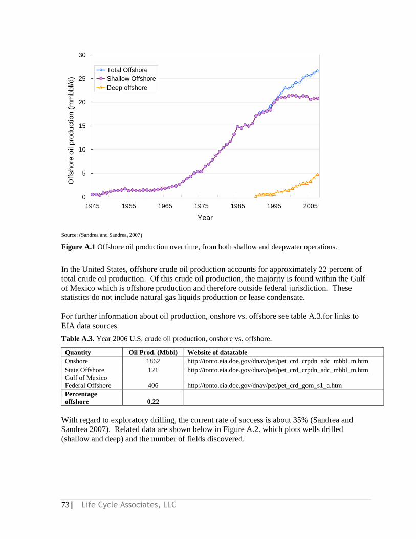
73| Life Cycle Associates, LLC
0
5
10
15
20
25
30
1945 1955 1965 1975 1985 1995 2005
Year
Off
shore
oil
pro
duction (
mm
bbl/d)
Total Offshore
Shallow Offshore
Deep offshore
Source: (Sandrea and Sandrea, 2007)
Figure A.1 Offshore oil production over time, from both shallow and deepwater operations.
In the United States, offshore crude oil production accounts for approximately 22 percent of
total crude oil production. Of this crude oil production, the majority is found within the Gulf
of Mexico which is offshore production and therefore outside federal jurisdiction. These
statistics do not include natural gas liquids production or lease condensate.
For further information about oil production, onshore vs. offshore see table A.3.for links to
EIA data sources.
Table A.3. Year 2006 U.S. crude oil production, onshore vs. offshore.
Quantity Oil Prod. (Mbbl) Website of datatable
Onshore 1862 http://tonto.eia.doe.gov/dnav/pet/pet_crd_crpdn_adc_mbbl_m.htm
State Offshore 121 http://tonto.eia.doe.gov/dnav/pet/pet_crd_crpdn_adc_mbbl_m.htm
Gulf of Mexico
Federal Offshore 406 http://tonto.eia.doe.gov/dnav/pet/pet_crd_gom_s1_a.htm
Percentage
offshore 0.22
With regard to exploratory drilling, the current rate of success is about 35% (Sandrea and
Sandrea 2007). Related data are shown below in Figure A.2. which plots wells drilled
(shallow and deep) and the number of fields discovered.

74| Life Cycle Associates, LLC
0
100
200
300
400
500
600
700
800
1935 1945 1955 1965 1975 1985 1995 2005
Year
Nu
mbe
r o
f w
ells
or
dis
cove
rie
s .
Shallow-water wells drilled
Deepwater wells drilled
Fields discovered
Figure A.2. Offshore exploratory drilling rates, shallow and deepwater.
The trends in these figures indicated growth in deep offshore production, which will be more
energy intensive and costly than comparable shallow water projects.
A.3.Trends in Petroleum Coke and Residual Oil Markets
Figure A.3. cites the worldwide trends of heavy oil consumption showing an overall decrease
in heavy oil consumption from about 11 mboe/day in 1997 to less than 10 mboe/day in 2007.
Source: BP 2008
Figure A.3. Worldwide trends in heavy oil consumption

75| Life Cycle Associates, LLC
Regional consumption of fuel oil
The most notable trend in demand by product is the continuing shift to middle distillates and
light products. Demand for residual fuel oil, including marine bunkers and refinery fuel, is
projected to remain stable, close to its current levels of around 10 mb/d. Residual fuel use in
the industry sector and for electricity generation will decline globally.
Oil for Power Generation
Despite the expected continued expansion in electricity production and consumption, the
prospects for oil demand growth in this sector are limited. In fact, there have been some
dramatic movements in this sector‘s oil usage over the past three decades.
For example, according to Figure A.4 in 1971 56% of the inputs to electricity generation in
the OECD Pacific was accounted for by oil, while by 2004 this had fallen to just 9%. This
movement was primarily in reaction to the oil price rises of the 1970s, which led to major
efforts to develop alternatives to oil in the electricity sector. Other OECD countries have also
reduced reliance on oil in this sector, with the region now accounting for an average of just
5% oil use in electricity generation. Developing countries are also generally using modest
volumes of oil. The most dramatic example in this sector is Southeast Asia, where the share
fell from 64% in 1971 to 9% in 2004. Many countries in Latin America, as well as OPEC
Member Countries, however, still rely upon oil for a large portion of electricity. Figure A.4.
shows that the oil share in electricity generation in 1971 compared to 2004 (OPEC).
Source: (OPEC 2007)
Figure A.4. Oil share in electricity generation: 1971 vs 2004 generated.
Coal continues to account for the largest share of electricity generated, although there are
considerable differences between world regions, which is largely attributed to resource
availability. For example, in 2004, coal accounted for as much as 50% of inputs to electricity
generation in North America, 71% in South Asia, and as much as 89% in China, all regions
with abundant coal reserves. Elsewhere, in regions such as Latin America and OPEC
countries, the average is well below 10%. Continued additions of coal-based generation
capacity, particularly in the U.S. and outside of the OECD, should mean that this fuel retains
its strong position in this sector. Indeed, in recent years, the U.S. has seen coal use grow faster
than natural gas.

76| Life Cycle Associates, LLC
However, the global share of natural gas has also risen steeply over the past two decades. For
example, in Western Europe in the early 1990s, gas accounted for just 6% of the inputs to
electricity generation, but this rose to 17% in 2004. Southeast Asia witnessed an even more
rapid rate of penetration, increasing from below 10% in 1990 to around 38% by 2004. Gas
has steadily consolidated its position as the fuel of choice in this sector in OPEC Member
Countries, accounting for over 50% of the inputs to electricity generation for the past ten
years. Throughout the world, gas-fired plants benefit from the efficiency of combined-cycle
technology, as well helping meet environmental concerns over the effect of emissions at both
local and global levels.
Some large developing countries are also considering developing nuclear power generation,
for example China and India. Even though renewables will rise over the next few decades,
they do from a low base, and thus their overall share is not likely to change dramatically.
Hydropower will witness a modest expansion, primarily in Asia and Central America.
With these developments in mind, it is not expected that oil demand will experience growth to
any significant degree in the electricity generation sector. As expected, no growth appears in
the OECD region. Similarly, within developing countries, continued switching leads to low
or no growth in China and Southeast Asia.
However, other developing country regions are expected to account for some growth,
amounting to a little over 1 mboe/d in total over the projection period. Table A.4. shows also
that North America well have a modest growth of oil consumption for electricity generation
until 2030 of about 0.2 mboe/d.
Table A.4. HFO, LFO and Diesel demand in electricity generation.
Region Demand Level (mboe/d) Growth
2006 2010 2020 2030 2006–2030
North America 1.1 1.1 1.2 1.3 0.2
Western Europe 0.8 0.7 0.7 0.6 –0.2
OECD Pacific 0.7 0.7 0.6 0.4 –0.3
OECD 2.6 2.6 2.4 2.4 –0.3
Latin America 0.3 0.3 0.3 0.3 0.0
Middle East & Africa 0.4 0.5 0.6 0.8 0.3
South Asia 0.3 0.3 0.4 0.5 0.2
Southeast Asia 0.2 0.2 0.2 0.2 0.0
China 0.3 0.3 0.2 0.2 –0.1
OPEC 1.3 1.4 1.5 1.5 0.2
Developing Countries 2.8 2.9 3.2 3.5 0.7
FSU 0.3 0.3 0.2 0.2 –0.2
Other Europe 0.1 0.1 0.1 0.0 0.0
Transition economies 0.4 0.4 0.3 0.2 –0.2
World 5.8 5.8 5.9 6.1 0.3 Source: OPEC 2008
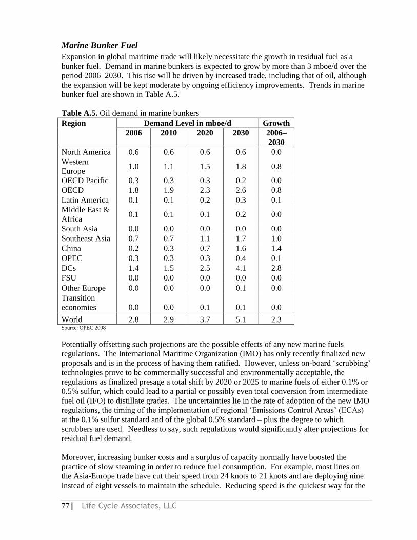
77| Life Cycle Associates, LLC
Marine Bunker Fuel
Expansion in global maritime trade will likely necessitate the growth in residual fuel as a
bunker fuel. Demand in marine bunkers is expected to grow by more than 3 mboe/d over the
period 2006–2030. This rise will be driven by increased trade, including that of oil, although
the expansion will be kept moderate by ongoing efficiency improvements. Trends in marine
bunker fuel are shown in Table A.5.
Table A.5. Oil demand in marine bunkers
Region Demand Level in mboe/d Growth
2006 2010 2020 2030 2006–
2030
North America 0.6 0.6 0.6 0.6 0.0
Western
Europe 1.0 1.1 1.5 1.8 0.8
OECD Pacific 0.3 0.3 0.3 0.2 0.0
OECD 1.8 1.9 2.3 2.6 0.8
Latin America 0.1 0.1 0.2 0.3 0.1
Middle East &
Africa 0.1 0.1 0.1 0.2 0.0
South Asia 0.0 0.0 0.0 0.0 0.0
Southeast Asia 0.7 0.7 1.1 1.7 1.0
China 0.2 0.3 0.7 1.6 1.4
OPEC 0.3 0.3 0.3 0.4 0.1
DCs 1.4 1.5 2.5 4.1 2.8
FSU 0.0 0.0 0.0 0.0 0.0
Other Europe 0.0 0.0 0.0 0.1 0.0
Transition
economies 0.0 0.0 0.1 0.1 0.0
World 2.8 2.9 3.7 5.1 2.3 Source: OPEC 2008
Potentially offsetting such projections are the possible effects of any new marine fuels
regulations. The International Maritime Organization (IMO) has only recently finalized new
proposals and is in the process of having them ratified. However, unless on-board ‗scrubbing‘
technologies prove to be commercially successful and environmentally acceptable, the
regulations as finalized presage a total shift by 2020 or 2025 to marine fuels of either 0.1% or
0.5% sulfur, which could lead to a partial or possibly even total conversion from intermediate
fuel oil (IFO) to distillate grades. The uncertainties lie in the rate of adoption of the new IMO
regulations, the timing of the implementation of regional ‗Emissions Control Areas‘ (ECAs)
at the 0.1% sulfur standard and of the global 0.5% standard – plus the degree to which
scrubbers are used. Needless to say, such regulations would significantly alter projections for
residual fuel demand.
Moreover, increasing bunker costs and a surplus of capacity normally have boosted the
practice of slow steaming in order to reduce fuel consumption. For example, most lines on
the Asia-Europe trade have cut their speed from 24 knots to 21 knots and are deploying nine
instead of eight vessels to maintain the schedule. Reducing speed is the quickest way for the

78| Life Cycle Associates, LLC
shipping industry to cut fuel consumption. Some owners have already begun to order new
vessels with smaller engines.
Petroleum Coke
There are several potential markets for pet coke. Petroleum coke is used in steel making and
also exported for power plant fuel. Note that the additional emissions associated with the
export of petroleum coke from U.S. refineries to Asia are not considered in life cycle
analyses.
The emissions for the base case gasoline production are also segmented by crude oil source
regions (CA, AK, and imports). The imported gasoline or crude oil can be considered the
marginal production resource. Emissions associated with residual oil and coke combustion
are about 10% of the total emissions when these co-products are represented in proportion to
gasoline fuel production. The appropriate allocation of these emissions would address how
these would change with a change in gasoline production.
0
20
40
60
80
100
120
140
160
180
200
-10% 10%
less
gasoline
Base Case more
gasoline
GH
G E
mis
sio
ns, W
TT
+ F
uel (T
g/y
)
Pet Coke Refining
Residual Oil Refining
Marketable Petroleum Coke
Residual Oil
Gasoline Refining
Gasoline Fuel
Figure A.5. Scenario for total GHG emissions associated with CA gasoline production.
Figure A.5. shows the energy inputs and GHG emissions associated with each of the fuel
categories. The combustion of co-products corresponds to 8 g CO2e/MJ of gasoline. All of
these emission reductions would not occur with a reduction in refinery output. The following
table A.6. shows the results of the calculations and the range in these indirect emissions.
CA
AK
Import
0
20
40
60
80
100
120
140
160
180
200
Source
Net Residual
+ Coke
Base Case Gasoline Life Cycle + Co-products

79| Life Cycle Associates, LLC
Table A.6. Energy Flows and Emissions Associated with Refinery Co-Products.
CA scenario less gasoline Base Case more
gasoline
-10% 10% Total Fuel Demand (bgal/y) 12.6 14 15.4
Energy (PJ/y) Gasoline 1499 1666 1833
Gasoline WTT (PJ/y) Gasoline Refining 457.3 508.1 558.9 Residual Oil 68.9 76.6 84.3 Marketable Petroleum Coke 65.2 72.5 79.7 Residual Oil Refining 0.43 0.48 0.52 Pet Coke Refining 0.48 0.53 0.59
Delta Gasoline (PJ/y) -167 0 167
GHG Emissions (Tg/y) Gasoline Fuel 108 120 132
Gasoline WTT Gasoline Refining 32.39 35.986 39.58
Co-products Residual Oil 4.45 4.942 5.44 Marketable Petroleum Coke 5.74 6.378 7.02 Residual Oil Refining 0.77 0.860 0.95 Pet Coke Refining 0.92 1.018 1.12
Total Co-product 11.9 13.2 14.5 Delta Co-product -1.320 0.000 1.320 Delta Co-product (g/MJ) 7.92 -- 7.92
A.4. Indirect Refinery Co-Product Emissions
The emissions associated with the use of residual oil are shown in Table A.7. These values do
not take into account market shifts in fuel usage. Residual oil comprises 4.6% of U.S.
refinery output. With a fixed refinery configuration, the amount of residual oil available on
the market would drop by this fraction. However, on the margin, imports from more remote
locations would be reduced if refinery output drops (or growth is limited). The average
distance for imported fuels to California is 7800 miles, which corresponds to about 1.1% of
the energy input to gasoline production. Thus, reducing gasoline output would reduce the
amount of residual oil that is produced, but less residual oil would be used for crude oil
transport.
Also shown are the emissions associated with electric power generation from fuel oil. 0.01
MJ of electric power could be produced from the net residual oil available from oil refining.
The emissions associated with the same amount of electric power from natural gas, coal, and
renewables is also shown as well as the net change in emissions. As indicated, switching

80| Life Cycle Associates, LLC
from residual oil to natural gas fired power would result in a GHG emission reduction of 1 g
CO2e/MJ of gasoline, while emissions would increase if coal were to displace residual oil
fired power. Of course, conservation or renewable power would reduce emissions further.
These emission estimates only bound the effect of residual oil production associated with
gasoline production as market forces could result in further fuel switching, conservation, and a
mix of these results.
Table A.7. Direct Emissions Associated with Residual Oil Usage and Electric Power Production.
WTT Attribution Energy Output and GHG Emission Savings
Residual Oil Production 0.046 J/J gasoline
Bunker Fuel for Crude Transport 0.011 J/J gasoline
Bunker Fuel
Less ship trade 3.3 g/MJ
Displaced Electric Power
Residual Oil Power Fuel 0.035 MJ Fuel Energy/MJ gasoline
Power Production Efficiency 0.32 MJe/MJ Residual Oil
Residual Oil Power 0.01 MJe/MJ Gasoline
Power Generation Emissions
Residual Oil Power 2.84 g CO2e/MJ Gasoline
NG Fired Power 1.69 g CO2e/MJ Gasoline
Coal Fired Power 3.70 g CO2e/MJ Gasoline
Renewable Power 0 g CO2e/MJ Gasoline
Net Difference
Residual Oil Power --
NG Fired Power 1.15 g CO2e/MJ Gasoline
Coal Fired Power -0.86 g CO2e/MJ Gasoline
Renewable Power 2.84 g CO2e/MJ Gasoline
Table A.6. shows a scoping calculation for the market mitigated effect of refinery co-products.
The GHG emissions associated with bunker fuel usage are multiplied by an assumed market
share and elasticity factor. The market share assumptions reflect the mix of fuel oil uses that
would be displaced and are provided for illustration purposes. The elasticity factor reflects
that fuel demand would respond to a reduction in supply. A 20% elasticity factor means that
fuel use is reduced by 20% and the remaining 80% of users find a substitute. In the case of
bunker fuel, crude oil could be a substitute. In the case of new sources of electric power
displacing crude oil, a 0% elasticity factor assumes that total power consumption remains
constant. A similar calculation is provided for petroleum coke. Here a 20% elasticity factor
refers to a reduction in total uses of petroleum coke. The remaining 80% would use
substitutes such as coal with comparable GHG emissions.
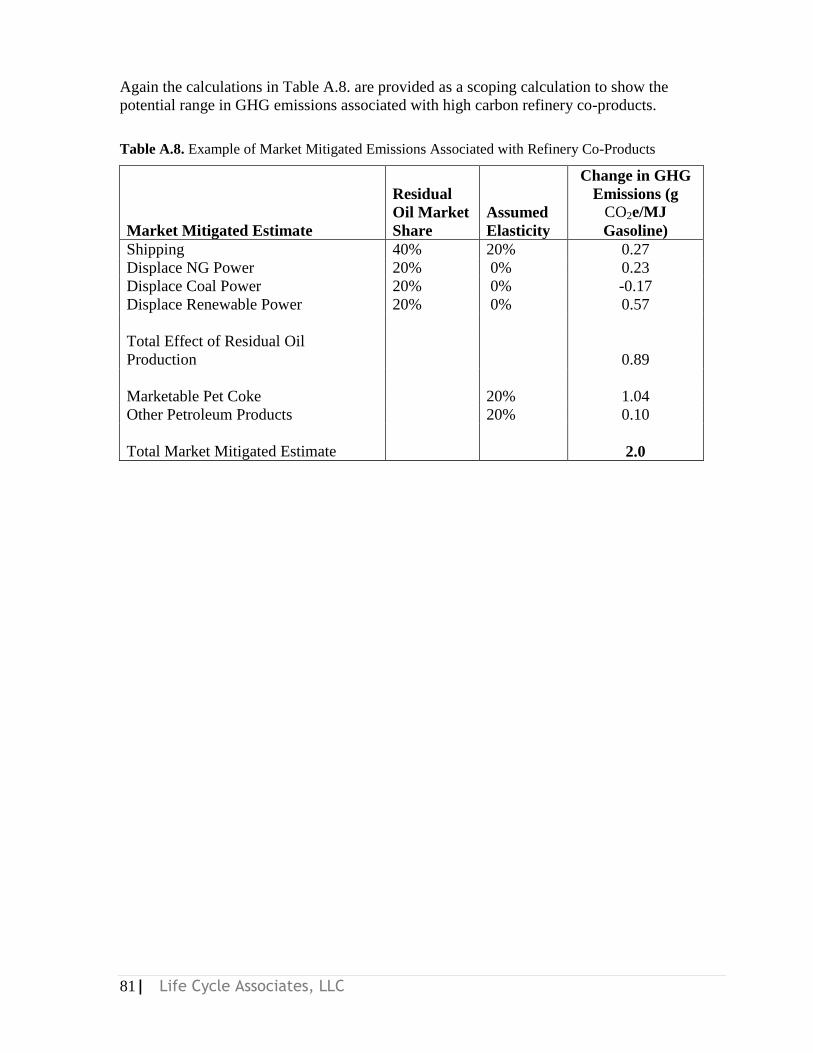
81| Life Cycle Associates, LLC
Again the calculations in Table A.8. are provided as a scoping calculation to show the
potential range in GHG emissions associated with high carbon refinery co-products.
Table A.8. Example of Market Mitigated Emissions Associated with Refinery Co-Products
Market Mitigated Estimate
Residual
Oil Market
Share
Assumed
Elasticity
Change in GHG
Emissions (g
CO2e/MJ
Gasoline)
Shipping 40% 20% 0.27
Displace NG Power 20% 0% 0.23
Displace Coal Power 20% 0% -0.17
Displace Renewable Power 20% 0% 0.57
Total Effect of Residual Oil
Production 0.89
Marketable Pet Coke 20% 1.04
Other Petroleum Products 20% 0.10
Total Market Mitigated Estimate 2.0