Assessment in Calculus in the Presence of Graphics Calculators · Assessment in Calculus in the Presence of Graphics Calculators ... appropriate to the task at hand, ... can be represented

Mathematics Education Research Journal 2002, Vol. 14, No. 1, 16-36

Assessment in Calculus in the Presence of GraphicsCalculators

Patricia A. Forster and Ute MuellerEdith Cowan University

In this paper we explore the extent and nature of students’ calculator usage asdetermined from examination scripts in the Western Australian Calculus TertiaryEntrance Examination. Errors made and understanding called upon are discussedfor seven questions. The inquiry highlights that skills associated with graphicalinterpretation need to be the subject of instruction, and that an awareness of thediffering cognitive demands of graphical interpretation is needed when settingassessment items.

Graphics calculators have been assumed equipment in Western AustralianTertiary Entrance Examinations (TEE) for mathematics, chemistry, and physicssince 1998. This paper reports our findings on the extent and nature of students’ useof graphics calculators in the 1999 Calculus TEE. We discuss results for sevenquestions from the 20-question paper. A major part of the inquiry is to consider thetypes of mathematical understanding called upon in calculator-assisted solutions.Implications of the examination outcomes for teaching and assessment arediscussed.

The significance of the paper is that it reports examination outcomes for alarge cohort in an upper-secondary context, where graphics calculators wererequired. Others (e.g., Anderson, Bloom, Mueller, & Pedler, 1997; Brown &Neilson, 2001; Jones & McCrae, 1996; Kemp, Kissane, & Bradley, 1997) discussdirections for assessment with the technology and analyse assessment questions,but few empirical studies focus on student performance in formal examinations.Exceptions are the studies in tertiary settings by Berger (1998) and Boers and Jones(1994). Other papers from the study of which this paper is part include a criticalscrutiny of the Calculus TEE questions for 1996-1999 (Mueller & Forster, 2000),investigation of gender-related effects 1995-2000 (Forster & Mueller, in press) andqualitative and quantitative analyses of students’ performance in the 1998Calculus TEE (Forster & Mueller, 2001).

Interpretative Framework

Mathematical UnderstandingVarious types of mathematical understanding are distinguished in the

literature. In our analysis we rely on the categories operational understandingand structural understanding (Sfard, 1991). Operational understanding entailsconceiving a mathematical notion to be the result of a sequence of “processes,algorithms and actions” (p. 4). Structural understanding is indicated if a notion isreferred to as an object or “static structure” (p. 4). Typically, operationalunderstanding precedes structural understanding. However, development mightbe in the reverse order, that is structural to operational, especially for geometry

Assessment in Calculus in the Presence of Graphics Calculators 17

(Forster & Taylor, 2000; Sfard, 1991).Others classify understanding in similar ways. For example, Hiebert and

Carpenter (1992) use the terms procedural and conceptual. Nesher (1986)differentiates between algorithmic performance and mathematical understand-ing. Gray and Tall (1994) refer to understanding processes and understandingconcepts. In addition, Gray and Tall (1994) distinguish processes from procedures.For them, a procedure “is a specific algorithm for implementing a process” (p.117). Thus, processes such as addition have meaning even when they are notenacted. We draw on this distinction in the analysis.

To elaborate the above definitions, we consider the example of limits.Evidence of operational understanding of the limit

limx →a

f(x ) could be the

evaluation of a given function f for values close to a specified value of a and oneither side of a, using the table of values on a graphics calculator. The table ofvalues procedure results in a value for the limit, provided that limit exists.Structural understanding is said to be present when the student recognises limitsor limiting values as having meaning separate from the processes that generatethem: general properties of the category limit can be investigated, as can “thevarious relations between its representatives” (Sfard, 1991, p. 20). A next stage ofdevelopment could involve a new category, the derivative, emerging from thelimit concept. The derivative of a function at a point could be understoodoperationally as the limit of the slopes of secant lines, and a graphics calculatorcould be used to explore numerically and visually this concept. Over time, thederivative (or derivative function) might be understood as a structure in its ownright and its properties discovered.

Characteristically, successful mathematics students can interpretmathematical notation in terms of operations and structures, whichever isappropriate to the task at hand, and they recognise that a mathematical objectcan be represented in multiple ways (Gray & Tall, 1994). However, many studentsdo not proceed beyond operational understanding. They progress through thecurriculum with pseudostructural thinking (Sfard & Linchevski, 1994). So, theylearn and apply algorithms and, therefore, operate on mathematical objects, butdo not understand the nature of those objects. As a result, their ability to applytheir knowledge in unusual or unfamiliar contexts is limited.

There is empirical evidence that graphical approaches on a graphicscalculator can facilitate both types of understanding of the function concept (e.g.,Hollar & Norwood, 1999), and the use of numerical calculation capabilities canadvance structural understanding. For instance, equations can be entered in thesolve facility on some calculators, values for all variables except one entered, andthe calculator will produce a value for the non-specified variable. Theexpressions that are entered can be conceived in terms of the processes shown (forexample, addition) or, because the solution procedures are hidden, the input-output tasks can foster understanding about the relationships between thevariables, that is, structural understanding (Forster & Taylor, 2000; Tall &Thomas, 1991).

18 Forster & Mueller

Assessment, Understanding, and Graphics CalculatorsIssues of assessment in the presence of graphics calculators include

accessibility of calculators. In Western Australia graphics calculators have beenrequired for mathematics tertiary entrance examinations since 1998. Non-symbolic graphics calculators and the Hewlett Packard HP38G and HP39G withlimited symbolic capabilities are approved for examination purposes. In 1998 and1999, students were asked to write the brand of their calculator on theirexamination scripts and access was universal for this cohort (Alguire & Forster,1999).

Other assessment issues are the types of understanding that should be tested,and the scope for use of the calculators. Senk, Beckmann, and Thompson (1997)conducted a major inquiry into test items used in 19 high-school mathematics(precalculus) classrooms where graphics calculators and other computertechnologies were used for learning. They developed a classification scheme forthe characteristics of test items and found high emphasis on the ability to applyalgorithms and low calls on technology usage in the test items that theycollected. We modified the scheme to suit calculus (Mueller & Forster, 2000) andused it to code the questions in the Calculus TEE for 1996-1999. Our analysisshowed that the percentages of part questions that tested algorithmiccompetence were 70% in 1996, 80% in 1997, 67% in 1998 and 65% in 1999. The highpercentages reflected the findings of Senk et al. (1997), but changes were evidentin 1998-1999 upon the introduction of the calculators. In the curriculum component,Applications of Calculus, there was a move towards interpretative questionswhere graphics calculator usage was an option. Diagrams, including calculator-generated graphs, played a greater role in Functions and Limits than previously,and fewer marks were allocated to algebraic procedures than in 1996-1997.Complex Numbers was the curriculum component most affected by the introductionof calculators. Questions needed a greater number of steps to reach an answer,called on more reasoning, and fewer questions relied on the application of analgorithm.

Our inquiry (Mueller & Forster, 2000) showed also that there was lessopportunity for graphics calculator usage in the 1998-1999 Calculus papers thanin 1996-1997, had the technology been allowed. This difference is explained bythe presence in 1996-1997 of procedural questions that are trivialised by thetechnology.

Examination Performance in CalculusBoers and Jones (1994) found in the final examination of a first university

calculus course that “the calculator was underutilized by most students” (p. 491).In particular, students showed a preference for analytic methods for limits, eventhough graphical and numeric approaches on the calculator had beenemphasised in lectures. For a limit that was difficult to determine analytically,those students who chose a calculator method made errors that indicated a naïveinterpretation of the relevant calculator graph, or data/formula entry mistakes.When asked to graph a rational function, many students did not include criticalfeatures on their hand-drawn graphs, which Boers and Jones (1994) explain as


failure to integrate algebraic information in the question with the graphicaldisplay on the calculator. We observed similar under-utilisation of thetechnology for limits and problems with graphing in the 1998 Calculus TEE(Forster & Mueller, 2001). Graphing rational functions with their asymptotes andpoint discontinuities seems a source of major difficulty. Ward (1997) also recordedthat students make errors in these areas.

Berger (1998), in the setting of first year university calculus, investigated twopossible effects of graphics calculator usage: effects on ability when workingwith technology (due to human working memory being freed from calculation) andeffects on conceptual understanding that result from using it. The first effect wasidentified, but students’ examination and test answers (completed without thetechnology) indicated that calculator use over one year did not result in studentsapproaching their mathematics in significantly different ways or in gainingdeeper understanding of calculus concepts. Berger attributed these outcomes to thetechnology being used during the calculus course only as an add-on tool to supportand verify traditional analytic methods.

Thus, sites of error in calculator-based solutions in calculus and constrainingeffects of instruction with the technology have been identified. On the otherhand, passing calculation to the technology can be beneficial, and inquiries innon-calculus settings have shown that if calculator approaches are a focus ofinstruction then insightful and different understandings can result (e.g., Hollar &Norwood, 1999; Schwarz & Hershkowitz, 1999).

Overview of the ResearchThree research questions guided our inquiry into the 1999 Calculus TEE.

• How might students have utilised their graphics calculators inanswering examination questions and what errors did they make thatwere associated with calculator usage?

• What types of understanding are called upon in graphics-calculatorassisted solutions to the examination questions?

• What are the distributions and mean scores for students using graphicscalculator approaches and students using traditional methods on theexamination questions where graphics calculator use was viable?

Accordingly, prior to the examination, we selected for inquiry sevenexamination questions that were either graphics calculator active, where use ofthe tool is necessary or greatly simplifies the solution, or neutral, where use ofthe tool is a viable option (Senk et al., 1997). We collected four types of data:interviews with students; marks for all candidates; details of students’ answersrecorded by markers; and our own observations of students’ written answers, madein our roles as examiners and markers.

Ten students were interviewed in the three days following the examination.The purpose of the interviews was to ascertain how the students had answeredthe examination questions, specifically, how they had used their graphicscalculators. Three students from each of two schools and four from another wereinterviewed. The students were selected by their teachers on the basis of being


communicative. Their school assessment grades ranged from A to C (D is thelowest grade). The examination paper was the focus of discussion in theinterviews. The interview data were used in answering the first and secondresearch questions.

The Curriculum Council supplied us with the marks for each candidate foreach examination question, and with summary statistics, including thecoefficients of correlation between the total and each question. In addition, markswere collected and made available to us for the two part questions that weanticipated would attract the widest calculator usage (Questions 6d and 13c).This data contributed to answering the third research question.

The Curriculum Council also supported us in obtaining from markers the partmarks for seven questions, and markers’ opinions on the nature of students’methods (traditional or calculator based) that they recorded by ticking columnson a proforma. Graphics calculator usage was optional for the seven questions.The data was collected for 20% of the scripts from the first marking round only(scripts are marked twice) and participation in the collection was voluntary.Nine out of 24 markers volunteered to be involved. All markers were experiencedteachers and the result was data for 195 scripts, from a total of 1937 scripts. Thisdata was used in answering the third research question.

The fourth source of data was our own observations, which we recorded whilemarking 240 scripts. We made notes and collected data on (a) the seven questionsselected for the research so that we had information on these for 435 candidatesin all, and (b) on an additional question, that emerged as interesting during themarking. Graphics calculator usage turned out to be difficult to discern for two ofthe seven questions and we did not pursue analysis of the outcomes on them. Insummary, in the results section we discuss one question for which we had marksfor the whole population (Question 6d, N = 1937) and five questions for which wehad qualitative data and part marks (Questions 7, 12, 13, 14 and 20; n = 435), andQuestion 8 (n = 240).

Our method was to conduct a qualitative analysis of students’ interview dataand our own notes. Statistical analysis of the sample data followed, to determinehow many students adopted traditional methods and how many seemed to usecalculator approaches. Limitations were that the scripts from which data werecollected were not randomly selected and determination of the methods studentsused relied on subjective judgement. However, we ascertained that our sample (n =435) is representative for the population via a chi-squared goodness of fit test.This test showed that the total raw examination scores of the sample had thesame distribution as the population, χ2 (13, N = 435) = 8.56. We present a summaryof students’ marks and a description of the nature of their responses for eachquestion, and an analysis of types of understanding called upon, for graphicalsolutions in particular. Mean scores for the population are based on numbers ofstudents who attempted the questions. For the sample data, means are calculatedfor students whose methods were recorded. Some students’ methods were notrecorded as being calculator-based or traditional because they were difficult todiscern, and some students did not attempt all questions, resulting in discrepanciesbetween the sample size and the number of students accounted for in the summarytables.


Results and Discussion

Graphics Calculator Evaluation of a Definite Integral

Question 6(d): Find the integral

1 − 2 sin2 x dx0

π /6

∫ .

Solution: 0.47 (2 d.p.) [3 marks]

The integral in Question 6d cannot be obtained analytically so studentsneeded to use their graphics calculators. Table 1 is a summary of students’ scores.Results are included for Questions 6a-c, which required evaluation of indefiniteintegrals and where graphics calculator use was not possible or not practical,depending on the model of calculator. The percentage mean scores are thepercentage of the total marks available for the questions (e.g., 52% = 1.56 out of3).

Table 1Evaluation of Indefinite Integrals (Question 6a-c) and a Definite Integral(Question 6d)

6a-c 6d

No. of students attempting the questions (N=1937) 1892 1774Mean score 6.65 (60%) 1.56 (52%)No. who scored zero 29 814

Altogether, nearly 50% of candidates did not attempt Question 6(d), or scoredzero for it. Explanations that emerged in the interviews were that students:

• did not recognise the need to use their calculators;• did not know how to evaluate the integral on their calculator, which

included not knowing the syntax; and/or• did not have time to return to the question after missing it out or

abandoning it.

Some scripts showed answers that were consistent with calculators set indegree mode rather than the required radian mode. In summary, the resultshighlight the importance of appreciating and understanding calculatorfunctionality, and show that half the candidature did not display the necessaryknowledge.

Identification of Maximum Stationary Point and Evaluation of Area

Question 7: Suppose that f( x ) =

3cosx

2 + sin x, − π ≤ x ≤ π .

(a) Determine exactly the two zeroes r1 and r2 of f.(b) Calculate the exact co-ordinates of the maximum stationary point.(c) Determine the area of the region above the x-axis bounded by the x axis and thegraph of f.


Solution:(a) x = ± π /2 [2 marks]

(b) Max stationary point = ( −π/ 6, 3 ) [5 marks]

(c)

3cos x/(2 + sin x) dx−π /2

π/ 2

∫ = 3 ⋅30 (2 d.p.) [3 marks]

For Questions 7b and c markers were asked to indicate traditional method(working shown) or calculator approach (the answer only), together with partmarks, and whether exact values were given in 7b. The results are summarised inTable 2. Data were not gathered for 7a as the zeroes of the cosine function in theinterval [–π, π] would be subject to recall by many students, therefore, calculatorusage would be impossible to discern on the basis of no working.

Table 2Determining a Maximum Turning Point (Question 7b) and Area (Question 7c)

7b 7c

Traditional Graphicscalculator


Number of students (n = 435)

311 99 73 300

Mean score 4.1(81%) 3.8(76%) 1.9(63%) 2.5(84%)Number who scored zero 8 5 14 17% who gave exact values 89% 74% - -

Note. The χ2–value for goodness of fit between sample and population data is χ2(8, N = 435) = 6.45.

For 7b, about three-quarters of scripts in the sample showed an analytic(traditional) method. Interviewed students said a reason for the choice was therequirement of exact values. Some said that they combined the analytic methodwith graphics calculator use for determination of the co-ordinates of thestationary point, or used the calculator to check the coordinates. Calculator useinvolved:

• entering into the calculator the function, together with the derivativecommand, setting the expression equal to zero, and solving the equation ina numerical solve facility; and

• graphing the function (which could be done from the start) then using thebuilt-in capabilities of the calculator to obtain the co-ordinates of theturning point (see Figure 1).

Derivatives that were not simplified in written answers and sketches of thefunction indicated also a combination of methods.

An error with answers obtained analytically was to locate the maximumpoint at x = π/6 instead of at x = –π/6. However, the percentage of students whofailed to convert decimal approximations to exact values was greater for thegroup who relied solely on a calculator solution, which explains the lower meanmark. The interviewed students who did the conversion said they recognised the


decimal was –π/6 or converted it using the routine of dividing by π to obtain the1/6; and they recognised the second coordinate was √3.

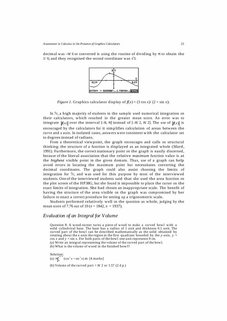
Figure 1. Graphics calculator display of f(x) = (3 cos x)/(2 + sin x).

In 7c, a high majority of students in the sample used numerical integration ontheir calculators, which resulted in the greater mean score. An error was tointegrate

f(x) over the interval [-π, π] instead of [–π/2, π/2]. The use of f(x) is

encouraged by the calculators for it simplifies calculation of areas between thecurve and x axis. In isolated cases, answers were consistent with the calculator setto degrees instead of radians.

From a theoretical viewpoint, the graph encourages and calls on structuralthinking: the structure of a function is displayed as an integrated whole (Sfard,1991). Furthermore, the correct stationary point on the graph is easily discerned,because of the literal association that the relative maximum function value is atthe highest visible point in the given domain. Thus, use of a graph can helpavoid errors in locating the maximum point but necessitates converting thedecimal coordinates. The graph could also assist choosing the limits ofintegration for 7c, and was used for this purpose by most of the interviewedstudents. One of the interviewed students said that she used the area function onthe plot screen of the HP38G, but she found it impossible to place the cursor on theexact limits of integration. She had chosen an inappropriate scale. The benefit ofhaving the structure of the area visible on the graph was compromised by herfailure to enact a correct procedure for setting up a trigonometric scale.

Students performed relatively well on the question as whole, judging by themean score of 7.76 out of 10 (n = 1842, n = 1937).

Evaluation of an Integral for Volume

Question 8: A wood-turner turns a piece of wood to make a curved bowl with asolid cylindrical base. The base has a radius of 1 unit and thickness 0.1 unit. Thecurved part of the bowl can be described mathematically as the solid obtained byrotating about the x-axis the region in the first quadrant bounded by the y-axis, y =cos x and y = sin x. For both parts of the bowl one unit represents 9 cm.(a) Write an integral representing the volume of the curved part of the bowl.(b) What is the volume of wood in the finished bowl?

Solution:(a)

π (cos2 x − sin 2 x) dx

0

π /4

∫ [4 marks]

(b) Volume of the curved part = π/2 or 1.57 (2 d.p.)


Total volume = (π/2 + πx1 2x0.1) x 93 cm3 = 1374 cm3 [4 marks]

For Question 8, we recorded the nature of students’ answers for the 240 scriptsthat we marked and the results are summarised in Table 3. Incorrect answers forthe integral with a calculator evaluation (inferred from no working shown)caught our attention and led to the data collection.

Table 3Evaluation of an Integral for Volume (Question 8)

Traditional Graphics calculator

Part (a)Correct

Part (a)Incorrect

Part (a)Correct

Part (a)Incorrect

Number of students(n = 240)

23 31 43 65

Number with correctevaluation

20 14 31 38

The proportion of the graphics calculator group with Part (a) correct whoevaluated the integral correctly was 72%. Further, of the students in the samplewho chose to use their graphics calculator to evaluate the integral that they hadobtained, only 64% succeeded in obtaining a value consistent with their integral.Entry and/or syntax errors are salient.

The mean mark for the question as a whole for the cohort was low (3.78 out of8, n = 1728).

Solution of a Non-linear Equation

Question 12: The difference between high and low water tide levels in one of theports along the northwest coast of Western Australia is 6 metres. At the entrance ofthe port from the ocean, the level x of water is given by

d 2xdt 2 = − 1

4x where t is

measured in hours from the time of the low tide.(a) Calculate the amplitude and the period of the motion of the tides.(b) Write x as a function of t.(c) A ship can enter or leave the port as long as there is at least one metre of waterabove the low tide mark. If the low tide takes place at 10:15 am, what is the latesttime a ship can leave the port on that day?

Solution:(a) amplitude = 3m, period = 4π hours [3 marks](b) x = –3cos(t/2) is one possible answer. [3 marks](c) –3cos(t/2) = –2, t = 10·8842, Time = 10:15 am + 653·05mins = 9:08 pm [5 marks]

Sample data were generated for 12c and are summarised in Table 4.Calculator use was inferred from no working or the provision of a graph only.Except for checking in 12b that would be impossible to infer, the other partquestions were calculator inactive, so were not considered in the data collection.


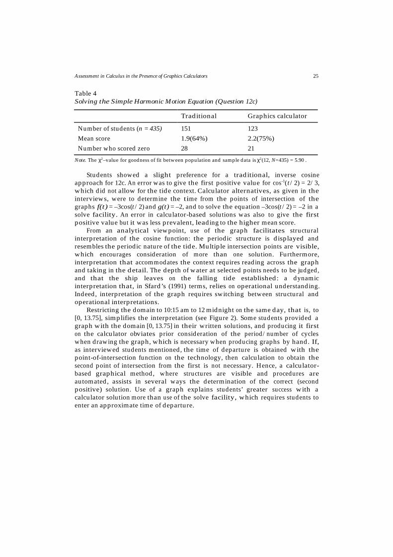
Table 4Solving the Simple Harmonic Motion Equation (Question 12c)

Traditional Graphics calculator

Number of students (n = 435) 151 123Mean score 1.9(64%) 2.2(75%)Number who scored zero 28 21

Note. The χ2–value for goodness of fit between population and sample data is χ2(12, N=435) = 5.90 .

Students showed a slight preference for a traditional, inverse cosineapproach for 12c. An error was to give the first positive value for cos-1(t/2) = 2/3,which did not allow for the tide context. Calculator alternatives, as given in theinterviews, were to determine the time from the points of intersection of thegraphs f(t) = –3cos(t/2) and g(t) = –2, and to solve the equation –3cos(t/2) = –2 in asolve facility. An error in calculator-based solutions was also to give the firstpositive value but it was less prevalent, leading to the higher mean score.

From an analytical viewpoint, use of the graph facilitates structuralinterpretation of the cosine function: the periodic structure is displayed andresembles the periodic nature of the tide. Multiple intersection points are visible,which encourages consideration of more than one solution. Furthermore,interpretation that accommodates the context requires reading across the graphand taking in the detail. The depth of water at selected points needs to be judged,and that the ship leaves on the falling tide established: a dynamicinterpretation that, in Sfard’s (1991) terms, relies on operational understanding.Indeed, interpretation of the graph requires switching between structural andoperational interpretations.

Restricting the domain to 10:15 am to 12 midnight on the same day, that is, to[0, 13.75], simplifies the interpretation (see Figure 2). Some students provided agraph with the domain [0, 13.75] in their written solutions, and producing it firston the calculator obviates prior consideration of the period/number of cycleswhen drawing the graph, which is necessary when producing graphs by hand. If,as interviewed students mentioned, the time of departure is obtained with thepoint-of-intersection function on the technology, then calculation to obtain thesecond point of intersection from the first is not necessary. Hence, a calculator-based graphical method, where structures are visible and procedures areautomated, assists in several ways the determination of the correct (secondpositive) solution. Use of a graph explains students’ greater success with acalculator solution more than use of the solve facility, which requires students toenter an approximate time of departure.


f( x)

x-3

( 2, 7/5 )5/3

1- 5

Figure 2. Graph of f(t) = –3cos(0.5t) representing the tide, and g(t) = –2.

The mean score on Question 13 overall was 5.72 out of 11, (n=1811). Thequestion was a good discriminator for examination purposes, with a correlationcoefficient of 0.71 between students’ scores on the question and their totalexamination scores. That is, students who did well on the question tended to dowell in the examination and the sample data indicate that choosing to use agraphics calculator as first option might have contributed to their success.

Sketching a Graph

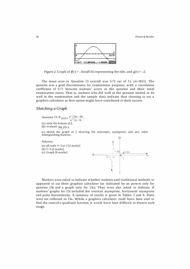
Question 13: If f (x) = x2 + 3x− 10

x2 + x − 6,

(a) state the domain of f,(b) evaluate

limx→2

f (x ) ,

(c) sketch the graph of f showing the intercepts, asymptotes and any otherdistinguishing features.

Solution:(a) all reals ≠ -3 or 2 [2 marks](b) 7/5 [2 marks](c) Graph [6 marks]

Markers were asked to indicate whether students used traditional methods orappeared to use their graphics calculator (as indicated by an answer only forquestion 13b and a graph only for 13c). They were also asked to indicate ifstudents’ graphs for 13c included the vertical asymptote, horizontal asymptoteand point discontinuity. A summary of results is given in Tables 5 and 6. Datawere not collected on 13a. While a graphics calculator could have been used tofind the roots of a quadratic function, it would have been difficult to discern suchusage.


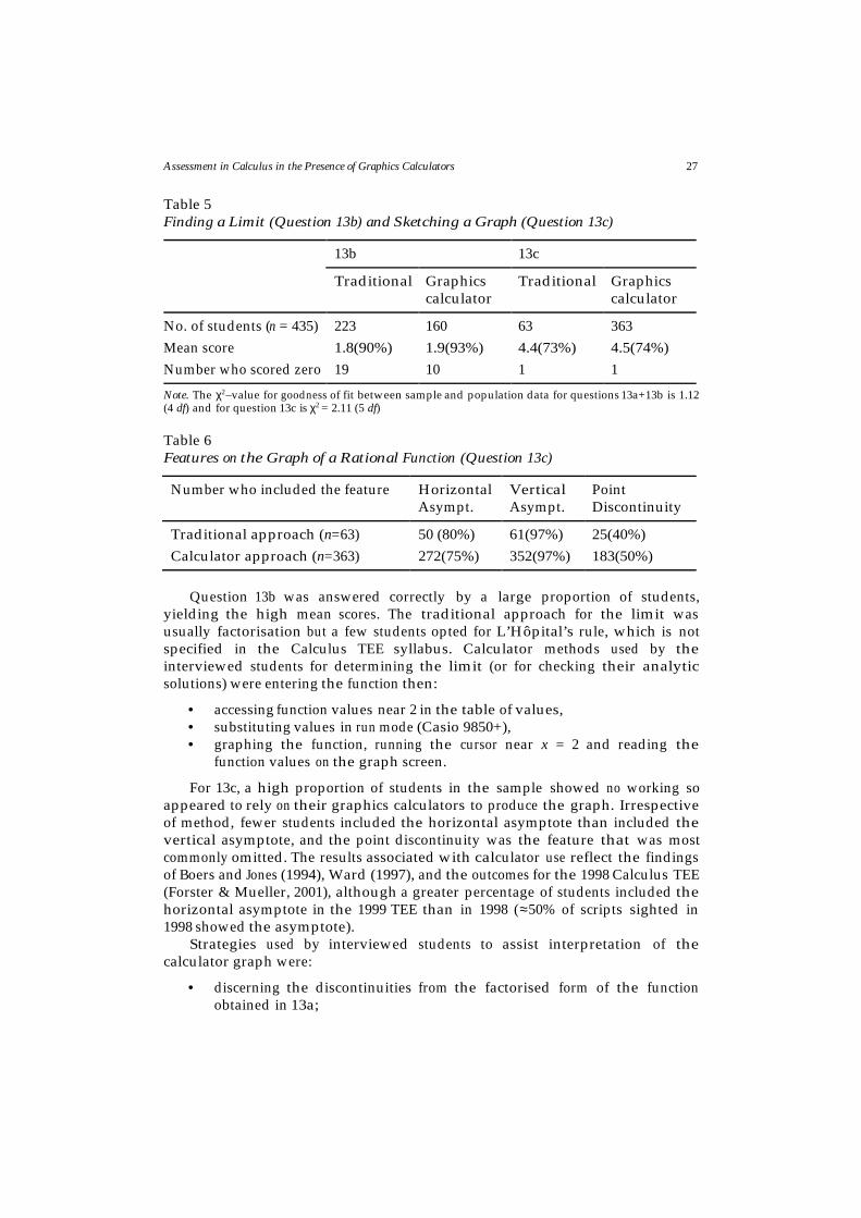
Table 5Finding a Limit (Question 13b) and Sketching a Graph (Question 13c)

13b 13c



No. of students (n = 435) 223 160 63 363Mean scoreNumber who scored zero

1.8(90%)19

1.9(93%)10

4.4(73%)1

4.5(74%)1

Note. The χ2–value for goodness of fit between sample and population data for questions 13a+13b is 1.12(4 df) and for question 13c is χ2 = 2.11 (5 df)

Table 6Features on the Graph of a Rational Function (Question 13c)

Number who included the feature HorizontalAsympt.

VerticalAsympt.

PointDiscontinuity

Traditional approach (n=63) 50 (80%) 61(97%) 25(40%)Calculator approach (n=363) 272(75%) 352(97%) 183(50%)

Question 13b was answered correctly by a large proportion of students,yielding the high mean scores. The traditional approach for the limit wasusually factorisation but a few students opted for L’Hôpital’s rule, which is notspecified in the Calculus TEE syllabus. Calculator methods used by theinterviewed students for determining the limit (or for checking their analyticsolutions) were entering the function then:

• accessing function values near 2 in the table of values,• substituting values in run mode (Casio 9850+),• graphing the function, running the cursor near x = 2 and reading the

function values on the graph screen.

For 13c, a high proportion of students in the sample showed no working soappeared to rely on their graphics calculators to produce the graph. Irrespectiveof method, fewer students included the horizontal asymptote than included thevertical asymptote, and the point discontinuity was the feature that was mostcommonly omitted. The results associated with calculator use reflect the findingsof Boers and Jones (1994), Ward (1997), and the outcomes for the 1998 Calculus TEE(Forster & Mueller, 2001), although a greater percentage of students included thehorizontal asymptote in the 1999 TEE than in 1998 (≈50% of scripts sighted in1998 showed the asymptote).

Strategies used by interviewed students to assist interpretation of thecalculator graph were:

• discerning the discontinuities from the factorised form of the functionobtained in 13a;


• being alert to the vertical asymptote and point discontinuity fromanswers to 13a and b;

• mentally substituting ±x into the function;• using the table of values—with x = 0 to evaluate the y intercept, with

x = 2 to check the discontinuity, and with large positive and negativenumbers to locate the horizontal asymptote;

• on the graph, using the root finding facility, observing the break in thegraph at x = 2, and using the trace facility to establish that the graphapproached y = 1.

Thus, interpretation of the graph was assisted by determination of thestructure from the algebraic form of the function; and by mental calculation,dynamic reading of the graph and procedures in the table of values. Some of theinterviewed students used one of these approaches to check the results of another.Bringing to bear the structural and operational understandings mediatedfavourably interpretation of the graph and omission to do so explains the non-identification of key features. The discretisation of the calculator graph meansfeatures are not always visible and necessitates that students predict them fromthe function expression. Other errors attributable to discretisation and to blindcopying of a calculator graph were stopping the branches of the curve withoutindicating asymptotic behaviour, and joining the branches of the curve. In copyingthe graph it is also important to clearly identify the features that have beennoticed. Some students drew the branches of the curve as approximatelyhorizontal but did not clearly identify the y = 1 asymptote and were penalised.

The mean mark for the population for parts 13a-b was 3.36 out of 4, n = 1981,and for 13c was 4.47 out of 6, n = 1907.

Generation and Interpretation of a Graph

Question 14: A particle is moving along a straight line that runs in an east-westdirection. Its position function s(t) at time t is given by

s(t) = t 2 + 1

t 4 + 1.

(a) Determine the velocity function of the particle.(b) The particle is moving in an easterly direction when the velocity is positive. Usethe graph of the velocity function to decide when the particle is moving in a westerlydirection.(c) Use the graph of the velocity function to determine the maximum speed of theparticle and when it is attained.(d) Calculate the position of the partic le at the time when the maximum speed isattained.

Solution:(a)

s = t2 + 1

t4 + 1, v = (t4 +1)2t − (t 2 +1)4t 3

(t4 + 1)2 = 2t − 2t 5 − 4t 3

(t4 + 1)2 [3 marks]

(b) t > 0.64 [2 marks](c) t = 1.095 (3 d.p.), speed = 1.045 (3 d.p.) [2 marks](d) s = 0.90 (2 d.p.) [1 mark]

Part marks for questions 14a-c were recorded for the sample of students (seeTable 7) and whether students drew a graph in support of their answers.


Table 7Finding a Derivative (Question 14a) and Interpreting a Graph (Question 14b-c)

14a 14b 14c

Students attempting the question (n = 435) 419 380 368Mean score 2.6 (88%) 1.3(63%) 1.2(59%)Number of students scoring zero 16 102 122

Note. The χ2–value for goodness of fit between sample and population data is χ2(7, N = 435) = 1.41 .

Students were more successful in question 14a, which involved differentiation(without technology), than in 14b and 14c. Written answers for 14b and c lackedalgebraic working, suggesting that students drew the required graph using theircalculators (see Figure 3). The graph would have been difficult to establishanalytically, so that graphical approaches on a calculator were effectivelyforced. Mistakes in the calculation of the derivative were followed through inthe marking, so they did not impact greatly on the results for 14b and 14c. Thehigh number of students in the sample scoring zero and the low average marksassociated with these part questions can therefore be attributed largely todifficulties with interpreting the questions and with obtaining an adequategraphical display and interpreting it.

Figure 3. Graph of the velocity function.

Student errors in 14b were giving the answer as:

• t < 0.64, which is consistent with knowing that the direction of travelchanges at v = 0, but incorrectly assumes that westerly travel involvesmoving to the left on the graph;

• 0.64 < t < 1, which correctly recognises that the section below thehorizontal axis represents travel in the westerly direction but incorrectlyassumes that the relative minimum turning point is where the particleturns round;

• t = 0.64, which implies a misinterpretation of the question.

Recognising that the root of the velocity function was needed was lessproblematic than determining the appropriate interval. Interviewed studentsindicated that they used built-in capabilities of their calculators to determinethe root.

In relation to the maximum speed for 14c errors were:


f(t )

t

1

2

-1

-2

π

(1·17, 1·45)

• to give maximum velocity (the highest point on the graph) for maximumspeed,

• to give the speed at the minimum point but write it incorrectly as anegative quantity, and

• to omit the time.

Interviewed students again indicated that they used built-in capabilities ontheir calculators to determine the time and speed.

From a theoretical viewpoint, the graph allows the functional relationshipto be seen as a whole, but its structure does not bear any likeness to the motion itsignifies. Therefore, literal interpretation of the structure is inappropriate (thatwest is left, and the particle turns at the turning point), yet, such interpretationexplains the mis-identification of the interval in 14b. Checking the negativity ofvelocity function values at a few positions, in other words, exploring the detail ofthe graph, which calls on operational understanding, could increase thelikelihood of a correct choice of the interval. Students that we interviewedtypically just “knew” movement was west below the x axis. Literal interpretationalso explains the answer of maximum velocity in 14c.

The mean score for the question for the entire population was 5.50 out of 8, n =1891.

Testing for Continuity and Graphical Solution of a Non-linearEquation

Question 20: The function f is defined by f (t) = sin(tx) dx

0

2

∫ .

(a) Show that

f(t)=1− cos(2t)

tfort≠ 0

0 fort = 0

(b) Determine limt →0

f(t) , justifying your answer.

(c) Is f continuous at t = 0? Justify your answer.(d) Sketch the graph of f.(e) What is the least integer value of K such that all solutions of the equationf(t) = 0.25 are contained in the interval [0, K]?(f) How many values of t are there with f(t)=0.25?

Solutions: For economy of space, solutions for (a) and (b) are omitted. For (b) thelimit is zero and methods students adopted are described below.(c) f(t) = 0 =

limt →0

f(t) ∴ f(t) is continuous a t = 0 [2 marks]

(d) Graph [4 marks](e) K = 8 [1 mark](f) 6 solutions [2 marks]


Markers recorded part marks for question 20b and the method (traditional,table of values, or a graph); and part marks for 20d and 20f, which required theuse of the calculator due to the non-routine nature of the function (see Table 8).

Few students conclusively established the value of the piecewise-definedfunction at x = 0 and errors from 20a and 20b flowed into 20c. Of the students whosemethod was recorded for the limit in 20b, about two thirds drew on standardapproaches for limits including application of L’Hôpital’s rule and theproperties of trigonometric limits. Some interviewed students noted that thevalue of the limit was a known fact. The alternatives were a table of values orgraph, which potentially were both graphics calculator assisted. Mean scoreswere noticeably higher for those students who used these approaches. However,errors were:

• some students did not provide sufficiently many values in their table toadequately establish the limiting behaviour, an omission also noted forthe 1998 Calculus TEE (Forster & Mueller, 2001),

• students correctly stated the limit of the function as t approached zerofrom above and below zero, but incorrectly included f(0) = 0 in theirjustification,

• isolated instances of graphs with asymptotic behaviour at t = 0, whichwas consistent with students keying the function 1− cos(2t)/ t into theircalculators.

Table 8Evaluating a Limit (20b), Sketching a Graph (20d) and Interpreting a Graph (20f)

20b 20d 20f

Traditional Table Graph

No. of students (n = 435) 182 58 35 312 271Mean score 1.7(58%) 2.5(83%) 2.1(70%) 2.3(58%) 0.8(40%)

Note. The χ2–value for goodness of fit between sample and population data is χ2(16, N = 435) = 13.15 .

The earlier discussion on limits in the interpretative framework is pertinenthere. The correct application of traditional symbolic procedures does notnecessarily indicate operational understanding of the limit concept, that is,understanding of limiting behaviour. Too few values in a table implies, at best,weak operational understanding, as does the inclusion of f (0) = 0 with thegraphical approach: a sufficient procedure with the graph is gauging functionvalues on either side of t = 0. Besides being unnecessary, stating f (0) = 0 indicatesmisinterpretation of the structure of the function. The function (1− cos 2t)/ t has apoint discontinuity at t = 0. This is another instance where predicting features ofthe graph from the algebraic expression is desirable because the discontinuitywould not necessarily be evident on calculator graphs. Misconstruing that f(0)exists affected answers for 20c.

In 20d, calculator graphing was effectively forced due to the nature of the


function. Graphs typically lacked coordinates of a point to set the scales andlacked scales on the axes, which is attributable to there being no scales on somecalculator graphs. In 20e, the interviewed students deduced the interval by:

• using the extremum function on the graph to find the relative maximavalues,

• tracing along the curve with the cursor and relying on the function valueoutputs,

• graphing f(x) = 0.25 and using the point of intersection capability to checkthe allowable t values.

A widespread error in 20e in written solutions was failure to round to aninteger. Only 58% of candidates in the sample answered 20f and less than half ofthem gave 6 for the answer. The errors and omissions explain the low mean scoresfor questions 20d and 20f. The mean result for the question as a whole was a low7.05 out 16, n = 1749. Question 20 was the last question in the examination paperand, judging by interview comments, many students were pressed for time.

In summary, we have described how students might have utilised theirgraphics calculators in answering seven examination questions, the associatedmean scores, errors that were made, and some aspects of the understanding calledupon. We finish this section of the paper with an overview of the apparentextent of calculator use and success associated with the use. For the evaluation ofan integral where calculator-use was necessary, results indicate that a significantnumber of students did not recognise to use the tool or did not use it correctly(Question 6). Only 45% of all candidates scored full marks. Where calculator-usewas optional for integrals, the high majority of students in the sample chose itand, in Question 7, 70% of them scored full marks. In the other (Question 8), 64%correctly used the calculator to evaluate the integral that they had. Thecomplexity of the expressions in Questions 6 and 8 is relevant to the lower results.The mean marks achieved with hand and calculator evaluations do not indicatea clear pattern of inferior or superior performance with either method (see Tables2 and 3).

Use of graphs, tables of values, and the solve function on the calculators isoften not distinguishable in written answers, so results for them are consideredtogether and summarised in Table 9. Use of the calculators was forced in questions14b and c, and 20d and f because of the complex functions.

Where the use of calculators was optional, the majority of students in thesample appeared to rely on them when a graph was required (Question 13).Otherwise, less than half the written answers were consistent with a calculatormethod, although students might have used the technology for checking. Theparticularly small number of students choosing the calculator in Question 7 wasattributable to exact values being stipulated, and they scored, on average, lowerthan students who presented analytic working.


Table 9Results by Question when Choosing Graphs, Table of Values or the Solve Facility

Application No. of students (n = 435) Mean Score %

Graphicscalculator


Traditional

7b Obtaining the co-ordinates of amaximum stationary point.

99 311 76 81

12c Solving a trigonometric equationinvolving the tide.

123 151 75 64

13b Evaluating a limit. 160 223 93 90

13c Graphing a rational function. 363 63 74 73

14b Solving for times when a particlewas travelling West.

380 n.a. 63 n.a.

14c Identifying maximum speed. 368 n.a. 59 n.a.

20b Evaluating a limit. 93 182 78 58

20d Graphing a trigonometricfunction.

312 n.a. 58 n.a.

20f Finding the no. of solutions tosimultaneous equations.

271 n.a. 40 n.a.

The difference in percentage scores is highest in favour of calculator users onthe questions that asked for a departure time (Question 12c) and a trigonometriclimit (Question 20b). The difference in marks was not substantial for Question 12c(0.3 marks out of 5), but contributed to Question 12 as a whole being one of the bestdiscriminators on the examination. The tabular approach to the limit in Question20b resulted in the greatest advantage (see Table 8) and students using the tablescored on average 0.8 marks out of 3 more than the traditional group.

The lowest mean scores recorded for calculator users were on Questions 20dand f, but students’ running out of time might have affected performance on themmore adversely than on other questions. The relatively low scores on Questions14b and c are explained by inappropriate literal interpretation of the graph.However, misinterpretation of graphs of derivative functions is known to bewidespread (e.g., Hale, 2000) and is not limited to calculator-produced graphs.

ConclusionIn this paper we have described students’ performance in relation to graphics

calculator use on selected questions from the 1999 Calculus TEE. Based on themethods that the interviewed students articulated, we have identified howgraphs can assist problem-solving because they display the structure of functions.For example, a periodic structure (Question 12) and the existence of turning points(in Questions 7, 12, 14 and 20). Importantly, though, domains and scales need to becarefully selected so that features are displayed. Optimal selection can involve


restricting the domain to values specified in the question (Question 12), and atrigonometric rather than decimal scale (Question 7). Even so, some featuresmight not be visible, the structure displayed might be inconsistent withconventional graphing, and the structure might bear little resemblance to thephenomena it is representing. Examples are, respectively, point discontinuities(Questions 13 and 20), branches of a curve stopping on asymptotes (Question 13),and spatial relationships on a velocity time graph (Question 14). Therefore,exploratory work is recommended.

We established that exploration meant prediction of graphical features fromthe function expression and previous part questions; reading along the branches ofa graph and judging the function values; and accessing the table of values todetermine or check function values. Thus, ideally, structural understanding (offunctions as wholes), operational understanding (of the ways function valuesdepend on x) and procedures for accessing function values are brought to bear ininterpreting the graphs; and contexts need to be accommodated.

Specifically, operational understanding was elicited and incompleteunderstanding revealed by some (relatively few) students in their calculator-based determination and justification of a limit (Question 20). Students’ scoresindicate the demands of graphical interpretation were particularly high withthe velocity function (Question 14), but difficulty with interpreting graphs of aderivative function is not limited to calculator graphs.

Once the graphical features that are relevant to an examination questionhave been determined, students can use the automated calculation facilities onthe calculator to produce numerical answers. The automation is compensation forthe demanding work of graphical interpretation. The interviewed studentsindicated use of automated facilities for roots (Question 14), coordinates ofturning points (Questions 7, 14 and 20), and coordinates of points of intersection(Questions 12 and 20). The table of values and trace facility were also accessed.

A final step in the graphical solution is transcription of the graph or thenumerical values from the graph, onto the examination script. Attention neededto be given (and was not always) to clearly identifying graphical features(Question 13); to compensating for limitations of the calculator graph (by, forexample, not joining branches across a vertical asymptote) (Question 13); toproviding scales on the axes (Question 20); and to converting decimals from thecalculator to exact values (Question 7).

Implications for teaching are that procedures associated with graphicalsolutions need to be the subject of instruction. These include procedures for (a)setting up the calculator for an adequate graph, (b) enhancing graphicalinterpretation, (c) obtaining numerical outputs and (d) ensuring written answersare adequate. In particular, the moving between the different sources ofinformation while interpreting the graph might not fall into our conventionaldefinition of algorithmic, but is a learnt skill that needs to be explicitlyaddressed in class. In other words, different operational and structuralinterpretations of graphs and other symbolic forms need to be encountered in classand students encouraged to integrate them. As well, operational views need to berevisited so that pseudo-structural thinking (Sfard & Linchevski, 1994), theapplication of procedures without knowing the true nature of the concept to


which they relate, is avoided.If a calculator solution is attempted it is also important to know the syntax

required in relation to entering function expressions (Question 20) and more so inrelation to complex integral expressions (Questions 6 and 8). Our inquiry hasuncovered this as a problematic area for some students. Boers and Jones (1994) alsofound incorrect entry a problem. Other sites for error were not having thecalculator set to the appropriate angle mode (Questions 6 and 7), and use of thesolve facility (Questions 7 and 12). A limitation of the numerical solve is thatthe solution obtained is nearest to an estimate that the student enters. A visualcheck with the linked graph is recommended, or use of the graph from the start.These aspects of calculator use also have implications for teaching.

Implications of our inquiry for assessment are that an awareness of thedemands of graphical interpretation and of likely misinterpretation needs to bebrought to the setting of questions. In addition, a balance between opportunitiesfor visual, empirical approaches and analytic methods needs to be built intoexamination papers. We say this in view of the increased role for diagrams andgraphs in the Calculus TEE since the introduction of graphics calculators (Mueller& Forster, 2000), and in view of indications of superior performance by girls onquestions requiring analytic solutions and by boys on questions requiring complexgraphical interpretation (Forster & Mueller, in press). A question for research iswhat balance is desirable, and an assessment issue is why do examinationquestions ask for exact values if use of the calculators is expected and valued?

The subjective nature of the sample data leads us to be cautious in reachingfirm conclusions on the extent of calculator usage. However, in relation to optionaluse, when a question required a graph (Question 13) or the evaluation of anintegral (Questions 7 and 8), the high majority of students opted for calculatoruse. In other instances when calculator usage was optional, less than half thestudents in the sample seemed to choose it, but for those that did there seemed tobe most advantage in using the table of values for the evaluation of a difficultlimit (Question 20).

Our analysis has illustrated the changed nature of TEE Calculus in WesternAustralia following the introduction of graphics calculators and has developedthe theme that students need to have strategies to check graphical, empiricalsolutions. It also seems time to clarify what it is that we want Year 12 Calculusstudents to know in the presence of the technology.

ReferencesAlguire, H., & Forster, P. A. (1999). Promoting mathematical understanding through the use of

graphics calculators. Proceedings of the Australian Curriculum, Assessment andCertification Authorities Conference (pp. 131-144). Perth: Curriculum Council..

Anderson, M., Bloom, L., Mueller, U., & Pedler, P. (1997). Graphics calculators: Someimplications for course content and examination. Paper presented at the third AsianTechnology Conference in Mathematics. Available: http://www.runet.edu/~atcm/atcm97.html

Berger, M. (1998). Graphics calculators: An interpretative framework. For the Learning ofMathematics, 18 (2), 13-20.

Boers, M. A. M., & Jones, P. L. (1994). Students’ use of graphics calculators underexamination conditions. International Journal of Mathematics Education in Science andTechnology, 25 (4), 491-516.

Brown, R., & Neilson, B. (2001). What algebra is required in “high stakes” system wide

http://www.runet.edu/~atcm/


assessment? A comparison of three systems. In H. Chick, K. Stacey, J. Vincent & J. Vincent(Eds.), The future of teaching and learning of algebra, Proceedings of the 12th ICME StudyConference (pp. 128-135). Melbourne: University of Melbourne..

Forster, P. A., & Mueller, U. (2001). Outcomes and implications of students’ use of graphicscalculators in the public examination of calculus. International Journal of MathematicalEducation in Science and Technology, 32 (1), 37-52.

Forster, P. A., & Mueller, U. (in press). What effect does the introduction of graphicscalculators have on the performance of boys and girls in assessment of tertiary entrancecalculus? International Journal of Mathematical Education in Science and Technology.

Forster, P. A., & Taylor, P. C. (2000). A multiple perspective analysis of learning in thepresence of technology. Educational Studies in Mathematics, 42 (1), 35-59.

Gray, E. M., & Tall, D. O. (1994). Duality, ambiguity, and flexibility: A “proceptual” view ofsimple arithmetic. Journal for Research in Mathematics Education, 25 , 116-146.

Hale, P. (2000). Kinematics and graphs: Students’ difficulties and CBLs. Mathematics Teacher,93 (5), 414-417.

Hiebert, J., & Carpenter, T. P. (1992). Learning and teaching with understanding. In D. A.Grouws (Ed.), Handbook of research in mathematics teaching and learning (pp. 65-97).New York: Macmillan.

Hollar, J. C., & Norwood, K. (1999). The effects of a graphing-approach intermediate algebracurriculum on students’ understanding of function. Journal for Research in MathematicsEducation, 30 (2), 220-226.

Jones, P., & McCrae, B. (1996). Assessing the impact of graphics calculators on mathematicsexaminations. In P. Clarkson (Ed.), Technology in mathematics education (Proceedings ofthe 19th annual conference of the Mathematics Education Research Group ofAustralasia, pp. 306-313). Melbourne: MERGA.

Kemp, M., Kissane, B., & Bradley, J. (1996). Graphics calculators use in examinations:Accident or design? Australian Senior Mathematics Journal, 10 (1), 33-50.

Mueller, U., & Forster, P. A. (2000). A comparative analysis of the 1996-1999 Calculus TEEpapers. In J. Bana & A. Chapman (Eds.), Mathematics education beyond 2000 (Proceedingsof the twenty-third annual conference of the Mathematics Education Group ofAustralasia, Perth, pp. 465-473). Sydney: MERGA.

Nesher, P. (1986). Are mathematical understanding and algorithmic performance related? Forthe Learning of Mathematics, 6(3), 2-9.

Schwarz, B. B., & Hershkowitz, R. (1999). Prototypes: Brakes or levers in learning thefunction concept? The role of computer tools. Journal for Research in MathematicsEducation, 30 (4), 362-389.

Senk, S. L. Beckmann, C. E., Thompson, D. R. (1997). Assessment and grading in high schoolmathematics classrooms. Journal for Research in Mathematics Education, 28 (2), 187-215.

Sfard, A. (1991). On the dual nature of mathematical conceptions: Reflections on processesand objects as different sides of the same coin. Educational Studies in Mathematics, 22, 1-36.

Sfard, A., & Linchevski, L. (1994). The gains and pitfalls of reification – the case of algebra.Educational Studies in Mathematics, 26 , 191-228.

Tall, D. O., & Thomas, M. O. J. (1991). Encouraging versatile thinking in algebra using thecomputer. Educational Studies in Mathematics, 22 , 125-147.

Ward, R. A. (1997). An investigation of scaling issues and graphing-calculator associatedmisconceptions among high school students. (Doctoral dissertation, University ofVirginia, 1997). Dissertations Abstracts International, 58/06, 1.

AuthorsPatricia A. Forster, Faculty of Community Services, Education and Social Sciences, EdithCowan University, 2 Bradford Street, Mt Lawley, Western Australia 6050. E-mail:<[email protected]>

Ute Mueller, School of Engineering and Mathematics, Edith Cowan University, 100Joondalup Drive, Joondalup, Western Australia 6027. E-mail: <[email protected]>

mailto:[email protected]

mailto:[email protected]

Documents

Assessment in Calculus in the Presence of Graphics Calculators · Assessment in Calculus in the Presence of Graphics Calculators ... appropriate to the task at hand, ... can be represented