Assessing the Inﬂuence of Regional SST Modes on the Winter

Assessing the Influence of Regional SST Modes on the Winter Temperature in China:The Effect of Tropical Pacific and Atlantic

ZHIHONG JIANG AND HAO YANG

Key Laboratory of Meteorological Disaster, Nanjing University of Information Science and Technology,

Ministry of Education, Nanjing, China

ZHENGYU LIU

Center for Climatic Research, University of Wisconsin—Madison, Wisconsin

YANZHU WU

Meteorological Bureau of Suzhou City, Suzhou, China

NA WEN

Key Laboratory of Meteorological Disaster, Nanjing University of Information Science and Technology,

Ministry of Education, Nanjing, China

(Manuscript received 27 November 2012, in final form 6 September 2013)

ABSTRACT

This study investigates the influence of different sea surface temperature (SST) modes on the winter

temperature in China using the generalized equilibrium feedback assessment (GEFA). It is found that the

second EOF mode of winter temperature in China during 1958–2010 shows a typical northeast–southwest

(NE–SW) pattern, which is a major spatial mode of Chinese winter temperature at interannual scales. The

winter temperature of the NE–SW pattern is forced mainly by SSTmodes in the tropical Pacific and Atlantic.

For 2009/10, the tropical Pacific El Ni~no mode and tropical Atlantic tripole mode have the largest contri-

bution to the response. The physical mechanism of the cold northeast–warm southwest (CNE–WSW) pattern

is also explained in terms of GEFA of the responses of the atmospheric circulation. The northerly flow at the

low level transports cold air to northern and northeastern China, resulting in a lower temperature there.

Meanwhile, the anomaly meridional wind advects warm air from the southern oceans to southwestern China,

leading to warming there.

1. Introduction

With the background global warming, the anomalous

winter air temperature has received widespread con-

cern in recent years (e.g., Wang and Zhang 2002; Yang

et al. 2007; Lin and Wu 2012; Jiang et al. 2012). Espe-

cially, extreme climate events in China have received

increasing attention during the past few years due to

their frequent occurrences (e.g., Wu et al. 2010; Chen

et al. 2010; Jiang et al. 2011;Ma et al. 2012). For instance,

northern China witnessed cold winter with heavy snow

disasters in 2009/10, during which Xinjiang Province

experienced the most serious damage in the last five

decades, while anomalous warming and drought oc-

curred over the southwest. In 2008 (January–February),

south China experienced continuous low temperature,

accompanied by themost severe large range of continuous

low temperature freezing rain and snowstorms in the last

50 years, leading to huge property losses and hundreds of

human lives (e.g., Hong and Li 2009; Wu et al. 2010).

In the meantime, our understanding and prediction

skill of these extreme events remain limited. Pu et al.

(2007) showed that the two basic spatial patterns of air

temperature changes over China are characterized by

Corresponding author address: Zhihong Jiang, Key Laboratory

of Meteorological Disaster of Ministry of Education, Nanjing Uni-

versity of Information Science and Technology, 219 Ningliu Rd.,

Nanjing, China.

E-mail: [email protected]

868 JOURNAL OF CL IMATE VOLUME 27

DOI: 10.1175/JCLI-D-12-00847.1

� 2014 American Meteorological SocietyUnauthenticated | Downloaded 10/25/21 11:32 AM UTC

mailto:[email protected]

the empirical orthogonal function (EOF) modes, the

EOF1 representing a consistent change in eastern China

and EOF2 representing opposite changes between north-

eastern and southwestern China [northeast–southwest

(NE–SW) pattern]. It was further shown that the two

basic spatial patterns above are stable in different pe-

riods. However, it has remained unclear what caused

the change of these temperature patterns. In particular,

it has remained unclear how the abnormal winter tem-

perature in China responds to global oceans. The impact

of SST on Chinese winter temperature is receiving in-

creasing attention. So far, the central and eastern equa-

torial Pacific SST has received the most attention. Many

studies suggest that El Ni~no events give rise to cold

northeast–warm southwest (CNE–WSW) pattern in

China (e.g., Wang et al. 2000; Chen et al. 2001). Ding

et al. (2008) suggested that the strong La Ni~na event in

the 2007/08 winter provides a climate background for

the invasion of cold air into southern China, and the

persistence of circulation anomalies over the Eurasian

continent is the direct cause of the snowstorms. Wang

et al. (2010) found that the East Asian (EA) winter mon-

soon (EAWM) variability are different between the ex-

tratropical and tropical EA. El Ni~no–Southern Oscillation

(ENSO), snow cover over northeastern Siberia, and SSTof

the North Atlantic and tropical Indian Oceans have been

suggested to be the major factors impacting EAWM.

One challenge in previous observational studies is to

isolate the atmospheric response to a specific oceanic

variability mode. This is because the atmospheric re-

sponse at a specific time usually consists of the responses

to multiple concurrent SST forcings (Klein et al. 1999;

Newman et al. 2003; Lau et al. 2006). Our study here

is an attempt to addresses the questions: How do SST

anomalies (SSTAs) impact the temperature variation in

winter over China synthetically? How much does each

SST mode contribute to the temperature anomaly?

Frankignoul et al. (1998) proposed a simple univariate

statistical method, later called the equilibrium feedback

assessment (EFA) (Liu and Wen 2008), for the assess-

ment of climate feedback. This method has now been

extended to the multivariate case as the generalized

equilibrium feedback assessment (GEFA) method (Liu

et al. 2008; Liu and Wen 2008). Using the GEFAmethod,

Wen et al. (2010) investigated the impacts of global SST

variability modes on geopotential height (GPH) in ob-

servations and showed that GEFA is able to distinguish

the impacts fromdifferent SSTmodes in different oceans.

Zhong et al. (2011) presented a comprehensive assess-

ment of the observed influence of the global ocean on

U.S. precipitation variability using the method of GEFA.

However, no relevant analysis has yet been conducted

on the climate variability in China.

Here, we will assess the impact of SST on winter

temperature in China in the observation using GEFA.

This paper is arranged as follows. The GEFA method is

first reviewed and the observational data are described

in section 2. Section 3 describes the characteristic win-

ter temperature response pattern in China, the NE–SW

pattern, in composite analysis and EOF analysis. The

SST impact on the air temperature response pattern and

the physical mechanism are further studied in sections 4

and 5, respectively. The last section summarizes the

major findings.

2. Data and method

a. Data

The major datasets used in this study include 1)

monthly-mean surface air temperature data at 160 gauge

stations across China from the China Meteorological

Administration, and 2) monthly-mean SST, GPH, sea

level pressure (SLP), and wind fields data, gridded at

2.58 3 2.58 resolution taken from the National Centers

for Environmental Prediction–National Center for At-

mosphericResearch (NCEP–NCAR)GlobalReanalysis 1

(NCEP-1) data for the 1958–2010 period (available on-

line at http://www.cdc.noaa.gov/cdc/data.ncep.reanalysis.

derived.html). Here, winter refers toDecember–February.

b. Generalized equilibrium feedback assessment

GEFA is a multivariate generalization of the univar-

iate EFA (Frankignoul et al. 1998; Liu et al. 2006;

Notaro et al. 2006a) to facilitate distinguishing the im-

pacts by interrelated oceanic forcings. A full formula-

tion of GEFA has been demonstrated in Liu et al. (2008)

and Liu and Wen (2008). For the convenience of the

readers, we will briefly discuss GEFA here.

Assume the atmospheric variability at month t X(t)

consists of a stochastic part associated with the atmo-

spheric internal variability N(t) and a SST-forced part

B 3 T(t), such that

Xt 5B3Tt 1Nt (1)

or

xi(t)5 �J

j51

bijTj(t)1ni(t) . (2)

The SST field Tt consists of j points, representing j SST

indices. Here, B is the response sensitivity matrix with

components bij judging the impact of the jth SST index

on the temperature variability fields. Simultaneous as-

sociation of SSTs and atmospheric variability primarily

15 JANUARY 2014 J I ANG ET AL . 869

Unauthenticated | Downloaded 10/25/21 11:32 AM UTC

http://www.cdc.noaa.gov/cdc/data.ncep.reanalysis.derived.html

http://www.cdc.noaa.gov/cdc/data.ncep.reanalysis.derived.html

reflects the atmosphere driving the ocean, requiring that

calculations aimed at quantifying oceanic feedbacks to

the atmosphere use data with the atmosphere lagging the

ocean (Frankignoul et al. 1998; Czaja and Frankignoul

2002). Therefore, B is derived with atmosphere-lagged

covariances as

B(t)5CXT(t)C21TT(t) , (3)

where t is a SST lead time that is longer than the

damping time scale of the atmosphere, CXT(t) is the

lagged cross-covariance matrix between atmospheric

variability and SST, and CTT(t) is the autocovariance

matrix of SST. Discrimination of the impacts by in-

terrelated SST forcings now becomes effortless by sin-

gling out each component bij. Here, t is chosen to be

1 month in this study, as t 5 2 months tends to yield

similar results (Wen et al. 2010). The significant test of

B is performed using the Monte Carlo bootstrap ap-

proach (Czaja and Frankignoul 2002). The computation

of B is repeated 500 times, each using randomly scram-

bled atmospheric time series. The atmospheric season-

ality is retained, as only the order of the years is changed,

not that of the months.

3. GEFA in the EOF space

a. The definition of NE–SW pattern

To discriminate the variation characteristics of winter

air temperature, we perform EOF analysis of the winter-

mean temperature over China from 1958/59 to 2009/10

(Wei 2007). The first EOF mode (explaining 55% of the

total variance) mainly reflects the consistent warming

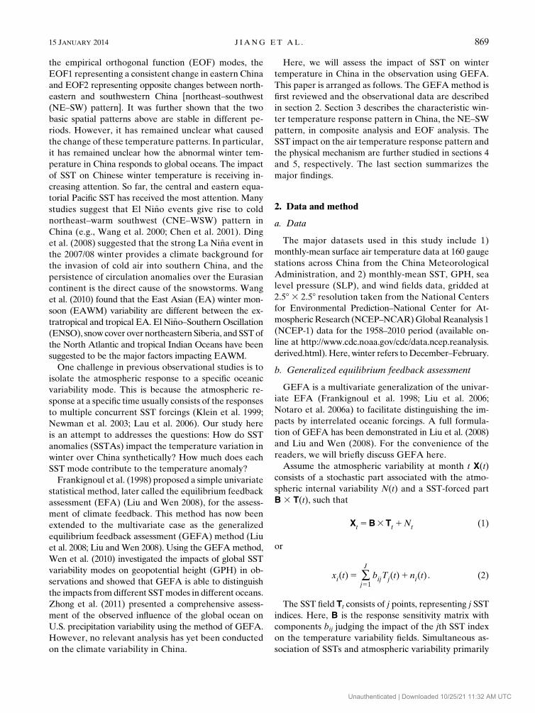
trend (figure omitted). The second EOF mode (explain-

ing 14% of the total variance) in Fig. 1a reflects a dipole

temperature anomaly between northeastern China and

southwestern China, which will be called the pattern of

NE–SW. In particular, the positive center lies in south-

western China, reaching above 18C, while the negative

center appears in the northeast area, with 228C. Thecorresponding principal components (PCs; Fig. 1b) show

clear interannual variability. According to the first and

second PCs (PC1 and PC2; Fig. 1b), years with PC1, 0.5

standard deviation (s5 0.5) and PC2. 1.5 (s5 1.5) are

defined as the NE–SW positive phases (CNE–WSW)

years. In contrast, years with PC1 lower than 0.5, and

PC2 less than21.5, are defined as the NE–SW negative

phases (warm northeast–cold southwest) years. Ac-

cording to the definition, the NE–SW positive phases

years include 1965/66, 2000/01, and 2009/10. The neg-

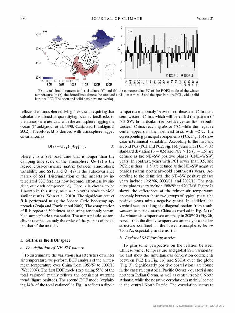
ative phases years include 1988/89 and 2007/08. Figure 2a

shows the differences of the winter air temperature

anomaly between these two groups of typical years (the

positive years minus negative years). In addition, the

vertical section (along the diagonal section from south-

western to northeastern China as marked in Fig. 2a) of

the winter air temperature anomaly in 2009/10 (Fig. 2b)

reveals that the dipole temperature anomaly is a shallow

structure confined in the lower atmosphere, below

700 hPa, especially in the north.

b. Regional SST forcing modes

To gain some perspective on the relation between

Chinese winter temperature and global SST variability,

we first show the simultaneous correlation coefficients

between PC2 (in Fig. 1b) and SSTA over the globe

(Fig. 3). Significantly positive correlations are found

in the eastern equatorial Pacific Ocean, equatorial and

northern Indian Ocean, as well as central tropical North

Atlantic, while the negative correlation is mainly located

in the central North Pacific. The correlation seems to

FIG. 1. (a) Spatial pattern (color shadings, 8C) and (b) the corresponding PC of the EOF2 mode of the winter

temperature. In (b), the dotted lines denote the standard deviation s561.5 and the open bars are PC1 , while solid

bars are PC2. The open and solid bars have no overlap.



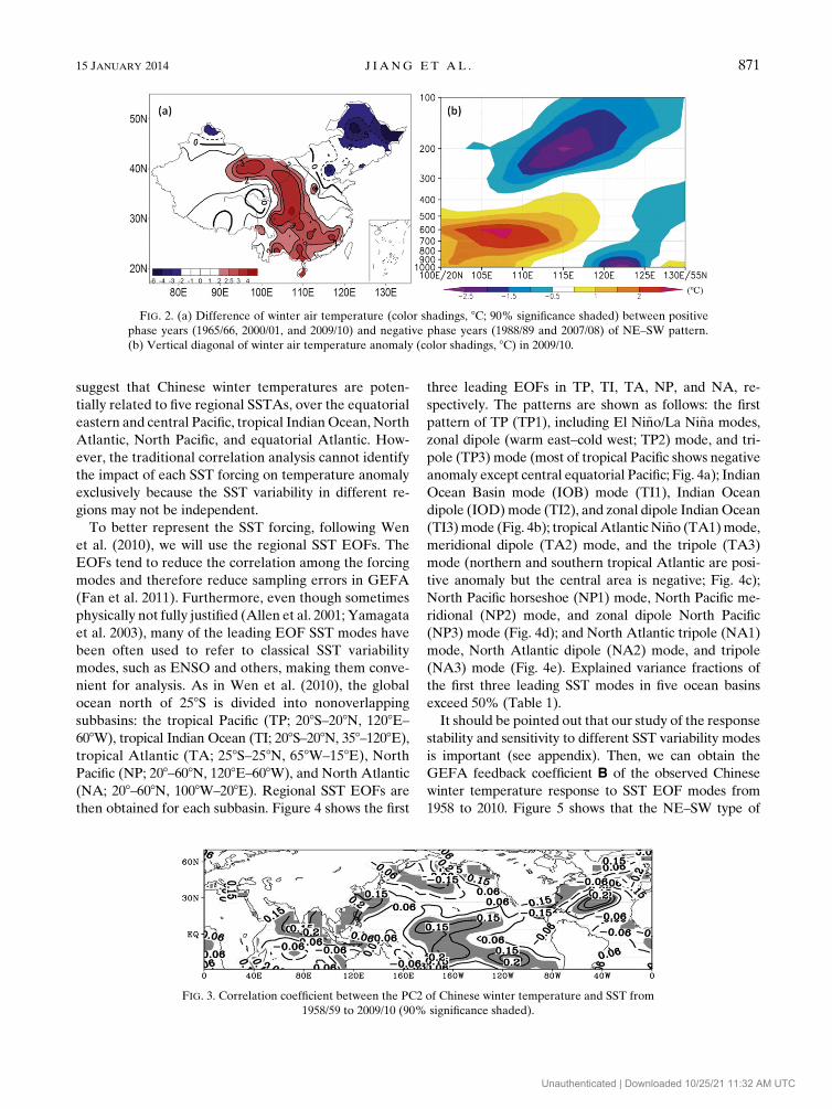
suggest that Chinese winter temperatures are poten-

tially related to five regional SSTAs, over the equatorial

eastern and central Pacific, tropical IndianOcean, North

Atlantic, North Pacific, and equatorial Atlantic. How-

ever, the traditional correlation analysis cannot identify

the impact of each SST forcing on temperature anomaly

exclusively because the SST variability in different re-

gions may not be independent.

To better represent the SST forcing, following Wen

et al. (2010), we will use the regional SST EOFs. The

EOFs tend to reduce the correlation among the forcing

modes and therefore reduce sampling errors in GEFA

(Fan et al. 2011). Furthermore, even though sometimes

physically not fully justified (Allen et al. 2001; Yamagata

et al. 2003), many of the leading EOF SST modes have

been often used to refer to classical SST variability

modes, such as ENSO and others, making them conve-

nient for analysis. As in Wen et al. (2010), the global

ocean north of 258S is divided into nonoverlapping

subbasins: the tropical Pacific (TP; 208S–208N, 1208E–608W), tropical Indian Ocean (TI; 208S–208N, 358–1208E),tropical Atlantic (TA; 258S–258N, 658W–158E), North

Pacific (NP; 208–608N, 1208E–608W), and North Atlantic

(NA; 208–608N, 1008W–208E). Regional SST EOFs are

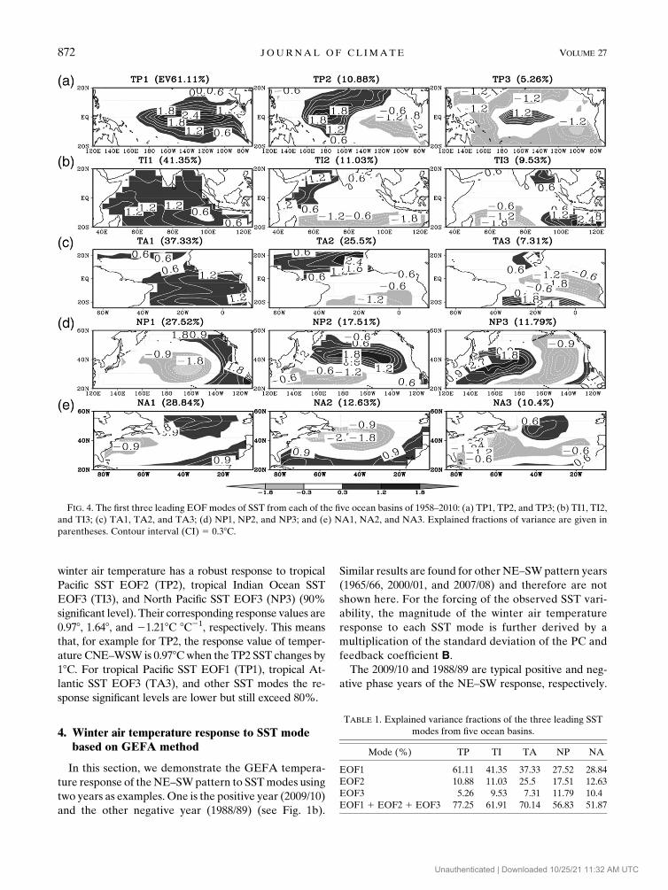
then obtained for each subbasin. Figure 4 shows the first

three leading EOFs in TP, TI, TA, NP, and NA, re-

spectively. The patterns are shown as follows: the first

pattern of TP (TP1), including El Ni~no/La Ni~na modes,

zonal dipole (warm east–cold west; TP2) mode, and tri-

pole (TP3) mode (most of tropical Pacific shows negative

anomaly except central equatorial Pacific; Fig. 4a); Indian

Ocean Basin mode (IOB) mode (TI1), Indian Ocean

dipole (IOD)mode (TI2), and zonal dipole IndianOcean

(TI3)mode (Fig. 4b); tropicalAtlanticNi~no (TA1)mode,

meridional dipole (TA2) mode, and the tripole (TA3)

mode (northern and southern tropical Atlantic are posi-

tive anomaly but the central area is negative; Fig. 4c);

North Pacific horseshoe (NP1) mode, North Pacific me-

ridional (NP2) mode, and zonal dipole North Pacific

(NP3) mode (Fig. 4d); and North Atlantic tripole (NA1)

mode, North Atlantic dipole (NA2) mode, and tripole

(NA3) mode (Fig. 4e). Explained variance fractions of

the first three leading SST modes in five ocean basins

exceed 50% (Table 1).

It should be pointed out that our study of the response

stability and sensitivity to different SST variability modes

is important (see appendix). Then, we can obtain the

GEFA feedback coefficient B of the observed Chinese

winter temperature response to SST EOF modes from

1958 to 2010. Figure 5 shows that the NE–SW type of

FIG. 2. (a) Difference of winter air temperature (color shadings, 8C; 90% significance shaded) between positive

phase years (1965/66, 2000/01, and 2009/10) and negative phase years (1988/89 and 2007/08) of NE–SW pattern.

(b) Vertical diagonal of winter air temperature anomaly (color shadings, 8C) in 2009/10.

FIG. 3. Correlation coefficient between the PC2 of Chinese winter temperature and SST from

1958/59 to 2009/10 (90% significance shaded).



winter air temperature has a robust response to tropical

Pacific SST EOF2 (TP2), tropical Indian Ocean SST

EOF3 (TI3), and North Pacific SST EOF3 (NP3) (90%

significant level). Their corresponding response values are

0.978, 1.648, and 21.218C 8C21, respectively. This means

that, for example for TP2, the response value of temper-

ature CNE–WSW is 0.978Cwhen the TP2 SST changes by

18C. For tropical Pacific SST EOF1 (TP1), tropical At-

lantic SST EOF3 (TA3), and other SST modes the re-

sponse significant levels are lower but still exceed 80%.

4. Winter air temperature response to SST modebased on GEFA method

In this section, we demonstrate the GEFA tempera-

ture response of the NE–SWpattern to SSTmodes using

two years as examples. One is the positive year (2009/10)

and the other negative year (1988/89) (see Fig. 1b).

Similar results are found for other NE–SWpattern years

(1965/66, 2000/01, and 2007/08) and therefore are not

shown here. For the forcing of the observed SST vari-

ability, the magnitude of the winter air temperature

response to each SST mode is further derived by a

multiplication of the standard deviation of the PC and

feedback coefficient B.

The 2009/10 and 1988/89 are typical positive and neg-

ative phase years of the NE–SW response, respectively.

FIG. 4. The first three leading EOF modes of SST from each of the five ocean basins of 1958–2010: (a) TP1, TP2, and TP3; (b) TI1, TI2,

and TI3; (c) TA1, TA2, and TA3; (d) NP1, NP2, and NP3; and (e) NA1, NA2, and NA3. Explained fractions of variance are given in

parentheses. Contour interval (CI) 5 0.38C.

TABLE 1. Explained variance fractions of the three leading SST

modes from five ocean basins.

Mode (%) TP TI TA NP NA

EOF1 61.11 41.35 37.33 27.52 28.84

EOF2 10.88 11.03 25.5 17.51 12.63

EOF3 5.26 9.53 7.31 11.79 10.4

EOF1 1 EOF2 1 EOF3 77.25 61.91 70.14 56.83 51.87



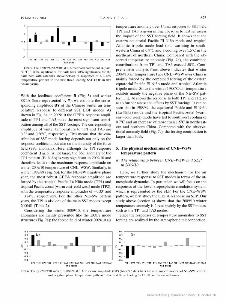
With the feedback coefficient B (Fig. 5) and winter

SSTA (here represented by Y), we estimate the corre-

sponding amplitude BY of the Chinese winter air tem-

perature response to different SST EOF modes. As

shown in Fig. 6a, in 2009/10 the GEFA response ampli-

tude to TP1 and TA3 make the most significant contri-

bution among all of the SST forcings. The corresponding

amplitude of winter temperature to TP1 and TA3 are

0.38 and 0.268C, respectively. This means that the con-

tribution of SST mode forcing depends not only on the

response coefficient, but also on the intensity of the force

field (SST anomaly). Here, although the TP1 response

coefficient (Fig. 5) is not large, the SST anomaly of the

TP1 pattern (El Ni~no) is very significant in 2009/10 and

therefore leads to the maximum response amplitude on

winter 2009/10 temperature of CNE–WSW. Similarly, in

winter 1988/89 (Fig. 6b), for the NE–SW negative phase

year, the most robust GEFA response amplitude are

forced by the tropical Pacific La Ni~na mode (TP1) and

tropical Pacific zonal (warm east–cold west) mode (TP2),

with the temperature response amplitudes of 20.338 and20.248C, respectively. For the other NE–SW pattern

years, the TP1 is also one of the main SST modes except

2000/01 (Table 2).

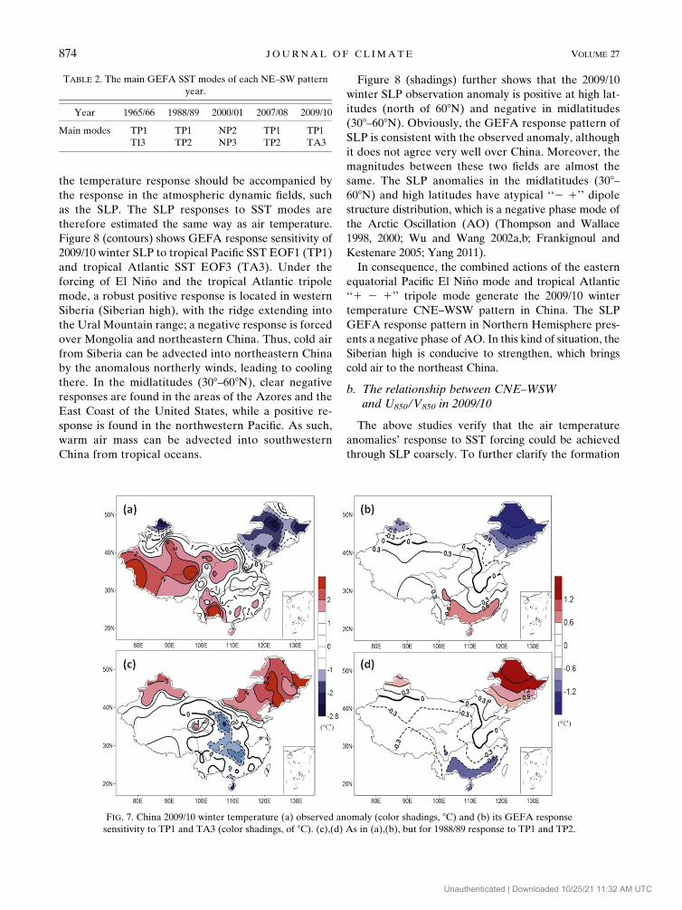
Considering the winter 2009/10, the temperature

anomalies are mainly presented like the EOF2 mode

structure (Fig. 7a); the forced field of winter 2009/10 air

temperature anomaly over China response to SST field

TP1 and TA3 is given in Fig. 7b, so as to further assess

the impact of the SST forcing field. It shows that the

eastern equatorial Pacific El Ni~no mode and tropical

Atlantic tripole mode lead to a warming in south-

western China of 0.98C and a cooling over 1.58C in the

northeast of northern China. Compared with the ob-

served temperature anomaly (Fig. 7a), the combined

contributions from TP1 and TA3 exceed 50%. Com-

prehensive analysis from above indicates that winter

2009/10 air temperature type CNE–WSWover China is

mainly forced by the combined forcing of the eastern

equatorial Pacific El Ni~no mode and tropical Atlantic

tripole mode. Since the winter 1988/89 air temperature

exhibits mainly the negative phase of the NE–SW pat-

tern, Fig. 7d shows the response to both TP1 and TP2, so

as to further assess the effects by SST forcings. It can be

seen that in 1988/89, the equatorial Pacific anti-El Ni~no

(La Ni~na) mode and the tropical Pacific zonal (warm

east–cold west) mode have led to southwest cooling of

0.78C and an increase of more than 1.58C in northeast-

ern and northern China. Compared with the observa-

tional anomaly field (Fig. 7c), the forcing contribution is

larger than 70%.

5. The physical mechanisms of CNE–WSWtemperature pattern

a. The relationship between CNE–WSW and SLPin 2009/10

Here, we further study the mechanism for the air

temperature response to SST modes in terms of the at-

mospheric dynamics. In particular, we will focus on the

responses of the lower-tropospheric circulation system,

which is represented by the SLP. For the CNE–WSW

pattern, we first study the GEFA response on SLP. Our

study above (section 4) shows that the 2009/10 winter

temperature anomaly is forced mainly by the SST modes,

such as the TP1 and TA3 modes.

Since the responses of temperature anomalies to SST

forcing are realized by the atmospheric teleconnection,

FIG. 5. The 1958/59–2009/10GEFA feedback coefficientB (bars,

8C 8C21; 80% significance for dark bars, 90% significance for the

dark bars with asterisks above/below) of responses of NE–SW

temperature pattern to the first three leading SST EOF in five

ocean basins.

FIG. 6. The (a) 2009/10 and (b) 1988/89 GEFA response amplitude (BY) (bars, 8C; dark bars are most import modes) of NE–SW positive

and negative phase temperature pattern to the first three leading SST EOF in five ocean basins.



the temperature response should be accompanied by

the response in the atmospheric dynamic fields, such

as the SLP. The SLP responses to SST modes are

therefore estimated the same way as air temperature.

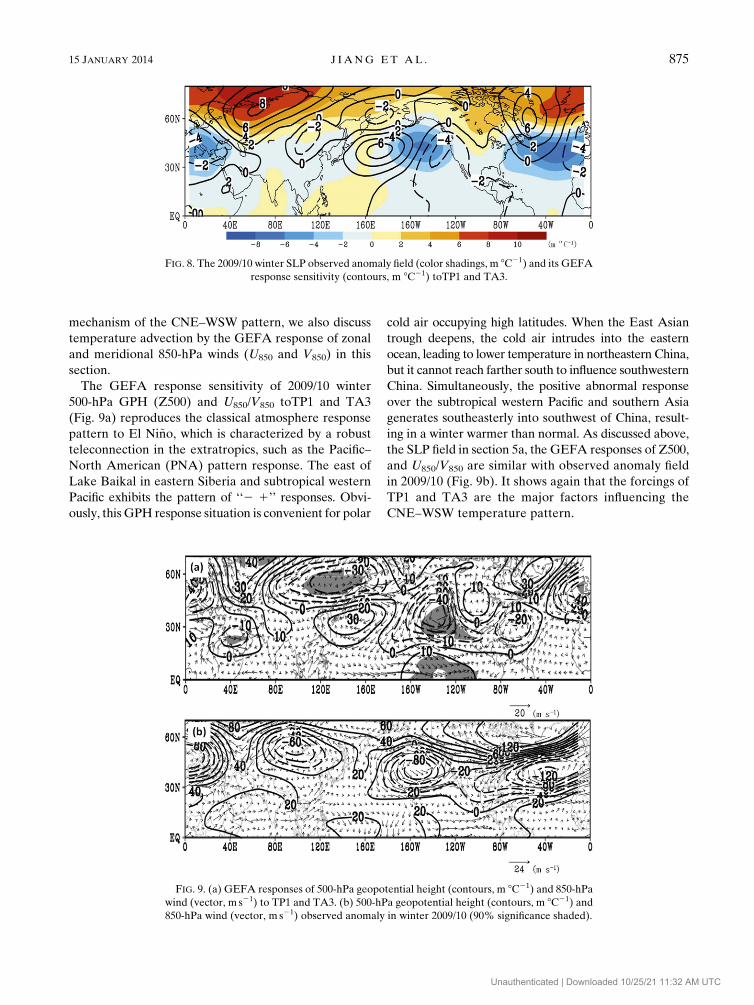
Figure 8 (contours) shows GEFA response sensitivity of

2009/10 winter SLP to tropical Pacific SST EOF1 (TP1)

and tropical Atlantic SST EOF3 (TA3). Under the

forcing of El Ni~no and the tropical Atlantic tripole

mode, a robust positive response is located in western

Siberia (Siberian high), with the ridge extending into

the Ural Mountain range; a negative response is forced

over Mongolia and northeastern China. Thus, cold air

from Siberia can be advected into northeastern China

by the anomalous northerly winds, leading to cooling

there. In the midlatitudes (308–608N), clear negative

responses are found in the areas of the Azores and the

East Coast of the United States, while a positive re-

sponse is found in the northwestern Pacific. As such,

warm air mass can be advected into southwestern

China from tropical oceans.

Figure 8 (shadings) further shows that the 2009/10

winter SLP observation anomaly is positive at high lat-

itudes (north of 608N) and negative in midlatitudes

(308–608N). Obviously, the GEFA response pattern of

SLP is consistent with the observed anomaly, although

it does not agree very well over China. Moreover, the

magnitudes between these two fields are almost the

same. The SLP anomalies in the midlatitudes (308–608N) and high latitudes have atypical ‘‘2 1’’ dipole

structure distribution, which is a negative phase mode of

the Arctic Oscillation (AO) (Thompson and Wallace

1998, 2000; Wu and Wang 2002a,b; Frankignoul and

Kestenare 2005; Yang 2011).

In consequence, the combined actions of the eastern

equatorial Pacific El Ni~no mode and tropical Atlantic

‘‘1 2 1’’ tripole mode generate the 2009/10 winter

temperature CNE–WSW pattern in China. The SLP

GEFA response pattern in Northern Hemisphere pres-

ents a negative phase of AO. In this kind of situation, the

Siberian high is conducive to strengthen, which brings

cold air to the northeast China.

b. The relationship between CNE–WSWand U850 /V850 in 2009/10

The above studies verify that the air temperature

anomalies’ response to SST forcing could be achieved

through SLP coarsely. To further clarify the formation

TABLE 2. The main GEFA SST modes of each NE–SW pattern

year.

Year 1965/66 1988/89 2000/01 2007/08 2009/10

Main modes TP1 TP1 NP2 TP1 TP1

TI3 TP2 NP3 TP2 TA3

FIG. 7. China 2009/10 winter temperature (a) observed anomaly (color shadings, 8C) and (b) its GEFA response

sensitivity to TP1 and TA3 (color shadings, of 8C). (c),(d) As in (a),(b), but for 1988/89 response to TP1 and TP2.



mechanism of the CNE–WSW pattern, we also discuss

temperature advection by the GEFA response of zonal

and meridional 850-hPa winds (U850 and V850) in this

section.

The GEFA response sensitivity of 2009/10 winter

500-hPa GPH (Z500) and U850/V850 toTP1 and TA3

(Fig. 9a) reproduces the classical atmosphere response

pattern to El Ni~no, which is characterized by a robust

teleconnection in the extratropics, such as the Pacific–

North American (PNA) pattern response. The east of

Lake Baikal in eastern Siberia and subtropical western

Pacific exhibits the pattern of ‘‘2 1’’ responses. Obvi-

ously, thisGPH response situation is convenient for polar

cold air occupying high latitudes. When the East Asian

trough deepens, the cold air intrudes into the eastern

ocean, leading to lower temperature in northeastern China,

but it cannot reach farther south to influence southwestern

China. Simultaneously, the positive abnormal response

over the subtropical western Pacific and southern Asia

generates southeasterly into southwest of China, result-

ing in a winter warmer than normal. As discussed above,

the SLP field in section 5a, the GEFA responses of Z500,

and U850/V850 are similar with observed anomaly field

in 2009/10 (Fig. 9b). It shows again that the forcings of

TP1 and TA3 are the major factors influencing the

CNE–WSW temperature pattern.

FIG. 8. The 2009/10 winter SLP observed anomaly field (color shadings, m 8C21) and its GEFA

response sensitivity (contours, m 8C21) toTP1 and TA3.

FIG. 9. (a) GEFA responses of 500-hPa geopotential height (contours, m 8C21) and 850-hPa

wind (vector, m s21) to TP1 and TA3. (b) 500-hPa geopotential height (contours, m 8C21) and

850-hPa wind (vector, m s21) observed anomaly in winter 2009/10 (90% significance shaded).



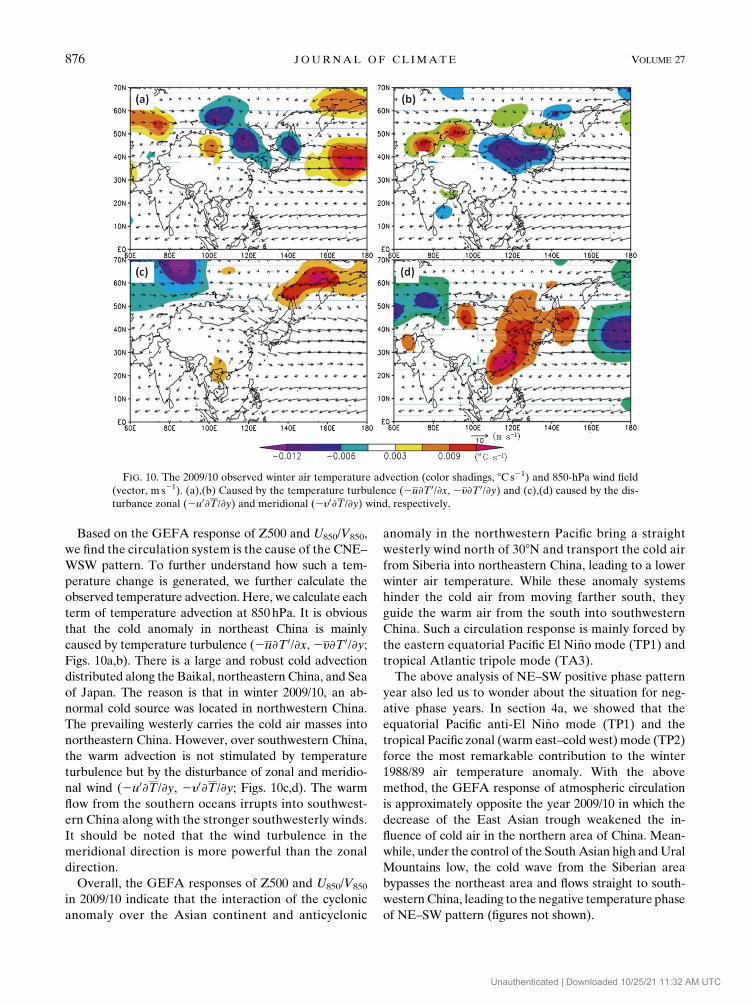
Based on the GEFA response of Z500 and U850/V850,

we find the circulation system is the cause of the CNE–

WSW pattern. To further understand how such a tem-

perature change is generated, we further calculate the

observed temperature advection. Here, we calculate each

term of temperature advection at 850hPa. It is obvious

that the cold anomaly in northeast China is mainly

caused by temperature turbulence (2u›T 0/›x,2y›T 0/›y;Figs. 10a,b). There is a large and robust cold advection

distributed along the Baikal, northeastern China, and Sea

of Japan. The reason is that in winter 2009/10, an ab-

normal cold source was located in northwestern China.

The prevailing westerly carries the cold air masses into

northeastern China. However, over southwestern China,

the warm advection is not stimulated by temperature

turbulence but by the disturbance of zonal and meridio-

nal wind (2u0›T/›y, 2y0›T/›y; Figs. 10c,d). The warm

flow from the southern oceans irrupts into southwest-

ern China along with the stronger southwesterly winds.

It should be noted that the wind turbulence in the

meridional direction is more powerful than the zonal

direction.

Overall, the GEFA responses of Z500 and U850/V850

in 2009/10 indicate that the interaction of the cyclonic

anomaly over the Asian continent and anticyclonic

anomaly in the northwestern Pacific bring a straight

westerly wind north of 308N and transport the cold air

from Siberia into northeastern China, leading to a lower

winter air temperature. While these anomaly systems

hinder the cold air from moving farther south, they

guide the warm air from the south into southwestern

China. Such a circulation response is mainly forced by

the eastern equatorial Pacific El Ni~no mode (TP1) and

tropical Atlantic tripole mode (TA3).

The above analysis of NE–SW positive phase pattern

year also led us to wonder about the situation for neg-

ative phase years. In section 4a, we showed that the

equatorial Pacific anti-El Ni~no mode (TP1) and the

tropical Pacific zonal (warm east–cold west) mode (TP2)

force the most remarkable contribution to the winter

1988/89 air temperature anomaly. With the above

method, the GEFA response of atmospheric circulation

is approximately opposite the year 2009/10 in which the

decrease of the East Asian trough weakened the in-

fluence of cold air in the northern area of China. Mean-

while, under the control of the SouthAsian high andUral

Mountains low, the cold wave from the Siberian area

bypasses the northeast area and flows straight to south-

westernChina, leading to the negative temperature phase

of NE–SW pattern (figures not shown).

FIG. 10. The 2009/10 observed winter air temperature advection (color shadings, 8Cs21) and 850-hPa wind field

(vector, m s21). (a),(b) Caused by the temperature turbulence (2u›T 0/›x, 2y›T 0/›y) and (c),(d) caused by the dis-

turbance zonal (2u0›T/›y) and meridional (2y0›T/›y) wind, respectively.



6. Summary and discussion

To assess the influence of global SST variability on

Chinese winter temperature variability, we examined the

response of the Chinese winter temperature anomaly of

NE–SW pattern to the leading EOF modes of various

oceanic SSTs using the GEFAmethod. While confirming

some previous results, our assessment also unveils some

new features of global oceanic forcing on Chinese winter

temperatures. The main conclusions are as follows.

The second EOF mode (in the period 1958–2010) of

the Chinese winter air temperature anomaly presents a

robust spatial pattern of NE–SW. The main SST forcing

modes for Chinese NE–SWwinter temperature are from

the tropical Pacific and Atlantic. For different years, the

relative importance of the SST modes is different. For

2009/10, the tropical Pacific El Ni~no mode (TP1) and

tropical Atlantic tripole mode (TA3) have the greatest

contribution to the forcing. The GEFA responses of the

atmospheric circulation anomaly suggest that in East

Asia the combinations of TP1 and TA3 generates west-

erly flow and transports cold air from Siberia into

northeastern China, leading to the lower winter tem-

peratures. Meanwhile, in southwestern China the ab-

normal disturbance of meridional wind advects warm

air from the south over the oceans, resulting in warmer

temperature there.

Finally, there aremany further issues to be studied. As

a pilot study here, we only analyzed a few typical years

in detail here. It is not very perfect for some results. In

the future, it will be important to further diagnose and

analyze other years so that wemay find amore systematic

and robust response. The GEFA response of SLP is

largely consistent with the AO pattern. However, the

relationship among SST, AO, and Chinese temperature

remain to be further studied. Finally, in addition to SST

forcing, there may be other factors influencing China

temperature, such as snow coverage and vegetation.

Acknowledgments. We thank Drs. Zhiwei Wu and

Peng Liu for helpful discussions. We also thank the ed-

itor and anonymous reviewers for their constructive

comments. This work is supported jointly by the Na-

tional Basic Research Program 973 (Grant 2010CB950401

and 2012CB955204), Special Research Program for Public

Welfare (Meteorology) of China (GYHY200906016), the

Research and Innovation Project for College Graduates

of Jiangsu Province (782002156), and a Project Funded by

the PriorityAcademic ProgramDevelopment (PAPD) of

Jiangsu Higher Education Institutions.

APPENDIX

The Stability and Sensitivity of Response Estimate B

The three leading modes of these regional EOFs are

combined into a grand set of EOF modes to represent

the ocean forcing in the forcings matrix Tt; we then es-

timate the PC2 of China’s winter temperature (of the

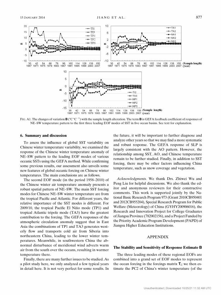
FIG. A1. The changes of variationB (8C 8C21) with the sample length alteration. The termB is GEFA feedback coefficient of responses of

NE–SW temperature pattern to the first three leading EOF modes of SST in five ocean basins. See text for explanation.



NE–SW pattern) to each SST mode in GEFA response

matrix Xt.

Using winters from December 1958 to February 1967

(30 months) as the starting sample length, we examine

the variation of the response value B as a function of

sample sizeN [N5 3i, where i5 10, 11, . . . , 51 (yr)]. As

seen in Fig. A1, all of the values of B tend to be stable

after N exceeds approximately 90. For most leading

modes, the stabilizing sample lengths are even shorter.

For example, the coefficient B stabilizes at about 45

months and 63 months for the first mode of tropical

Pacific Ocean (TP1) and equatorial Indian Ocean mode

(TI1), respectively.

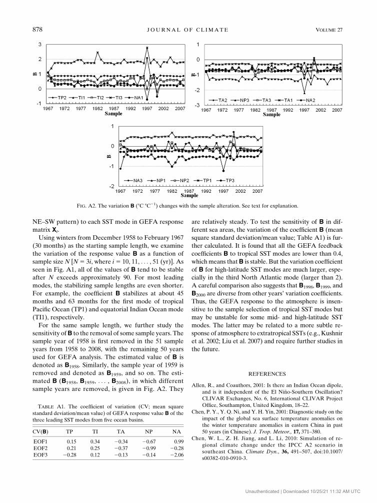
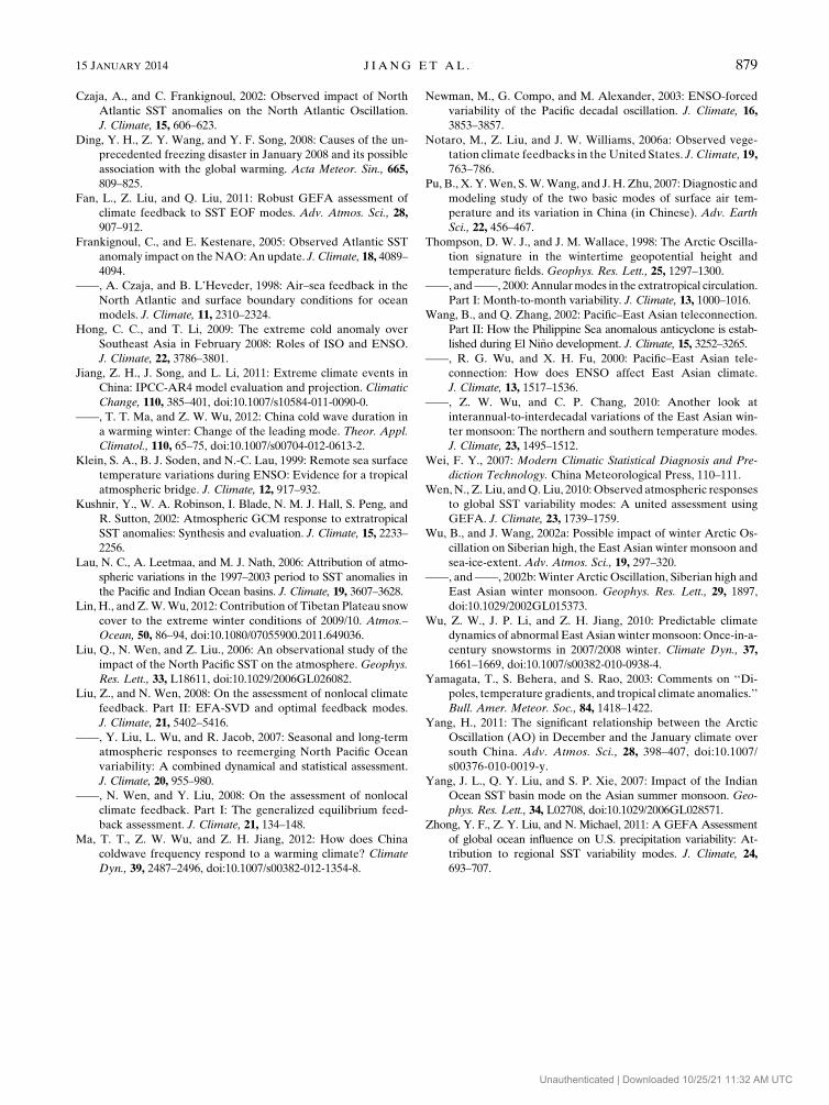
For the same sample length, we further study the

sensitivity ofB to the removal of some sample years. The

sample year of 1958 is first removed in the 51 sample

years from 1958 to 2008, with the remaining 50 years

used for GEFA analysis. The estimated value of B is

denoted as B1958. Similarly, the sample year of 1959 is

removed and denoted as B1959, and so on. The esti-

mated B (B1958, B1959, . . . , B2008), in which different

sample years are removed, is given in Fig. A2. They

are relatively steady. To test the sensitivity of B in dif-

ferent sea areas, the variation of the coefficient B (mean

square standard deviation/mean value; Table A1) is fur-

ther calculated. It is found that all the GEFA feedback

coefficients B to tropical SST modes are lower than 0.4,

whichmeans thatB is stable. But the variation coefficient

of B for high-latitude SST modes are much larger, espe-

cially in the third North Atlantic mode (larger than 2).

A careful comparison also suggests that B1998, B1999, and

B2000 are diverse from other years’ variation coefficients.

Thus, the GEFA response to the atmosphere is insen-

sitive to the sample selection of tropical SST modes but

may be unstable for some mid- and high-latitude SST

modes. The latter may be related to a more subtle re-

sponse of atmosphere to extratropical SSTs (e.g., Kushnir

et al. 2002; Liu et al. 2007) and require further studies in

the future.

REFERENCES

Allen, R., and Coauthors, 2001: Is there an Indian Ocean dipole,

and is it independent of the El Ni~no-Southern Oscillation?

CLIVAR Exchanges, No. 6, International CLIVAR Project

Office, Southampton, United Kingdom, 18–22.

Chen, P. Y., Y. Q. Ni, and Y. H. Yin, 2001: Diagnostic study on the

impact of the global sea surface temperature anomalies on

the winter temperature anomalies in eastern China in past

50 years (in Chinese). J. Trop. Meteor., 17, 371–380.

Chen, W. L., Z. H. Jiang, and L. Li, 2010: Simulation of re-

gional climate change under the IPCC A2 scenario in

southeast China. Climate Dyn., 36, 491–507, doi:10.1007/

s00382-010-0910-3.

FIG. A2. The variation B (8C 8C21) changes with the sample alteration. See text for explanation.

TABLE A1. The coefficient of variation (CV; mean square

standard deviation/mean value) of GEFA response value B of the

three leading SST modes from five ocean basins.

CV(B) TP TI TA NP NA

EOF1 0.15 0.34 20.34 20.67 0.99

EOF2 0.21 0.25 20.37 20.99 20.28

EOF3 20.28 0.12 20.13 20.14 22.06



Czaja, A., and C. Frankignoul, 2002: Observed impact of North

Atlantic SST anomalies on the North Atlantic Oscillation.

J. Climate, 15, 606–623.

Ding, Y. H., Z. Y. Wang, and Y. F. Song, 2008: Causes of the un-

precedented freezing disaster in January 2008 and its possible

association with the global warming. Acta Meteor. Sin., 665,

809–825.

Fan, L., Z. Liu, and Q. Liu, 2011: Robust GEFA assessment of

climate feedback to SST EOF modes. Adv. Atmos. Sci., 28,

907–912.

Frankignoul, C., and E. Kestenare, 2005: Observed Atlantic SST

anomaly impact on the NAO:An update. J. Climate, 18, 4089–4094.

——, A. Czaja, and B. L’Heveder, 1998: Air–sea feedback in the

North Atlantic and surface boundary conditions for ocean

models. J. Climate, 11, 2310–2324.

Hong, C. C., and T. Li, 2009: The extreme cold anomaly over

Southeast Asia in February 2008: Roles of ISO and ENSO.

J. Climate, 22, 3786–3801.Jiang, Z. H., J. Song, and L. Li, 2011: Extreme climate events in

China: IPCC-AR4 model evaluation and projection. Climatic

Change, 110, 385–401, doi:10.1007/s10584-011-0090-0.

——, T. T. Ma, and Z. W. Wu, 2012: China cold wave duration in

a warming winter: Change of the leading mode. Theor. Appl.

Climatol., 110, 65–75, doi:10.1007/s00704-012-0613-2.

Klein, S. A., B. J. Soden, and N.-C. Lau, 1999: Remote sea surface

temperature variations during ENSO: Evidence for a tropical

atmospheric bridge. J. Climate, 12, 917–932.

Kushnir, Y., W. A. Robinson, I. Blade, N. M. J. Hall, S. Peng, and

R. Sutton, 2002: Atmospheric GCM response to extratropical

SST anomalies: Synthesis and evaluation. J. Climate, 15, 2233–

2256.

Lau, N. C., A. Leetmaa, and M. J. Nath, 2006: Attribution of atmo-

spheric variations in the 1997–2003 period to SST anomalies in

the Pacific and Indian Ocean basins. J. Climate, 19, 3607–3628.

Lin, H., and Z.W.Wu, 2012: Contribution of Tibetan Plateau snow

cover to the extreme winter conditions of 2009/10. Atmos.–

Ocean, 50, 86–94, doi:10.1080/07055900.2011.649036.

Liu, Q., N. Wen, and Z. Liu., 2006: An observational study of the

impact of the North Pacific SST on the atmosphere. Geophys.

Res. Lett., 33, L18611, doi:10.1029/2006GL026082.

Liu, Z., and N. Wen, 2008: On the assessment of nonlocal climate

feedback. Part II: EFA-SVD and optimal feedback modes.

J. Climate, 21, 5402–5416.

——, Y. Liu, L. Wu, and R. Jacob, 2007: Seasonal and long-term

atmospheric responses to reemerging North Pacific Ocean

variability: A combined dynamical and statistical assessment.

J. Climate, 20, 955–980.

——, N. Wen, and Y. Liu, 2008: On the assessment of nonlocal

climate feedback. Part I: The generalized equilibrium feed-

back assessment. J. Climate, 21, 134–148.

Ma, T. T., Z. W. Wu, and Z. H. Jiang, 2012: How does China

coldwave frequency respond to a warming climate? Climate

Dyn., 39, 2487–2496, doi:10.1007/s00382-012-1354-8.

Newman, M., G. Compo, and M. Alexander, 2003: ENSO-forced

variability of the Pacific decadal oscillation. J. Climate, 16,

3853–3857.

Notaro, M., Z. Liu, and J. W. Williams, 2006a: Observed vege-

tation climate feedbacks in the United States. J. Climate, 19,

763–786.

Pu, B., X. Y.Wen, S.W.Wang, and J. H. Zhu, 2007: Diagnostic and

modeling study of the two basic modes of surface air tem-

perature and its variation in China (in Chinese). Adv. Earth

Sci., 22, 456–467.

Thompson, D. W. J., and J. M. Wallace, 1998: The Arctic Oscilla-

tion signature in the wintertime geopotential height and

temperature fields. Geophys. Res. Lett., 25, 1297–1300.

——, and——, 2000:Annularmodes in the extratropical circulation.

Part I: Month-to-month variability. J. Climate, 13, 1000–1016.Wang, B., and Q. Zhang, 2002: Pacific–East Asian teleconnection.

Part II: How the Philippine Sea anomalous anticyclone is estab-

lished during El Ni~no development. J. Climate, 15, 3252–3265.

——, R. G. Wu, and X. H. Fu, 2000: Pacific–East Asian tele-

connection: How does ENSO affect East Asian climate.

J. Climate, 13, 1517–1536.

——, Z. W. Wu, and C. P. Chang, 2010: Another look at

interannual-to-interdecadal variations of the East Asian win-

ter monsoon: The northern and southern temperature modes.

J. Climate, 23, 1495–1512.

Wei, F. Y., 2007: Modern Climatic Statistical Diagnosis and Pre-

diction Technology. China Meteorological Press, 110–111.

Wen, N., Z. Liu, andQ. Liu, 2010:Observed atmospheric responses

to global SST variability modes: A united assessment using

GEFA. J. Climate, 23, 1739–1759.Wu, B., and J. Wang, 2002a: Possible impact of winter Arctic Os-

cillation on Siberian high, the East Asian winter monsoon and

sea-ice-extent. Adv. Atmos. Sci., 19, 297–320.

——, and——, 2002b:Winter Arctic Oscillation, Siberian high and

East Asian winter monsoon. Geophys. Res. Lett., 29, 1897,

doi:10.1029/2002GL015373.

Wu, Z. W., J. P. Li, and Z. H. Jiang, 2010: Predictable climate

dynamics of abnormal EastAsianwintermonsoon:Once-in-a-

century snowstorms in 2007/2008 winter. Climate Dyn., 37,

1661–1669, doi:10.1007/s00382-010-0938-4.

Yamagata, T., S. Behera, and S. Rao, 2003: Comments on ‘‘Di-

poles, temperature gradients, and tropical climate anomalies.’’

Bull. Amer. Meteor. Soc., 84, 1418–1422.

Yang, H., 2011: The significant relationship between the Arctic

Oscillation (AO) in December and the January climate over

south China. Adv. Atmos. Sci., 28, 398–407, doi:10.1007/

s00376-010-0019-y.

Yang, J. L., Q. Y. Liu, and S. P. Xie, 2007: Impact of the Indian

Ocean SST basin mode on the Asian summer monsoon. Geo-

phys. Res. Lett., 34, L02708, doi:10.1029/2006GL028571.

Zhong, Y. F., Z. Y. Liu, and N. Michael, 2011: A GEFA Assessment

of global ocean influence on U.S. precipitation variability: At-

tribution to regional SST variability modes. J. Climate, 24,

693–707.



Documents

Assessing the Inﬂuence of Regional SST Modes on the Winter