Spatial Accuracy 2014, East Lansing, Michigan, July 8-11

Assessing the influence of uncertainty in land cover mapping and digital elevation models on flood risk

mapping

LUÍSA M. S. GONÇALVES 1,2,4, CIDÁLIA C FONTE 2,3 RICARDO GOMES1,5

1 Polytechnic Institute of Leiria, School of Technology and Management, Civil Engineering Department, Leiria, Portugal

2 Institute for Systems and Computers Engineering at Coimbra, Coimbra, Portugal 3 Department of Mathematics, University of Coimbra, Coimbra, Portugal 4 ISEGI, Universidade Nova de Lisboa, Lisboa, Portugal 5 IMAR, Universidade de Coimbra, Coimbra, Portugal

Abstract

This paper proposes an approach to assess the influence of the uncertainty present in the parameters dependent on the land cover and elevation data over the peak flow values and the subsequent delineation of flooded areas. The proposed approach was applied to produce vulnerability and risk maps that integrate uncertainty for the urban area of Leiria, Portugal. A SPOT-4 satellite image and DEMs of the region were used. The peak flow was computed using the Soil Conservation Service method and HEC-HMS, HEC-RAS, Matlab and ArcGIS software programs were used. The analysis of the results obtained for the presented case study enables the identification of the order of magnitude of uncertainty associated to the watershed peak flow value and the identification of the areas which are more susceptible to flood risk to be identified.

Keywords: Uncertainty, Watershed Peak flow, Digital Elevation Model, Multispectral Images, Flood Risk Map

1. Introduction

Floods can be defined as an overflow of water from rivers, lakes and weirs. The increase of runoff, in most cases, is caused by intense and concentrated rainfall, but can also have other causes such as thaw, sediment deposition in riverbedsor low capacity of infiltration, among others. The most common floods, and where the economic and social impacts are higher, correspond to an overflow of water from rivers. Presently, as a result of high urban growth, due to the rapid population growth and migration, problems arise due to the use and occupation of the soil (Tucci, 2007). A soil with artificial urban occupation is more impermeable, so the infiltration of runoff is lower, thus increasing the likelihood of downstream flooding. Moreover, changes in topography and/or vegetation as well as clogging and diversion of water lines cause the occurrence of floods and for this reason should be analysed and weighted at the spatial planning level (Jha et al., 2012).

To ensure the safety of people and property, it is necessary to identify flood risk areas and flood control through non-structural solutions (which may work in conjunction with structural solutions) such as forecasting and development of flood warning systems and preparation of emergency plans. In order to implement the most

Spatial Accuracy 2014, East Lansing, Michigan, July 8-11

appropriate flood control proceeding, it is necessary to know the impact of the peak flow for a given return period. However, there is uncertainty associated to the peak flow, as a result of the uncertainty existing in parameters dependent on the type of land cover and the Digital Elevation Model (DEM), which propagate to the results.

There is always uncertainty associated with geographical representation, which comes from the fact that the representations of reality are incomplete and imperfect. The uncertainty existing in the spatial data used for the analysis operations is propagated to the results during the calculation process, influencing the final results. The several sources of uncertainty are then combined, influencing the results in a way that may have negative impacts on the decision making (Ge et al., 2008).

This paper intends to evaluate the effects of several sources of uncertainty that may influence the choice of the hydrological model parameters, such as the Digital Elevation Model (DEM) and the land cover data extracted automatically from multispectral remote sensing images, and to propose a method to model and propagate these sources of uncertainty to the obtained flood risk maps. The proposed methodology was applied to a case study, corresponding to the urban area of Leiria, in Portugal.

2. Data Sets and Methodology

The proposed methodology comprises the following steps:

1) Delineation of the sub-watershed of a river section using different digital elevation models, obtained with different interpolators. The altimetric information was obtained by photogrammetry processes.

2) Production of a Land Cover Map (LCM) using supervised soft classifiers to perform the soft classification of a satellite multispectral image, generating a possibility distribution assigned to each pixel. Since the classification results are influenced by the sample pixels selected as a training set, an automatic method to assist the selection of training samples using ancillary information, the Normalized Difference Vegetation Index and information provided by the classification uncertainty was used, to obtain more accurate outputs. In the presented case study a multispectral SPOT-4 satellite image was used.

3) Calculation of the LCM uncertainty with the application of uncertainty measures. The Relative Maximum Deviation Measure uncertainty measure, available in IDRISI software, was used in the case study.

4) Estimation of the peak flow values for a return period of 100 years, using fuzzy arithmetic and HEC-HMS software. This enables an interval for the peak flow to be generated, which includes all possible peak flow values.

5) Production of the flood risk map and the vulnerability maps according to the land cover in the area under study, using HEC-RAS and ArcGIS software. Flood and risk maps are produced with the representation of uncertainty in the delineation of the flooded area and the flooding risk level.

3. Case Study

3.1. Digital Elevation Model and watershed boundary

Spatial Accuracy 2014, East Lansing, Michigan, July 8-11

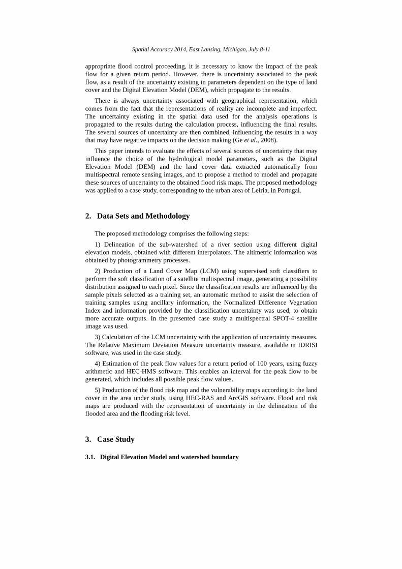
The altimetric information used are elevation contours and elevation points obtained from the digital cartography at the scale 1:10 000 produced using photogrammetry processes. To determine the influence of the DEM in the watershed delineation, 3 DEMs of the study area were produced using: (1) the same interpolation methods spatial resolution (20m) and different spatial altimetric data; (2) different interpolation methods, same resolution (20m) and different spatial altimetric information. The interpolation methods used were Inverse Distance Weigh (IDW) and Discretized Thin Plate Spline (DTPS); both methods are available in ArcGIS software. The DEMs produced were used to delineate the watershed areas. The differences between the watersheds obtained with the different DEMs were analysed using GIS technology. A watershed that only includes the pixels belonging to all obtained watershed versions was also identified, which corresponds to the regions that, according to the approaches used, belong to the watershed. Figure 1 shows the several DEM obtained with the different interpolation methods and different spatial data. Figure 2 shows the watershed boundary using different DEMs.

Figure 1: DEM obtained with the different interpolation methods and different spatial data.

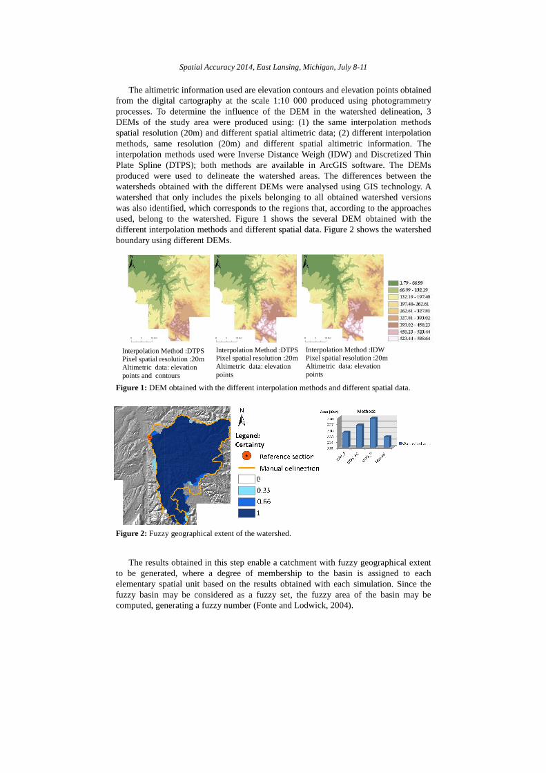
Figure 2: Fuzzy geographical extent of the watershed.

The results obtained in this step enable a catchment with fuzzy geographical extent to be generated, where a degree of membership to the basin is assigned to each elementary spatial unit based on the results obtained with each simulation. Since the fuzzy basin may be considered as a fuzzy set, the fuzzy area of the basin may be computed, generating a fuzzy number (Fonte and Lodwick, 2004).

Interpolation Method :DTPS Pixel spatial resolution :20m Altimetric data: elevation points and contours

Interpolation Method :DTPS Pixel spatial resolution :20m Altimetric data: elevation points

Interpolation Method :IDW Pixel spatial resolution :20m Altimetric data: elevation points

Spatial Accuracy 2014, East Lansing, Michigan, July 8-11

3.2. Production of Land Cover Map and Land Cover Map uncertainty

SPOT-4 multispectral images of the Leiria region of 2006 were used to generate the LCM. The images have a spatial resolution of 20m and 4 spectral bands, green (0.50-0.59 µm), red (0.61-0.68 µm), near infrared (0.78-0.89 µm) and short-wavelength infrared (1.58-1.75 µm) (see Figure 3).

Figure 3: Left: SPOT-4 image (321) of the study area; Right: location of the sub-watershed in Leiria Municipality.

The classification method used is based on the maximum likelihood classifier (Bayes classifier). The traditional use of this classification method assigns each pixel to the class corresponding to the highest probability density function value. However, the posterior probabilities can be computed from the probability density functions (Foody et al., 1992). These posterior probabilities add up to one for each pixel, and may be interpreted as representing the proportional cover of the classes in each pixel or as indicators of the uncertainty associated with the pixel allocation to the classes (Ibrahim et al., 2005). In this paper, this second interpretation is followed.

The methodology used consisted of the following steps: (1) establishment of the protocol and selection of the training and testing sample pixels; (2) performing a soft classification with the defined training sample; (3) extracting the degree of uncertainty of the classification for the pixels in the training sample; (4) eliminating the training sample pixels with low levels of certainty; (5) classification of the image with the modified training sample; and (6) evaluating the classification accuracy. The classes used in this classification were: Artificial Areas (AA); Barren Areas (BA), Irrigated Herbaceous Crops (IHC); Forest Areas (FA), Heterogeneous Agriculture Areas (HA) and Shrub Lands (SL). The uncertainty was evaluated for each pixel using the uncertainty measure E, developed by Chow (1970), and given by Equation (1):

( ) ( )E 1x p x= − (1)

where ( )p x is the largest degree of probability of the probability distributions assigned

to pixel x.

The accuracy assessment was made with an error matrix and the Overall Accuracy was computed as well the User and Producer Accuracy indices for all classes. The total sample size used for testing included 600 pixels, selected using a stratified random sampling of 100 pixels per class. The information of reference data for these pixels was obtained from aerial images with finer spatial resolution.

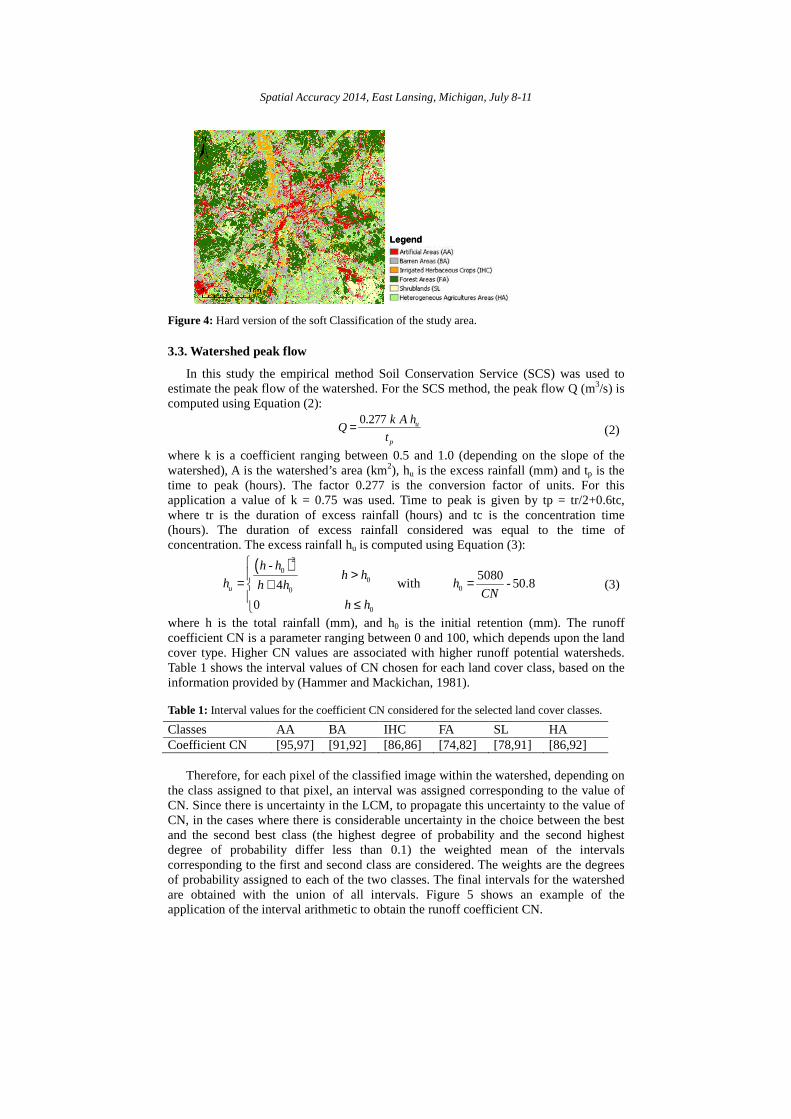
The Global Accuracy of the classification with SPOT-4 satellite images was 72%. Figure 4 shows the hard version of the classification results (the best class assigned to each pixel).

Reference section (Arrabalde, Leiria)

Spatial Accuracy 2014, East Lansing, Michigan, July 8-11

Figure 4: Hard version of the soft Classification of the study area.

3.3. Watershed peak flow

In this study the empirical method Soil Conservation Service (SCS) was used to estimate the peak flow of the watershed. For the SCS method, the peak flow Q (m3/s) is computed using Equation (2):

0.277 = u

p

k A hQ

t (2)

where k is a coefficient ranging between 0.5 and 1.0 (depending on the slope of the watershed), A is the watershed’s area (km2), hu is the excess rainfall (mm) and tp is the time to peak (hours). The factor 0.277 is the conversion factor of units. For this application a value of k = 0.75 was used. Time to peak is given by tp = tr/2+0.6tc, where tr is the duration of excess rainfall (hours) and tc is the concentration time (hours). The duration of excess rainfall considered was equal to the time of concentration. The excess rainfall hu is computed using Equation (3):

( )2

00

00

0

- 5080

with - 50.84

0

>= =+

≤

u

h hh h

h hh hCN

h h

(3)

where h is the total rainfall (mm), and h0 is the initial retention (mm). The runoff coefficient CN is a parameter ranging between 0 and 100, which depends upon the land cover type. Higher CN values are associated with higher runoff potential watersheds. Table 1 shows the interval values of CN chosen for each land cover class, based on the information provided by (Hammer and Mackichan, 1981). Table 1: Interval values for the coefficient CN considered for the selected land cover classes.

Classes AA BA IHC FA SL HA Coefficient CN [95,97] [91,92] [86,86] [74,82] [78,91] [86,92] Therefore, for each pixel of the classified image within the watershed, depending on the class assigned to that pixel, an interval was assigned corresponding to the value of CN. Since there is uncertainty in the LCM, to propagate this uncertainty to the value of CN, in the cases where there is considerable uncertainty in the choice between the best and the second best class (the highest degree of probability and the second highest degree of probability differ less than 0.1) the weighted mean of the intervals corresponding to the first and second class are considered. The weights are the degrees of probability assigned to each of the two classes. The final intervals for the watershed are obtained with the union of all intervals. Figure 5 shows an example of the application of the interval arithmetic to obtain the runoff coefficient CN.

LegendLegend

Spatial Accuracy 2014, East Lansing, Michigan, July 8-11

Figure 5: Example of the application of interval arithmetic to obtain the runoff coefficient CN. The catchment peak flow is then evaluated for the basin using fuzzy arithmetic. With this methodology a fuzzy number is obtained for the peak flow, which indicates all possible peak flow values and the possibility of their occurrence.

3.4. Production of the flood risk map and the vulnerability maps

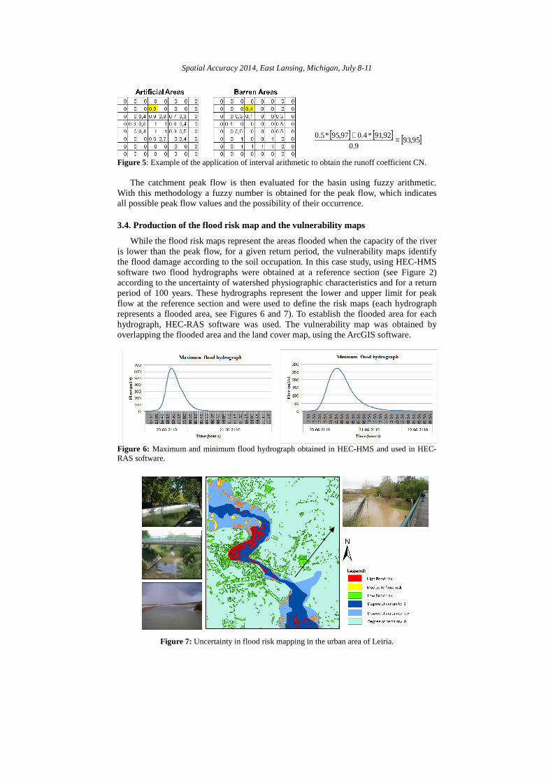
While the flood risk maps represent the areas flooded when the capacity of the river is lower than the peak flow, for a given return period, the vulnerability maps identify the flood damage according to the soil occupation. In this case study, using HEC-HMS software two flood hydrographs were obtained at a reference section (see Figure 2) according to the uncertainty of watershed physiographic characteristics and for a return period of 100 years. These hydrographs represent the lower and upper limit for peak flow at the reference section and were used to define the risk maps (each hydrograph represents a flooded area, see Figures 6 and 7). To establish the flooded area for each hydrograph, HEC-RAS software was used. The vulnerability map was obtained by overlapping the flooded area and the land cover map, using the ArcGIS software. Figure 6: Maximum and minimum flood hydrograph obtained in HEC-HMS and used in HEC-RAS software.

Figure 7: Uncertainty in flood risk mapping in the urban area of Leiria.

[ ] [ ] [ ]95,939.0

92,91*4.097,95*5.0 =+

Spatial Accuracy 2014, East Lansing, Michigan, July 8-11

4. Conclusion

The results show that the influence of uncertainty may have a significant effect on the delineation of flood risk maps in urban areas. For example, the differences in the area obtained for the watersheds generated using DEMs with different methods is, in some cases, almost 20%, showing that the watershed delineation method may influence the results considerably, especially in the flatter areas. By using this method, instead of obtaining one peak flood value, an interval is obtained for the peak flood which allows different levels of flood risk mapping in urban areas to be defined, according to the degree of uncertainty. This methodology can be useful to define the levels of risk used by insurance companies.

Acknowledgments

Luisa M. S. Gonçalves and Cidália C. Fonte work was partially supported by the Portuguese Foundation for Science and Technology under project grant PEst-OE/ EEI/UI308/2014

References

Chow, C.K. (1970), “On optimum error and reject tradeoff”. IEEE Transactions on Information Theory. Vol. 16: 41–46.

Fonte, C. C., Lodwick, W. A. (2004), "Areas of fuzzy geographical entities", International Journal of Geographical Information Science, Vol. 18(2): 127 - 150.

Foody, G. M., Campbell, N.A., Trodd, N.M. and Wood, T.F. (1992), “Derivation and applications of probabilistic measures of class membership from maximum likelihood classification”. Photogrammetric Engineering and Remote Sensing, Vol. 58: 1335-1341.

Ge, Y., Li, S., Duan, R., Bai, H., Cao, F. (2008) "Multi-level Measurements for Uncertainty in Classified Remotely Sensed Imagery". Proceedings of the 8th International Symposium on Spatial Accuracy Assessment in Natural Resources and Environmental Sciences, Shanghai, China, pp. 171-178.

Hammer, J., Mackichan, A. (1981) Hydrology and Quality of Water Resources. John Wiley & Sons, New York, New York, USA.

Ibrahim, M. A., Arora, M. K. and Ghosh, S. K. (2005), “Estimating and accommodating uncertainty through the soft classification of remote sensing data”. International Journal of Remote Sensing, Vol. 26: 2995-3007.

Jha, A. K, Bloch, R., Lamond, J. (2012), Cidades e Inundações (Um guia para a Gestão Integrada do Risco de Inundação Urbana para o Século XXI), The World Bank, Washington, D.C., 54p.

Liu, Y. B., Smedt, F. (2005), "Flood Modeling for Complex Terrain Using GIS and Remote Sensed Information". Water Resources Management, Vol. 19: 605-624.

Tucci, C. E. M (2007), Urban Flood Management. World Meteorological Organization, Geneva, Switzerland, 303p.