Assessing the impacts of agricultural policy and structural reforms

on income distribution and poverty in Brazil •

Carlos R. Azzoni, Tatiane A. Menezes,

Fernando G. Silveira, Eduardo A. Haddad

Joaquim M. Guilhoto, and Heron C. E. Carmo

University of São Paulo and Fipe, Brazil

1. Introduction

Producers and households in developing countries are affected by the prices of

products involved in international transactions. The impacts of agricultural policy and

structural reforms leading to changes in international prices of goods and services are

expected to be differentiated across households and producers, depending on how they are

involved in the circular flow of goods and services within the country of residence. As

such, it might be expected that these reforms will affect income distribution and poverty

levels within those countries.

• This is a progress report of a study developed under the 'Distributional Effects of Agriculture and Trade Policy on Developed and Developing Countries' project of OECD. It was prepared for presentation at the Global Forum on Agriculture, OECD, Paris, December 10-11, 2003.

Considering the supply side, units producing commodities facing price increases in

the international markets will benefit, since their product will become more valuable; those

using imported inputs whose prices increased as a result of the structural reforms will lose.

As for households, those working in sectors with increased international prices could

experience income gains, and those working in other sectors could rest unaffected in terms

of income. However, since some prices would rise, households not working for gaining

sectors could suffer a decrease in real income. A general price increase could also result,

thus affecting all sorts of households.

Therefore, structural reforms that can change international prices are expected to

produce important changes in income distribution in all countries involved in international

trade. Since the impacts will vary according to the role played by different agents in the

production and distribution of national income, it is important to produce a detailed

analysis of such impacts.

The objective of this study is to produce an estimate of the impacts of agricultural

policy and structural reforms on income distribution and poverty in Brazil, considering not

only the first round (direct) effects but also their spillovers (indirect effects) across the

circular flow of income. The introduction of the second and higher round effects is

important, for the initial effects could either be mitigated or empowered by the indirect

effects.

The knowledge of such compounded effects is important in the design of alternative

policies for cushioning the measured adverse impacts of reforms on poor people. It is

possible that an increase in the price of a very important export product of a country does

not necessarily benefit all households equally. As a matter of fact, some may be badly hurt,

if the prices of products with high participation in their consumption basket increased as a

result of the second and higher order effects in the national economy, and if they do not

work in sectors benefited by the initial price increase.

The relationship between income and consumption in the economic system is such

that: a) consumption level depends on the structure of income distribution; b) consumption

structure is different across income groups; and c) consumption structure determines

employment, income level, and income distribution in the economy. These links can be

studied through a Social Accounting Matrix model. We plan to construct such a model for

Brazil, as will be presented later on in this report, and use it to estimate the impacts of

changes in international prices of agricultural products on income distribution and poverty

in Brazil.

2. Methodology and data sources

2.1. The SAM framework

When constructing a SAM, besides the need to fulfill its theoretical requirements,

one must pay attention to the use that the SAM its going to be put to, i.e., the goals of the

study should direct its final structure. With the above in mind, the SAM for the Brazilian

model must make a distinction between the agricultural and nonagricultural activities and

agents in the economy, and take into consideration the relations that occur between them.

At the same time, the SAM should also take into consideration the relation with agricultural

and nonagricultural activities and agents with the rest of the world economy.

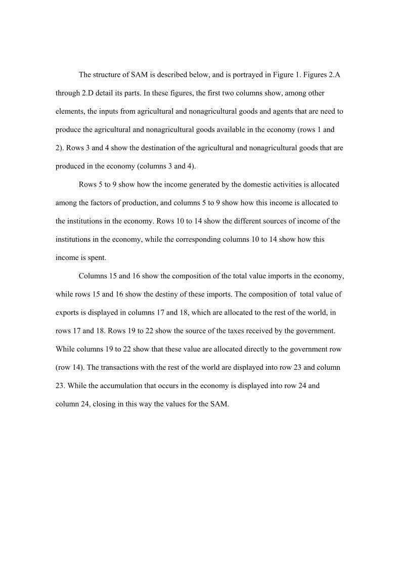
The structure of SAM is described below, and is portrayed in Figure 1. Figures 2.A

through 2.D detail its parts. In these figures, the first two columns show, among other

elements, the inputs from agricultural and nonagricultural goods and agents that are need to

produce the agricultural and nonagricultural goods available in the economy (rows 1 and

2). Rows 3 and 4 show the destination of the agricultural and nonagricultural goods that are

produced in the economy (columns 3 and 4).

Rows 5 to 9 show how the income generated by the domestic activities is allocated

among the factors of production, and columns 5 to 9 show how this income is allocated to

the institutions in the economy. Rows 10 to 14 show the different sources of income of the

institutions in the economy, while the corresponding columns 10 to 14 show how this

income is spent.

Columns 15 and 16 show the composition of the total value imports in the economy,

while rows 15 and 16 show the destiny of these imports. The composition of total value of

exports is displayed in columns 17 and 18, which are allocated to the rest of the world, in

rows 17 and 18. Rows 19 to 22 show the source of the taxes received by the government.

While columns 19 to 22 show that these value are allocated directly to the government row

(row 14). The transactions with the rest of the world are displayed into row 23 and column

23. While the accumulation that occurs in the economy is displayed into row 24 and

column 24, closing in this way the values for the SAM.

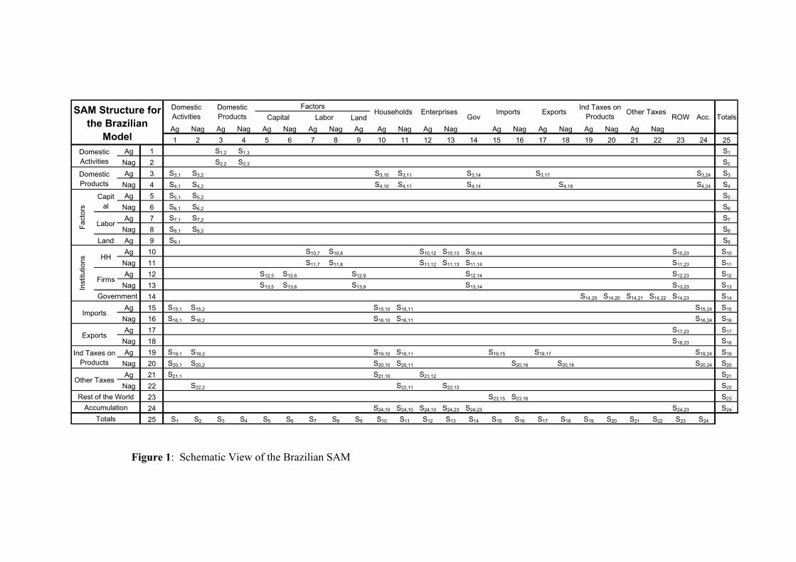
Figure 1: Schematic View of the Brazilian SAM

LandAg Nag Ag Nag Ag Nag Ag Nag Ag Ag Nag Ag Nag Ag Nag Ag Nag Ag Nag Ag Nag1 2 3 4 5 6 7 8 9 10 11 12 13 14 15 16 17 18 19 20 21 22 23 24 25

Ag 1 S1,2 S1,3 S1

Nag 2 S2,2 S2,3 S2

Ag 3 S3,1 S3,2 S3,10 S3,11 S3,14 S3,17 S3,24 S3

Nag 4 S4,1 S4,2 S4,10 S4,11 S4,14 S4,18 S4,24 S4

Ag 5 S5,1 S5,2 S5

Nag 6 S6,1 S6,2 S6

Ag 7 S7,1 S7,2 S7

Nag 8 S8,1 S8,2 S8

Land Ag 9 S9,1 S9

Ag 10 S10,7 S10,8 S10,12 S10,13 S10,14 S10,23 S10

Nag 11 S11,7 S11,8 S11,12 S11,13 S11,14 S11,23 S11

Ag 12 S12,5 S12,6 S12,9 S12,14 S12,23 S12

Nag 13 S13,5 S13,6 S13,9 S13,14 S13,23 S13

14 S14,20 S14,20 S14,21 S14,22 S14,23 S14

Ag 15 S15,1 S15,2 S15,10 S15,11 S15,24 S15

Nag 16 S16,1 S16,2 S16,10 S16,11 S16,24 S16

Ag 17 S17,23 S17

Nag 18 S18,23 S18

Ag 19 S19,1 S19,2 S19,10 S19,11 S19,15 S19,17 S19,24 S19

Nag 20 S20,1 S20,2 S20,10 S20,11 S20,16 S20,18 S20,24 S20

Ag 21 S21,1 S21,10 S21,12 S21

Nag 22 S22,2 S22,11 S22,13 S22

23 S23,15 S23,16 S23

24 S24,10 S24,10 S24,10 S24,23 S24,23 S24,23 S24

25 S1 S2 S3 S4 S5 S6 S7 S8 S9 S10 S11 S12 S13 S14 S15 S16 S17 S18 S19 S20 S21 S22 S23 S24

Rest of the WorldAccumulation

Totals

Imports

Exports

Ind Taxes on Products

Other Taxes

Inst

itutio

ns HH

Firms

Government

Domestic Activities

Domestic Products

Fact

ors

Capital

Labor

Acc. TotalsCapital LaborExports Ind Taxes on

Products Other TaxesROW

Households EnterprisesGov

ImportsSAM Structure for the Brazilian

Model

Domestic Activities

Domestic Products

Factors

Figure 2A – Structure of Brazilian SAM – Part 1 of 4

Agriculture Nonagriculture Agriculture Nonagriculture

1 2 3 4

Agriculture 1 Domestic sales agric goods

Domestic sales nonagric goods

Nonagriculture 2 Domestic sales agric goods

Domestic sales nonagric goods

Agriculture 3 Int. demand for agric. goods

Int. demand for agric. goods

Nonagriculture 4 Int. demand for nonagric. goods

Int. demand for nonagric. goods

Agriculture 5 Capital Income from agriculture

Capital Income from nonagric.

Nonagriculture 6 Capital Income from agriculture

Capital Income from nonagric.

Agriculture 7 Labor Income from agriculture

Labor Income from nonagric.

Nonagriculture 8 Labor Income from agriculture

Labor Income from nonagric.

Land Agriculture 9 Land Income from

agriculture

Agriculture 10

Nonagriculture 11

Agriculture 12

Nonagriculture 13

14

Agriculture 15Imports of agric

goods for production

Imports of agric goods for production

Nonagriculture 16Imports of

nonagric goods for procduction

Imports of nonagric goods for

procduction

Agriculture 17

Nonagriculture 18

Agriculture 19 Indirect taxes on agriculture inputs

Indirect taxes on agriculture inputs

Nonagriculture 20Indirect taxes on nonagriculture

inputs

Indirect taxes on nonagriculture

inputs

Imports

Exports

Indirect Taxes on Products

Inst

itutio

ns

Hou

seho

lds

Ente

rpris

es

Government

Domestic Activities

Domestic Products

Fact

ors

Cap

ital

Labo

r

SAM Structure for the Brazilian Model - 1999

Domestic Activities Domestic Products

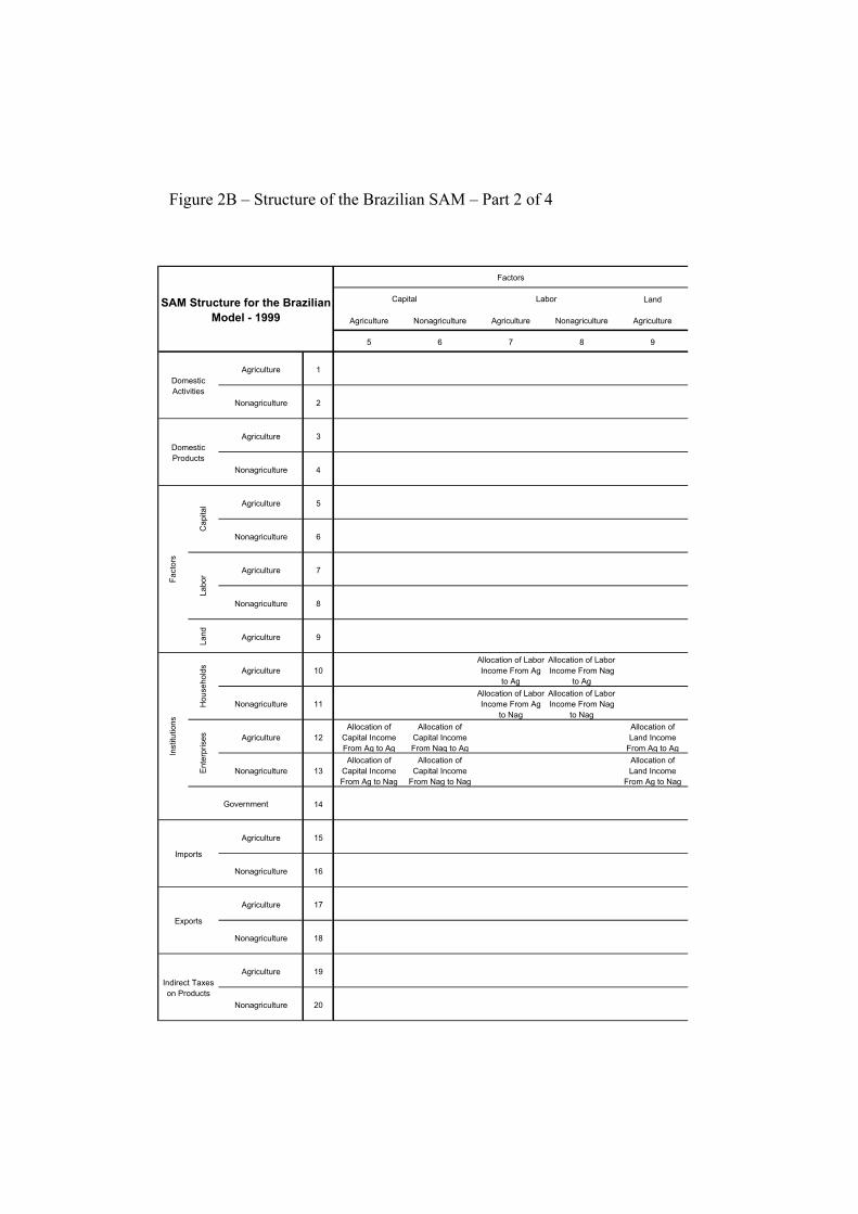
Figure 2B – Structure of the Brazilian SAM – Part 2 of 4

Land

Agriculture Nonagriculture Agriculture Nonagriculture Agriculture

5 6 7 8 9

Agriculture 1

Nonagriculture 2

Agriculture 3

Nonagriculture 4

Agriculture 5

Nonagriculture 6

Agriculture 7

Nonagriculture 8

Land Agriculture 9

Agriculture 10Allocation of Labor Income From Ag

to Ag

Allocation of Labor Income From Nag

to Ag

Nonagriculture 11Allocation of Labor Income From Ag

to Nag

Allocation of Labor Income From Nag

to Nag

Agriculture 12Allocation of

Capital Income From Ag to Ag

Allocation of Capital Income From Nag to Ag

Allocation of Land Income

From Ag to Ag

Nonagriculture 13Allocation of

Capital Income From Ag to Nag

Allocation of Capital Income

From Nag to Nag

Allocation of Land Income

From Ag to Nag

14

Agriculture 15

Nonagriculture 16

Agriculture 17

Nonagriculture 18

Agriculture 19

Nonagriculture 20

Imports

Exports

Indirect Taxes on Products

Inst

itutio

ns

Hou

seho

lds

Ente

rpris

es

Government

Domestic Activities

Domestic Products

Fact

ors

Cap

ital

Labo

r

Capital LaborSAM Structure for the Brazilian Model - 1999

Factors

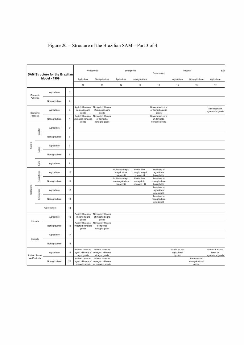
Figure 2C – Structure of the Brazilian SAM – Part 3 of 4

Agriculture Nonagriculture Agriculture Nonagriculture Agriculture Nonagriculture Agriculture

10 11 12 13 14 15 16 17

Agriculture 1

Nonagriculture 2

Agriculture 3Agric HH cons of domestic agric

goods

Nonagric HH cons of domestic agric

goods

Government cons of domestic agric

goods

Net exports of agricultural goods

Nonagriculture 4Agric HH cons of

domestic nonagric goods

Nonagric HH cons of domestic

nonagric goods

Government cons of domestic

nonagric goods

Agriculture 5

Nonagriculture 6

Agriculture 7

Nonagriculture 8

Land Agriculture 9

Agriculture 10Profits from agric

to agriculture household

Profits from nonagric to agric

household

Transfers to agriculture households

Nonagriculture 11Profits from agric to nonagriculture

household

Profits from nonagric to

nonagric HH

Transfers to nonagriculture

households

Agriculture 12Transfers to agriculture enterprises

Nonagriculture 13Transfers to

nonagriculture enterprises

14

Agriculture 15Agric HH cons of

imported agric goods

Nonagric HH cons of imported agric

goods

Nonagriculture 16Agric HH cons of imported nonagric

goods

Nonagric HH cons of imported

nonagric goods

Agriculture 17

Nonagriculture 18

Agriculture 19Indirect taxes on agric HH cons of

agric goods

Indirect taxes on nonagric HH cons

of agric goods

Tariffs on imp agricultural

goods

Indirect & Export taxes on

agricultural goods

Nonagriculture 20Indirect taxes on agric HH cons of nonagric goods

Indirect taxes on nonagric HH cons of nonagric goods

Tariffs on imp nonagricultural

goods

Imports

Exports

Indirect Taxes on Products

Inst

itutio

ns

Hou

seho

lds

Ente

rpris

es

Government

Domestic Activities

Domestic Products

Fact

ors

Cap

ital

Labo

r

ExpHouseholds EnterprisesGovernment

Imports

SAM Structure for the Brazilian Model - 1999

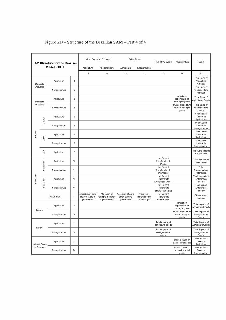
Figure 2D – Structure of the Brazilian SAM – Part 4 of 4

Agriculture Nonagriculture Agriculture Nonagriculture

19 20 21 22 23 24 25

Agriculture 1Total Sales of

Agricultural Activities

Nonagriculture 2Total Sales of

Nonagricultural Activities

Agriculture 3Investment

expenditure on dom agric goods

Total Sales of Agricultural Goods

Nonagriculture 4Invest expenditure on dom nonagric

goods

Total Sales of Nonagricultural

Goods

Agriculture 5Total Capital

Income in Agriculture

Nonagriculture 6Total Capital

Income in Nonagriculture

Agriculture 7Total Labor Income in Agriculture

Nonagriculture 8Total Labor Income in

Nonagriculture

Land Agriculture 9 Total Land Income

in Agriculture

Agriculture 10Net Current

Transfers to HH (Agric)

Total Agriculture HH Income

Nonagriculture 11Net Current

Transfers to HH (Nonagric)

Total Nonagriculture

HH Income

Agriculture 12Net Current Transfers to

Enterprises (Agric)

Total Agriculture Enterprises

Income

Nonagriculture 13Net Current Transfers to

Enterp (Nonagric)

Total Nonag Enterprises

Income

14Allocation of agric indirect taxes to

government

Allocation of nonagric ind taxes

to government

Allocation of agric other taxes to government

Allocation of nonagric other taxes to gov

Net Current Transfers to Government

Government Income

Agriculture 15Investment

expenditure on imp agric goods

Total Imports of Agriculture Goods

Nonagriculture 16Invest expenditure on imp nonagric

goods

Total Imports of Nonagriculture

Goods

Agriculture 17 Total exports of agricultural goods

Total Exports of Agriculture Goods

Nonagriculture 18Total exports of nonagricultural

goods

Total Exports of Nonagriculture

Goods

Agriculture 19 Indirect taxes on agric capital goods

Total Indirect Taxes on

Agriculture

Nonagriculture 20Indirect taxes on nonagric capital

goods

Total Indirect Taxes on

Nonagriculture

Imports

Exports

Indirect Taxes on Products

Inst

itutio

ns

Hou

seho

lds

Ente

rpris

es

Government

Domestic Activities

Domestic Products

Fact

ors

Cap

ital

Labo

r

Accumulation TotalsIndirect Taxes on Products Other Taxes

Rest of the WorldSAM Structure for the Brazilian Model - 1999

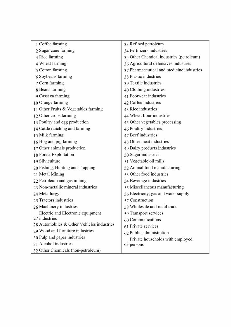
2.2. Sectoral disaggregation

Previous applications of this model for the Brazilian economy can be found in

Fonseca and Guilhoto (1987), and Guilhoto, Conceição, and Crocomo (1996). The input-

output matrices released by the Brazilian Statistical Institute (IBGE) only take into

consideration the Agriculture as a whole and 7 food processing industries, of a total of 42

sectors. The most recent data released from IBGE refers to the year of 1996; this matrix

was up-dated to the year 1999, following the methodology developed by Guilhoto et al

(2002), based on Brazilian national accounts. Given data constraints, the maximum

possible disaggregation is disposed in table 1 below. Agriculture was broken down into 17

sectors, and food-processing industries were disaggregated into 12 sectors, including

alcohol, that is treated separately from the chemical sector. The other sectors are the same

as in the official national input-output matrix.

Table 2 presents the importance of 33 sectors representing agribusiness activities in

Brazil. The first column indicates the importance of each sector in total national

production; the second presents the shares within the 33-sector group. It can be seen that

this group of sectors accounts for only 15.3% of total national production, in spite of the

fact that Brazil is a major world producer of several products. This reflects the fact that

Brazil presents a large and diversified economy. The next two columns indicate the

destination of production to domestic household consumption and to exports. These two

destinations are important in terms of internal income distribution and in terms of

competitiveness of the country. Export-oriented sectors, such as coffee, sugar, and soybean,

compete in the international market and are prone to be the first affected by different

conditions in the world food market. On the other hand, sectors oriented towards the local

market, such as rice, beans, manioc, beef, dairy, etc., will lead important internal

distributional impacts in case of changes in world prices.

3. Household and farmer typology

The definition of farm types is based on two different data sets: the Agricultural

Census of 1996/97 and the Pesquisa Padrão de Vida (PPV) of 1996, both from IBGE. The

first source is more comprehensive and allows for more information across states, farm

sizes, technology, etc. The second source provides more information on household

characteristics, consumption structures, etc.

Starting with the census, our definition of household types is be based on the study

by the Ministry of Agrarian Reform/Incra and FAO. In that study, Brazilian farms were

split into family and non-family, based on size, use of hired labor, etc. Family farms were

split into 4 groups, based on value added; non-family farms were split into 3 groups, based

on technology and size. Based on the objectives of this study, and on our analysis of

characteristics of family and non-family farms, we have decided to work with four groups

of family farms, and to deal with non-family farms as a sole group.

Since we will use information from two different sources, it is important to analyze

the matching of those two in terms of general characteristics of farmers. Therefore, we have

allocated PPV farmers into the five groups defined above. Results are displayed in Table 3.

Comparing the proportions of area, number of farms and number of people working

in the different farm types, it can be seen that the distributions in the two data sets are quite

similar. In other words, PPV consists of a good sample for the census results. This

conclusion is even stronger if we consider that some variables have different definitions in

the two data sets. For example, the census study considers total farm size, while PPV

considers only cultivated area. This explains why the sizes in the latter are smaller for all

farm types. The same holds for income variables: census deals with value added while PPV

considers income. Given these different definitions, proportions of income by farmer type

across data sets are not as similar as for the other variables. For comparison purposes only,

we have excluded from PPV household heads with non-farm incomes (heads living in the

rural area but working in urban activities) and have imposed a limit to property size,

arriving at the income per farm figures of table 3.

The second part of table 3 presents some indicators of input use. Since our

definition of “other” types of energy is more restrictive than the census classification, we

came up with higher proportions of manual use of energy and smaller proportions of animal

and “other”. However, comparing the distribution of proportions according to household

types, it can be seen that in general the same pattern holds for both classifications. The last

three columns present the value and distribution of expenditures by household type in PPV,

indicating a clear differentiation between family and non-family farms.

As a result of these comparisons, we are quite confident that we can use PPV

information to supplement census data whenever necessary in the study. This will be

particularly important when we consider the consumption structure of household types.

Urban households were split into four groups, based on income level. A group comprising

only agricultural employees is also included.

Table 4 presents the sources of monetary income for the ten groups of households

defined above. It can be seen that wages account for 23% of monetary income for family

farmers 1, and around 31% for family farmers 2 and 3. For the fourth type of family

farmers, it goes up to 56%. For agricultural employees it is even higher, 70%. Income from

self-employment is low for family farmers in general, being higher for family farmers 3. As

expected, it is highest for business farmers (type 5). For urban households, the importance

of wage income does not vary much, being 40% for the poorest, and around 47%-48% for

the other three groups.

4. Distributional aspects

It was pointed out before that different sectors present different linkages within the

production system, be it through technical relationships with other sectors, or through

income generation and distribution, and, hence, through consumption, as a feed-back

mechanism. Therefore, it is important to take into consideration how wages and value

added are distributed to different groups of income. Figures 1 and 2, showing the

distribution of wages and value added to income deciles, present an example of how sectors

are heterogeneous in this respect. Figure 1 indicates that, from all wage income received by

the lowest income group, farm sectors are responsible for 20%, increasing to 24% in the

next decile, and decreasing there on. For rich people, wages coming from farm producing

sectors are less important. A similar situation is present for value added distribution, as

presented in Figure 2.

The lines in the figures represent manufacturing sectors producing food products. It

is clear that the participation of different income groups in this case is quite different from

the case analyzed before. Very poor people receive a smaller portion of income from these

sectors; this share increases up to the sixth decile, both for wages and value added. This

contrast in the two types of sectors producing food products illustrates the need to consider

how different sectors can influence income distribution.

Figures 3 and 4 present a different sort of sector grouping, one that is particularly

interesting for the study we are developing. It contrasts sectors producing food the

consumption of the local population, and soybean production, an export-oriented sector. As

it is evident, foods directed to the consumption of the local population are more important

in the income generation of poor people, both in terms of wages and value added. Soybean

production is more important for employees and producers in the middle-income range.

Therefore, a price shock in this sector tends to affect this group of households more

intensively than poor households, at least in the first round of effects.

5. Consumption structures

So far we have presented the importance of different agribusiness sectors in total

production and their role in the generation of income for different groups of people. Since

income is distributed differently across sectors, households associated to each sector are

expected to have a different consumption structure. This is especially true when

considering the differences in consumption between urban and rural families. Therefore, an

important step towards constructing a SAM is the consideration of how families spend their

income.

The data sources for this part of the study are the 1987 and 1995/96 Household

Expenditure Surveys developed by IBGE. For urban households, we use the household

surveys of 1987 and 1995/96 (POF); we consider 4 groups of households, defined

according to income levels. For rural households, we use the 1996 PPV. The five categories

of farms presented before will be considered. Thus, we have consumption structures for 10

types of consumers, 6 rural (5 farmers, 1 employees), and 4 urban.

Figure 5 and 6 illustrate the importance of taking into account how people spend

differently their income. Figure 5 portrays a comparison of household consumption

between agricultural food and manufactured food. It is clear that poorer households spend a

higher proportion of their income on the first, although in both cases the importance

declines as income grows. For rich households, the importance is almost the same.

Figure 6 presents a more interesting comparison, considering the objectives of this

study. It puts together food most frequent in the local diet, and food that, besides being

consumed internally, is also exported. In this case, it turns out that for low-income groups,

the difference is not as important as in the previous case, although poorer households spend

a large proportion of their income with local-diet food. Up to the sixth decile, the change in

consumption by income group is quite similar. Starting in the seventh decile, the proportion

of income devoted to exportable food products is higher. This is an interesting case, in

which a possible change in international price of a tradable product can affect high-income

groups more heavily than low-income groups.

Figures 7 and 8 present additional aspects of expenditure heterogeneity across

household groups. Figure 7 indicates how different households spend their monetary

income on food, as well as how self-consumption varies across families. As expected, rural

households present more self-consumption than urban households, and the proportion

decreases from family farms 1 through 4. Figure 8 displays expenditure on housing and

education. Again, as expected, urban households spend a larger share of their income with

housing. In general, both housing and education expenditure shares rise from low-income

households to high-income ones.

7. Product supply estimations

For the analysis of the impacts of agricultural policy and structural reforms on

income distribution and poverty, it is important to understand how different agents react to

distinct sorts of shocks. Particularly, it is necessary to consider the behavior of farmers in

terms of income and price chances. For that, it is necessary to estimate supply functions for

different products.

For that, we will construct a separable model, in each production and consumption

decisions are made sequentially. Following Saudolet and Janvry (1995), the reduced form

of the model is

),,,( qxiii zwppqq = Supply function for good i

),,,( qxi zwppxx = Demand function for factor x

),,,( qxi zwppll = Demand function for labor

),,,(** qxi zwppππ = Maximum profit

Where qi is the quantity of product i; x is the quantity of factor x and l is the quantity

of labor; p stands for price of goods and inputs; w indicates wages; z indicates farm size,

capital, etc.

We will use a translog profit function, since it is a flexible model, with variable

elasticities. In order to grant enough variability in factor use and prices, we will combine

cross-section of states with time series data. We will have yearly prices and quantities for

each product and factor of production for the period 1990-2002, for each Brazilian state.

The number of states will vary from product to product. We might be able to go back in

time with the time series beyond 1990, but this is not clear at this moment. As for product

quantities, data is available for area planted, physical quantity and value of production. As

for inputs, data is available for prices and quantities of land, wages, fertilizers, chemicals,

seeds, fuel and services. As for zq, we will use the physical productivity in each state as a

proxy for all other factors that influence supply.

Due to data constraints and econometric problems, we will have to estimate

elasticities for groups of products and apply these for the products within each group. This

problem only appear for products with low participation in total production; products with

significant shares will have their own elasticities calculated.

Given the data restrictions, the calculated elasticities will be product-specific,

regardless of the type of producer. Thus, a small producer will present the same supply

elasticities as a large producer.

8. Product demand estimation

As in the case of producer’s reactions to income and price incentives, it is necessary

to introduce how different households will react to changes in prices and income. For that,

demand functions will be estimated for different products.

We will use the QUAID model presented by Blundell, Pashardes and Weber (1993),

in which the demand structure is calculated under the assumption of time-related

preferences. We will add a spatial perspective, since families from different Brazilian states

will be simultaneously compared. For this part of the project we will work with 39 food

products and 15 non-food items. It will be assumed that consumers decide first,

exogenously, on the amount of income to be allocated between this group of 54 items and

the remaining items on their consumption basket. In a second stage, they make decisions

for items within the 54- item group.

Let q represent the basket of 54 items for which we will calculate elasticities and z

the basket of remaining items in the consumer consumption structure. The preferences of

household h are such that in period t, in city l, each family decides on how much to

consume from q, conditional to the products in z. Let qhil be the quantity of good i

consumed by household h in city l, and mhl be the expenditure of family h with basket q in

city l. Expenditure with good i, for a given zlh, is given by:

pilqilh = fi(pl, ml

h; zlh) (1)

with fi describing preferences in each city, and pl being the vector of prices in the

city. Under the weak separability of preferences hypothesis, and given mhl, it is possible to

establish the value of each fi without knowing the prices and expenditures with the other

products in the other cities.

Family preferences are described without taking into consideration distinct

characteristics across regions. Assuming families are utility maximizers, and using an

indirect utility function (Marshallian), it can be established that the participation of good i

in the income of household h in city l is given by:

In which xhl is the income of family h in city l.1

The model will consider k income classes (k=1, 2,...,10). Expenditure of income

class k, with basket q in city l are Mkl (∑h mhkl). The participation of family h in total

expenditure in city l is given by µhkl=(mh

kl/Mkl). By multiplying shil and µh

kl, one gets the

participation of good i in income class k in city l, sikl. Thus, the aggregate equivalent for

equation (2) is:

)3()(lnlnln 20 ∑∑ ∑ +++=

h

hl

hklil

j h

hl

hkliljljiikl xxps µλµβγα

Equation (3) can be estimated as:

)4()(lnlnln 2100 klklil

jklkliljljiikl XXps πλπβγα +++= ∑

in which ln Xkl is the average of the log of family per capita income for each income

class. To verify the consistency of the parameters after the aggregation process, we have

that

)2()(lnlnln 20

hl

hil

l

hl

hiljlji

hil xxps λβγα +++= ∑

klh

hl

hklkl Xx ln/ln0 ∑= µπ (5a)

221 )/(ln)(ln kl

h

hl

hklkl Xx∑= µπ (5b)

If the aggregation factors (5a) and (5b) are approximately constant across cities, πjl

approaches the unity, and the parameters of equation (4) can be estimated consistently.

Based on equations (4), (5a) and (5b), we will estimate models (6) and (7)

)6()(lnlnln 20 iklklil

jkliljljiikl eYYps ++++= ∑ λβγα

)7(])[(ln)(lnln 2**iklklil

jkliljljiikl eRMYRMYps +∗+∗+=∑ λβγ

In model (6) the coefficients for income and income squared allow for the

estimation of income elasticities. In model (7), we add metropolitan region dummies and

the coefficients for the interaction terms provide for the estimation of income elasticities

for different metropolitan regions

If expenditure is not a good proxy for consumption, influencing both the dependent

variable and income, endogeneity would be present in the model, causing the estimators to

be biased. For food products, this problem could be disregarded, since consumption

decisions are frequent and repeated. For products with more sparse consumption decisions,

such as clothing, electronic equipment, etc., this might be a problem. In each year, only a

fraction of consumers in a city would have bought a TV set, for example. That is, we would

have consumption heterogeneity across consumers. To avoid this situation, we will work

with data aggregated by income and metropolitan regions. Thus, we will have 10

representative consumers in each metropolitan region, in each year.

1 As derived in Blundell, Pashardes and Weber (1993).

We will use a panel model with fixed effects for calculating the elasticities. The

household expenditure surveys (POF) of 1987 and 1996 will be the basis for this exercise.

We will have two observations for consumption, prices and income for each of the 10

representative consumers for the 11 metropolitan regions in Brazil.

9. Household models

A key part of the project is the relationship between the reception of income by

households of different sectors and types, and their consumption patterns. Therefore, there

is a need to develop household models that will indicate how different types of agricultural

households react in the labor market – therefore explaining how they react in terms of

incentives/disincentives coming from the labor market -, and how they react in the product

markets – that is, how they define their output and expenditure patterns considering product

price signals. Given the emphasis on the agricultural sector, urban households will be

modeled only at the consumption side. The basic data for these estimations will be micro

data of the surveys PPV and PNAD (Pesquisa Nacional por Amostra de Domicílios).

10. Final remarks

The knowledge of the possible impacts of commercial liberalization on income

distribution and poverty is very important for policy design within developing countries.

Given the estimated impacts on different groups of producers, different sorts of policies

could be designed. The sort of model estimated in this research is highly suitable for

simulations on different policy options. Taylor and Adelman (2003) provide examples of

how such models can be used for that matter. In the case of Mexico, they simulate the

effects of compensating mechanisms for the effects of subsidy termination for some

specific agricultural products (price changes due to diminished subsidies; income transfers

to compensate for diminished subsidies, and income transfers without diminished

subsidies). Sadoulet and Janvry (1995) provide a varied range of policy applications for

such models.

References

Guilhoto, J.J.M., P.H.Z. da Conceição, e F.C. Crocomo (1996). “Estrutura de Produção,

Consumo, e Distribuição de Renda na Economia Brasileira: 1975 e 1980

Comparados”. Economia & Empresa. 3(3):1-126.

Guilhoto, J.J.M., U.A. Sesso Filho, R.L. Lopes, C.M.A.T. Hilgemberg, E.M. Hilgemberg

(2002). “Nota Metodológica: Construção da Matriz Insumo-Produto Utilizando

Dados Preliminares das Contas Nacionais”. Anais do II Encontro de Estudos

Regionais e Urbanos. São Paulo, São Paulo, 25 a 26 de outubro.

Fonseca, M.A.R., e J. J. M. Guilhoto (1987). "Uma Análise dos Efeitos Econômicos de

Estratégias Setoriais". Revista Brasileira de Economia. Vol. 41. N. 1. Jan-Mar. pp.

81-98.

Kalecki, M. (1968). Theory of Economic Dynamics. New York: Monthly Review Press.

Kalecki, M. (1971). Selected Essays on the Dynamics of the Capitalist Economy.

Cambridge: Cambridge University Press.

Keynes, J. M. (1936). The General Theory of Employment, Interest, and Money. New

York: Harcourt. 1964.

Leontief, W. W. (1951). The Structure of the American Economy. Second Enlarged Edition.

New York: Oxford University Press.

López, R., Nash, J. and Stanton, J. (1995) Adjustment and poverty in Mexican agriculture:

how farmers’ wealth affects supply response, The World Bank, Policy Research

Working Paper 1494

Miyazawa, K. (1960). "Foreign Trade Multiplier, Input-Output Analysis and the

Consumption Function." Quaterly Journal of Economics, Feb., vol. 74, no. 1.

Miyazawa, K. (1963). "Interindustry Analysis and the Structure of Income Distribution." -

Metroeconomica, Aug.-Dec., vol. 15, nos. 2-3.

Miyazawa, K. (1976). Input-Output Analysis and the Structure of Income Distribution.

Berlin: Springer-Verlag.

Sadoulet, E., Janvry, A. (1995) Quantitative Development Policy Analysis, The John

Hopkins University Press, Baltimore and London

Taylor, J. E. and Adelman, I. (2003) Agricultural household models: genesis, evolution and

extensions, Review of Economics of the Household, Vol. 1, No. 1.

Table 1 – Product/Sector List

1 Coffee farming 2 Sugar cane farming 3 Rice farming 4 Wheat farming 5 Cotton farming 6 Soybeans farming 7 Corn farming 8 Beans farming 9 Cassava farming

10 Orange farming 11 Other Fruits & Vegetables farming 12 Other crops farming 13 Poultry and egg production 14 Cattle ranching and farming 15 Milk farming 16 Hog and pig farming 17 Other animals production 18 Forest Exploitation 19 Silviculture 20 Fishing, Hunting and Trapping 21 Metal Mining 22 Petroleum and gas mining 23 Non-metallic mineral industries 24 Metallurgy 25 Tractors industries 26 Machinery industries

27 Electric and Electronic equipment industries

28 Automobiles & Other Vehicles industries 29 Wood and furniture industries 30 Pulp and paper industries 31 Alcohol industries 32 Other Chemicals (non-petroleum)

33 Refined petroleum 34 Fertilizers industries 35 Other Chemical industries (petroleum) 36 Agricultural defensives industries 37 Pharmaceutical and medicine industries 38 Plastic industries 39 Textile industries 40 Clothing industries 41 Footwear industries 42 Coffee industries 43 Rice industries 44 Wheat flour industries 45 Other vegetables processing 46 Poultry industries 47 Beef industries 48 Other meat industries 49 Dairy products industries 50 Sugar industries 51 Vegetable oil mills 52 Animal food manufacturing 53 Other food industries 54 Beverage industries 55 Miscellaneous manufacturing 56 Electricity, gas and water supply 57 Construction 58 Wholesale and retail trade 59 Transport services 60 Communications 61 Private services 62 Public administration

63Private households with employed persons

Table 2 - Importance and Destination of Production by Agribusiness sectors, 1999

% of National Production Destination of Production *Products All Sectors Agriculture Household Exports to

consumption other countries

Coffee farming 0.4% 2.6% 0% 0%Coffee products 0.7% 4.7% 28% 32%

1.1% 7.4%Sugar cane farming 0.3% 2.0% 0% 0%Sugar products 0.5% 3.1% 23% 35%

0.8% 5.1%Rice farming 0.2% 1.5% 0% 0%Rice products 0.2% 1.1% 85% 1%

0.4% 2.6%Wheat farming 0.0% 0.2% 0% 0%Wheat flour products 0.2% 1.6% 10% 0%

0.3% 1.8%Cotton farming 0.1% 0.4% 0% 0%Soybeans farming 0.5% 3.0% 0% 31%Vegetable oil mills 1.0% 6.7% 29% 21%

1.5% 10.1%Corn farming 0.3% 2.0% 2% 0%Beans farming 0.1% 0.7% 13% 0%Cassava farming 0.1% 0.9% 8% 0%Orange farming 0.1% 0.6% 15% 3%Other Fruits & Vegetables farming 0.3% 1.7% 28% 6%Other crops farming 1.3% 8.6% 36% 1%Other vegetables processing 1.2% 8.0% 70% 17%

3.4% 22.4%Poultry and egg production 0.3% 2.3% 16% 0%Poultry products 0.5% 3.3% 77% 15%

0.8% 5.6%Cattle ranching and farming 0.8% 4.9% 0% 0%Beef products 0.6% 4.0% 70% 9%

1.4% 8.9%Milk farming 0.4% 2.4% 24% 0%Dairy products 0.7% 4.3% 76% 0%

1.0% 6.7%Hog and pig farming 0.2% 1.4% 0% 0%Other animals production 1.2% 8.1% 65% 1%Other meat products 0.6% 3.9% 71% 6%Animal food manufacturing 0.5% 3.0% 22% 9%Other food products 0.9% 6.1% 85% 6%Beverage products 0.7% 4.7% 56% 2%

4.2% 27.3%Forest Exploitation 0.1% 0.8% 1% 3%Silviculture 0.1% 0.7% 3% 3%Fishing, Hunting and Trapping 0.1% 0.7% 93% 0%

0.3% 2.2%All Agribusiness 15.3% 100.0%

* Sum may exceed 100%, due to inventory variations

Table 3 - Comparing Census and PPV data Property Size Income/Value Added Proportions

Area Numer of Farms Number of PeopleFarm types Farm Cultivated VA/ Income*/ Farm Cultivated

Size Area Farm Farm Size AreaCensus PPV Census PPV Census PPV Census PPV Census PPV

A 16.50 4.54 8.17 131.58 10.90 11.30 40.80 38.40 39.70 Family B 22.10 3.97 110.83 313.82 4.20 4.30 17.50 16.80 17.30

C 34.00 9.36 290.92 555.78 11.70 11.80 21.10 22.20 20.60 D 59.40 13.80 1.332.17 1.753.79 7.30 9.80 8.70 10.50 8.70

34.10 37.20 88.10 87.90 76.90 86.30 E 14.60 1.056.70 8.80 7.90 8.50 9.90

Non-family F 249.14 2.227.34 57.10 54.90 3.70 3.80 432.90 1.590.42 65.90 62.80 11.80 12.20 23.10 13.70

* Excludes houhesold heads with non-farm job and limits the size of the cultivated area

Use of Energy(% of farms using) Expenditure in PPV

Farm types Manual ** Animal Other Total Inputs

Census PPV Census PPV Census PPV R$ % R$

A 59.10 76.17 18.90 9.99 22.00 13.84 124.38 6.30 72.78 Family B 52.30 72.52 25.50 8.73 22.20 18.75 159.16 3.50 91.86

C 39.50 66.18 28.10 14.54 32.40 19.28 334.95 12.10 268.03 D 26.70 54.63 21.20 6.93 52.10 38.45 273.92 3.50 183.35

44.40 67.38 23.43 10.05 32.18 22.58 250.09 25.40 183.66 E 45.33 20.69 33.98 3406.45 39.70 1.831.92

Non-family F 21.78 39.06 39.16 7795.39 35.00 4.249.96 9.8 33.56 21.90 29.88 68.3 36.57 5.462.85 74.70 2.964.87

** Definition of Manual in PPV is more restrictive, leading to a larger number of farms in this situation

Table 4 - Sources of monetary income

Wages Self Employment Other labor Rent Sum

Family Ag 1 23.9% 10.7% 17% 20% 100%

Family Ag 2 30.9% 13.4% 23% 12% 100%

Family Ag 3 31.5% 18.7% 14% 13% 100%

Family Ag 4 55.7% 7.3% 8% 9% 100%

Business Ag 25.2% 38.3% 9% 10% 100%

Ag Employees 70.1% 2.1% 5% 16% 100%

Urban 1 40.5% 17.8% 12% 22% 100%

Urban 2 47.2% 18.6% 9% 20% 100%

Urban 3 48.8% 18.5% 10% 19% 100%

Urban 4 46.3% 22.3% 12% 13% 100%

Figure 3 - Distribution of wages

0%

5%

10%

15%

20%

25%

1 2 3 4 5 6 7 8 9 10Income classes

0.00%

0.50%

1.00%

1.50%

2.00%

2.50%

3.00%

3.50%

4.00%

4.50%

Farm Products Manufactured Food

Figure 4 - Distribution of value added

0%

5%

10%

15%

20%

25%

1 2 3 4 5 6 7 8 9 10

Income class

0%

1%

2%

3%

4%

Farm Products Manufactured Food

Figure 5 - Distribution of wages - Local Consumption x Exports

0%

4%

8%

12%

16%

1 2 3 4 5 6 7 8 9 10Income classes

0.0%

0.1%

0.1%

0.2%

0.2%

0.3%

0.3%

0.4%

0.4%

Local-diet goods Soybean

Figure 6 - Distribution of value added - local consumption x exports

0%

6%

12%

18%

1 2 3 4 5 6 7 8 9 10

Income class

0.0%

0.5%

1.0%

Local-diet goods Soybean

Figure 7 - Consumption by income group

0%

6%

12%

18%

1 2 3 4 5 6 7 8 9 10

Income groups

Agricultural food Manufactured food

Figure 8 - Consumption by different groups

0%

2%

4%

6%

8%

10%

1 2 3 4 5 6 7 8 9 10

Income group

0%

1%

2%

3%

Local-diet food Exported food

Figure 9 - Expenditure on Food, by family type

0.440.42

0.36

0.24 0.24

0.36

0.44

0.38

0.30

0.18

0.000.010.02

0.04

0.100.08

0.06

0.180.19

0.24

Family Ag 1 Family Ag 2 Family Ag 3 Family Ag 4 Business Ag FarmEmployees

Urban 1 Urban 2 Urban 3 Urban 4

% o

f Exp

endi

ture

Monetary Self Consumption

Figure 10 - Expenditure on Housing and Education

0.09

0.13 0.14

0.22 0.22

0.18

0.250.26 0.26

0.30

0.09

0.06

0.040.030.03

0.040.04

0.020.010.00

Family Ag 1 Family Ag 2 Family Ag 3 Family Ag 4 BusinessAg

FarmEmployees

Urban 1 Urban 2 Urban 3 Urban 4

% o

f Tot

al E

xpen

ditu

re

Housing Education