FINAL REPORT

Assessing the Economic

Benefits of Reductions in

Marine Debris: A Pilot Study of

Beach Recreation in Orange

County, California

FINAL | June 15, 2014

prepared for:

Marine Debris Division

National Oceanic and Atmospheric Administration

prepared by:

Chris Leggett, Nora Scherer, Mark Curry and Ryan

Bailey

Industrial Economics, Incorporated

2067 Massachusetts Avenue

Cambridge, MA 02140

And

Timothy Haab

Ohio State University

Executive Summary   Marine debris has many impacts on the ocean, wildlife, and coastal communities. In order to better understand the economic impacts of marine debris on coastal communities, the NOAA Marine Debris Program and Industrial Economics, Inc. 

designed a study that examines how marine debris influences people’s decisions to go to the beach and what it may cost them. Prior to this study, no work had directly assessed the welfare losses imposed by marine debris on citizens who regularly use beaches for recreation. This study aimed to fill that gap in knowledge. The study showed that marine debris has a considerable economic impact on Orange County, California residents. We found that: 

● Residents are concerned about marine debris, and it significantly influences their decisions to go to the beach. They will likely avoid littered beaches and spend additional time and money getting to a cleaner beach or pursuing other activities. 

● Avoiding littered beaches costs local residents millions of dollars each year.  ● Reducing marine debris on beaches can prevent financial loss and provide economic benefits to 

residents.   Marine debris is preventable, and the benefits associated with preventing it appear to be quite large. For example, the study found that reducing marine debris by 50 percent at beaches in Orange County could generate $67 million in benefits to Orange County residents for a three­month period. Given the enormous popularity of beach recreation throughout the United States, the magnitude of recreational losses associated with marine debris has the potential to be substantial. To estimate the potential economic losses associated with marine debris, we focused on Orange County, California. We selected this location because beach recreation is an important part of the local culture and residents have a wide variety of beaches from which to choose, some of which are likely to have high levels of marine debris.  We developed a travel cost model that economists commonly use to estimate the value people derive from recreation at beaches, lakes, and parks. We collected data on 31 beaches, including some sites in Los Angeles County and San Diego County, where Orange County residents could choose to visit during the summer of 2013. At each of the 31 beaches, we collected information on beach characteristics, including amenities and measurements of marine debris. Plastic debris and food wrappers were the most abundant debris types observed across all sites. Then, we surveyed residents on their beach activities and preferences through a general population mail survey.  The mail survey data, beach characteristics, and travel costs were then incorporated in the model, and we were able to estimate how various changes to marine debris levels could influence economic losses to this area. The model is flexible in that it allowed us to simulate various levels of debris along these beaches (a percent reduction), from 0­100 percent, and generate economic benefits associated with those different reductions. 

In one scenario, we found that reducing marine debris even by 25 percent at all 31 beaches would save Orange County residents $32 million over three months in the summer. With a 100 percent reduction, the savings were $148 million for that time period.  The model also allowed us to target specific beaches and estimate benefits from reducing debris at those locations. For example, reducing marine debris by 75 percent from six beaches near the outflow of the Los Angeles River would benefit users of those beaches $5 per trip and increase visitation by 43 percent, for a total of $53 million in benefits. Future work can build off this study to address additional economic impacts of marine debris, namely non­use benefits, benefits to residents living in other counties, and benefits associated with multiple­day trips. We can also use this data set and method to prioritize beaches or activities that reduce marine debris through both prevention and removal. Researchers believe that, given the results, the study could also be modified for assessing similar coastal communities in the United States. 

Final Report

i

TABLE OF CONTENTS

DEFINITIONS i i i

INTRODUCTION 1

STUDY DESIGN 2

DATA COLLECTION 3

Study Location 3

Beach Characteristics 4

Off-Site Characteristics Research 4

On-Site Beach Characteristics Collection 6

Local Beach Day Trips Data 9

SUMMARY RESULTS 11

Beach Characteristics 12

Marine Debris 15

Primary Survey 18

NON-RESPONDENT FOLLOW-UP SURVEY 22

Rum Model Results 25

Model Overview 25

Site Characteristics 26

Travel Cost 29

Demographic Characteristics 29

Weights 30

Estimation Results 32

Primary Models 32

Alternative Marine Debris Measures 34

POLICY SCENARIOS AND WELFARE ANALYSIS 37

Per Trip Values 38

DISCUSSION 39

Transferability of Results 40

Final Report

ii

RECOMMENDATIONS FOR FUTURE RESEARCH 41

REFERENCES 45

APPENDICES

APPENDIX A: DEBRIS CHARACTERIZATION FORMS

APPENDIX B: DEBRIS CHARACTERIZATION HANDBOOK

APPENDIX C: MARINE DEBRIS SURVEY INSTRUMENT

APPENDIX D: MARINE DEBRIS NON-RESPONDENT FOLLOW-UP

APPENDIX E: SURVEY SUMMARY STATISTICS

APPENDIX F: DEBRIS CHARACTERIZATION SAMPLING SITE MAPS

Final Report

iii

DEFINITIONS 1. Foreshore:  The area of shore that lies between the limits of the mean high water

(MHW) and mean low low water (MLLW) and is exposed during low tides. 

2. Backshore:  The part of the beach that lies behind the berm and is reached only by the highest tides. It is usually dry and flat.  

3. Berm:  The nearly horizontal portion of a beach or backshore having an abrupt fall and formed by wave deposition of material and marking the limit of ordinary high tides. 

4. Wrack line:  Organic or non-organic material that is deposited onshore, usually at the MHW.  

5. Shoreline:  The beach or location selected for the marine debris survey. 

6. Sampling site:  For standing stock surveys, the 100 meter stretch of shoreline to be surveyed.

7. Length:  The distance or dimension that runs parallel to the water line.  

8. Width:  The distance or dimension that runs perpendicular to the water line. 

Final Report

1

FINAL REPORT: ASSESSING THE ECONOMIC BENEFITS OF REDUCTIONS IN MARINE DEBRIS; A PILOT STUDY OF BEACH RECREATION IN ORANGE COUNTY, CALIFORNIA

INTRODUCTION

Marine debris is widely acknowledged to be a persistent problem in many coastal areas of the United States.1 A variety of potential economic impacts are associated with marine debris, including costs incurred by local governments and volunteer organizations to remove and dispose of marine debris, impacts on waterfront property values due to diminished aesthetic appeal, and potential effects on recreational and commercial fisheries.

One of the more significant potential economic losses involves beach visitors who are impacted by the presence of marine debris. Beach visitors are likely to be concerned about marine debris both because it poses potential physical harm due to lacerations, bacterial infections, or entanglements during swimming, and because it may detract from the perceived natural beauty of an area. In contrast to debris or litter along the roadside or in parks, there is a high potential for dermal contact with marine debris on beaches as visitors frequently go barefoot, lie directly on the sand, and dig in the sand. Furthermore, many visitors may view marine debris on the shore as an indicator of poor water quality. The existence of numerous volunteer efforts to remove debris from beaches and the fact that many municipalities regularly rake beaches to remove debris is an indication that beach visitors are negatively impacted by the presence of marine debris.

Marine debris can lead to welfare losses for beach visitors by diminishing the quality of their visits to the beach, by causing them to travel to alternative beaches, or by causing them to pursue alternative activities. Given the enormous popularity of beach recreation throughout the United States, the magnitude of recreational losses associated with marine debris has the potential to be substantial.

The Marine Debris Division of the National Oceanic and Atmospheric Administration (NOAA) retained Industrial Economics, Inc. (IEc) to assess the economic benefits associated with the removal of marine debris from beaches. To address this issue, IEc developed a study that measures the impact of marine debris on beach recreation. The study focuses on Orange County, California as a case study, and specifically estimates the economic benefits associated with reductions in marine debris.

1 Marine debris is defined here as any persistent solid material that is manufactured or processed and disposed of or abandoned in the marine environment.

Final Report

2

STUDY DESIGN

To quantify the economic benefits of marine debris reductions, we developed a random utility maximization (RUM) travel cost model. The RUM travel cost model (Haab and McConnell, 2002) is commonly used by economists to estimate the value individuals derive from engaging in recreational activities at beaches, lakes, and parks. With this model, individuals choose to visit a particular recreation site based on the utility (satisfaction) that they expect to experience relative to all of the other sites they could have chosen. The utility associated with a given site is assumed to be a function of its attributes and the cost of traveling to the site. Site attributes may include ease of access, water quality, parking, neighborhood characteristics, facilities, aesthetics, or the amount of marine debris. The cost of traveling to each site is also treated as a site attribute that individuals factor into site selection, but travel cost is unique in that it varies across both sites and individuals. Travel cost is defined as the cost of travel plus the opportunity cost of the time taken to travel to the site. Using this approach, we can derive per trip and per person values associated with recreation at each site. The RUM travel cost model also allows us to determine how changes in the attributes, such as changes in the quantity of marine debris, affect these values.

We collected two types of data to estimate the RUM model. First, we collected beach characteristic data (including quantitative measurements of marine debris) for all significant beach sites located within a reasonable driving distance of Orange County. Second, we obtained data on day trips to local beaches through a general population mail survey. We describe these two data sources in detail in the sections below.

Orange County was selected as a study location because beach recreation is an important part of the local culture and residents have a wide variety of beaches from which to choose, some of which are likely to have high levels of marine debris (Moore et al. 2001). The presence of a variety of local beaches provides an opportunity to determine, through statistical modeling of beach choices, whether residents choose to travel farther from their homes or to visit beaches that are less desirable in other respects, in order to recreate at beaches that have lower densities of marine debris.

This area is well suited for the study, as it has numerous well-defined, popular beaches located very close to a large urban area. In addition, we anticipated there would be sufficient variation in factors potentially associated with marine debris (e.g., population densities, local land use, frequency of beach cleaning, locations of river mouths, etc.) to expect marine debris levels to vary across sites.

Final Report

3

DATA COLLECTION

As noted above, we collected two types of data to estimate the parameters of the RUM model: beach characteristics data and data on local beach day trips. Data collection occurred in three phases:

1. Off-site review of beach sites to determine raking patterns, water quality, and general beach dimensions.

2. On-site visits by field staff to quantify marine debris, verify the occurrence of raking, and determine beach site amenities.

3. A general population survey to characterize local beach visitation.

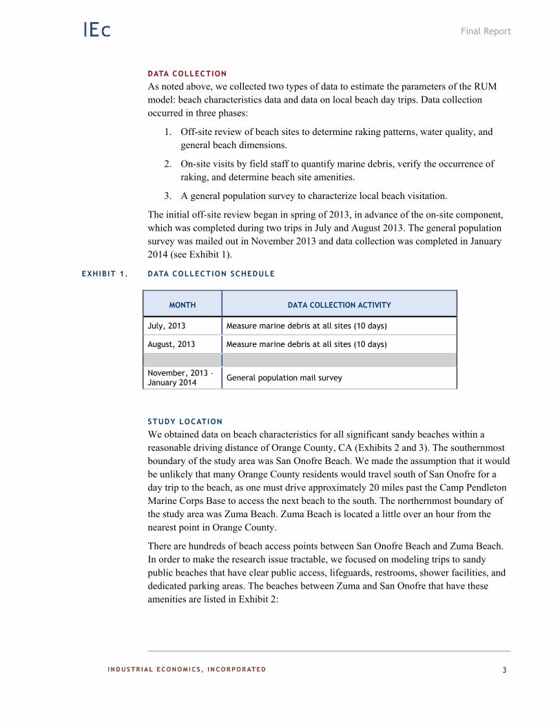
The initial off-site review began in spring of 2013, in advance of the on-site component, which was completed during two trips in July and August 2013. The general population survey was mailed out in November 2013 and data collection was completed in January 2014 (see Exhibit 1).

EXHIBIT 1. DATA COLLECTION SCHEDULE

MONTH DATA COLLECTION ACTIVITY

July, 2013 Measure marine debris at all sites (10 days)

August, 2013 Measure marine debris at all sites (10 days)

November, 2013 – January 2014 General population mail survey

STUDY LOCATION

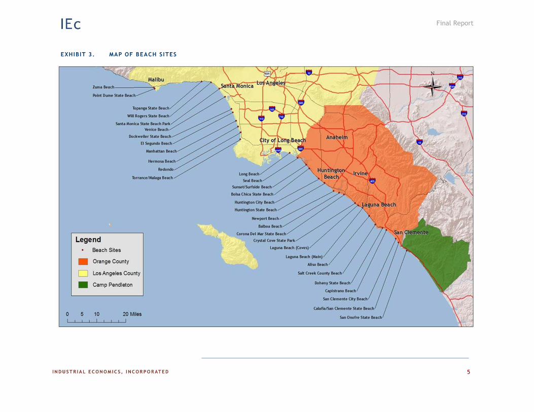
We obtained data on beach characteristics for all significant sandy beaches within a reasonable driving distance of Orange County, CA (Exhibits 2 and 3). The southernmost boundary of the study area was San Onofre Beach. We made the assumption that it would be unlikely that many Orange County residents would travel south of San Onofre for a day trip to the beach, as one must drive approximately 20 miles past the Camp Pendleton Marine Corps Base to access the next beach to the south. The northernmost boundary of the study area was Zuma Beach. Zuma Beach is located a little over an hour from the nearest point in Orange County.

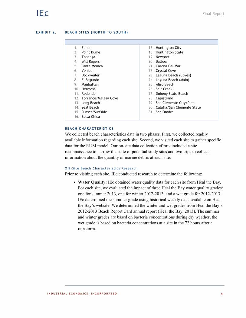
There are hundreds of beach access points between San Onofre Beach and Zuma Beach. In order to make the research issue tractable, we focused on modeling trips to sandy public beaches that have clear public access, lifeguards, restrooms, shower facilities, and dedicated parking areas. The beaches between Zuma and San Onofre that have these amenities are listed in Exhibit 2:

Final Report

4

EXHIBIT 2. BEACH SITES (NORTH TO SOUTH)

1. Zuma 2. Point Dume 3. Topanga 4. Will Rogers 5. Santa Monica 6. Venice 7. Dockweiler 8. El Segundo 9. Manhattan 10. Hermosa 11. Redondo 12. Torrance/Malaga Cove 13. Long Beach 14. Seal Beach 15. Sunset/Surfside 16. Bolsa Chica

17. Huntington City 18. Huntington State 19. Newport 20. Balboa 21. Corona Del Mar 22. Crystal Cove 23. Laguna Beach (Coves) 24. Laguna Beach (Main) 25. Aliso Beach 26. Salt Creek 27. Doheny State Beach 28. Capistrano 29. San Clemente City/Pier 30. Calafia/San Clemente State 31. San Onofre

BEACH CHARACTERISTICS

We collected beach characteristics data in two phases. First, we collected readily available information regarding each site. Second, we visited each site to gather specific data for the RUM model. Our on-site data collection efforts included a site reconnaissance to narrow the suite of potential study sites and two trips to collect information about the quantity of marine debris at each site.

Off -S i te Beach Character i s t i c s Research

Prior to visiting each site, IEc conducted research to determine the following:

Water Quality: IEc obtained water quality data for each site from Heal the Bay. For each site, we evaluated the impact of three Heal the Bay water quality grades: one for summer 2013, one for winter 2012-2013, and a wet grade for 2012-2013. IEc determined the summer grade using historical weekly data available on Heal the Bay’s website. We determined the winter and wet grades from Heal the Bay’s 2012-2013 Beach Report Card annual report (Heal the Bay, 2013). The summer and winter grades are based on bacteria concentrations during dry weather; the wet grade is based on bacteria concentrations at a site in the 72 hours after a rainstorm.

Final Report

5

EXHIBIT 3. MAP OF BEACH SITES

Final Report

6

Raking: Many of the larger beaches are raked daily with mechanical equipment to minimize refuse and provide a smooth surface for recreation. We contacted the managers of each beach to ascertain whether the beach is raked and how frequently.

Beach Length & Shoreline Characteristics: We calculated the length of each shoreline site using coordinates collected on-site and satellite imagery. We also determined the nearest towns, nearest rivers, aspect and location/major usage for each site. These data were verified by the field staff once on-site. IEc also calculated the tidal range by locating the nearest tidal gauge for each site, downloading the ranges for the study period, and calculating the distance between the highest high tide and lowest low tide (U.S. DOC, 2013).

Sample Transect Selection: To characterize debris at each beach, IEc randomly selected sampling locations (transects) prior to arriving on-site. At each sampling location, IEc randomly selected four transects for debris characterization. For each transect, we filled out the “Transect #” and “Transect Range” fields on the sampling site characterization sheet (Appendix A). Doing this in advance of each site visit allowed the field staff to quickly flag the pre-determined transects during the initial site set-up.

On-S ite Beach Character ist ics Col lect ion

We obtained data on beach characteristics primarily through on-site observations and measurements during two periods: July 9, 2013 to July 15, 2013 and August 13, 2013 to August 20, 2013. During these site visits, we collected data on the following characteristics:

Beach Width: We measured beach width on site from the water line to the back of the beach using a GPS unit. The measurement was taken at the entrance to the beach from the main parking lot. If there were multiple entrances to the beach from the main parking lot, then width was measured at the midpoint between the outer entrances. We later calculated the distance between these points using the coordinates recorded by the GPS unit.

Beach Amenities: We recorded the presence/absence of the following amenities: volleyball nets, fire pits, piers, a bike path/boardwalk, food concessions, and playgrounds.

Type of Neighborhood: We recorded whether the neighborhood adjacent to the beach was primarily urban, suburban, or rural. To validate our on-site observations, we used US Census data to determine whether a site was in an urban or rural census block (U.S. Census Bureau, 2013). We re-classified sites that fell in a rural census block as rural. If the site was in an urban block, we evaluated whether the site fell within a principal city. We classified sites within a principal city as urban and sites outside of the principal city as suburban.

Final Report

7

Parking Cost: We calculated the cost of parking for an eight hour period in the beach parking lot.

Cobbles: We noted whether or not the beach had areas where the sand has washed away and large cobbles remain (i.e., larger than four inches in diameter).

Beach Raking: During the on-site visit, field staff documented whether raking had occurred in the beach study area at the time of data collection.

Marine Debris: Field staff measured and recorded the amount of marine debris as described below.

We obtained marine debris data through detailed measurements at each site using methods similar to those specified in NOAA’s Marine Debris Shoreline Survey Field Guide (Opfer et al. 2012) for standing stock studies. Please see the debris characterization handbook in Appendix B for detailed instructions, protocols, and forms used by field staff.

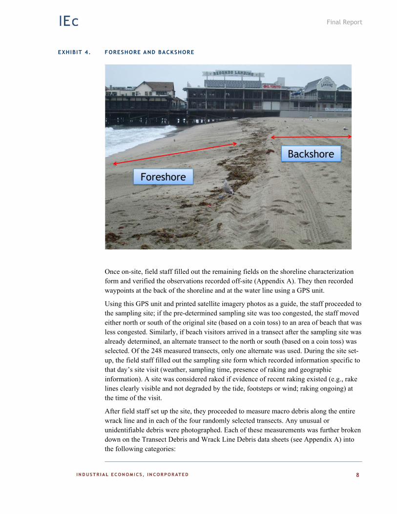
During each assessment, field personnel counted and categorized all observed macro debris (debris larger than 2.5 cm on the longest dimension) along the four randomly selected 5m wide transects within a 100m segment of beach.2 Each transect spanned the beach from water’s edge to the back of the shoreline and was divided into two sections for counting purposes, the “foreshore” and the “backshore.” The foreshore is defined as the section of beach “which lies between high and low water mark at ordinary tide” (IHO 1994). It is the steeply-sloped section of the beach where waves wash up (Exhibit 4). The backshore is defined as the mildly-sloped or flat section of beach “which is usually dry, being reached only by the highest tides (IHO 1994).3 At most beaches in the study area, the backshore is regularly raked, so there is minimal, if any wrack in the backshore area. However, at beaches that are not regularly raked, wrack can occur in both the foreshore and the backshore areas.

2 Field personnel did not measure micro debris, as it was not expected to have a significant impact on the behavior of beach visitors.

3 Some authors (e.g., Ellis 1978) refer to the backshore as the “berm” and use the term “berm crest” to describe the boundary between the foreshore and backshore.

Final Report

8

EXHIBIT 4. FORESHORE AND BACKSHORE

Once on-site, field staff filled out the remaining fields on the shoreline characterization form and verified the observations recorded off-site (Appendix A). They then recorded waypoints at the back of the shoreline and at the water line using a GPS unit.

Using this GPS unit and printed satellite imagery photos as a guide, the staff proceeded to the sampling site; if the pre-determined sampling site was too congested, the staff moved either north or south of the original site (based on a coin toss) to an area of beach that was less congested. Similarly, if beach visitors arrived in a transect after the sampling site was already determined, an alternate transect to the north or south (based on a coin toss) was selected. Of the 248 measured transects, only one alternate was used. During the site set-up, the field staff filled out the sampling site form which recorded information specific to that day’s site visit (weather, sampling time, presence of raking and geographic information). A site was considered raked if evidence of recent raking existed (e.g., rake lines clearly visible and not degraded by the tide, footsteps or wind; raking ongoing) at the time of the visit.

After field staff set up the site, they proceeded to measure macro debris along the entire wrack line and in each of the four randomly selected transects. Any unusual or unidentifiable debris were photographed. Each of these measurements was further broken down on the Transect Debris and Wrack Line Debris data sheets (see Appendix A) into the following categories:

Final Report

9

1. Plastics – plastic fragments (hard, foamed, film), food wrappers, beverage bottles/containers, bottle caps, cigar tips, cigarettes, disposable lighters, 6-pack rings, bags, rope/net, buoys/floats, fishing lure/line, cups, utensils, straws, balloons, personal care products.

2. Metals – aluminum cans, aerosol cans, metal fragments.

3. Glass – beverage bottles, jars, glass fragments.

4. Rubber – flip-flops, gloves, tires, rubber fragments.

5. Processed Lumber – cardboard cartons, paper and cardboard, paper bags, lumber/building material.

6. Cloth/Fabrics – clothing/shoes, gloves (non-rubber), towels/rags, rope/net pieces (non-nylon), fabric pieces.

7. Other/Unclassifiable – food, etc.

8. Large Debris- items greater than one foot in longest dimension.

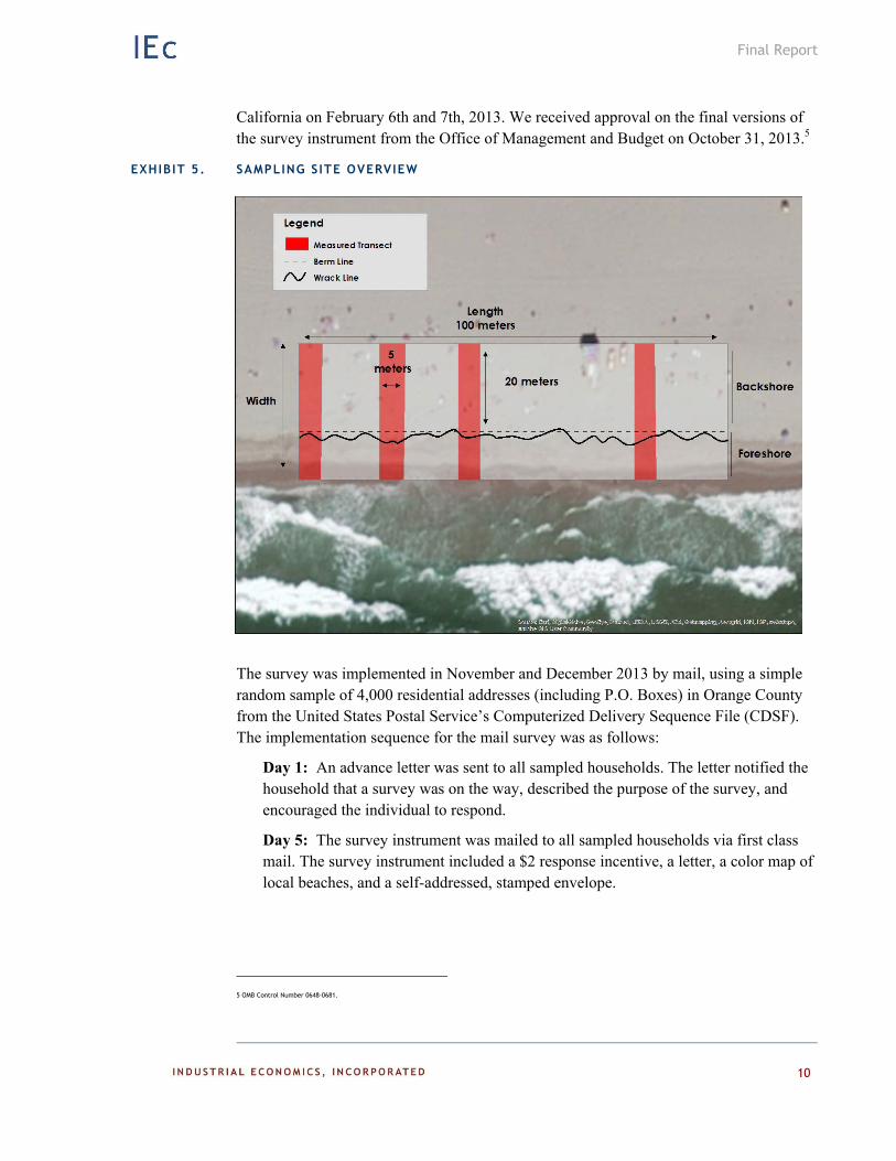
For the wrack line measurements, the field staff followed the wrack line from the northern or southern edge of the sampling site to the opposite edge, a distance of 100 meters. Along this distance, debris was measured if it fell within 2 meters of the center of the wrack line. In areas with no wrack line present, the field staff followed the berm line.

For the transect measurements, the field staff flagged each transect prior to debris characterization using two 20 meter rope-lines for the backshore and a rope spool for the foreshore. Each transect extended from the water’s edge up to 20 meters past the berm line4 and was 5 meters long (Exhibit 5). Transect widths ranged from 13.5 meters at San Onofre State Beach to 64 meters at Seal Beach. The longest transect widths were recorded at beaches with long, gradually sloping foreshores.

LOCAL BEACH DAY TRIPS DATA

Data on beach visits were obtained through a general population mail survey of Orange County households. The survey included questions that focused on beach day trips, beach activities, marine debris at local beaches, and demographic characteristics (see survey instrument in Appendix C). The survey also asked respondents to indicate how important certain beach characteristics are when deciding to visit local beaches and level of concern with debris on beaches. With regard to beach day trips, the respondent was asked to indicate the specific local beaches that he or she visited in June, July and August of 2013 and the number of day trips taken, by month, to each location. We pre-tested draft versions of the survey through two focus groups (nine participants total) in Irvine,

4 Field staff measured up to 20 meters past the berm line; however, if the beach ended (i.e., field staff reached the parking

lot) before 20 meters, they stopped at the beach’s edge.

Final Report

10

California on February 6th and 7th, 2013. We received approval on the final versions of the survey instrument from the Office of Management and Budget on October 31, 2013.5

EXHIBIT 5. SAMPLING S ITE OVERVIEW

The survey was implemented in November and December 2013 by mail, using a simple random sample of 4,000 residential addresses (including P.O. Boxes) in Orange County from the United States Postal Service’s Computerized Delivery Sequence File (CDSF). The implementation sequence for the mail survey was as follows:

Day 1: An advance letter was sent to all sampled households. The letter notified the household that a survey was on the way, described the purpose of the survey, and encouraged the individual to respond.

Day 5: The survey instrument was mailed to all sampled households via first class mail. The survey instrument included a $2 response incentive, a letter, a color map of local beaches, and a self-addressed, stamped envelope.

5 OMB Control Number 0648-0681.

Final Report

11

Day 12: A thank you/reminder postcard was mailed to all sampled households thanking them for responding and encouraging them to complete the survey if they hadn’t already.

Day 26: A replacement survey instrument was mailed to all sampled households who had not yet responded. The replacement survey included a letter, a color map and a self-addressed, stamped envelope.

To investigate the potential for non-response bias, we conducted a non-respondent follow-up mail survey with a sub-sample of 600 individuals who did not respond to the survey.6 To maximize the likelihood of response, the non-respondent follow-up survey was extremely short (five questions) and was sent via two-day Federal Express (Appendix D). The questions in the non-respondent follow-up survey were a subset of the questions from the main survey, selected to characterize non-respondents with respect to number of beach trips and attitude towards marine debris. No demographic questions were included on the non-respondent follow-up survey, as response bias associated with demographic characteristics can be adequately assessed by comparing demographic characteristics of respondents with county-level census data and using raking procedures if there are substantial differences. The non-response follow-up survey was implemented four weeks after the replacement survey was mailed.

SUMMARY RESULTS

Overall, we collected hundreds of data points on all 31 selected sites during our data collection efforts, as well as 18 measurements of marine debris at each site. We received 1,436 completed mail surveys, providing an overall response rate of 36.5 percent (AAPOR 3). In addition, we received 93 non-response follow-up surveys, providing a response rate of 15.6 percent.7

We used double data entry into an Access database for all beach characteristics data, and verified and corrected all discrepancies. We standardized all units and values in the data and text fields (e.g., converted miles to meters) to facilitate summary and analysis. We also calculated beach widths and transect widths using the waypoints collected during the on-site period and converted them to distances. The mail survey and non-response survey data were entered into an electronic database using double-key data entry, with any discrepancies evaluated and resolved.

6 Initially, we had planned to allocate half of the sample of 600 non-respondents to a phone survey mode. However a recent study comparing mail and phone follow-up surveys found the

telephone follow-up to be inferior to a mail follow-up implemented via FedEx (Han et al. 2010). This is at least partly due to the fact that phone numbers can be matched to only about 60

percent of the sampled addresses, and phone number matches cannot be obtained for cell-only households.

7 For the main survey, 4,001 surveys were mailed. There were 1,436 completed surveys, 66 undeliverable surveys (i.e., bad addresses), 39 explicit refusals, 3 returned but marked as ineligible

due to illness/health, and 2,457 surveys that were never returned. The main survey response rate is calculated as 0.365 = 1,436 ÷ (1,436 + 2,457 + 39). For the non-respondent follow-up survey,

600 surveys were mailed. There were 93 completed surveys, 4 undeliverable surveys, and 503 that were never returned. The follow-up survey response rate is calculated as 0.156 = 93 ÷ (93 +

503).

Final Report

12

BEACH CHARACTERISTICS

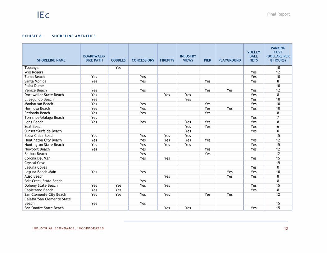
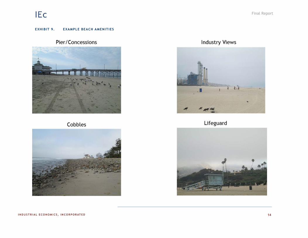
As noted above, we recorded the presence/absence of the following beach characteristics during our on-site visits: boardwalk/bike path, cobbles, concession, fire pits, piers, playgrounds, and volleyball nets. We also noted if there were views of industrial complexes from the beach, and we calculated the cost to park for a full day (i.e., eight hours) at the beach. Over half of the sites have a boardwalk or bike path (19 beaches); for example, the South Bay bike trail that extends from Santa Monica Beach to Redondo Beach. Very few beaches had evidence of cobbles (only four beaches). Concessions were also relatively available (18 beaches), but very few sites had playgrounds (five beaches). Parking costs range from free to $15 per day, with an average cost of $10 per day. Exhibit 8 summarizes the amenities for each beach, Exhibit 9 provides some examples of observed characteristics.

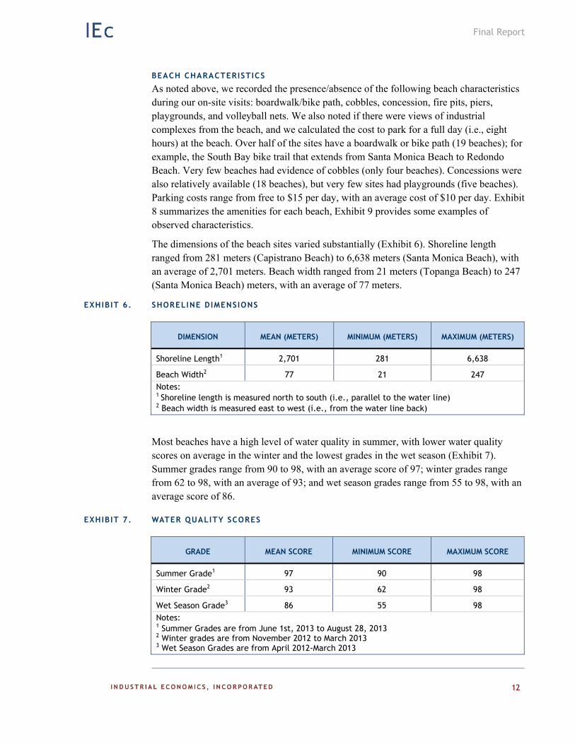
The dimensions of the beach sites varied substantially (Exhibit 6). Shoreline length ranged from 281 meters (Capistrano Beach) to 6,638 meters (Santa Monica Beach), with an average of 2,701 meters. Beach width ranged from 21 meters (Topanga Beach) to 247 (Santa Monica Beach) meters, with an average of 77 meters.

EXHIBIT 6. SHORELINE DIMENSIONS

DIMENSION MEAN (METERS) MINIMUM (METERS) MAXIMUM (METERS)

Shoreline Length1 2,701 281 6,638

Beach Width2 77 21 247 Notes: 1 Shoreline length is measured north to south (i.e., parallel to the water line) 2 Beach width is measured east to west (i.e., from the water line back)

Most beaches have a high level of water quality in summer, with lower water quality scores on average in the winter and the lowest grades in the wet season (Exhibit 7). Summer grades range from 90 to 98, with an average score of 97; winter grades range from 62 to 98, with an average of 93; and wet season grades range from 55 to 98, with an average score of 86.

EXHIBIT 7. WATER QUALITY SCORES

GRADE MEAN SCORE MINIMUM SCORE MAXIMUM SCORE

Summer Grade1 97 90 98

Winter Grade2 93 62 98

Wet Season Grade3 86 55 98 Notes: 1 Summer Grades are from June 1st, 2013 to August 28, 2013 2 Winter grades are from November 2012 to March 2013 3 Wet Season Grades are from April 2012-March 2013

Final Report

13

EXHIBIT 8. SHORELINE AMENITIES

SHORELINE NAME BOARDWALK/

BIKE PATH COBBLES CONCESSIONS FIREPITS INDUSTRY

VIEWS PIER PLAYGROUND

VOLLEY BALL NETS

PARKING COST

(DOLLARS PER 8 HOURS)

Topanga Yes 10 Will Rogers Yes 12 Zuma Beach Yes Yes Yes 10 Santa Monica Yes Yes Yes Yes 8 Point Dume 10 Venice Beach Yes Yes Yes Yes Yes 12 Dockweiler State Beach Yes Yes Yes Yes 8 El Segundo Beach Yes Yes Yes 10 Manhattan Beach Yes Yes Yes Yes 10 Hermosa Beach Yes Yes Yes Yes Yes 10 Redondo Beach Yes Yes Yes 8 Torrance/Malaga Beach Yes Yes 7 Long Beach Yes Yes Yes Yes Yes 8 Seal Beach Yes Yes Yes 6 Sunset/Surfside Beach Yes Yes 0 Bolsa Chica Beach Yes Yes Yes Yes 15 Huntington City Beach Yes Yes Yes Yes Yes Yes 12 Huntington State Beach Yes Yes Yes Yes Yes 15 Newport Beach Yes Yes Yes Yes 12 Balboa Beach Yes Yes 12 Corona Del Mar Yes Yes Yes 15 Crystal Cove 15 Laguna Coves Yes 0 Laguna Beach Main Yes Yes Yes Yes 10 Aliso Beach Yes Yes Yes 8 Salt Creek State Beach Yes 8 Doheny State Beach Yes Yes Yes Yes Yes 15 Capistrano Beach Yes Yes Yes 8 San Clemente City Beach Yes Yes Yes Yes Yes Yes 12 Calafia/San Clemente State Beach Yes Yes 15 San Onofre State Beach Yes Yes Yes 15

Final Report

14

EXHIBIT 9. EXAMPLE BEACH AMENITIES

Final Report

15

Marine Debr is

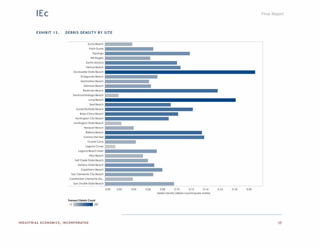
Overall, we found that marine debris varied greatly between sites, both in terms of total debris counts, and in total debris density. To account for transects with larger areas, we calculated the debris density as the total debris count divided by the transect area.8 Exhibit 13 below displays both the total debris count and debris density by site. In general, sites with a large total debris count also had a high debris density.

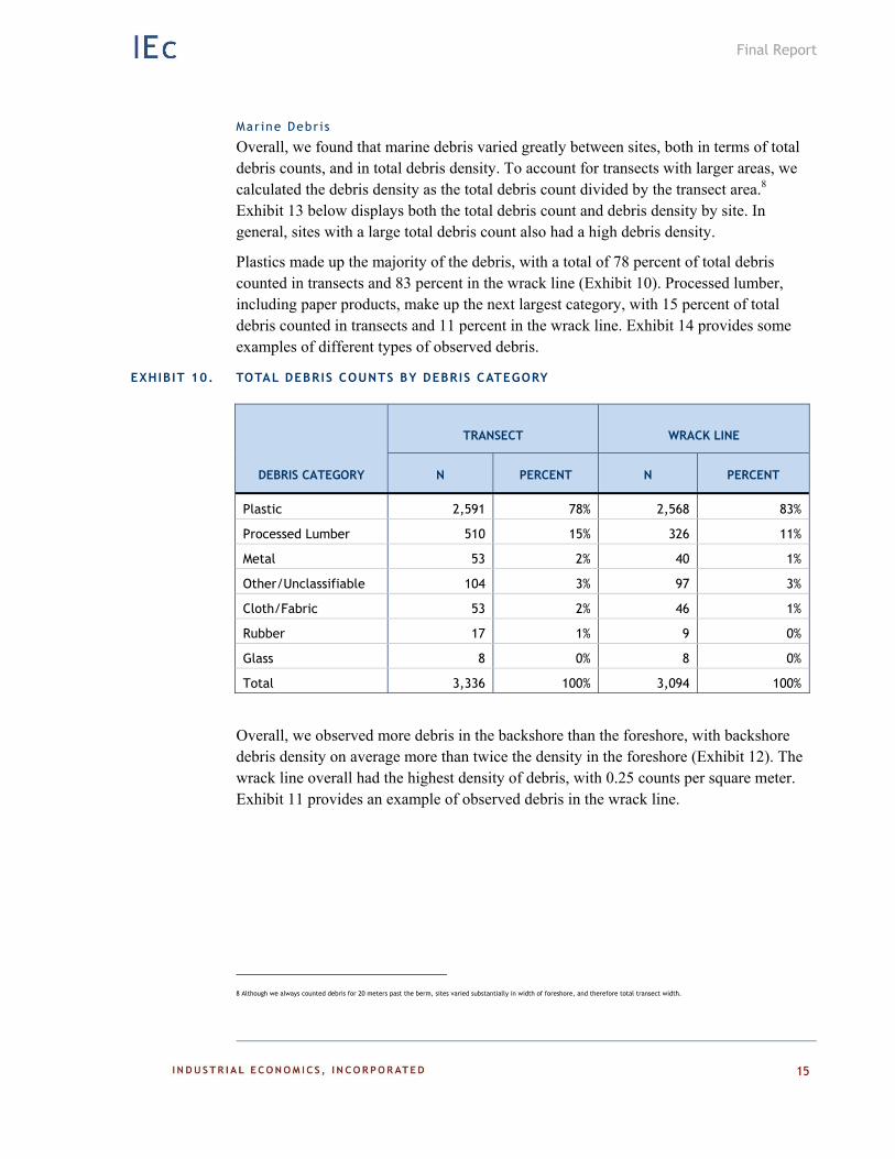
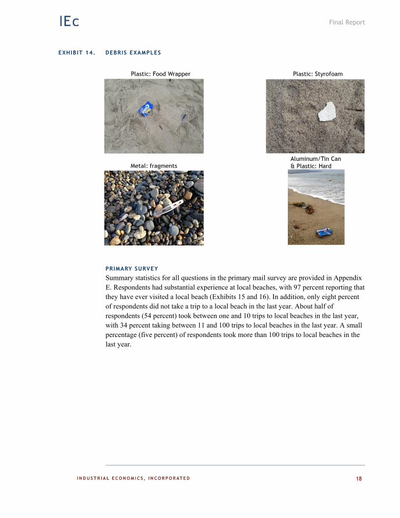
Plastics made up the majority of the debris, with a total of 78 percent of total debris counted in transects and 83 percent in the wrack line (Exhibit 10). Processed lumber, including paper products, make up the next largest category, with 15 percent of total debris counted in transects and 11 percent in the wrack line. Exhibit 14 provides some examples of different types of observed debris.

EXHIBIT 10. TOTAL DEBRIS COUNTS BY DEBRIS CATEGORY

DEBRIS CATEGORY

TRANSECT WRACK LINE

N PERCENT N PERCENT

Plastic 2,591 78% 2,568 83%

Processed Lumber 510 15% 326 11%

Metal 53 2% 40 1%

Other/Unclassifiable 104 3% 97 3%

Cloth/Fabric 53 2% 46 1%

Rubber 17 1% 9 0%

Glass 8 0% 8 0%

Total 3,336 100% 3,094 100%

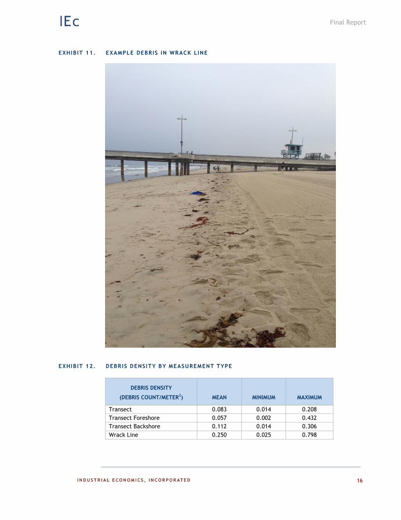
Overall, we observed more debris in the backshore than the foreshore, with backshore debris density on average more than twice the density in the foreshore (Exhibit 12). The wrack line overall had the highest density of debris, with 0.25 counts per square meter. Exhibit 11 provides an example of observed debris in the wrack line.

8 Although we always counted debris for 20 meters past the berm, sites varied substantially in width of foreshore, and therefore total transect width.

Final Report

16

EXHIBIT 11. EXAMPLE DEBRIS IN WRACK LINE

EXHIBIT 12. DEBRIS DENSITY BY MEASUREMENT TYPE

DEBRIS DENSITY

(DEBRIS COUNT/METER2) MEAN MINIMUM MAXIMUM

Transect 0.083 0.014 0.208 Transect Foreshore 0.057 0.002 0.432 Transect Backshore 0.112 0.014 0.306 Wrack Line 0.250 0.025 0.798

Final Report

17

EXHIBIT 13. DEBRIS DENSITY BY S ITE

0.00 0.02 0.04 0.06 0.08 0.10 0.12 0.14 0.16 0.18 0.20Debris Density (debris count/square meter)

Zuma Beach

Point Dume

Topanga

Will Rogers

Santa Monica

Venice Beach

Dockweiler State Beach

El Segundo Beach

Manhattan Beach

Hermosa Beach

Redondo Beach

Torrance/Malaga Beach

Long Beach

Seal Beach

Sunset/Surfside Beach

Bolsa Chica Beach

Huntington City Beach

Huntington State Beach

Newport Beach

Balboa Beach

Corona Del Mar

Crystal Cove

Laguna Coves

Laguna Beach Main

Aliso Beach

Salt Creek State Beach

Doheny State Beach

Capistrano Beach

San Clemente City Beach

Calafia/San Clemente Sta..

San Onofre State Beach

12 287Transect Debris Count

Final Report

18

EXHIBIT 14. DEBRIS EXAMPLES

PRIMARY SURVEY

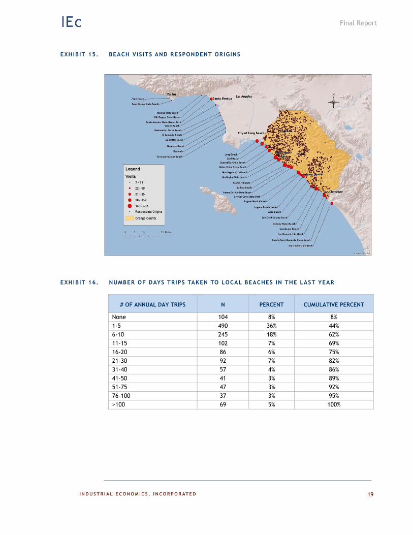
Summary statistics for all questions in the primary mail survey are provided in Appendix E. Respondents had substantial experience at local beaches, with 97 percent reporting that they have ever visited a local beach (Exhibits 15 and 16). In addition, only eight percent of respondents did not take a trip to a local beach in the last year. About half of respondents (54 percent) took between one and 10 trips to local beaches in the last year, with 34 percent taking between 11 and 100 trips to local beaches in the last year. A small percentage (five percent) of respondents took more than 100 trips to local beaches in the last year.

Final Report

19

EXHIBIT 15. BEACH VIS ITS AND RESPONDENT ORIGINS

EXHIBIT 16. NUMBER OF DAYS TRIPS TAKEN TO LOCAL BEACHES IN THE LAST YEAR

# OF ANNUAL DAY TRIPS N PERCENT CUMULATIVE PERCENT

None 104 8% 8% 1-5 490 36% 44% 6-10 245 18% 62% 11-15 102 7% 69% 16-20 86 6% 75% 21-30 92 7% 82% 31-40 57 4% 86% 41-50 41 3% 89% 51-75 47 3% 92% 76-100 37 3% 95% >100 69 5% 100%

Final Report

20

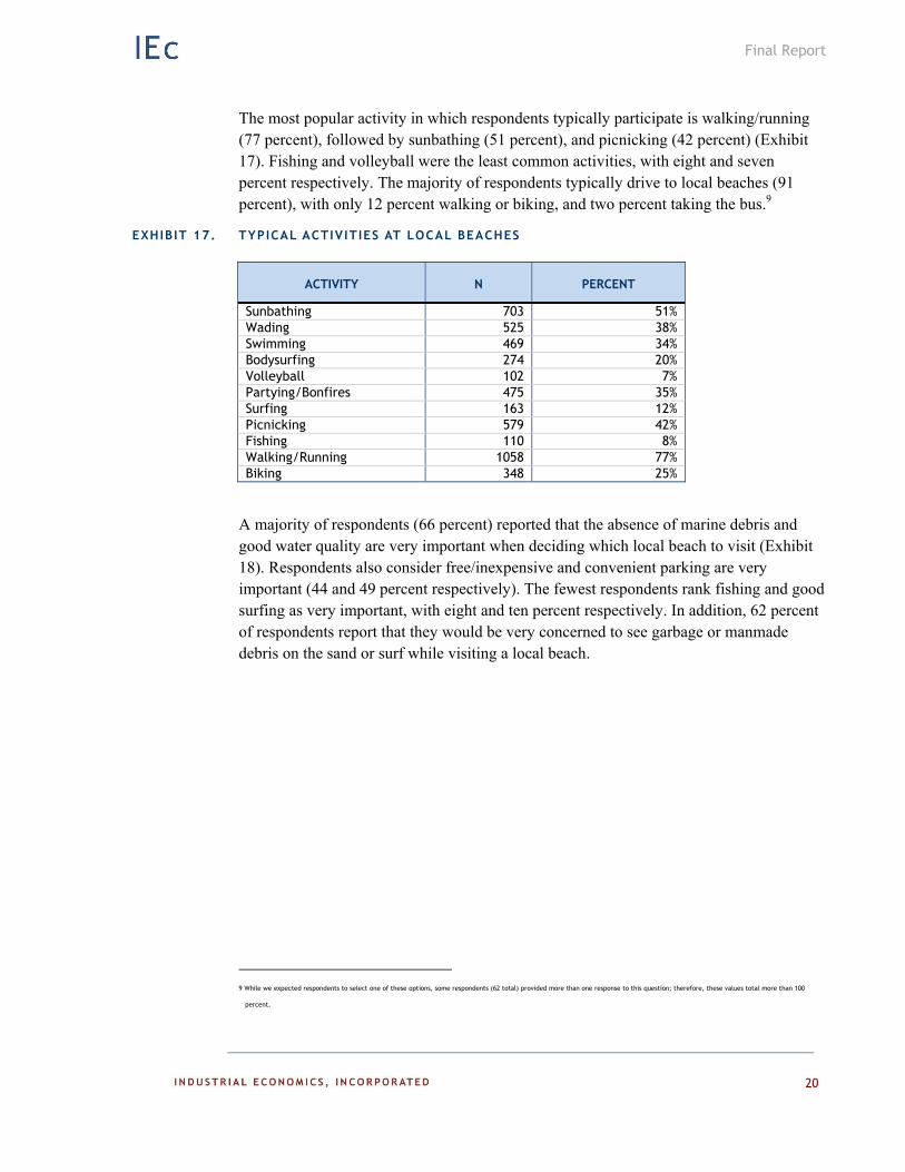
The most popular activity in which respondents typically participate is walking/running (77 percent), followed by sunbathing (51 percent), and picnicking (42 percent) (Exhibit 17). Fishing and volleyball were the least common activities, with eight and seven percent respectively. The majority of respondents typically drive to local beaches (91 percent), with only 12 percent walking or biking, and two percent taking the bus.9

EXHIBIT 17. TYPICAL ACTIVITIES AT LOCAL BEACHES

ACTIVITY N PERCENT

Sunbathing 703 51% Wading 525 38% Swimming 469 34% Bodysurfing 274 20% Volleyball 102 7% Partying/Bonfires 475 35% Surfing 163 12% Picnicking 579 42% Fishing 110 8% Walking/Running 1058 77% Biking 348 25%

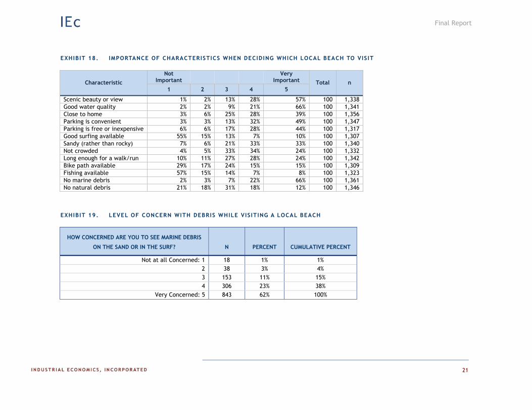
A majority of respondents (66 percent) reported that the absence of marine debris and good water quality are very important when deciding which local beach to visit (Exhibit 18). Respondents also consider free/inexpensive and convenient parking are very important (44 and 49 percent respectively). The fewest respondents rank fishing and good surfing as very important, with eight and ten percent respectively. In addition, 62 percent of respondents report that they would be very concerned to see garbage or manmade debris on the sand or surf while visiting a local beach.

9 While we expected respondents to select one of these options, some respondents (62 total) provided more than one response to this question; therefore, these values total more than 100

percent.

Final Report

21

EXHIBIT 18. IMPORTANCE OF CHARACTERISTICS WHEN DECIDING WHICH LOCAL BEACH TO VIS IT

Characteristic

Not Important Very

Important Total n 1 2 3 4 5

Scenic beauty or view 1% 2% 13% 28% 57% 100 1,338 Good water quality 2% 2% 9% 21% 66% 100 1,341 Close to home 3% 6% 25% 28% 39% 100 1,356 Parking is convenient 3% 3% 13% 32% 49% 100 1,347 Parking is free or inexpensive 6% 6% 17% 28% 44% 100 1,317 Good surfing available 55% 15% 13% 7% 10% 100 1,307 Sandy (rather than rocky) 7% 6% 21% 33% 33% 100 1,340 Not crowded 4% 5% 33% 34% 24% 100 1,332 Long enough for a walk/run 10% 11% 27% 28% 24% 100 1,342 Bike path available 29% 17% 24% 15% 15% 100 1,309 Fishing available 57% 15% 14% 7% 8% 100 1,323 No marine debris 2% 3% 7% 22% 66% 100 1,361 No natural debris 21% 18% 31% 18% 12% 100 1,346

EXHIBIT 19. LEVEL OF CONCERN WITH DEBRIS WHILE VIS IT ING A LOCAL BEACH

HOW CONCERNED ARE YOU TO SEE MARINE DEBRIS

ON THE SAND OR IN THE SURF? N PERCENT CUMULATIVE PERCENT

Not at all Concerned: 1 18 1% 1% 2 38 3% 4% 3 153 11% 15% 4 306 23% 38%

Very Concerned: 5 843 62% 100%

Final Report

22

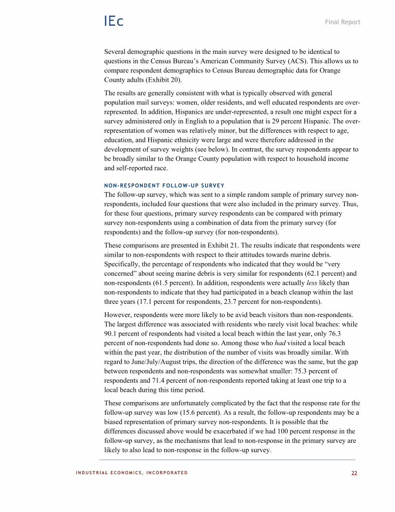
Several demographic questions in the main survey were designed to be identical to questions in the Census Bureau’s American Community Survey (ACS). This allows us to compare respondent demographics to Census Bureau demographic data for Orange County adults (Exhibit 20).

The results are generally consistent with what is typically observed with general population mail surveys: women, older residents, and well educated respondents are over-represented. In addition, Hispanics are under-represented, a result one might expect for a survey administered only in English to a population that is 29 percent Hispanic. The over-representation of women was relatively minor, but the differences with respect to age, education, and Hispanic ethnicity were large and were therefore addressed in the development of survey weights (see below). In contrast, the survey respondents appear to be broadly similar to the Orange County population with respect to household income and self-reported race.

NON-RESPONDENT FOLLOW-UP SURVEY

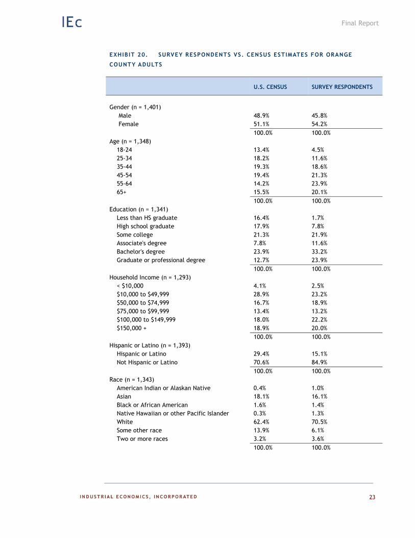
The follow-up survey, which was sent to a simple random sample of primary survey non-respondents, included four questions that were also included in the primary survey. Thus, for these four questions, primary survey respondents can be compared with primary survey non-respondents using a combination of data from the primary survey (for respondents) and the follow-up survey (for non-respondents).

These comparisons are presented in Exhibit 21. The results indicate that respondents were similar to non-respondents with respect to their attitudes towards marine debris. Specifically, the percentage of respondents who indicated that they would be “very concerned” about seeing marine debris is very similar for respondents (62.1 percent) and non-respondents (61.5 percent). In addition, respondents were actually less likely than non-respondents to indicate that they had participated in a beach cleanup within the last three years (17.1 percent for respondents, 23.7 percent for non-respondents).

However, respondents were more likely to be avid beach visitors than non-respondents. The largest difference was associated with residents who rarely visit local beaches: while 90.1 percent of respondents had visited a local beach within the last year, only 76.3 percent of non-respondents had done so. Among those who had visited a local beach within the past year, the distribution of the number of visits was broadly similar. With regard to June/July/August trips, the direction of the difference was the same, but the gap between respondents and non-respondents was somewhat smaller: 75.3 percent of respondents and 71.4 percent of non-respondents reported taking at least one trip to a local beach during this time period.

These comparisons are unfortunately complicated by the fact that the response rate for the follow-up survey was low (15.6 percent). As a result, the follow-up respondents may be a biased representation of primary survey non-respondents. It is possible that the differences discussed above would be exacerbated if we had 100 percent response in the follow-up survey, as the mechanisms that lead to non-response in the primary survey are likely to also lead to non-response in the follow-up survey.

Final Report

23

EXHIBIT 20. SURVEY RESPONDENTS VS. CENSUS ESTIMATES FOR ORANGE

COUNTY ADULTS

U.S. CENSUS SURVEY RESPONDENTS

Gender (n = 1,401)

Male 48.9% 45.8% Female 51.1% 54.2% 100.0% 100.0% Age (n = 1,348) 18-24 13.4% 4.5% 25-34 18.2% 11.6% 35-44 19.3% 18.6% 45-54 19.4% 21.3% 55-64 14.2% 23.9% 65+ 15.5% 20.1% 100.0% 100.0% Education (n = 1,341) Less than HS graduate 16.4% 1.7% High school graduate 17.9% 7.8% Some college 21.3% 21.9% Associate's degree 7.8% 11.6% Bachelor's degree 23.9% 33.2% Graduate or professional degree 12.7% 23.9% 100.0% 100.0% Household Income (n = 1,293) < $10,000 4.1% 2.5% $10,000 to $49,999 28.9% 23.2% $50,000 to $74,999 16.7% 18.9% $75,000 to $99,999 13.4% 13.2% $100,000 to $149,999 18.0% 22.2% $150,000 + 18.9% 20.0% 100.0% 100.0% Hispanic or Latino (n = 1,393) Hispanic or Latino 29.4% 15.1% Not Hispanic or Latino 70.6% 84.9% 100.0% 100.0% Race (n = 1,343) American Indian or Alaskan Native 0.4% 1.0% Asian 18.1% 16.1% Black or African American 1.6% 1.4% Native Hawaiian or other Pacific Islander 0.3% 1.3% White 62.4% 70.5% Some other race 13.9% 6.1% Two or more races 3.2% 3.6% 100.0% 100.0%

Final Report

24

EXHIBIT 21. RESPONDENTS VS. NON-RESPONDENTS (MAIN SURVEY)

MAIN SURVEY NON-

RESPONDENTS

(N = 93)

MAIN SURVEY

RESPONDENTS

(N = 1,433)

Number of day trips to ocean beaches in the local area within the last year

None 23.7% 9.9% 1-10 40.9 52.3 11-20 8.6 13.4 21-30 3.2 6.6 31-40 4.3 4.1 41-50 4.3 2.9 50+ 15.1 10.9 100% 100% Number of day trips to ocean beaches in the local area in June, July, or August of 2013?

None 28.6% 24.7% 1-10 49.5 41.0 11-20 6.6 12.6 20+ 15.4 21.7 100% 100% Level of concern about seeing marine debris on the sand or in the surf (1 = Not concerned; 5 = Very concerned)

1 1.1% 1.3% 2 2.2 2.8 3 12.1 11.3 4 23.1 22.5 5 61.5 62.1 100% 100% Participated in a beach cleanup within the last three years?

YES 23.7% 17.1% NO 76.3 82.9 100% 100%

Final Report

25

RUM MODEL RESULTS

Model Overv iew

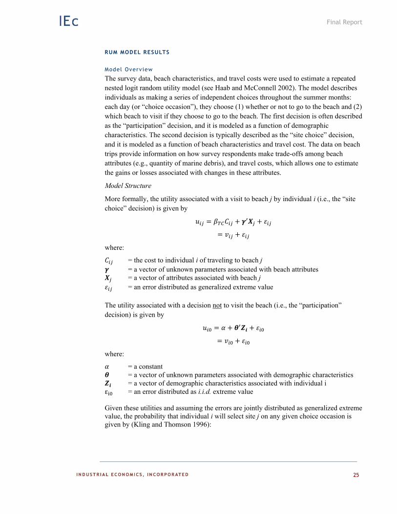
The survey data, beach characteristics, and travel costs were used to estimate a repeated nested logit random utility model (see Haab and McConnell 2002). The model describes individuals as making a series of independent choices throughout the summer months: each day (or “choice occasion”), they choose (1) whether or not to go to the beach and (2) which beach to visit if they choose to go to the beach. The first decision is often described as the “participation” decision, and it is modeled as a function of demographic characteristics. The second decision is typically described as the “site choice” decision, and it is modeled as a function of beach characteristics and travel cost. The data on beach trips provide information on how survey respondents make trade-offs among beach attributes (e.g., quantity of marine debris), and travel costs, which allows one to estimate the gains or losses associated with changes in these attributes.

Model Structure

More formally, the utility associated with a visit to beach j by individual i (i.e., the “site choice” decision) is given by

 

where:

= the cost to individual i of traveling to beach j = a vector of unknown parameters associated with beach attributes = a vector of attributes associated with beach j = an error distributed as generalized extreme value

The utility associated with a decision not to visit the beach (i.e., the “participation” decision) is given by

 

where:

= a constant = a vector of unknown parameters associated with demographic characteristics = a vector of demographic characteristics associated with individual i

ε = an error distributed as i.i.d. extreme value Given these utilities and assuming the errors are jointly distributed as generalized extreme value, the probability that individual i will select site j on any given choice occasion is given by (Kling and Thomson 1996):

Final Report

26

exp

expexp

exp exp

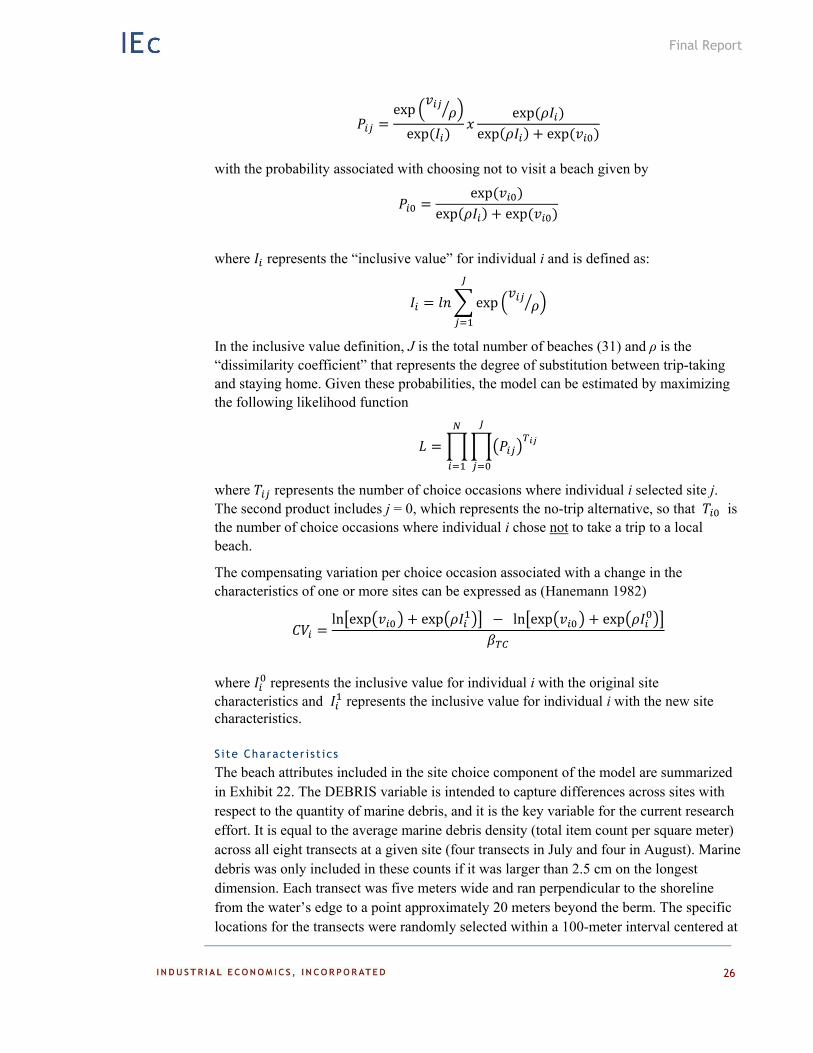
with the probability associated with choosing not to visit a beach given by

expexp exp

where represents the “inclusive value” for individual i and is defined as:

exp

In the inclusive value definition, J is the total number of beaches (31) and ρ is the “dissimilarity coefficient” that represents the degree of substitution between trip-taking and staying home. Given these probabilities, the model can be estimated by maximizing the following likelihood function

where represents the number of choice occasions where individual i selected site j. The second product includes j = 0, which represents the no-trip alternative, so that is the number of choice occasions where individual i chose not to take a trip to a local beach.

The compensating variation per choice occasion associated with a change in the characteristics of one or more sites can be expressed as (Hanemann 1982)

ln exp exp ln exp exp

where represents the inclusive value for individual i with the original site characteristics and represents the inclusive value for individual i with the new site characteristics.

S ite Character i st ics

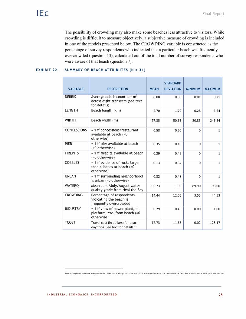
The beach attributes included in the site choice component of the model are summarized in Exhibit 22. The DEBRIS variable is intended to capture differences across sites with respect to the quantity of marine debris, and it is the key variable for the current research effort. It is equal to the average marine debris density (total item count per square meter) across all eight transects at a given site (four transects in July and four in August). Marine debris was only included in these counts if it was larger than 2.5 cm on the longest dimension. Each transect was five meters wide and ran perpendicular to the shoreline from the water’s edge to a point approximately 20 meters beyond the berm. The specific locations for the transects were randomly selected within a 100-meter interval centered at

Final Report

27

the entrance to the beach from the main parking lot. Additional details regarding marine debris measurements are provided in Appendix B.

The approximate size of the beach is captured by the LENGTH and WIDTH variables, both of which were measured using GIS. The width of the beach was measured near the main entrance.

Three binary (0/1) variables were included to capture the presence or absence of specific beach amenities: CONCESSION, PIER, and FIREPITS.10 The CONCESSION variable indicates whether a concession stand with food options was available at the beach. The PIER variable reflects the availability of a publicly accessible pier. The piers in this area are typically quite long and often offer concessions, restaurants, fishing opportunities, and other amenities. The FIREPITS variable reflects the availability of fire pits, which are designated locations where visitors can have bonfires, typically located at the back of the beach near the parking lot.

The binary COBBLES variable was included to capture the presence or absence of large (i.e., greater than 4 inches) cobbles that make it difficult to pursue typical beach activities. Although certain beaches are known to be more prone to cobbling than others, the extent of cobbling can vary both seasonally and spatially, depending on natural erosion and deposition patterns. The COBBLES variable reflects the presence or absence of cobbles on the stretch of beach where marine debris was measured.

As many survey respondents expressed concern about personal safety at beaches in open-ended responses, an attempt was made to identify crime data for the area. However, the available crime rate data did not vary adequately over space. As an alternative, a binary URBAN variable was included which reflected the land use surrounding each beach. This variable might capture differences in crime rates, but it may also capture additional driving costs (due to congestion) or the presence of additional amenities nearby such as restaurants and shops.

The WATERQ variable was included to capture differences across sites in the concentration of potentially harmful bacteria. Heal the Bay, a non-profit organization, publishes grades associated with weekly sampling events at beaches in Los Angeles and Orange County. The WATERQ variable represents the average of Heal the Bay’s weekly summer grades for each site.

Some of the beaches may be less attractive to visitors because power plants or other potentially unattractive structures are visible from the beach. This phenomenon was captured through a binary INDUSTRY variable, which is equal to one for beaches where there is a view of a power plant, offshore drilling platforms, airport, water treatment facility or other potential disamenity.

10 Although restrooms, lifeguards, showers, and parking are important beach amenities, they were not included in the model because all of the sites had these amenities.

Final Report

28

The possibility of crowding may also make some beaches less attractive to visitors. While crowding is difficult to measure objectively, a subjective measure of crowding is included in one of the models presented below. The CROWDING variable is constructed as the percentage of survey respondents who indicated that a particular beach was frequently overcrowded (question 13), calculated out of the total number of survey respondents who were aware of that beach (question 7).

EXHIBIT 22. SUMMARY OF BEACH ATTRIBUTES (N = 31)

VARIABLE DESCRIPTION MEAN

STANDARD

DEVIATION MINIMUM MAXIMUM

DEBRIS Average debris count per m2 across eight transects (see text for details)

0.08  0.05  0.01  0.21 

LENGTH Beach length (km)

2.70  1.70  0.28  6.64 

WIDTH Beach width (m)

77.35  50.66  20.83  246.84 

CONCESSIONS = 1 if concessions/restaurant available at beach (=0 otherwise)

0.58  0.50  0  1 

PIER = 1 if pier available at beach (=0 otherwise)

0.35  0.49  0  1 

FIREPITS = 1 if firepits available at beach (=0 otherwise)

0.29  0.46  0  1 

COBBLES = 1 if evidence of rocks larger than 4 inches at beach (=0 otherwise)

0.13  0.34  0  1 

URBAN = 1 if surrounding neighborhood is urban (=0 otherwise)

0.32  0.48  0  1 

WATERQ Mean June/July/August water quality grade from Heal the Bay

96.73  1.93  89.90  98.00 

CROWDING Percentage of respondents indicating the beach is frequently overcrowded

14.44  12.06  3.55  44.53 

INDUSTRY = 1 if view of power plant, oil platform, etc. from beach (=0 otherwise)

0.29  0.46  0.00  1.00 

TCOST Travel cost (in dollars) for beach day trips. See text for details.11 

17.73  11.65  0.02  128.17 

11 From the perspective of the survey respondent, travel cost is analogous to a beach attribute. The summary statistics for this variable are calculated across all 18,916 day trips to local beaches.

Final Report

29

Travel Cost

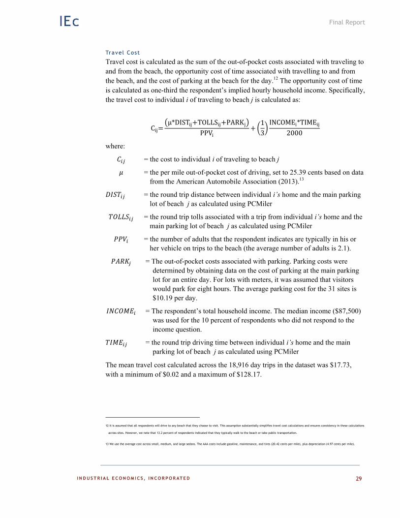
Travel cost is calculated as the sum of the out-of-pocket costs associated with traveling to and from the beach, the opportunity cost of time associated with travelling to and from the beach, and the cost of parking at the beach for the day.12 The opportunity cost of time is calculated as one-third the respondent’s implied hourly household income. Specifically, the travel cost to individual i of traveling to beach j is calculated as:

Cijμ*DISTij TOLLSij PARKj

PPVi

13

INCOMEi*TIMEij2000

where:

= the cost to individual i of traveling to beach j

= the per mile out-of-pocket cost of driving, set to 25.39 cents based on data from the American Automobile Association (2013).13

= the round trip distance between individual i’s home and the main parking lot of beach j as calculated using PCMiler

= the round trip tolls associated with a trip from individual i’s home and the main parking lot of beach j as calculated using PCMiler

= the number of adults that the respondent indicates are typically in his or her vehicle on trips to the beach (the average number of adults is 2.1).

= The out-of-pocket costs associated with parking. Parking costs were determined by obtaining data on the cost of parking at the main parking lot for an entire day. For lots with meters, it was assumed that visitors would park for eight hours. The average parking cost for the 31 sites is $10.19 per day.

= The respondent’s total household income. The median income ($87,500) was used for the 10 percent of respondents who did not respond to the income question.

  = the round trip driving time between individual i’s home and the main parking lot of beach j as calculated using PCMiler

The mean travel cost calculated across the 18,916 day trips in the dataset was $17.73, with a minimum of $0.02 and a maximum of $128.17.

12 It is assumed that all respondents will drive to any beach that they choose to visit. This assumption substantially simplifies travel cost calculations and ensures consistency in these calculations

across sites. However, we note that 13.2 percent of respondents indicated that they typically walk to the beach or take public transportation.

13 We use the average cost across small, medium, and large sedans. The AAA costs include gasoline, maintenance, and tires (20.42 cents per mile), plus depreciation (4.97 cents per mile).

Final Report

30

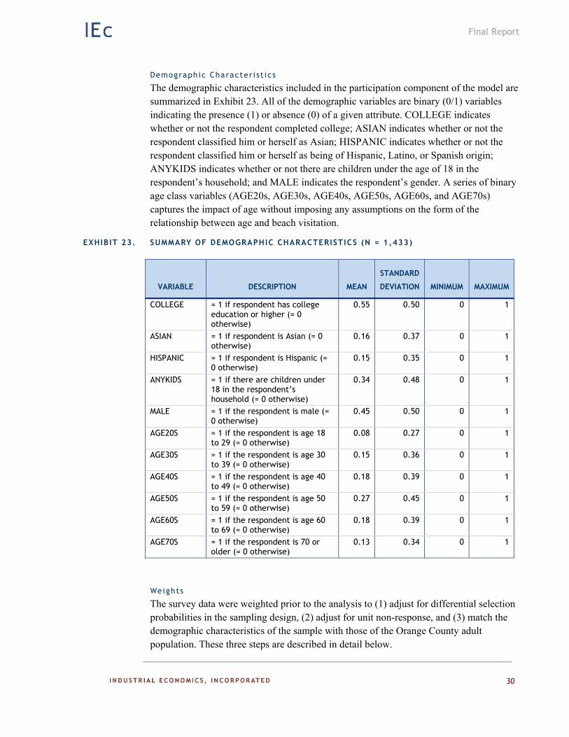
Demographic Character i st ics

The demographic characteristics included in the participation component of the model are summarized in Exhibit 23. All of the demographic variables are binary (0/1) variables indicating the presence (1) or absence (0) of a given attribute. COLLEGE indicates whether or not the respondent completed college; ASIAN indicates whether or not the respondent classified him or herself as Asian; HISPANIC indicates whether or not the respondent classified him or herself as being of Hispanic, Latino, or Spanish origin; ANYKIDS indicates whether or not there are children under the age of 18 in the respondent’s household; and MALE indicates the respondent’s gender. A series of binary age class variables (AGE20s, AGE30s, AGE40s, AGE50s, AGE60s, and AGE70s) captures the impact of age without imposing any assumptions on the form of the relationship between age and beach visitation.

EXHIBIT 23. SUMMARY OF DEMOGRAPHIC CHARACTERISTICS (N = 1,433)

VARIABLE DESCRIPTION MEAN

STANDARD

DEVIATION MINIMUM MAXIMUM

COLLEGE = 1 if respondent has college education or higher (= 0 otherwise)

0.55 0.50 0 1

ASIAN = 1 if respondent is Asian (= 0 otherwise)

0.16 0.37 0 1

HISPANIC = 1 if respondent is Hispanic (= 0 otherwise)

0.15 0.35 0 1

ANYKIDS = 1 if there are children under 18 in the respondent’s household (= 0 otherwise)

0.34 0.48 0 1

MALE = 1 if the respondent is male (= 0 otherwise)

0.45 0.50 0 1

AGE20S = 1 if the respondent is age 18 to 29 (= 0 otherwise)

0.08 0.27 0 1

AGE30S = 1 if the respondent is age 30 to 39 (= 0 otherwise)

0.15 0.36 0 1

AGE40S = 1 if the respondent is age 40 to 49 (= 0 otherwise)

0.18 0.39 0 1

AGE50S = 1 if the respondent is age 50 to 59 (= 0 otherwise)

0.27 0.45 0 1

AGE60S = 1 if the respondent is age 60 to 69 (= 0 otherwise)

0.18 0.39 0 1

AGE70S = 1 if the respondent is 70 or older (= 0 otherwise)

0.13 0.34 0 1

Weights

The survey data were weighted prior to the analysis to (1) adjust for differential selection probabilities in the sampling design, (2) adjust for unit non-response, and (3) match the demographic characteristics of the sample with those of the Orange County adult population. These three steps are described in detail below.

Final Report

31

The first step involved the development of a “base weight,” which is equal to the inverse of the selection probability for each respondent. There are 2,285,156 adults in Orange County in 2013, and 1,433 adults in our sample. Thus, if we had drawn a simple random sample of adults, the base weight would be 1,595, or 2,285,156 divided by 1,433. However, the sample design involved drawing a simple random sample of households, then randomly selecting a single adult from within each household. As a result, the selection probability for a given respondent is proportional to the inverse of the number of adults in his or her household. The base weights are therefore equal to the number of adults in the household times a constant that scales the sum of the weights to the population size, or 2,285,156.

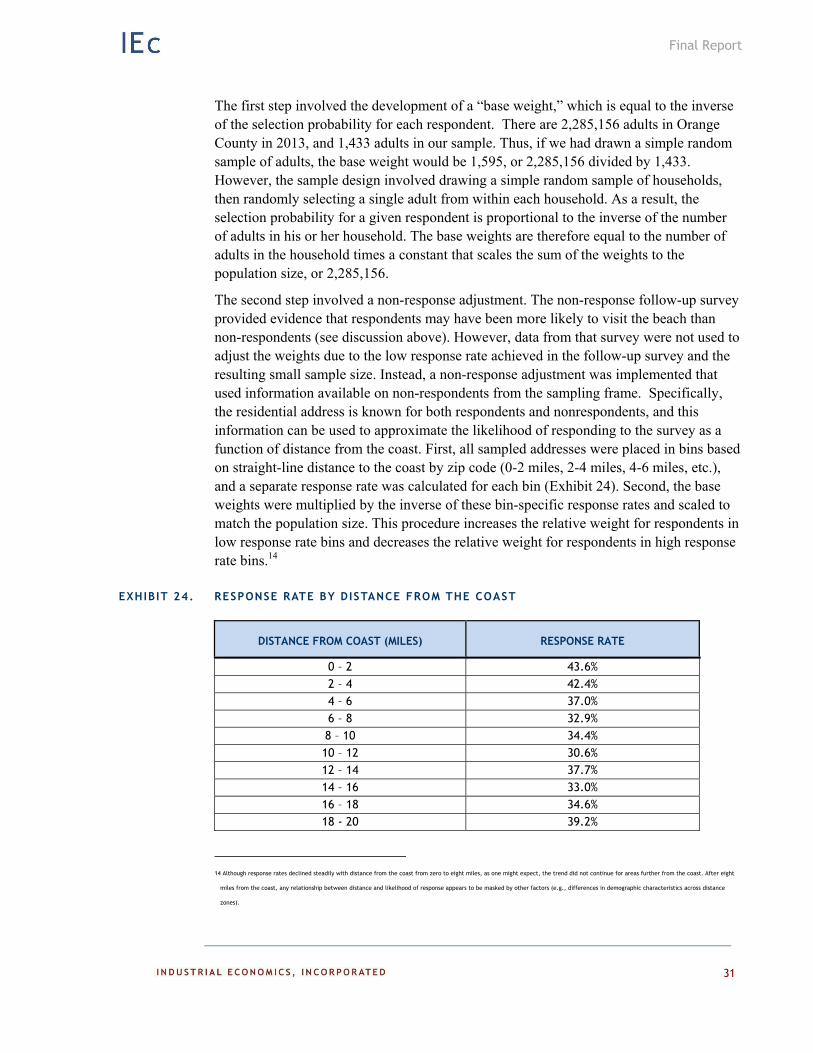
The second step involved a non-response adjustment. The non-response follow-up survey provided evidence that respondents may have been more likely to visit the beach than non-respondents (see discussion above). However, data from that survey were not used to adjust the weights due to the low response rate achieved in the follow-up survey and the resulting small sample size. Instead, a non-response adjustment was implemented that used information available on non-respondents from the sampling frame. Specifically, the residential address is known for both respondents and nonrespondents, and this information can be used to approximate the likelihood of responding to the survey as a function of distance from the coast. First, all sampled addresses were placed in bins based on straight-line distance to the coast by zip code (0-2 miles, 2-4 miles, 4-6 miles, etc.), and a separate response rate was calculated for each bin (Exhibit 24). Second, the base weights were multiplied by the inverse of these bin-specific response rates and scaled to match the population size. This procedure increases the relative weight for respondents in low response rate bins and decreases the relative weight for respondents in high response rate bins.14

EXHIBIT 24. RESPONSE RATE BY DISTANCE FROM THE COAST

DISTANCE FROM COAST (MILES) RESPONSE RATE

0 – 2 43.6% 2 – 4 42.4% 4 – 6 37.0% 6 – 8 32.9% 8 – 10 34.4% 10 – 12 30.6% 12 – 14 37.7% 14 – 16 33.0% 16 – 18 34.6% 18 - 20 39.2%

14 Although response rates declined steadily with distance from the coast from zero to eight miles, as one might expect, the trend did not continue for areas further from the coast. After eight

miles from the coast, any relationship between distance and likelihood of response appears to be masked by other factors (e.g., differences in demographic characteristics across distance

zones).

Final Report

32

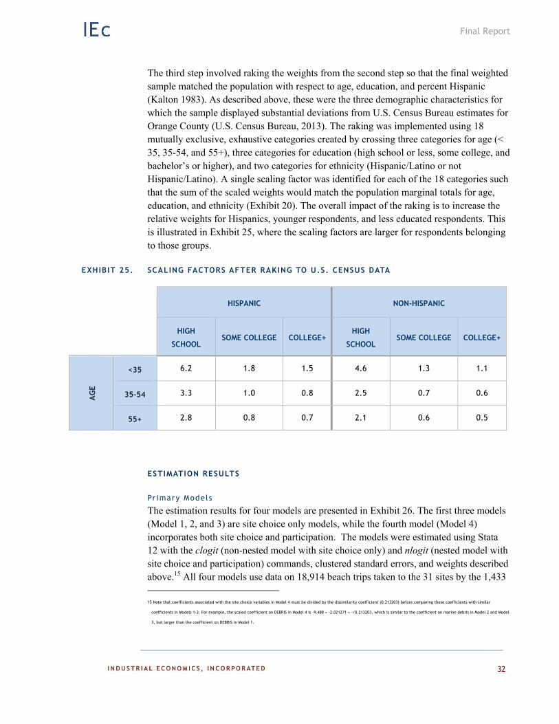
The third step involved raking the weights from the second step so that the final weighted sample matched the population with respect to age, education, and percent Hispanic (Kalton 1983). As described above, these were the three demographic characteristics for which the sample displayed substantial deviations from U.S. Census Bureau estimates for Orange County (U.S. Census Bureau, 2013). The raking was implemented using 18 mutually exclusive, exhaustive categories created by crossing three categories for age (< 35, 35-54, and 55+), three categories for education (high school or less, some college, and bachelor’s or higher), and two categories for ethnicity (Hispanic/Latino or not Hispanic/Latino). A single scaling factor was identified for each of the 18 categories such that the sum of the scaled weights would match the population marginal totals for age, education, and ethnicity (Exhibit 20). The overall impact of the raking is to increase the relative weights for Hispanics, younger respondents, and less educated respondents. This is illustrated in Exhibit 25, where the scaling factors are larger for respondents belonging to those groups.

EXHIBIT 25. SCALING FACTORS AFTER RAKING TO U.S. CENSUS DATA

HISPANIC NON-HISPANIC

HIGH

SCHOOL SOME COLLEGE COLLEGE+

HIGH

SCHOOL SOME COLLEGE COLLEGE+

AG

E

<35 6.2 1.8 1.5 4.6 1.3 1.1

35-54 3.3 1.0 0.8 2.5 0.7 0.6

55+ 2.8 0.8 0.7 2.1 0.6 0.5

ESTIMATION RESULTS

Pr imary Models

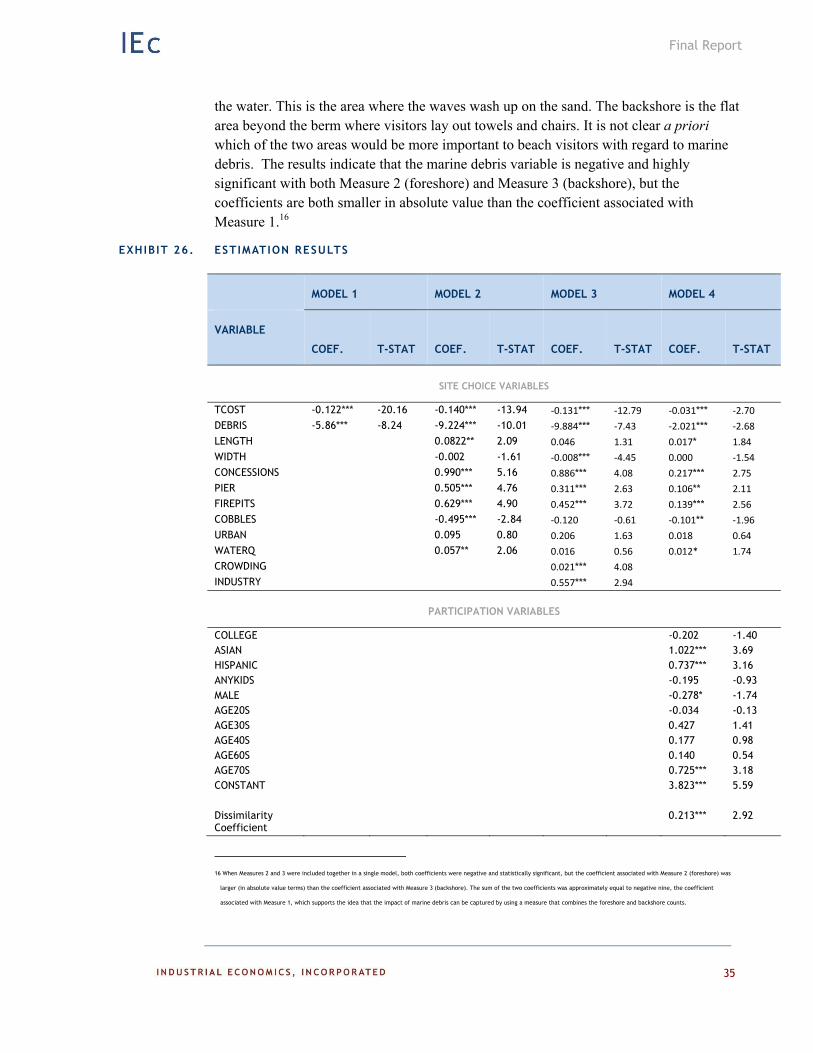
The estimation results for four models are presented in Exhibit 26. The first three models (Model 1, 2, and 3) are site choice only models, while the fourth model (Model 4) incorporates both site choice and participation. The models were estimated using Stata 12 with the clogit (non-nested model with site choice only) and nlogit (nested model with site choice and participation) commands, clustered standard errors, and weights described above.15 All four models use data on 18,914 beach trips taken to the 31 sites by the 1,433 15 Note that coefficients associated with the site choice variables in Model 4 must be divided by the dissimilarity coefficient (0.213203) before comparing these coefficients with similar

coefficients in Models 1-3. For example, the scaled coefficient on DEBRIS in Model 4 is -9.488 = -2.021271 = -/0.213203, which is similar to the coefficient on marine debris in Model 2 and Model

3, but larger than the coefficient on DEBRIS in Model 1.

Final Report

33

survey respondents. Model 4 uses 184 choice occasions in estimating the participation component of the model (two per day throughout June, July, and August).

Model 1 is an extremely simple model with only travel cost (TCOST) and marine debris (DEBRIS). Although this model has only minimal controls and is likely to suffer from omitted variable bias, it was nonetheless included to provide a general indication of the strength of the DEBRIS variable in explaining site choice before making decisions about the appropriate model specification.

Model 2 incorporates a set of objectively measured control variables in order to address omitted variables bias associated with Model 1, while Model 3 adds two subjectively measured, but potentially important, control variables, INDUSTRY, and CROWDING. Finally, Model 4 uses Model 2 (objective controls only) as a starting point and incorporates the participation decision in addition to the site choice decision.

As anticipated, the travel cost variable (TCOST) is negative and significant at the one percent level across all four models, indicating that respondents generally prefer beaches that are located closer to their homes. Marine debris (DEBRIS) is also negative and significant at the one percent level across all four models, indicating that respondents prefer to visit beaches that have less marine debris. This result proved to be quite robust to changes in model specification: the DEBRIS variable was consistently negative and significant across numerous model specifications.

The impact of beach size appears to be mixed. The coefficient on LENGTH is consistently positive, indicating that respondents prefer longer beaches, but it is significantly different from zero in only two of the three models where it was included (at the five percent level in one and at the ten percent level in the other). The coefficient on WIDTH is consistently negative but it is significant in only one of the three models. It is possible that some respondents prefer narrower beaches in the Orange County area, as many of the major beaches are extremely wide (seven were over one hundred meters wide) and the long walk to the water line from the parking lot may be onerous for some individuals.

The coefficients associated with the three amenity variables (CONCESSIONS, PIER, and FIREPITS) were all consistently positive and generally highly significant. The coefficient on CONCESSIONS was roughly twice as large as the coefficients on PIER and FIREPITS, indicating the importance of having food options available during beach visits.

The coefficient associated with COBBLES is negative and significant in two of the three models, and negative (but not significant) in the third. The coefficient associated with the URBAN variable is not statistically significant in any of the models.

The coefficient associated with water quality (WATERQ) is positive and significant (at the five and ten percent levels), as expected, in two of the models, and positive (but not significant) in the third. The absence of a strong, consistent water quality effect may

Final Report

34

simply reflect the fact that in the Orange County area, water quality (as measured by bacteria counts) is typically very good at all 31 sites throughout the summer months.

The coefficients associated with the CROWDING and INDUSTRY variables were both positive and significant in Model 3, which was unexpected. As discussed above, however, these two variables are somewhat subjective, and they may be measured with significant error. While it is not inconceivable that visitors might enjoy crowded beaches (some might enjoy a busy beach), the result for the INDUSTRY variable is certainly counterintuitive. Furthermore, the coefficient on the CROWDING variable may simply reflect the correlation between CROWDING and beach amenities: estimated coefficients for CONCESSIONS, PIER, and FIREPITS decline substantially when the CROWDING variable is added. The CROWDING and INDUSTRY variables were excluded from the nested logit model (Model 4) given that these two variables were somewhat subjective, and given the counterintuitive results associated with several variables in Model 3.

The estimation results for the participation component of Model 4 are presented at the bottom of Exhibit 26. In these results, a negative coefficient is associated with a greater likelihood of visiting the beach. Thus, the large positive constant simply reflects the fact that on any given day, the typical resident is more likely to stay home or pursue another activity than visit a beach. The results indicate that respondents are less likely to visit a beach if they characterize themselves as Hispanic or Asian (the coefficients on ASIAN and HISPANIC are both negative and significant at the one percent level). In addition, it appears that men visit the beach somewhat more often than women (the coefficient on MALE is negative and significant at the ten percent level). The impact of age is not particularly strong and certainly not monotonic: elderly respondents (AGE70S) are less likely to visit the beach than younger respondents (significant at the one percent level), but the coefficients associated with the other binary age variables do not exhibit any obvious pattern and are not significantly different from zero.

Alternat ive Mar ine Debr is Measures

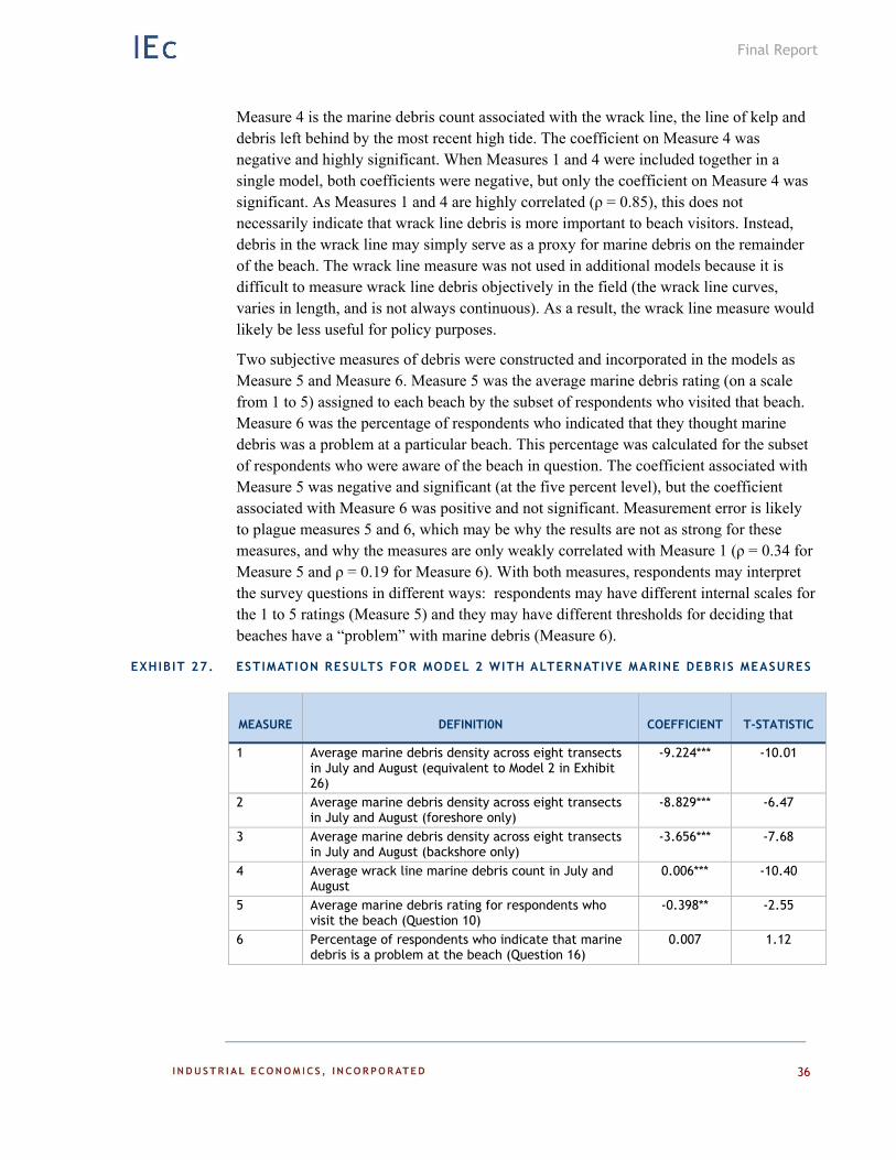
The marine debris measure used in the above models (DEBRIS) is simply the average marine debris count (items per square meter) across the eight transects completed at each beach. This measure was included in the above models primarily because it is broadly consistent with NOAA’s current protocols for marine debris measurements, which greatly facilitates benefit transfer and policy analysis. However, the mechanism by which marine debris influences beach choices is not well known, and it is certainly possible that alternative measures of marine debris are more closely linked to site choices.

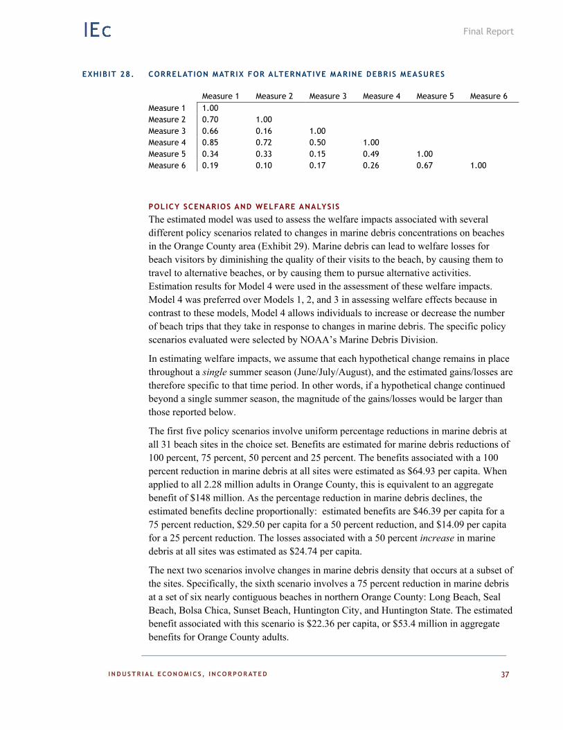
This issue was explored by estimating multiple versions of Model 2, each with a different measure of marine debris, but with identical sets of covariates. The estimation results for six different marine debris variables are presented in Exhibit 27, and the correlation matrix for the six measures is presented in Exhibit 28. Measure 1 is the baseline marine debris measure, equivalent to the measure reported in Exhibit 26. The next two measures isolate marine debris density on either the foreshore (Measure 2) or the backshore (Measure 3). The foreshore is the section of the beach below the berm that slopes down to

Final Report

35

the water. This is the area where the waves wash up on the sand. The backshore is the flat area beyond the berm where visitors lay out towels and chairs. It is not clear a priori which of the two areas would be more important to beach visitors with regard to marine debris. The results indicate that the marine debris variable is negative and highly significant with both Measure 2 (foreshore) and Measure 3 (backshore), but the coefficients are both smaller in absolute value than the coefficient associated with Measure 1.16

EXHIBIT 26. ESTIMATION RESULTS

MODEL 1 MODEL 2 MODEL 3 MODEL 4

VARIABLE

COEF. T-STAT COEF. T-STAT COEF. T-STAT COEF. T-STAT

SITE CHOICE VARIABLES

TCOST -0.122*** -20.16 -0.140*** -13.94 ‐0.131***  ‐12.79  ‐0.031***  ‐2.70 

DEBRIS -5.86*** -8.24 -9.224*** -10.01 ‐9.884***  ‐7.43  ‐2.021***  ‐2.68 

LENGTH 0.0822** 2.09 0.046  1.31  0.017*  1.84 

WIDTH -0.002 -1.61 ‐0.008***  ‐4.45  0.000  ‐1.54 

CONCESSIONS 0.990*** 5.16 0.886***  4.08  0.217***  2.75 

PIER 0.505*** 4.76 0.311***  2.63  0.106**  2.11 

FIREPITS 0.629*** 4.90 0.452***  3.72  0.139***  2.56 

COBBLES -0.495*** -2.84 ‐0.120  ‐0.61  ‐0.101**  ‐1.96 

URBAN 0.095 0.80 0.206  1.63  0.018  0.64 

WATERQ 0.057** 2.06 0.016  0.56  0.012*  1.74 

CROWDING 0.021***  4.08     

INDUSTRY 0.557***  2.94     

PARTICIPATION VARIABLES 

COLLEGE -0.202 -1.40 ASIAN 1.022*** 3.69 HISPANIC 0.737*** 3.16 ANYKIDS -0.195 -0.93 MALE -0.278* -1.74 AGE20S -0.034 -0.13 AGE30S 0.427 1.41 AGE40S 0.177 0.98 AGE60S 0.140 0.54 AGE70S 0.725*** 3.18 CONSTANT 3.823*** 5.59 Dissimilarity Coefficient

0.213*** 2.92

16 When Measures 2 and 3 were included together in a single model, both coefficients were negative and statistically significant, but the coefficient associated with Measure 2 (foreshore) was

larger (in absolute value terms) than the coefficient associated with Measure 3 (backshore). The sum of the two coefficients was approximately equal to negative nine, the coefficient

associated with Measure 1, which supports the idea that the impact of marine debris can be captured by using a measure that combines the foreshore and backshore counts.

Final Report

36

Measure 4 is the marine debris count associated with the wrack line, the line of kelp and debris left behind by the most recent high tide. The coefficient on Measure 4 was negative and highly significant. When Measures 1 and 4 were included together in a single model, both coefficients were negative, but only the coefficient on Measure 4 was significant. As Measures 1 and 4 are highly correlated (ρ = 0.85), this does not necessarily indicate that wrack line debris is more important to beach visitors. Instead, debris in the wrack line may simply serve as a proxy for marine debris on the remainder of the beach. The wrack line measure was not used in additional models because it is difficult to measure wrack line debris objectively in the field (the wrack line curves, varies in length, and is not always continuous). As a result, the wrack line measure would likely be less useful for policy purposes.

Two subjective measures of debris were constructed and incorporated in the models as Measure 5 and Measure 6. Measure 5 was the average marine debris rating (on a scale from 1 to 5) assigned to each beach by the subset of respondents who visited that beach. Measure 6 was the percentage of respondents who indicated that they thought marine debris was a problem at a particular beach. This percentage was calculated for the subset of respondents who were aware of the beach in question. The coefficient associated with Measure 5 was negative and significant (at the five percent level), but the coefficient associated with Measure 6 was positive and not significant. Measurement error is likely to plague measures 5 and 6, which may be why the results are not as strong for these measures, and why the measures are only weakly correlated with Measure 1 (ρ = 0.34 for Measure 5 and ρ = 0.19 for Measure 6). With both measures, respondents may interpret the survey questions in different ways: respondents may have different internal scales for the 1 to 5 ratings (Measure 5) and they may have different thresholds for deciding that beaches have a “problem” with marine debris (Measure 6).

EXHIBIT 27. ESTIMATION RESULTS FOR MODEL 2 WITH ALTERNATIVE MARINE DEBRIS MEASURES

MEASURE DEFINITI0N COEFFICIENT T-STATISTIC

1 Average marine debris density across eight transects in July and August (equivalent to Model 2 in Exhibit 26)

-9.224*** -10.01

2 Average marine debris density across eight transects in July and August (foreshore only)

-8.829*** -6.47

3 Average marine debris density across eight transects in July and August (backshore only)

-3.656*** -7.68

4 Average wrack line marine debris count in July and August

0.006*** -10.40

5 Average marine debris rating for respondents who visit the beach (Question 10)

-0.398** -2.55

6 Percentage of respondents who indicate that marine debris is a problem at the beach (Question 16)

0.007 1.12

Final Report

37

EXHIBIT 28. CORRELATION MATRIX FOR ALTERNATIVE MARINE DEBRIS MEASURES

Measure 1 Measure 2 Measure 3 Measure 4 Measure 5 Measure 6 Measure 1 1.00 Measure 2 0.70 1.00 Measure 3 0.66 0.16 1.00 Measure 4 0.85 0.72 0.50 1.00 Measure 5 0.34 0.33 0.15 0.49 1.00 Measure 6 0.19 0.10 0.17 0.26 0.67 1.00

POLICY SCENARIOS AND WELFARE ANALYSIS

The estimated model was used to assess the welfare impacts associated with several different policy scenarios related to changes in marine debris concentrations on beaches in the Orange County area (Exhibit 29). Marine debris can lead to welfare losses for beach visitors by diminishing the quality of their visits to the beach, by causing them to travel to alternative beaches, or by causing them to pursue alternative activities. Estimation results for Model 4 were used in the assessment of these welfare impacts. Model 4 was preferred over Models 1, 2, and 3 in assessing welfare effects because in contrast to these models, Model 4 allows individuals to increase or decrease the number of beach trips that they take in response to changes in marine debris. The specific policy scenarios evaluated were selected by NOAA’s Marine Debris Division.

In estimating welfare impacts, we assume that each hypothetical change remains in place throughout a single summer season (June/July/August), and the estimated gains/losses are therefore specific to that time period. In other words, if a hypothetical change continued beyond a single summer season, the magnitude of the gains/losses would be larger than those reported below.

The first five policy scenarios involve uniform percentage reductions in marine debris at all 31 beach sites in the choice set. Benefits are estimated for marine debris reductions of 100 percent, 75 percent, 50 percent and 25 percent. The benefits associated with a 100 percent reduction in marine debris at all sites were estimated as $64.93 per capita. When applied to all 2.28 million adults in Orange County, this is equivalent to an aggregate benefit of $148 million. As the percentage reduction in marine debris declines, the estimated benefits decline proportionally: estimated benefits are $46.39 per capita for a 75 percent reduction, $29.50 per capita for a 50 percent reduction, and $14.09 per capita for a 25 percent reduction. The losses associated with a 50 percent increase in marine debris at all sites was estimated as $24.74 per capita.

The next two scenarios involve changes in marine debris density that occurs at a subset of the sites. Specifically, the sixth scenario involves a 75 percent reduction in marine debris at a set of six nearly contiguous beaches in northern Orange County: Long Beach, Seal Beach, Bolsa Chica, Sunset Beach, Huntington City, and Huntington State. The estimated benefit associated with this scenario is $22.36 per capita, or $53.4 million in aggregate benefits for Orange County adults.

Final Report

38

The seventh scenario involves a 100 percent reduction in marine debris at the five sites that currently have the highest marine debris densities: Dockweiler (0.21 items/m2), Long Beach (0.18 items/m2), Redondo Beach (0.16 items/m2), Corona Del Mar (0.14 items/m2), and Balboa (0.13 items/m2). The estimated benefit associated with this scenario is $27.60 per capita, or $63.1 million in aggregate benefits for Orange County adults.

The final scenario assesses the benefits associated with the removal of all parking fees at the 31 beach sites. This scenario assumes that the removal of these fees would not cause congestion problems due to increased use of beach parking lots. It also assumes that under current conditions, the fees themselves generate no benefits to Orange County residents. That is, it assumes that removing these fees would not lead to any reductions in services or deferred maintenance of beach facilities. Although these assumptions are somewhat unrealistic, this scenario is nonetheless useful for comparison purposes. The estimated benefit associated with this scenario is $161.57 per capita, or $369 million in aggregate benefits for Orange County adults. With an estimated 26.4 million beach trips taken by Orange County residents under current conditions, this is equivalent to approximately $14 in benefits for every beach trip, which is similar to the typical cost of parking for the day at an Orange County beach.

PER TRIP VALUES

In addition to standard aggregate estimates of welfare losses/gains, per trip values are often useful within the context of benefit transfer efforts. As these transfers are implemented in a variety of contexts, two different types of per trip values are provided here. First, for each policy scenario, we divide the estimated aggregate gain/loss by the total predicted trips to the impacted sites under baseline conditions (i.e., prior to implementing the policy). The resulting values range from -$2.14 per trip for a 50% increase in marine debris at all sites to $18.84 per trip for eliminating all marine debris at the five worst sites (Exhibit 29).

Second, the ratio of any coefficient from the site choice model to the travel cost coefficient can be interpreted as the per-trip benefit associated with a one-unit change in the selected coefficient – assuming that both the total number of trips and the allocation of those trips across sites are held constant. For example, by dividing the coefficient on DEBRIS in model 4 (2.021) by the coefficient on TCOST (0.031), we obtain $65.19. This can be interpreted as the per-trip benefit to visitors at a given beach of a one-unit decline in DEBRIS at that beach. However, with the current set of sites, a one-unit decline in DEBRIS is not feasible, as the beach with the largest amount of debris (Dockweiler) only has 0.21 items/m2. Alternatively, consider a 25% reduction in marine debris at a site with average debris density (0.08 items/m2), or a reduction of 0.02 items/m2. The per trip benefit associated with this 25% reduction is equal to 0.02 x $65.19, or $1.30 per trip. This approach can provide a per trip value that aligns more closely with the specific change that will occur at the policy site, but it relies on the assumption that beach visitors will not substitute to the improved site.

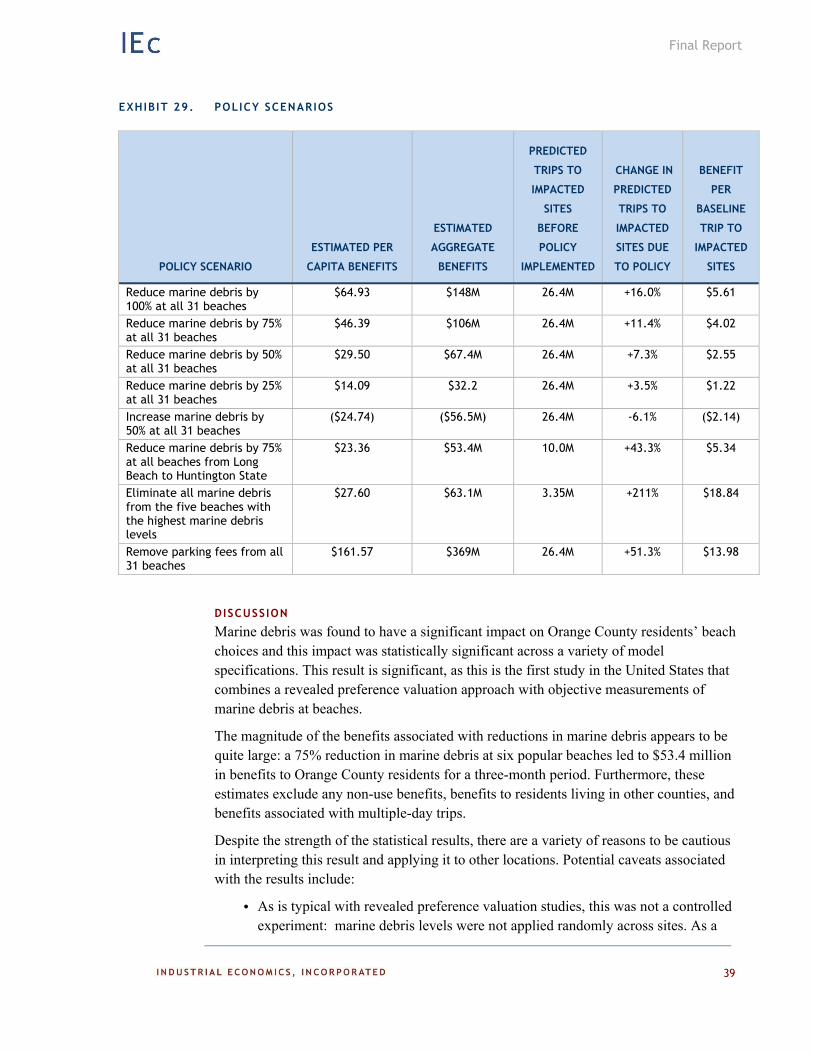
Final Report

39

EXHIBIT 29. POLICY SCENARIOS

POLICY SCENARIO

ESTIMATED PER

CAPITA BENEFITS

ESTIMATED

AGGREGATE

BENEFITS

PREDICTED

TRIPS TO

IMPACTED

SITES

BEFORE

POLICY

IMPLEMENTED

CHANGE IN

PREDICTED

TRIPS TO

IMPACTED

SITES DUE

TO POLICY

BENEFIT

PER

BASELINE

TRIP TO

IMPACTED

SITES

Reduce marine debris by 100% at all 31 beaches

$64.93 $148M 26.4M +16.0% $5.61

Reduce marine debris by 75% at all 31 beaches

$46.39 $106M 26.4M +11.4% $4.02

Reduce marine debris by 50% at all 31 beaches

$29.50 $67.4M 26.4M +7.3% $2.55

Reduce marine debris by 25% at all 31 beaches

$14.09 $32.2 26.4M +3.5% $1.22

Increase marine debris by 50% at all 31 beaches

($24.74) ($56.5M) 26.4M -6.1% ($2.14)

Reduce marine debris by 75% at all beaches from Long Beach to Huntington State

$23.36 $53.4M 10.0M +43.3% $5.34

Eliminate all marine debris from the five beaches with the highest marine debris levels

$27.60 $63.1M 3.35M +211% $18.84

Remove parking fees from all 31 beaches

$161.57 $369M 26.4M +51.3% $13.98

DISCUSSION

Marine debris was found to have a significant impact on Orange County residents’ beach choices and this impact was statistically significant across a variety of model specifications. This result is significant, as this is the first study in the United States that combines a revealed preference valuation approach with objective measurements of marine debris at beaches.

The magnitude of the benefits associated with reductions in marine debris appears to be quite large: a 75% reduction in marine debris at six popular beaches led to $53.4 million in benefits to Orange County residents for a three-month period. Furthermore, these estimates exclude any non-use benefits, benefits to residents living in other counties, and benefits associated with multiple-day trips.

Despite the strength of the statistical results, there are a variety of reasons to be cautious in interpreting this result and applying it to other locations. Potential caveats associated with the results include:

As is typical with revealed preference valuation studies, this was not a controlled experiment: marine debris levels were not applied randomly across sites. As a

Final Report

40

result, it is impossible to completely rule out the possibility of omitted variables bias. Suppose, for example, that municipalities in the area dedicate more resources to controlling and removing marine debris at sites that are already popular with visitors for other reasons. If these other factors are not included in our model, then the parameter estimate associated with marine debris may be biased.

The survey was implemented in November/December, but it collected data on beach trips taken several months earlier – in June, July, and August. This gap may lead to recall errors, and the extent to which recall errors affects trip reporting in the current dataset is unknown.

Marine debris levels may vary throughout the day due to natural processes (winds, waves, currents), visitors leaving garbage on the sand, and beach raking activities. Ideally, debris measurements would be made during the peak time period for beach visitation so the measurements reflect debris concentrations that the majority of visitors observe during a trip. However, during the peak period, it is also extremely difficult to lay out transects for beach counts in randomly selected locations without disturbing visitors. As a result, measurements were generally made in the morning before beaches became too crowded.

For approximately 18 percent of the beach trips, the precise destination is uncertain due to respondents’ vague site descriptions. Specifically, some respondents listed “Huntington” as the destination and did not distinguish between Huntington State and Huntington City. Similarly, some respondents listed “Laguna” as the destination rather than “Laguna Coves” or “Laguna Main.” These trips with ambiguous destinations where allocated randomly to the more specific sites, with probabilities proportional to the percentage of trips to each site.

An examination of trip patterns appears to indicate that respondents occasionally went for long walks, runs, or bike rides and visited several beaches during a single day trip. In retrospect, the survey instrument did not provide clear instructions for these situations, and it appears that a subset of respondents may have recorded each of these more than once. If this occurred, then travel costs would be overstated because round-trip travel costs would effectively be assigned to every destination visited during a single day trip. No adequate solution to this issue could be identified, as the data do not allow us to unambiguously identify such trips. As a partial solution for avid visitors, visits were scaled down (proportionally) to an average of two trips per day for respondents who reported more than two trips per day in any given month.

TRANSFERABILITY OF RESULTS

The current study was designed as a pilot, with the primary goals being to (1) assess benefits to Orange County residents of reductions in marine debris and (2) assess the usefulness of a specific technique for estimating benefits associated with marine debris removal. As the survey was mailed to a simple random sample of all Orange County residential addresses, the benefit estimates can be extrapolated to the adult population of

Final Report

41

Orange County with confidence, allowing for caveats related to potential non-response bias.

Transferring these estimated benefits outside of the summer period and outside of Orange County requires careful assessment of potential differences between the study site and alternative site should be completed. Potential issues that should be evaluated include:

Baseline Marine Debris Levels. For example, if Orange County beaches are generally cleaner than the alternative site, then a 50 percent reduction in debris may provide greater value at the alternative site: the reduction may bring the debris levels below a threshold level of acceptability for beach visitors.

Types of Marine Debris. For example, if large debris items on Orange County beaches are primarily plastic, but an alternative site is plagued by metal cans and glass, the benefits associated with reductions in the total debris counts may not be similar.

Residents’ Sensitivity to Marine Debris. In some cultures and in some areas of the country, it may be considered more acceptable to have marine debris on the beach. If that is the case, then the benefits associated with removing debris in these locations may be lower than in Orange County.

Available Substitutes. The benefits associated with reductions in marine debris will be greater in locations where there are fewer high quality substitutes for recreating at beaches plagued by high concentrations of marine debris. For example, if nearby alternative beaches are scarce or if there are no alternative swimming options (e.g., community swimming pools), then the benefits of reductions in marine debris will be greater.

Climate. As beach visitation is higher during warmer months, reductions in marine debris will provide lower per capita benefits in climates where beach visitation is rare in the winter (i.e., in New England).

Given the similarity of the available substitutes, the benefits to Orange County residents could potentially be applied to estimate benefits to residents of Los Angeles County. The most appropriate approach to implementing this transfer would be through a benefit function approach (possibly at the zip code level), which would allow one to account for the spatial distribution of the population as well as demographic differences between the two counties. In addition, it may be reasonable to transfer benefits (on a per trip basis) to non-summer months within Orange and Los Angeles Counties. Transfers beyond the Orange County/Los Angeles area would require careful consideration of the above issues.

RECOMMENDATIONS FOR FUTURE RESEARCH

The current study was designed as a pilot effort to explore the feasibility of applying a revealed preference valuation approach to estimate the benefits associated with reductions in marine debris. However, the study was useful not only in achieving the relatively narrowly-defined goal of estimating benefits to Orange County residents, but also in

Final Report

42

providing insights for future research efforts related to marine debris valuation. This section describes recommendations related to future research.

1. Selection of Alternative Site for Application of Current Methodology: The current effort provided estimates of the benefits of reductions in marine debris to Orange County residents. However, similar reductions in other locations may not provide similar benefits for a variety of reasons, including those mentioned above. As a result it would likely be informative to apply a similar approach to alternative locations to assess the robustness of the results. The following issues should be considered in selecting an alternative study location:

The available beaches must vary with respect to the amount of marine debris that is observable to visitors. The model makes inferences about willingness-to-pay for reductions in marine debris by observing choices among beaches that differ in the amount of debris and in the cost of traveling to the beach. Without variation in marine debris across beaches, visitors’ beach choices would not provide any information about the benefits of debris removal.17

There must be a sufficient number of beaches in the local area. If there are a limited number of beaches available to local residents, then it may be difficult to isolate the impact of marine debris (separate from the impact of other beach characteristics). For example, if only one beach in the area has significant marine debris problems, then it would be difficult to determine whether visitors are avoiding that beach because of marine debris or because of other characteristics uniquely associated with that location (e.g., it may be the only beach in the local area without restrooms or without adequate parking). Ideally, there would be at least ten beaches from which local residents could choose for a day trip.

The beaches must be well defined and easily identified by visitors. The valuation approach relies on visitors’ ability to describe which beach was visited, so that trip data can be linked with data on marine debris for specific locations. As a result, the local beaches must have well-known names or other distinguishing characteristics that would allow survey respondents to provide information about specific destinations that were visited. Locations with long, uninterrupted expanses of shoreline with nearly continuous access opportunities (e.g., the Outer Banks of North Carolina) would likely be difficult to study, as survey respondents may not be able to identify specific beaches that were visited.

The beaches must be visited frequently by residents of the local area. The methodology requires data on beach trips, so it is important that the beaches be

17 Note that this is not equivalent to saying that there would be no benefits associated with marine debris removal at these locations: there may be benefits, but they cannot be measured using

revealed preference valuation techniques.

Final Report

43

relatively popular with local residents, thus increasing the likelihood of encountering beach visitors through a general population survey. In Alaska, for example, there may be well defined beaches with varying levels of marine debris, but the climate is unlikely to be conducive to a large number of beach visits by local residents.

2. Modifications to Current Valuation Methodology: If the current valuation approach is replicated at an alternative location, we would recommend a number of changes based on the experience gained through the current study:

The recall period for beach trips should be reduced to one or two months in order to minimize recall error and the potential for telescoping bias. While we have no evidence that recall issues plagued the current study, we also cannot rule out recall problems, and they seem likely to have arisen for the high-frequency beach visitors in the dataset (e.g., respondents who took more than 100 trips).

While the planned recall period was three months in the current study, it expanded due to requirements the Paperwork Reduction Act (PRA) approval process. In future efforts, we recommend that the PRA process be completed prior to the collection of any marine debris data.

With a recall period of one or two months, multiple survey waves would likely be necessary to cover the primary beach visitation months. We recommend drawing independent samples of the population for each wave, as repeat-contact surveys are plagued by attrition, thus complicating modeling efforts.

The current study used a mail survey mode (rather than telephone or in-person). We believe the mail survey implementation was generally successful and offers the best combination of a reasonable response rate and low cost. However, one disadvantage of a mail survey is the inability to ask follow-up questions that clarify unusual responses. In particular, we suspect that a subset of the beach “trips” that were recorded in the current effort may not have been separate trips from the respondent’s home (with additional round-trip travel costs incurred) but instead were simply extensions of another trip that had already been recorded. For example, rather than taking a trip to Balboa Beach and a trip to Newport Beach, the respondent may have simply walked along the beach and therefore visited both sites during a single trip from home. A follow-up study should clarify the questionnaire language in order to clearly identify such trips.

The non-respondent follow-up survey identified preliminary evidence of avidity bias, with frequent beach visitors potentially being over-represented among the respondents to the main survey. However, despite sending surveys via FedEx and despite having an extremely short (five-question) questionnaire, the response rate for the non-respondent follow-up survey was low, leading to a final sample size that was not adequate for use in reweighting data from the

Final Report

44

main survey. Furthermore, although survey weights were developed that adjusted for differences in responses rates across geographic areas and calibrated the survey data to match census demographics for Orange County, we cannot be certain that these weights adequately addressed avidity bias. In future work, we recommend addressing this issue by either: (1) considerably increasing the resources devoted to the non-response follow-up study (e.g., multiple contacts, contacts via multiple modes, etc.) or (2) presenting upper and lower bound benefit estimates, where the upper bound assumes that non-respondents are identical to respondents and the lower bound assumes that non-respondents have zero benefits.

One option for increasing the response rate would be to include a postcard with each mailing that allows non-beach visitors to opt out of the study by checking a box that says something like “Please do not send me additional survey materials because I never visit local beaches.” These individuals would then be classified as ineligible when calculating the overall response rate, and the population size for aggregating benefits would be reduced by the percentage of sampled individuals who were deemed ineligible.

One alternative to the current method that would allow for additional flexibility in exploring perceptions of debris would be to implement an on-site choice experiment study, with debris levels illustrated for the respondent using “test plots” in the sand near the back of the beach. Visitors would be intercepted as they are leaving the beach, and they would be asked to complete a short questionnaire that would include a series of hypothetical beach choices. The characteristics of the hypothetical beaches would vary by design, and one of those characteristics would be level of marine debris. The respondent would be asked to refer to side-by side test plots in the sand that depict varying levels of debris associated with the hypothetical beaches in the choice questions. The debris could be collected at the site so that it mimics the type of debris that one would expect visitors to observe. The primary advantage of this approach is that it allows the researcher to experimentally change the quantity and type of debris, which is generally not possible with revealed preference studies. This would allow for a more nuanced assessment of the impact of marine debris on behavior. The response rate is also likely to be fairly high with an on-site intercept survey. The primary disadvantage of this approach is that it does not rely on actual behavior. In addition, aggregating any benefits to the population of users would be more complicated due to on-site sampling.

Final Report

45

REFERENCES

Haab, T.C. and K.E. McConnell. (2002). Valuing Environmental and Natural Resources: The Econometrics of Non-Market Valuation. Cheltenham, UK: Edward Elgar.

Hanemann, W.M. (1982). “Applied Welfare Analysis with Qualitative Response Models”. Working Paper No. 241, Giannini Foundation of Agricultural Economics, University of California: Berkeley.

Heal the Bay. (2013). “Heal the Bay’s 2012-2013 Annual Beach Report Card. Santa Monica, California. http://www.healthebay.org/sites/default/files/pdf/BRC_2014_WEB.pdf

International Hydrographic Organization (IHO). (1999). S-32 – Hydrographic Dictionary, Fifth Edition. Special Publication No. 32: Part 1, Vol. 1. 1994. Jones, C.A. and F. Lupi. “The Effect of Modeling Substitute Activities on Recreational Benefit Estimates.” Marine Resource Economics 14(4): 357-374.

Kalton, G. (1983). “Compensating for Missing Survey Data”. Survey Research Center, Institute for Social Research, University of Michigan.

Kling, C. L., Thomson, C.J. (1996). “The Implications of Model Specification for Welfare Estimation in Nested Logit Models”. American Journal of Agricultural Economics 78: 103-114.

Moore, S.L., D. Gregorio, M. Carreon, S.B. Weisberg, and M.K. Leecaster. “Composition and Distribution of Beach Debris in Orange County, California” Marine Pollution Bulletin, 42(3): 241-245. 2001.

Opfer, S., C. Arthur, and S. Lippiatt. NOAA Marine Debris Shoreline Survey Field Guide. January 2012.

U.S. DOC. (2013). National Oceanic and Atmospheric Administration, Tides and Currents. NOAA Tide Predictions- California. (http://tidesandcurrents.noaa.gov/tide_predictions.html?gid=235).

U.S. Census Bureau. (2013). 2013 TIGER/Line Shapefiles. (http://www.census.gov/cgi-bin/geo/shapefiles2013/main).

U.S. Census Bureau. (2013). State and County QuickFacts. Updated May 23, 2013 (http://quickfacts.census.gov/qfd/index.html).