Assessing Risks to Biodiversity from Future Landscape Change : Evaluación de Riesgos para la Biodiversidad Debido a Cambios Futuros en el Paisaje

349

Conservation Biology, Pages 349–360Volume 11, No. 2, April 1997

Contributed Papers

Assessing Risks to Biodiversity fromFuture Landscape Change

DENIS WHITE,* PRISCILLA G. MINOTTI,* MARY J. BARCZAK,* JEAN C. SIFNEOS,* KATHRYN E. FREEMARK,† MARY V. SANTELMANN,* CARL F. STEINITZ,‡A. ROSS KIESTER,§ AND ERIC M. PRESTON**

*Department of Geosciences, Oregon State University, Corvallis, OR 97331, U.S.A.†Environment Canada, c/o US EPA, 200 SW 35th St., Corvallis, OR 97333, U.S.A.‡Graduate School of Design, Harvard University, 48 Quincy St., Cambridge, MA 02138, U.S.A.§USDA Forest Service, 3200 SW Jefferson Way, Corvallis, OR 97331, U.S.A.**US Environmental Protection Agency, 200 SW 35th St., Corvallis, OR 97333, U.S.A.

Abstract:

We examined the impacts of possible future land development patterns on the biodiversity of alandscape. Our landscape data included a remote sensing derived map of the current habitat of the studyarea and six maps of future habitat distributions resulting from different land development scenarios. Ourspecies data included lists of all bird, mammal, reptile, and amphibian species in the study area, their habitatassociations, and area requirements for each. We estimated the area requirements using home ranges, sam-pled population densities, or genetic area requirements that incorporate dispersal distances. Our measures ofbiodiversity were species richness and habitat abundance. We calculated habitat abundance in two ways.First, we computed the total habitat area for each species in each landscape. Second, we calculated the num-ber of habitat units for each species in each landscape by dividing the size of each habitat patch in the land-scape by the area requirement and summing over all patches. Species richness was based on presence of hab-itat. Species became extinct in the landscape if they had no habitat area or no habitat units, respectively. Wethen computed ratios of habitat abundance in each future landscape to habitat abundance in the present foreach species. We also computed the ratio of future to present species richness. We then calculated summarystatistics across all species. Species richness changed little from present to future. There were distinctly greaterrisks to habitat abundance in landscapes that extrapolated from present trends or zoning patterns, however,as opposed to landscapes in which land development activities followed more constrained patterns. These re-sults were stable when tested using Monte Carlo simulations and sensitivity tests on the area requirements.We conclude that this methodology can begin to discriminate the effects of potential changes in land develop-ment on vertebrate biodiversity.

Evaluación de Riesgos para la Biodiversidad Debido a Cambios Futuros en el Paisaje

Resumen:

Examinamos los impactos en la biodiversidad de un paisaje debidos a posibles patrones de modi-ficación del suelo. Nuestros datos de paisage incluyen un mapa del área de estudio actual derivado de sen-sores remotos y seis mapas de distribuciones futuras del hábitat que resultan de diferentes escenarios de de-sarrollo del suelo. Nuestros datos de especies incluyen listas de todas las especies de aves, mamíferos, reptiles yanfibios del área de estudio, sus asociaciones de hábitat y los requeriminteos de espacio para cada una de el-las. Estimamos los requerimientos de área usando rangos de hogar, densidades de poblaciones muestreadaso requerimientos genéticos de área que incorporan destancias de dispersión. Las medidas de biodiversidadfueron la riqueza de especies y la abundancia del hábitat. La abundancia del hábitat fue estimada en dosformas. Primero, estimamos el área total del hábitat para cada especie en cada paisaje. Segundo, calculamosel número de unidades de hábitat para cada especie en cada paisaje dividiendo el tamaño de cada parche dehabitat en el paisaje por el requerimiento de área y sumando para todos los parches. La riqueza de especies

Address correspondence to Denis White, email whitede@ ucs.orst.eduPaper submitted November 1, 1995; revised manuscript accepted June 19, 1996.

350

Landscape Changes and Biodiversity White et al.

Conservation BiologyVolume 11, No. 2, April 1997

se basó en la presencia de hábitat. La extinción de especies en un paisaje ocurrió cuando la especie no teníaárea de hábitat o unidades de hábitat respectivamente. Posteriormente estimamos la proporción entre laabundancia del hábitat en cada paisaje futuro y la abundancia de hábitat en el presente para cada especie.Tambien estimamos la proporción entre riqueza de especies futura y presente. Se desarrolló un resumen es-tadístico para todas las especies. La riqueza de las especies cambió poco del presente al futuro. De cualquiermanera, existieron grandes riesgos distintivos para la abundancia de hábitat en paisajes que fueron extrapo-lados a partir de tendencias actuales o patrones de zonificación opuestos a paisajes en los cuales las activi-dades de desarrollo siguieron patrones restringidos. Estos resultados fueron estables al ser evaluados usandosimulaciones Monte Carlo y pruebas de sensitividad para requerimientos de áreas. Concluímos que estametodología puede iniciar la descriminación de efectos en la biodiversidad de vertebrados debido a cambios

potenciales en el desarrollo del suelo.

Introduction

Land-use practices are a major cause of the decline inbiodiversity in recent decades (Soulé 1991). Conserva-tion efforts have focused on maintaining biological di-versity primarily by minimizing exposure to human ac-tivities through establishment of networks of protectedareas. Gap Analysis (Scott et al. 1987, 1993) is a compre-hensive approach to assessing conservation needs overlarge geographic regions. This approach has pioneeredthe use of vegetation maps, species-habitat associations,and geographic ranges of species to model the predicteddistribution of native terrestrial vertebrate species in or-der to identify “gaps” in biodiversity protection. By over-laying maps of currently protected areas, Gap Analysisdetermines the number of species currently not pro-tected. The long-term conservation of biological diver-sity is dependent not only on establishment of protectedareas, however, but also on maintaining hospitable envi-ronments and viable populations within managed land-scapes (Noss & Harris 1986; Western 1989; Hansen et al.1991; Shafer 1994).

Impacts of habitat loss and fragmentation associatedwith some land-use practices, for example, agriculture,have been well studied for some species, particularlybirds, in remnants of native vegetation (e.g., forests,marshes, prairies) (Freemark 1995; Martin & Finch 1995).Only a few recent studies, however, have attempted tosystematically and quantitatively assess risks to biodiver-sity at the landscape scale. Best et al. (1995) used spe-cies-habitat associations to assess the impact of differentagricultural landscapes on numbers of bird species po-tentially nesting in Iowa farmland. Hansen et al. (1993)developed an approach to identify bird species at risk inforests in western Oregon and Washington at presentand under four disturbance-management scenarios overa 140-year period. They used habitat maps, species-habi-tat associations, and other natural history characteristicsof species to quantify habitat suitability for each birdspecies. For present conditions species at risk were in-ferred from shortages of suitable habitat. Risks posed byalternative futures were inferred from patterns of habitatdiversity and richness.

Methods are needed for predicting potential impactsof human activities on biological diversity across a hier-archy of spatial and temporal scales to make land useplanning both clearer and better informed (Hansen et al.1993; Dale et al. 1994; Freemark 1995). We present anapproach for estimating potential risk to biodiversityfrom future landscape change associated with land de-velopment. The essential components of the approachare (1) a large, representative sample or enumeration ofspecies; (2) natural history characteristics of the species,specifically their habitat and area requirements; (3) amap of habitats; (4) future landscape alternatives thatcan be mapped as changes in habitat; and (5) a methodto assess potential risk posed by future landscapes com-pared to the present using summary statistics of changesin species richness and habitat abundance.

Geographical Setting

This study was conducted in Monroe County, Pennsylva-nia, which is approximately 1580 km

2

in area and lies inthe northeastern part of the state (Fig. 1), forming thecore of the Poconos region. This region is defined physi-

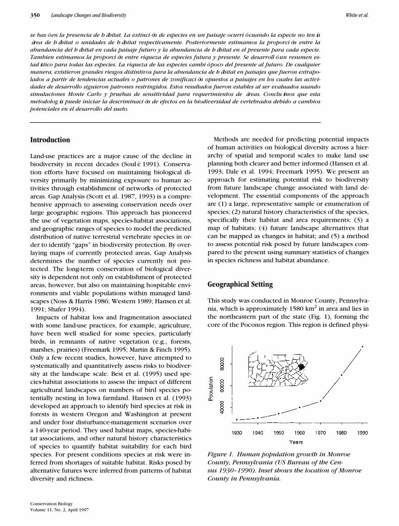
Figure 1. Human population growth in Monroe County, Pennsylvania (US Bureau of the Cen-sus 1930–1990). Inset shows the location of Monroe County in Pennsylvania.


White et al. Landscape Changes and Biodiversity

351

cally by the Pocono Plateau, an uplifted sedimentary ba-sin about 600 m in mean elevation at the southern edgeof the Wisconsin glaciation. The plateau covers about40% of the county and is characterized by lakes and for-ests. In addition to the plateau, the county has two otherregions. The region to the east of the plateau is part ofthe Allegheny uplands, an area similar to the plateau butwith a mean elevation of about 300 m. The southern40% of the county is part of the ridge and valley regionof Pennsylvania. The natural history of the Poconos re-gion is described in Oplinger and Halma (1988) and itssignificance for conservation in Smith and Richmond(1994). Monroe County is divided politically into 20 mu-nicipalities comprised of 16 townships and four bor-oughs. The boroughs are smaller areal units with higherdensities of human population. Most land-use decisionsare made at the level of the municipalities.

The Poconos region has been a prominent recreationand vacation area since the nineteenth century for peo-ple from large metropolitan areas that are within severalhours travel time by train or automobile. With the intro-duction of the interstate highway system in the 1960sand 1970s the number of permanent residents has in-creased along with recreational use. The populationtrend for the county shows a noticeable inflection up-ward at the census of 1970 (Fig. 1). This region repre-sents a classic situation of potential loss of natural habi-tat due to increased human activities.

Habitat Map and Future Alternatives

Smith and Richmond (1994) prepared a habitat map forthe county in conjunction with the Cornell Laboratoryfor Environmental Applications of Remote Sensing(CLEARS). The source material for the map is a portionof a single Landsat Thematic Mapper scene from 21 June1991 covering all of Monroe County. The CLEARS regis-tered and classified the TM scene according to standardsof the GAP program (Scott et al. 1993); the spatial reso-lution was 25 m. The final classification contained 13habitat classes (Table 1).

Six possible alternative versions of the landscape andhabitats of Monroe County in the year 2020 were pre-pared by Steinitz et al. (1994). These came from a studythat had the objectives of describing the patterns andsignificant human and natural processes affecting thelandscape of the county, constructing geographic infor-mation system models to simulate these processes andpatterns, creating changes in the landscape by forecast-ing and by design, and evaluating how the changes af-fect pattern and process using the models. The studyidentified six kinds of issues in the future developmentof the landscape of the county: geological, biological, vi-sual, demographic, economic, and political. These issues

became the basis for evaluating the existing conditionsof the county and developing alternative futures.

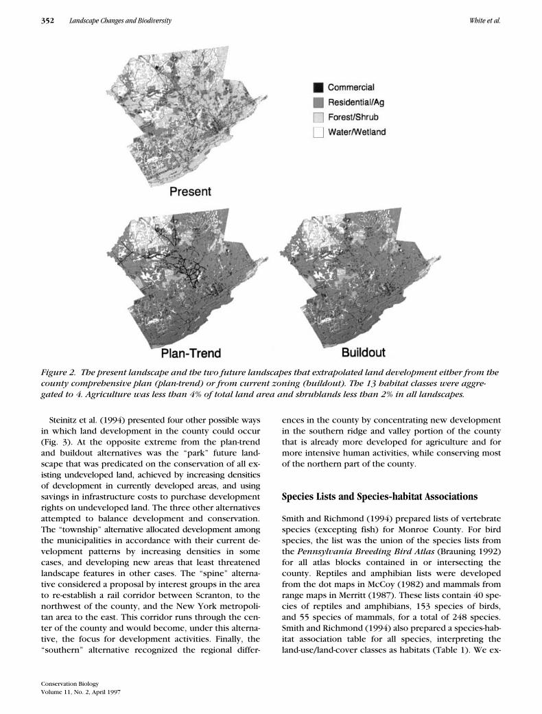
The alternative future landscapes were based on a mod-ified version of the Smith and Richmond land-use/land-cover map. Steinitz et al. represented low density residen-tial development more accurately than on the Smith andRichmond map by using digital road data and othersources. They represented wetland areas more accuratelythan on the Smith and Richmond map by using NationalWetlands Inventory maps. With these changes they createda more accurate map of existing conditions in the county.We used this map as the baseline for our biodiversityanalysis and called it the “present” landscape (Fig. 2).

The future landscapes described by Steinitz et al. (1994)differed both in degree and spatial distribution of humanimpact. These landscape alternatives all assumed a dou-bling of the human population by the year 2020, a pro-jection based on the current rate of growth (Fig. 1). Thefuture alternatives represented different ways in whichthis population increase might be accommodated. TheMonroe County Planning Commission staff assisted Steinitzet al. in preparing the future scenarios. Two future alter-natives were derived by extrapolating from currenttrends and zoning patterns (Fig. 2). The “plan-trend” al-ternative was based on implementation of the countycomprehensive plan of 1981 and extended the patternof land development that has occurred since that time.This pattern included deviations from the plan in somecases. The “buildout” alternative started with the cur-rent zoning plans for each municipality and assumedthat the full development allowed in each plan wouldoccur. This alternative represented an extreme level ofhuman impact where most remaining undeveloped, butdevelopable, land in Monroe County would be devel-oped. The only large patches of land not developed inthese two future landscapes were existing national park,state park, state forest, and state game lands. By the year2020 the county would then resemble suburban areas inneighboring New Jersey or near Philadelphia.

Table 1. Number of species in major groups assigned to each habitat class.*

Habitat class Herps Birds Mammals All verts

Commercial-industrial 1 9 10 20Residential 12 84 32 128Agricultural 13 82 41 136Lacustrine limnetic 14 19 4 37Lacustrine littoral 22 26 5 53Palustrine 27 28 14 69Shrublands (successional) 26 64 38 128Hemlock 20 53 40 113White Pine 22 66 42 130White Pine-hardwoods 27 95 46 168Oak-heath 28 95 44 167Sugar Maple-Red Oak 27 101 49 177Sugar Maple-Ash-Basswood 27 98 49 174

*

Smith and Richmond (1994)

352



Steinitz et al. (1994) presented four other possible waysin which land development in the county could occur(Fig. 3). At the opposite extreme from the plan-trendand buildout alternatives was the “park” future land-scape that was predicated on the conservation of all ex-isting undeveloped land, achieved by increasing densitiesof development in currently developed areas, and usingsavings in infrastructure costs to purchase developmentrights on undeveloped land. The three other alternativesattempted to balance development and conservation.The “township” alternative allocated development amongthe municipalities in accordance with their current de-velopment patterns by increasing densities in somecases, and developing new areas that least threatenedlandscape features in other cases. The “spine” alterna-tive considered a proposal by interest groups in the areato re-establish a rail corridor between Scranton, to thenorthwest of the county, and the New York metropoli-tan area to the east. This corridor runs through the cen-ter of the county and would become, under this alterna-tive, the focus for development activities. Finally, the“southern” alternative recognized the regional differ-

ences in the county by concentrating new developmentin the southern ridge and valley portion of the countythat is already more developed for agriculture and formore intensive human activities, while conserving mostof the northern part of the county.

Species Lists and Species-habitat Associations

Smith and Richmond (1994) prepared lists of vertebratespecies (excepting fish) for Monroe County. For birdspecies, the list was the union of the species lists fromthe

Pennsylvania Breeding Bird Atlas

(Brauning 1992)for all atlas blocks contained in or intersecting thecounty. Reptiles and amphibian lists were developedfrom the dot maps in McCoy (1982) and mammals fromrange maps in Merritt (1987). These lists contain 40 spe-cies of reptiles and amphibians, 153 species of birds,and 55 species of mammals, for a total of 248 species.Smith and Richmond (1994) also prepared a species-hab-itat association table for all species, interpreting theland-use/land-cover classes as habitats (Table 1). We ex-

Figure 2. The present landscape and the two future landscapes that extrapolated land development either from the county comprehensive plan (plan-trend) or from current zoning (buildout). The 13 habitat classes were aggre-gated to 4. Agriculture was less than 4% of total land area and shrublands less than 2% in all landscapes.



353

cluded from our analyses 8 species introduced by hu-mans plus 9 species for which we were unable to obtainarea requirements. Therefore we used a total of 231 spe-cies: 40 species of herpetofauna, 147 species of birds,and 44 species of mammals.

In mapping the future alternatives, Steinitz et al.(1994) used several classes of residential developmentand several classes of roads to represent their scenariosmore accurately. The total number of classes in theunion of their classifications was 35. The Smith andRichmond species-habitat association table, however,only assigned species to the 13 classes on the Smith andRichmond map. Therefore we reduced each of the Stein-itz et al maps from 35 classes to 13 by assigning all Stein-itz et al. classes to one of the Smith and Richmond classes.

Species Area Requirements

As an initial step toward incorporating a more completeapproximation of natural history and demographic char-acteristics of species, we estimated an area requirement

(Mühlenberg et al. 1991) for the species in our study.Area requirements represent an initial estimate of spacerequired for a reproductive or breeding unit of a species.Breeding units may be individuals (females), a breedingpair, or some set of individuals such as a deme or a col-ony. We defined area requirements as home ranges, ter-ritory sizes, sampled population densities, or dispersaldistances, depending on the type of reproductive unit.For each major taxonomic group we consulted appro-priate literature and adapted the area requirement con-cept accordingly. Because the reported area require-ments for many species have a range of values, we usedboth minimum and maximum values for each species;for some species these were the same. Across all speciesthe minimum values and the maximum values rangedfrom 0.002 to 19,600 ha. The median of the minimumvalues was 1.1 ha and the median of the maximum val-ues was 5.0 ha.

We based our estimates of area requirements for am-phibians and reptiles on reported dispersal distances, as-suming that a circle with this distance as diameter wouldencompass minimal home ranges for breeding, summer

Figure 3. Four future landscapes that incorporated “designed” patterns of land development: township, growth centered in the municipalities; spine, growth along a central rail corridor; southern, south developed, north pre-served; and park, intensified in current locations only, remainder conserved. See Fig. 2 for the key.

354



activity, or wintering. We used the following sources incompiling the area requirements for amphibians andreptiles: Society for the Study of Amphibians and Rep-tiles (1971 et seq.), Berven (1980), Berven and Grudzien(1980), Gregory (1982), Semlitsch (1983), Smith et al.(1983), DeGraaf and Rudis (1986), Halliday and Verrell(1988), and Hardy and Raymond (1991). For species forwhich there were no reported values, we used phyloge-netic criteria to estimate the area requirements. Wesearched for published references on other species ofthe same genus, using the single range or average ofranges, depending on the availability of data. For birds,we obtained home range size, sample density, territorysize, and diet type from DeGraaf and Rudis (1986).When measured home range sizes were not available,we used sampled population density, and if no densitydata were available we used territory size (see Ferry etal. 1981). For species for which no data were available,we estimated home range sizes based on regressionequations that relate body weight and home range size,following earlier work by McNab (1963), Mace and Har-vey (1983), and Holling (1992). We fit separate regres-sions for carnivore and for non-carnivore species. Formammals we used two compilation sources, Merritt(1987) and DeGraaf and Rudis (1986) for species not ad-equately covered in Merritt (1987).

Methods of Analysis

The objective of our analysis was to measure the possi-ble changes in species richness and habitat abundancebetween the present and each of the six future land-scapes. We regarded habitat abundance as a potential in-dex of the abundance of breeding units. We examinedchange in habitat abundance in two ways: first, by usingthe total habitat area assigned to each species withoutregard to spatial configuration and, second, by analyzingeach patch of habitat for each species using its area re-quirements. Thus, we used four methods in our analysis:(1) species richness using habitat area only; (2) speciesrichness using area requirements; (3) habitat abundanceusing habitat area only; and (4) habitat abundance usingarea requirements.

A principal objective of our work was to develop aquantitative assessment of risk to biodiversity. We for-mulated this risk as 1

2

(future biodiversity/present bio-diversity), obtaining a proportion of biodiversity as mea-sured by one of our methods, at risk in the future. Weapplied this risk formulation using all of our methods(Table 2). For methods 1 and 3, we examined thechange in area of habitat assigned to each species be-tween the present and the future. If habitat disappearedcompletely in a future landscape, the species was as-sumed to suffer local extinction, and the species rich-ness for the study area in that landscape was decreased

(method 1). Otherwise, the habitat abundance for thespecies was the sum of the area of each habitat class as-signed to the species (method 3).

Methods 2 and 4 started with the creation of a map ofhabitat for each species by aggregating all habitat classesassigned to it. Our model assumed that each habitatpatch of connected pixels could potentially be filledwith habitat units, that is, units large enough for breed-ing, for the species according to its area requirement.Patches of a size less than the area requirement wouldhave no habitat units for a species and larger patcheswould have the number of habitat units that could becompletely contained in the patch. A species becameextinct in a landscape if there were no habitat units for it(method 2). The abundance of habitat units for a speciesin a landscape was the sum of the habitat units for allpatches (method 4).

For methods 3 and 4, we converted the habitat abun-dances of each species in each landscape to comparativesummary measures. First we calculated the proportionof habitat abundance for each species in each future

Table 2. Symbolic descriptions of algorithms for computing comparative risk scores for species richness and habitat abundance using habitat area only and using area requirements.

Formulas

Habitat abundance using habitat area only

∀

l

∀

s

: b

l,s

5 S

c

a

l,c

· i

c,s

Habitat abundance using area requirements

∀

l

∀

s

: b

l,s

5 S

h

floor (a

h,s,l

/r

s

)Proportion of habitat abundance at risk (either method)

∀

f

∀

s

: p

f,s

5

b

f,s

/b

0,s

∀

f

: k

f

5

1

2

exp (mean [ln(

p

f

)])Proportion of species richness at risk (either method)

∀

l

: n

l

5 S

s

(if b

l,s

.

0 then 1 else 0)

∀

f

: j

f

5

1

2

n

f

/n

0

Symbols

∀

universal quantifier (i.e., for all elements...)l indexes all landscapes0 indexes present landscapef indexes future landscapes (1/0)s indexes all species (or classes of species)c indexes habitat classesh indexes habitat patchesi

c,s

indicator variable for a species in a habitat class(0

5

absent; 1

5

present)a

l,c

area of a habitat class in a landscapea

h,s,l

area of a habitat patch for a species in a landscaper

s

area requirement of a speciesb

l,s

habitat abundance of a species in a landscapep

f,s

proportion of species’ present habitat abundance in a future landscape

p

f

vector of proportions of all species’ present abundances in a future landscape

k

f

risk to habitat abundance in a future landscapen

l

number of species in a landscapej

f

risk to species richness in a future landscapefloor largest integer not greater thanexp exponential functionmean population meanln natural logarithm



355

landscape relative to the abundance in the present land-scape. Next we calculated summary statistics for theseproportions. Because the skewed empirical distributionsof the proportions appeared approximately lognormal,we transformed the proportions using natural logarithms.We then computed the mean for the set of species foreach landscape of the transformed proportions. Next, wetransformed the means in the logarithm scale back togeometric means on the original scale. The geometricmean of each set of proportions was used as the mea-sure of central tendency. The final step was to subtracteach geometric mean from 1.0 to obtain a measure of risk.

We performed several tests to examine the reliabilityof the area requirements. The first set of tests was a sen-sitivity analysis of the results using a Monte Carlo simula-tion of the effects of measurement errors in the area re-quirements. The parameters for these analyses were thenumber of repetitions of the simulation and the standarddeviation of normally distributed measurement errorsthat were added to the logarithms of the area require-ments. We used this model of measurement error be-cause we suspect, although we have no way of knowingfor certain, that these errors are multiplicative ratherthan additive, that is, they are proportional to the magni-tude of the area requirements. For each repetition of thesimulation we first produced a randomly perturbed ver-sion of each species’ area requirement by adding themeasurement error to the natural logarithm of the origi-nal area requirement. Next we transformed the per-turbed area requirements from logarithm scale back tothe original abundance scale with the exponential func-tion. Then we conducted the analysis as described in Ta-ble 2. We performed this Monte Carlo simulation for arange of values of the standard deviation, with little changeobserved in the results. For the results reported here weused 1000 repetitions of the simulations and a standarddeviation of 2.0 for the measurement errors. This valuefor the standard deviation corresponds to a coefficientof variation of about 7.3 (Gilbert 1987), or 730%, a sub-stantial degree of variation.

In addition we conducted sensitivity tests in which wemultiplied the minimum and maximum area require-ments by several factors. For this series of tests we multi-plied the minimum area requirements by 0.1 and 0.5,and the maximum area requirements by 2 and 10. Inboth the Monte Carlo simulations and the multiplicativesensitivity tests we estimated both species richness andhabitat abundance.

Results

There was substantial change in mapped habitat classesfrom the present to the future landscapes (Fig. 4). Thedominant changes were the increase in residential andthe decrease in forest classes. Agriculture and shrubland

classes were small proportions of all landscapes. Futurelandscape buildout showed the greatest change andpark the least. These changes may be significant inthemselves but say nothing directly about species rich-ness or habitat abundance.

When we measured changes in species richness usingeither method 1 or 2, we found little change from land-scape to landscape, and in particular little or no changefrom present to future. Thus the risks for each taxo-nomic group for each of the future landscapes were ei-ther zero or very close to zero. Because species wereeliminated in method 1 when no pixels of its habitat re-mained and because each landscape had at least onepixel of each habitat class, the risks using this methodwere all zero. In method 2 small numbers of specieswere eliminated (Table 3, columns 3 and 6). The specieseliminated, however, were nearly constant across alllandscapes including the present. Using the set of mini-mum area requirements, one bird species was elimi-nated. Using the set of maximum area requirements,two bird species and either two or three mammal spe-cies were eliminated. Because there was at most achange of one species in the total vertebrate species listbetween present and future, the risks were very close tozero.

Using methods 3 and 4, we found the risks to habitatabundance to be positive and of varying magnitude bothacross landscapes and across taxonomic groups. Resultsfrom method 3 were consistent with the expectationthat the more modified landscapes would show the great-est risks to species habitat (Fig. 5). In no case were risksless than zero, which would imply an average gain inhabitat rather than loss. (Certain species, however, hadincreased habitat, particularly those assigned only to the

Figure 4. Area in each of four aggregated habitat classes for the present and future landscapes.

356



residential class). The park alternative had the lowestrisks because it most closely approximated the present.The township and spine alternatives performed some-what worse than the southern alternative. Plan-trend andbuildout had the greatest risks. Among taxonomic groups,herpetofauna had the greatest risks followed by mam-mals and then birds. The highest magnitude risk to habi-tat across all groups and landscapes was over 50% forherpetofauna in plan-trend and buildout. Results usingmethod 4 with minimum area requirements were verysimilar to those of method 3; results using method 4with maximum area requirements were only slightly lessso (Fig. 5).

We also conducted a supplemental analysis asking thequestion of how many species were improving, declin-ing, or remaining about the same with respect to changein habitat abundance. To examine this effect we calcu-lated

for each species in each future landscape, using datafrom method 4, and plotted histograms of these valuesby landscape (Fig. 6). These histograms show a consis-tent pattern with a set of species declining (values lessthan zero), a set improving (values greater than zero),and a set remaining about the same (close to zero). Theonly future landscape not showing this pattern waspark, in which there was very little change. If we demar-cate the divisions between these groups by the distinctbreaks in the histograms and count the number of spe-cies in each group, the results are quite consistent

ln habitat abundance for speciesi in futurej

habitat abundance for speciesi in present--------------------------------------------------------------------------------------------------

across landscapes. In all future landscapes (except park),28 species improved. In plan-trend and buildout, 92 spe-cies declined and in township, spine, and southern, 85species declined. By this analysis, plan-trend and build-out had slightly greater effects on species decline (3.3times as many species declining compared to improv-ing) than the other three landscapes (a ratio of 3.0).

The results were not strongly affected by perturba-tions in the area requirements in our sensitivity tests (Ta-ble 3). Changes in species richness were greater than 5%only in the sensitivity test that multiplied the maximumarea requirements by a factor of 10 (Table 3, column 8).In that test approximately 8% of the total number of ter-restrial vertebrate species suffered local extinction. Fur-thermore, total vertebrate species richness was not af-fected differentially across landscapes by these sensitivitytests. That is, the numbers of species (of all terrestrialvertebrates) lost differed at most by one between thepresent and all six future landscapes. Within taxonomicgroups there were larger differences in some cases. Forexample, in the 10 times maximum test, three more her-petofauna species were lost in buildout than in the otherlandscapes. However, one less bird species and two lessmammal species were lost. Because of the small num-bers of species lost and the small differences betweenpresent and future landscapes, the risks to species rich-ness were zero or very close to zero for all tests.

Risks to habitat abundance were also robust with re-spect to perturbations in the area requirements (Fig. 7).The mean values of the risks obtained from the MonteCarlo simulations on the minimum area requirementswere within one standard deviation of the original re-sults using the minimum requirements. The mean risksfrom simulations on the maximum area requirementswere within one standard deviation of the original re-

Figure 5. Risk to terrestrial vertebrate habitat, by fu-ture landscape and by taxonomic group, estimated us-ing total habitat area only (method 3) and using max-imum area requirements (method 4).

Table 3. Number of species not supported by at least one habitat unit in sensitivity tests.*

Herpetofauna Birds

Landscape 1 2 3 4 5 6 7 8 1 2 3 4 5 6 7 8

Present 0 0 0 0.0 0.7 0 0 1 0 0 1 2.2 6.1 2 4 13Plan-trend 0 0 0 0.1 1.0 0 1 4 0 1 1 2.8 6.0 2 5 12Buildout 0 0 0 0.1 1.0 0 1 4 0 1 1 2.8 6.0 2 5 12Township 0 0 0 0.0 0.9 0 0 1 0 0 1 2.3 5.8 2 4 13Spine 0 0 0 0.0 0.9 0 0 1 0 0 1 2.3 5.8 2 4 13Southern 0 0 0 0.0 0.8 0 0 1 0 0 1 2.2 5.7 2 4 13Park 0 0 0 0.0 0.7 0 0 1 0 0 1 2.2 6.1 2 4 13

Mammals All Vertebrates

Present 0 0 0 0.5 2.7 3 3 5 0 0 1 2.8 9.5 5 7 19Plan-trend 0 0 0 0.4 2.1 2 3 3 0 1 1 3.3 9.2 4 9 19Buildout 0 0 0 0.4 2.1 2 3 3 0 1 1 3.3 9.1 4 9 19Township 0 0 0 0.6 2.7 3 3 5 0 0 1 2.9 9.4 5 7 19Spine 0 0 0 0.6 2.7 3 3 5 0 0 1 2.9 9.4 5 7 19Southern 0 0 0 0.6 2.7 3 3 5 0 0 1 2.8 9.3 5 7 19Park 0 0 0 0.5 2.7 3 3 5 0 0 1 2.8 9.6 5 7 19

*

The tests are labeled 1

5

0.1 · minimum; 2

5

0.5 · minimum; 3

5

minimum; 4

5

mean of Monte Carlo on minimums; 5

5

mean ofMonte Carlo on maximums; 6

5

maximum; 7

5

2 · maximum; and8

5

10 · maximum.



357

sults in all cases (all 24 combinations of six future land-scapes and four taxonomic groups) except for the risksto all vertebrates in the plan-trend and buildout land-scapes. In these two cases the mean risks were withintwo standard deviations. In the multiplicative sensitivitytests, only at 10 times the maximum area requirementsdid the scores begin to change noticeably (Fig. 7).

Discussion

Although our study could have benefited from moreecological refinement, we believe we have started to de-velop a comprehensive and reasonable approach to as-sessing risks to biodiversity at a landscape scale. Wefound the following:

•

We can begin to model risks to terrestrial vertebratebiodiversity at a landscape scale with an analysis ofvertebrate species and their habitat requirements.

•

Modeled risks of loss of species in our study area werevery small using these types of analyses and available data.

•

Modeled risks of loss of habitat, however, were signifi-cant, but similar when measured either by habitat areaassigned to species or by habitat unit abundances cal-culated using area requirements.

•

Modeled risks of loss of habitat to herpetofauna weregenerally greater than to that of mammals or birds.

•

Measurement errors in area requirements did not no-ticeably affect summary statistics of either speciesrichness or habitat abundance.

•

For this study area, strategically “designed” futurelandscapes had significantly lower risks to biodiversitythan simple extrapolations from development trendsor zoning patterns.

The estimated risks to species richness differed sub-stantially from those to habitat abundance. The lack ofrisk to species richness may be a realistic reflection oflikely changes. For example, the recorded number ofvertebrate species extinctions over all of the easternUnited States has been small (World Conservation Moni-toring Center 1992). Nevertheless, over areas the size ofthis study, greater numbers of extinctions would proba-

Figure 6. Distributions of natural logarithms of pro-portions of future to present habitat abundance for all species, using maximum area requirements, by future landscape.

Figure 7. Sensitivity of habitat risks to measurement error in area requirements by future landscape and by taxonomic group. Results using the unmodified minimum area requirements are in position 3 of each x-axis and results using the unmodified maximum area requirements are in position 6. Positions 1 and 2 are the results of dividing the minimum area require-ments by 10 and 2, respectively; positions 7 and 8 are the results of multiplying the maximum area require-ments by 2 and 10, respectively. Positions 4 and 5 are the results of the Monte Carlo simulations on the mini-mum and maximum area requirements, respectively.

358



bly be expected when human modification of habitat isgreat. Another reason for the small risk to species rich-ness is that our definition of species loss was the ab-sence of either all pixels of habitat or all patches of habi-tat equal to or greater than the area requirement of thespecies. The implication of this definition, using method2, is that as long as one breeding unit of the species canbe supported then the species is present. Without con-sidering population effects this definition then requiresalmost complete elimination of habitat, not just enoughto reduce populations below sustainable levels.

We hypothesized at the start of our study that the in-clusion of more realistic models of species presencebased on their area requirements and a patch by patchanalysis of habitat might produce different results thanthe simpler analysis method using only total assignedhabitat area for each species. One reason the resultsfrom these two methods differ very little appears to fol-low at least in part from the relationship between thedistribution of the area requirements and the distribu-tion of patch sizes on the habitat maps. As an example,the median patch size for the habitat type that consistedof all six forest classes plus shrublands was 0.18 ha inthe present landscape and 0.44 ha in buildout. In con-trast the median minimum area requirement for the 14species assigned to this habitat type was 1.2 ha and themedian maximum area requirement was 3.25 ha. If thetypical area requirement is not much larger than the typ-ical patch, we should not expect the method using arearequirements to have an effect greatly different than themethod using the sum of habitat area without regard tothose area requirements.

Although the similarity of results between methods 3and 4 suggests that, for some purposes and for somedata, method 3 is not only adequate but sufficient, wewant to reiterate some of the simplifying assumptionsthat we have made in order to analyze a large set of ver-tebrate species. These include the use of a limited set ofhabitat classes and a corresponding species-habitat asso-ciation matrix that only assigns presence or absence in ahabitat class; a set of area requirements each of which isconstant for a species across all habitat classes to whichit is assigned; and no consideration of the shape or con-text of a habitat patch. Each of these assumptions limitsthe realism of our analyses. For example, although habi-tat may serve as a useful indicator of vertebrate demog-raphy, the relationship is seldom perfect (Block et al.1994; Wolff 1995). Biotic interactions (e.g., predationand competition), disturbances, chance demographicevents, suitability of edge versus interior habitat (Tem-ple 1986), differences in habitat quality and configura-tion (Noss 1987; Saunders & Hobbs 1991; Freemark etal. 1995), and other factors may all complicate assess-ments of species-habitat associations. Our model also as-sumes 100% occupancy of habitat units. Many speciesare relatively rare, even in their most preferred habitat

(Robbins et al. 1989; Vickery et al. 1994). Rare speciesare also those most often at risk of extinction (but seeTilman et al. 1994). For these reasons, it is important tovalidate species-habitat models to determine if the errorlevel is acceptable (Hansen et al. 1993; Block et al. 1994).

We are assessing habitat abundance in this study as afirst step toward a more complete assessment of popula-tion viability for a set of species. Population viability isstrongly related to area of suitable habitat (Laurance1991) and to population size (Pimm et al. 1988), whichis often a function of habitat area. In an earlier study us-ing this idea, Seagle (1986) assessed the effects of land-scape and habitat change on species richness. He devel-oped a simulation approach in which he computed acarrying capacity for a species in the landscape as thenumber of fixed size habitat patches in the species’niche (a range of habitat types and seral stages) dividedby its territory size. Augmenting our approach with pop-ulation viability analysis (PVA) would improve the as-sessment of risk by incorporating the persistence proba-bility of species within landscapes. Because PVArequires additional life history information and the com-putation of persistence probability for each species(Armbruster & Lande 1993; Beier 1993), it may not befeasible to analyze as large a set of species as in thisstudy. In conducting any PVA it is also critical to con-sider the regional context of the study area in relation tothe range of the species’ populations (Freemark et al.1993; Ruggiero et al. 1994).

There were many possible sources of error or uncer-tainty in our analyses in addition to possible errors in thearea requirements. Each set of input data may have beenaffected by error. The original land-use/land-cover mapdeveloped by Smith and Richmond (1994) may have suf-fered from errors in assigning habitat types to pixels.The refinements to this map by Steinitz et al. may alsohave suffered from similar errors. The species-habitat as-sociation table may have contained errors as well. Andboth the habitat maps and the species-habitat associa-tion table were affected by the classification system thatwas used. Certain habitats were likely to be better identi-fied than others through the Thematic Mapper imagery,and certain species were likely to be better representedthan others by the classes of habitat that were delineatedon the map. Although we did not attempt to model any ofthese other sources of error, some of the error may havebeen mitigated in the analysis through the calculation ofthe ratio of species richness or habitat abundance in thefuture to the same quantity in the present. To the extentthat these errors affected the future landscapes in a simi-lar way to the present, then error effects may have beencanceled in the ratio. A further contribution to the ro-bustness of these results was the calculation of averagesfor habitat abundance across many species, an analysisstrategy that may have helped to mitigate errors or weakassumptions for specific species.



359

Conclusions

Conservation biology is concerned with the impacts ofhuman activities on the non-human biological world andwith developing the scientific support for conservationpolicy and management decisions. It is difficult to ana-lyze many of the possible effects of human activities,and much research in conservation biology does not ex-plicitly attempt to do so. In a recent assessment of thestatus of the field, Caughley (1994) divides conservationbiology research into two paradigms. The first paradigmaddresses the problem of small populations and has de-veloped substantial theory in population dynamics andpopulation genetics. Risk assessment in the context ofthis paradigm is described by Burgman et al. (1993) andAkçakaya and Ginzburg (1991). The second paradigm isconcerned with declining populations and has a strongempirical and applied history dealing with effects ofhabitat change, exotic species, overharvesting, and sec-ondary extinctions (Diamond 1989; Soulé 1991). An in-ference from Caughley’s argument is that both direc-tions are necessary, and neither is sufficient by itself, forprogress in species conservation. We believe that the ap-proach outlined in this paper adds an important biodi-versity perspective to the declining population para-digm and starts to link it with the small populationparadigm by using habitat and area requirements of spe-cies to approximate the carrying capacity of landscapes.

Our approach should be useful for developing and en-gaging local support for land use planning based onbiodiversity considerations. It provides a quantitativeranking of landscape alternatives using a methodologythat is relatively simple with few parameters (Doak &Mills 1994) and is adaptable to different definitions ofbiodiversity. We used the presence and amount of habi-tat of terrestrial vertebrate species as our biodiversity re-sponse, however, emphasizing species known to be atrisk may also be useful and important. Articulating goalsor targets for landscape and ecosystem management is acritical activity in the development and evaluation of al-ternative land use scenarios that has received relativelylittle attention (Slocombe 1993). Our approach is suffi-ciently generic that it can be applied to other spatial andtemporal scales and to other regions using data of differ-ent levels of resolution. As such, it can facilitate a morecomprehensive and hierarchical approach to the devel-opment of land use plans for the proactive conservationof biological diversity.

Acknowledgments

We acknowledge support from cooperative researchagreement PNW 92-0283 between U. S. Forest Serviceand Oregon State University, and interagency agreementDW12935631 between U. S. Environmental Protection

Agency, and U. S. Forest Service, and U. S. Departmentof Defense Strategic Environmental Research and Devel-opment Program project #241-EPA. Funding for KEF wasprovided by cooperative agreement CR821795 betweenU. S. Environmental Protection Agency and EnvironmentCanada. We also acknowledge our debt for data and as-sistance from C. Smith, M. Richmond, R. Sumner, and S.McDowell. J. Wolff and M. Binford gave helpful com-ments on early drafts of this manuscript.

Literature Cited

Akçakaya, H. R., and L. R. Ginzburg. 1991. Ecological risk analysis forsingle and multiple populations. Pages 73–87 in A. Seitz and V. Loesch-cke, editors. Species conservation: a population-biological approach.Birkhäuser Verlag, Basel, Switzerland.

Armbruster, P., and R. Lande. 1993. A population viability analysis forAfrican Elephant (

Loxodonta

africana

): how big should reservesbe? Conservation Biology

7:

602–610.Beier, P. 1993. Determining minimum habitat areas and habitat corri-

dors for cougars. Conservation Biology

7:

94–108.Berven, K. A. 1980. The genetic basis of altitudinal variations in the

wood frog,

Rana sylvatica

. I. An experimental analysis of life his-tory traits. Evolution

36:

962–983.Berven, K. A., and T. A. Grudzien. 1980. Dispersal in the wood-frog

(

Rana sylvatica

): implications for genetic population structure.Evolution

44:

2047–2056.Best, L. B., K. E. Freemark, J. J. Dinsmore, and M. Camp. 1995. A re-

view and synthesis of habitat use by breeding birds in agriculturallandscapes of Iowa. American Midland Naturalist

134:

386–426.Block, W. M., M. L. Morrison, J. Verner, and P. N. Manley. 1994. Assess-

ing wildlife-habitat-relationships models: a case study with Califor-nia oak woodlands. Wildlife Society Bulletin

22:

549–561.Brauning, D., editor. 1992. Atlas of breeding birds in Pennsylvania. Uni-

versity of Pittsburgh Press, Pittsburgh.Burgman, M. A., S. Ferson, and H. R. Akçakaya. 1993. Risk assessment

in conservation biology. Chapman and Hall, London.Caughley, G. 1994. Directions in conservation biology. Journal of Ani-

mal Ecology

63:

215–244.Dale, V. H., S. M. Pearson, H. L. Offerman, and R. V. O’Neill. 1994. Re-

lating patterns of land-use change to faunal biodiversity in the cen-tral Amazon. Conservation Biology

8:

1027–1036.DeGraaf, R. M., and D. D. Rudis. 1986. New England wildlife: habitat,

natural history, and distribution. General technical report NE-108.U.S. Forest Service, Northeastern Forest Experiment Station, Broomall,Pennsylvania.

Diamond, J. M. 1989. Overview of recent extinctions. Pages 37–41 inD. Western and M. Pearl, editors. Conservation for the twenty-firstCentury. Oxford University Press, New York.

Doak, D. F., and L. S. Mills. 1994. A useful role for theory in conserva-tion. Ecology

75:

615–626.Ferry, C., B. Frochot, and Y. Leruth. 1981. Territory and home range of

the Blackcap (

Sylvia atricapilla) and some other passerines, as-sessed and compared by mapping and capture-recapture. Studies inAvian Biology 6:119–120.

Freemark, K. 1995. Assessing effects of agriculture on terrestrial wild-life: developing a hierarchical approach for the US EPA. Landscapeand Urban Planning 31:99–115.

Freemark, K. E., J. R. Probst, J. B. Dunning, and S. F. Hejl. 1993. Addinga landscape ecology perspective to conservation and managementplanning. Pages 346–352 in D. Finch and P. Stangel, editors. Statusand management of neotropical migratory birds. General technicalreport RM-229. U. S. Forest Service, Rocky Mountain Forest andRange Experiment Station, Flagstaff, Arizona.

360 Landscape Changes and Biodiversity White et al.


Freemark, K. E., J. B. Dunning, S. F. Hejl, and J. R. Probst. 1995. A land-scape ecology perspective for research, conservation and manage-ment. Pages 381–427 in T. Martin and D. Finch, editors. Ecologyand management of neotropical migratory birds. Oxford UniversityPress, New York.

Gilbert, R. O. 1987. Statistical methods for environmental pollutionmonitoring. Van Nostrand Reinhold, New York.

Gregory, P. T. 1982. Reptilian hibernation. Pages 53–154 in C. Gansand F. H. Pough, editors. Biology of the reptilia. Volume 13. Aca-demic Press, New York.

Halliday, T., and P. Verrell. 1988. Body size and age in amphibians andreptiles. Journal of Herpetology 22:253–265.

Hansen, A. J., T. A. Spies, F. J. Swanson, and J. L. Ohmann. 1991. Con-serving biodiversity in managed forests. Bioscience 41:382–392.

Hansen, A. J., S. L. Garman, B. Marks, and D. L. Urban. 1993. An ap-proach for managing vertebrate diversity across multiple-use land-scapes. Ecological Applications 3:481–496.

Hardy, L., and L. Raymond. 1991. Observations of the activity of thepickerel frog, Rana palustris, in northern Louisiana. Journal ofHerpetology 25:220–222.

Holling, C. S. 1992. Cross-scale morphology, geometry, and dynamicsof ecosystems. Ecological monographs 62:447–502.

Laurance, W. F. 1991. Ecological correlates of extinction proneness inAustralian tropical rain forest mammals. Conservation Biology 5:1–11.

Mace, G. M., and P. Harvey. 1983. Energetic constraints on homerange size. The American Naturalist 121:120–132.

Martin, T., and D. Finch, editors. 1995. Ecology and management ofneotropical migratory birds. Oxford University Press, New York.

McCoy, C. J. 1982. Amphibians and reptiles in Pennsylvania. Specialpublication number 6. Carnegie Museum of Natural History, Pitts-burgh.

McNab, B. K. 1963. Bioenergetics and the determination of homerange size. The American Naturalist 97:133–141.

Merritt, J. F. 1987. Guide to the mammals of Pennsylvania. Universityof Pittsburgh Press, Pittsburgh.

Mühlenberg, M., T. Hovestadt, and J. Röser. 1991. Are there minimal areasfor animal populations? Pages 227–264 in A. Seitz and V. Loesch-cke, editors. Species conservation: a population-biological approach.Birkhäuser Verlag, Basel, Switzerland.

Noss, R. F. 1987. Corridors in real landscapes: a reply to Simberloff andCox. Conservation Biology 1:159–164.

Noss, R. F., and L. D. Harris. 1986. Nodes, networks, and MUMs: pre-serving diversity at all scales. Environmental Management 10:299–309.

Oplinger, C. S., and R. Halma. 1988. The Poconos: an illustrated natu-ral history guide. Rutgers University Press, New Brunswick, NewJersey.

Pimm, S. L., H. L. Jones, and J. Diamond. 1988. On the risk of extinc-tion. American Naturalist 132:757–785.

Robbins, C. S., D. K. Dawson, and B. A. Dowell. 1989. Habitat area re-quirements of breeding forest birds of the middle atlantic states.Wildlife Monographs No. 103. Supplement, Journal of WildlifeManagement 53.

Ruggiero, L. F., G. D. Hayward, and J. R. Squires. 1994. Viability analy-sis in biological evaluations: concepts of population viability analy-sis, biological population, and ecological scale. Conservation Biol-ogy 8:364–372.

Saunders, D. A., and R. J. Hobbs, editors. 1991. Nature conservation 2:the role of corridors. Surrey Beatty & Sons, Chipping Norton, NSW,Australia.

Scott, J. M., J. J. Jacobi, and J. E. Estes. 1987. Species richness: a geo-graphic approach to protecting future biological diversity. Bio-Science 37:782–788.

Scott, J.M., et al. 1993. Gap analysis: a geographic approach to protec-tion of biodiversity. Wildlife Monographs No. 123.

Seagle, S. W. 1986. Generation of species-area curves by a model of an-imal-habitat dynamics. Pages 281–285 in J. Verner, M. L. Morrison,and C. J. Ralph, editors. Wildlife 2000: modeling habitat relation-ships of terrestrial vertebrates. University of Wisconsin Press, Madison.

Semlitsch, R. D. 1983. Terrestrial movements of an Eastern Tiger Sala-mander, Ambystoma tigrinum. Herp Review 14:112–113.

Shafer, C. 1994. Beyond park boundaries. Pages 201–223 in E. A. Cookand H. N. van Lier, editors. Landscape planning and ecological net-works. Elsevier, Amsterdam, The Netherlands.

Slocombe, D. S. 1993. Implementing ecosystem-based management.Bioscience 43:612–622.

Smith, C. R., and M. E. Richmond. 1994. Conservation of biodiversityat the county level: an application of Gap analysis methodologies inMonroe County, Pennsylvania. Report. Environmental Services Di-vision, Region 3, US Environmental Protection Agency. New YorkCooperative Fish and Wildlife Research Unit, Department of Natu-ral Resources, Cornell University, Ithaca.

Smith, D., R. Powell, T. Johnson, and H. Gregory. 1983. Life history ob-servations of Missouri amphibians and reptiles with recommenda-tions for standardized data collection. Transactions, Missouri Acad-emy of Science 17:37–58.

Society for the Study of Amphibians and Reptiles. 1971 et seq. Cata-logue of American amphibians and reptiles. Society for the Study ofAmphibians and Reptiles. New York.

Soulé, M. E. 1991. Conservation: tactics for a constant crisis. Science253:744–750.

Steinitz, C., et al. 1994. Alternative futures for Monroe County, Penn-sylvania. Unpublished report. Harvard University Graduate Schoolof Design, Cambridge, Massachusetts.

Temple, S. A. 1986. Predicting impacts of habitat fragmentation on for-est birds: a comparison of two models. Pages 301–304 in J. Verner,M. L. Morrison, and C. J. Ralph, editors. Wildlife 2000: modelinghabitat relationships of terrestrial vertebrates. University of Wis-consin Press, Madison, Wisconsin.

Tilman, D., R. M. May, C. L. Lehman, and M. A. Nowak. 1994. Habitatdestruction and the extinction debt. Nature 371:65–66.

U.S. Bureau of the Census. 1930–1990. Census of population and hous-ing. Washington, D.C.

Vickery, P. D., M. L. Hunter, Jr., and S. M. Melvin. 1994. Effects of hab-itat area on the distribution of grassland birds in Maine. Conserva-tion Biology 8:1087–1097.

Western, D. 1989. Conservation without parks: wildlife in the rurallandscape. Pages 158–165 in D. Western and M. Pearl, editors. Con-servation for the twenty-first Century. Oxford University Press,New York.

Wolff, J. O. 1995. On the limitations of species-habitat association stud-ies. Northwest Science 69:72–76.

World Conservation Monitoring Center. 1992. Global biodiversity: sta-tus of the earth’s living resources. Chapman & Hall, London.

Documents

Assessing Risks to Biodiversity from Future Landscape Change : Evaluación de Riesgos para la Biodiversidad Debido a Cambios Futuros en el Paisaje