Assessing Ricardian Equivalence in an Endogenous Growth … · Lucas 1967, Gould 1968, Tobin 1969, Abel 1982, Hayashi 1982). In this theory, it is assumed that firms face convex internal

Assessing Deviations from Ricardian Equivalencein an Endogenous Growth Model

George Alogoskoufis*Athens University of Economics and Business

October 2012

Abstract

This paper proposes a method for assessing the quantitative significance of deviations from the Ricardian equivalence hypothesis. The model proposed for this purpose belongs to a class of endogenous growth theories with investment adjustment costs, in which savings and investment are co-determined through adjustments in the real interest rate. The equilibrium investment rate determines the long-run growth rate, because of constant returns to capital accumulation due to externalities of the “learning by doing” type. We set up and compare two versions of the model, one with a representative household, in which Ricardian equivalence holds, and one with overlapping generations, in which it does not. We calibrate the two versions of the model using common parameter values and assess the significance of deviations from Ricardian equivalence in the overlapping generations model. For plausible parameter values, the differences in growth rates are of the order of 0.2 to 0.3 of a percentage point per annum, which accumulated over twenty five years are between 5.1%-7.8% of aggregate output. Neither growth rates nor interest rates appear to be particularly sensitive to the aggregate debt to output ratio. A rise of the debt to output ratio from 60% to 200% of aggregate output results in a decrease in the growth rate of about 0.03 of a percentage point, which accumulated over twenty five years is less than 1% of aggregate output. The differences for real interest rates are even smaller. Overall the results suggest that Ricardian equivalence is a relatively good approximation to reality, and the relative simplicity of the representative household model does not lead to predictions that would be too far off quantitatively, even if the world is characterized by overlapping generations.

Keywords: savings, investment, endogenous growth, interest rates, representative household, overlapping generations, government consumption, taxes, government debt, Ricardian equivalenceJEL Classification: E2, D9, O4

* Department of Economics, Athens University of Economics and Business, 76, Patission street, GR-10434, Athens, Greece.

Email: [email protected] Web Page: www.alogoskoufis.gr/?lang=EN .

mailto:[email protected]

mailto:[email protected]

http://www.alogoskoufis.gr/?lang=EN

http://www.alogoskoufis.gr/?lang=EN

Ricardian equivalence is the proposition that the choice between levying lump-sum taxes and issuing government bonds to finance government spending does not affect aggregate consumption nor capital formation and economic growth.1

In the context of the neoclassical growth model there are two competing intertemporal general equilibrium theories of the determination of aggregate savings. The Ramsey (1928)-Cass (1965)-Koopmans (1965) representative household model, and the Diamond (1965)-Blanchard (1985)-Weil (1989) models of overlapping generations. In both classes of models, households engage in inter-temporal optimization and their savings behavior is individually optimal. However, whereas in representative household models Ricardian equivalence holds, in overlapping generations model it does not, as optimizing households do not generally take into account the welfare of future generations.2

This paper proposes a framework for assessing the quantitative significance of deviations from Ricardian equivalence in overlapping generations models. The model in this paper belongs to a class of endogenous growth theories with investment adjustment costs. In the model proposed, savings and investment are independent decisions, unlike the standard neoclassical growth model, which, following Solow (1956), does not have a separate investment theory. In addition, the endogenous growth model used in this paper, based on externalities and constant returns to capital accumulation (see Arrow (1962), Romer (1986) or Lucas (1988)), accounts far better than the standard neoclassical exogenous growth model for the vast growth over time of output per person, or the vast geographic differences in output per person between countries and regions in different parts of the world.3

We utilize the most prevalent investment theory in the literature, i.e the q theory of investment (see Lucas 1967, Gould 1968, Tobin 1969, Abel 1982, Hayashi 1982). In this theory, it is assumed that firms face convex internal costs to adjusting their capital stock. Optimal investment by competitive firms thus depends on Tobin’s q, the ratio of the market value of installed capital to the replacement cost of capital. The q theory of investment is an investment theory separate from the alternative savings theories. In the model of this paper, investment is not determined by aggregate savings, but savings and investment are co-determined in competitive capital markets, through adjustments in the real interest rate.

It is shown that the representative household and overlapping generations versions of the model have similar predictions regarding the effects of technological and preference shocks. However, as expected, the overlapping generations model predicts lower savings and investment, higher interest rates and lower growth rates that the corresponding representative household model. In addition, the overlapping generations model is not characterized by Ricardian equivalence.

Alogoskoufis George, Assessing Deviations from Ricardian Equivalence

2

1 The equivalence of debt and tax finance is discussed in Chapter XVII of Ricardo’s Principles of Political Economy and Taxation.

2 The exception is the model of Barro (1974), in which there is an operative bequest motive across generations, which makes Barro’s overlapping generations model equivalent to a representative household model.

3 See Romer (1986), Lucas (1988), and a number of comprehensive recent surveys such as Barro and Sala-i-Martin (2004), Aghion and Hewitt (2009), Acemoglou (2009).

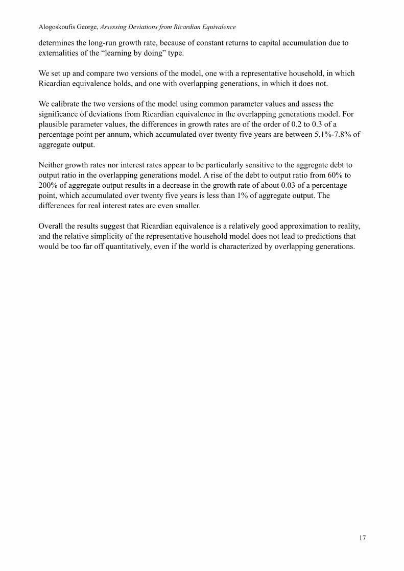
We calibrate the two versions of the model using common parameter values and assess the significance of deviations from Ricardian equivalence in the overlapping generations model. For plausible parameter values, the differences in growth rates are of the order of 0.2 to 0.3 of a percentage point per annum, which accumulated over twenty five years are between 5.1%-7.8% of aggregate output. Neither growth rates nor interest rates appear to be particularly sensitive to the aggregate debt to output ratio. A rise of the debt to output ratio from 60% to 200% of aggregate output results in a decrease in the growth rate of about 0.03 of a percentage point, which accumulated over twenty five years is less than 1% of aggregate output. The differences for real interest rates are even smaller. Overall the results suggest that Ricardian equivalence is a relatively good approximation to reality, and the relative simplicity of the representative household model does not lead to predictions that would be too far off quantitatively, even if the world is characterized by overlapping generations.

The rest of the paper is as follows: Section 1 uses a q model of investment, with convex adjustment costs, to characterize the investment decisions of firms. We assume learning by doing and constant returns to the accumulation of physical capital. In section 2 we model the relationship between the endogenous growth rate and the real interest rate, that is required for equilibrium investment. We show that the endogenous growth rate depends negatively on the real interest rate, and positively on the productivity of capital. In section 3 we introduce the government budget constraint and discuss alternative modes of financing government expenditure. In sections 4 and 5 we model private consumption behavior, using a representative household and an overlapping generations model respectively. In both the representative household model and the overlapping generations model, the endogenous growth rate and the real interest rate are co-determined through the interaction of equilibrium investment by firms and equilibrium savings by households. The assumption of adjustment costs for investment is crucial in this respect. Without investment adjustment costs, i.e with 𝜙=0, this co-determination does not apply in the endogenous growth model. The production side determines the real interest rate, as the net marginal product of capital, and, given the real interest rate, the consumption side determines the growth rate of consumption, capital and output. In section 6 we present the calibration results and section 7 sums up the conclusions.

1. The Investment Decisions of Firms

We assume an economy, consisting of a large number of competitive firms that produce a single homogeneous good.

2.1 Production

The production function of firm i at time t is given by,

Yit = AKitα (htLit )

1−α , 0<α<1 (1)

where Y is output, K physical capital, L the number of employees and h the efficiency of labour. The efficiency of labour is the same for all firms.


3

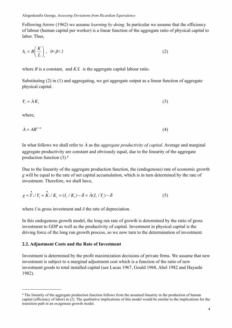
Following Arrow (1962) we assume learning by doing. In particular we assume that the efficiency of labour (human capital per worker) is a linear function of the aggregate ratio of physical capital to labor. Thus,

ht = BKL

⎛⎝⎜

⎞⎠⎟ t

, 0<β<1 (2)

where B is a constant, and K/L is the aggregate capital labour ratio.

Substituting (2) in (1) and aggregating, we get aggregate output as a linear function of aggregate physical capital.

Yt = A_Kt (3)

where,

A_= AB1−α (4)

In what follows we shall refer to A_

as the aggregate productivity of capital. Average and marginal aggregate productivity are constant and obviously equal, due to the linearity of the aggregate production function (3).4

Due to the linearity of the aggregate production function, the (endogenous) rate of economic growth g will be equal to the rate of net capital accumulation, which is in turn determined by the rate of investment. Therefore, we shall have,

g = Y•

t /Yt = K•

t / Kt = (It / Kt ) − δ = A_(It /Yt ) − δ (5)

where I is gross investment and δ the rate of depreciation.

In this endogenous growth model, the long run rate of growth is determined by the ratio of gross investment to GDP as well as the productivity of capital. Investment in physical capital is the driving force of the long run growth process, so we now turn to the determination of investment.

2.2. Adjustment Costs and the Rate of Investment

Investment is determined by the profit maximization decisions of private firms. We assume that new investment is subject to a marginal adjustment cost which is a function of the ratio of new investment goods to total installed capital (see Lucas 1967, Gould 1968, Abel 1982 and Hayashi 1982).


4

4 The linearity of the aggregate production function follows from the assumed linearity in the production of human capital (efficiency of labor) in (2). The qualitative implications of this model would be similar to the implications for the transition path in an exogenous growth model.

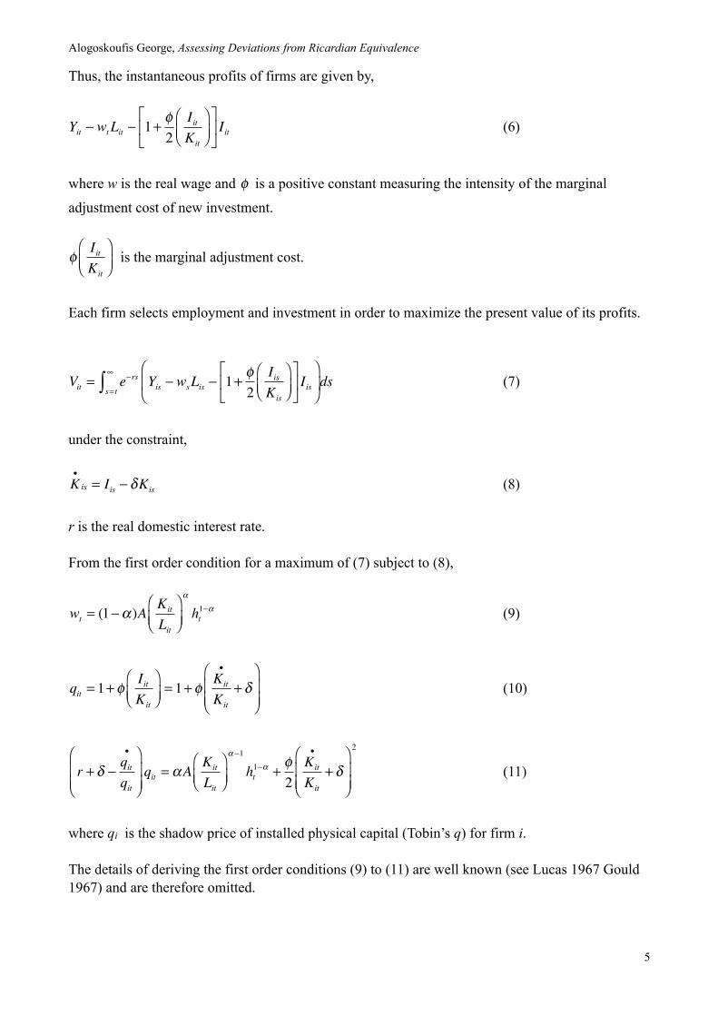
Thus, the instantaneous profits of firms are given by,

Yit − wtLit − 1+ φ2

IitKit

⎛⎝⎜

⎞⎠⎟

⎡

⎣⎢

⎤

⎦⎥ Iit (6)

where w is the real wage and φ is a positive constant measuring the intensity of the marginal

adjustment cost of new investment.

φ IitKit

⎛⎝⎜

⎞⎠⎟

is the marginal adjustment cost.

Each firm selects employment and investment in order to maximize the present value of its profits.

Vit = e−rs Yis − wsLis − 1+ φ2

IisKis

⎛⎝⎜

⎞⎠⎟

⎡

⎣⎢

⎤

⎦⎥ Iis

⎛

⎝⎜

⎞

⎠⎟s= t

∞

∫ ds (7)

under the constraint,

K•

is = Iis − δKis (8)

r is the real domestic interest rate.

From the first order condition for a maximum of (7) subject to (8),

wt = (1−α )AKit

Lit

⎛⎝⎜

⎞⎠⎟

α

ht1−α (9)

qit = 1+ φIitKit

⎛⎝⎜

⎞⎠⎟= 1+ φ Kit

•

Kit

+ δ⎛

⎝⎜⎜

⎞

⎠⎟⎟

(10)

r + δ −qit•

qit

⎛

⎝⎜⎜

⎞

⎠⎟⎟qit = αA

Kit

Lit

⎛⎝⎜

⎞⎠⎟

α −1

ht1−α +

φ2

Kit

•

Kit

+ δ⎛

⎝⎜⎜

⎞

⎠⎟⎟

2

(11)

where qi is the shadow price of installed physical capital (Tobin’s q) for firm i.

The details of deriving the first order conditions (9) to (11) are well known (see Lucas 1967 Gould 1967) and are therefore omitted.


5

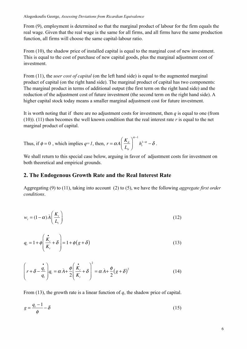
From (9), employment is determined so that the marginal product of labour for the firm equals the real wage. Given that the real wage is the same for all firms, and all firms have the same production function, all firms will choose the same capital-labour ratio.

From (10), the shadow price of installed capital is equal to the marginal cost of new investment. This is equal to the cost of purchase of new capital goods, plus the marginal adjustment cost of investment.

From (11), the user cost of capital (on the left hand side) is equal to the augmented marginal product of capital (on the right hand side). The marginal product of capital has two components: The marginal product in terms of additional output (the first term on the right hand side) and the reduction of the adjustment cost of future investment (the second term on the right hand side). A higher capital stock today means a smaller marginal adjustment cost for future investment.

It is worth noting that if there are no adjustment costs for investment, then q is equal to one (from (10)). (11) then becomes the well known condition that the real interest rate r is equal to the net marginal product of capital.

Thus, if φ = 0 , which implies q=1, then, r = αAKit

Lit

⎛⎝⎜

⎞⎠⎟

α −1

ht1−α − δ .

We shall return to this special case below, arguing in favor of adjustment costs for investment on both theoretical and empirical grounds.

2. The Endogenous Growth Rate and the Real Interest Rate

Aggregating (9) to (11), taking into account (2) to (5), we have the following aggregate first order conditions.

wt = (1−α )A_ Kt

Lt

⎛⎝⎜

⎞⎠⎟

(12)

qt = 1+ φKt

•

Kt

+ δ⎛

⎝⎜⎜

⎞

⎠⎟⎟= 1+ φ g + δ( ) (13)

r + δ −qt•

qt

⎛

⎝⎜⎜

⎞

⎠⎟⎟qt = α A

_+φ2

Kt

•

Kt

+ δ⎛

⎝⎜⎜

⎞

⎠⎟⎟

2

= α A_+φ2g + δ( )2 (14)

From (13), the growth rate is a linear function of q, the shadow price of capital.

g = qt −1φ

− δ (15)


6

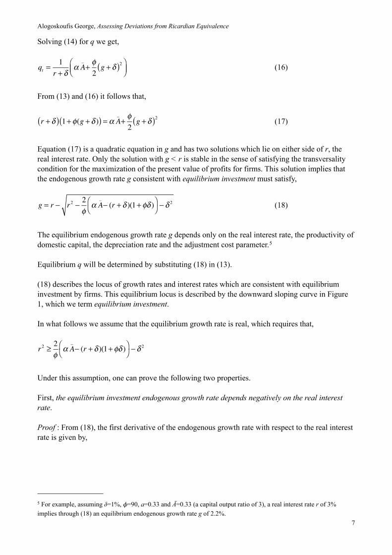
Solving (14) for q we get,

qt =1

r + δα A

_+φ2g + δ( )2⎛

⎝⎜⎞⎠⎟ (16)

From (13) and (16) it follows that,

r + δ( ) 1+ φ(g + δ )( ) = α A_+φ2g + δ( )2 (17)

Equation (17) is a quadratic equation in g and has two solutions which lie on either side of r, the real interest rate. Only the solution with g < r is stable in the sense of satisfying the transversality condition for the maximization of the present value of profits for firms. This solution implies that the endogenous growth rate g consistent with equilibrium investment must satisfy,

g = r − r2 − 2φ

α A_− (r + δ )(1+ φδ )⎛

⎝⎞⎠ − δ

2 (18)

The equilibrium endogenous growth rate g depends only on the real interest rate, the productivity of domestic capital, the depreciation rate and the adjustment cost parameter.5

Equilibrium q will be determined by substituting (18) in (13).

(18) describes the locus of growth rates and interest rates which are consistent with equilibrium investment by firms. This equilibrium locus is described by the downward sloping curve in Figure 1, which we term equilibrium investment.

In what follows we assume that the equilibrium growth rate is real, which requires that,

r2 ≥ 2φ

α A_− (r + δ )(1+ φδ )⎛

⎝⎞⎠ − δ

2

Under this assumption, one can prove the following two properties.

First, the equilibrium investment endogenous growth rate depends negatively on the real interest rate.

Proof : From (18), the first derivative of the endogenous growth rate with respect to the real interest rate is given by,


7

5 For example, assuming δ=1%, 𝜙=90, a=0.33 and Ā=0.33 (a capital output ratio of 3), a real interest rate r of 3% implies through (18) an equilibrium endogenous growth rate g of 2.2%.

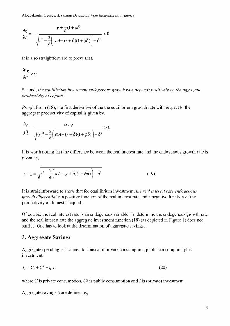
∂g∂r

= −g + 1

φ(1+ φδ )

r2 − 2φ

α A_− (r + δ )(1+ φδ )⎛

⎝⎞⎠ − δ

2

< 0

It is also straightforward to prove that,

∂2g∂r2

> 0

Second, the equilibrium investment endogenous growth rate depends positively on the aggregate productivity of capital.

Proof : From (18), the first derivative of the the equilibrium growth rate with respect to the aggregate productivity of capital is given by,

∂g

∂A_ =

α /φ

(r)2 − 2φ

α A_− (r + δ )(1+ φδ )⎛

⎝⎞⎠ − δ

2

> 0

It is worth noting that the difference between the real interest rate and the endogenous growth rate is given by,

r − g = r2 − 2φ

a A_− (r + δ )(1+ φδ )⎛

⎝⎞⎠ − δ

2 (19)

It is straightforward to show that for equilibrium investment, the real interest rate endogenous growth differential is a positive function of the real interest rate and a negative function of the productivity of domestic capital.

Of course, the real interest rate is an endogenous variable. To determine the endogenous growth rate and the real interest rate the aggregate investment function (18) (as depicted in Figure 1) does not suffice. One has to look at the determination of aggregate savings.

3. Aggregate Savings

Aggregate spending is assumed to consist of private consumption, public consumption plus investment.

Yt = Ct + Ctg + qt It (20)

where C is private consumption, Cg is public consumption and I is (private) investment.

Aggregate savings S are defined as,


8

St = Yt − Ct − Ctg (21)

Equilibrium requires that aggregate savings should be equal to investment. Thus,

St = Yt − Ct − Ctg = qt It (22)

Dividing (22) through by total output, we get,

st =StYt

= 1− ct − ctg = qt

ItYt

⎛⎝⎜

⎞⎠⎟=1

A_ 1+ φ(gt + δ )( )(gt + δ ) (23)

where c=C/Y is the share of private consumption in total output and cg=Cg/Y is the share of public consumption in total output.

To determine the aggregate savings rate, we have to look at the consumption decisions of households and the government.

4. Government Debt and the Government Budget Constraint

We start with the government. We shall assume that government consumption can be financed either through lump-sum taxes, or through government debt.

The evolution of the public debt to output ratio is determined by,

b•

t = rt − gt( )bt + ctg − τ t (24)

where b is the debt to output ratio and τ is the ratio of total current (lump sum tax) revenue to output.

Since the real interest rate exceeds the output growth rate, the debt to output ratio increases without limit, unless there is a primary suplus that exactly offsets interest payments on the existing debt.

In what follows we shall assume that the government consumption to output ratio is constant and that the government adjusts total current revenue to achieve a primary surplus that stabilizes the public debt to output ratio.

From (24), this means that,

b_=τ t − c

g_

rt − gt (25)

The bar over b and cg denotes the government targets for public debt and public consumption respectively.


9

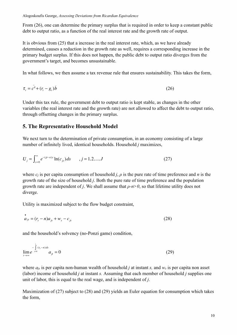
From (26), one can determine the primary surplus that is required in order to keep a constant public debt to output ratio, as a function of the real interest rate and the growth rate of output.

It is obvious from (25) that a increase in the real interest rate, which, as we have already determined, causes a reduction in the growth rate as well, requires a corresponding increase in the primary budget surplus. If this does not happen, the public debt to output ratio diverges from the government’s target, and becomes unsustainable.

In what follows, we then assume a tax revenue rule that ensures sustainability. This takes the form,

τ t = cg_

+ (rt − gt )b_

(26)

Under this tax rule, the government debt to output ratio is kept stable, as changes in the other variables (the real interest rate and the growth rate) are not allowed to affect the debt to output ratio, through offsetting changes in the primary surplus.

5. The Representative Household Model

We next turn to the determination of private consumption, in an economy consisting of a large number of infinitely lived, identical households. Household j maximizes,

Uj = e−(ρ−n)s ln(cjs )dss=0

∞

∫ , j = 1,2,..., J (27)

where cj is per capita consumption of household j, ρ is the pure rate of time preference and n is the growth rate of the size of household j. Both the pure rate of time preference and the population growth rate are independent of j. We shall assume that ρ-n>0, so that lifetime utility does not diverge.

Utility is maximized subject to the flow budget constraint,

a•

js = (rs − n)ajs + ws − cjs (28)

and the household’s solvency (no-Ponzi game) condition,

limt→∞

e− (rs −n)dss=0

t

∫ajt = 0 (29)

where ajs is per capita non-human wealth of household j at instant s, and ws is per capita non asset (labor) income of household j at instant s. Assuming that each member of household j supplies one unit of labor, this is equal to the real wage, and is independent of j.

Maximization of (27) subject to (28) and (29) yields an Euler equation for consumption which takes the form,


10

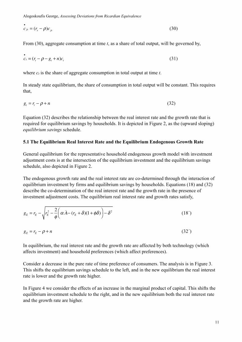
c•

js = (rs − ρ)cjs (30)

From (30), aggregate consumption at time t, as a share of total output, will be governed by,

c•

t = (rt − ρ − gt + n)ct (31)

where ct is the share of aggregate consumption in total output at time t.

In steady state equilibrium, the share of consumption in total output will be constant. This requires that,

gt = rt − ρ + n (32)

Equation (32) describes the relationship between the real interest rate and the growth rate that is required for equilibrium savings by households. It is depicted in Figure 2, as the (upward sloping) equilibrium savings schedule.

5.1 The Equilibrium Real Interest Rate and the Equilibrium Endogenous Growth Rate

General equilibrium for the representative household endogenous growth model with investment adjustment costs is at the intersection of the equilibrium investment and the equilibrium savings schedule, also depicted in Figure 2.

The endogenous growth rate and the real interest rate are co-determined through the interaction of equilibrium investment by firms and equilibrium savings by households. Equations (18) and (32) describe the co-determination of the real interest rate and the growth rate in the presence of investment adjustment costs. The equilibrium real interest rate and growth rates satisfy,

gE = rE − rE2 −2φ

α A_− (rE + δ )(1+ φδ )

⎛⎝

⎞⎠ − δ

2 (18΄)

gE = rE − ρ + n (32΄)

In equilibrium, the real interest rate and the growth rate are affected by both technology (which affects investment) and household preferences (which affect preferences).

Consider a decrease in the pure rate of time preference of consumers. The analysis is in Figure 3. This shifts the equilibrium savings schedule to the left, and in the new equilibrium the real interest rate is lower and the growth rate higher.

In Figure 4 we consider the effects of an increase in the marginal product of capital. This shifts the equilibrium investment schedule to the right, and in the new equilibrium both the real interest rate and the growth rate are higher.


11

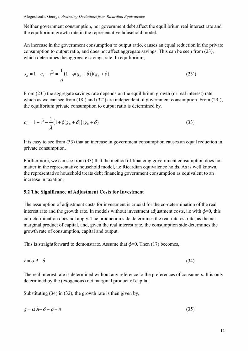
Neither government consumption, nor government debt affect the equilibrium real interest rate and the equilibrium growth rate in the representative household model.

An increase in the government consumption to output ratio, causes an equal reduction in the private consumption to output ratio, and does not affect aggregate savings. This can be seen from (23), which determines the aggregate savings rate. In equilibrium,

sE = 1− cE − cg_

=1

A_ 1+ φ(gE + δ )( )(gE + δ ) (23΄)

From (23΄) the aggregate savings rate depends on the equilibrium growth (or real interest) rate, which as we can see from (18΄) and (32΄) are independent of government consumption. From (23΄), the equilibrium private consumption to output ratio is determined by,

cE = 1− cg_

−1

A_ 1+ φ(gE + δ )( )(gE + δ ) (33)

It is easy to see from (33) that an increase in government consumption causes an equal reduction in private consumption.

Furthermore, we can see from (33) that the method of financing government consumption does not matter in the representative household model, i.e Ricardian equivalence holds. As is well known, the representative household treats debt financing government consumption as equivalent to an increase in taxation.

5.2 The Significance of Adjustment Costs for Investment

The assumption of adjustment costs for investment is crucial for the co-determination of the real interest rate and the growth rate. In models without investment adjustment costs, i.e with 𝜙=0, this co-determination does not apply. The production side determines the real interest rate, as the net marginal product of capital, and, given the real interest rate, the consumption side determines the growth rate of consumption, capital and output.

This is straightforward to demonstrate. Assume that 𝜙=0. Then (17) becomes,

r = α A_− δ (34)

The real interest rate is determined without any reference to the preferences of consumers. It is only determined by the (exogenous) net marginal product of capital.

Substituting (34) in (32), the growth rate is then given by,

g = α A_− δ − ρ + n (35)


12

Equations (34) and (35) describe the determination of the real interest rate and the growth rate in the absence of adjustment costs for investment. Unlike our more general model, without adjustment costs, the real interest rate does not depend on household preferences, but only on the exogenous net marginal product of capital.

6. The Overlapping Generations Model

We next turn to an alternative overlapping generations model for the determination of private consumption. We shall assume a model in which population growth comes in the form of entry of new households into the economy. Thus households differ by their date of birth. All households are infinitely lived, but each generation is only concerned about its own welfare and not the welfare of forthcoming generations.

nLt households are born at each instant, where Lt is total population at instant t, and n is the rate of growth of the number of households (and population). We shall further assume that each household supplies one unit of labor. Therefore n is also the rate of growth of the labor force.

The household born at instant j chooses chooses consumption to maximize,

Uj = e−ρs ln(cjs )dss= j

∞

∫ (36)

subject to the instantaneous budget constraint,

a•

js = rsajs + wjs − cjs (37)

and the household’s solvency (no-Ponzi game) condition,

limt→∞

e− rs dss= j

t

∫ajt = 0 (38)

Maximization of (36) subject to (37) and (38) yields an Euler equation for consumption which takes the form,

c•

js = (rs − ρ)cjs (39)

We can use the first order condition (36) to derive aggregate consumption. From (39) and the household’s present value budget constraint it follows that,

cjs = ρ ajs + wjve− rψ dψ

ψ =s

ν

∫ dνν= s

∞

∫⎛

⎝⎜⎞

⎠⎟ (40)

Consumption is linear in total wealth because of the assumption of the constant elasticity of inter-temporal substitution. Furthermore, as we have assumed that the elasticity of inter-temporal


13

substitution is equal to 1, the propensity to consume out of wealth is independent of the real interest rate and only depends on the pure rate of time preference.

The size of the cohort born at time j equals nLj, where Lj=exp(nj) is the population size at time j. Population aggregates are defined as,

Ct = n cjtenj dj

j=−∞

t

∫ (41)

Aggregating over cohorts, assuming that newly born households do not inherit any wealth, yields,

C•

t = (rt − ρ + n)Ct − nρAt (42)

where C is aggregate consumption and A is aggregate household non-human wealth.

Equation (42) determines the evolution of aggregate consumption. Dividing (39) by total output Y, yields,

c•

t = (rt − gt − ρ + n)ct − nρ (qt / A_)+ b

_⎛⎝

⎞⎠ (43)

In (43) we have assumed that all household non-human wealth is held in the form of government bonds and shares in domestic firms. The value of shares is equal to qK. It then follows from the aggregate production function (3), that,

qtKt

Yt= qt / A

_ (44)

From (43), in steady state equilibrium,

cE =nρ

(rE − gE − ρ + n)(qE A

_)+ b

_⎛⎝

⎞⎠ (45)

From (23), aggregate savings as a share of output is given by,

sE = 1− cE − cg_

= 1− nρ(rE − gE − ρ + n)

(qE / A_)+ b

_⎛⎝

⎞⎠ − c

g_

(23΄΄)

Using (13) to substitute for qE in (23΄΄), we get,

sE = 1− cE − cg_

= 1− nρ(rE − gE − ρ + n)

1+φ(gE +δ )

A_ + b

_⎛

⎝⎜

⎞

⎠⎟ − c

g_

(46)


14

Equation (46) describes the relationship between the real interest rate and the growth rate that is required for equilibrium savings by households. It is the equivalent of (32΄) for the representative household model.

The slope of the equilibrium savings locus is given by,

0 < dgdr

=nρ 1+ φ(g + δ )( )

nρ 1+ φ(g + δ )( ) + nρφ(r − g − ρ + n)< 1 (47)

The equilibrium savings locus has a positive slope. However, the slope is lower than one, which is the slope of the comparable representative household model. In addition it is straightforward to show that the slope is declining in the real interest rate. The equilibrium savings locus lies to the right of the equilibrium savings locus of the comparable representative household model, as for any growth rate, the real interest rate is higher.

In addition, the equilibrium savings locus depends negatively on both government consumption and government debt relative to output. Both government expenditure and its mode of finance matter for aggregate savings. Higher government expenditure requires higher current and future taxation as a share of output. However, because part of the future taxation will be shouldered by as yet unborn generations, a rise in government expenditure reduces aggregate savings. The reduction in private consumption is smaller than the rise in government consumption. For the same reason, Ricardian equivalence does not hold. Government debt is considered as wealth by current generations, as the rise in lump sum taxes to finance the servicing of the debt will be partly shouldered by future generations.

The equilibrium savings locus (46) is depicted in Figure 5, along with the equilibrium savings schedule of the comparable representative household model. It is easy to see that the real interest rate is higher and the growth rate is lower in the overlapping generations (OLG) case than in the comparable representative household (RH) model.

As in the representative household model, in the overlapping generations model, the endogenous growth rate and the real interest rate are co-determined through the interaction of equilibrium investment by firms and equilibrium savings by households. However, unlike the case of the representative household model, government expenditure and the way it is financed matters in this case. An increase in either government expenditure relative to output, or government debt, will shift the equilibrium savings locus to the right. This will result in a rise in the real interest rate and a reduction in the growth rate.

The analysis is in Figure 6. A rise in the government debt to output ratio reduces private and aggregate savings, and shifts the equilibrium savings locus to the right. In the new equilibrium, the real interest rate is higher and the growth rate is lower, as the fall in savings causes a fall in investment. Similar effects would arise following a rise in the government consumption to output ratio, as the fall in private consumption would be smaller than the rise in government consumption. Such effects would not arise in the corresponding representative household model (RH) in which Ricardian equivalence holds.


15

The assumption of adjustment costs for investment is again crucial. Without investment adjustment costs, i.e with 𝜙=0, the co-determination of the growth rate and the real interest rate does not apply in the endogenous growth model. The production side determines the real interest rate, as the net marginal product of capital, and, given the real interest rate, the consumption side determines the growth rate of consumption, capital and output.

6.Assessing Deviations from Ricardian Equivalence

We have seen that the overlapping generations model implies a distortion that results in higher real interest rates and lower endogenous growth rates. This distortion arises from the fact that current households do not provide for the welfare of future generations. How important is this distortion; This is the question to which we now turn.

In order to assess the magnitude of this distortion, we calibrate the two alternative models, using a common set of parameter values. We assume that the share of labor in the production function is equal to one third (α=0.33), that the capital output ratio is equal to 3 (aggregate productivity of capital equal to 0.33), that the depreciation rate is equal to 1%, the population growth rate is equal to 1%, that the share of government consumption to output is 20% and that the adjustment cost parameter is equal to 50. The results for the representative household model, with the pure rate of time preference ranging from 2% to 4% are presented in Table 1.

In Table 2 we present results for the overlapping generations model, assuming the same values for all parameters, a pure rate of time preference of 3%, and a government debt to output ratio ranging from 0 to 500% of output.

As can be seen by comparing the two tables, the differences between the representative household model and the overlapping generations model are quantitatively relatively small. As predicted by the theory, the overlapping generations model results in higher consumption, higher interest rates and lower growth rates. However, the differences are of the order of 0.2-0.3 of a percentage point for the aggregate growth rate, 0.3-0.4% for the aggregate savings rate, and even smaller for the real interest rate. A difference of 0.2 of a percentage point in the growth rate, accumulated over 25 years, would result in a output which is higher by 5.1%. This is not insignificant, but economies often experience larger output losses during recessions.

Neither growth rates nor interest rates appear to be particularly sensitive to the aggregate debt to output ratio. A rise of the debt to output ratio from 60% to 200% of aggregate output results in a decrease in the growth rate of about 0.03 of a percentage point, which accumulated over twenty five years is less than 1% of aggregate output. The differences for real interest rates are even smaller. Overall the results suggest that Ricardian equivalence is a relatively good approximation to reality, and the relative simplicity of the representative household model does not lead to predictions that would be too far off quantitatively, even if the world is characterized by overlapping generations.

7.Conclusions

This paper proposes a method for assessing the quantitative significance of deviations from the Ricardian equivalence hypothesis. The model proposed for this purpose belongs to a class of endogenous growth theories with investment adjustment costs, in which savings and investment are co-determined through adjustments in the real interest rate. The equilibrium investment rate


16

determines the long-run growth rate, because of constant returns to capital accumulation due to externalities of the “learning by doing” type.

We set up and compare two versions of the model, one with a representative household, in which Ricardian equivalence holds, and one with overlapping generations, in which it does not.

We calibrate the two versions of the model using common parameter values and assess the significance of deviations from Ricardian equivalence in the overlapping generations model. For plausible parameter values, the differences in growth rates are of the order of 0.2 to 0.3 of a percentage point per annum, which accumulated over twenty five years are between 5.1%-7.8% of aggregate output.

Neither growth rates nor interest rates appear to be particularly sensitive to the aggregate debt to output ratio in the overlapping generations model. A rise of the debt to output ratio from 60% to 200% of aggregate output results in a decrease in the growth rate of about 0.03 of a percentage point, which accumulated over twenty five years is less than 1% of aggregate output. The differences for real interest rates are even smaller.

Overall the results suggest that Ricardian equivalence is a relatively good approximation to reality, and the relative simplicity of the representative household model does not lead to predictions that would be too far off quantitatively, even if the world is characterized by overlapping generations.


17

Table 1Calibration of the Representative Household Model

ρ c r g

2,0% 76,09% 3,97% 2,97%

2,5% 76,73% 4,06% 2,56%

3,0% 77,28% 4,18% 2,18%

3,5% 77,73% 4,34% 1,84%

4,0% 78,12% 4,52% 1,52%

Note: We assume that α=0.33, Ᾱ=0.33, 𝜙=50, δ=1%, n=1% and cg=20%. The calculations have been performed using the Wolfram Alpha computational knowledge engine.See http://www.wolframalpha.com .


18

http://www.wolframalpha.com


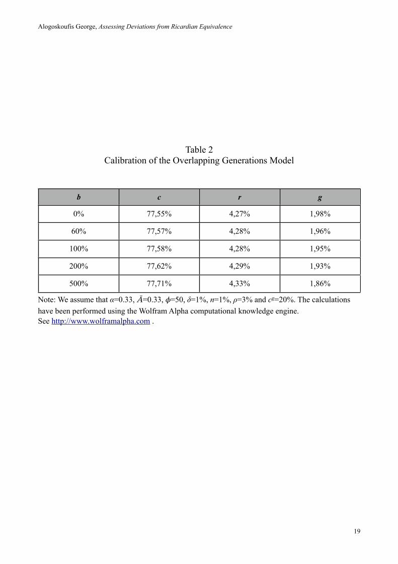
Table 2Calibration of the Overlapping Generations Model

b c r g

0% 77,55% 4,27% 1,98%

60% 77,57% 4,28% 1,96%

100% 77,58% 4,28% 1,95%

200% 77,62% 4,29% 1,93%

500% 77,71% 4,33% 1,86%

Note: We assume that α=0.33, Ᾱ=0.33, 𝜙=50, δ=1%, n=1%, ρ=3% and cg=20%. The calculations have been performed using the Wolfram Alpha computational knowledge engine.See http://www.wolframalpha.com .


19



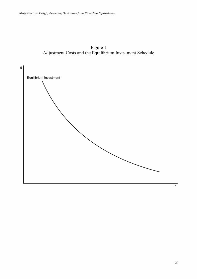
Figure 1Adjustment Costs and the Equilibrium Investment Schedule

g

r

Equilibrium Investment


20

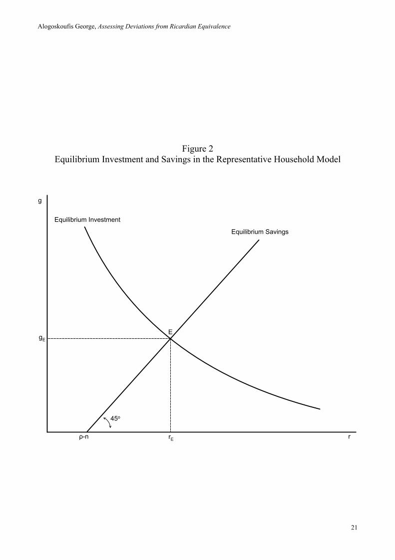
Figure 2Equilibrium Investment and Savings in the Representative Household Model

g

r


Equilibrium Savings

ρ-n

45o

gE

rE

E


21

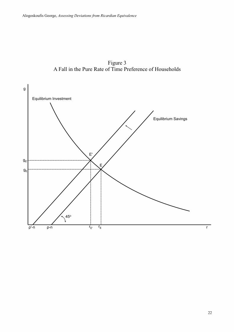
Figure 3A Fall in the Pure Rate of Time Preference of Households

g

r


Equilibrium Savings

ρ-n

45o

gE

rE

E

ρ'-n

E'gE'

rE'


22

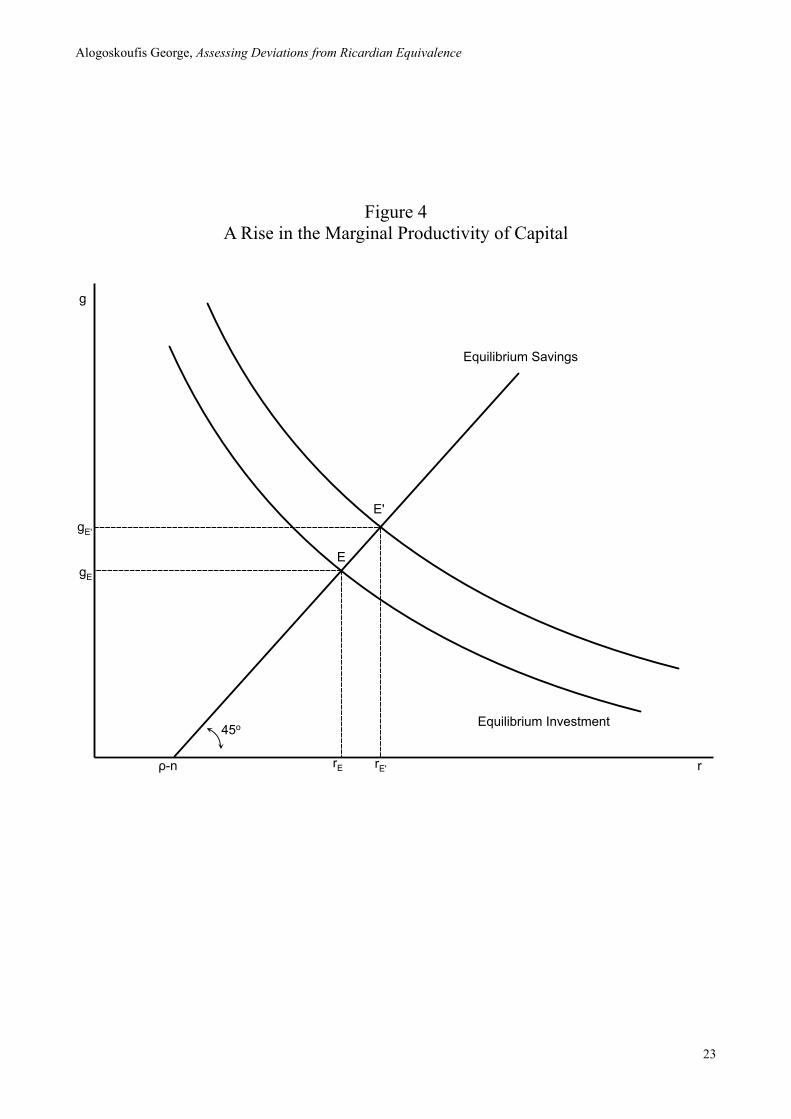
Figure 4A Rise in the Marginal Productivity of Capital

g

r


Equilibrium Savings

ρ-n

45o

gE

rE

E

E'

rE'

gE'


23

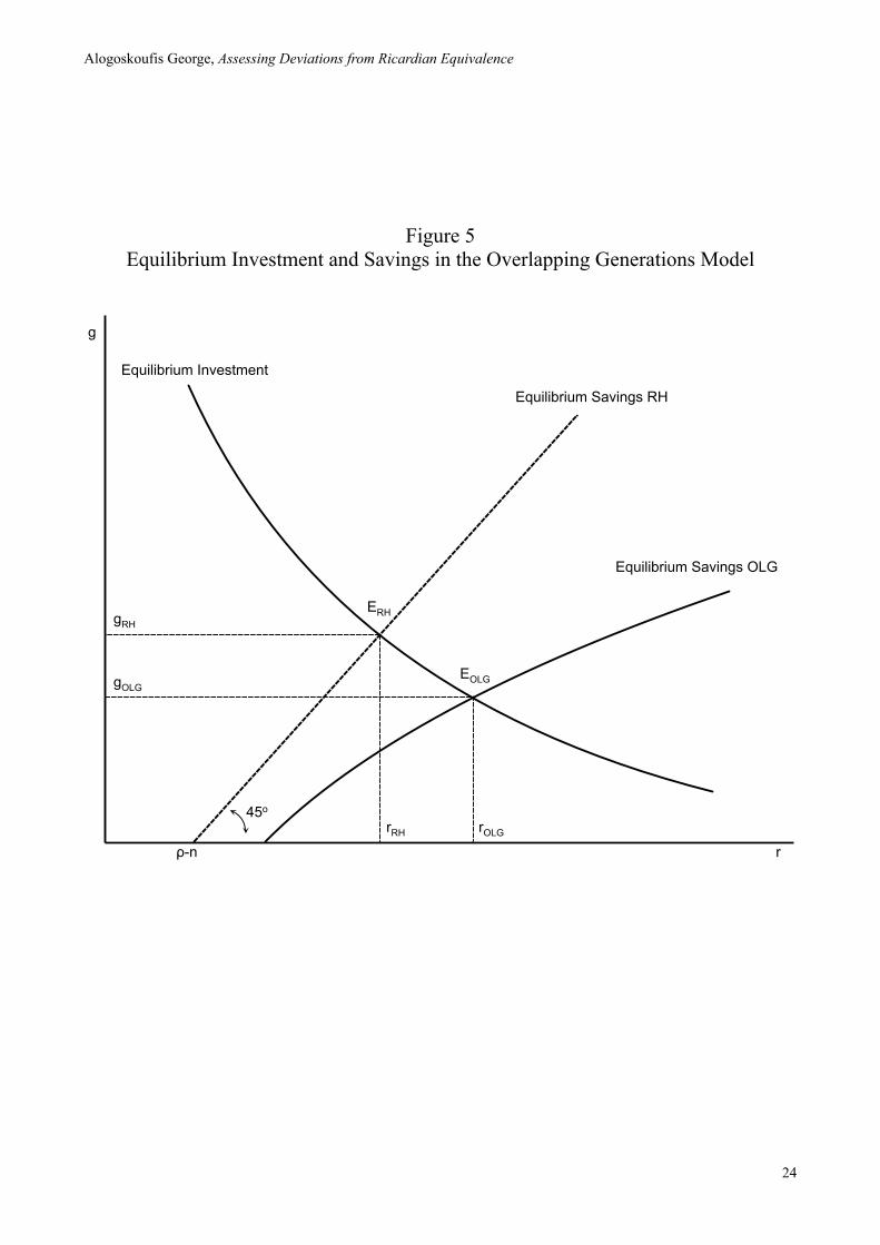
Figure 5Equilibrium Investment and Savings in the Overlapping Generations Model

g

r


Equilibrium Savings RH

ρ-n

45o

gRH

rRH

ERH

Equilibrium Savings OLG

EOLGgOLG

rOLG


24

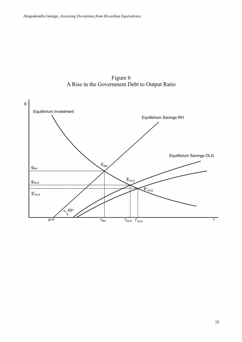
Figure 6A Rise in the Government Debt to Output Ratio

g

r

Equilibrium InvestmentEquilibrium Savings RH

ρ-n

45o

gRH

rRH

ERH

Equilibrium Savings OLG

EOLGgOLG

rOLG

g'OLG

E'OLG

r'OLG


25

References

Abel A.B. (1982), “Dynamic Effects of Permanent and Temporary Tax Policies in a q model of Investment”, Journal of Monetary Economics, 9, pp. 353-373.

Acemoglou D. (2009), Modern Economic Growth, Princeton N.J., Princeton University Press.Aghion P. and Howitt P. (2009), The Economics of Growth, Cambridge Mass., MIT Press.Arrow K.J. (1962), “The Economic Implications of Learning by Doing”, Review of Economic

Studies, 29, pp. 155-173.Barro R.J. (1974), “Are Government Bonds Net Wealth?”, Journal of Political Economy, 82, pp.

1095-1117.Barro R.J. and Sala-i-Martin X. (2004), Economic Growth, (2nd Edition), Cambridge Mass., MIT

Press.Blanchard O.J. (1985), “Debts, Deficits and Finite Horizons”, Journal of Political Economy, 93, pp.

223-247.Cass D. (1965), “Optimum Growth in an Aggregative Model of Capital Accumulation”, Review of

Economic Studies, 32, pp. 233-240.Diamond P. (1965), “National Debt in a Neoclassical Growth Model”, American Economic Review,

55, pp. 1126-1150.Gould J.P. (1968), “Adjustment Costs in the Theory of Investment of the Firm”, Review of

Economic Studies, 35, pp. 47-55.Hayashi F. (1982), “Tobin’s Marginal q and Average q: A Neoclassical Interpretation”,

Econometrica, 50, pp. 213-224.Koopmans T.C. (1965), “On the Concept of Optimal Economic Growth”, in the Economic

Approach To Development Planning, Amsterdam, Elsevier.Lucas R.E. Jr (1967), “Adjustment Costs and the Theory of Supply”, Journal of Political Economy,

75, pp. 321-334. Lucas R.E. Jr (1988), “On the Mechanics of Economic Development”, Journal of Monetary

Economics, 22, pp. 3-42.Ramsey F. (1928), “A Mathematical Theory of Saving”, Economic Journal, 38, pp. 543-559.Romer P. (1986), “Increasing Returns and Long Run Growth”, Journal of Political Economy, 94,

pp. 1002-1037. Solow R.M. (1956), “A Contribution to the Theory of Economic Growth”, Quarterly Journal of

Economics, 70, pp. 65-94.Tobin J. (1969), “A General Equilibrium Approach to Monetary Theory”, Journal of Money, Credit

and Banking, 1, pp. 15-29.Weil P. (1989), “Overlapping Families of Infinitely Lived Households”, Journal of Public

Economics, 38, pp. 183-198.


26

Documents

Assessing Ricardian Equivalence in an Endogenous Growth … · Lucas 1967, Gould 1968, Tobin 1969, Abel 1982, Hayashi 1982). In this theory, it is assumed that firms face convex internal