Embed Size (px)
Citation preview
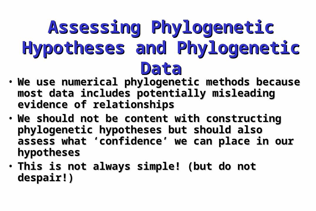
Assessing Phylogenetic Assessing Phylogenetic Hypotheses and Phylogenetic Hypotheses and Phylogenetic
DataData• We use numerical phylogenetic methods We use numerical phylogenetic methods
because most data includes potentially because most data includes potentially misleading evidence of relationshipsmisleading evidence of relationships
• We should not be content with constructing We should not be content with constructing phylogenetic hypotheses but should also phylogenetic hypotheses but should also assess what ‘confidence’ we can place in our assess what ‘confidence’ we can place in our hypotheseshypotheses
• This is not always simple! (but do not This is not always simple! (but do not despair!)despair!)
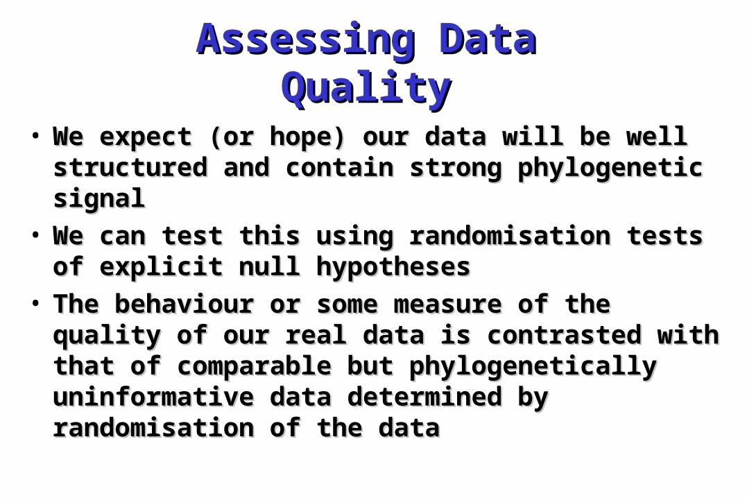
Assessing Data QualityAssessing Data Quality
• We expect (or hope) our data will be well We expect (or hope) our data will be well structured and contain strong phylogenetic structured and contain strong phylogenetic signalsignal
• We can test this using randomisation tests of We can test this using randomisation tests of explicit null hypothesesexplicit null hypotheses
• The behaviour or some measure of the quality The behaviour or some measure of the quality of our real data is contrasted with that of of our real data is contrasted with that of comparable but phylogenetically comparable but phylogenetically uninformative data determined by uninformative data determined by randomisation of the datarandomisation of the data
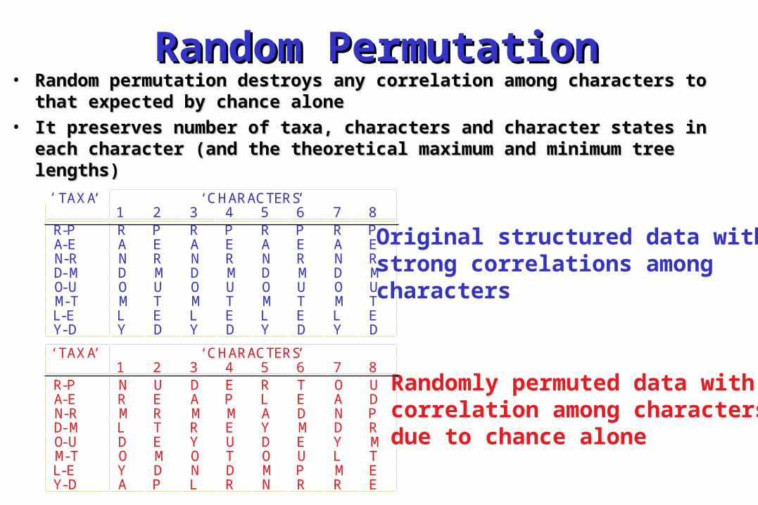
Random PermutationRandom Permutation• Random permutation destroys any correlation among characters to Random permutation destroys any correlation among characters to
that expected by chance alonethat expected by chance alone• It preserves number of taxa, characters and character states in It preserves number of taxa, characters and character states in
each character (and the theoretical maximum and minimum tree each character (and the theoretical maximum and minimum tree lengths)lengths)
Original structured data withstrong correlations amongcharacters
‘TAXA’ ‘CHARACTERS’1 2 3 4 5 6 7 8
R-P N U D E R T O UA-E R E A P L E A DN-R M R M M A D N PD-M L T R E Y M D RO-U D E Y U D E Y MM-T O M O T O U L TL-E Y D N D M P M EY-D A P L R N R R E
Randomly permuted data with correlation among charactersdue to chance alone
‘ TAXA’ ‘CHARACTERS’1 2 3 4 5 6 7 8
R-P R P R P R P R PA-E A E A E A E A EN-R N R N R N R N RD-M D M D M D M D MO-U O U O U O U O UM-T M T M T M T M TL-E L E L E L E L EY-D Y D Y D Y D Y D
Matrix Randomisation Matrix Randomisation TestsTests• Compare some measure of data quality Compare some measure of data quality
(hierarchical structure) for the real and (hierarchical structure) for the real and many randomly permuted data setsmany randomly permuted data sets
• This allows us to define a This allows us to define a test statistictest statistic for the null hypothesis that the real data for the null hypothesis that the real data are no better structured than randomly are no better structured than randomly permuted and phylogenetically permuted and phylogenetically uninformative datauninformative data
• A A permutation tail probabilitypermutation tail probability ((PTPPTP) is ) is the proportion of data sets with as good the proportion of data sets with as good or better measure of quality than the or better measure of quality than the real datareal data
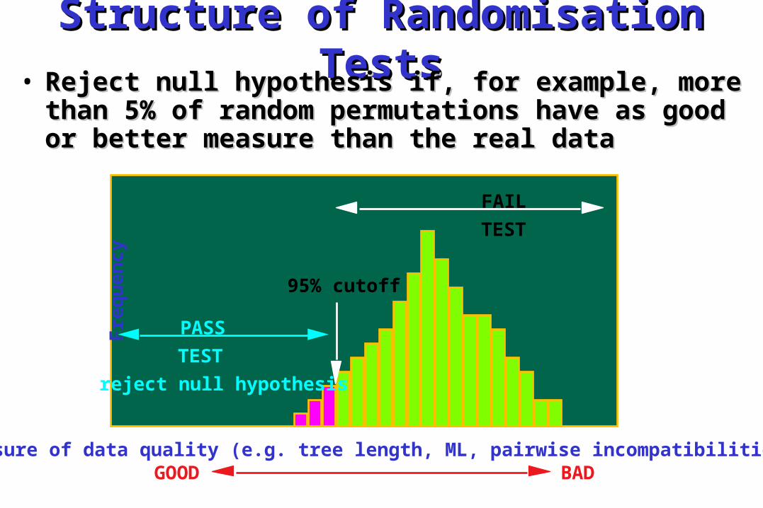
Structure of Randomisation Structure of Randomisation TestsTests• Reject null hypothesis if, for example, more Reject null hypothesis if, for example, more
than 5% of random permutations have as good than 5% of random permutations have as good or better measure than the real dataor better measure than the real data
Measure of data quality (e.g. tree length, ML, pairwise incompatibilities)
95% cutoff
GOOD BAD
F
req
ue
ncy
PASS
TEST
reject null hypothesis
FAIL
TEST
Matrix Randomisation Matrix Randomisation TestsTests
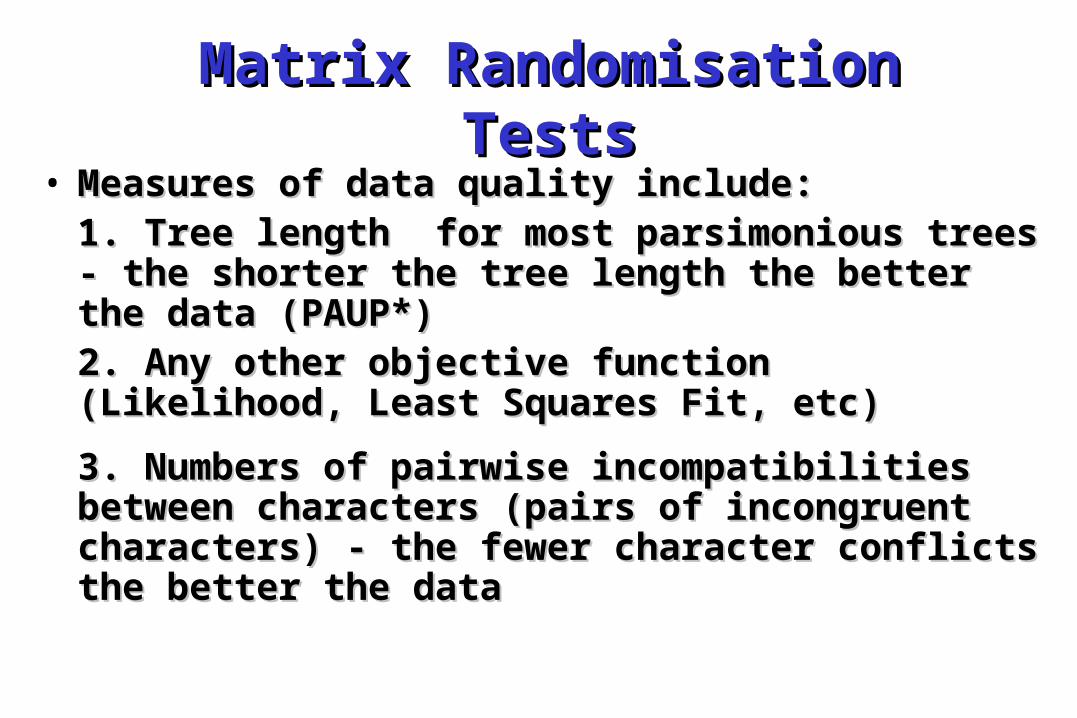
• Measures of data quality include:Measures of data quality include: 1. Tree length for most parsimonious trees - 1. Tree length for most parsimonious trees -
the shorter the tree length the better the the shorter the tree length the better the data (PAUP*)data (PAUP*)
2. Any other objective function (Likelihood, 2. Any other objective function (Likelihood, Least Squares Fit, etc)Least Squares Fit, etc)
3. Numbers of pairwise incompatibilities 3. Numbers of pairwise incompatibilities between characters (pairs of incongruent between characters (pairs of incongruent characters) - the fewer character conflicts characters) - the fewer character conflicts the better the datathe better the data
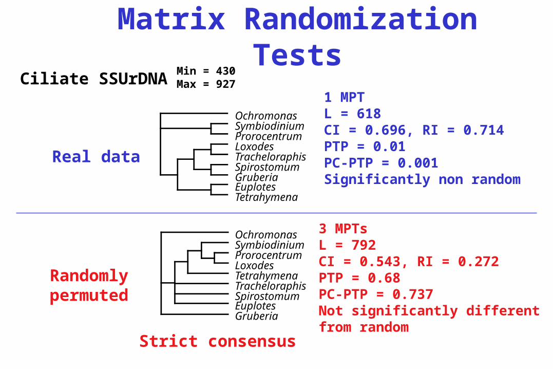
Matrix Randomization Tests
Real data
Randomly permuted
Ciliate SSUrDNA
Strict consensus
1 MPTL = 618CI = 0.696, RI = 0.714PTP = 0.01PC-PTP = 0.001Significantly non random
3 MPTsL = 792CI = 0.543, RI = 0.272PTP = 0.68PC-PTP = 0.737Not significantly differentfrom random
Min = 430Max = 927
OchromonasSymbiodiniumProrocentrumLoxodesTracheloraphisSpirostomumGruberiaEuplotesTetrahymena
OchromonasSymbiodiniumProrocentrumLoxodesTetrahymenaTracheloraphisSpirostomumEuplotesGruberia
Matrix Randomisation Tests - Matrix Randomisation Tests - use and limitationsuse and limitations
• Can detect very poor data - that Can detect very poor data - that provides no good basis for provides no good basis for phylogenetic inferences (throw it phylogenetic inferences (throw it away!)away!)
• However, only very little may be However, only very little may be needed to reject the null hypothesis needed to reject the null hypothesis (passing test (passing test great data) great data)
• Doesn’t indicate location of this Doesn’t indicate location of this structure (more discerning tests are structure (more discerning tests are possible)possible)
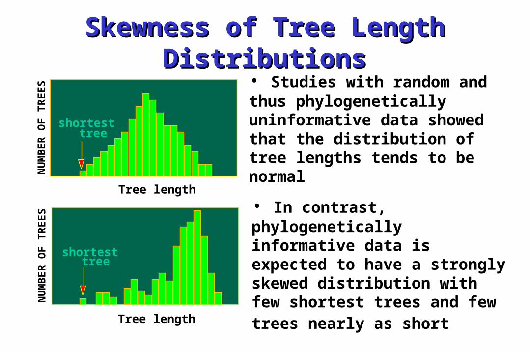
Skewness of Tree Length Skewness of Tree Length DistributionsDistributions
• Studies with random and thus phylogenetically uninformative data showed that the distribution of tree lengths tends to be normal
• In contrast, phylogenetically informative data is expected to have a strongly skewed distribution with few shortest trees and few trees nearly as short
NU
MB
ER
OF
TR
EE
S
shortest tree
NU
MB
ER
OF
TR
EE
S
shortest tree
Tree length
Tree length
Skewness of Tree Length Skewness of Tree Length DistributionsDistributions
• Measured with the GMeasured with the G11 statistic (PAUP*) statistic (PAUP*)
• Skewness of tree length distributions Skewness of tree length distributions could be used as a measure of data could be used as a measure of data quality in a randomisation testquality in a randomisation test
• Significance cut-offs for data sets of up Significance cut-offs for data sets of up to eight taxa have been published based to eight taxa have been published based on randomly generated data (rather on randomly generated data (rather than randomly permuted data)than randomly permuted data)
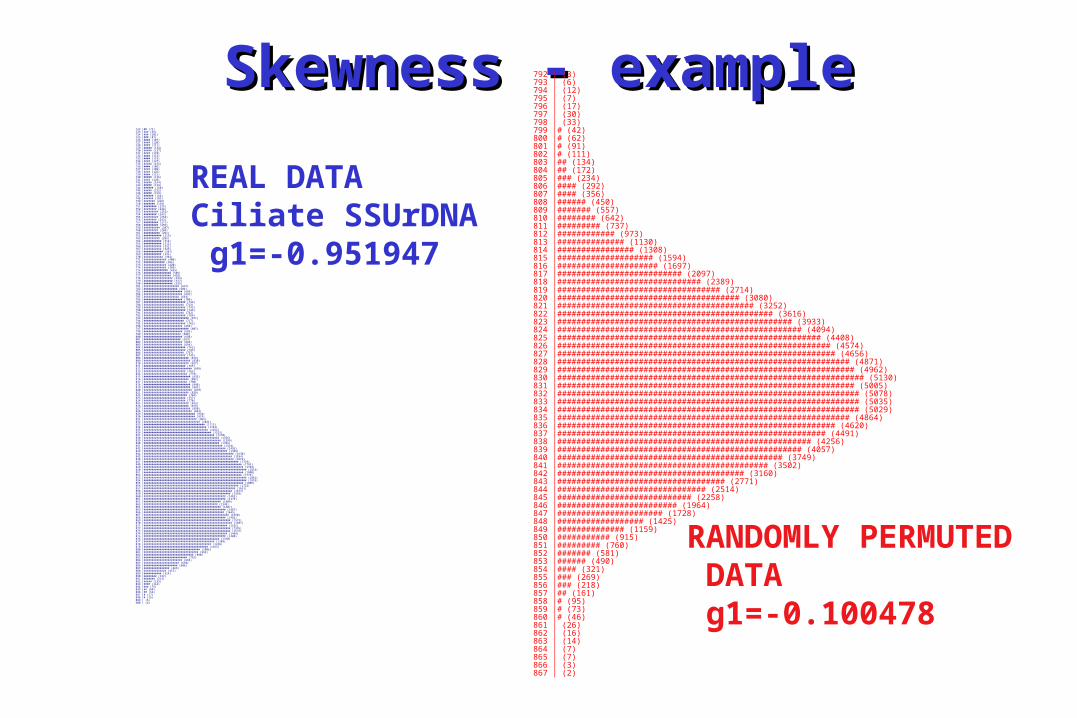
Skewness - exampleSkewness - example792 | (3)793 | (6)794 | (12)795 | (7)796 | (17)797 | (30)798 | (33)799 |# (42)800 |# (62)801 |# (91)802 |# (111)803 |## (134)804 |## (172)805 |### (234)806 |#### (292)807 |#### (356)808 |###### (450)809 |####### (557)810 |######## (642)811 |######### (737)812 |############ (973)813 |############## (1130)814 |################ (1308)815 |#################### (1594)816 |##################### (1697)817 |########################## (2097)818 |############################## (2389)819 |################################## (2714)820 |###################################### (3080)821 |######################################### (3252)822 |############################################# (3616)823 |################################################# (3933)824 |################################################### (4094)825 |####################################################### (4408)826 |######################################################### (4574)827 |########################################################## (4656)828 |############################################################# (4871)829 |############################################################## (4962)830 |################################################################ (5130)831 |############################################################## (5005)832 |############################################################### (5078)833 |############################################################### (5035)834 |############################################################### (5029)835 |############################################################# (4864)836 |########################################################## (4620)837 |######################################################## (4491)838 |##################################################### (4256)839 |################################################### (4057)840 |############################################### (3749)841 |############################################ (3502)842 |####################################### (3160)843 |################################### (2771)844 |############################### (2514)845 |############################ (2258)846 |######################### (1964)847 |###################### (1728)848 |################## (1425)849 |############## (1159)850 |########### (915)851 |######### (760)852 |####### (581)853 |###### (490)854 |#### (321)855 |### (269)856 |### (218)857 |## (161)858 |# (95)859 |# (73)860 |# (46)861 | (26)862 | (16)863 | (14)864 | (7)865 | (7)866 | (3)867 | (2)
RANDOMLY PERMUTED DATA g1=-0.100478
722 |## (72)723 |### (92)724 |### (101)725 |### (87)726 |#### (107)727 |#### (120)728 |#### (111)729 |##### (134)730 |##### (137)731 |#### (110)732 |#### (113)733 |#### (119)734 |#### (127)735 |##### (131)736 |#### (106)737 |#### (109)738 |#### (126)739 |#### (115)740 |##### (136)741 |#### (128)742 |##### (144)743 |##### (134)744 |###### (160)745 |##### (152)746 |##### (159)747 |###### (164)748 |###### (182)749 |####### (216)750 |####### (193)751 |######## (235)752 |######## (244)753 |######### (251)754 |######## (243)755 |######### (254)756 |######## (243)757 |######### (271)758 |######### (255)759 |########## (287)760 |######### (268)761 |########## (291)762 |########### (319)763 |########## (295)764 |########### (314)765 |########### (312)766 |########### (331)767 |########### (325)768 |############ (347)769 |########### (333)770 |############ (361)771 |############## (400)772 |############# (386)773 |############## (420)774 |############## (399)775 |############### (435)776 |################# (505)777 |################# (492)778 |################## (534)779 |################## (517)780 |################## (529)781 |###################### (637)782 |##################### (604)783 |######################## (685)784 |######################## (691)785 |###################### (644)786 |######################## (700)787 |########################## (746)788 |######################### (713)789 |########################## (743)790 |########################## (746)791 |######################### (732)792 |########################## (764)793 |############################ (811)794 |######################### (717)795 |########################## (762)796 |######################## (695)797 |############################ (807)798 |######################## (685)799 |####################### (660)800 |######################## (688)801 |####################### (659)802 |######################## (693)803 |######################## (694)804 |########################## (762)805 |########################## (743)806 |######################### (737)807 |########################## (745)808 |############################ (816)809 |############################# (838)810 |############################ (827)811 |########################## (765)812 |############################## (859)813 |########################## (763)814 |########################### (773)815 |############################# (835)816 |############################ (802)817 |########################### (798)818 |############################# (848)819 |############################# (847)820 |############################## (879)821 |############################ (828)822 |########################### (784)823 |########################## (757)824 |########################## (770)825 |############################ (812)826 |############################ (819)827 |############################# (850)828 |############################## (863)829 |################################ (934)830 |################################ (919)831 |################################# (963)832 |################################### (1021)833 |###################################### (1113)834 |####################################### (1143)835 |######################################## (1162)836 |########################################## (1223)837 |############################################ (1270)838 |############################################### (1356)839 |################################################ (1399)840 |############################################### (1356)841 |################################################# (1424)842 |################################################### (1492)843 |#################################################### (1499)844 |######################################################## (1630)845 |####################################################### (1594)846 |######################################################## (1619)847 |########################################################### (1718)848 |############################################################# (1765)849 |############################################################## (1793)850 |################################################################ (1853)851 |############################################################## (1800)852 |############################################################# (1773)853 |################################################################ (1861)854 |################################################################ (1853)855 |############################################################## (1805)856 |########################################################### (1722)857 |######################################################### (1651)858 |####################################################### (1613)859 |###################################################### (1559)860 |################################################### (1482)861 |################################################### (1479)862 |################################################ (1409)863 |############################################## (1349)864 |################################################ (1407)865 |################################################### (1487)866 |################################################## (1445)867 |##################################################### (1550)868 |################################################### (1482)869 |###################################################### (1573)870 |####################################################### (1587)871 |#################################################### (1525)872 |###################################################### (1576)873 |###################################################### (1572)874 |#################################################### (1499)875 |################################################### (1480)876 |############################################### (1370)877 |############################################ (1289)878 |########################################## (1228)879 |######################################## (1165)880 |################################### (1006)881 |################################## (992)882 |############################### (890)883 |########################### (792)884 |######################## (693)885 |###################### (650)886 |##################### (606)887 |################ (469)888 |############## (415)889 |########### (314)890 |######## (232)891 |####### (213)892 |##### (133)893 |#### (114)894 |### (75)895 |## (60)896 |## (52)897 |# (17)898 |# (16)899 | (6)900 | (4)
REAL DATACiliate SSUrDNA g1=-0.951947
Assessing Phylogenetic Assessing Phylogenetic Hypotheses - groups on Hypotheses - groups on
treestrees• Several methods have been proposed that Several methods have been proposed that
attach numerical values to internal branches in attach numerical values to internal branches in trees that are intended to provide some trees that are intended to provide some measure of the strength of support for those measure of the strength of support for those branches and the corresponding groupsbranches and the corresponding groups
• These methods include:These methods include: character resampling methods - the bootstrap and character resampling methods - the bootstrap and
jackknifejackknife comparisons with suboptimal trees - decay analysescomparisons with suboptimal trees - decay analyses additional randomisation testsadditional randomisation tests
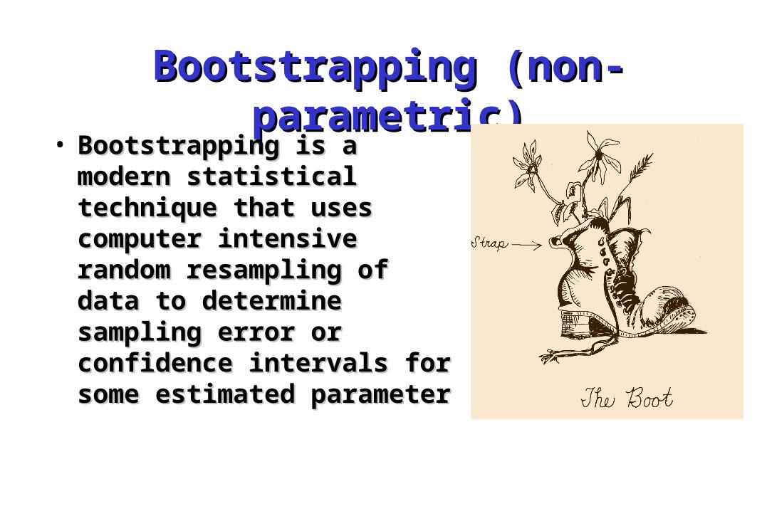
Bootstrapping (non-Bootstrapping (non-parametric)parametric)
• Bootstrapping is a modern Bootstrapping is a modern statistical technique that statistical technique that uses computer intensive uses computer intensive random resampling of data random resampling of data to determine sampling to determine sampling error or confidence error or confidence intervals for some intervals for some estimated parameterestimated parameter
BootstrappingBootstrapping• Characters are resampled with replacement Characters are resampled with replacement
to create many bootstrap replicate data setsto create many bootstrap replicate data sets• Each bootstrap replicate data set is analysed Each bootstrap replicate data set is analysed
(e.g. with parsimony, distance, ML)(e.g. with parsimony, distance, ML)• Agreement among the resulting trees is Agreement among the resulting trees is
summarized with a majority-rule consensus summarized with a majority-rule consensus treetree
• Frequency of occurrence of groups, bootstrap Frequency of occurrence of groups, bootstrap proportions (BPs), is a measure of support for proportions (BPs), is a measure of support for those groupsthose groups
• Additional information is given in partition Additional information is given in partition tablestables
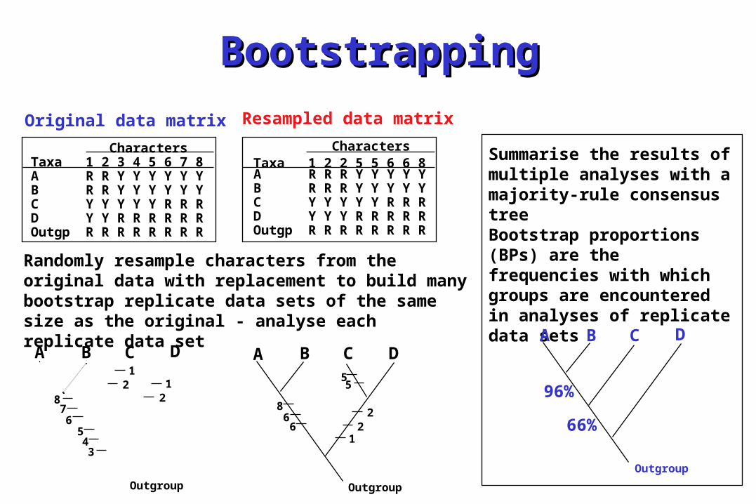
BootstrappingBootstrapping
Original data matrix
CharactersTaxa 1 2 3 4 5 6 7 8A R R Y Y Y Y Y YB R R Y Y Y Y Y YC Y Y Y Y Y R R RD Y Y R R R R R ROutgp R R R R R R R R
A B C D12 1
2
345
678
A B C D
122
55
668
Outgroup Outgroup
Resampled data matrix
CharactersTaxa 1 2 2 5 5 6 6 8A R R R Y Y Y Y YB R R R Y Y Y Y YC Y Y Y Y Y R R RD Y Y Y R R R R ROutgp R R R R R R R R
Randomly resample characters from the original data with replacement to build many bootstrap replicate data sets of the same size as the original - analyse each replicate data set
Summarise the results of multiple analyses with a majority-rule consensus treeBootstrap proportions (BPs) are the frequencies with which groups are encountered in analyses of replicate data sets
A B C D
Outgroup
96%
66%
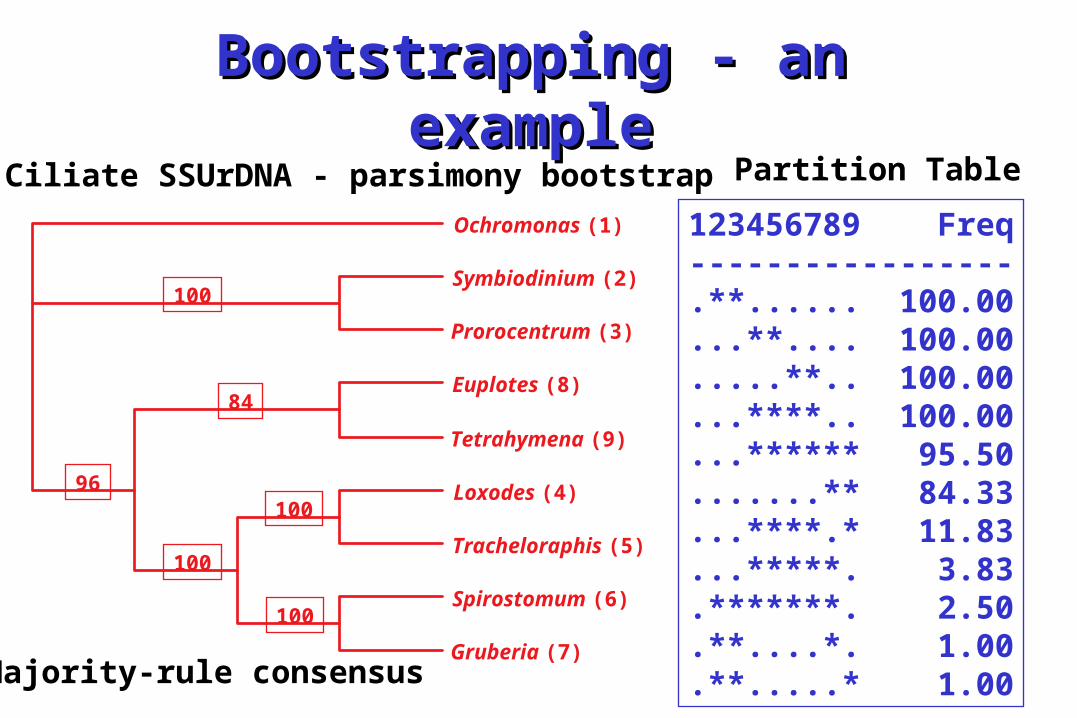
Bootstrapping - an Bootstrapping - an exampleexample
Ciliate SSUrDNA - parsimony bootstrap
123456789 Freq-----------------.**...... 100.00...**.... 100.00.....**.. 100.00...****.. 100.00...****** 95.50.......** 84.33...****.* 11.83...*****. 3.83.*******. 2.50.**....*. 1.00.**.....* 1.00Majority-rule consensus
Partition Table
Ochromonas (1)
Symbiodinium (2)
Prorocentrum (3)
Euplotes (8)
Tetrahymena (9)
Loxodes (4)
Tracheloraphis (5)
Spirostomum (6)
Gruberia (7)
100
96
84
100
100
100
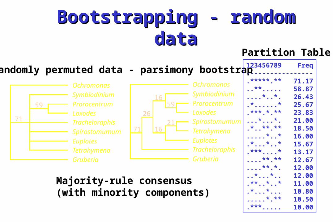
Bootstrapping - random Bootstrapping - random datadata
Randomly permuted data - parsimony bootstrap
Majority-rule consensus (with minority components)
Partition Table123456789 Freq-----------------.*****.** 71.17..**..... 58.87....*..*. 26.43.*......* 25.67.***.*.** 23.83...*...*. 21.00.*..**.** 18.50.....*..* 16.00.*...*..* 15.67.***....* 13.17....**.** 12.67....**.*. 12.00..*...*.. 12.00.**..*..* 11.00.*...*... 10.80.....*.** 10.50.***..... 10.00
Ochromonas
Symbiodinium
ProrocentrumLoxodesSpirostomumum
Tetrahymena
EuplotesTracheloraphis
Gruberia
71
26
1659
1621
Ochromonas
Symbiodinium
ProrocentrumLoxodesTracheloraphis
Spirostomumum
EuplotesTetrahymena
Gruberia
71
59
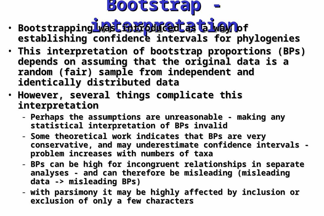
Bootstrap - Bootstrap - interpretationinterpretation• Bootstrapping was introduced as a way of Bootstrapping was introduced as a way of
establishing confidence intervals for phylogenies establishing confidence intervals for phylogenies • This interpretation of bootstrap proportions (BPs) This interpretation of bootstrap proportions (BPs)
depends on assuming that the original data is a depends on assuming that the original data is a random (fair) sample from independent and random (fair) sample from independent and identically distributed dataidentically distributed data
• However, several things complicate this However, several things complicate this interpretationinterpretation- Perhaps the assumptions are unreasonable - making any Perhaps the assumptions are unreasonable - making any
statistical interpretation of BPs invalidstatistical interpretation of BPs invalid- Some theoretical work indicates that BPs are very Some theoretical work indicates that BPs are very
conservative, and may underestimate confidence intervals - conservative, and may underestimate confidence intervals - problem increases with numbers of taxaproblem increases with numbers of taxa
- BPs can be high for incongruent relationships in separate BPs can be high for incongruent relationships in separate analyses - and can therefore be misleading (misleading data -analyses - and can therefore be misleading (misleading data -> misleading BPs)> misleading BPs)
- with parsimony it may be highly affected by inclusion or with parsimony it may be highly affected by inclusion or exclusion of only a few charactersexclusion of only a few characters
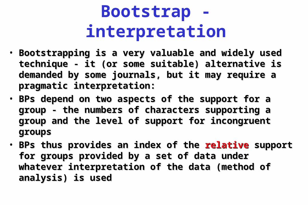
• Bootstrapping is a very valuable and widely used Bootstrapping is a very valuable and widely used technique - it (or some suitable) alternative is technique - it (or some suitable) alternative is demanded by some journals, but it may require a demanded by some journals, but it may require a pragmatic interpretation:pragmatic interpretation:
• BPs depend on two aspects of the support for a BPs depend on two aspects of the support for a group - the numbers of characters supporting a group - the numbers of characters supporting a group and the level of support for incongruent group and the level of support for incongruent groupsgroups
• BPs thus provides an index of the BPs thus provides an index of the relativerelative support support for groups provided by a set of data under whatever for groups provided by a set of data under whatever interpretation of the data (method of analysis) is interpretation of the data (method of analysis) is usedused
Bootstrap - interpretation
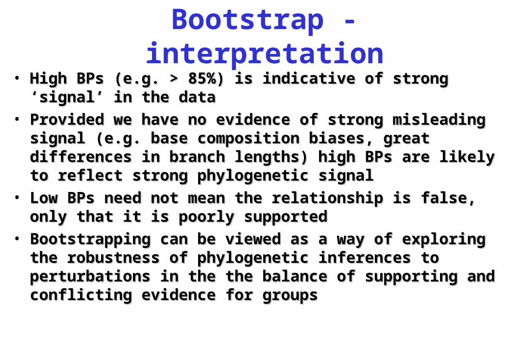
• High BPs (e.g. > 85%) is indicative of strong ‘signal’ High BPs (e.g. > 85%) is indicative of strong ‘signal’ in the datain the data
• Provided we have no evidence of strong misleading Provided we have no evidence of strong misleading signal (e.g. base composition biases, great signal (e.g. base composition biases, great differences in branch lengths) high BPs are likely to differences in branch lengths) high BPs are likely to reflect strong phylogenetic signalreflect strong phylogenetic signal
• Low BPs need not mean the relationship is false, Low BPs need not mean the relationship is false, only that it is poorly supportedonly that it is poorly supported
• Bootstrapping can be viewed as a way of exploring Bootstrapping can be viewed as a way of exploring the robustness of phylogenetic inferences to the robustness of phylogenetic inferences to perturbations in the the balance of supporting and perturbations in the the balance of supporting and conflicting evidence for groupsconflicting evidence for groups
Bootstrap - interpretation
JackknifingJackknifing
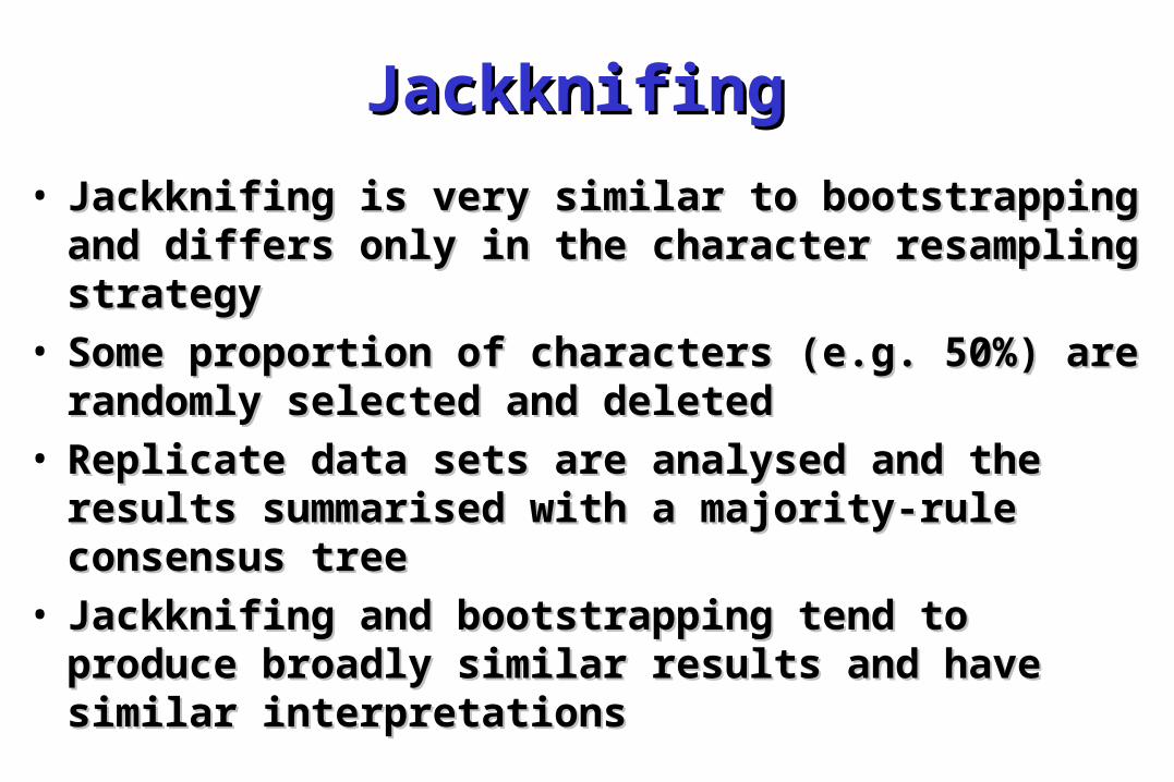
• Jackknifing is very similar to bootstrapping Jackknifing is very similar to bootstrapping and differs only in the character resampling and differs only in the character resampling strategystrategy
• Some proportion of characters (e.g. 50%) are Some proportion of characters (e.g. 50%) are randomly selected and deletedrandomly selected and deleted
• Replicate data sets are analysed and the Replicate data sets are analysed and the results summarised with a majority-rule results summarised with a majority-rule consensus treeconsensus tree
• Jackknifing and bootstrapping tend to produce Jackknifing and bootstrapping tend to produce broadly similar results and have similar broadly similar results and have similar interpretationsinterpretations
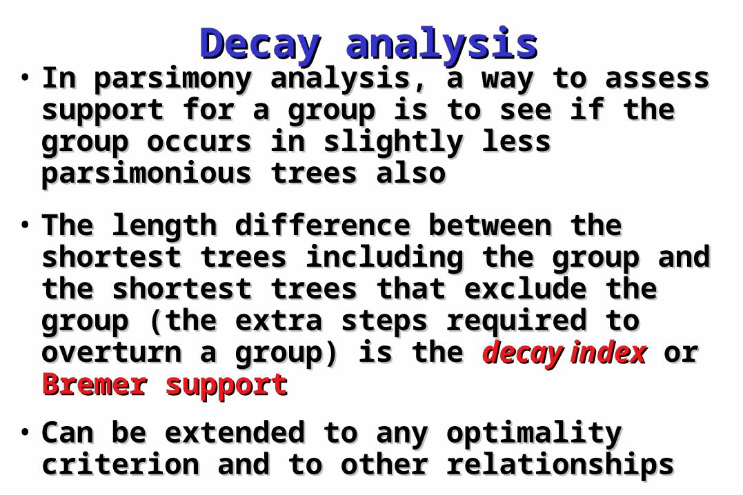
Decay analysisDecay analysis• In parsimony analysis, a way to assess In parsimony analysis, a way to assess
support for a group is to see if the group support for a group is to see if the group occurs in slightly less parsimonious trees occurs in slightly less parsimonious trees alsoalso
• The length difference between the The length difference between the shortest trees including the group and shortest trees including the group and the shortest trees that exclude the the shortest trees that exclude the group (the extra steps required to group (the extra steps required to overturn a group) is the overturn a group) is the decay indexdecay index or or Bremer supportBremer support
• Can be extended to any optimality Can be extended to any optimality criterion and to other relationshipscriterion and to other relationships
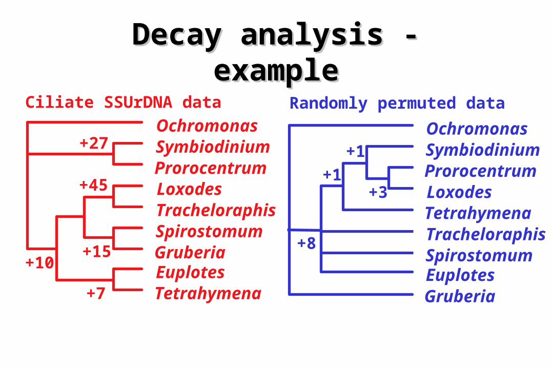
Decay analysis -Decay analysis -exampleexample
OchromonasSymbiodiniumProrocentrumLoxodesTracheloraphisSpirostomumGruberiaEuplotesTetrahymena
OchromonasSymbiodiniumProrocentrumLoxodesTetrahymenaTracheloraphisSpirostomumEuplotesGruberia
Ciliate SSUrDNA data Randomly permuted data
+27
+15 +8
+3
+1+1
+45
+7
+10
Decay analyses - in Decay analyses - in practicepractice
• Decay indices for each clade can be determined Decay indices for each clade can be determined by:by:
- Saving increasingly less parsimonious trees and Saving increasingly less parsimonious trees and producing corresponding strict consensus trees producing corresponding strict consensus trees until the consensus is completely unresolveduntil the consensus is completely unresolved
- analyses using reverse topological constraints analyses using reverse topological constraints to determine shortest trees that lack each cladeto determine shortest trees that lack each clade
- with the Autodecay or TreeRot programs (in with the Autodecay or TreeRot programs (in conjunction with PAUP)conjunction with PAUP)
Decay indices - Decay indices - interpretationinterpretation
• Generally, the higher the decay index the Generally, the higher the decay index the better the relative support for a groupbetter the relative support for a group
• Like BPs, decay indices may be misleading if Like BPs, decay indices may be misleading if the data is misleadingthe data is misleading
• Unlike BPs decay indices are not scaled (0-Unlike BPs decay indices are not scaled (0-100) and it is less clear what is an acceptable 100) and it is less clear what is an acceptable decay indexdecay index
• Magnitude of decay indices and BPs generally Magnitude of decay indices and BPs generally correlated (i.e. they tend to agree)correlated (i.e. they tend to agree)
• Only groups found in all most parsimonious Only groups found in all most parsimonious trees have decay indices > zerotrees have decay indices > zero
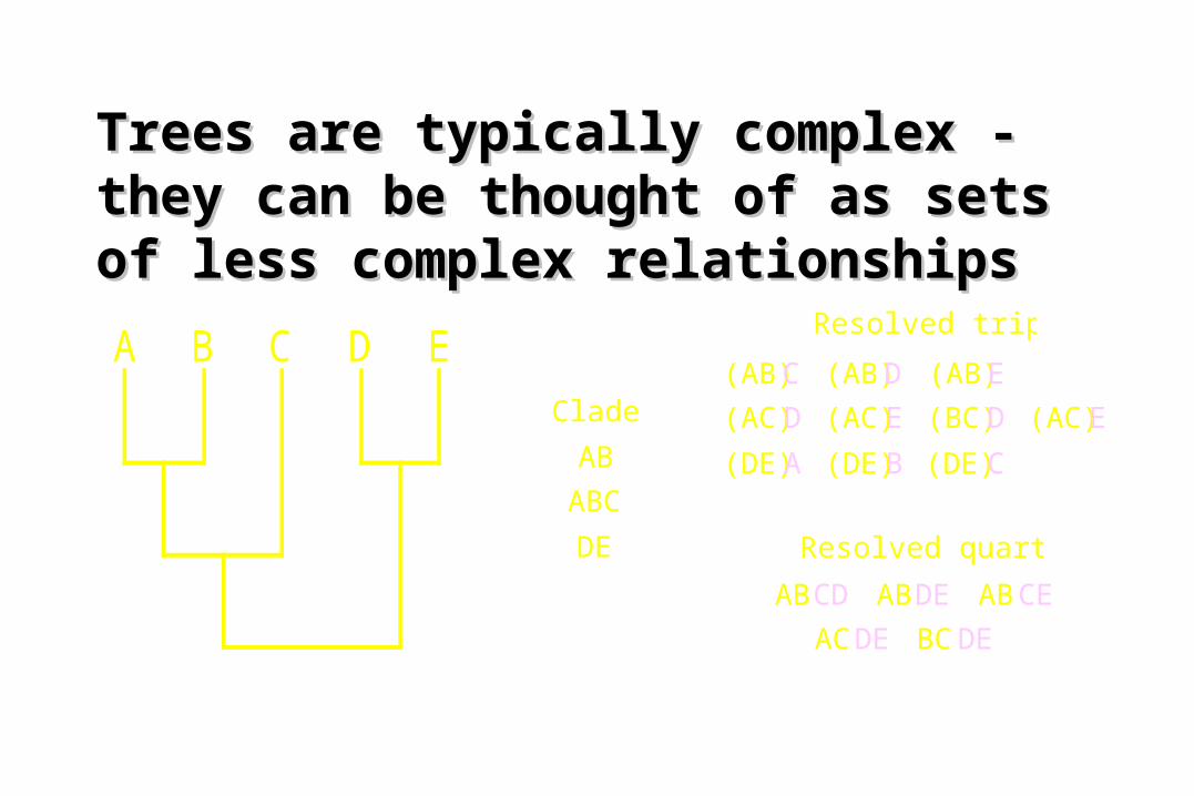
Trees are typically complex - Trees are typically complex - they can be thought of as sets of they can be thought of as sets of less complex relationshipsless complex relationships
A B C D E(AB)C
(AC)D
(DE)A
(AB)D
(AC)E
(DE)B
(AB)E
(BC)D
(DE)C
(AC)E
Resolved triplets
ABCD
ACDE
ABDE
BCDE
ABCE
Resolved quartets
Clades
AB
ABC
DE
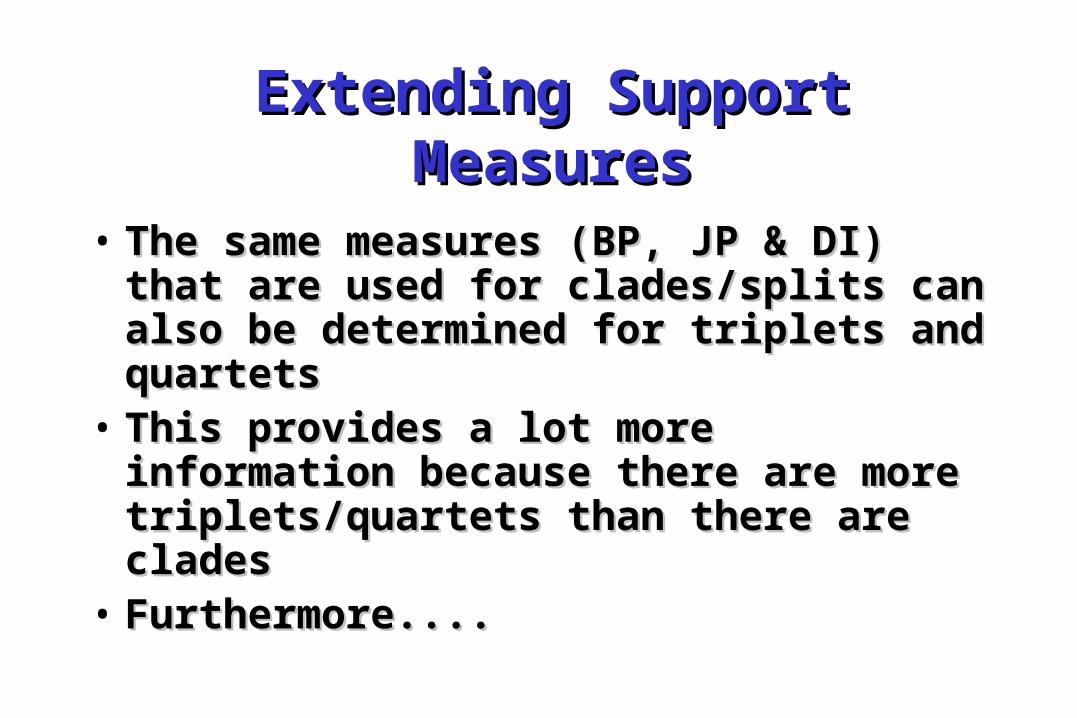
Extending Support Extending Support MeasuresMeasures
• The same measures (BP, JP & DI) The same measures (BP, JP & DI) that are used for clades/splits can that are used for clades/splits can also be determined for triplets and also be determined for triplets and quartetsquartets
• This provides a lot more This provides a lot more information because there are information because there are more triplets/quartets than there more triplets/quartets than there are cladesare clades
• Furthermore....Furthermore....
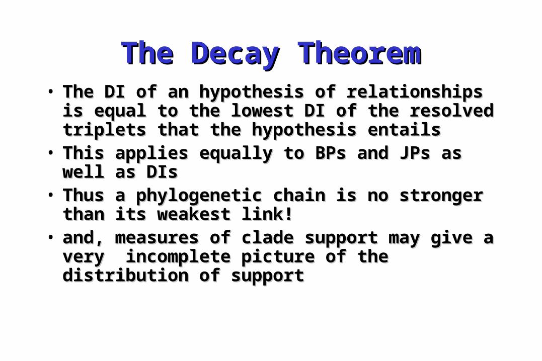
The Decay TheoremThe Decay Theorem• The DI of an hypothesis of relationships The DI of an hypothesis of relationships
is equal to the lowest DI of the resolved is equal to the lowest DI of the resolved triplets that the hypothesis entailstriplets that the hypothesis entails
• This applies equally to BPs and JPs as This applies equally to BPs and JPs as well as DIswell as DIs
• Thus a phylogenetic chain is no stronger Thus a phylogenetic chain is no stronger than its weakest link!than its weakest link!
• and, measures of clade support may and, measures of clade support may give a very incomplete picture of the give a very incomplete picture of the distribution of supportdistribution of support
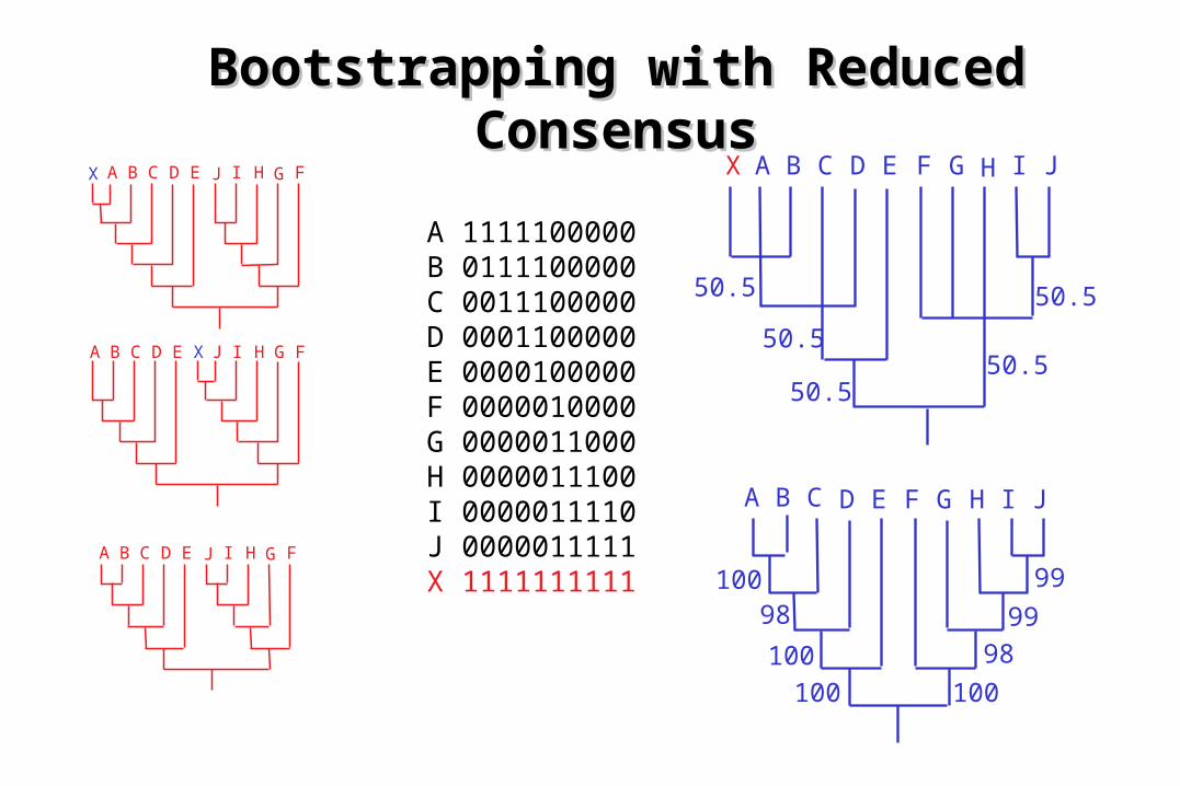
Bootstrapping with Reduced Bootstrapping with Reduced ConsensusConsensus
A B C D E FGHIJ
A B C D E FGHIJ
X
A B C D E FGHIJX
A B C D E F G H I J
A B C D E F G H I J
X
50.5
50.5
50.550.5
50.5
100
100 100
100
99
99
98
98
A 1111100000B 0111100000C 0011100000D 0001100000E 0000100000F 0000010000G 0000011000H 0000011100I 0000011110J 0000011111X 1111111111
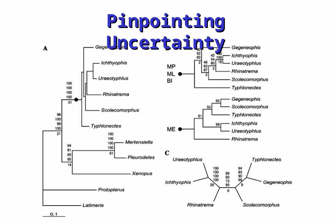
Pinpointing UncertaintyPinpointing Uncertainty
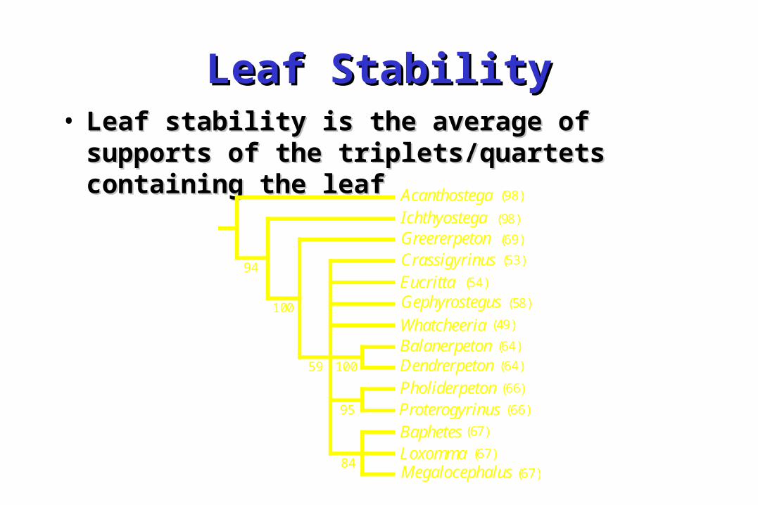
Leaf StabilityLeaf Stability• Leaf stability is the average of supports Leaf stability is the average of supports
of the triplets/quartets containing the of the triplets/quartets containing the leafleaf Acanthostega
IchthyostegaGreererpetonCrassigyrinusEucritta
Whatcheeria
Gephyrostegus
BalanerpetonDendrerpeton
ProterogyrinusPholiderpeton
MegalocephalusLoxommaBaphetes
94
100
59
84
(98)
(98)
(69)
(53)
(54)
(58)
(49)
(64)
(64)
(66)
(66)
(67)
(67)
(67)
100
95
PTP tests of groupsPTP tests of groups• A number of randomization tests have been A number of randomization tests have been
proposed for evaluating particular groups proposed for evaluating particular groups rather than entire data matrices by testing null rather than entire data matrices by testing null hypotheses regarding the level of support they hypotheses regarding the level of support they receive from the datareceive from the data
• Randomisation can be of the data or the groupRandomisation can be of the data or the group• These methods have not become widely used These methods have not become widely used
both because they are not readily performed both because they are not readily performed and because their properties are still under and because their properties are still under investigationinvestigation
• One type, the topology dependent PTP tests are One type, the topology dependent PTP tests are included in PAUP* but have serious problemsincluded in PAUP* but have serious problems
Comparing competing Comparing competing phylogenetic hypothesesphylogenetic hypotheses - tests - tests
of two of two (or more)(or more) trees trees• Particularly useful techniques are those Particularly useful techniques are those
designed to allow evaluation of alternative designed to allow evaluation of alternative phylogenetic hypothesesphylogenetic hypotheses
• Several such tests allow us to determine if Several such tests allow us to determine if one tree is statistically significantly worse one tree is statistically significantly worse than another:than another:
Winning sites, Templeton, Kishino-Hasegawa, Winning sites, Templeton, Kishino-Hasegawa, parametric bootstrapping (SOWH)parametric bootstrapping (SOWH)
Shimodaira-Hasegawa, Approximately Unbiased Shimodaira-Hasegawa, Approximately Unbiased
• Tests are of the null hypothesis that the Tests are of the null hypothesis that the differences between two trees (A and B) are differences between two trees (A and B) are no greater than expected from sampling errorno greater than expected from sampling error
• The simplest ‘wining sites’ test sums the The simplest ‘wining sites’ test sums the number of sites supporting tree A over tree B number of sites supporting tree A over tree B and vice versa (those having fewer steps on, and vice versa (those having fewer steps on, and better fit to, one of the trees)and better fit to, one of the trees)
• Under the null hypothesis characters are Under the null hypothesis characters are equally likely to support tree A or tree B and a equally likely to support tree A or tree B and a binomial distribution gives the probability of binomial distribution gives the probability of the observed difference in numbers of winning the observed difference in numbers of winning sitessites
Tests of two trees
The Templeton testThe Templeton test
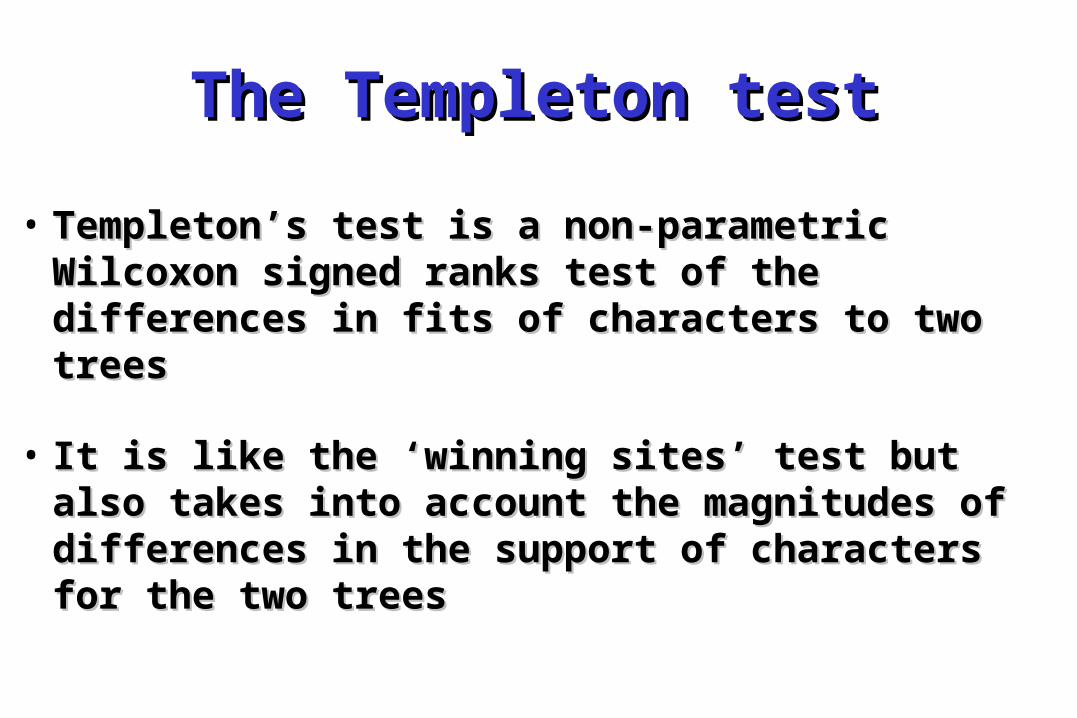
• Templeton’s test is a non-parametric Templeton’s test is a non-parametric Wilcoxon signed ranks test of the Wilcoxon signed ranks test of the differences in fits of characters to two differences in fits of characters to two treestrees
• It is like the ‘winning sites’ test but also It is like the ‘winning sites’ test but also takes into account the magnitudes of takes into account the magnitudes of differences in the support of characters differences in the support of characters for the two treesfor the two trees
Templeton’s test - an exampleTempleton’s test - an exampleS
eym
ou
ria
dae
Dia
dec
tom
orp
ha
Syn
apsi
da
Par
arep
tili
a
Cap
torh
inid
ae
Pal
eoth
yri
s
Cla
ud
iosa
uru
s
Yo
un
gin
ifo
rmes
Arc
ho
sau
rom
orp
ha
Lep
ido
sau
rifo
rmes
Pla
cod
us
Eo
sau
rop
tery
gia
Ara
eosc
elid
ia
2
1
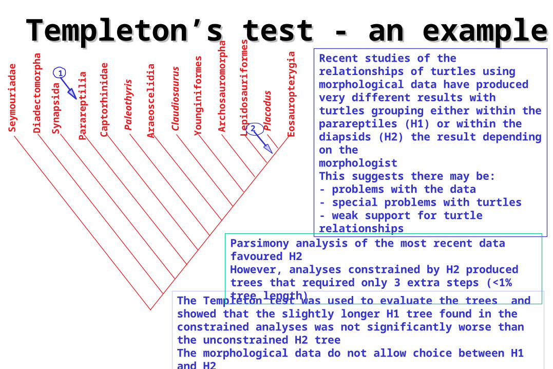
Recent studies of the relationships of turtles using morphological data have produced very different results with turtles grouping either within the parareptiles (H1) or within the diapsids (H2) the result depending on themorphologist This suggests there may be:- problems with the data- special problems with turtles- weak support for turtle relationships
The Templeton test was used to evaluate the trees and showed that the slightly longer H1 tree found in the constrained analyses was not significantly worse than the unconstrained H2 treeThe morphological data do not allow choice between H1 and H2
Parsimony analysis of the most recent data favoured H2However, analyses constrained by H2 produced trees that required only 3 extra steps (<1% tree length)
Kishino-Hasegawa testKishino-Hasegawa test• The Kishino-Hasegawa test is similar in using The Kishino-Hasegawa test is similar in using
differences in the support provided by differences in the support provided by individual sites for two trees to determine if individual sites for two trees to determine if the overall differences between the trees are the overall differences between the trees are significantly greater than expected from significantly greater than expected from random sampling errorrandom sampling error
• It is a parametric test that depends on It is a parametric test that depends on assumptions that the characters are assumptions that the characters are independent and identically distributed (the independent and identically distributed (the same assumptions underlying the statistical same assumptions underlying the statistical interpretation of bootstrapping)interpretation of bootstrapping)
• It can be used with parsimony and maximum It can be used with parsimony and maximum likelihood - implemented in PHYLIP and likelihood - implemented in PHYLIP and PAUP*PAUP*
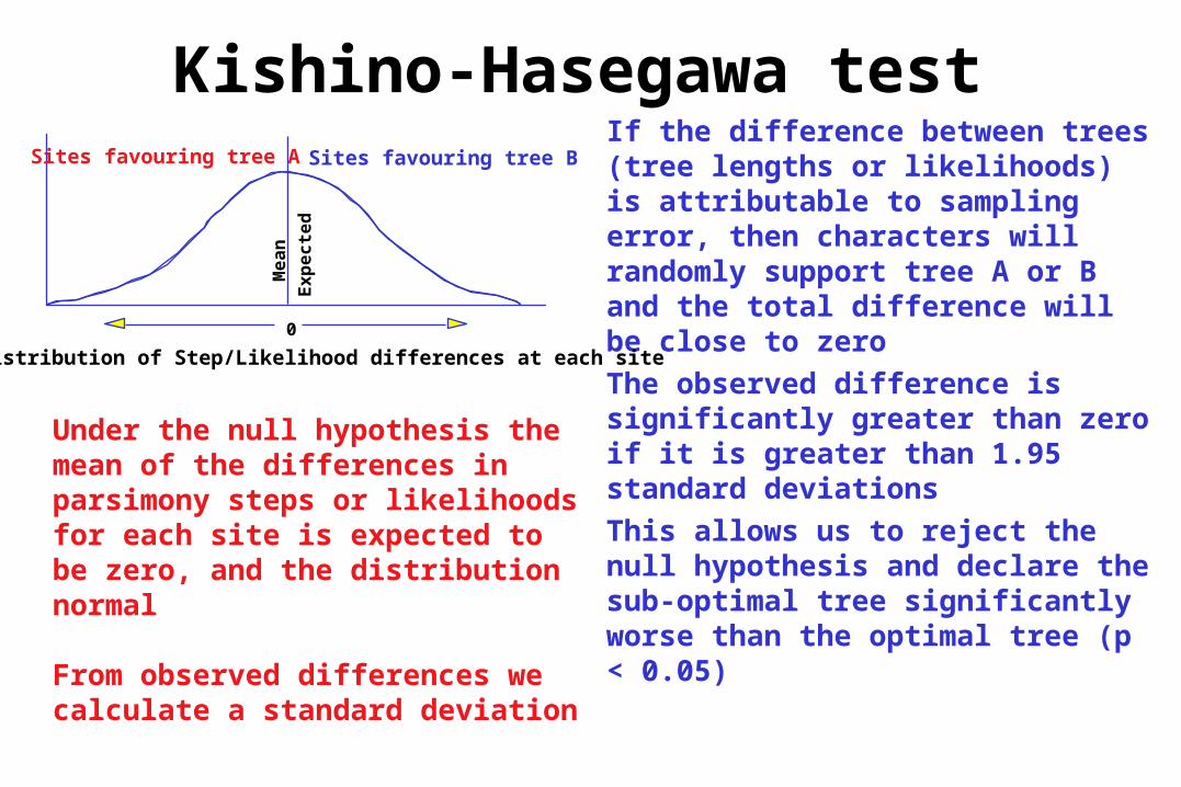
Kishino-Hasegawa testIf the difference between trees (tree lengths or likelihoods) is attributable to sampling error, then characters will randomly support tree A or B and the total difference will be close to zeroThe observed difference is significantly greater than zero if it is greater than 1.95 standard deviations This allows us to reject the null hypothesis and declare the sub-optimal tree significantly worse than the optimal tree (p < 0.05)
Under the null hypothesis the mean of the differences in parsimony steps or likelihoods for each site is expected to be zero, and the distribution normal
From observed differences we calculate a standard deviation
Distribution of Step/Likelihood differences at each site
0
Sites favouring tree A Sites favouring tree B
Ex
pe
cte
d
M
ea
n
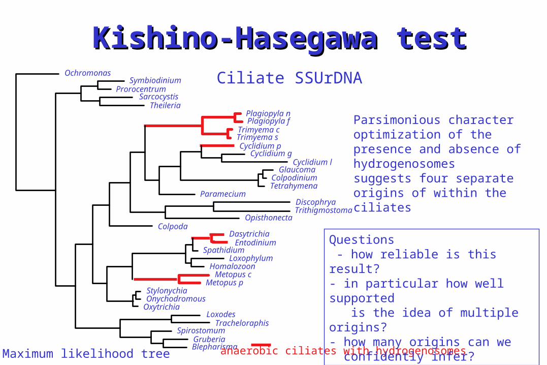
Kishino-Hasegawa testKishino-Hasegawa testCiliate SSUrDNA
Maximum likelihood tree
OchromonasSymbiodinium
ProrocentrumSarcocystis
TheileriaPlagiopyla nPlagiopyla f
Trimyema cTrimyema sCyclidium p
Cyclidium gCyclidium l
GlaucomaColpodiniumTetrahymena
ParameciumDiscophryaTrithigmostoma
OpisthonectaColpoda
DasytrichiaEntodinium
SpathidiumLoxophylum
HomalozoonMetopus c
Metopus pStylonychiaOnychodromous
OxytrichiaLoxodes
TracheloraphisSpirostomum
GruberiaBlepharismaanaerobic ciliates with hydrogenosomes
Parsimonious character optimization of the presence and absence of hydrogenosomes suggests four separate origins of within the ciliates
Questions - how reliable is this result?- in particular how well supported is the idea of multiple origins?- how many origins can we confidently infer?
Kishino-Hasegawa testKishino-Hasegawa testOchromonasSymbiodiniumProrocentrumSarcocystisTheileriaPlagiopyla nPlagiopyla fTrimyema cTrimyema sCyclidium pCyclidium gCyclidium lDasytrichiaEntodiniumLoxophylumHomalozoonSpathidiumMetopus cMetopus pLoxodesTracheloraphisSpirostomumGruberiaBlepharismaDiscophryaTrithigmostomaStylonychiaOnychodromousOxytrichiaColpodaParameciumGlaucomaColpodiniumTetrahymenaOpisthonecta
OchromonasSymbiodiniumProrocentrumSarcocystisTheileriaPlagiopyla nPlagiopyla fTrimyema cTrimyema sCyclidium p
Cyclidium gCyclidium l
HomalozoonSpathidium
DasytrichiaEntodinium
Loxophylum
Metopus cMetopus p
LoxodesTracheloraphisSpirostomumGruberiaBlepharismaDiscophryaTrithigmostomaStylonychiaOnychodromousOxytrichiaColpodaParameciumGlaucomaColpodiniumTetrahymenaOpisthonecta
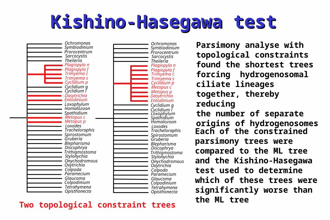
Parsimony analyse with topological constraints found the shortest trees forcing hydrogenosomal ciliate lineages together, thereby reducingthe number of separate origins of hydrogenosomes
Two topological constraint trees
Each of the constrained parsimony trees were compared to the ML tree and the Kishino-Hasegawa test used to determine which of these trees were significantly worse than the ML tree
Kishino-Hasegawa testKishino-Hasegawa test
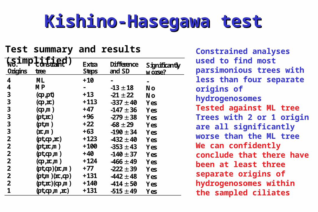
No. Constraint Extra Difference SignificantlyOrigins tree Steps and SD worse?4 ML +10 - -4 MP - -13 18 No3 (cp,pt) +13 -21 22 No3 (cp,rc) +113 -337 40 Yes3 (cp,m) +47 -147 36 Yes3 (pt,rc) +96 -279 38 Yes3 (pt,m) +22 -68 29 Yes3 (rc,m) +63 -190 34 Yes2 (pt,cp,rc) +123 -432 40 Yes2 (pt,rc,m) +100 -353 43 Yes2 (pt,cp,m) +40 -140 37 Yes2 (cp,rc,m) +124 -466 49 Yes2 (pt,cp)(rc,m) +77 -222 39 Yes2 (pt,m)(rc,cp) +131 -442 48 Yes2 (pt,rc)(cp,m) +140 -414 50 Yes1 (pt,cp,m,rc) +131 -515 49 Yes
Constrained analyses used to find most parsimonious trees with less than four separate origins of hydrogenosomesTested against ML treeTrees with 2 or 1 origin are all significantly worse than the ML treeWe can confidently conclude that there have been at least three separate origins of hydrogenosomes within the sampled ciliates
Test summary and results (simplified)
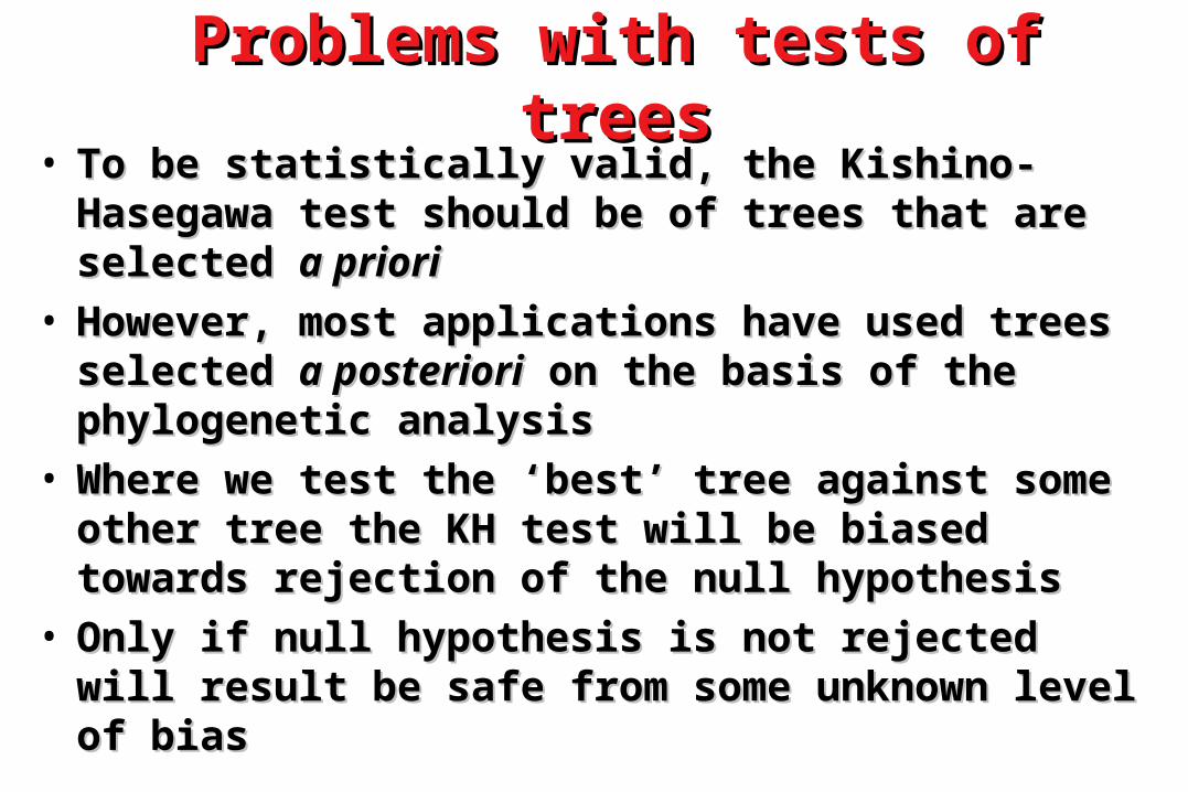
Problems with tests of treesProblems with tests of trees• To be statistically valid, the Kishino-To be statistically valid, the Kishino-
Hasegawa test should be of trees that are Hasegawa test should be of trees that are selected selected a prioria priori
• However, most applications have used trees However, most applications have used trees selected selected a posterioria posteriori on the basis of the on the basis of the phylogenetic analysisphylogenetic analysis
• Where we test the ‘best’ tree against some Where we test the ‘best’ tree against some other tree the KH test will be biased towards other tree the KH test will be biased towards rejection of the null hypothesisrejection of the null hypothesis
• Only if null hypothesis is not rejected will Only if null hypothesis is not rejected will result be safe from some unknown level of result be safe from some unknown level of biasbias
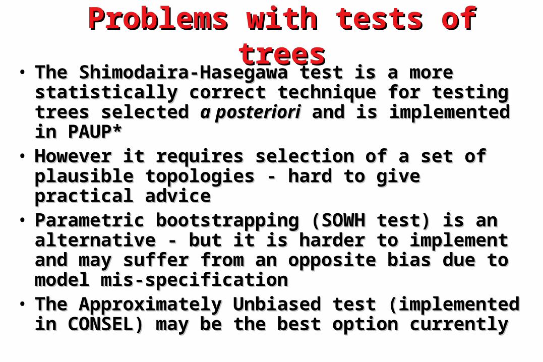
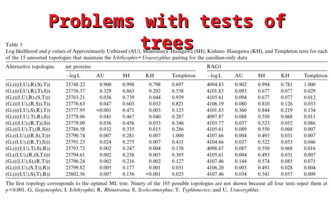
Problems with tests of treesProblems with tests of trees• The Shimodaira-Hasegawa test is a more The Shimodaira-Hasegawa test is a more
statistically correct technique for testing statistically correct technique for testing trees selected trees selected a posterioria posteriori and is and is implemented in PAUP*implemented in PAUP*
• However it requires selection of a set of However it requires selection of a set of plausible topologies - hard to give practical plausible topologies - hard to give practical adviceadvice
• Parametric bootstrapping (SOWH test) is an Parametric bootstrapping (SOWH test) is an alternative - but it is harder to implement and alternative - but it is harder to implement and may suffer from an opposite bias due to may suffer from an opposite bias due to model mis-specificationmodel mis-specification
• The Approximately Unbiased test The Approximately Unbiased test (implemented in CONSEL) may be the best (implemented in CONSEL) may be the best option currentlyoption currently
Problems with tests of treesProblems with tests of trees
Taxonomic CongruenceTaxonomic Congruence• Trees inferred from different data sets Trees inferred from different data sets
(different genes, morphology) should (different genes, morphology) should agree if they are accurateagree if they are accurate
• Congruence between trees is best Congruence between trees is best explained by their accuracyexplained by their accuracy
• Congruence can be investigated using Congruence can be investigated using consensus (and supertree) methodsconsensus (and supertree) methods
• Incongruence requires further work to Incongruence requires further work to explain or resolve disagreements explain or resolve disagreements
Reliability of Phylogenetic Reliability of Phylogenetic MethodsMethods
• Phylogenetic methods (e.g. parsimony, Phylogenetic methods (e.g. parsimony, distance, ML) can also be evaluated in distance, ML) can also be evaluated in terms of their general performance, terms of their general performance, particularly their:particularly their:consistency - approach the truth with more consistency - approach the truth with more
datadata
efficiency - how quickly (how much data)efficiency - how quickly (how much data)
robustness - sensitivity to violations of robustness - sensitivity to violations of assumptionsassumptions
• Studies of these properties can be Studies of these properties can be analytical or by simulationanalytical or by simulation
Reliability of Phylogenetic Reliability of Phylogenetic MethodsMethods
• There have been many arguments that There have been many arguments that ML methods are best because they have ML methods are best because they have desirable statistical properties, such as desirable statistical properties, such as consistencyconsistency
• However, ML does not always have However, ML does not always have these propertiesthese properties– if the model is wrong/inadequate if the model is wrong/inadequate
(fortunately this is testable to some extent)(fortunately this is testable to some extent)– properties not yet demonstrated for properties not yet demonstrated for
complex inference problems such as complex inference problems such as phylogenetic treesphylogenetic trees
Reliability of Phylogenetic Reliability of Phylogenetic MethodsMethods
• ““Simulations show that ML methods generally Simulations show that ML methods generally outperform distance and parsimony methods outperform distance and parsimony methods over a broad range of realistic conditions”over a broad range of realistic conditions”
Whelan et al. 2001 Whelan et al. 2001 Trends in GeneticsTrends in Genetics 17:262-27217:262-272
• But…But…• Most simulations cover a narrow range of Most simulations cover a narrow range of
very (unrealistically) simple conditionsvery (unrealistically) simple conditions– few taxa (typically just four!)few taxa (typically just four!)– few parameters (standard models - JC, K2P few parameters (standard models - JC, K2P
etc)etc)
Reliability of Phylogenetic Reliability of Phylogenetic MethodsMethods• Simulations with four taxa have shown:Simulations with four taxa have shown:
- Model based methods - distance and Model based methods - distance and maximum likelihood perform well when the maximum likelihood perform well when the model is accurate (not surprising!)model is accurate (not surprising!)
- Violations of assumptions can lead to Violations of assumptions can lead to inconsistency for all methods (inconsistency for all methods (a Felsenstein a Felsenstein zonezone) when branch lengths or rates are highly ) when branch lengths or rates are highly unequalunequal
- Maximum likelihood methods are quite robust Maximum likelihood methods are quite robust to violations of model assumptionsto violations of model assumptions
- Weighting can improve the performance of Weighting can improve the performance of parsimony (reduce the size of the Felsenstein parsimony (reduce the size of the Felsenstein zone)zone)
Reliability of Phylogenetic Reliability of Phylogenetic MethodsMethods
• However:However:- Generalising from four taxon simulations may be Generalising from four taxon simulations may be
dangerous as conclusions may not hold for more dangerous as conclusions may not hold for more complex casescomplex cases
- A few large scale simulations (many taxa) have A few large scale simulations (many taxa) have suggested that parsimony can be very accurate and suggested that parsimony can be very accurate and efficientefficient
- Most methods are accurate in correctly recovering Most methods are accurate in correctly recovering known phylogenies produced in laboratory studies known phylogenies produced in laboratory studies
• More realistic simulations are needed if they More realistic simulations are needed if they are to help in choosing/understanding methodsare to help in choosing/understanding methods