Assessing impact of climate change on season length in

Assessing impact of climate change on season lengthin Karnataka for IPCC SRES scenarios

Aavudai Anandhi

CUNY Institute for Sustainable Cities/Hunter College, City University of New York,New York, United States of America.

Changes in seasons and season length are an indicator, as well as an effect, of climate change.Seasonal change profoundly affects the balance of life in ecosystems and impacts essential humanactivities such as agriculture and irrigation. This study investigates the uncertainty of season lengthin Karnataka state, India, due to the choice of scenarios, season type and number of seasons.Based on the type of season, the monthly sequences of variables (predictors) were selected fromdatasets of NCEP and Canadian General Circulation Model (CGCM3). Seasonal stratificationswere carried out on the selected predictors using K-means clustering technique. The results ofcluster analysis revealed increase in average, wet season length in A2, A1B and B1 scenariostowards the end of 21st century. The increase in season length was higher for A2 scenario whereasit was the least for B1 scenario. COMMIT scenario did not show any change in season length.However, no change in average warm and cold season length was observed across the four scenariosconsidered. The number of seasons was increased from 2 to 5. The results of the analysis revealedthat no distinct cluster could be obtained when the number of seasons was increased beyondthree.

1. Introduction

Changes in seasons and its length are an indicator,as well as an effect, of climate change. They reflectthe variations that are occurring in the cyclingof energy in the global environment and pro-foundly affect the balance of life in ecosystems,impact agriculture and water balance of a region.Hence, knowing the future changes in season lengthin developing countries like India helps policymakers and general public for realistic assessment,management and mitigation of natural disasters,and for sustainable development. However, thereis dearth of attempts in published literature thatstudies the variability in the future season lengthin this part of the world.

Global climate models (GCMs) are widely usedto simulate climate conditions on earth, severaldecades into the future, for each of the con-structed climate change scenarios. As GCMs are

generally run at coarser scale to cover the wholeGlobe, they are inefficient in simulating regionalclimatic conditions on earth. For this purpose,weather classification methods have been used inthe past to transfer the information on large-scalepatterns provided by GCMs (predictors) to seasons(predictand) at regional scales.

Owing to the availability of a number of GCMs,climate change scenarios, classification methods,predictors, definitions of seasons, number of sea-sons, etc., prediction of season length is subject toa number of uncertainties. Hence, there is a needto study the changes in season length of a regionby the various alternatives available.

The objective of this study is to investigatethe variability of future season length to some ofthe uncertainties such as the choice of climatescenario, predictors, definition of seasons. Thechosen methodology is tested for the Karnatakastate in India.

Keywords. General circulation model (GCM); third generation Canadian coupled global climate model (CGCM3); SRESA1B, A2, B1 and COMMIT scenarios; K-means clustering; uncertainty.

J. Earth Syst. Sci. 119, No. 4, August 2010, pp. 447–460© Indian Academy of Sciences 447

448 Aavudai Anandhi

2. Background

In order to obtain season length, the seasonsare to be defined. In general, depending on theapplication, seasons are defined in a number ofways, such as astronomical seasons, meteorologi-cal seasons (e.g., Argiriou et al 2004) and standardseasons (Tuller 1990). In this study seasons aredivided based on meteorological variables (namely,rainfall, temperature and wind), as they affectagriculture and irrigation of the region and alsothey are commonly used in climate change impactstudies.

A number of studies have analyzed the rain-fall and temperatures simulated by the IPCC AR4GCMs and regional climate model (RCM) fordifferent regions of India (Rupa Kumar et al 2006;Kripalini et al 2007; Yadav et al 2010a). Thesestudies show an increase in mean monsoon rainfalland temperature towards the end of 21st centuryunder scenarios of increasing greenhouse gas con-centrations and sulphate aerosols. Though a num-ber of studies have analyzed the changes in rainfalland temperatures for the different seasons in India,there is a lacuna in research to study the changesin season length for the future scenarios.

The season length may be defined as conven-tional (fixed) length or ‘floating’ length. In a fixedseason length, the starting dates and length ofseasons remain the same for every year. In con-trast, in a ‘floating’ season length, the date of onsetand duration of each season is allowed to changefrom year to year. Studies have shown that floatingseasons reflect ‘natural’ seasons contained in theclimate data better than fixed seasons, especiallyunder changing climate conditions (Winkler et al1997; Anandhi et al 2008). Therefore, in this study,floating season length is used to effectively capturethe changes in the future climate conditions.

The weather classification methods are used inthis study to define floating meteorologicalseason length, link large-scale circulation patternand surface weather by grouping the daily/monthly datasets of large-scale circulation orsurface climate variables into a finite number ofdiscrete weather types or ‘seasons’. The classifi-cation may be subjective (e.g., Lamb 1972),objective (e.g., Tripathi et al 2006), or hybrid(e.g., Sailor et al 2008). In subjective classifica-tion, the stratifications were carried out manuallyusing empirical rules where the meteorologi-cal scientist’s experience is applied and reflectthe knowledge of meteorologists. These stratifica-tions cannot be easily replicated and are labour-intensive. In objective classification methods, avariety of automated techniques were developedusing computers to group the seasons, and thereis subjectivity in the choice of the algorithm.

Hybrid techniques combine elements of empiricaland automated procedures for grouping seasons,thereby avoiding time delay and enabling the pro-duction of easily reproducible and interpretableresults. In this study the hybrid approach usingK-means clustering (MacQueen 1967) was usedsince it had the advantages of both subjective andobjective approaches.

In this study, season length is proposed to beinvestigated for:

• each of the four scenarios specified inSpecial Report on Emission Scenarios (SRES;Nakicenovic et al 2000) that are relevant toIPCC’s fourth assessment report (AR4) (Alleyet al 2007) namely A1B, A2, B1 and COMMIT,

• the seasons defined based on the three meteoro-logical variables,

• the predictors used in the classification of sea-sons, and

• varying number of seasons.

3. Study region and data used

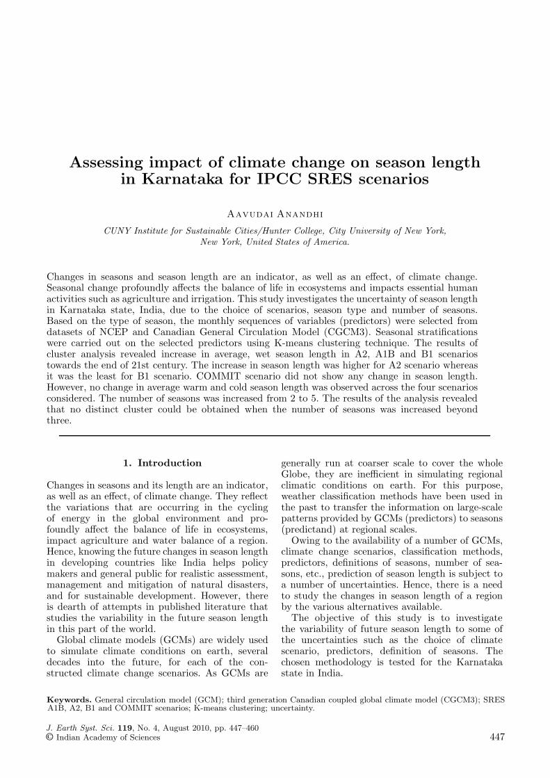
The chosen methodology is tested for theKarnataka state of India (figure 1). It has an areaof 191791 km2 situated between 11◦N to 18◦N lati-tudes and 74◦E and 78◦E longitudes. The state hasthe second largest arid and semi-arid regions in thecountry after Rajasthan.

The predictors used for this study comprise ofthe reanalysis data extracted from database pre-pared by National Centers for Environmental Pre-diction (NCEP) (Kalnay et al 1996), and the dataextracted from simulations by Canadian Centerfor Climate Modeling and Analysis’s (CCCma)third generation Coupled Global Climate Model(CGCM3). The details of the data used are fur-nished in table 1. A brief description of the fourfuture scenarios is provided in table 2. The pre-dictors at each of the nine NCEP grid points andtwelve CGCM3 grid points which are within andsurrounding the study region are used in the study.The list of predictors and their description usedare provided in table 3. In addition to the pre-dictors, the surface average temperature and rain-fall were also extracted from NCEP and CGCM3database. The GCM data and the informationon atmospheric flux are re-gridded to a common2.5◦ NCEP grid using Grid Analysis and DisplaySystem (GrADS) (Doty and Kinter 1993).

4. Methodology

The methodology adopted for stratification intoseasons is presented in the form of a flowchart

Impact of climate change on season length in Karnataka for IPCC SRES scenarios 449

Figure 1. Location of Karnataka state of India. The latitude, longitude and scale of the map refer to the Karnataka state.The data extracted from GCMs are re-gridded to the nine 2.5◦ NCEP grid points. Among the nine grid points 1, 4 and 7are over Arabian Sea, and the remaining points are on land.

Table 1. Details of meteorological data used in the study.

Data type Source of data Period Details Time scale

CGCM3 T/47 data onatmospheric variables

http://www.cccma.bc.ec.gc.ca/cgi-bin/data/cgcm3

1948–2100baseline: 20C3M –

1948 to 2000.future: SRES A1B,A2, B1 and COMMIT– 2001 to 2100

12 grid points foratmospheric variables,with grid box ≈3.75◦.

Latitudes range:9.28◦N–20.41◦N.

Longitudes range:71.25◦E–78.75◦E.

Monthly

NCEP re-analysis dataof atmosphericvariables

Kalnay et al (1996) 1948–2000 9 grid points foratmospheric variableswith grid box 2.5◦.

Latitudes range:12.5◦N–17.5◦N.

Longitudes range:72.5◦E–77.5◦E.

Monthly

Observed historicalrainfall for Karnataka

High-resolutiongridded daily rainfalldata (Rajeevan et al2005, 2006)

1951–2001 20 grid points with gridbox 1◦ in Karnataka areconsidered.

Monthly

(figure 2). The steps involved in the stratificationinto seasons are as follows:

Step 1. Selection of appropriate predictors fromregridded NCEP and GCM monthly datasets asprobable predictors at each of the NCEP gridpoints within and surrounding the study region(figure 1).

Step 2. Preparation of scatter plots and corre-lation plots using three measures of dependence

(Pearson’s product moment correlation and non-parametric rank correlations namely Spearman’srho and Kendall’s tau explained in Annexure)between predictor variables in NCEP and GCMdatasets after removing significant autocorrelationsand trends. Then, examine the correlation betweenpredictors in NCEP and GCM datasets.

Step 3. Selection of highly correlated predictors(potential predictors) with reference to a speci-fied threshold Tng for correlation between predictor

450 Aavudai Anandhi

Table 2. Explanation of the scenarios considered in the study.

Dataset Description Duration

Climate of the 20thCentury (20C3M)

Atmospheric CO2 concentrations and other inputdata are based on historical records or esti-mates beginning around the time of the Indus-trial Revolution.

1870–2000

Year 2000 equivalentCO2 (COMMIT)

Atmospheric CO2 concentrations are held atyear 2000 levels. This experiment is based onconditions that already exist (e.g., ‘committed’climate change).

2001–2100

SRES B1 (550 ppmequivalent CO2)

Atmospheric CO2 concentrations reach 550 ppmin the year 2100 in a world characterized bylow population growth, high GDP growth, lowenergy use, high land-use changes, low resourceavailability and medium introduction of new andefficient technologies.

2001–2100

SRES A1B (720 ppmequivalent CO2)

Atmospheric CO2 concentrations reach 720 ppmin the year 2100 in a world characterized by lowpopulation growth, very high GDP growth, veryhigh energy use, low land-use changes, mediumresource availability and rapid introduction ofnew and efficient technologies.

2001–2100

SRES A2 (850 ppmequivalent CO2)

Atmospheric CO2 concentrations reach 850 ppmin the year 2100 in a world characterized byhigh population growth, medium GDP growth,high energy use, medium/high land-use changes,low resource availability and slow introductionof new and efficient technologies.

2001–2100

Table 3(a). Probable predictors selected.

Probable predictor(s) selected from NCEP and CGCM3 monthlySl. no. Predictand datasets downscaling predictand

1 Rainfall Ta 925, Ta 700, Ta 500, Ta 200, Zg 925, Zg 500, Zg 200, Hus 925,Hus 850, Ua 925, Ua 200, Va 925, Va 200, Prw, Ps

2 Temperature Ta 925, Ua 925, Va 925

3 Wind speed Ua 925, Va 925

Table 3(b). Abbreviations used to define predictors.

Sl. no. Abbreviations Long form of abbreviations

1 Hus 850 Specific humidity at 850 hPa

2 Hus 925 Specific humidity at at 925 hPa

3 Prw Precipitable water content

4 Ps Surface pressure

5 Ta 200 Air temperature at 200 hPa




9 Ua 200 Zonal wind at 200 hPa

10 Ua 925 Zonal wind at 925 hPa

11 Va 200 Meridional wind at 200 hPa

12 Va 925 Meridional wind at 925 hPa

13 Zg 200 Geopotential height at 200 hPa




Figure 2. Flow chart of methodology adopted for stratification into seasons. In the figure, Tng represents threshold forcross-correlation between predictor variables in NCEP and GCM datasets. PCs represents principal components, PDsdenotes principal directions and SS denotes seasonal stratification.

variables in NCEP and GCM datasets. The selec-tion of threshold is subjective. Using correlation asa metric to select predictors captures the change indirection of predictors. Other metrics may be usedin the place of correlation to capture the changesin pattern as well as magnitude of predictorvariables.

Step 4. Standardization of potential predictors forthe baseline period (1948–2000) to reduce systemicbias (if any) in the mean and variance of the pre-dictors in the GCM data, relative to those of thepredictors in the NCEP reanalysis data. This steptypically involves subtraction of mean and divisionby the standard deviation of the predictor for theperiod.

Step 5. Principal component (PC) analysis ofstandardized NCEP predictor data is carried outto extract PCs. PCs which preserve more than 98%of the variance in the data are selected. The PCsof GCM predictor data are extracted along prin-cipal directions of NCEP predictor data. The PCsaccount for most of the variance in the input andalso remove the correlations, if any, among theinput data. PCA was carried out in this study asthey make the model more stable and reduce thecomputational load.

Step 6. Formation of feature vectors using PCs.The PCs for each month form a feature vector. Thefeature vectors form the input to the K-means clus-tering algorithm, and the seasons is its output.

452 Aavudai Anandhi

Step 7. Partitioning of NCEP feature vectors intoclusters, depicting seasons, by using K-means clus-tering (MacQueen 1967), while the GCM datasetpartitioned into two clusters by using nearestneighbour rule (Fix and Hodges 1951).

Step 8. In this analysis, each feature vector (rep-resenting a month) of the NCEP data is treated asan object having a location in space. The featurevectors are partitioned into clusters such that thefeature vectors within each cluster are as close toeach other as possible in space, and are as far aspossible in space from the feature vectors in theother clusters.

Step 9. The distance between feature vectors inspace is estimated using Euclidian measure. Subse-quently, each feature vector (representing a month)of the NCEP data is assigned a label that denotesthe cluster (season) to which it belongs.

Step 10. The feature vectors prepared from GCMsimulations (past and future) are labeled using thenearest neighbour rule. As per this rule, each fea-ture vector formed using the GCM data is assignedthe label of its nearest neighbour from among thefeature vectors formed using the NCEP data. Todetermine the neighbors for this purpose, the dis-tance between NCEP and GCM feature vectors iscomputed using Euclidean measure.

Step 11. From the seasons, depending on themonths falling in each season, the season length isdetermined in terms of month.

Step 12. For a season, estimate the average seasonlength and the uncertainty limits.

The procedure to estimate the average seasonlength and their uncertainty limits is explainedusing an example, wet-dry season based on rain-fall for a period say 1948–2000. For a particu-lar set of predictors, selected based on thresholdTng, the months in the period may be classifiedas wet or dry month. This classification of wet ordry month may be different for a different Tng.In other words, the month May 1981 may be clas-sified as a wet month for a set of predictors whilethe same month (May 1981) may be classified asa dry month for another set of predictors (due toa different Tng). In this case for 15 combinationsof predictors we get 15 series of months labeledwet – dry. For each month in the period 1948–2000,from the different combinations of Tng (15 com-binations in this case), the number of times themonth is classified as wet or dry is counted. If thecount is more for wet than dry then the month isassigned as wet and vice versa. Thus a single seriesis obtained for the period 1948–2000 where each

month is assigned a wet or dry label and the uncer-tainty in the fifteen combinations are accountedby giving equal weightage. From this single series,the average season length and its uncertainty limitsare estimated. Now for the period 1948–2000, allthe January’s (53 in number) are counted for wet ordry months. To estimate the average season lengththe frequency of the month as dry or wet is esti-mated. If the frequency of dry month is more thanwet then January is a dry month. In the similarway, the rest of the 12 months in the period areassigned wet or dry month depending on the fre-quency. From the number of months in the wetseason the length of average wet season is esti-mated and from the number of months in the dryseason the length of average dry season is esti-mated. The upper and lower uncertainty limits ina season may be obtained from the frequency ofwet and dry months from January to December.For wet season the lower uncertainty limit is themonth in which the frequency of wet is 47 of the53 (at least 90 percent) and frequency of dry is 6or less (10 per cent). In other words, when at least47 June months are wet, the month qualifies inthe lower uncertainty limit. The upper uncertaintylimit is obtained when at least 6 months from the53 months is wet. In other words, when at least 6months from 53 June months are wet, the monthqualifies in the upper uncertainty limit. The loweruncertainty limit is the lower limit for season lengthand comprises of least number of months that wasin a particular season. The upper uncertainty limitis the upper limit for season length and comprisesof maximum number of months in a season. Theupper and lower uncertainty limits encompass therange of changes in season length.

5. Results and discussion

The sources of uncertainty associated with assess-ment of future season length were examinedusing numerous simulations of the season length,for various choices of climate scenario, types ofpredictors and seasons, and number of seasons.The results of predictor selection and uncertaintyanalysis are presented and discussed in this section.

In this study, the seasons are classified based onmeteorological variables as:

• wet and dry seasons based on rainfall;• warm and cold seasons based on temperature;• windy and non-windy seasons based on wind;• and their combinations.

5.1 Predictor selection

Selection of appropriate predictor variables is oneof the salient steps for translating large-scale


patterns to various seasons using classificationmethods. Some of the examples of predictors (vari-ables and indices) chosen in previous studies inpredicting Indian Monsoon rainfall are sea sur-face temperatures (SSTs), mean sea level pres-sure (MSLP), geopotential height and wind fields,Eurasian snow cover and surface temperatures, theNino-3 SST anomaly, the Europe pressure gradient,the south Indian Ocean SST index, and northAtlantic SST (Yadav et al 2007, 2009a, 2009b,2010b).

The predictors used in this study include someof the predictors used in previous studies andalso based on the work by Anandhi (2007). Theselected predictors have a physically meaningfulrelationship with rainfall, temperature and windare selected for clustering into different meteoro-logical seasons (table 3a). The physical basis forselecting the predictors in table 3 is explainedbelow. As the rainfall in the region is depen-dent on dynamics through advection of waterfrom the surrounding sea, and thermodynamicsthrough effects of moisture and temperature, bothof which can modify the local vertical static sta-bility (Anandhi 2007). The physical basis for selec-tion of these predictors is given. For example,winds during monsoon season advect moistureinto the region, while temperature and humidityare associated with local thermodynamic stabi-lity and hence are useful as predictors. Tempera-ture affects the moisture holding capacity of theatmosphere and the pressure at the point. Thepressure gradient affects the circulation which inturn affects the moisture brought into the placeand hence the rainfall. Higher precipitable waterin the atmosphere means more moisture, which inturn causes statically unstable atmosphere lead-ing to more vigorous overturning, resulting in morerainfall. Lower pressure leads to more winds andso more rainfall. At 925 hPa pressure height, theboundary layer (near surface) effect is prominent.The 850 hPa pressure height is the low level flowresponse to regional rainfall. The 200 hPa pressurelevel captures the global scale effects. Tempera-ture at 500 hPa represents the heating process ofthe atmosphere due to monsoonal rainfall which ismaximum at mid-troposphere at a constant pres-sure height. Geopotential height represents thepressure gradient which is related to the moisturebrought into the place and hence the rainfall.

5.2 Uncertainties in wet and dry season length

Based on rainfall, the study region can be dividedinto two seasons namely wet and dry seasons. Thesources of uncertainty in wet and dry season lengthwere studied, for choice of predictors and climatescenario.

5.2.1 Uncertainties in wet and dry seasonlength: Choice of predictors

For projecting future seasons it is necessary thatGCM data is consistent with NCEP data. Thecross-correlations were used to assess the rela-tionship between predictors in NCEP and GCMdatasets. The results reveal that

• Pearson’s correlation coefficient and rank corre-lations (Spearman and Kendall’s tau) lead to thesame conclusions. All three measures of depen-dence showed near equal ranking of probablepredictors. Therefore, in the following discussiononly product moment correlation values wereused, without loss of generality;

• the correlation between predictors in NCEP andGCM datasets is generally greater than 0.57(except for Va 200), indicating that the predic-tor variables are realistically simulated by theGCM.

Depending on a threshold Tng for the correla-tion coefficient, potential predictors are selectedfor classification into seasons and details are fur-nished in table 4. It can be observed from the tablethat the potential predictors selected were sub-jective to the threshold Tng concerned. When thevalues of the predictors in NCEP and 20C3M GCMdatasets have the same pattern of variation, thenthe values of threshold is equal to one (Tng = 1).Using such datasets will produce similar seasonsduring the time period 1948–2000. As the values ofthreshold decreases, the values of the predictors inNCEP and 20C3M GCM datasets are not of thesame pattern of variation and the clusters formedusing these two datasets could be different depend-ing on the values of predictors. Higher Tng repre-sents selecting predictors which have GCM datahighly consistent with NCEP data, while lower Tng

represents selecting predictors which have GCMdata less consistent with NCEP data.

To estimate the uncertainty in season length forwet and dry seasons, the classification into seasonswas performed using cluster analysis for each ofthe threshold values. From these classifications, theaverage season length (figure 3a) and uncertaintylimits (figure 3b and c) are calculated using proce-dure explained in methodology section and resultsare shown in figure 3. It can be observed fromthe figure that the average wet season length forthe various predictors selected is May to Octoberduring the period 1948–2000, while the average dryseason length during the same period is Novemberto May. The lower uncertainty limit in wet seasonlength is June to September (figure 3b; NCEP,20C3M), while the limit for dry season length isOctober to April (figure 3c; NCEP, 20C3M). Theupper uncertainty limit in wet and dry season

454 Aavudai Anandhi

Table 4. Potential predictors selected for classification into seasons based on rainfall for different valuesof Tng for product moment correlation between probable predictors in NCEP and CGCM3 datasets.

Sl. no. Tng R Potential predictors selected

1 1.0–0.95 1.0–0.95 –

2 0.93 0.93 Ua 925

3 0.92 0.92 Ua 925, Ps

4 0.91 0.91 Ua 925, Ps, Ua 200

5 0.86–0.90 0.86–0.90 Ua 925, Ps, Ua 200, Zg 925

6 0.84–0.85 0.84–0.85 Ua 925, Ps, Ua 200, Zg 925, Prw

7 0.83 0.83 Ua 925, Ps, Ua 200, Zg 925, Prw, Hus 925

8 0.80–0.82 0.80–0.82 Ua 925, Ps, Ua 200, Zg 925, Prw, Hus 925, Hus 850

9 0.77–0.79 0.77–0.79 Ua 925, Ps, Ua 200, Zg 925, Prw, Hus 925, Hus 850, Zg 200

10 0.76 0.76 Ua 925, Ps, Ua 200, Zg 925, Prw, Hus 925, Hus 850, Zg 200,Ta 925

11 0.71–0.75 0.71–0.75 Ua 925, Ps, Ua 200, Zg 925, Prw, Hus 925, Hus 850, Zg 200,Ta 925, Ta 500, Ta 200

12 0.70 0.70 Ua 925, Ps, Ua 200, Zg 925, Prw, Hus 925, Hus 850, Zg 200,Ta 925, Ta 500, Ta 200, Ta 700

13 0.62–0.69 0.62–0.69 Ua 925, Ps, Ua 200, Zg 925, Prw, Hus 925, Hus 850, Zg 200,Ta 925, Ta 500, Ta 200, Ta 700, Zg 500

14 0.55–0.61 0.55–0.61 Ua 925, Ps, Ua 200, Zg 925, Prw, Hus 925, Hus 850, Zg 200,Ta 925, Ta 500, Ta 200, Ta 700, Zg 500, Va 925

15 0.26–0.54 0.26–0.54 Ua 925, Ps, Ua 200, Zg 925, Prw, Hus 925, Hus 850, Zg 200,Ta 925, Ta 500, Ta 200, Ta 700, Zg 500, Va 925, Va 200

length for the period 1948–2000 is April to Octoberand September to May, respectively.

5.2.2 Uncertainties in wet and dry seasonlength: Different future scenarios

The average season length for the future fourscenarios (A2, A1B, B1 and COMMIT) are esti-mated for five time periods 2001–2020, 2021–2040,2041–2060, 2061–2080 and 2081–2100 respectivelyand the results are provided in figure 3. From thefigure it can be inferred that the average wet sea-son length increase in future for A2, A1B andB1 scenarios for the time period 2080–2100. Theincrease was more for A2 scenario, where the wetseason length increased from April–November dur-ing the period. This increase was followed by A1Band B1 scenarios, in which case the average wetseason length increased from May–November dur-ing the period 2081–2100. No change in seasonlength was observed in COMMIT scenario. Withthe increase in wet season length there is a decreasein dry season length during the period 2081–2100.The decrease is complimentary to wet seasonlength. Similar pattern of increase, is observedin upper and lower uncertainty limits in wet sea-son length. The increase in wet season is very highwith the entire year classified as wet season duringthe period 2081–2100 for A2 scenario. These results

compliment the results from an earlier study byRupa Kumar et al (2006). They showed an increasein rainfall towards the end of the 21st century inthis region in SRES A2 and B1 scenarios. Hence,the increase in wet season length towards the endof the 21st century could be due to the increase inrainfall during the period.

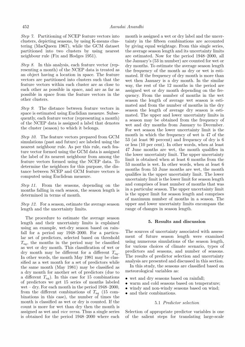
The annual cycle of rainfall for observed histori-cal, NCEP and GCM scenarios (20C3M, A1B, A2and B1) are shown in the first column of figure 4 forthe five time periods considered. This figure givesus general idea about the wet/dry seasons in theregion.

The variation in future season length amongscenarios is high for A2 scenario, whereas it isleast for B1 scenario. This is because amongthe scenarios considered, the scenario A2 has thehighest concentration of carbon dioxide (CO2)equal to 850 ppm, while the same for A1B, B1and COMMIT scenarios are 720 ppm, 550 ppm and≈370 ppm, respectively. Any rise in the concen-tration of CO2 in atmosphere causes the earth’saverage temperature to increase, which in turncauses increase in evaporation especially at lowerlatitudes. The evaporated water would eventuallyprecipitate. In the COMMIT scenario, where theemissions are held the same as in the year 2000,no significant increase in the pattern of projectedfuture season length could be discerned.


Figure 3. Typical results of classification into two seasons (wet and dry) performed using cluster analysis for differentcombinations of the fifteen predictors. (a) Shows the average wet and dry season length. (b and c) Show the upper andlower uncertainty limits in season length due to predictors selected. The period for NCEP and 20C3M is 1948–2000. Thenumbers 1 to 5 in the SRES scenarios represent the five time periods considered in the study namely 2001–2020, 2021–2040,2041–2060, 2061–2080 and 2081–2100, respectively. The grey colour (darker shade) represents the dry season while the lightblue colour (lighter shade) represents the wet season.

5.3 Uncertainties in warm and coolseason length

Based on temperature the study region can bedivided into two seasons namely warm and coldseasons. The sources of uncertainty in warm andcold season length were studied, for choice ofpredictors and climate scenario.

The potential predictors selected for classifica-tion into seasons for different values of Tng forproduct moment correlation between probable pre-dictors in NCEP and GCM datasets are shownin table 5. The classification into seasons was

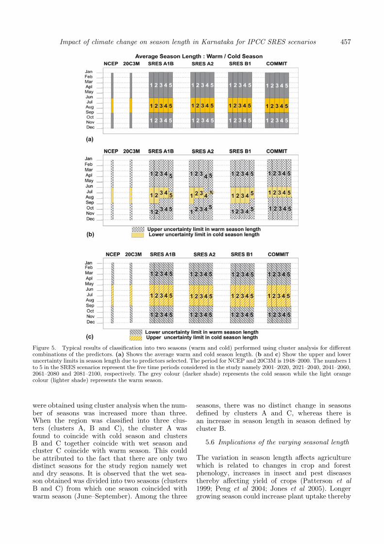
performed for each of the threshold values shown inthe table. The uncertainty in the months selectedas a warm or cold month is subjective to predictorselected for clustering (figure 5).

The average season length and the uncertaintylimits in the season length are estimated quanti-tatively using the various simulations of seasonsobtained for the different combinations of pre-dictor variables (figure 5). The typical results ofuncertainty in the season length for the variouscombinations of predictors selected are shown infigure 5(b and c). It can be observed from thefigure that on an average the warm and cold

456 Aavudai Anandhi

Figure 4. Monthly mean rainfall and average temperatures calculated from NCEP and GCM datasets. The 20C3M andNCEP data are averaged for the period 1948–2000. While for the future SRES scenarios, the five time periods are forthe period 2001–2020, 2021–2040, 2041–2060, 2061–2080 and 2081–2100, respectively. Monthly mean observed rainfall iscalculated for the period 1951–2000.

seasons coincided with wet (June–September) anddry months (rest of them) and there is no changein future warm and cold season length for the fourscenarios (A1B, A2, B1 and COMMIT) considered.However, there is a decrease in warm seasonlength in the lower uncertainty limit in all thefour scenarios considered. The decrease in seasonlength was higher for A2 scenarios when com-pared with the rest of the three scenarios. Thisdecrease in warm season length may be relatedto increase in wet season length, during the sameperiod as observed in the previous section. Theannual cycle of average temperature for NCEP andGCM scenarios (20C3M, A1B, A2 and B1) areshown in the second column of figure 4 for thefive time periods considered. This figure gives usgeneral idea about the warm/cold seasons in theregion.

5.4 Uncertainties in wind and non-windyseason length

Based on wind, the study region can be dividedinto two seasons namely windy and non-windy sea-sons. The classification into seasons was performedfor the each of the threshold values to observethe variability in the length of windy and non-windy seasons. The results of the cluster analysis

Table 5. Potential predictors selected for classificationinto seasons based on temperature for different values ofTng for product moment correlation between probable pre-dictors in NCEP and CGCM3 datasets.

Sl. no. Tng Potential predictors selected

1 1.0–0.95 –2 0.93 Ua 9253 0.76–0.92 Ua 925, Ta 9254 0.56–0.75 Ua 925, Ta 925, Va 925

(not presented for brevity) envisaged that windyand non-windy seasons coincided with wet (June–September) and dry months (rest of them).

Thus the seasons, classified on the basis rainfall,temperature and wind using the predictors fromlarge-scale atmospheric variables, showed that theregion had predominant wet and dry seasons.Hence for studying the variation in season lengthfor varying number of seasons, seasons based onrainfall was used.

5.5 Variation in season length withthe number of seasons

The variation in season length with increase inthe number of seasons was studied. For this pur-pose, the number of seasons was increased fromtwo to five. It was observed that no distinct seasons


Figure 5. Typical results of classification into two seasons (warm and cold) performed using cluster analysis for differentcombinations of the predictors. (a) Shows the average warm and cold season length. (b and c) Show the upper and loweruncertainty limits in season length due to predictors selected. The period for NCEP and 20C3M is 1948–2000. The numbers 1to 5 in the SRES scenarios represent the five time periods considered in the study namely 2001–2020, 2021–2040, 2041–2060,2061–2080 and 2081–2100, respectively. The grey colour (darker shade) represents the cold season while the light orangecolour (lighter shade) represents the warm season.

were obtained using cluster analysis when the num-ber of seasons was increased more than three.When the region was classified into three clus-ters (clusters A, B and C), the cluster A wasfound to coincide with cold season and clustersB and C together coincide with wet season andcluster C coincide with warm season. This couldbe attributed to the fact that there are only twodistinct seasons for the study region namely wetand dry seasons. It is observed that the wet sea-son obtained was divided into two seasons (clustersB and C) from which one season coincided withwarm season (June–September). Among the three

seasons, there was no distinct change in seasonsdefined by clusters A and C, whereas there isan increase in season length in season defined bycluster B.

5.6 Implications of the varying seasonal length

The variation in season length affects agriculturewhich is related to changes in crop and forestphenology, increases in insect and pest diseasesthereby affecting yield of crops (Patterson et al1999; Peng et al 2004; Jones et al 2005). Longergrowing season could increase plant uptake thereby

458 Aavudai Anandhi

increasing evapotranspiration, reducing soilmoisture, reducing the availability of water and airpollution. Longer growing seasons, and especiallyearlier springs, also lead to changes in the hydro-logical cycle with serious negative implicationswhich could lead to water shortage in summer,when the demand is greater (Christidis et al 2007).

The consequences of change in warm and coldseason length are of great importance to agricul-ture since this is closely related to the growthperiod of crops, crop water requirements, the lifecycles of pests (insects and parasites) infecting thecrops. The evaporation from water bodies are influ-enced by the change in warm seasons especially inarid and semi-arid regions. Temperature influencesplant growth and increase evaporation/evapotrans-piration of crops.

The most likely impact of climate change in plantdiseases will be felt in three areas:

(1) losses from plant diseases,(2) efficacy of disease management strategies, and(3) the geographical distribution of plant diseases.

Climate change could have positive, negative orno impact on individual plant diseases (Chakra-borty et al 2000).

The ill effects of increase in windy season includeincrease in the rate of evaporation of water,increase in aridity, poor crop growth and reduc-tion in yield due to mechanical damage to crops(e.g., stripping of leaves, abrasion in plant canopiesthrough rubbing, Cleugh et al 1998).

6. Summary and conclusions

Changes in seasons and season length of a regionare driven by shifts in the intensity of sunlightreaching earth’s surface (insolation), latitude, con-tinental and marine climate, wind direction, andlocal geographical features. Since change in seasonlength is an indicator, as well as an effect, of climatechange and is less studied, the objective of thisstudy was set to investigate the variability of futureseason length to some of the uncertainties such asthe choice of climate scenario, predictors, definitionof seasons and number of seasons.

For this purpose four climate scenarios rele-vant to IPCC’s AR4 report namely A1B, A2,B1 and COMMIT were used. The seasons weredefined based on the three meteorological vari-ables (namely, rainfall, temperature and wind)using large scale atmospheric variables (predictors)which have physical relationship to these vari-ables. Wet and dry seasons were defined basedon rainfall, warm and cold seasons were definedbased on temperature, windy and non-windy

seasons based on wind. The predictors from NCEPreanalysis (period: 1948–2000) and Canadian GCM(CGCM3.1, period: 1948–2100) were used in thisstudy. The classifications into seasons were carriedout using K-means clustering technique and near-est neighbour rule. The chosen methodology wastested for the Karnataka state in India.

The results showed:

• Uncertainty in season length for the choice ofpredictors for the different seasonal definitionsused in the study.

• The region has predominant wet and dryseasons.

• Average wet season increased in future towardsthe end of the 21st century for A2, A1B and B1scenarios. The variation is high for A2 scenario,whereas it is least for B1 scenario. No change inCOMMIT scenario. Similar pattern of increaseis observed in upper and lower uncertainty limitsin wet and dry season length.

• No change in average and upper uncertaintylimits for warm and cold seasons in future for allthe four scenarios. However, there is a decreasein warm season length in the lower uncertaintylimit. The decrease in season length was higherfor A2 scenarios when compared with the rest ofthe scenarios.

• The windy and non-windy seasons coincidedwith wet and dry seasons.

• When the number of seasons were increasedfrom two to five, the results of the analy-sis revealed that the distinct cluster could notbe obtained when the number of seasons wereincreased beyond three. When the region wasclassified into three clusters, three distinct sea-sons were obtained and they coincide with cold,warm and wet seasons.

The present study brings out the variability inseason length across scenarios, season type, andwhen the number of seasons is changed. The uncer-tainties in the season length to the choice ofclustering methods and GCMs should also beconsidered to provide more general conclusionsabout the variation in the study region whichwould help policy makers and general public forrealistic assessment, management and mitigationof natural disasters, and for sustainable develop-ment. Investigating these uncertainties is a futurescope of study.

Acknowledgements

The author thanks Prof. D Nagesh Kumar,Dr V V Srinivas, Prof. Ravi Nanjundiah, Dr RRavi, Dr Muthuswamy Murugan, Prof. GauthamSethi and Dr R K Yadav and the anonymous


reviewers for their support, encouragement andvaluable inputs. The support from the IndianInstitute of Science to carry out the research workis acknowledged.

Annexure: Dependence measures

Three dependence measures used in this studyare product moment correlation (Pearson 1896),Spearman’s rank correlation (Spearman 1904a,1904b), and Kendall’s tau (Kendall 1951).

Let the probable predictor and predictand formonth t be denoted as Xt and Yt, respectively.Then the product moment correlation which mea-sures the linear relationship between probablepredictor and predictand is given by:

P =∑N

t=1(Xt − X)(Yt − Y )NσXσY

,

where N refers to the number of months in thedatasets; X and Y represent the means of predic-tor and predictand respectively, while σX and σY

represent the standard deviations of the same.Spearman’s rank correlation and Kendall’s tau

are the two nonparametric correlations used inthis study which are estimated based on ranksassigned to data points in predictor and predictanddatasets. The advantage of these rank correlationsover the linear correlation stems from the use ofranks rather than numerical values of the predictorand the predictand variables for estimation of thecorrelations (Press et al 1992). Ranks are assignedto the N data points in each dataset after arrang-ing them in increasing order of magnitude, suchthat the least value in the data has the first rank.Spearman’s rank correlation (ρ) is computed usingthe difference between the ranks of contempo-raneous values of predictor and predictand (Di).

ρ = 1 − 6∑N

i=1 D2i

N(N 2 − 1),

where Di = Rank of Xt − Rank of Yt.Estimation of the Kendall’s tau (τ) for a

pair of predictor and predictand datasets involvespreparation of N pairs of data ranks {(ui, vi),i = 1, . . . , N}, where ui and vi denote ranks ofcontemporaneous data points in the predictorand predictand datasets at ith time step respec-tively. Let two pairs of ranks be (uj, vj) and(uk, vk). The two pairs are concordant if uj > uk

and vj > vk, or if uj < uk and vj < vk, for which(uj − uk)(vj − vk) > 0. The two pairs are discor-dant, if uj > uk and vj < vk, or if uj < uk and

vj > vk, for which (uj − uk)(vj − vk) < 0. A tiedpair is neither concordant nor discordant, i.e.,(uj − uk)(vj − vk) = 0. The Kendall’s τ is calcu-lated using the formula given below.

τ =4λ

N(N − 1)/2,

where λ is the difference between the number ofconcordant pairs and the number of discordantpairs. So, a high value of λ means that most pairsare concordant, indicating that the two rankingsare consistent. Further, N(N − 1)/2 is the totalnumber of possible pairs of ranks. If there are alarge number of tied pairs it should be adjustedaccordingly. A positive value of τ indicates thatthe ranks of both the variables increase together,whilst a negative correlation indicates that as therank of one variable increases the rank of theother decreases. The Kendall coefficient has twoadvantages over the Spearman coefficient (Leach1979). The first advantage is that it is appro-priate when a large number of ties are presentwithin ranks. The second advantage is its directand simple interpretation in terms of probabili-ties of observing concordant and discordant pairs.The Spearman’s coefficient can be considered asthe regular Pearson’s correlation coefficient interms of the proportion of variability accountedfor, whereas Kendall’s coefficient represents aprobability, i.e., the difference between the prob-abilities that the observed data are in the sameorder and the observed data are not in the sameorder. The advantages of Kendall coefficient makesit useful to effectively interpret the relationshipbetween the predictors in NCEP and GCM datasets and between predictors in NCEP and thepredictand.

References

Alley R, Berntsen T, Bindoff N L, Chen Z, Chidthaisong A,Friedlingstein P, Gregory J, Hegerl G, Heimann M,Hewitson B, Hoskins B, Joos F, Jouzel J, Kattsov V,Lohmann U, Manning M, Matsuno T, Molina M,Nicholls N, Overpeck J, Qin D, Raga G, Ramaswamy V,Ren J, Rusticucci M, Solomon S, Somerville R,Stocker T F, Stott P, Stouffer R J, Whetton P,Wood R A and Wratt D 2007 Climate Change 2007:The Physical Science Basis. Summary for Policy makers;Report of the Intergovernmental Panel on ClimateChange, Geneva, CH.

Anandhi A 2007 Impact assessment of climate change onhydrometeorology of Indian river basin for IPCC SRESscenarios; PhD thesis, Indian Institute of Science, India.

Anandhi A, Srinivas V V, Nanjundiah R S and Kumar D N2008 Downscaling precipitation to river basin in India forIPCC SRES scenarios using support vector machine; Int.J. Climatol. 28(3) 401–420.

460 Aavudai Anandhi

Argiriou A A, Kassomenos P A and Lykoudis S P 2004 Onthe methods for the delimitation of seasons: Water, Air,and Soil Pollution; Focus 4 65–74.

Chakraborty S, Tiedemann A V and Teng P S 2000 Climatechange: Potential impact on plant diseases; Environmen-tal Pollution 108 317–326.

Christidis N, Stott P A, Brown S, Karoly D J and Caesar J2007 Human contribution to the lengthening of the grow-ing season during 1950–99; J. Climate 20 5441–5454.

Cleugh H A, Miller J M and Bohm M 1998 Directmechanical effects of wind on crops; Agroforestry Systems41(1) 85–112, 10.1023/A:1006067721039.

Doty B and Kinter J L III 1993 The grid analysis and displaysystem (GrADS): A desktop tool for earth science visuali-zation; American Geophysical Union 1993 Fall Meeting,San Fransico, CA, 6–10 December.

Fix E and Hodges J L 1951 Discriminatory analysis: Non-parametric discrimination: Consistency properties; USAFSchool of Aviation Medicine, Project 21-49-004, Report 4.

Jones G S, Jones A, Roberts D L, Stott P A andWilliams K D 2005 Sensitivity of global scale climatechange attribution results to inclusion of fossil fuel blackcarbon aerosol; Geophys. Res. Lett. 32 L14701, doi:10.1029/2005GL023370.

Kalnay E, Kanamitsu M, Kistler R, Collins W,Deaven D, Gandin L, Iredell M, Saha S, White G,Woollen J, Zhu Y, Chelliah M, Ebisuzaki W, Higgins W,Janowiak J, Mo K C, Ropelewski C, Wang J, Leetmaa A,Reynolds R, Jenne R and Joseph D 1996 TheNCEP/NCAR 40-year reanalysis project; Bull. Amer.Meteor. Soc. 77(3) 437–471.

Kendall M G 1951 Regression structure and functional rela-tionship, Part I; Biometrika 38 11–25.

Kripalani R H, Oh J H, Kulkarni A, Sabade S S andChaudhari H S 2007 South Asian summer monsoon pre-cipitation variability: Coupled climate model simula-tions and projections under IPCC AR4; Theoretical andApplied Climatology 90 133–159.

Lamb H H 1972 British Isles weather types and a register ofdaily sequence of circulation patterns, 1861–1971; Geo-physical Memoir 116 HMSO, London, pp. 85.

Leach C 1979 Introduction to statistics: A nonparametricapproach for the social sciences (New York: Wiley).

MacQueen J 1967 Some methods for classification andanalysis of multivariate observation; In: Proceedings of thefifth Berkeley Symposium on mathematical statistics andprobability, (eds) Le Cam L M and Neyman J (Berkeley:University of California Press) 1 281–297.

Nakicenovic N, Alcamo J, Davis G, de Vries B,Fenhann J, Gaffin S, Gregory K, Grubler A, Jung T Y,Kram T, La Rovere E L, Michaelis L, Mori S, Morita T,Pepper W, Pitcher H, Price L, Raihi K, Roehrl A,Rogner H H, Sankovski A, Schlesinger M, Shukla P,Smith S, Swart R, van Rooijen S, Victor N andDadi Z 2000 IPCC Special report on emissions scenarios,Cambridge University Press, Cambridge, United King-dom and New York, NY, USA, pp. 599.

Patterson D T, Westbrook J K, Joyce R J V, Lingren P Dand Rogasik J 1999 Weeds, insects and diseases; ClimaticChange 43 711–727.

Pearson K 1896 Mathematical contributions to the Theoryof Evolution III Regression Heredity and Panmixia;

Philosophical Transactions of the Royal Society ofLondon Series 187 253–318.

Peng S, Huang J, Sheeshy J E, Laza R C, Visperas R M,Zhong X, Centeno G S, Khush G S and Cassman K G2004 Rice yields decline with higher night temperaturefrom global warming; Proceedings of National Academyof Science, USA 101 9971–9975.

Press W H, Teukolsky S A, Vetterling W T andFlannery B P 1992 Numerical recipes in Fortran 77:The art of scientific computing (New York: CambridgeUniversity Press).

Rajeevan M, Bhate J, Kale J D and Lal B 2005 Developmentof a high resolution daily gridded rainfall data for theIndian Region (version 2), Meteorol. Monogr. Climatol.22/2005, India Meteorol. Dept., New Delhi.

Rajeevan M, Bhate J, Kale J D and Lal B 2006 Highresolution daily gridded rainfall data for the Indianregion: Analysis of break and active monsoon spells;Curr. Sci. 91(3) 296–306.

Rupa Kumar K, Sahai A K, Krishna Kumar K,Patwardhan S K, Mishra P K, Revadekar J V, Kamala Kand Pant G B 2006 High-resolution climate changescenarios for India for the 21st century; Curr. Sci. 90334–344.

Sailor D J, Smith M and Hart M 2008 Climate change impli-cations for wind power resources in the Northwest UnitedStates; Renewable Energy 33 2393–2406.

Spearman C E 1904a ‘General intelligence’ objectivelydetermined and measured; Am. J. Psychol. 5 201–293.

Spearman C E 1904b Proof and measurement of associationbetween two things; Am. J. Psychol. 15 72–101.

Tripathi S, Srinivas V V and Nanjundiah R S 2006 Down-scaling of precipitation for climate change scenarios:A support vector machine approach; J. Hydrol. 330621–640, doi: 10.1016/j.jhydrol.2006.04.030.

Tuller S E 1990 Standard seasons; Int. J. Biomet. 34181–188.

Winkler J A, Palutikof J P, Andresen J A and Goodess C M1997 The simulation of daily temperature time series fromGCM output Part II: Sensitivity analysis of an empiri-cal transfer function methodology; J. Climate 10(10)2514–2532.

Yadav R K, Rupa Kumar K and Rajeevan M 2007 Roleof Indian Ocean sea surface temperatures in modu-lating northwest Indian winter precipitation variabi-lity; Theoretical and Applied Climatology 87 73–83, doi:10.1007/s00704005-0221.

Yadav R K, Rupa Kumar K and Rajeevan M 2009aIncreasing influence of ENSO and decreasing influence ofAO/NAO in the recent decades over northwest India win-ter precipitation; J. Geophys. Res.-Atmos. 114 D12112,doi: 10.1029/2008JD011318.

Yadav R K, Rupa Kumar K and Rajeevan M 2009b Out-of-phase relationships between convection over north-westIndia and warm-pool region during winter season; Int.J. Climatol. 29 1330–1338, doi: 10.1002/joc.1783.

Yadav R K, Rupa Kumar K and Rajeevan M 2010a Climatechange scenarios for northwest India winter season; Qua-ternary International 213 12–19.

Yadav R K, Yoo J H, Kucharski F and Abid M A 2010bWhy is ENSO influencing northwest India winter precipi-tation in recent decades?; J. Climate (in press).

MS received 21 August 2009; revised 8 May 2010; accepted 31 May 2010

Documents

Assessing impact of climate change on season length in