Assessing expression data quality in high-density oligonucliotide arrays

Outline

• GeneChip® technology

• Affymetrix QC recommendations

• Review of models for expression value estimation

• Assessing chip expression data quality

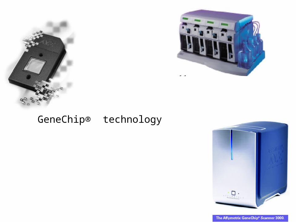
GeneChip® technology

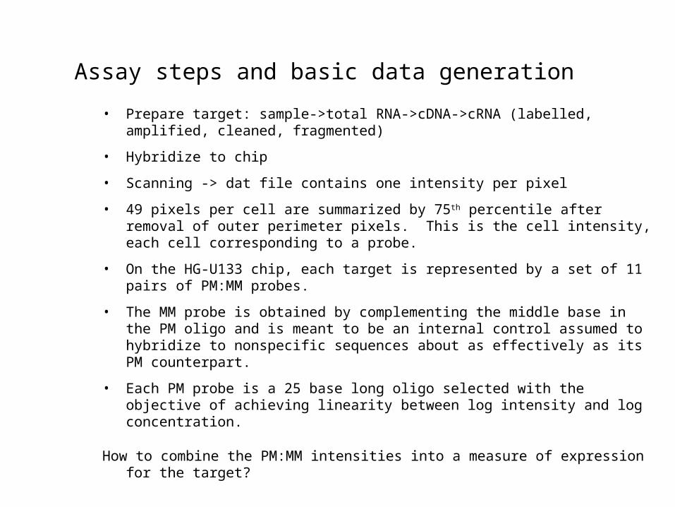
Assay steps and basic data generation

• Prepare target: sample->total RNA->cDNA->cRNA (labelled, amplified, cleaned, fragmented)

• Hybridize to chip

• Scanning -> dat file contains one intensity per pixel

• 49 pixels per cell are summarized by 75th percentile after removal of outer perimeter pixels. This is the cell intensity, each cell corresponding to a probe.

• On the HG-U133 chip, each target is represented by a set of 11 pairs of PM:MM probes.

• The MM probe is obtained by complementing the middle base in the PM oligo and is meant to be an internal control assumed to hybridize to nonspecific sequences about as effectively as its PM counterpart.

• Each PM probe is a 25 base long oligo selected with the objective of achieving linearity between log intensity and log concentration.

How to combine the PM:MM intensities into a measure of expression for the target?

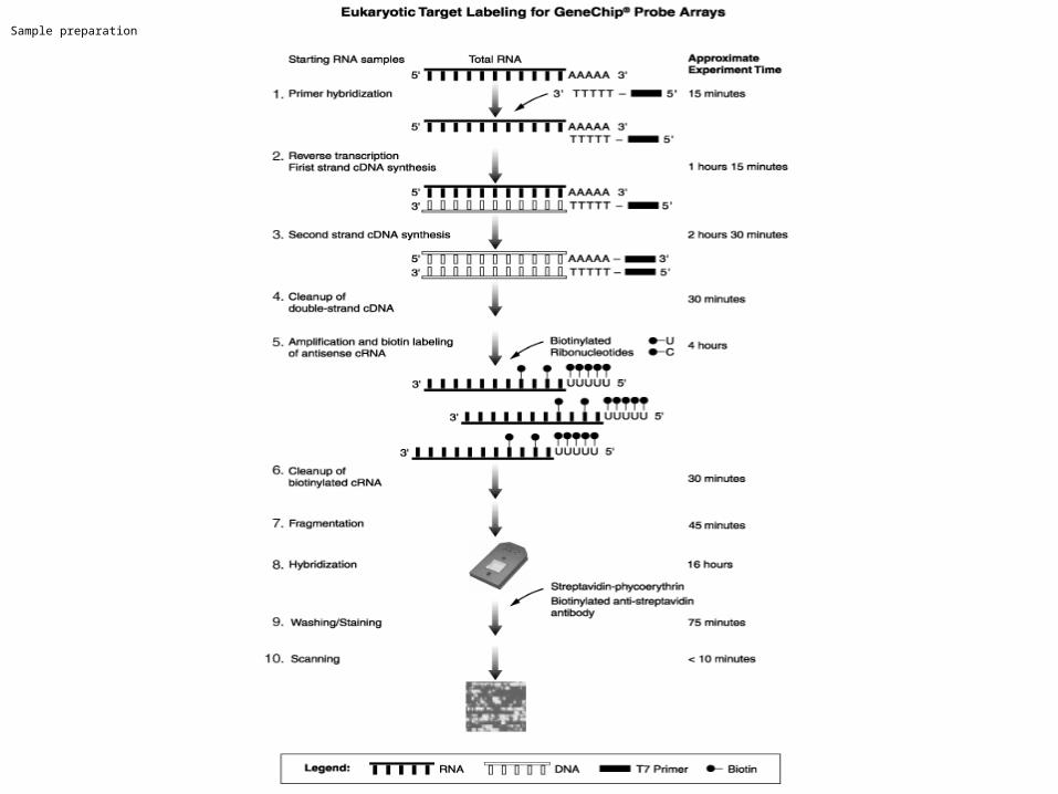
Sample preparation

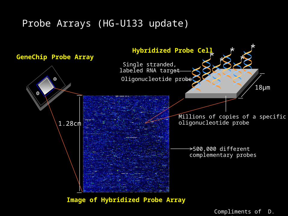
Probe Arrays (HG-U133 update)

18µm18µm

Millions of copies of a specificMillions of copies of a specificoligonucleotide probeoligonucleotide probe

Image of Hybridized Probe ArrayImage of Hybridized Probe Array

>500,000 different>500,000 differentcomplementary probes complementary probes

Single stranded, Single stranded, labeled RNA targetlabeled RNA target

Oligonucleotide probeOligonucleotide probe

**

**

*

1.28cm1.28cm

GeneChipGeneChip Probe ArrayProbe ArrayHybridized Probe CellHybridized Probe Cell

Compliments of D. Gerhold

Affymetrix QC recommendations

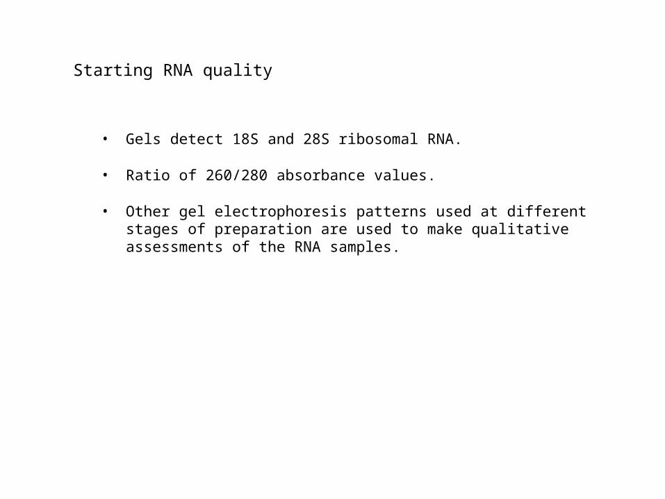
Starting RNA quality

• Gels detect 18S and 28S ribosomal RNA.

• Ratio of 260/280 absorbance values.

• Other gel electrophoresis patterns used at different stages of preparation are used to make qualitative assessments of the RNA samples.

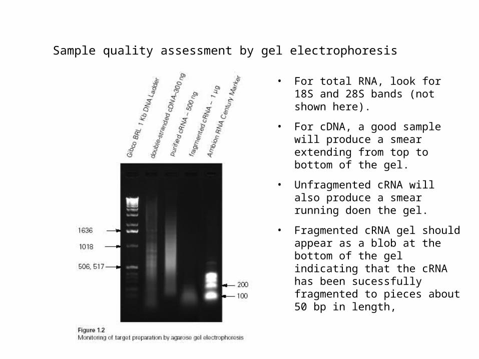
Sample quality assessment by gel electrophoresis

• For total RNA, look for 18S and 28S bands (not shown here).

• For cDNA, a good sample will produce a smear extending from top to bottom of the gel.

• Unfragmented cRNA will also produce a smear running doen the gel.

• Fragmented cRNA gel should appear as a blob at the bottom of the gel indicating that the cRNA has been sucessfully fragmented to pieces about 50 bp in length,

Next slide from Vanderbilt MicroArray Shared Resource web site

• http://array.mc.vanderbilt.edu/Pages/VMSR_Info/Sample_submission.htm

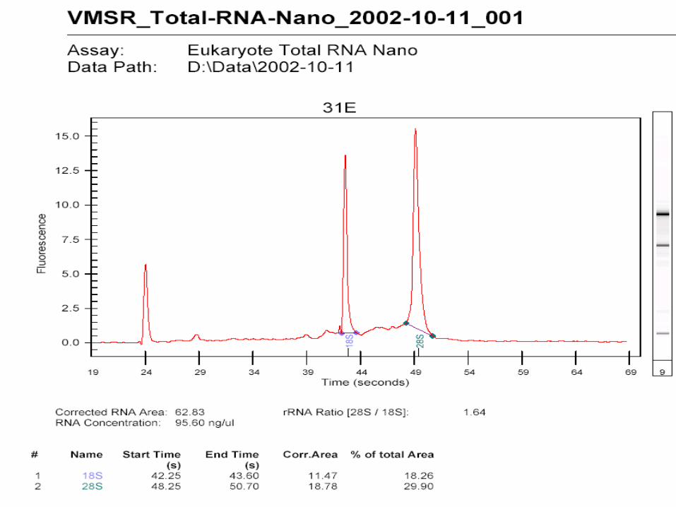
http://array.mc.vanderbilt.edu/Pages/VMSR_Info/Sample_submission.htm

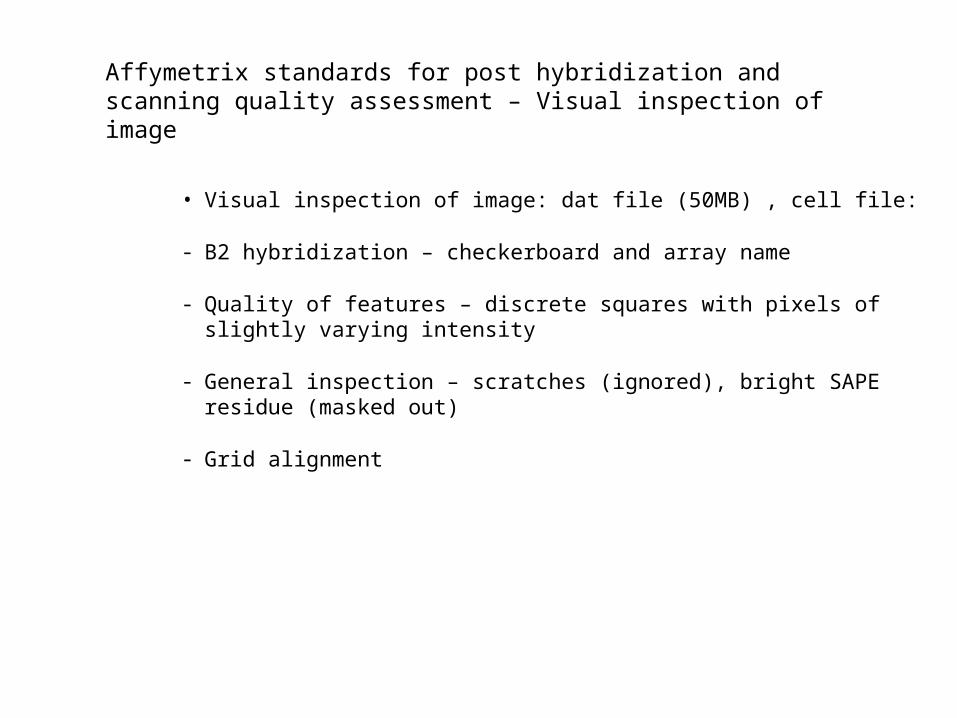
Affymetrix standards for post hybridization and scanning quality assessment – Visual inspection of image

• Visual inspection of image: dat file (50MB) , cell file:

- B2 hybridization – checkerboard and array name

- Quality of features – discrete squares with pixels of slightly varying intensity

- General inspection – scratches (ignored), bright SAPE residue (masked out)

- Grid alignment

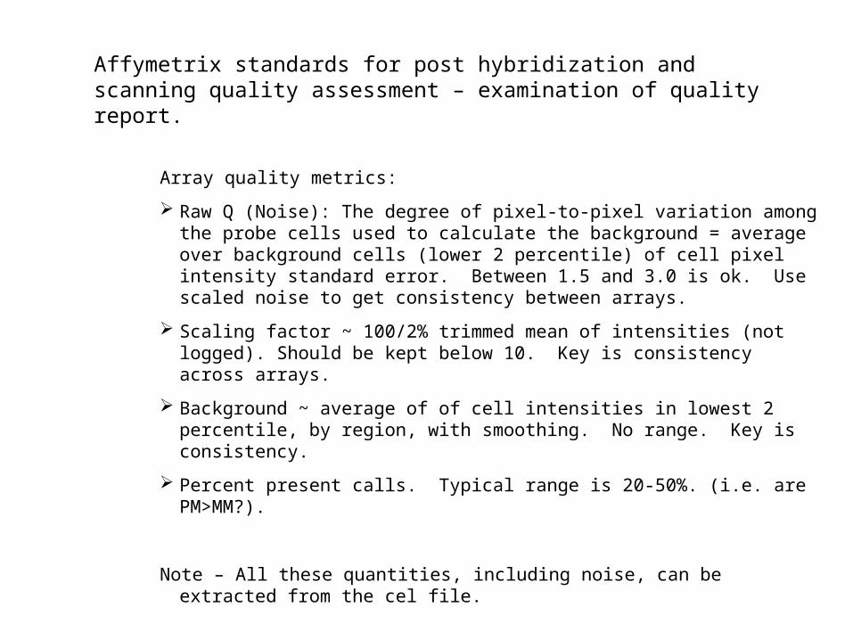
Affymetrix standards for post hybridization and scanning quality assessment – examination of quality report.

Array quality metrics:

Raw Q (Noise): The degree of pixel-to-pixel variation among the probe cells used to calculate the background = average over background cells (lower 2 percentile) of cell pixel intensity standard error. Between 1.5 and 3.0 is ok. Use scaled noise to get consistency between arrays.

Scaling factor ~ 100/2% trimmed mean of intensities (not logged). Should be kept below 10. Key is consistency across arrays.

Background ~ average of of cell intensities in lowest 2 percentile, by region, with smoothing. No range. Key is consistency.

Percent present calls. Typical range is 20-50%. (i.e. are PM>MM?).

Note – All these quantities, including noise, can be extracted from the cel file.

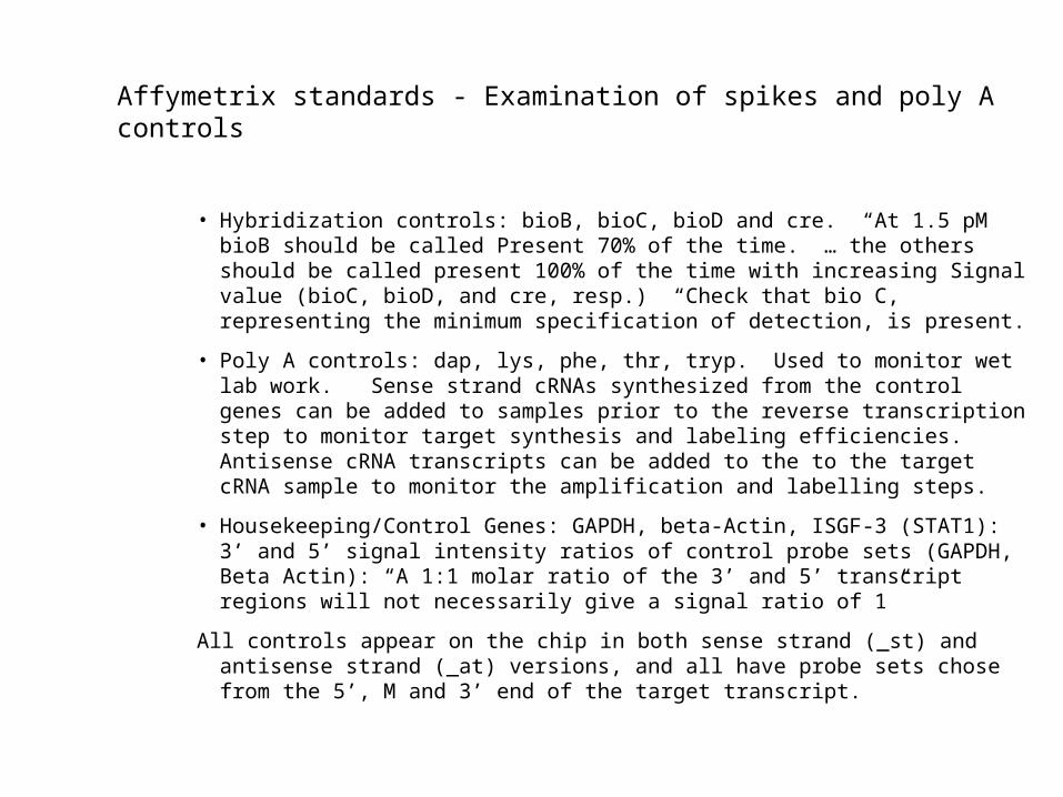
Affymetrix standards - Examination of spikes and poly A controls

• Hybridization controls: bioB, bioC, bioD and cre. “At 1.5 pM bioB should be called Present 70% of the time. … the others should be called present 100% of the time with increasing Signal value (bioC, bioD, and cre, resp.) “Check that bio C, representing the minimum specification of detection, is present.

• Poly A controls: dap, lys, phe, thr, tryp. Used to monitor wet lab work. Sense strand cRNAs synthesized from the control genes can be added to samples prior to the reverse transcription step to monitor target synthesis and labeling efficiencies. Antisense cRNA transcripts can be added to the to the target cRNA sample to monitor the amplification and labelling steps.

• Housekeeping/Control Genes: GAPDH, beta-Actin, ISGF-3 (STAT1): 3’ and 5’ signal intensity ratios of control probe sets (GAPDH, Beta Actin): “A 1:1 molar ratio of the 3’ and 5’ transcript regions will not necessarily give a signal ratio of 1”

All controls appear on the chip in both sense strand (_st) and antisense strand (_at) versions, and all have probe sets chose from the 5’, M and 3’ end of the target transcript.

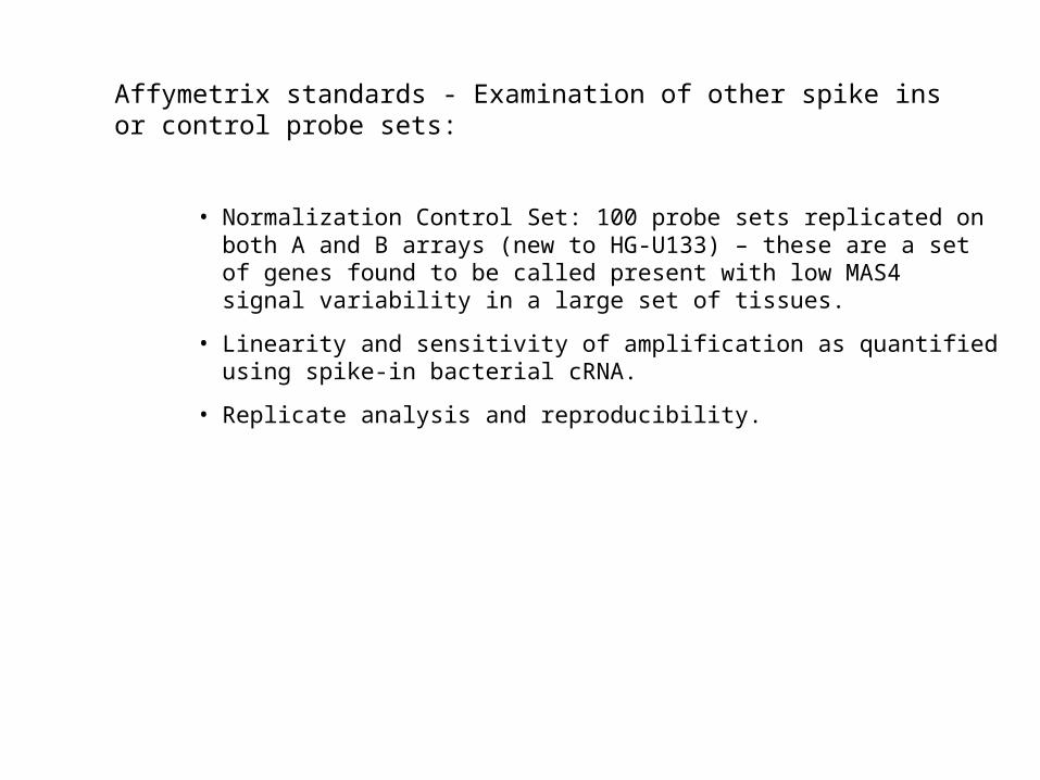
Affymetrix standards - Examination of other spike ins or control probe sets:

• Normalization Control Set: 100 probe sets replicated on both A and B arrays (new to HG-U133) – these are a set of genes found to be called present with low MAS4 signal variability in a large set of tissues.

• Linearity and sensitivity of amplification as quantified using spike-in bacterial cRNA.

• Replicate analysis and reproducibility.

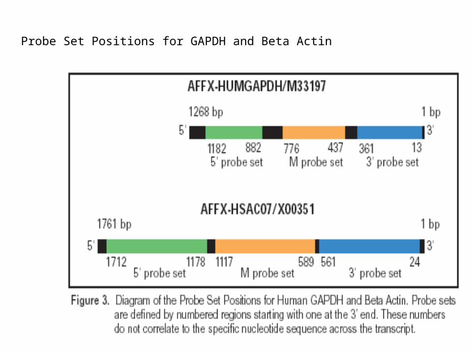
Probe Set Positions for GAPDH and Beta Actin

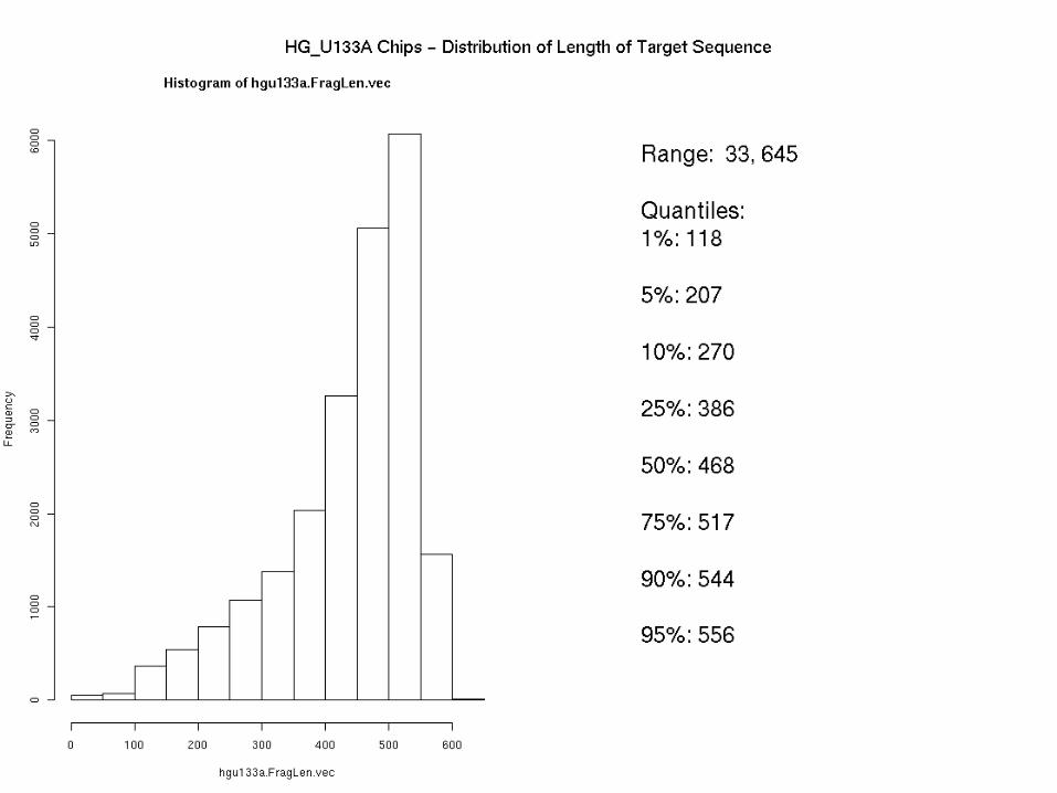
Length of target sequences on HG-U133A chip

Examination of dat file

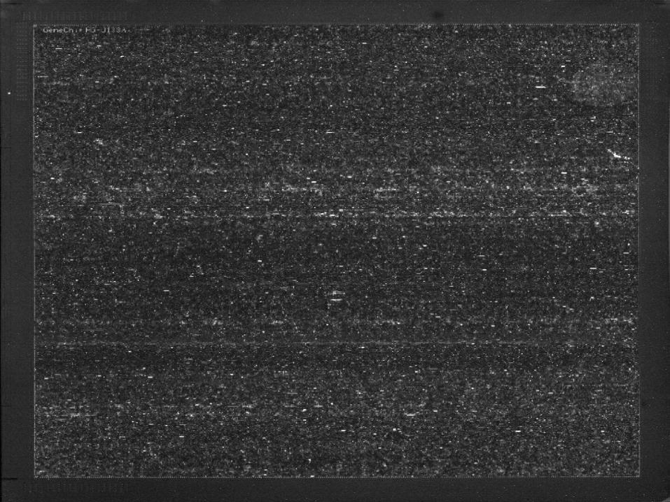
Chip dat file - full

Chip dat file – checkered board – oligo B2

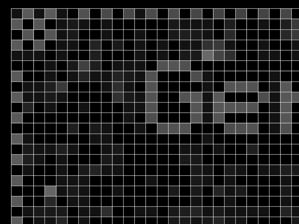
Chip dat file – checkered board – close up

Chip dat file – checkered board – close up w/ grid

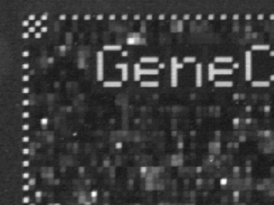
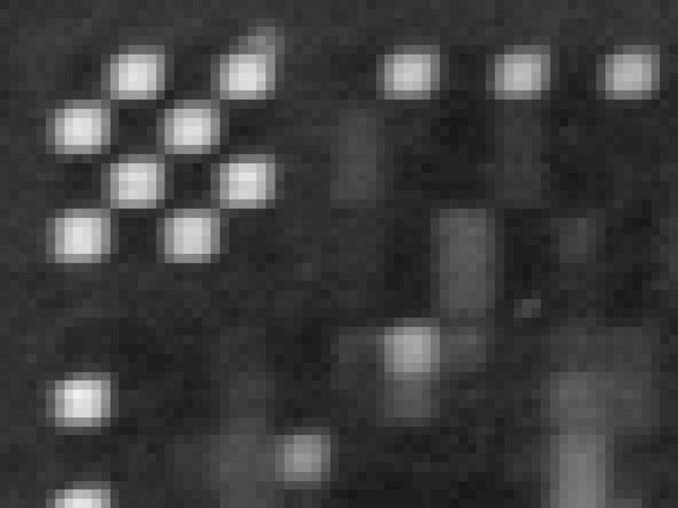
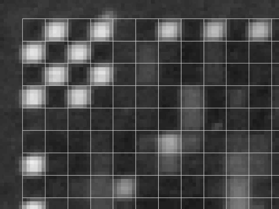
Examination of cel file

Chip cel file – checkered board

Chip cel file – checkered board – close up w/ grid

Chip cel file – PM - MM

Limitatons of standard QC metrics and procedure

• Link between these metrics and the numbers we care about is missing.

• Quality of data gauged from spike-ins requiring special processing may not represent the quality of the rest of the data on the chip – risk of QCing the chip QC process itself, but not the gene expression data.

Good end-point data quality assessment is needed to assess the validity of these indirect data quality assessments.

Review of models for gene expression value estimation

MAS 5 (Microarray Suite 5 by Affymetrix)

Expression measures are derived as follows in Affymetrix’ Microarray Analysis Suite 5.0:

• A background correction is applied to the probe intensities.

• For each probe set the log expression is estimated by means of a one-step Tukey biweighted average of log(PMj- MMj

*), where MM* is an MM value modified to ensure that it does not exceed the PM value. This is equivalent to robustly estimating the parameter in the model log(PMj- MMj

*) = + ej

• To compare expression measures across chips, expression values are normalized by a multiplicative scaling factor. This is equivalent to shifting the expression values on the log scale.

See Affy technical description [1].

RMA

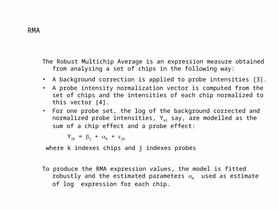
The Robust Multichip Average is an expression measure obtained from analysing a set of chips in the following way:

• A background correction is applied to probe intensities [3].• A probe intensity normalization vector is computed from the set of chips and

the intensities of each chip normalized to this vector [4].• For one probe set, the log of the background corrected and normalized probe

intensities, Yki say, are modelled as the sum of a chip effect and a probe effect:

Yjk = j + k + jk

where k indexes chips and j indexes probes

To produce the RMA expression values, the model is fitted robustly and the estimated parameters k used as estimate of log expression for each chip.

RMA vs MAS5

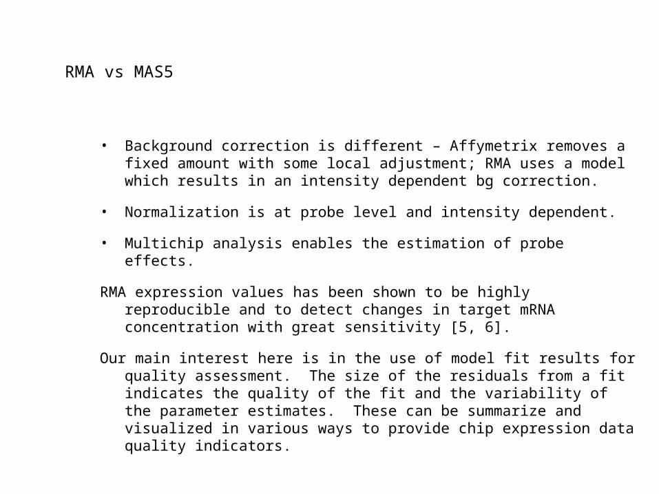
• Background correction is different – Affymetrix removes a fixed amount with some local adjustment; RMA uses a model which results in an intensity dependent bg correction.

• Normalization is at probe level and intensity dependent.

• Multichip analysis enables the estimation of probe effects.

RMA expression values has been shown to be highly reproducible and to detect changes in target mRNA concentration with great sensitivity [5, 6].

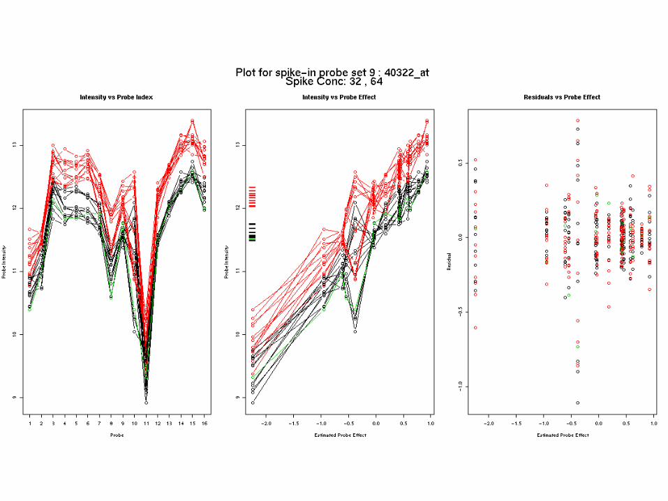
Our main interest here is in the use of model fit results for quality assessment. The size of the residuals from a fit indicates the quality of the fit and the variability of the parameter estimates. These can be summarize and visualized in various ways to provide chip expression data quality indicators.

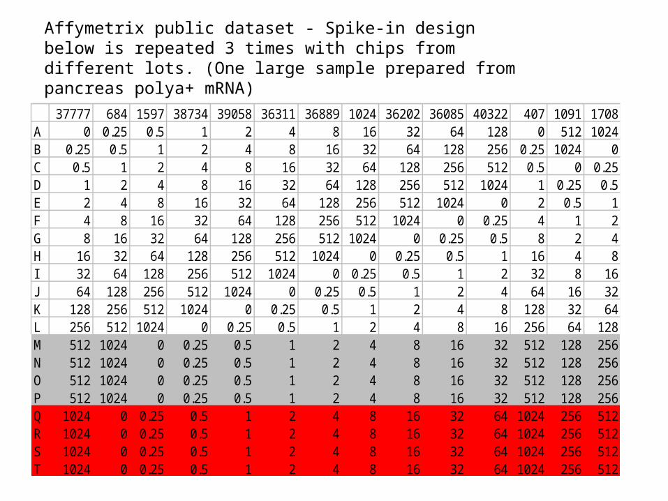
Affymetrix public dataset - Spike-in design below is repeated 3 times with chips from different lots. (One large sample prepared from pancreas polya+ mRNA)

37777 684 1597 38734 39058 36311 36889 1024 36202 36085 40322 407 1091 1708A 0 0.25 0.5 1 2 4 8 16 32 64 128 0 512 1024B 0.25 0.5 1 2 4 8 16 32 64 128 256 0.25 1024 0C 0.5 1 2 4 8 16 32 64 128 256 512 0.5 0 0.25D 1 2 4 8 16 32 64 128 256 512 1024 1 0.25 0.5E 2 4 8 16 32 64 128 256 512 1024 0 2 0.5 1F 4 8 16 32 64 128 256 512 1024 0 0.25 4 1 2G 8 16 32 64 128 256 512 1024 0 0.25 0.5 8 2 4H 16 32 64 128 256 512 1024 0 0.25 0.5 1 16 4 8I 32 64 128 256 512 1024 0 0.25 0.5 1 2 32 8 16J 64 128 256 512 1024 0 0.25 0.5 1 2 4 64 16 32K 128 256 512 1024 0 0.25 0.5 1 2 4 8 128 32 64L 256 512 1024 0 0.25 0.5 1 2 4 8 16 256 64 128M 512 1024 0 0.25 0.5 1 2 4 8 16 32 512 128 256N 512 1024 0 0.25 0.5 1 2 4 8 16 32 512 128 256O 512 1024 0 0.25 0.5 1 2 4 8 16 32 512 128 256P 512 1024 0 0.25 0.5 1 2 4 8 16 32 512 128 256Q 1024 0 0.25 0.5 1 2 4 8 16 32 64 1024 256 512R 1024 0 0.25 0.5 1 2 4 8 16 32 64 1024 256 512S 1024 0 0.25 0.5 1 2 4 8 16 32 64 1024 256 512T 1024 0 0.25 0.5 1 2 4 8 16 32 64 1024 256 512

The model fits – ex 1

The model fits – ex 2

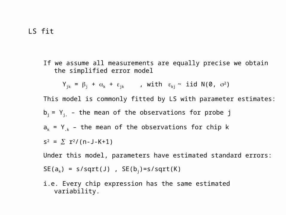
LS fit

If we assume all measurements are equally precise we obtain the simplified error model

Yjk = j + k + jk , with kj ~ iid N(0, 2)

This model is commonly fitted by LS with parameter estimates:

bj = Yj. – the mean of the observations for probe j

ak = Y.k – the mean of the observations for chip k

s2 = r2/(n-J-K+1)

Under this model, parameters have estimated standard errors:

SE(ak) = s/sqrt(J) , SE(bj)=s/sqrt(K)

i.e. Every chip expression has the same estimated variability.

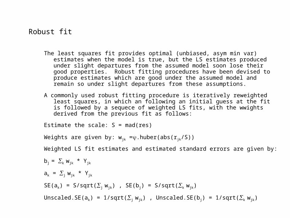
Robust fit

The least squares fit provides optimal (unbiased, asym min var) estimates when the model is true, but the LS estimates produced under slight departures from the assumed model soon lose their good properties. Robust fitting procedures have been devised to produce estimates which are good under the assumed model and remain so under slight departures from these assumptions.

A commonly used robust fitting procedure is iteratively reweighted least squares, in which an following an initial guess at the fit is followed by a sequece of weighted LS fits, with the wwights derived from the previous fit as follows:

Estimate the scale: S = mad(res)

Weights are given by: wjk =.huber(abs(rjk/S))

Weighted LS fit estimates and estimated standard errors are given by:

bj = k wjk * Yjk

ak = j wjk * Yjk

SE(ak) = S/sqrt(j wjk) , SE(bj) = S/sqrt(k wjk)

Unscaled.SE(ak) = 1/sqrt(j wjk) , Unscaled.SE(bj) = 1/sqrt(k wjk)

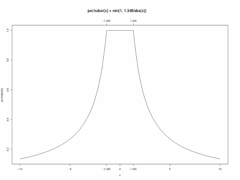
Huber function

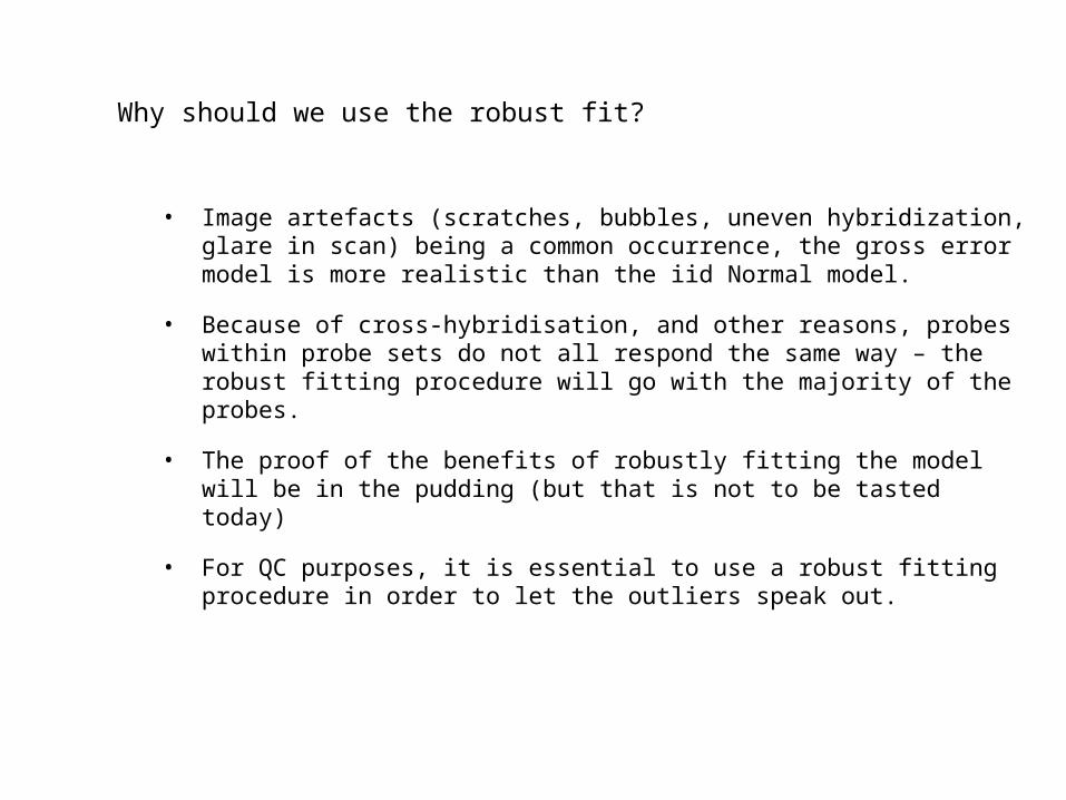
Why should we use the robust fit?

• Image artefacts (scratches, bubbles, uneven hybridization, glare in scan) being a common occurrence, the gross error model is more realistic than the iid Normal model.

• Because of cross-hybridisation, and other reasons, probes within probe sets do not all respond the same way – the robust fitting procedure will go with the majority of the probes.

• The proof of the benefits of robustly fitting the model will be in the pudding (but that is not to be tasted today)

• For QC purposes, it is essential to use a robust fitting procedure in order to let the outliers speak out.

Assessing chip expression data quality

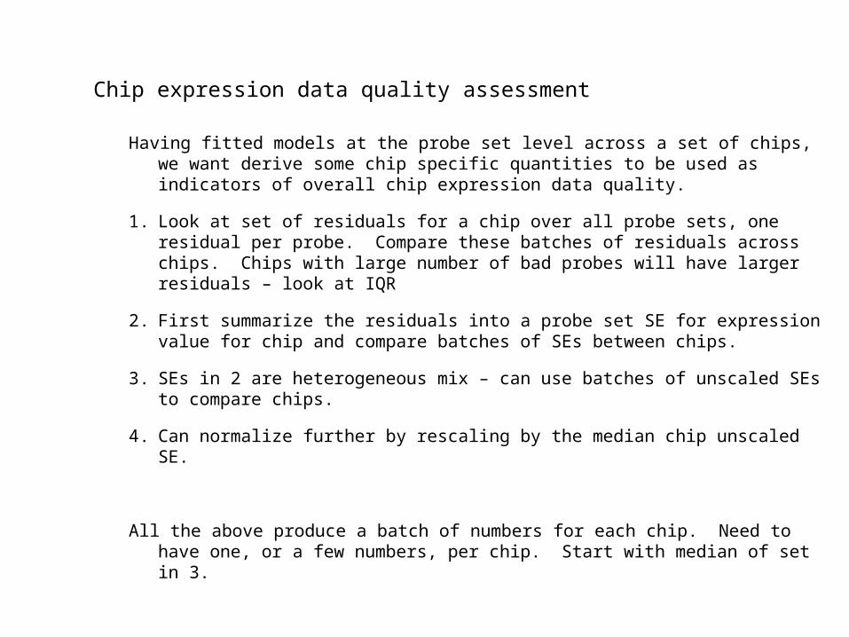
Chip expression data quality assessment

Having fitted models at the probe set level across a set of chips, we want derive some chip specific quantities to be used as indicators of overall chip expression data quality.

1. Look at set of residuals for a chip over all probe sets, one residual per probe. Compare these batches of residuals across chips. Chips with large number of bad probes will have larger residuals – look at IQR

2. First summarize the residuals into a probe set SE for expression value for chip and compare batches of SEs between chips.

3. SEs in 2 are heterogeneous mix – can use batches of unscaled SEs to compare chips.

4. Can normalize further by rescaling by the median chip unscaled SE.

All the above produce a batch of numbers for each chip. Need to have one, or a few numbers, per chip. Start with median of set in 3.

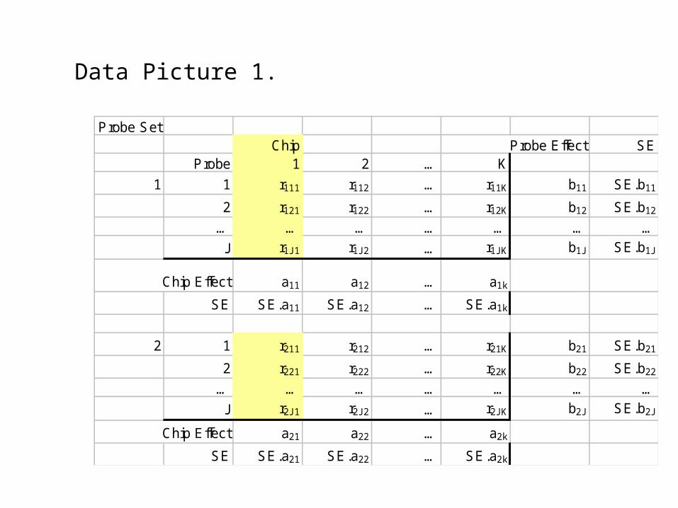
Data Picture 1.

Probe SetChip Probe Effect SE

Probe 1 2 … K

1 1 r111 r112 … r11K b11 SE.b11

2 r121 r122 … r12K b12 SE.b12

… … … … … … …

J r1J1 r1J2 … r1JK b1J SE.b1J

Chip Effect a11 a12 … a1k

SE SE.a11 SE.a12 … SE.a1k

2 1 r211 r212 … r21K b21 SE.b21

2 r221 r222 … r22K b22 SE.b22

… … … … … … …

J r2J1 r2J2 … r2JK b2J SE.b2J

Chip Effect a21 a22 … a2k

SE SE.a21 SE.a22 … SE.a2k

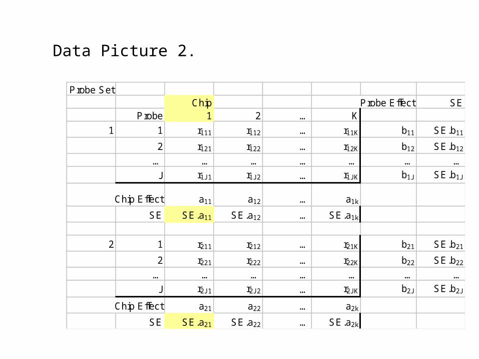
Data Picture 2.

Probe SetChip Probe Effect SE

Probe 1 2 … K

1 1 r111 r112 … r11K b11 SE.b11

2 r121 r122 … r12K b12 SE.b12

… … … … … … …

J r1J1 r1J2 … r1JK b1J SE.b1J

Chip Effect a11 a12 … a1k

SE SE.a11 SE.a12 … SE.a1k

2 1 r211 r212 … r21K b21 SE.b21

2 r221 r222 … r22K b22 SE.b22

… … … … … … …

J r2J1 r2J2 … r2JK b2J SE.b2J

Chip Effect a21 a22 … a2k

SE SE.a21 SE.a22 … SE.a2k

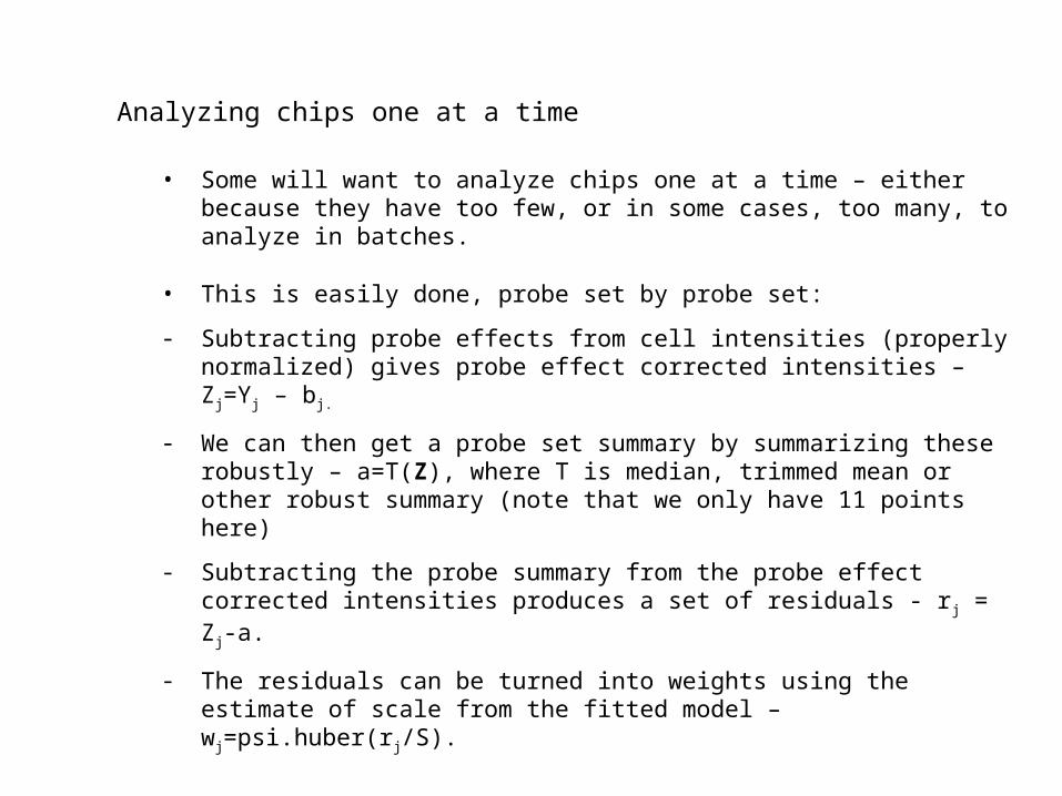
Analyzing chips one at a time

• Some will want to analyze chips one at a time – either because they have too few, or in some cases, too many, to analyze in batches.

• This is easily done, probe set by probe set:

- Subtracting probe effects from cell intensities (properly normalized) gives probe effect corrected intensities – Zj=Yj – bj.

- We can then get a probe set summary by summarizing these robustly – a=T(Z), where T is median, trimmed mean or other robust summary (note that we only have 11 points here)

- Subtracting the probe summary from the probe effect corrected intensities produces a set of residuals - rj = Zj-a.

- The residuals can be turned into weights using the estimate of scale from the fitted model – wj=psi.huber(rj/S).

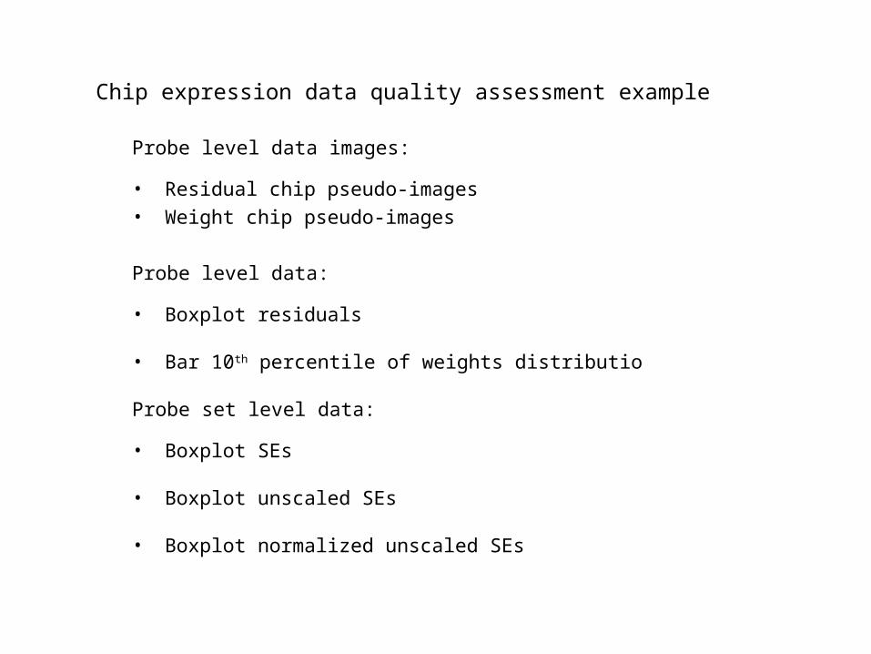
Chip expression data quality assessment example

Probe level data images:

• Residual chip pseudo-images• Weight chip pseudo-images

Probe level data:

• Boxplot residuals

• Bar 10th percentile of weights distributio

Probe set level data:

• Boxplot SEs

• Boxplot unscaled SEs

• Boxplot normalized unscaled SEs

data set used for illustration

• Case study 1 – 24 chips with common pancreas RNA preparation (part of Affymetrix Latin square experiment)

We first look at the RMA derived diagnostics case, by case.

Then look at control and housekeeping genes and 3’-5’ bias, by analysis (to make comparisons between the sources of RNA easier).

Case Study 1 – 24 Chips from Affy Latin square experiment

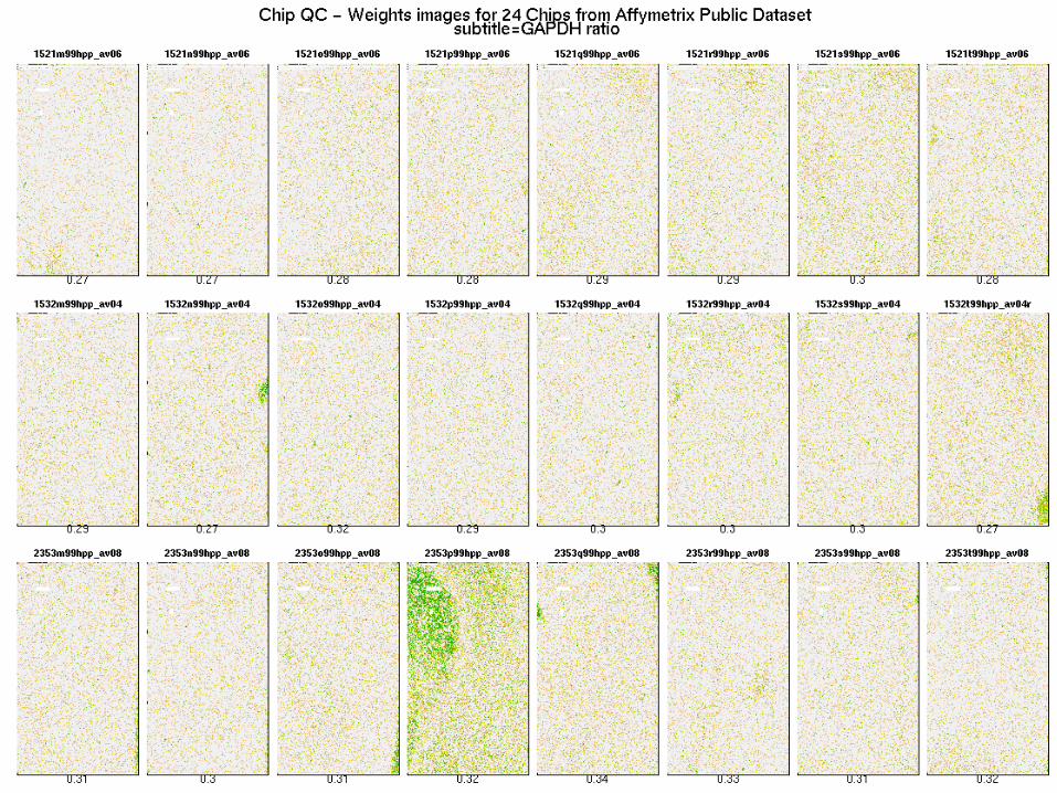
Images of weights

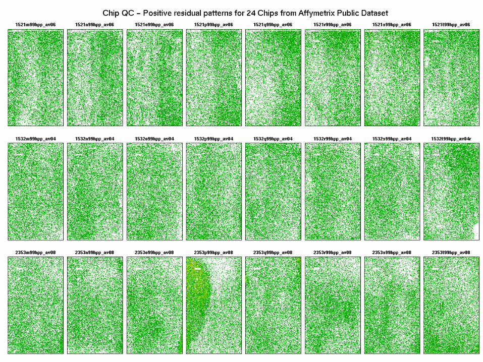
Images of positive residuals

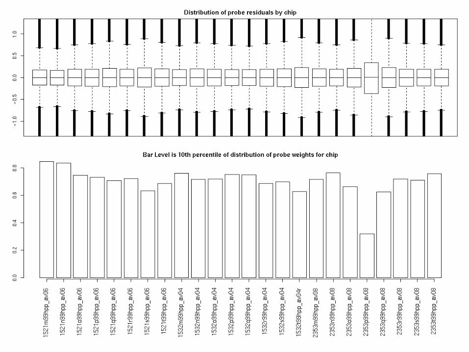
Probe level summaries

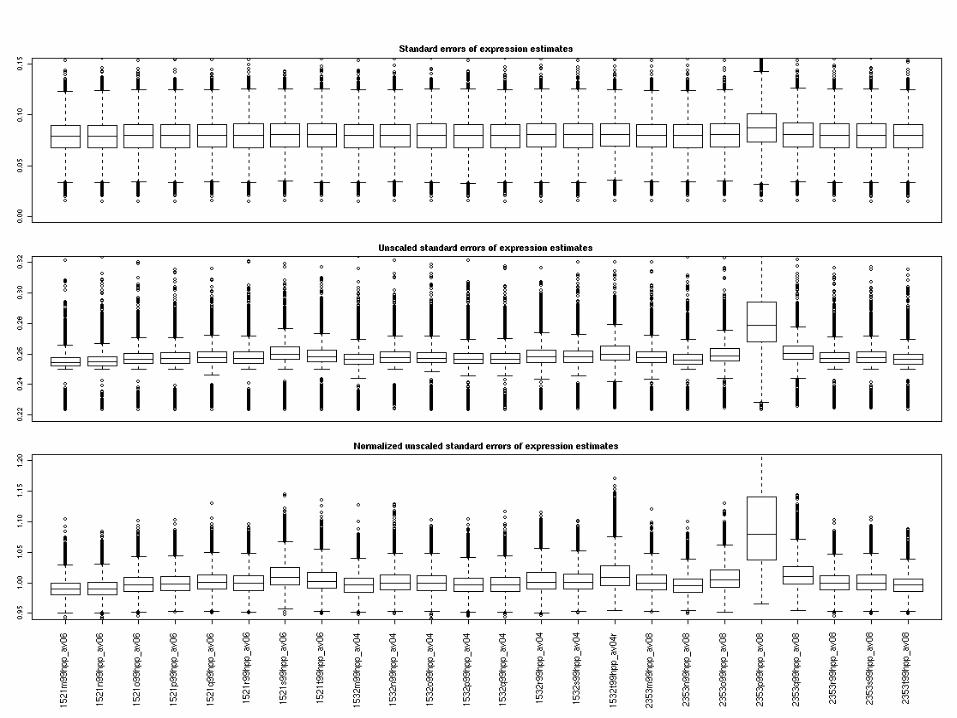
Probe set level summaries

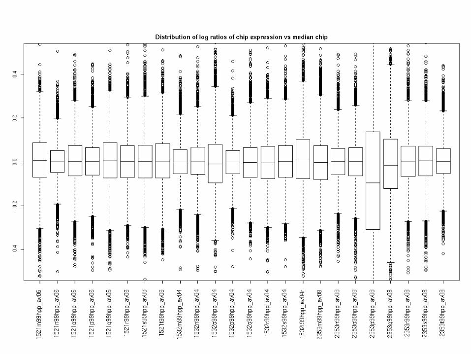
Probe set level summaries - LR

Now look at control/house keeping fragments in Affymetrix chips

• Note that all chips were produced with a common source of RNA. Here look at a sample of 8.

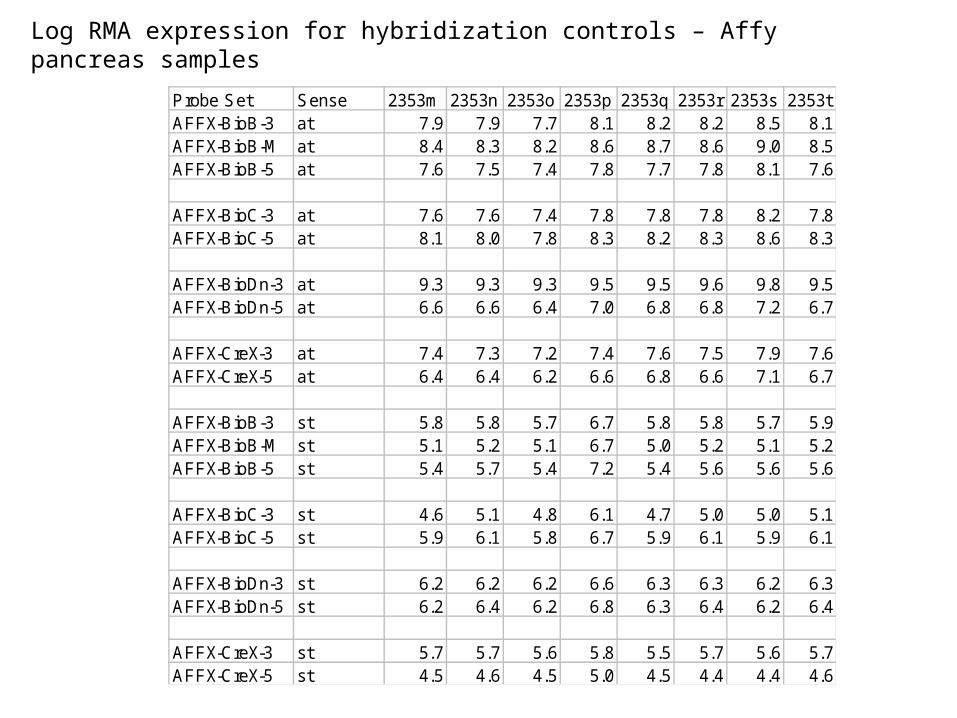
Log RMA expression for hybridization controls – Affy pancreas samples

Probe Set Sense 2353m 2353n 2353o 2353p 2353q 2353r 2353s 2353tAFFX-BioB-3 at 7.9 7.9 7.7 8.1 8.2 8.2 8.5 8.1AFFX-BioB-M at 8.4 8.3 8.2 8.6 8.7 8.6 9.0 8.5AFFX-BioB-5 at 7.6 7.5 7.4 7.8 7.7 7.8 8.1 7.6

AFFX-BioC-3 at 7.6 7.6 7.4 7.8 7.8 7.8 8.2 7.8AFFX-BioC-5 at 8.1 8.0 7.8 8.3 8.2 8.3 8.6 8.3

AFFX-BioDn-3 at 9.3 9.3 9.3 9.5 9.5 9.6 9.8 9.5AFFX-BioDn-5 at 6.6 6.6 6.4 7.0 6.8 6.8 7.2 6.7

AFFX-CreX-3 at 7.4 7.3 7.2 7.4 7.6 7.5 7.9 7.6AFFX-CreX-5 at 6.4 6.4 6.2 6.6 6.8 6.6 7.1 6.7

AFFX-BioB-3 st 5.8 5.8 5.7 6.7 5.8 5.8 5.7 5.9AFFX-BioB-M st 5.1 5.2 5.1 6.7 5.0 5.2 5.1 5.2AFFX-BioB-5 st 5.4 5.7 5.4 7.2 5.4 5.6 5.6 5.6

AFFX-BioC-3 st 4.6 5.1 4.8 6.1 4.7 5.0 5.0 5.1AFFX-BioC-5 st 5.9 6.1 5.8 6.7 5.9 6.1 5.9 6.1

AFFX-BioDn-3 st 6.2 6.2 6.2 6.6 6.3 6.3 6.2 6.3AFFX-BioDn-5 st 6.2 6.4 6.2 6.8 6.3 6.4 6.2 6.4

AFFX-CreX-3 st 5.7 5.7 5.6 5.8 5.5 5.7 5.6 5.7AFFX-CreX-5 st 4.5 4.6 4.5 5.0 4.5 4.4 4.4 4.6

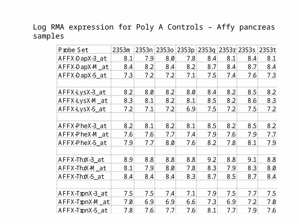
Log RMA expression for Poly A Controls – Affy pancreas samples

Probe Set 2353m 2353n 2353o 2353p 2353q 2353r 2353s 2353tAFFX-DapX-3_at 8.1 7.9 8.0 7.8 8.4 8.1 8.4 8.1AFFX-DapX-M_at 8.4 8.2 8.4 8.2 8.7 8.4 8.7 8.4AFFX-DapX-5_at 7.3 7.2 7.2 7.1 7.5 7.4 7.6 7.3

AFFX-LysX-3_at 8.2 8.0 8.2 8.0 8.4 8.2 8.5 8.2AFFX-LysX-M_at 8.3 8.1 8.2 8.1 8.5 8.2 8.6 8.3AFFX-LysX-5_at 7.2 7.1 7.2 6.9 7.5 7.2 7.5 7.2

AFFX-PheX-3_at 8.2 8.1 8.2 8.1 8.5 8.2 8.5 8.2AFFX-PheX-M_at 7.6 7.6 7.7 7.4 7.9 7.6 7.9 7.7AFFX-PheX-5_at 7.9 7.7 8.0 7.6 8.2 7.8 8.1 7.9

AFFX-ThrX-3_at 8.9 8.8 8.8 8.8 9.2 8.8 9.1 8.8AFFX-ThrX-M_at 8.1 7.9 8.0 7.8 8.3 7.9 8.3 8.0AFFX-ThrX-5_at 8.4 8.4 8.4 8.3 8.7 8.5 8.7 8.4

AFFX-TrpnX-3_at 7.5 7.5 7.4 7.1 7.9 7.5 7.7 7.5AFFX-TrpnX-M_at 7.0 6.9 6.9 6.6 7.3 6.9 7.2 7.0AFFX-TrpnX-5_at 7.8 7.6 7.7 7.6 8.1 7.7 7.9 7.6

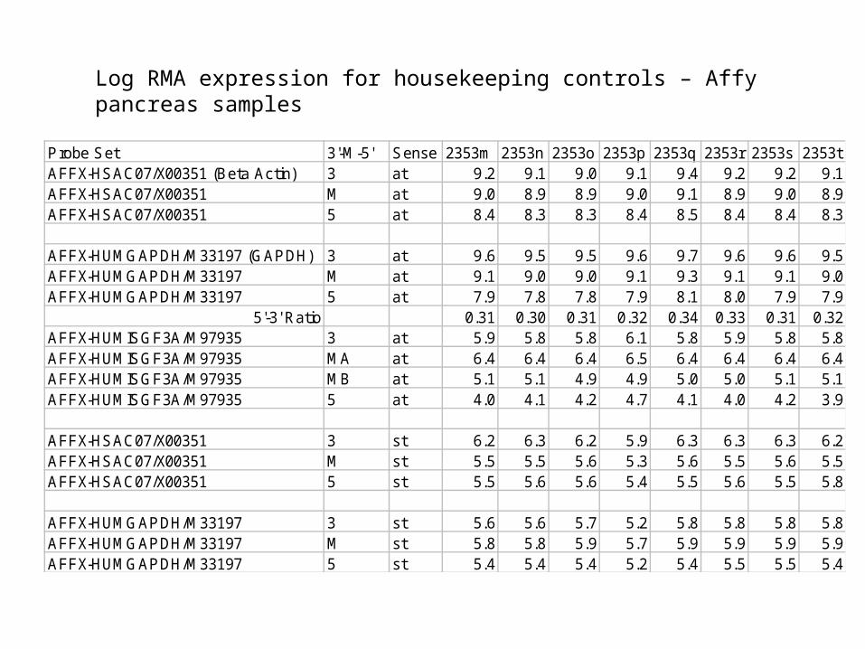
Log RMA expression for housekeeping controls – Affy pancreas samples

Probe Set 3'-M-5' Sense 2353m 2353n 2353o 2353p 2353q 2353r 2353s 2353tAFFX-HSAC07/X00351 (Beta Actin) 3 at 9.2 9.1 9.0 9.1 9.4 9.2 9.2 9.1AFFX-HSAC07/X00351 M at 9.0 8.9 8.9 9.0 9.1 8.9 9.0 8.9AFFX-HSAC07/X00351 5 at 8.4 8.3 8.3 8.4 8.5 8.4 8.4 8.3

AFFX-HUMGAPDH/M33197 (GAPDH) 3 at 9.6 9.5 9.5 9.6 9.7 9.6 9.6 9.5AFFX-HUMGAPDH/M33197 M at 9.1 9.0 9.0 9.1 9.3 9.1 9.1 9.0AFFX-HUMGAPDH/M33197 5 at 7.9 7.8 7.8 7.9 8.1 8.0 7.9 7.9

5'-3' Ratio 0.31 0.30 0.31 0.32 0.34 0.33 0.31 0.32AFFX-HUMISGF3A/M97935 3 at 5.9 5.8 5.8 6.1 5.8 5.9 5.8 5.8AFFX-HUMISGF3A/M97935 MA at 6.4 6.4 6.4 6.5 6.4 6.4 6.4 6.4AFFX-HUMISGF3A/M97935 MB at 5.1 5.1 4.9 4.9 5.0 5.0 5.1 5.1AFFX-HUMISGF3A/M97935 5 at 4.0 4.1 4.2 4.7 4.1 4.0 4.2 3.9

AFFX-HSAC07/X00351 3 st 6.2 6.3 6.2 5.9 6.3 6.3 6.3 6.2AFFX-HSAC07/X00351 M st 5.5 5.5 5.6 5.3 5.6 5.5 5.6 5.5AFFX-HSAC07/X00351 5 st 5.5 5.6 5.6 5.4 5.5 5.6 5.5 5.8

AFFX-HUMGAPDH/M33197 3 st 5.6 5.6 5.7 5.2 5.8 5.8 5.8 5.8AFFX-HUMGAPDH/M33197 M st 5.8 5.8 5.9 5.7 5.9 5.9 5.9 5.9AFFX-HUMGAPDH/M33197 5 st 5.4 5.4 5.4 5.2 5.4 5.5 5.5 5.4

Look at 3’ to 5’ trand in probe intensities over entire chip

• Next slides

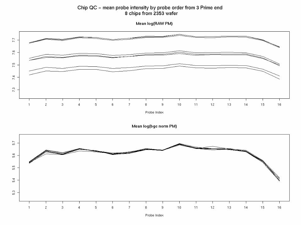
logPM.gc.norm – Affy data

References

1. New Statistical Algorithms for Monitoring Gene Expression on GeneChip® Probe Arrays, Affymetrix technical report.

2. Array Design for the GeneChip® Human Genome U133 Set, Affymetrix technical note.

3. Discussion on Background, Ben Bolstad.

4. Bolstad BM, et. al. (2003), A comparison of normalization methods for high density oligonucleotide array data basedon variance and bias.Bioinformatics. 2003 Jan 22;19(2):185-193.

5. Irizarry, R. et.al (2003) Summaries of Affymetrix GeneChip probe level data, Nucleic Acids Research, 2003, Vol. 31, No. 4 e15 (Available online*)

6. Irizarry, R. et. al. (2003) Exploration, normalization, and summaries of high density oligonucleotide array probe level data. Biostatistics, in press.

7. http://array.mc.vanderbilt.edu/Pages/VMSR_Info/Sample_submission.htm

*http://nar.oupjournals.org/cgi/content/full/31/4/e15?ijkey=EAz2cYYbEWQrE&keytype=ref&siteid=nar