Assessing Damages for the Exxon Valdez Oil Spill

by

Glenn W. Harrison†

February 2006

ABSTRACT

In 1989 the Exxon Valdez ran aground and spilled 11 million gallons of oil in Alaska.Great controversy has surrounded the assessment of monetary damages for this oilspill. The source of this controversy has been the use of hypothetical contingentvaluation surveys to assess damages to individual households, and the aggregation ofthese survey values over all households in the United States. The assessmentprepared for the State of Alaska is reviewed. A number of issues of interpretation ofadvisory survey referenda are raised, each of which could lead to very differentconclusions about the level of damages. The original estimate of $2.8 billion isshown to be highly speculative. True damages could be significantly higher or lower,depending on a priori plausible assumptions required to interpret the surveyresponses. Given the methodological and policy significance of this study, suchinferential uncertainty is unfortunate.

† Professor of Economics, Department of Economics, College of Business Administration,University of Central Florida; GHARRISON@RESEARCH.BUS.UCF.EDU. I am grateful toRichard Carson, Mark Dickie, Shelby Gerking, Michael Hanemann, Bengt Kriström, J.Walter Milon, Elisabet Rutström and V. Kerry Smith for conversations and healthy debate.Supporting data are stored at http://exlab.bus.ucf.edu.

1 A shortened version of the full report was published as Carson et al. [2003].

- 1 -

On March 24, 1989, the Exxon Valdez ran aground on Bligh Reef and spilled about 11

million gallons of oil into Prince William Sound. The oil spill eventually spread over 10,000 square

miles of water and 1,000 miles of shoreline. Most of the damage occurred in Prince William Sound

and the Gulf of Alaska. It was immediately apparent that the Exxon Valdez oil spill was a major

environmental catastrophe: physical injury to the environment was grave.

Within weeks of the spill a number of academics and consultants were contacted to propose

studies of the damage assessment in economic terms. For the Attorney-General of the State of

Alaska, the primary trustee in the case, Carson et al. [1992] were contracted to undertake the

assessment of damages.1 For the Federal trustees Allan Randall was retained, but no report was ever

released. Exxon, the primary defendant in the case, retained Bill Desvousges. Apparently no survey

was ever conducted by the Exxon team pertaining directly to the Exxon Valdez oil spill, although

that strikes many as simply incredible given the nature of the litigation and the stakes involved.

The contingent valuation method (CVM) was employed by Carson et al. [1992] to assess

damages. Their CVM study, the Exxon Valdez study for short, has significantly impacted the way in

which CVM studies are viewed, evaluated, and proposed. There is no doubt that in many respects it

represents a state of the art assessment, using methods that have been refined over many years on

studies of smaller environmental injuries.

The Exxon Valdez study estimated a median willingness to pay for a spill prevention plan to

be approximately $31 per household. Multiplying this median by an adjusted number of U.S.

households results in an aggregate damage assessment of $2.8 billion. This estimate was the bottom

line of the CVM study conducted by Carson et al. [1992].

The main conclusion from an evaluation of the Exxon Valdez study is that the estimates are

2 There is controversy concerning the implications of the use of hypothetical valuation questions inenvironmental damage assessments. Controlled laboratory evidence demonstrates that significant hypothetical bias existsin these responses. This evidence pertains to simple open ended elicitation methods (Neill et at al. [1994]), simpledichotomous choice valuation questions for private goods (Cummings, Harrison and Rutström [1995]), and binarychoice referendum questions (Cummings, Elliott, Harrison and Murphy [1997]). These studies indicate that hypotheticalbias can result in a significant upward bias in the results of CVM surveys. Although there exists constructive methods formitigating the extent of hypothetical bias, these methods are currently exploratory and have not been applied in the field(see Harrison [2004] for a review). For the purposes of this study we do not directly question the CVM study on the grounds ofhypothetical bias. This is not to ignore this problem, but simply to recognize that it must be dealt with separately from thehost of problems that confront a CVM researcher.

3 The settlement was accepted on October 9, 1991 by the U.S. District Court. Exxon agreed to pay a criminalfine of $150 million, $125 of which was forgiven in recognition of Exxon’s clean-up efforts ($12 million of the remaining$25 million went to the North American Wetlands Conservation Fund, and $13 million to the national Victims of CrimeFund). Exxon also agreed to pay $100 million to the trustees as criminal restitution for the injuries caused to fish, wildlifeand land. Finally, Exxon agreed to pay $900 million to the trustees over a 10-year period to settle the civil actions. Thesettlement allowed for a possible additional $100 million in damages if resource damage occurred that could not havebeen anticipated at the time of the settlement.

- 2 -

extremely sensitive to how they are interpreted. Even if one believes that the CVM study does not

suffer from any intrinsic biases due to the hypothetical nature of the key valuation question,2 it is still

apparent that the $2.8 billion estimate is a speculative assessment of the true damages caused by the

Exxon Valdez grounding. The primary issue of interpretation is whether the responses should be

taken “literally” or as the basic for identifying some “latent” population value.

The actual damage award, in the case of the Exxon Valdez, deviated significantly from the

award that would have been predicted on the basis of the CVM study. While the CVM study

provided a best guess estimate of $2.8 billion in compensatory damages for the oil spill, the actual

settlement was $1.025 billion.3 Although the final report of the CVM study was written subsequent

to the actual damage assessment, and may have been influenced in some respects by an attempt to

validate the actual damage award, we must assume that it was an honest attempt to estimate for the

state trustees the true damages of the Exxon Valdez oil spill. We evaluate it on that basis, knowing

that there were in fact many political considerations relevant to the design and presentation of the

report in public form. If the CVM study is to be considered as a scientific document on its merit, no

other perspective is possible.

A closely related CVM study of the Kakadu Conservation Zone in Australia is described by

4 I am particularly grateful to V. Kerry Smith for making these data available, along with documentation. Datafrom the original study were generously made available by Richard Carson in April 2004. Their distribution prior to thatdate had apparently been restricted by the sponsoring government agency. The raw data from the original study cannotbe found on the web site listed by Carson et al. [2003; p.281, fn.9], although it is available at http://exlab.bus.ucf.edu.

- 3 -

Carson [1992] and Carson, Wilks and Imber [1994]. Many conceptual issues that arose with the

Exxon Valdez study also arise with the Kakadu study, and both are considered since these issues

attracted more written, public debate in the Kakadu study.

In 1993 a replication and extension of the ExxonValdez oil spill survey was conducted. The

replication was close, in the sense that essentially the same survey instrument was used from the

original study and the same in-person survey method used. Results from the 1993 replication were

published in Carson et al. [1998] and Krosnick et al. [2002]. Although the raw responses from the

original Exxon Valdez CVM study have not been available for public review until very recently, the

responses from the 1993 replication have been available.4

In section 1 we briefly review the main features of the Exxon Valdez CVM study: the

development of the survey instrument, the final questionnaire, the survey administration, and the

statistical analysis. In section 2 we address several problems with the study. These problems are the

use of the median rather than the mean to infer aggregate damages, the way in which the mean was

calculated, and ambiguities in the scenario specification. In section 3 we consider a deeper question

concerning the appropriate interpretation of “advisory” survey referenda. In section 4 we offer an

overall assessment of the damages calculated for the oil spill.

There is little doubt that the academic debates over the validity and reliability of the CVM

have been at cross-purposes. This was the clear, adversarial objective of the Exxon-commissioned

studies collected by Hausman [2003], which defined the nadir point of the academic debate. Nor did

the assertive tone of the NOAA Panel report by Arrow et al. [1993] help matters. Finally, the

productive debates generated by controlled laboratory and field experiments, reviewed by Harrison

- 4 -

[2006], have obviously limited applicability to broader natural contexts in which CV is applied. What

is needed is a focus on substantive issues that arise in a specific policy application that avoids

obvious constraints in implementation. Thus one has to agree with Carson et al. [1993; p. 259] on

the signal importance of the Exxon Valdez study:

The results of the CV study conducted for the State of Alaska in preparation for the Exxon Valdezlitigation presented here represented the contemporary state-of-the-art, and therefore, stands as areference point that may be used to assess the criticisms of CV and perhaps the more general debatesurrounding passive use. Most of the recommendations made by the NOAA panel to help insure thereliability of CV estimates of lost passive use had already been implemented in the Alaska study [...] Asmuch of the debate focuses on old CV studies, or small experiments, a reference point portraying CVpractice when substantial resources were available to undertake the study should enhance the quality ofthe debate.

1. Review of the Exxon Valdez Study

A. Survey Development

The survey was developed from July 1989 until January 1991, when the final survey

instrument was taken into the field. This is clearly a slow process, but is one that is regarded by

CVM researchers as critical to the generation of a survey instrument that one can have confidence

in. Although it is natural for economists with little experience in survey development to skip over

the description of how the survey instrument was developed, a brief review of the procedures and

steps taken will provide useful background to help evaluate the final decisions embodied in the

instrument taken into the field.

The essential steps in the survey development were a series of focus groups. The initial focus

groups consisted of about seven groups with roughly ten people per group. These individuals were

paid to attend the meeting and discuss the issue and difficulties with alternative formulations of the

problem. They were typically conducted as open ended interview sessions where the subjects may

have been guided by an interviewer trained to elicit their responses to a series of questions germane

to the design of the instrument.

- 5 -

Initial Design Choices

As a result of these initial focus group sessions, a series of initial design choices were made in

the survey instrument. These initial design choices are of some importance for the sequential

revision of the survey instrument that took place during the process of survey development.

The first design choice was to propose a scenario for consideration by subjects that

consisted of the provision of an escort ship for tankers departing from the Port of Valdez. This

escort ship would assist the tanker in navigating the waters of Prince William Sound, and would

leave the ship once it was in open seas. An additional component of the scenario was the provision

of Norwegian sea nets, which are a popular method for containing oil spills in relatively calm waters.

The idea is to surround the stricken vessel with sea nets that are partially submerged, hoping that the

sea nets can contain the oil spill before it disperses. While the sea nets would contain the oil, tankers

would be requested to come to the spill site and remove the oil from the contained area within the

sea nets. A final component of the scenario was the statement that legislation implementing double

hull laws would be enacted within ten years that would ensure safety with respect to incidents such

as the Exxon Valdez. In essential respects the scenario did not change during the survey

development, although presumably the precise set of words and the manner in which it was

explained to subjects did change.

Another initial design choice of some significance was the use of double bounded

dichotomous choice (DC) questions. A double bounded DC question proceeds by asking the subject

if they are willing to pay an initial price. The initial DC prices used were $10, $30, $60 and $100, with

follow up prices as high as $250. For example, if a subject was asked initially if they were willing to

pay $10 and they said yes, there would be a follow up question asking if the subject would then be

willing to pay $30. If the subject said “no” to a request to pay $10, the follow up question would be

$5.

- 6 -

A third initial design choice was the use of a payment vehicle by which individuals would pay

the higher oil prices and that there would be no oil company share in the amount contributed

towards this scenario.

The final key design choice was to have subjects pay over ten years in multiple payments.

These payments would be one per year for a constant amount over ten years.

Sequential Design Choices

The first full-blown pilot survey consisted of 105 respondents. It resulted in several changes

to the instrument. First, there were many minor revisions in the choice of words and phrasing, as

expected. A major problem with the credibility of the multiple year payment was encountered,

resulting in a focus group on the credibility of multiple year payments with respect to consumer

durables. A 500 person phone survey was also undertaken, directly comparing lump sum payments

versus multi-year payments for a scrubber to be added to a polluting factory.

A decision was made to adopt the lump sum payment for enhanced credibility, as well as

being “conservative.” The term conservative appears throughout the design stages of the instrument

and is worth defining explicitly. In the present context it simply means biased-down. The term is

used in other disciplines, such as accounting and political science, but the meaning here is that the

instrument is called conservative if it results in an estimate that is biased-down relative to the

expectation of a true or alternative estimate. Since the variants of the wording of the hypothetical

survey instrument do not provide evidence of a true willingness to pay, in the sense of a real

economic payment elicited under demand revealing circumstances, the term conservative in practice

is used here to mean any design choice which results in an estimate that is smaller than an alternative

design choice.

A second pilot, consisting of 195 respondents, was also conducted and resulted in several

- 7 -

important tests. The first was a test of the payment vehicle, in which the survey compared the effects

of either having a tax payment by oil companies and respondents, or a surcharge that would only be

imposed on oil companies (resulting in higher oil prices). A split sample was adopted for each of the

alternative tax payment vehicles. The result was a higher willingness to pay with the surcharge

vehicle and few protests since oil companies now paid a share.

A third pilot consisted of 244 respondents. It employed a slight rewording of the surcharge

payment vehicle and another split sample design to re-examine the alternative tax payment vehicles.

The result was that there was no difference in willingness to pay. By design this sample used a much

poorer and lower educated group, to presumably test if the basic wording of the scenario would be

adequate for this strata of the population. At this point it was decided to use the tax vehicle, mainly

due to the instability of oil prices, resulting in subjects having difficulty understanding the size of the

payment required relative to then-recent changes in oil prices (this was the period of the Iraqi

invasion of Kuwait). An additional consideration in favor of the tax vehicle was that the second pilot

suggested it to be the conservative choice, in the sense of resulting in a smaller willingness to pay.

A fourth pilot consisting of 176 respondents entailed minor changes in maps and wording,

and was viewed as a final test run for the instrument. In this pilot survey the upper initial DC price

was $150 instead of $100. The final decision was to use $120 as the highest initial DC price,

although there is no discussion of the reason for this final decision. Indeed there was surprisingly

little discussion throughout the survey development of the use of alternative DC prices.

B. The Final Questionnaire

The final questionnaire consisted of several stages. The first part had a number of general

attitudinal questions, designed to “warm up” the subjects by having them answer some non-

controversial questions. The second part of the questionnaire tested the knowledge that the subject

- 8 -

had of oil spills. The third part of the question provided information specifically on the Exxon

Valdez oil spill. This stage provided many maps and pictures explaining the point of origin of the

spill and the dispersal of the oil slick. It provided a clear statement that no species were threatened

with extinction despite heavy losses in absolute terms for some species such as murres. It mentioned

Exxon’s cleanup efforts. It also provided a discussion of the transitory nature of most of the

environmental injury.

The evaluation scenario was presented largely in terms that were chosen in the initial design

stage. The scenario asked subjects to consider willingness to pay for an escort ship and an

emergency Norwegian sea net program. The subjects were told that until double hulling laws take

effect in ten years they were to expect another large oil spill in Prince William Sound of the same

size and potential scope as the Exxon Valdez oil spill. The escort ship and sea net scenario was

presented as a way of reducing the chance of such an oil spill effectively to zero during the next ten

years, upon which time the double hulling laws would presumably reduce the probability to zero.

The key valuation question embodied several of the design features that were initially

adopted. Subjects were asked their willingness to pay a one time tax on Alaskan oil companies and

citizens. Reasons were given why the subject might vote “yes” and might vote no; indeed, these

reasons were remarkably honest and quite extensive. Subjects were told that the final cost had been

estimated for their household to be X dollars. If the subject said that they would be willing to pay X

dollars they were then asked if they would be willing to pay if the final cost for their household

actually was Y dollars, where Y is greater than X. If the subject said that they would not be willing to

pay X dollars, the follow up question asked if they would be willing to pay if the final cost was

actually Z dollars, where Z is less than X. The values of X, Y and Z used in the survey are illustrated

in Table 1, along with the implied interval responses for the four possible responses to these two

questions.

- 9 -

The questionnaire then provided some follow up questions to help understand the subjects’

response and assess beliefs about the scenario as presented. A series of questions asked households

about their social and demographic characteristics. Subjects were asked to then state the strength of

their voting intention and the possibility that they would revise their response. Subjects were also

given the opportunity to actually go back and revise their response. Finally, there was an extensive

interviewer debriefing in which the interviewer was asked to describe the nature of the interview and

the extent to which the subject was attending to the presentation and seemed to take the evaluation

questions seriously. This debriefing occurred after the interviewer had left the house of the subject.

C. Survey Administration

The survey was national in scope, since it was attempting to estimate passive or non-use

values from the Exxon Valdez oil spill. The trustees for the area affected by the oil spill were charged

with representing the interests of all United States adult citizens, so it was appropriate from a legal

perspective to assess damages over such a wide group. This was also appropriate given the scope

and importance of the injury, not to mention the press that it received on national television and

other media.

A second feature of the survey administration is that the survey was conducted in person,

with an interviewer receiving extensive training and actually visiting the residence of the respondent.

The sample was stratified, so as to represent the adult United States population. The stratification

procedure required that one identify a number of characteristics of the population that the sample

should represent. These characteristics were region, age, race, household size and marital status.

Based on these stratification variables, and knowledge of the population weights for each strata,

sample weights were constructed. The report is not specific as to the importance of these weights,

other than to say (p. 97, fn. 83) that their use does not change the main conclusions.

5 The settlement of the litigation led to the reduction in the final sample size.

- 10 -

An English language version of the instrument was developed. The cost of developing a

Spanish version was deemed to be prohibitive and costly. No sample correction was made for the

lack of a Spanish version, but the target population was reduced by 2.7 percent so as to reflect the

English speaking population in the United States. The target population was taken to be 90.838

million households, to represent the adult United States population.

Although the original plans called for roughly 2,000 completed surveys, eventually 1,043

surveys were completed based on 1,599 households drawn or sampling.5 Hence the response rate is

roughly 75%, a good response rate by any standards. The cost of a completed survey rose

considerably during the administration of the survey, from roughly $50 up to $600 per completed

survey near the end, due to the need to make several visits to some respondents in order to insure

that they were in the sample.

D. Survey Analysis

The analysis in the report contains an excruciatingly boring discussion of the attitudinal

responses. The meaty analysis begins with an examination of the first evaluation question (A-15).

Table 2 reports the raw responses to this question. In the survey responses are categorized as “yes,”

“no,” or “not sure.” Consistent with past practice, and consistent with the implied contractual

counterpart of this question, we group the “no” and “not sure” responses together in Table 1 unless

otherwise specified. This is consistent with the notion that if a subject did not say “yes” then there is

no presumption that the subject would actually pay the amount of money, even in the hypothetical

legal setting. Formalizing this intuition, Harrison and Kriström [1996] propose that we interpret DC

responses as a “minimum legal WTP” since the subject has only said “yes” to the amount asked,

6 In part this unfortunate inferential outcome is due to the use of large, discrete intervals for the DC prices, andthe use of the same intervals for each subject in each version. It would be a simple matter to employ a random shift inDC prices for each subject, to ensure even coverage of interim DC prices.

- 11 -

even if they might be willing to pay a higher amount if asked.

The most important feature of these raw responses to the first evaluation question is the

speed at which the percent “yes” responses decline as the price increases. Table 1 shows that 67% of

the sample said “yes,” indicating that they would be willing to pay $10, and that this percentage

dropped to 52% or 51% as the price increased to $30 or $60. It further decreased to 34% as the

price increased to $120. There is no significant decline in the percent “yes” response as we move

from $30 up to $60.

If the objective is to infer the DC price at which 50% of the sample is willing to pay for the

project, then there is considerable uncertainty whether the true responses lie between $30 and $60.

Indeed one might say that there is comparable uncertainty about responses for values slightly less

than $30 or slightly greater than $60, since we do not know at precisely which point the response

rate of 67% at $10 declines to a 52% response rate at $30. It is possible that at $11 all subjects would

respond “yes” with a probability of .52 and that this response rate holds constant up to the price of

$30. It is clear that we are just speculating at this point, but it is apparent already that the use of some

parametric assumptions in the subsequent statistical analysis will be crucial in arriving at estimates of

a precise median or mean willingness to pay for each household.6

The responses to the double bounded questions (A-15, A-16 and A-17 in the survey) result

in the classification and response rates indicated in Table 2. These responses can be compared to the

implied intervals in Table 1. Thus we see that a “yes,” “yes” response in survey version A implies

that the subject is willing to pay any amount from $30 up to infinity, and from Table 2 we see that

45% of the survey A respondents fall into that category. A critical issue in the statistical analysis of

this type of DC data is the speed with which the “yes” responses decline in the right hand tail,

7 The term “survival” comes from the original use of these models to study how long subjects survived aftermedical treatment. In the present application the amount the subject is willing to pay is the same as the survival time. Ofcourse, this interpretation plays no role in the formal statistical analysis or the calculation of damages. These models arealso referred to in the labor economics literature as “duration models,” since time can also be viewed as a duration.

- 12 -

corresponding to latent valuations that are arbitrarily large. If this tail does not decline reasonably

rapidly then the resulting mean estimate is likely to be very large indeed, as high willingness to pay

values are included even if they occur with a low probability. Thus it is of some comfort to notice a

steady and monotonic decline in the “yes,” “yes” responses as we proceed from survey Version A

through Version D. Only 14% of the respondents that were asked implicitly if they were willing to

pay greater than $250 said “yes”. Hence only 14% of the respondents are left in this open interval.

When parametric functional forms are used to fit the data over the complete range of

willingness to pay, responses that are only known to be “greater than $250” can have a significant

impact on estimates of willingness to pay that are much lower. Thus it is not appropriate to say that

one does not care about the responses to high willingness to pay numbers if parametric functional

assumptions are being used in the subsequent analysis.

The first approach to valuation in the report is non-parametric, using an estimator referred

to as the “Turnbull estimator” after Turnbull [1974]. This approach ignores the socioeconomic

characteristics of the sample, implicitly assuming that the sample is representative of the population.

The non-parametric approach that is used is a standard one for interval-censored data of this kind,

and is used to estimate a median interval and a mean interval. Given the uniformity of response

between the $30 to $60 interval, it should come as no surprise that there is a relatively wide interval

obtained by the non-parametric approach.

The second approach to estimation in the report is parametric, using an estimator referred to

as a “Weibull survival model.” This approach can incorporate the socioeconomic characteristics of

the sample, and is relatively flexible within the class of survival models.7

8 The “population” refers to those individuals that have legal standing in the matter. Typically this will be theadult citizens of one country. It could also be defined on a household basis.

9 The same sort of comparison can be made for the Kakadu study documented by Imber, Stevenson and Wilks[1991]. Their preferred median estimate (p. 75) for the Minor impact was $52.80 per person per year for ten years (p. 76),resulting in an aggregate annual damage estimate of A$647 million. This point estimate of the median, however, isderived by linear interpolation of a non-parametrically estimated interval, and has little to recommend it statistically(Carson [1991b; p. 46]). Using the preferred parametric estimates from their Weibull duration model (p.87), one obtains a

- 13 -

2. Critique of the Exxon Valdez Study

A. Mean Versus Median

The goal of most environmental damage assessment exercises is to assess aggregate damages

resulting from some environmental insult, such as an oil spill or mining activity. This measure of

aggregate damage to the population8 could be used to assess a fine against some liable party or to

assess gross benefits in a cost-benefit analysis for some government agency.

In order to assess aggregate damages, without having to sample the entire population, one

can proceed by generating an estimate of the population mean WTP. This estimate may then be used

to infer aggregate damages by just multiplying it by the number of households or individuals in the

population.

For skewed distributions, the median and the mean will typically differ. In the case of WTP

responses in CVM surveys, the problem is one of right-skewness, with a large number of people

being willing to pay small amounts of money and some saying that they are willing to pay a very

large amount of money. In such a setting the median is invariably much smaller than the mean.

In the Exxon Valdez study, for example, the preferred estimation procedure generated a

median WTP of $31 and a mean WTP of $94 (Table 5.8, p. 99, using the Weibull distribution).

Multiplying the median by the number of English-speaking households, estimated in the study to be

90.838 million (p. 77-78), one obtains the preferred estimate of aggregate damages of $2.816 billion

(p. 123). If the mean had been used instead, this aggregate damage estimate would have been $8.539

billion.9 A big difference, particularly if you are the one writing the check!

median point estimate of $80.30 (p. 76) and a mean point estimate of $1931.46 (p. 86). These result in annual damageestimates of $985 million and $23,682 million, respectively.

10 The location parameter is just the mean of the distribution, and the scale parameter the variance.

- 14 -

How, then, is the exclusive use of the median justified? The arguments in the Exxon Valdez

and Kakadu studies are slightly different in this respect. Since their statistical design is so similar, but

their assessment goals were instructively different, we review both sets of arguments.

The Valdez Argument

The argument in the Exxon Valdez report is that the median is to be preferred (i) since “...

the mean can not be reliably estimated and the median can be reliably estimated” (p. 101), and (ii)

the median is a “... lower bound for the damage estimate” (p. 11) since the median is smaller than

the mean.

The argument that the mean cannot be reliably estimated runs as follows. Using four

alternative distributional assumptions, a regression model is developed to explain WTP responses as

a function of a “location parameter” and a “scale parameter.”10 No covariates, to reflect the possible

effect of explanatory variables such as respondent age or sex, are used. The model is estimated by

maximum-likelihood procedures, and the resulting means and medians from the estimated model are

tabulated. For the Weibull, Exponential, Log-Normal, and Log-Logistic models, the medians are

found to be $31, $46, $27 and $29, and the means to be $94, $67, $220 and infinity, respectively

(Table 5.8, p. 99).

It is possible to discriminate between these distributions statistically. For example, the

Exponential is a special case of the Weibull. This leads (p. 100) to the rejection of the Exponential

distribution using standard tests. Although the Log-Logistic and Log-Normal are not special cases of

the Weibull, a non-nested test leads to the rejection of the Log-Logistic in favor of the Weibull (p.

101, fn. 85). It was not possible to discriminate, however, between the Weibull and Log-Normal

- 15 -

distributions using this non-nested test. The argument for using the Weibull distribution as the

preferred alternative between the two “survivors” seems to be that it is the most popular (p. 97) and

is flexible with respect to the representation of WTP responses (p. 98).

The estimate of the mean is then deemed unreliable since “... the shape of the right tail of

the chosen distribution, rather than the actual data, is the primary determinant of the estimate of the

mean.” (p. 101, footnote omitted). This is illustrated by the variability of the mean estimates listed

above over the four alternative distributions. However, the previous argument had just eliminated all

but two of these distributions on statistical grounds: only the Weibull and Log-Normal remain as

viable candidates. Hence there are just two alternative estimates of the mean to be considered, one at

$94 and the other at $220 (the latter resulting in an aggregate damage amount of $20.711 billion).

Moreover, the informal grounds for preferring the Weibull over the Log-Normal should apply here

as well, suggesting that there is some basis for just preferring one distributional assumption, the

Weibull, and its estimates of median and mean.

Thus there appears to be no consistent statistical basis in this line of argument for

eliminating the mean from consideration. The arguments advanced for eliminating all but the

Weibull distribution with respect to the use of the median apply equally to the use of the mean, since

they were not couched with reference to the use of the median or the mean.

Consider now the argument that the median is to be preferred since it is smaller than the

mean, and hence provides a more “conservative” measure of aggregate damages. This line of

argument has become popular, and appears in the findings of the CVM Panel of the National

Oceanic and Atmospheric Administration, Arrow et al. [1993; p.4608], as follows:

Generally, when aspects of the survey design and the analysis of the responses are ambiguous, the optionthat tends to underestimate willingness to pay is preferred. A conservative design increases the reliabilityof the estimate by eliminating extreme responses that can enlarge estimated values wildly and implausibly.

The same argument appears throughout the Exxon Valdez report (e.g., pp. 11, 30, 33, 112-117).

- 16 -

The problem with this argument is that it begs the reason that we want to bias the estimates

in the first place. It is obvious that the reason that the Exxon Valdez study wants to do so is to be

able to justify a fine of at least $2.8 billion. The authors of that report clearly want the reader to come

away with the impression that the true level of aggregate damages is above that figure, and that there

is very little chance of the true level of aggregate damages being less. Nonetheless, the argument for

a “conservative” lower-bound choice of the median would only appear to hold water when there is

some ambiguity as to whether the mean or the median should be used. No such ambiguity has been

articulated in the Exxon Valdez report, suggesting that their application of the “be conservative”

guideline is actually inappropriate in this instance.

The Kakadu Argument

The Kakadu study recognizes that the mean is the logically correct estimate for use in cost-

benefit analysis (p. 82-83), but opts for the median on two grounds. The first is that it ignores

distributional considerations, and the second is a variant on the “statistical reliability” argument

discussed above.

The discussion of distributional concerns does point the way to a proper conceptual basis

for discriminating between mean and median due to Johansson, Kriström, and Mäler [1989] and

Hanemann [1989]. The report begins by arguing that the mean has the “... disadvantage that the

distributional consequences of the policy in question are not addressed by use of the mean. The

result is that a benefit-cost analysis will be weighted towards the relative valuations of the wealthy.”

(p. 82) On the other hand, the DC approach “... can take account of the distributional desires of the

electorate by eliciting the tax payment that half of the electorate is prepared to make. The most

useful policy interpretation of the results of this survey is therefore likely to be to use the median

result in a referendum framework. This prevents the result from being too strongly influenced one

11 It is relatively easy within a numerical general equilibrium framework to take into account the effects of actualsidepayments on relative prices and hence the welfare evaluation that gave rise to them. It is common in such settings tocalculate the smallest aggregate set of sidepayments that ensure that there are no losers, allowing for the feedback effectsof the sidepayments. See Harrison, Jensen, Lau and Rutherford [2001] and Harrison, Rutherford and Tarr [2003] forpolicy illustrations. For small, local economies, such as Alaska, it is likely that these general equilibrium effects could beimportant enough to have to allow for.

- 17 -

way or another by the desires of a few.” (p. 82).

These arguments simply do not make much sense. Consider a project that generates gross

benefits of $1 to each of two people and $100 to a third. If the gross cost of the project is $4, then

social welfare depends on how the costs are distributed and on the particular social welfare function

(SWF) adopted.

If the costs are distributed equally between the three, then a Rawlsian SWF would judge this

project as not being worth pursuing since at least one member of society is made worse off (in fact,

two are). Similarly, a Majority Rule SWF would decide against it. On the other hand, a Utilitarian

SWF would judge this project as being worthy since the sum of the net benefits to society are

positive. Assuming away any general equilibrium effects from redistribution, the same conclusion

would obtain from the joint use of a Kaldor-Hicks SWF and the Pareto Criterion (assuming

hypothetical sidepayments), or directly from the Pareto Criterion viewed as a SWF (assuming actual

sidepayments).11

The issue then becomes the relative plausibility of these alternative SWF assumptions. If the

Majority Rule SWF is deemed appropriate, then the median will tell us what we need to know since

it will be the median voter who decides the issue in a single-dimension case such as considered here.

If the Utilitarian SWF, Kaldor-Hicks SWF or the Pareto SWF are deemed appropriate, then the

mean will tell us what we need to know.

There is no basis for asserting the primacy of one SWF over another in all circumstances. As

Hanemann [1991; p. 188] notes in the context of the Kakadu study, “I personally find the Kaldor-

12 The only other place is in reference to the use of DC questions: “... if dichotomous valuation questions areused (e.g., hypothetical referenda), separate valuation amounts must be asked of random sub-samples and theseresponses must be unscrambled econometrically to estimate the underlying population mean or median.” (p. 4611).

13 One is unlikely to see this argument advanced by a critic of the CVM hired by a defendant, since it might beseen as arguing for a higher damage estimate. This is unfortunate and myopic of the CVM critics, since it arguably pointsto deeper concerns with the validity of the CVM. Mead [1993] presents a version of this Laugh Test, but in such anunbalanced and snide manner as to not warrant further scholarly attention.

- 18 -

Hicks criterion unattractive in many cases, and I don’t believe that it automatically governs all cost-

benefit exercises.” This suggests that he would opt for the median. On the other hand, we find the

Pareto SWF, assuming actual sidepayments such that real income is no lower for any household than

before, to be attractive, and would opt for the mean. The reason is that the objective of the analysis

is to calculate compensatory damages, and to make all parties “whole again” one must generate

enough money to fully compensate each and every injured party. To adjust the previous example, if

two individuals required $1 each to be compensated, and one individual required $100, we would

have to raise $102 in total.

The NOAA [1993] Panel is silent on this issue, although in virtually12 the only place that it

mentions either of the words “median” or “mean,” it claims that a “... CVM study seeks to find the

average willingness to pay for a specific environmental improvement.” (p. 4606; emphasis added).

This suggests the implicit adoption of the Kaldor-Hicks or Pareto SWF, or perhaps even the

Utilitarian SWF. Existing CVM studies do not elicit the preferred form of the SWF, although it

could readily be done.

An Assessment

One concern that appears to underlie the arguments in favor of the median in these two

reports is a fear that the mean just will not pass the Laugh Test. In other words, the values for the

population mean implied by the way WTP responses are modeled are just too high to be plausible.13

Rather than being ad hoc, this line of argument is eminently sensible and reflects the use of a priori

14 See Harrison [2006] for further discussion of procedures to detect and mitigate hypothetical bias.

- 19 -

beliefs about the process being studied. What is necessary, however, is that one not apply incorrect

arguments to defend this proper Bayesian exercise. Instead, the confusion over “mean versus

median” reflects two more fundamental sources of discomfort with the results of CVM studies, and

one ought to address these issues first and foremost instead of dancing around them.

The first issue is the appropriate way to view the tax-price that is offered in a CVM. We

argue in the next section that it should be viewed as defining an implicit contract between two

agents, typically the government and the population. This has an important implication for how DC

responses ought to be interpreted in statistical analyses. In Section 3 these concerns are expanded to

take into account the possibility that the survey respondents choose not to vote at all.

The second issue is the validity of using a hypothetical WTP to effect real economic

payments, either in the form of fines or in the form of allocated resources for some project (that

passes a cost-benefit test that uses the CVM). We believe that CVM researchers ought to focus

considerable effort on this issue, but say nothing more here.14

B. Estimating Mean WTP

Assuming that one should be measuring mean WTP rather than median WTP, how should it

be done? Harrison and Kriström [1995] propose using an estimator that they call the Minimum

Legal Willingness to Pay (mlWTP). The motivation for the mlWTP estimator is that one recognizes

that these estimates are being prepared in the context of litigation, and typically for use by a jury of

non-specialists. Hence the estimator should have two properties: admissibility and transparency.

The notion of admissibility concerns the type of evidence that can be entered in a court-

room, and the factual basis of that evidence. If some witness is a “fact witness” then they can only

- 20 -

testify as to things that they know to be true. Hearsay is therefore not admissible for a fact witness,

since they do not know that the statement about a third person’s actions is factually correct. But if

some witness is designated as an “expert witness,” the standards for evidence are somewhat weaker.

Such a witness, if accepted by the court as such, can report on the practices that are customary in his

or her field of expertise. Thus it is perfectly acceptable for an expert witness to make statements that

would be deemed hearsay for a fact witness. One example might be a statement that, “It is common

practice in my field to use this statistical method for this purpose.” Of course, it is to be expected

that the two sides to a dispute will retain experts that can question statements by an opposing expert

to the extent that they are controversial or false.

The notion of transparency is easy enough to understand: a jury is more likely to accept

some calculation that it understands.

The mlWTP estimator multiplies the DC price by the probability that the respondent would

say “yes” at that DC price, and then simply takes the sum of these multiplications to arrive at total

mlWTP. There are two general ways to arrive at the probability in question: either take the “raw

survey responses” as they are, or undertake some statistical analysis to determine what that

probability would have been if the respondent had been asked each DC price. Harrison and

Kriström [1995] considered both alternatives.

Using the Raw Survey Responses

Each version of the Exxon Valdez survey has different WTP prices. For example, the A

version starts with a price of $10. If the subject says “no” to that he is then asked if he is willing to

pay $5; if he says “yes” to the initial $10 question he is asked a $30 question. The B version starts

with a price of $30 and then offers $10 or $60. The C (D) version starts with a price of $60 ($120)

and then offers $30 ($60) or $120 ($250).

15 This assumes that WTP is non-negative. A negative WTP would not be plausible a priori for the Valdez oilspill, but it could be a concern in the Kakadu case if subjects factor in the net employment benefits of the new miningactivity (despite being asked not to in the questionnaire).

16 We do not take into account the possibility that these differences are attributable to sampling error. Thesamples in each cell are relatively large, since each survey version had several hundred respondents, so this is not likely tobe a major factor.

- 21 -

These four versions result in an expressed WTP for an individual that falls into one of

several intervals, at least according to the customary interpretation.15 Table 1 shows the intervals

implied by this design. The raw data from the survey are presented in Table 2 in rounded percentage

form. Focusing on the column of YY responses, we see that 45% of the version A sample said “yes”

and “yes” to the two questions, implying that their WTP was $30 or higher. Similarly, focusing on

the YN column, we see that 23% of these version A subjects said “yes” to $10 but then said “no” to

$30. Thus we can infer that the percentage of version A subjects that said “yes” to the initial DC

question of $10 was the sum of these two: 68% = 45% + 23%.

A potential problem arises because of the use of four versions of the survey. Respondents to

version A might have a probability of being willing to pay a given interval that differs from the

probability that version B respondents express of being willing to pay the same interval. For example,

the response YN (NY) in version A (B) implies a WTP of between $10 and $30. But the raw

probability of such a response is very different in the two versions. The data in Table 2 indicates

that it is 0.23 in version A and only 0.12 in version B. There are many other such comparisons

possible, as inspection of Table 1 suggests.16

How should we deal with these inconsistencies? One solution is to “minimally” adjust the

responses so as to ensure consistency between the four versions. This solution is implicit in attempts

to apply parametric and semi-parametric models to these data, in an attempt to cull out a consistent

demand curve for the public good. The problem is that one seeks to make these adjustments in a

minimal way, and there are many ways to effect such adjustments. We discuss one of these

17 Bishop and Heberlein [1979] adopted the same procedure for their analysis, “chopping off” the right handtail of the distribution at the highest DC price. They did not apply this method for the other tax-price values, however.

- 22 -

alternatives in the next sub-section.

Another solution, which has much to commend it, is to do nothing! In a legal sense, the

referendum questions posed to the individuals in different versions are just different (implicit)

contracts, the terms of which ought to be respected. Thus one would not attempt to adjust these

data as illustrated in the next section, since this would not “keep faith” with the raw responses

elicited from respondents. As noted correctly by Carson [1991a; p.139], “In the discrete-choice

framework, the commitment is to pay the specified amount.”

This interpretation of DC responses as resulting from an implicit contract is one that applies

even when the raw results are consistent. Imagine for a moment that one is actually going to use the

results of the CVM survey to effect compensation in real terms, and that the amount determined

from the survey was $31 (the preferred median from the Exxon Valdez study). If one returned to the

respondent that said YN in version B, it would not be appropriate to “demand” to be given $31.

The subject did not say “yes” to $31: he said “yes” to $30. There is, of course, some probability that

this particular respondent might be willing to pay $31, perhaps with a bit of a grumble, but it is clear

that the minimal legal WTP implied by the CVM contract here is only $30.

The same argument applies to all of the other groups of respondents. Thus the mlWTP for

each respondent is the lower bound of the valuation interval shown in Table 1. This interpretation

of the DC response permits a remarkably simple calculation of mean WTP, or indeed median

WTP.17

To see how such a calculation can be made, consider only the responses to the first DC

question. This calculation illustrates another advantage of the mlWTP interpretation of DC

responses: it greatly facilitates “back of the envelope” calculations of total damages, enhancing the

18 There are some slight discrepancies between the results reported in Table 5.4 and Table 5.5 of the study.19 The expected WTP differs considerably for each of the four versions. For versions A, B, C and D it is $6.74

(= 0.6742 × $10), $15.51, $30.35 and $41.09, respectively. These would be the expected WTP if only that version hadbeen asked. Instead, the actual survey can be viewed as a lottery in which there were four equi-probable states of nature.

- 23 -

transparency of damage estimates.

Table 3 spells out the arithmetic involved. Each survey is assumed to have had an equal

chance of being used; the report does not say what the completed response rates were, but one can

assume that they are each about the same. Thus there is a probability of 0.25 of being asked each

version of the survey. The probability of a “yes” response is taken directly from the Exxon Valdez

study (Table 5.4, p. 94)18, with “not sure” responses being interpreted as not saying “yes.” Such an

interpretation, apart from being a standard linguistic interpretation, is also consistent with the

mlWTP interpretation of the DC response. The final piece of data is the mlWTP implied by a “yes”

response: these are the actual DC prices asked in the survey questions, and are the lower bounds of

the intervals listed in Table 1.

By simply taking the product of these three columns of data, we obtain the expected WTP as

shown in the far right column. The sum of these is $23.423, and represents the expected minimal

legal WTP from these survey question. In other words, if we randomly asked the sample the

question posed in each of the four versions, and we received the same response rate as in the survey,

we could expect to receive $23.423.19 This average, when multiplied by 90.838 million households,

generates an aggregate damage estimate of $2.128 billion.

Using Minimally Adjusted Survey Responses

It is also possible to undertake some statistical analysis of the survey responses to generate

the probabilities used in the mlWTP calculation. One reason to do this, as noted above, is to “iron

out” any inconsistencies between the responses from the overlapping valuation inferences from the

- 24 -

different survey versions. Another reason is to use the information in the survey more efficiently

from a statistical perspective. If some respondent said “yes” to $10, there is surely some probability

that the respondent would have said “yes” to some higher amount. The use of the raw responses, as

in Table 3, entails the implicit assumption that this respondent would say “no” to any higher

amount. This is implicit in the strict, legalistic, contractual perspective on the interpretation of the

survey responses. If one is prepared to relax such assumptions, then many alternatives open up.

One alternative is the “Turnbull estimator” proposed by Carson et al. [1994][1996]. This

WTP estimator entails the same mlWTP logic proposed above, but replaces the probability of a “yes”

response with the estimated probabilities based on a statistical estimator.

Carson et al. [1996; Volume II, p.E1-1] motivate this approach as follows:

Each respondent’s choice can be used to construct an interval estimate for the latentwillingness-to-pay amount implied by that choice. An individual’s vote (i.e., choice) at a specific dollaramount will distinguish either a lower or an upper bound for his or her WTP (e.g., voting for at the taxamount of $25 [B1AMT] implies that the latent WTP lies in the interval $25 - 4, and voting against at thatamount implies that the latent WTP lies in the interval $0 - $25). For example, if a respondent votes for,that respondent’s willingness to pay (WTP) for the program is bounded from below by the tax amount,B1AMT (i.e., the respondent is willing to pay at least B1AMT). How much more that respondent mightbe willing to pay is not revealed; we know only that the respondent’s WTP is not less than B1AMT (WTP$ B1AMT). If the respondent votes not-for, that respondent’s willingness to pay is bounded from aboveby B1AMT (i.e., the respondent may be willing to pay some tax amount below B1AMT or may not bewilling to pay anything at all). Thus, we know only that the respondent’s WTP is less than B1AMT (0 #WTP # B1AMT). {footnote omitted}.

Based only on this knowledge, an estimator proposed by Harrison and Kriström [1995] of thesample mean, which we label WTPHK, may be defined by assuming that every respondent voting not-for hasa zero WTP and every respondent voting for has a WTP that is at most the particular B1AMTi askedabout. WTPHK is found by summing the B1AMTi received by respondents who voted for and dividingthat sum by the total number of respondents (both those giving for and not-for responses).

The WTPHK estimator has certain undesirable properties. First, it is an inefficient estimatorbecause it does not make full use of the information contained in the observed choice measure. Inparticular, it does not utilize the fact that respondents were randomly assigned to different B1AMTi.Second, and more worrisome, the estimator is inconsistent; that is, as the sample size and number ofdistinct B1AMTi used become arbitrarily large, WTPHK does not converge to the population mean WTP. Indeed the WTPHK estimate from a very large sample using a very large number of distinct B1AMTi maybe much further from the sample mean than the WTPHK from a small sample with only one distinctB1AMTi. Third, while both WTPHK and the Turnbull estimate of the lower bound of the sample mean,WTPTL, can always be shown to be less than or equal to the sample mean, WTPTL is always at least asclose to the sample mean as WTPHK. If more than one distinct B1AMTi is used, the WTPTL will always becloser to the sample mean WTP except in a few extreme cases where WTPTL and WTPHK will beequal.{footnote omitted}. Given that both estimators are less than the desired estimate – the samplemean WTP – one would prefer the estimator which is closest to it. The downward “bias,” in the statisticalsense of the word {footnote omitted}, of the WTPTL estimator with respect to the sample mean is alwaysless than or equal to the downward bias of the WTPHK estimator.

20 The reference to TKM adds the contribution of Kaplan and Meier [1958], as explained by Kriström [1990].

- 25 -

The Turnbull estimator upon which WTPTL is based provides an estimate of the fraction of thepopulation who would vote for at each of the distinct B1AMTi used. The Turnbull approach relies uponthe random assignment of respondents to particular B1AMTi to provide additional information forinterpreting responses at the other B1AMTi.

Despite the aggressive tone of this rationale for the alternative estimator, many of the reasons

advanced are quite correct. The sparring with the proposal of Harrison and Kriström [1995] is

contrived, since the WTPHK estimator was just one of several they proposed. In fact, they themselves

explained how one could use Turnbull-based probability estimates instead of the raw survey

responses:

The Valdez report presents the TKM {Turnbull-Kaplan-Meier] estimates, but then only uses them toidentify the median interval as being between $30 and $60. This is because the probability of having aWTP greater than $30, according to the TKM estimator, is just over 0.50 (0.504 in fact), but theprobability of having a WTP response greater than $60 is 0.38. The report states that the TKM “...technique can not estimate mean willingness to pay...”, since, to “... get a point estimate of the mean ormedian, WTP must be assumed to have a particular underlying distribution.” (p. 97). Although this is true,there does exist a simple way of making a simple estimate of the mean WTP from the raw responses wehave, using the minimum legal WTP interpretation proposed earlier.

The sparring is also irrelevant, since the goal of using the raw survey responses was not to generate

the best possible estimate of the population mean.20 It was to keep clear what inferences were

possible from the raw responses, and what inferences derived from combining the raw survey

responses with implicit assumptions about consistency of response. Thus the WTPHK is an unbiased

estimator of what it was clearly intended to estimate. It is just a biased estimator of something else.

It is a simple matter to evaluate the effect of using the TKM estimator. Using the same

lower-bound logic advanced by Harrison and Kriström [1995], and applied to the probabilities

derived from the TKM estimator by Carson et al. [1994; Table5-6, p. 97], the results in Table 4 may

be obtained. Panel A shows the TKM-generated probabilities that correspond to the probabilities

implied by the raw responses. The bottom line is a WTPTL of only $10.585. This panel involves a

“literal interpretation” of the valuation questions actually asked, even though it uses synthetic

21 Tests for quadratic or cubic effects from the tax-price amount lead to rejection of any statistically significanteffects.

22 However, some parametric models impose constraints that the probabilities for tax prices close to $0 shouldbe close to 1, in effect imposing some assumption that the population process generating acceptance at $0 is essentiallythe same as the population process generating acceptance at very low tax prices. Such assumptions have little logic, and

- 26 -

estimates of the probabilities of a “yes” response.

It is more plausible to adopt a “synthetic interpretation” of the valuation questions asked, to

better match the synthetic probabilities generate by the TKM estimator. Thus we assume that each

person at random was asked one of the six valuation amounts shown in panel B, rather than just

being asked one of the four (actual) valuation amounts shown in panel A. In this sense the valuation

questions are synthetic rather than literal. In panel B a row for $5 is included, as if that were asked as

a first valuation question. The WTPTL estimate is then $9.494. These mean WTPTL estimates imply

aggregate damages of $962 million and $862 million, respectively, when multiplied by the 90.838

million households in the target population.

Using Maximally Adjusted Survey Responses

Another alternative is to employ some parametric functional form to estimate the predicted

probability of acceptance at any given tax-price. Using data from version 1 of the 1993 replication of

the Valdez CVM survey, Figure 1 shows the effects of doing this using a simple probit specification

of the “yes” response. Apart from the tax-price, explanatory variables include the sex, age and

income bracket of the respondent, as well as a binary indicator of whether or not they had ever

visited Alaska in a non-transit manner, and binary indicator if the respondent was Caucasian.21 The

probit model is widely used, and appropriate for our purposes. It has one major weakness: it does

not require that acceptance probabilities equal 1 at a tax price of zero, as logic predicts. Nonetheless,

for our purposes this makes little difference to the analysis, since the mlWTP would weight that

probability by $0, so the level of the predicted probability makes no difference.22

should be relaxed in favor of “mixture models” that allow these two be distinct population processes. Warner [1999]shows that such specifications can lead to large reductions in the average WTP estimates.

23 In an adversarial setting, such as litigation, such an argument could be guaranteed from defendants. In manycomparable litigation settings, such as the use of statistical calculations of damages in the tobacco litigation (e.g., Coller,Harrison and McInnes [2002]), such arguments were often advanced. Fortunately for plaintiffs, they were easilycountered since the appropriate estimates had lower bounds of 90% or 95% confidence intervals that exceeded 0.

- 27 -

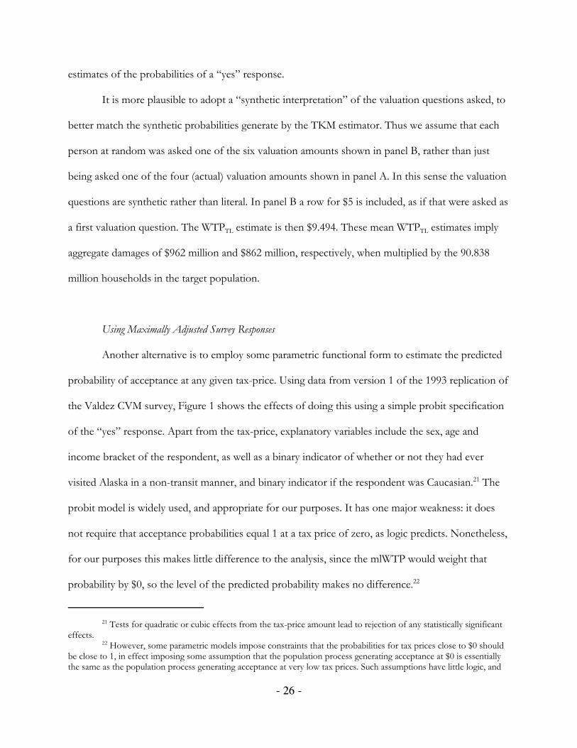
The solid dark line in the middle of the display in Figure 1 shows the average probability of

acceptance predicted by the model at each tax price. This is an average taken over the sample of 260

individual respondent predictions, assuming that the probit model is correct. The shaded area in the

middle show the 90% confidence interval, again over the sample of 260 predictions. Finally, the lines

on the outside show the smallest and largest individual predictions at each tax price.

It is important to appreciate that these predictions assume no error in the estimated model.

That is, this prediction takes the point estimates from the probit model and predicts a probability of

acceptance for each individual by applying the appropriate tax price and the characteristics of the

individual. It assumes that there is no sampling error in the estimates of the coefficients of the

model, when in fact there is an error. These predictions therefore convey a greater sense of

confidence in responses than would be obtained if one allowed for the uncertainty in the sample

estimates of these coefficients. This difference would show up in the confidence intervals and

extreme values in Figure 1, rather than the mean prediction.

From Figure 1, and recognizing that these predictions significantly understate the uncertainty

about the probabilities of acceptance, we see that the 50% acceptance probability point is within a

90% confidence interval for all tax prices up to $100, and the average is well below 50% for all

higher tax prices. These findings pose serious problems if one views the responses as the basis for

predicting the latent population process, since one could then argue23 that there is no statistically

significant basis for any positive damages amount!

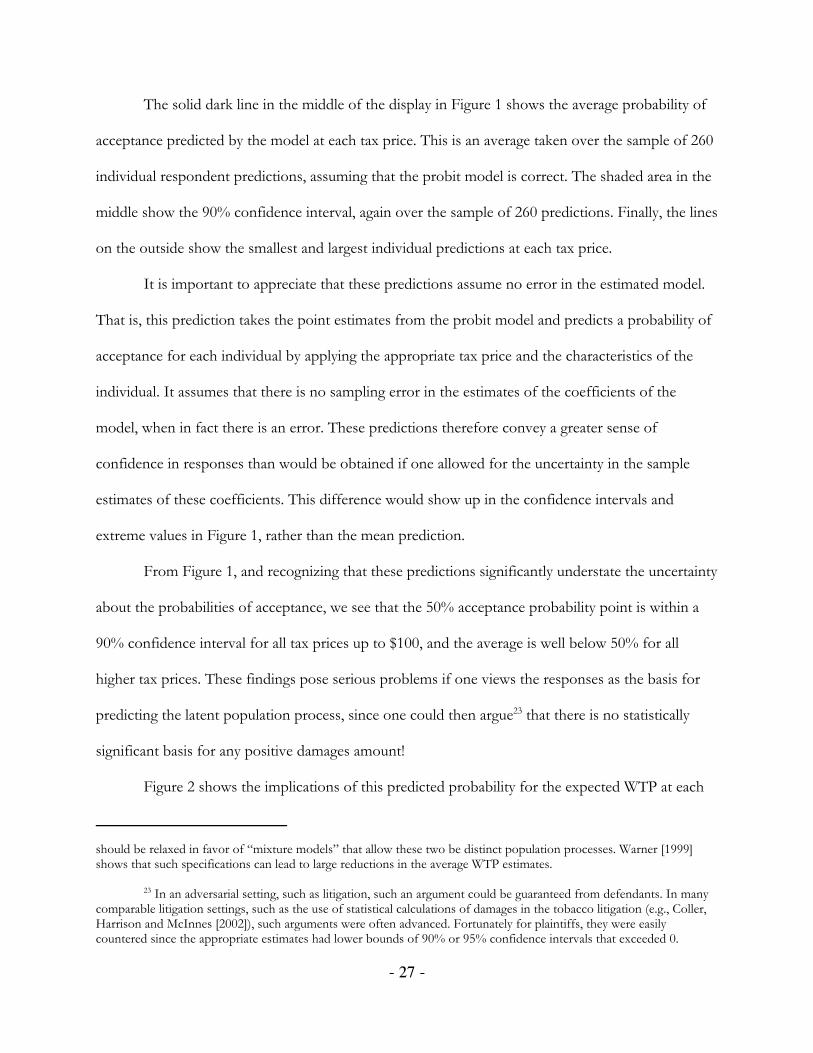
Figure 2 shows the implications of this predicted probability for the expected WTP at each

- 28 -

tax price. This line shows the expected payment if the given tax price was used for a subject drawn

at random from the population generating the responses embodied in the estimated probit model.

The vertical lines show the actual tax prices used. At tax prices of $10, $30, $60 and $120, each being

used with probability ¼ and with average probabilities of acceptance from Figure 1 of 0.61, 0.57,

0.49 and 0.35, respectively, the expected WTP at each tax price is $1.536 (=$10 × ¼ × 0.6145),

$4.254, $7.408 and $10.506. Thus the total mlWTP for the typical household is $23.705, for an

implied damages estimate of $2.153 billion.

Using the complete set of synthetic tax prices in Figure 2, which numerically amount to 501

tax prices between $0 and $500 in increments of $1, the mlWTP for the typical household is $15.301

for an implied damages estimate of $1.390 billion. Thus, conditional on the use of a common

parametric model to estimate the probabilities of acceptance, there is a difference in damages of

$763 million (= $2.153 billion - $1.390 billion) just by changing from the literal to the latent

interpretation of the CVM survey process.

A range between $0 and $500 seems reasonable since $500 is more or less where the

probability of acceptance drops to 0. But this is another issue of interpretation that has to be

resolved. If one employs an extremely wide interval damages can be made arbitrarily lower. For

example, assume the tax prices were $0, $500, $1000 and $2000. Each would have an expected WTP

of $0, so total damages would be zero. Taking the 1001 tax prices between $0 and $1001 in

increments of $1, to take a less contrived example, lowers aggregate damages from $1.390 billion to

just $696 million.

C. Scenario Ambiguity

One of the first “cultural” differences that strikes an experimental economist dipping his

toes into the sea of contingent valuation studies is how careful those studies are in their choice of

- 29 -

language on some matters and how appallingly vague they are on other matters. The best CVM

studies spend a lot time, and money, on “focus groups” in which they tinker with minute details of

the scenario and the granular resolution of pictures used in displays. But they often leave the most

basic of the “rules of the game” for the subject unclear.

For example, consider the words used to describe the scenario in the Valdez study. Forget

the simple majority-rule referendum interpretation used by the researchers, and focus on the words

actually presented to the subjects. The relevant passages concerning the provision rule are quite

vague on that rule.

How might the subjects be interpreting specific passages? Consider one hypothetical subject.

He is first told, “In order to present damages to the area’s natural environment from another spill, a

special safety program has been proposed. We are conducting this survey to find out whether this

special program is worth anything to your household.” (p.52). Are the proposers of this program

going to provide it no matter what I say, and then come for a contribution afterwards? In this case I

should free-ride, even if I value the good. Or are they actually going to use our responses to decide

on the program? If so, am I that Mystical Measure-Zero Median voter whose response might

“pivot” the whole project into implementation? In this case I should tell the truth.

Actually, the subject just needs to attach some positive subjective probability to the chance

of being the decisive voter. As that probability declines, so does the (hypothetical) incentive to tell

the truth. So, to paraphrase Dirty Harry the interviewer, “do you feel like a specific order statistic

today, punk?” Tough question, and presumably one that the subject has guessed at an answer to. I

am just adding additional layers of guesswork to the main story, to make clear the extent of the

potential ambiguity involved.

Returning to the script, the subjects are later told, “If the program was approved, here is

how it would be paid for.” But who will decide if it is to be approved? Me, or is that out of my

24 Each household was given a “price” which suggested that others may pay a different “price.” This isstandard in such referendum formats, and could be due to the vote being on some fixed formula that taxes thehousehold according to assessed wealth. Although the survey does not clarify this for the subjects, it would be an easymatter to do so.

- 30 -

hands as a respondent? As noted above, the answer matters for my rational response. The subjects

were asked if they had any questions about how the program would be paid for (p. 55), and had any

confusions clarified then. But this is no substitute for the control of being explicit and clear in the

prepared part of the survey instrument.

Later in the survey the subjects are told, “Because everyone would bear part of the cost, we

are using this survey to ask people how they would vote if they had the chance to vote on the

program.” (p.55). OK, this suggests that the provision rule would be just like those local public

school bond issues I always vote on, so the program will (hypothetically) go ahead if more than 50%

of those that vote say “yes” at the price they are asking me to pay.24 But I am bothered by that

phrase “if they had the chance to vote”: does this mean that they are not actually going to ask me to

vote and decide if the program goes ahead, but are just floating the idea to see if I would be willing

to pay something for it after they go ahead with the program? Again, the basic issue of the provision

rule is left unclear. The final statement of relevance does nothing to resolve this possible confusion:

“If the program cost your household a total of $(amount) would you vote for the program or against

it?” (p.56).

Is this just “semantics”? Yes, but it is not “just semantics.” Semantics are relevant if we

define it as the study of “what words mean and how these meanings combine in sentences to form

sentence meanings” (Allen [1995; p.10]). Semantics, along with syntax and context, are critical

determinants of any claim that a sentence in a CVM instrument can be unambiguously interpreted.

The fact that a unique set of words can have multiple, valid interpretations is well-known in general

to CVM researchers. Nonetheless, it appears to have also been well-forgotten in this instance, since

25 Statistical approaches to the linguistic issue of how people resolve ambiguous sentences in natural languagesare becoming quite standard. See, for example, Allen [1995; Ch.7, 10] and Schütze [1997; Ch.2], and the references citedthere. Non-statistical approaches, using axioms of conversation to dis-ambiguate sentences, are proposed in another lineof linguistic research by Grice [1989] and Clark [1992].

- 31 -

the subject simply cannot know the rules of the voting game he is being asked to play.

More seriously, we cannot claim as outside observers of his survey response that we know

what the subject is guessing at.25 We can, of course, guess at what the subject is guessing at. This is

what Carson et al. [1992] do when they choose to interpret the responses in one way rather than

another, but this is still just a dressed-up guess. Moreover, it is a serious one for the claim that

subjects have an incentive to free ride, quite aside from the hypothetical bias problem.

The general point is that one can avoid these problems with more explicit language about the

exact conditions under which the program would be implemented and payments elicited. I fear that

CVM researchers would shy away from such language since it would likely expose to the subject the

truth about the hypothetical nature of the survey instrument. The illusory attraction of the frying pan

again.

3. Advisory Survey Referenda

Survey referenda are used to evaluate social policy, particularly the valuation of

environmental resources. How should the responses to these referenda be interpreted? One view is

that they represent a social microcosm of how the population would vote, and that they should be

taken literally. The basic idea is that one is sampling a population voting process, and that process is

a valid social choice mechanism whose results should be respected. Thus the outcome of the vote is

all that matters, even if a representative sample chose not to vote. Another view is that the language

of the survey uses the frame of a referendum vote simply as a social metaphor, and that the

responses should be used to infer the underlying valuation. Thus the outcome of the vote, per se, has

26 Carson et al. [1997] compare the original Exxon Valdez survey referendum and the 1993 replication, findingno statistical difference between the two. The data from the original referendum are not available for public evaluation. Carson et al. [1994; Table 5-5, p.95] report that the raw percentage vote for the proposal in the original referendumsurvey was 68%, 52%, 50% and 36%, respectively, at tax-prices of $10, $30, $60 and $120. This compares with rawresponses of 68%, 56%, 49% and 33% in the 1993 replication.

- 32 -

no standing other than as a vehicle for eliciting information about how individuals would vote and

allowing statistical inferences about the “latent” population preferences.

Each approach has something to commend it, but the two interpretations can lead to

radically different inferences. These differences are particularly striking when respondents have a

choice as to whether or not to vote. If one is taking the survey referenda literally as a social choice,

then a failure to chose to vote is a valid response and should be counted as such. If one is taking the

survey as just a way of presenting the issue to respondents in a way that they can understand, there is

more leeway to use the responses to try to estimate the “latent” valuation underlying the observed

responses. In this case, one is free to infer some positive valuation for non-voters.

These issues can be made concrete by considering the use of survey referenda to place a

value on compensatory damages caused by the Exxon Valdez oil spill. We do so below, and then

review the way in which survey referenda are presented to respondents, as a guide to how their

responses are solicited.

A. The Exxon Valdez Replication

In 1993 a replication and extension of the ExxonValdez oil spill survey was conducted. The

replication was close, in the sense that essentially the same survey instrument was used from the

original study and the same in-person survey method used.26 Moreover, three treatments were added

that make the 1993 replication particularly interesting. One treatment was the use of a “ballot box”

in which the respondent could privately deposit their response, and did not have to reveal it to the

interviewer. Another treatment was the addition of a “no vote” option, such that respondents could

27 In the end, sample sizes for versions 1 through 4 were 300, 271, 322 and 289, or 25.4%, 22.9%, 27.2% and24.5%, respectively. Samples were drawn from 12 primary sampling units across the country.

28 One could use a simple probit estimator, in which the tax-price was an independent variable and the “for”

- 33 -

explicitly say whether they were “for,” “against,” “not sure” or “would not vote.” And a third

treatment was a cross of the last two: the “no vote” option was implemented with a ballot box. The

overall sample was 1,182, with roughly 25% allocated at random to each version.27 Within each

version, each subject was asked how they would vote if the cost to their household was a particular

amount, chosen at random from $10, $30, $60 or $120. In the surveys that did not use the ballot

box, respondents were asked a follow-up question based on their initial responses; we ignore these

follow-up responses, since they were not common over all versions and have some problems of

interpretation. Results from the 1993 replication were published in Carson et al. [1998] and Krosnick

et al. [2002].

Figure 3 displays the raw responses in each of the four versions. To simplify, the light grey

lines with a circle marker indicate responses “for” the proposed policy to avoid another oil spill over

the next 10 years, and the black lines with square markers indicate responses “against” the policy.

Dark grey lines with diamond markers, as appropriate, indicate “no vote” responses when asked for.

These responses have not been adjusted for any population weights, or complex survey sample

design features; nothing of consequence here is affected by those corrections.

The top left panel of Figure 3 shows that respondents tend to favor the policy on balance

when the tax-price is lowest, and that this net vote for the policy diminishes as the tax-price

increases. These results would suggest that the largest tax-price that would just receive a majority

vote would be around $60. The exact determination of the point at which the “for” responses equal

50% would be determined by applying one or other statistical estimators to the raw responses.

Although there is some debate over the best estimators to apply, for now we will simply use the

piecewise linear estimates connecting the raw responses.28

responses the dependent variable. In this case the estimated tax-price can be solved from the estimated equation, whichcould control for individual characteristics in the sample to ensure comparability across versions. Using the probit modelintroduced in Section 2 for use with version #1, one can calculate damages for versions 1 through 4 of $1.390 billion,$2.587 billion, $1.641 billion and $3.659 billion, respectively. These calculations employ synthetic tax prices between $1and $500 in increments of $1.

- 34 -

The use of the anonymous ballot box, in the top right panel of Figure 3, reduces the positive

and negative responses at the lowest tax-price of $10, but otherwise has relatively little effect in

relation to the “original recipe” used in version #1. As a consequence there is much less net support

for the proposal at that $10 level, which might become an issue if one recognized sampling errors

around these responses. But the main effect of the ballot box is to dampen enthusiasm for

respondents that are for or against the proposal at the lowest tax-price, suggesting that those

responses may have been affected by the presence of an observer of the vote.

The raw responses with the explicit “no vote” option are shown in the bottom left panel of

Figure 3. Compared to version #1, above it, there is a very slight increase in the “for” responses at

$10, and a marked reduction in the “against” responses. The other large change is the reduction in

the “against” responses at the $120 tax-price. Although the fraction of “no vote” responses

increases slightly with the tax-price, from 9% at $10 to 11% at $120, it is relatively constant with

respect to tax-price. Taken together, these changes suggests that this treatment may be picking up

respondents that originally voted against the proposal because they reject one or more aspects of the

scenario presented in the survey referendum.

When the no-vote and ballot box treatments are crossed, in version #4 shown in the bottom

right panel of Figure 3, the fraction of “no vote” responses goes up to around 15% for the lowest

tax-prices and then 21% for the highest tax price. The direct “for” and “against” responses at the

lowest tax-price are akin to those observed for version #2, in which the ballot box was the sole

treatment. However, both are lower due to the fraction siphoned off into a “no vote” response. In

fact, the policy scenario barely survives a vote even at the lowest tax-price level of $10.

29 Actually, voter turnout is the main focus of party activists prior to elections, and can vary dramatically fromelection to election.

30 Again, recall the Florida recount in the 2000 Presidential elections in the United States.

- 35 -

Figure 4 shows what the responses would be if we simply condition on voter turnout. When

political elections are held, or real referenda voted on, nobody says very much about the “vote that

might have been” if everyone had turned out.29 Instead, what matters in law is simply the vote count

based on those that chose to vote. The results for version #1 and version #2 are identical to those

shown in Figure 3, of course, since they had no option not to vote. But the bottom panels in Figure

4 suggest that the policy has a much better chance of survival if the conditional vote is examined. All

that is happening is that the votes “for” or “against” are both re-normalized by the same amount, so

that the vote for the proposal equals or exceeds 50% for tax-prices up to $60. Again, it should be

noted that no standard errors are being placed around these responses, but the 2000 Presidential

elections in the United States remind us that none need be as a matter of law.

Figures 5 and 6 examine the change in voting patterns due to the provision of the “no vote”

option, and varying with three different assumptions on how to interpret those that chose that

option. In each case we show version #3 compared to version #1, and version #4 compared to

version #2, since that makes the pure effect of the no-vote treatment clear. The solid lines are the

original responses, from Figure 3, and the dotted overlaid line is the set of responses from the

treatment with the no-vote option and the specific interpretation assumed. We also treat those that

said that there were “not sure” as equivalent to not voting – they correspond to those that turn up to

vote, go into the voting booth, and cast an invalid vote.30

Figure 5 shows the effect of assuming that a “no vote” response means that the individual

would not have turned up for the election, and hence that the referenda would stand or fall on the

votes actually cast by those that did turn up. In effect, it overlays the top two panels of Figure 2 (the

solid lines) with the bottom two panels of Figure 2 (the dotted lines).

31 The issue of temporal stability arose from the report of the NOAA Panel contained in Arrow et al. [1994].The concern was that public outrage soon after an oil spill might lead to relatively high valuations of damages comparedto valuations conducted much later. Without further assumptions about the propriety of valuation differences, however,there is no reason for one to believe that valuations ought to be temporally stable, as Carson et al. [1997; p.159ff.] note.Moreover, there is little a priori reason to expect valuations elicited 22 months after the oil spill to be different fromvaluations elicited 39 months after. The real issue here is likely to involve comparisons much closer to the time of thespill, although even then there is nothing to say that such valuations should be the same as later valuations.

- 36 -

The conclusion is that interpreting a “no vote” response in this manner significantly

improves the chances of approval of this policy. The tax-price at which the proposal is supported at

the 50% level is either $120 or around $100, depending on the use of the ballot box.

Figure 6, on the other hand, paints a different outcome for the policy. In this case the “no

vote” responses are interpreted as voting “against” the proposal, and the proposal fails at much

lower tax-prices. In the absence of a ballot box the referendum proposal barely passes at the $30

level, and with the ballot box it barely survives at the $10 level.

These results indicate that for one of the most important survey referenda ever mounted in

the field of environmental valuation, the inferences are very sensitive to how one interprets

responses. In the next section we review how previous studies have interpreted these responses.

B. Advisory Referenda in the Eyes of Researchers

Carson et al. [1997] consider version #1 only, and adopt (p.156) an agnostic stance with

respect to the “unsure” responses. They show the effects of interpreting them as “against,” as a

separate category, and as being irrelevant (in the sense of being deleted and allowing the existing

votes to be re-normalized). In context, their approach is appropriate, since they are only testing the

temporal stability of the responses from 1991 to 1993.31

Carson et al. [1998] consider version #1 and version #3 only, and adopt (p.336) the

interpretation of “no vote” responses employed in our Figure 6. Their comparison is actually a

hybrid of ones displayed here, so it is useful to visualize it explicitly. Figure 7 does so, also including

- 37 -

version #4 for good measure. The “for” responses are the raw ones shown in Figure 1, so they are

drawn with a solid line to indicate the raw response. The “against” responses are the constructed

responses based on the raw responses as well as the assumption that “no vote” and “unsure” are the

same as an “against” vote. Carson et al. [1998] conclude that the two left-hand panels in Figure 7 are

not statistically different. Since they look different to the naked eye, it is useful to go through the

statistical tests they use to draw their conclusion.

The first test is a simple contingency table test of independence, where one treatment is the

“for” or “against” response and the other treatment is the provision of a “no vote” option or not.

These undertake these tests for each tax-price. Thus, for the $10 tax-price for example, the 68% and

32% responses in the left panel (which are 59 individuals and 28 individuals) are compared to the

73% and 27% responses in the right panel (or 60 individuals and 22 individuals), using standard

tests. The χ2 statistic is 0.58 in this case, with a p-value of 0.45, so one cannot reject the null that

these treatments are independent. Similarly for the other tax-prices. The problem is that these tests

have extremely low power at these sample sizes. Using a p-value of 5% for a two-tailed test, one

would need samples of over 1500 per cell in order to reject the above null hypothesis with a power

of 0.90 or greater. Alternatively, with the actual samples of only 87 and 82, the power for tests of

this null hypothesis is only 0.086.

Figure 8 shows how bleak things are for any interesting hypothesis test using non-parametric

tests such as the one just refereed to. The null hypothesis in Figure 8 is that the “for” responses are

50% of the votes. The alternative hypotheses are that there is a 5, 10 or 15 percentage point

difference, to consider the range of practical interest here. The ability to detect a 5 percentage point

difference is very low indeed at samples of around 75, as indicated by the vertical line. Only when

samples get well above 1,000 can one begin to believe that these tests are detecting such differences

with any acceptable power. Of course, larger differences can be detected with greater power for the

32 Uncertainty in valuation does not imply that the valuation is always uninformative. Bohm [1984], in particular,stressed the use of multiple measuring instruments that might bound any (strategic) bias to misrepresent value. If all ofthose methods yield values that completely exceed or completely fall below the cost of a policy, crisp cost-benefitinferences can still be made.

- 38 -

same sample sizes, but even 15 percentage point differences will be detected with low power for

samples sizes around 75.

One implication is that, since the sample sizes cannot be increased, we must be prepared to

make some parametric assumptions about responses in order to detect differences due to these

treatments. This is what Carson et al. [1998] do, by considering parametric statistical models of

responses.

Returning to Figure 7, consider however the effect of moving from version #1 to version

#4: the referendum fails, or comes close to failing, at the lowest tax price of $10. It definitely fails at

any higher tax price. No statistical tests are needed in this case to see that the interpretation of the

CVM, plus the use of different versions, makes a huge difference to the implied damages.32

C. Advisory Referenda in the Field

Many field surveys are designed to avoid the problem of hypothetical bias, by presenting the

referenda as “advisory.” Great care is often taken in the selection of motivational words in cover

letters, opening survey questions, and key valuation questions, to encourage the subject to take the

survey seriously in the sense that their response will “count.” It is useful to examine some

prominent examples of this pattern, to identify the way that they are couched to subjects.

Consider the generic cover letter advocated by Dillman [1978; pp.165ff.] for use in mail

surveys. The first paragraph is intended to convey something about the social usefulness of the

study: that there is some policy issue which the study is attempting to inform. The second paragraph

is intended to convince the recipient of their importance to the study. The idea here is to explain

33 Cummings, Harrison and Osborne [1995], Cummings and Taylor [1999] and Harrison [2006] demonstratehow one could evaluate such “cheap talk” in a controlled experimental manner.

- 39 -

that their name has been selected as one of a small sample, and that for the sample to be

representative they need to respond. The goal is clearly to put some polite pressure on the subject to

make sure that their socio-economic characteristic set is represented.

The third paragraph ensures confidentiality, so that the subject can ignore any possible

repercussion from responding one way or the other in a “politically incorrect” manner. Although

seemingly mundane, this assurance can be important when the researcher interprets the subject as

responding to the question at hand rather than uncontrolled perceptions of repercussions. It also

serves to mimic the anonymity of the ballot box.

The fourth paragraph builds on the preceding three to drive home the usefulness of the

survey response itself, and the possibility that it will influence behavior:

The fourth paragraph of our cover letter reemphasizes the basic justification for the study -- its socialusefulness. A somewhat different approach is taken here, however, in that the intent of the researcher tocarry through on any promises that are made, often the weakest link in making study results useful, isemphasized. In {an example cover letter in the text} the promise (later carried out) was made to provideresults to government officials, consistent with the lead paragraph, which included a reference to billsbeing considered in the State Legislature and Congress. Our basic concern here is to make the promise ofaction consistent with the original social utility appeal. In surveys of particular communities, a promise isoften made to provide results to the local media and city officials. (Dillman [1978; p.171])

From our perspective, the clear intent and effect of these admonitions is to attempt to convince the

subject that their response will have some probabilistic bearing on actual outcomes. We do not need

to enter into any debate on whether this intent is realized.33

This generic approach has been used, for example, in the CVM study of the Nestucca oil spill

by Rowe, Schulze, Shaw, Schenk and Chestnut [1991]. Their cover letter contained the following

sentences in the opening and penultimate paragraphs:

Government and industry officials throughout the Pacific Northwest are evaluating programs to preventoil spills in this area. Before making decisions that may cost you money, these officials want your input. [...]The results of this study will be made available to representatives of state, provincial and federalgovernments, and industry in the Pacific Northwest. (emphasis added).

34 The cover letter was dated August 28, 1990.

- 40 -

In the key valuation question, subjects are motivated by the following words:Your answers to the next questions are very important. We do not yet know how much it will cost toprevent oil spills. However, to make decisions about new oil spill prevention programs that could cost youmoney, government and industry representatives want to learn how much it is worth to people like you toavoid more spills.

These words reinforce the basic message of the cover letter: there is some probability, however

small, that the response of the subject will have an actual impact.

More direct connections to policy impact occur when the survey is openly undertaken for a

public agency charged with making the policy decision. For example, the Resource Assessment

Commission of Australia was charged with making a decision on an application to mine in public

lands, and used a survey to help it evaluate the issue. The cover letter, signed by the Chairperson of

the Commission under the letterhead of the Commission, spelled out the policy setting clearly:

The Resource Assessment Commission has been asked by the Prime Minister to conduct an inquiry intothe use of the resources of the Kakadu Conservation Zone in the Northern Territory and to report to himon this issue by the end of April 1991.34 [...] You have been selected randomly to participate in a nationalsurvey related to this inquiry. The survey will be asking the views of 2500 people across Australia. It isimportant that your views are recorded so that all groups of Australians are included in the survey. (Imber,Stevenson and Wilks [1991; p.102])

Although no promise of a direct policy impact is made, the survey responses are obviously valued in

this instance by the agency charged with directly and publically advising the relevant politicians on

the matter.

There are some instances in which the agency undertaking the study is deliberately kept

secret to the respondent. For example, this strategy was adopted by Carson et al. [1992] in the Exxon

Valdez oil spill survey. They in fact asked subjects near the end of the survey who they thought had

sponsored the study, and only 11% responded correctly (p.91). However, 29% thought that Exxon

had sponsored the study. Although no explicit connection was made to suggest who would be using

the results, it is therefore reasonable to presume that at least 40% of the subjects expected the

responses to go directly to one or other of the litigants in this well-known case. Of course, that does

not ensure that the responses will have a direct impact, since there may have been some (rational)

35 In other words, there are circumstances when one wants to include such uncertainty in the scenario. Considera setting in which the tax instrument could be a general sales tax or a specific excise tax, and the decision between thetwo is to be made later in the political process. Asking subjects their willingness to contribute conditional on one orother instrument would misrepresent the true situation, which is that the respondent is being asked to state hiswillingness to contribute to an ill-defined lottery.

- 41 -

expectation that the case would settle without the survey results being entered as evidence.

4. Overall Assessment

The general problem with the Exxon Valdez study is that it suffers from blind spots. There

are three types of blind spots involved: simple grammatical disambiguation, the appropriate social

welfare function underlying the damages calculation, and the relative role of data and assumptions

when drawing inferences about the responses.

On some matters of phraseology it is apparent that extraordinary care and billable consultant

hours were applied. And yet there are some fundamental matters that seem to have been developed

with little or no thought. The exposition of the financial contribution part of the basic scenario is

simply vague. Perhaps this was deliberate, to reflect some underlying uncertainty in the scenario,35

but more likely it was just a corollary of having a hypothetical valuation question at the heart of the

instrument. If the respondents know that their monetary contributions are not real, then they have

no incentive to take the “rules of the game” seriously and, presumably, the investigator might be

relieved of the responsibility of stating them coherently. A lack of control of responses, and

corresponding ambiguity for valuation inferences, is the only consequence of such design choices.

The second blind spot is the issue of how to calculate descriptive measures of the responses.

This cannot be resolved without knowing how the responses are to be used, which relates to the

implicit choice of a social welfare function. No justifiable case exists for the use of the median when

one is trying to ascertain the aggregate amount of money needed to compensate a group of

individuals, particularly when the population process is known a priori to be heavily skewed. If one

member of society requires $100 to be compensated for the environmental injury, and the other 99

- 42 -

need nothing, we still need to raise $100 from defendants to make all 100 members of society whole.

If the compensation is supposed to be “for society as a whole” then it is not obvious that one wants

to use a simple majority rule elicitation device for determining the amount. The reason is essentially

the same as in the previous example of 100 people: there could be a “tyranny of the majority” that

might require nothing and vote accordingly, leaving the one member of society to incur a loss of

$100.

Of course, those 99 might also vote to ensure compensation of the 100th person in society, if

they had some sense that his damages were real. But then we have to clearly state the purpose of the

advisory survey referenda, which is the final blind spot. Is the referenda to be viewed as a process

that just helps the respondent frame the issue, and that allows the researcher to take the responses

and use them to infer some latent population mean? Or is the referenda to be viewed as a literal or

legal voting process, where one has to live with the voters that turnout and record proper votes?

Until we have some basis for resolving these matters of interpretation, the estimation of damages for

the Exxon Valdez oil spill remain a matter of speculation. Given the significance of this case, this is

unfortunate.

References

Allen, James, Natural Language Understanding (Redwood City, CA: Benjamin/Cummings, SecondEdition, 1995).

Arrow, Kenneth; Solow, Robert; Portney, Paul; Leamer, Edward E.; Radner, Roy; and Schuman,Howard, “Report of the NOAA Panel on Contingent Valuation,” Federal Register, 58(10),January 15, 1993, 4602-4614.

Bishop, Richard C., and Heberlein, Thomas A., “Measuring Values of Extramarket Goods: AreIndirect Measures Biased?” American Journal of Agricultural Economics, 61, December 1979, 926-930.

Blackburn, McKinley; Harrison, Glenn W., and Rutström, E. Elisabet, “Statistical Bias Functionsand Informative Hypothetical Surveys”, American Journal of Agricultural Economics, 76(5),December 1994, 1084-1088.

Bohm, Peter, “Revealing Demand for An Actual Public Good,” Journal of Public Economics, 24, 1984,135-151.

Carson, Richard T., “Kakadu Conservation Zone”, in K.M. Ward and J.W. Duffield (eds.), NaturalResource Damages: Law and Economics (New York: Wiley, 1992).

Carson, Richard T., “Contingent Valuation: Theoretical Advances and Empirical Tests Since theNOAA Panel,” American Journal of Agricultural Economics, 79(5), December 1997, 1501-1507.

Carson, Richard T.; Conaway, Michael B.; Hanemann, W. Michael; Kopp, Raymond J.; Krosnick,Jon A.; Martin, Kerry M.; McCubbin, Donald R.; Mitchell, Robert C.; and Presser, Stanley,The Value of Preventing Oil Spill Injuries to Natural Resources Along California’s Central Coast(Washington, DC: National Oceanic and Atmospheric Administration, March 31 1996, twovolumes).

Carson, Richard T.; Flores, Nicholas E., and Meade, Norman F., “Contingent Valuation:Controversies and Evidence,” Environmental and Resource Economics, 19, 2001, 173-210.

Carson, Richard T.; Hanemann, W. Michael; Kopp, Raymond J.; Krosnick, Jon A.; Mitchell, RobertC.; Presser, Stanley; Ruud, Paul A.; and Smith, V. Kerry, Prospective Interim Lost Use Value Dueto DDT and PCB Contamination in the Southern California Bight (Washington, DC: NationalOceanic and Atmospheric Administration, September 1994, two volumes).

Carson, Richard T; Hanemann, W. Michael; Kopp, Raymond J.; Krosnick, Jon A.; Mitchell, RobertC.; Presser, Stanley; Ruud, Paul A., Smith, V. Kerry, “Temporal Reliability of Estimates fromContingent Valuation,” Land Economics, 73(2), May 1997, 151-163.

Carson, Richard T; Hanemann, W. Michael; Krosnick, Jon A.; Mitchell, Robert C.; Presser, Stanley;Ruud, Paul A., Smith, V. Kerry, “Referendum Design and Contingent Valuation: TheNOAA Panel’s No-Vote Recommendation,” Review of Economics and Statistics, 80(2), May1998, 335-338; reprinted with typographical corrections in Review of Economics and Statistics,80(3), August 1998.

Carson, Richard T.; Mitchell, Robert C.; Hanemann, W. Michael; Kopp, Raymond J.; Presser,Stanley; and Ruud, Paul A., A Contingent Valuation Study of Lost Passive Use Values ResultingFrom the Exxon Valdez Oil Spill (Anchorage: Attorney General of the State of Alaska,November 1992).

Carson, Richard T.; Mitchell, Robert C.; Hanemann, W. Michael; Kopp, Raymond J.; Presser,Stanley; and Ruud, Paul A., “Contingent Valuation and Lost Passive Use: Damages from theExxon Valdez”, Environmental and Resource Economics, 25, 2003, 257-286.

Carson, Richard T.; Wilks, Leanne; and Imber, David, “Valuing the Preservation of Australia'sKakadu Conservation Zone,” Oxford Economic Papers, 46, 1994, 727-749.

Clark, Herbert H., Arenas of Language Use (Chicago: University of Chicago Press, 1992).

Coller, Maribeth; Harrison, Glenn W., and McInnes, Melayne Morgan, “Evaluating the TobaccoSettlement: Are the Damages Awards Too Much or Not Enough?” American Journal of PublicHealth, 92(6): 2002, 984-989.

Cummings, Ronald G.; Elliott, Steven; Harrison, Glenn W., and Murphy, James, “Are HypotheticalReferenda Incentive Compatible?” Journal of Political Economy, 105(3), June 1997, 609-621.

Cummings, Ronald G., and Harrison, Glenn W., “Was the Ohio Court Well Informed in TheirAssessment of the Accuracy of the Contingent Valuation Method?” Natural Resources Journal,34(1), Winter 1994, 1-36.

Cummings, Ronald G.; Harrison, Glenn W., and Osborne, Laura L., “Are Realistic Referenda Real?”Economics Working Paper B-95-06, Department of Economics, University of South Carolina,1995; available at http://www.bus.ucf.edu/gharrison/wp/.

Cummings, Ronald G.; Harrison, Glenn W., and Rutström, E. Elisabet, “Homegrown Values andHypothetical Surveys: Is the Dichotomous Choice Approach Incentive Compatible?”American Economic Review, 85(1), March 1995, 260-266.

Cummings, Ronald G. and Taylor, Laura O., “Unbiased Value Estimates for Environmental Goods:A Cheap Talk Design for the Contingent Valuation Method,” American Economic Review,89(3), June 1999, 649-665.

Dillman, Don A., Mail and Telephone Surveys: The Total Design Method, Wiley (New York: 1978).

Grice, Paul, Studies in the Way of Words (Cambridge, MA: Harvard University Press, 1989).

Hanemann, W. Michael, “Welfare Evaluations in Contingent Valuation Experiments with DiscreteResponse Data: Reply,” American Journal of Agricultural Economics, 71, November 1989, 1057-1061.

Hanemann, W. Michael, “Review”, in D. Imber, G. Stevenson, and L. Wilks, A Contingent ValuationSurvey of the Kakadu Conservation Zone (Canberra: Australian Government Publishing Servicefor the Resource Assessment Commission, February 1991).

Harrison, Glenn W., “Experimental Evidence On Alternative Environmental Valuation Methods,”Environmental and Resource Economics, 2006, forthcoming.

Harrison, Glenn W; Jensen, Jesper; Lau, Morten Igel, and Rutherford, Thomas F., “Policy ReformWithout Tears,” A. Fossati and W. Weigard (eds.), Policy Evaluation With Computable GeneralEquilibrium Models (New York: Routledge, 2001).

Harrison, Glenn W., and Kriström, Bengt, “On the Interpretation of Responses to ContingentValuation Surveys”, in P.O. Johansson, B. Kriström and K.G. Mäler (eds.), Current Issues inEnvironmental Economics (Manchester: Manchester University Press, 1996).

Harrison, Glenn W.; Rutherford, Thomas F., and Tarr, David G., “Trade Liberalization, Poverty andEfficient Equity,” Journal of Development Economics, 71, June 2003, 97-128.

Hausman, Jerry A. (Ed.), Contingent Valuation: A Critical Assessment (Amsterdam: North-Holland,1993).

Imber, David; Stevenson, Gay; and Wilks, Leanne, A Contingent Valuation Survey of the KakaduConservation Zone (Canberra: Australian Government Publishing Service for the ResourceAssessment Commission, 1991).

Johansson, Per-Olov; Kriström, Bengt; and Mäler, Karl-Göran, “Welfare Evaluations in ContingentValuation Experiments with Discrete Response Data: Comment,” American Journal ofAgricultural Economics, 71, November 1989, 1054-1056.

Kaplan, E.L., and Meier, P., “Nonparametric Estimation from Incomplete Observations,” Journal ofthe American Statistical Association, 53, June 1958, 457-481.

Kriström, Bengt, “A Non-Parametric Approach to the Estimation of Welfare Measures in DiscreteResponse Valuation Studies,” Land Economics, 66, May 1990, 135-139.

Krosnick, Jon A.; Holbrook, Allyson L.; Berent, Matthew K.; Carson, Richard T.; Hanemann, W.Michael; Kopp, Raymond J.; Mitchell, Robert C.; Presser, Stanley; Ruud, Paul A. Ruud;Smith, V. Kerry; Moody, Wendy R.; Green, Melanie C., and Conaway, Michael, “The Impactof ‘No Opinion’ Response Options on Data Quality: Non-Attitude Reduction or anInvitation to Satisfice?” Public Opinion Quarterly, 66, 2002, 371-403.

Mead, Walter J., “Review and Analysis of Recent State-of-the-Art Contingent Valuation Studies”, inHausman, J. (ed.), Contingent Valuation: A Critical Appraisal (Amsterdam: North-Holland,1993).

National Oceanic and Atmospheric Administration, “Contingent Valuation Panel, Public Meeting,Wednesday, August 12, 1992,” Certified Official Transcript, 283 pp. plus attachments,Department of Commerce, Washington, DC., 1992.

National Oceanic and Atmospheric Administration, “Natural Resource Damage Assessments;Proposed Rules,” Federal Register, 59, no.5, January 7, 1994 (Part II).

Neill, Helen R.; Cummings, Ronald G.; Ganderton, Philip T.; Harrison, Glenn W., and McGuckin,

Thomas, “Hypothetical Surveys and Real Economic Commitments,” Land Economics, 70(2),May 1994, 145-154.

Rowe, Robert D.; Schulze, William D.; Shaw, W. Douglass; Schenk, David, and Chestnut, LauraineG., “Contingent Valuation of Natural Resource Damage Due to the Nestucca Oil Spill,”Final Report, RCG/Hagler, Bailly, Inc., Boulder, June 15, 1991.

Schütze, Hinrich, Ambiguity Resolution in Language Learning (Stanford: CLSI Publications, 1997).

Turnbull, Bruce W., “Nonparametric Estimation of a Survivorship Function with Doubly CensoredData,” Journal of the American Statistical Association, 69, March 1974, 169-173.

Werner, Megan, “Allowing for zeros in dichotomous-choice contingent-valuation models,” Journal ofBusiness & Economic Statistics, 17(4), 1999, 479-486.

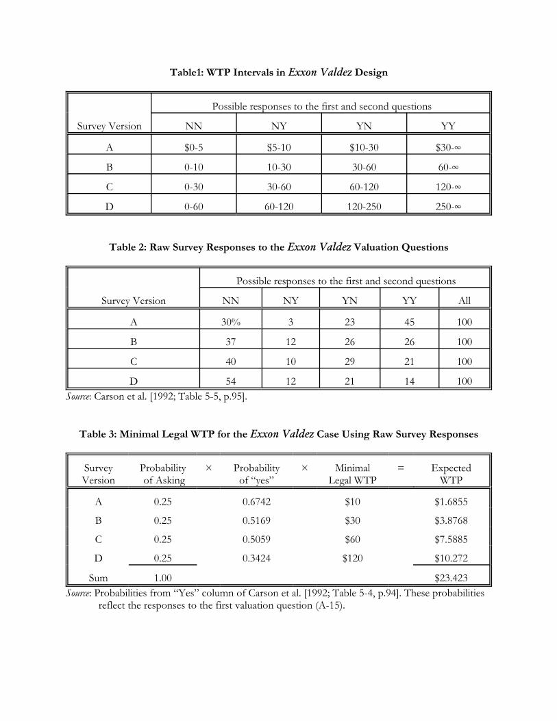
Table1: WTP Intervals in Exxon Valdez Design

Possible responses to the first and second questions

Survey Version NN NY YN YY

A $0-5 $5-10 $10-30 $30-4

B 0-10 10-30 30-60 60-4

C 0-30 30-60 60-120 120-4

D 0-60 60-120 120-250 250-4

Table 2: Raw Survey Responses to the Exxon Valdez Valuation Questions

Possible responses to the first and second questions

Survey Version NN NY YN YY All

A 30% 3 23 45 100

B 37 12 26 26 100

C 40 10 29 21 100

D 54 12 21 14 100Source: Carson et al. [1992; Table 5-5, p.95].

Table 3: Minimal Legal WTP for the Exxon Valdez Case Using Raw Survey Responses

SurveyVersion

Probability of Asking

× Probabilityof “yes”

× MinimalLegal WTP

= ExpectedWTP

A 0.25 0.6742 $10 $1.6855

B 0.25 0.5169 $30 $3.8768

C 0.25 0.5059 $60 $7.5885

D 0.25 0.3424 $120 $10.272

Sum 1.00 $23.423Source: Probabilities from “Yes” column of Carson et al. [1992; Table 5-4, p.94]. These probabilities

reflect the responses to the first valuation question (A-15).

Table 4: Minimal Legal WTP for the Exxon Valdez Case Using Estimated TKM Responses

SurveyVersion

Probability of Asking

× Probabilityof “yes”

× MinimalLegal WTP

= ExpectedWTP

A. Literal Interpretation of Valuation Questions

A 0.25 0.157 $10 $0.393

B 0.25 0.119 $30 $0.893

C 0.25 0.148 $60 $2.22

D 0.25 0.236 $120 $7.08

Sum 1.00 $10.585

B. Synthetic Interpretation of Valuation Questions

0.1667 0.036 $5 $0.030

0.1667 0.157 $10 $0.262

0.1667 0.119 $30 $0.595

0.1667 0.148 $60 $1.480

0.1667 0.125 $120 $2.501

0.1667 0.111 $250 $4.626

Sum 1 $9.494Source: Probabilities from “Change in Density” column of Carson et al. [1992; Table 5-6, p.97].

These probabilities are based on a statistical analysis of responses to all three valuationquestions (A-15, A-16 and A-17).

0

.25

.5

.75

1

Proba

bilit

y

0 50 100 150 200 250 300 350 400 450 500

Proposed Tax Price in Dollars

AssumingProbit Model and

No Prediction Error

Figure 1: Probability of Acceptanceof Exxon Valdez CVM Tax Price

0

.02

.04

.06

.08

Dolla

rs

0 50 100 150 200 250 300 350 400 450 500

Proposed Tax Price in Dollars

Figure 2: Expected Household WTPfrom Probit Model Predictions

0.00

0.25

0.50

0.75

0.00

0.25

0.50

0.75

10 30 60 120 10 30 60 120

1. Original Recipe 2. Ballot box

3. No vote option 4. No vote option & ballot box

Dollar amount asked to pay

Figure 3: Raw Responsesin 1993 Exxon Valdez CVM Survey

0.00

0.25

0.50

0.75

0.00

0.25

0.50

0.75

10 30 60 120 10 30 60 120

1. Original Recipe 2. Ballot box

3. No vote option 4. No vote option & ballot box

Dollar amount asked to pay

Figure 4:Responses Conditional On Voter Turnout

0.00

0.25

0.50

0.75

10 30 60 120 10 30 60 120

3. No vote option 4. No vote option & ballot box

Dollar amount asked to pay

Figure 5:Effect of Endogenous Voter Turnout

If 'No Vote' or 'Unsure' Responses Mean No Turnout

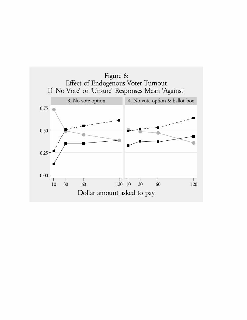
0.00

0.25

0.50

0.75

10 30 60 120 10 30 60 120

3. No vote option 4. No vote option & ballot box

Dollar amount asked to pay

Figure 6:Effect of Endogenous Voter Turnout

If 'No Vote' or 'Unsure' Responses Mean 'Against'

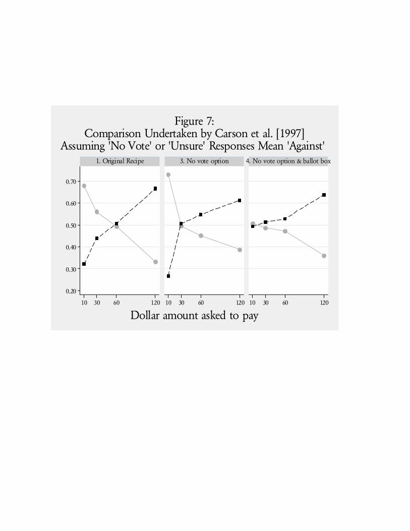
0.20

0.30

0.40

0.50

0.60

0.70

10 30 60 120 10 30 60 120 10 30 60 120

1. Original Recipe 3. No vote option 4. No vote option & ballot box

Dollar amount asked to pay

Figure 7:Comparison Undertaken by Carson et al. [1997]

Assuming 'No Vote' or 'Unsure' Responses Mean 'Against'

0.1.2.3.4.5.6.7.8.91

Power

0 200 400 600 800 1000Sample Sizes

5% difference10% difference15% difference

Power curves for test of null hypothesis of 50% 'yes' responsesFigure 8: Power Calculations