Embed Size (px)
Citation preview
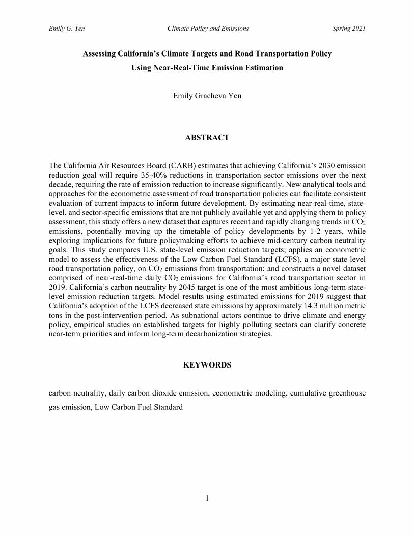
Emily G. Yen Climate Policy and Emissions Spring 2021
1
Assessing California’s Climate Targets and Road Transportation Policy
Using Near-Real-Time Emission Estimation
Emily Gracheva Yen
ABSTRACT
The California Air Resources Board (CARB) estimates that achieving California’s 2030 emission reduction goal will require 35-40% reductions in transportation sector emissions over the next decade, requiring the rate of emission reduction to increase significantly. New analytical tools and approaches for the econometric assessment of road transportation policies can facilitate consistent evaluation of current impacts to inform future development. By estimating near-real-time, state-level, and sector-specific emissions that are not publicly available yet and applying them to policy assessment, this study offers a new dataset that captures recent and rapidly changing trends in CO2 emissions, potentially moving up the timetable of policy developments by 1-2 years, while exploring implications for future policymaking efforts to achieve mid-century carbon neutrality goals. This study compares U.S. state-level emission reduction targets; applies an econometric model to assess the effectiveness of the Low Carbon Fuel Standard (LCFS), a major state-level road transportation policy, on CO2 emissions from transportation; and constructs a novel dataset comprised of near-real-time daily CO2 emissions for California’s road transportation sector in 2019. California’s carbon neutrality by 2045 target is one of the most ambitious long-term state-level emission reduction targets. Model results using estimated emissions for 2019 suggest that California’s adoption of the LCFS decreased state emissions by approximately 14.3 million metric tons in the post-intervention period. As subnational actors continue to drive climate and energy policy, empirical studies on established targets for highly polluting sectors can clarify concrete near-term priorities and inform long-term decarbonization strategies.
KEYWORDS
carbon neutrality, daily carbon dioxide emission, econometric modeling, cumulative greenhouse
gas emission, Low Carbon Fuel Standard
Emily G. Yen Climate Policy and Emissions Spring 2021
2
INTRODUCTION
The Intergovernmental Panel on Climate Change (IPCC) projects that meeting Paris
Agreement goals will require all countries to be carbon neutral, or have net zero CO2 emissions,
by mid-century, in conjunction with reductions in non-CO2 greenhouse gas (GHG) emissions. The
United Nations Secretary-General has called for this commitment from G20 countries since 2018
and asked for greater ambition in national climate plans before the 2021 UN Climate Change
Conference. The United States’ Paris Agreement goal to reduce emissions by 10-17% below 1990
levels by 2025, excluding land-use, land-use change and forestry (LULUCF), is not consistent
with the Paris Agreement goals of holding the increase in the global average temperature to well
below 2°C above pre-industrial levels and pursuing efforts to limit the temperature increase to
1.5°C above pre-industrial levels, as recommended by the IPCC (Masson-Delmotte et al. 2018).
The federal policies under the Trump Administration are projected to lead to only a 11-13%
reduction in emissions below 2005 levels by 2025, excluding LULUCF. Prior to January 2021, the
void left by the federal government during the Trump Administration resulted in subnational action
taking the lead in climate and energy policy (America’s Pledge 2020, Hsu et al. 2018). A growing
number of U.S. states have set mid-century carbon neutrality targets following California’s lead in
2018 and President Biden pledged a 2050 carbon neutrality target in 2021. California co-founded
the United States Climate Alliance (USCA) with New York and Washington States in an effort to
work towards the U.S. Nationally Determined Contribution in the absence of federal action (USCA
2020). With increased momentum on the international, national, and subnational levels to pursue
mid-century carbon neutrality targets and GHG emission reduction goals, empirical research on
climate policy impacts is necessary to aid future policy amendments. Studies such as E3’s
Pathways for Achieving Carbon Neutrality in California have broken down the specific measures
applied in carbon neutrality scenarios for various sectors. In-depth exploration of decarbonization
measures and policies by sector in the California context is appropriate because comprehensive
policy packages are often disaggregated into specific measures along sectoral lines. A highly
critical sector vital to the energy transition is transportation- especially road transportation, which
currently accounts for the largest source of emissions in California, outpacing the industrial,
agricultural, and residential sectors combined.

Emily G. Yen Climate Policy and Emissions Spring 2021
3
Subnational policymaking in the transportation sector is especially critical to meeting Paris
Agreement goals. Emissions from the global transportation sector account for almost one-quarter
of GHG emissions and approximately 72% of this amount is from road transportation (Axsen et
al. 2020). Transportation accounts for 41% of California’s overall emissions, due mostly to
passenger vehicles, and the share rises to nearly 55% when carbon emissions from producing
gasoline and diesel are included. State transportation emissions have continued to increase largely
due to increased driving miles, while emissions in nearly every other sector have declined in recent
years (CARB 2020). Transportation emissions are expected to grow further in scenarios produced
by the International Energy Agency (IEA), even if currently announced policies are implemented
(Creutzig et al. 2011). Assessing the effectiveness of current road transportation policies and
comparing emission reduction ambition is critical to identifying state policy gaps, or where greater
policy implementation and ambition is necessary to advance Paris goals (Creutzig et al. 2011).
California’s road transportation standards are pioneering- far more stringent than federal
standards- and state technologies and strategies have in many cases served as a model for other
states and jurisdictions around the world (Sperling and Eggert 2014). To better understand the
potential for road transportation policies to reduce global emissions, it is essential to assess
California’s policies in the context of wider subnational policy ambitions; analyze policy
effectiveness, taking into account the economic structure of jurisdictions; and utilize new emission
estimation data in policy analysis.
When assessing California’s policies in the road transportation sector, it is important to pay
particular attention to implementation gaps for meeting emission reduction targets. California’s
ambitious mid-term and long-term goals for reducing GHG emissions include a 40% reduction
below 1990 levels by 2030 and achieving carbon neutrality, or net zero GHG emissions, by 2045.
The California Air Resources Board (CARB) estimates that achieving the 2030 goal will require
35-40% reductions in transportation sector emissions over the next decade, requiring the rate of
emission reduction to increase significantly. Over the years, California has adopted a
comprehensive set of policies, regulations, and incentives to reduce GHG emissions in this sector,
focusing on vehicles, fuels, and mobility in the policy mix (Kern and Howlett 2009). Policy mixes-
a common term referring to the presence of multiple policies implemented in the same region,
during the same time period, and relating to the same objective- have been studied extensively in
the literature (Axsen et al. 2020). While California drew many lessons from other regions and
Emily G. Yen Climate Policy and Emissions Spring 2021
4
jurisdictions in designing climate policies, few other policy mixes are as comprehensive and
ambitious (Sperling and Eggert 2014). By identifying the differences between other state policies
and California’s approach, researchers can better assess the level of ambition and potential room
for improvement for this sector. California’s Low Carbon Fuel Standard (LCFS) is a prominent
climate policy, aiming to limit the state’s CO2 footprint of on-road vehicles (Creutzig et al. 2011,
Sperling and Eggert 2018, USCA 2020). This regulation can play a leading role in policy mixes in
many regions due to its potential effectiveness and political acceptability (Axsen et al. 2020).
However, the impact of the LCFS on emissions has not been extensively studied; furthermore, the
application of near-real-time emissions in policy analysis for this sector has not been greatly
utilized. This data is critical because it allows researchers to identify structural changes due to
recent developments, helping subnational governments to adjust ineffective policies and reinforce
necessary ones more quickly (Liu et al. 2020a, Liu et al. 2020b). By using recent data and
examining the ambition and effectiveness of current state policies in reducing emissions for this
sector, we can better predict the outcomes of future policies. There is no recent empirical work
that uses real-time daily CO2 emissions data coupled with econometric techniques to examine the
impact of U.S. state-level LCFS policies on CO2 emissions from the road transportation sector.
The question posed in this study is, how ambitious and effective are California’s major climate
targets and policy in the road transportation sector? Three sub-questions follow:
1. How ambitious are California’s climate targets compared to other states’ targets?
2. How effective are U.S. LCFS policies in reducing state-level CO2 emissions for the
transportation sector, using U.S. Energy Information Administration (EIA) transportation
emissions data?
3. Can state-level real-time daily CO2 emissions for road transportation be estimated to
examine LCFS effectiveness for this sector?
I highlighted and compared major state emission reduction targets in terms of timelines and levels
of commitment, with legislation and executive orders considered to be higher levels of
commitment, expecting California to have more ambitious mid-term or long-term emission
reduction targets and more binding commitments in the form of legislation and executive orders.
I examined LCFS policy impacts on CO2 emissions from the transportation sector using panel data
for U.S. states over the period 2000–2017, Stata 16 (StataCorp 2019), and economic regressions
clustered at the state level, expecting the LCFS to have been a highly effective policy that
Emily G. Yen Climate Policy and Emissions Spring 2021
5
decreased transportation sector emissions. I estimated state-level real-time daily CO2 emissions
for the road transportation sector and used this data to examine LCFS policy impacts on CO2
emissions, expecting consistent results.
BACKGROUND
State climate targets and policies
Twenty-seven states have pledged specific mid-term or long-term targets to reduce their
overall GHG or carbon emissions through legislation, executive orders, announcements, or
recommendations (USCA 2020). Nine states have gone further by enacting carbon neutral or net-
zero commitments via legislation or executive orders. Since California’s landmark Global
Warming Solutions Act of 2006 (AB 32) and the 2016 Senate Bill 32 were passed, California has
pioneered subnational climate action and continually extended and strengthened limits on GHG
emissions. The state grew its economy while decreasing carbon pollution and strengthening its
climate and energy policy portfolio. To understand the ambition and level of commitment of
California’s emission reduction policies, it is useful to consider the types and timelines of emission
targets across different states. Because state targets use different baseline years for emission
reduction, a common baseline year can be used to compare targets. Level of commitment can be
approached by categorizing policies into legislation, executive orders, announced plans, and
recommended goals. Binding legislation is more stringent because it generally provides tangible
incentives. Recommendations and announcements can be considered less stringent as they
generally do not provide tangible incentives. Executive orders have several caveats; future
governors can decide not to follow through with commitments by previous governors and
executive orders are rarely enforceable in court. In this study, legislation and executive orders are
considered to be more stringent commitments than announced plans and recommended goals.
While carbon neutrality, net-zero, and climate neutrality are often used interchangeably,
the IPCC provides a clear definition for each term. Carbon neutrality refers to a balance between
the CO2 emitted into the atmosphere and the CO2 removed from the atmosphere; net-zero emission
encompasses all GHG emissions and can refer to balancing emitted GHGs with removed GHGs
within a certain period of time; and climate (GHG) neutrality goes even further by considering all
Emily G. Yen Climate Policy and Emissions Spring 2021
6
human impacts that affect the climate, meaning that the targets are interpreted as implying net-
zero emissions for GHG (including LULUCF). The Paris Agreement defines carbon neutrality as
a balance between anthropogenic emissions by sources and removals by sinks of GHGs. The U.S.
federal government has no official definition of carbon neutrality and the net-zero emissions target
in President Biden’s Climate Plan does not specify whether it pertains to CO2 or all GHG gases.
The distinction between carbon neutrality and GHG neutrality is important because it can result in
significant differences in the estimated 2050 emissions level. This study does not seek to provide
a single definition of carbon neutrality, but considers the range of state targets. California defines
its carbon neutrality target as, “the point at which the removal of carbon pollution from the
atmosphere meets or exceeds emissions” (EO B-55-18). Hawaii, on the other hand, in its HB 2182
and HB 1986, sets the carbon neutrality goal of “sequestering more atmospheric carbon and
greenhouse gases than the State produces as quickly as practicable, but no later than 2045.”
Another example is Michigan’s goal, which aims to end net carbon emissions by 2050 “and to
maintain net negative greenhouse gas emissions thereafter.” The differences in wording illustrates
how carbon neutrality goals are not always defined the same way. Since in some cases, state
legislation has set carbon neutrality targets in terms of total GHG emissions rather than CO2
emissions, this study considers all state-level carbon neutrality, net-zero, and GHG neutrality target
values to be 100% GHG emission reduction goals.
Low Carbon Fuel Standard (LCFS)
LCFS policies are carbon intensity standards which primarily aim to reduce emissions from
transportation fuels without prescribing fuel type. An LCFS looks at the whole life cycle of the
fuel, applying standards to all stages of motor fuel production, and measures intensity rather than
absolute emissions. Regulated parties include all entities that either produce or import motor fuels
for consumption in the jurisdiction; regulated fuel providers are usually required to reduce average
fuel carbon intensity by some amount from a defined baseline year. By setting annual carbon
intensity benchmarks which reduce over time for gasoline, diesel, and their replacement fuels, the
LCFS provides policymakers another avenue to reduce transportation emissions and allows the
market to determine the fuel mix to be used to reach targets. LCFS programs generally allow for
Emily G. Yen Climate Policy and Emissions Spring 2021
7
trading and banking of emission credits to further enhance flexibility and support innovation
(C2ES 2019).
California was the first state to adopt the LCFS to reduce emissions from on-road light-
duty vehicles and transition away from liquid transportation fuels. In 2009, CARB approved the
LCFS regulation, a key AB 32 measure, to reduce the carbon intensity of transportation fuel used
in the state by at least 10% from 2010 levels by 2020 (Executive Order S-1-07). In 2018, CARB
approved amendments including strengthening the carbon intensity benchmarks through 2030,
with a target of 20% carbon intensity reduction from 2010 levels. As the LCFS is one of the first
attempts to bring the life-cycle CO2 emission concept into policy, it is not surprising that the life-
cycle accounting was challenged by certain stakeholders until the U.S. 9th Circuit Court ruled that
the LCFS would reduce CO2 emissions and that California should be encouraged to continue
expanding its efforts. Since the LCFS went into effect, low carbon fuel use has increased. Most
studies have focused on the LCFS impact on intensity of motor fuels, though some have also
provided evidence that the LCFS reduced carbon dioxide emissions in California’s transportation
sector, with one econometric study estimating the amount to be around 10%, with different
modeling approaches and variables used (Holland et al. 2009, Huseynov and Palma 2019).
Other jurisdictions have planned to join California in implementing this policy. The Pacific
Coast Collaborative, a regional agreement between California, Oregon, Washington, and British
Columbia to align GHG reduction policies and promote clean energy, has aligned to explicitly
address LCFS programs. In 2009, Oregon authorized the development of a LCFS program to
reduce the average carbon intensity of conventional gasoline and diesel fuel by 10% over a ten-
year period; the state fully implemented its Clean Fuels Program, targeting a 10% reduction from
2010 levels by 2025, in 2016 (C2ES 2019). New York’s bill for LCFS, intended to reduce carbon
intensity by 20% from the road transportation sector by 2030, failed to make it out of committee
during the 2020 legislative session. The Colorado Clean Fuels Standard feasibility study,
completed in September of 2020, reached the near-term decision to not implement the program at
that time because the state had not made a comprehensive analysis or public process examining
the tradeoffs involved with large scale use of conventional biofuels and potential for high
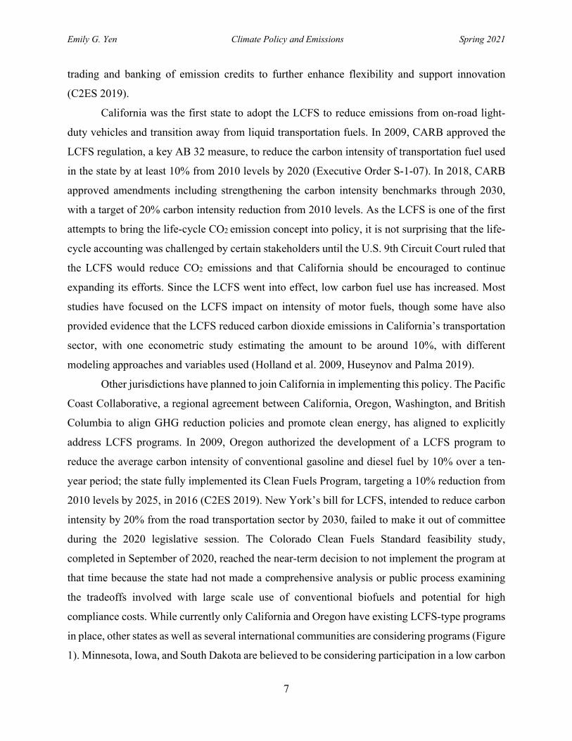
compliance costs. While currently only California and Oregon have existing LCFS-type programs
in place, other states as well as several international communities are considering programs (Figure
1). Minnesota, Iowa, and South Dakota are believed to be considering participation in a low carbon
Emily G. Yen Climate Policy and Emissions Spring 2021
8
fuel program tailored for Midwestern state needs specifically. Low carbon fuel mandates similar
to California’s LCFS have been adopted by the Environmental Protection Agency and other
jurisdictions including the European Union and the United Kingdom (CARB 2020).
Figure 1. States which have implemented or considered LCFS policies. Oregon fully implemented its Clean Fuels Program in 2016. The Pacific Coast Collaborative, a regional agreement between California, Oregon, Washington, and British Columbia to align GHG reduction policies and promote clean energy, has aligned to explicitly address LCFS programs. Minnesota, Iowa, and South Dakota are believed to be considering participation in a low carbon fuel program tailored for Midwestern state needs specifically. Colorado considered a Clean Fuels Standard. New York’s bill for LCFS failed to make it out of committee during the 2020 legislative session.
Econometric modeling
This study focused on modeling the impact of the LCFS on CO2 emissions for the
transportation sector. Population, affluence (GDP), and technology have been widely used in
literature to understand CO2 emission trends (Axsen et al. 2020, Lim and Won 2019). Carbon
dioxide emission in the U.S. can be explained by the STIRPAT model (STochastic Impacts by
Regression on Population, Affluence and Technology), which is an extension of the IPAT model
(the Impact on the environment depends on Population, Affluence, and Technology, or Impact =
Population × Affluence × Technology). The IPAT model can be used to analyze the effect of
economic activity on the environment. The STIRPAT model allows for the addition of statistical
Emily G. Yen Climate Policy and Emissions Spring 2021
9
assumptions and the testing of a hypothesis. Previous studies have also employed the synthetic
control method and the Lasso “post-double-selection” method. The Synthetic Control Method has
been utilized in environmental economics as it offers a framework to control unobservable time-
variant confounders. The Lasso method allows for validation of the choice of control variables and
can account for potential endogeneity in the policy treatment, specifically when there are concerns
regarding lags for control variables and their interactions with trends (Huseynov and Palma 2018).
In this study, I chose to approach the question of LCFS effectiveness through a difference-
in-differences (DID) econometric model and added different relevant variables used in other
models such as vehicle miles traveled (VMT), representing travel demand, falling under CEQA
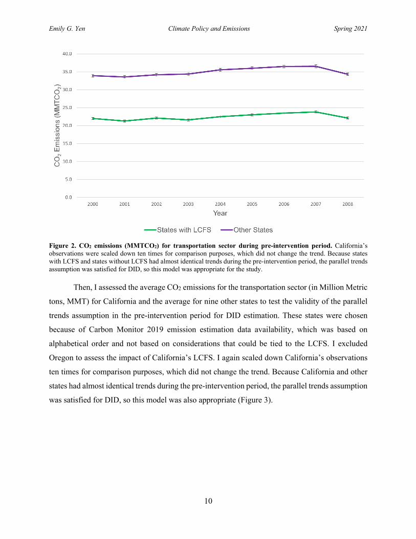
guidelines for conducting transportation analyses. First, I assessed the average CO2 emissions for
the transportation sector (in Million Metric tons, MMT) for California and Oregon and the average
for all other states to test the validity of the parallel trends assumption in the pre-intervention period
for DID estimation (Figure 2). In Oregon’s case, the period 2009-2016 could be considered an
“anticipatory” period and was deliberately included in the analysis due to 1) Oregon’s proximity
to California which approved its LCFS regulation in 2009, and 2) Oregon’s 2009 bill authorizing
the Oregon Environmental Quality Commission to adopt rules to reduce the average carbon
intensity of Oregon’s transportation fuels by 10% over a 10-year period before full implementation
of the program in 2016. I scaled down California’s observations ten times for comparison
purposes, which did not change the trend. Because states with LCFS and states without LCFS had
almost identical trends during the pre-intervention period, the parallel trends assumption was
satisfied for DID, so this model was appropriate for the study.
Emily G. Yen Climate Policy and Emissions Spring 2021
10
Figure 2. CO2 emissions (MMTCO2) for transportation sector during pre-intervention period. California’s observations were scaled down ten times for comparison purposes, which did not change the trend. Because states with LCFS and states without LCFS had almost identical trends during the pre-intervention period, the parallel trends assumption was satisfied for DID, so this model was appropriate for the study. Then, I assessed the average CO2 emissions for the transportation sector (in Million Metric
tons, MMT) for California and the average for nine other states to test the validity of the parallel
trends assumption in the pre-intervention period for DID estimation. These states were chosen
because of Carbon Monitor 2019 emission estimation data availability, which was based on
alphabetical order and not based on considerations that could be tied to the LCFS. I excluded
Oregon to assess the impact of California’s LCFS. I again scaled down California’s observations
ten times for comparison purposes, which did not change the trend. Because California and other
states had almost identical trends during the pre-intervention period, the parallel trends assumption
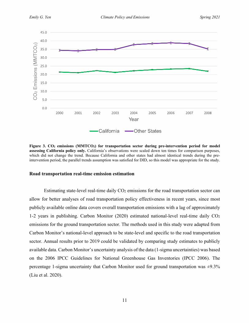
was satisfied for DID, so this model was also appropriate (Figure 3).
Emily G. Yen Climate Policy and Emissions Spring 2021
11
Figure 3. CO2 emissions (MMTCO2) for transportation sector during pre-intervention period for model assessing California policy only. California’s observations were scaled down ten times for comparison purposes, which did not change the trend. Because California and other states had almost identical trends during the pre-intervention period, the parallel trends assumption was satisfied for DID, so this model was appropriate for the study.
Road transportation real-time emission estimation
Estimating state-level real-time daily CO2 emissions for the road transportation sector can
allow for better analyses of road transportation policy effectiveness in recent years, since most
publicly available online data covers overall transportation emissions with a lag of approximately
1-2 years in publishing. Carbon Monitor (2020) estimated national-level real-time daily CO2
emissions for the ground transportation sector. The methods used in this study were adapted from
Carbon Monitor’s national-level approach to be state-level and specific to the road transportation
sector. Annual results prior to 2019 could be validated by comparing study estimates to publicly
available data. Carbon Monitor’s uncertainty analysis of the data (1-sigma uncertainties) was based
on the 2006 IPCC Guidelines for National Greenhouse Gas Inventories (IPCC 2006). The
percentage 1-sigma uncertainty that Carbon Monitor used for ground transportation was ±9.3%
(Liu et al. 2020).
CO
2 Em
issi
ons
(MM
TCO
2)
Emily G. Yen Climate Policy and Emissions Spring 2021
12
METHODS
Study sites
I obtained data for 27 U.S. states with mid-term or long-term emission reduction targets.
Historical GHG emission data spanned the period 1990-2017. Mid-term targets included the period
2020-2030 and long-term targets included years after 2030. I collected panel data for 50 U.S. states
with and without the LCFS policy for the period 2000-2018.
Data collection
I collected policy and target information including dates enacted for 27 states with emission
reduction targets and for LCFS policies for the period 2000-2017 from the U.S. Climate Alliance
(USCA), online publicly available information from state agencies, the Center for Climate and
Energy Solutions (C2ES), and the Database of State Incentives for Renewables & Efficiency
(DSIRE). I also collected data on transportation sector CO2 emissions, end of year population,
GDP percent change, and vehicle miles traveled (VMT) for 50 states in the period 2000-2017. I
collected state-level publicly available online transportation CO2 emissions data (MMT) and
historical GHG emissions data for 1990-2017 from the U.S. EIA, population data from the World
Population Review, gasoline tax data from the U.S. Department of Transportation Federal
Highway Administration, VMT data from the Eno Center for Transportation, and GDP growth
data from the U.S. Bureau of Economic Analysis (BEA). State-level monthly energy consumption
data, the prime supplier sales volumes of motor gasoline and diesel, were obtained from the U.S.
EIA Petroleum & Other Liquids. State-level daily indicators, the distance traveled, were obtained
from Trips by Distance data from Bureau of Transportation Statistics. This included the number
of trips made involving a stay of longer than 10 minutes at a location away from home.
State target analysis
To assess state-level ambition to reduce emissions, I compared state GHG emission
reduction targets. I grouped cities by target years and converted emission reduction targets to the
Emily G. Yen Climate Policy and Emissions Spring 2021
13
2005 baseline to compare target ambition across states. I categorized state targets by timeframe
and type to highlight levels of commitment. Mid-term and long-term emission reduction targets
alongside historical emission data provided a visualization of state target ambition timelines. The
analysis in this study relied on unadjusted values rather than considering the adjustment factor,
which the EIA introduced to match U.S. national total emissions by distributing to states in
proportion to each state’s share of the total emissions. Since some state-level carbon neutrality
targets are defined in terms of total GHG emissions rather than CO2 emissions, and as the focus of
this research did not involve providing a single definition of carbon neutrality, all state-level
carbon neutrality, net-zero, and GHG neutrality target values were considered as 100% GHG
emission reduction goals. State net-zero targets that include offsetting were graphed without the
offsetting portion. Due to the uncertainty in the accounting of LULUCF emissions, I excluded this
sector from emissions levels. Carbon neutrality and GHG neutrality targets take into account
projections and scenarios for LULUCF emissions, mostly CO2, meaning that there exists a level
of uncertainty surrounding the precise level of mid-century emissions under a carbon or GHG
neutrality target expressed excluding LULUCF.
Econometric analysis
To examine the impact of the LCFS on CO2 emissions from the transportation sector, the
dependent variable, I used a DID model and panel data for U.S. states for the period of 2000–2017
clustered at the state level (Eq. 1).
Eq. 1 Cit = β1 + β2LCFSi + β3postt + β4(LCFS × post)it + β5Xit + δit
In this regression, Cit is the dependent component, or million metric tons (MMT) of CO2 emitted
from the transportation sector; β1 is the intercept; LCFSi is a policy indicator for the existence of
the LCFS for state i with the β2 coefficient; postt indicates post-treatment period with the β3
coefficient; Xit is a vector of control variables; δit represents state-time random effects; and β4 is
the coefficient of interest for the interaction term. The timeframe for this study included the period
2000-2017 because of data availability for vehicle miles travelled (VMT) and gasoline tax.
California and Oregon are the only states which experience the LCFS policy or announcement in
2009. In both models, I controlled for VMT per capita; gasoline tax in cents per gallon; GDP
Emily G. Yen Climate Policy and Emissions Spring 2021
14
growth, or percent change; and population. I analyzed states with the policy and states without the
policy using Stata 16 (StataCorp 2019). In my models, I included three specifications. The first
specification included only the policy variable as the independent variable to pick up the impact
of state policy in the absence of the business-as-usual trajectory created by control variables, which
are key to removing confounding factors. The second specification included all variables. The third
specification excluded the states that intended to adopt similar laws: Colorado, Iowa, Minnesota,
New York, South Dakota, and Washington, assuming that observations for each remaining state
were independent. By excluding these states, any anticipatory effects prior to policy enactment
were avoided (Huseynov and Palma 2018). I clustered observations by state, expecting
observations to be correlated in the same cluster and independent across clusters. The first model
considered the impacts of California’s LCFS and Oregon’s standard, using panel data for 50 states.
I included Oregon’s 2009-2016 anticipatory period in the analysis for the first model. The second
model considered the impacts of only California’s LCFS, using panel data for 10 states. I used a
subset of states because they had 2019 estimated CO2 data and my main objective was to later use
this second model to show how estimated data could aid policy effectiveness assessments.
Emission estimation
To further evaluate the effectiveness of the LCFS in reducing state-level CO2 emissions
for the transportation sector, I estimated state-level real-time daily CO2 emissions for California’s
road transportation sector. Daily emissions estimates can be produced for this sector based on
regularly updated activity data, made possible by the availability of recent transport activity data.
I disaggregated the annual total state-level CO2 emissions for the transportation sector in 2018,
obtained from U.S. EIA and based on the EIA’s comprehensive state-level annual estimates of
energy consumption by sector and source, into the monthly data for the sector based on state-level
monthly activity data (Eq. 2).
Eq. 2 𝐸𝐸𝐸𝐸𝐸𝐸𝐸𝐸𝑚𝑚𝑚𝑚𝑚𝑚𝑚𝑚ℎ𝑙𝑙𝑙𝑙,2018 = 𝐸𝐸𝐸𝐸𝐸𝐸𝐸𝐸𝑙𝑙𝑦𝑦𝑦𝑦𝑦𝑦𝑙𝑙𝑙𝑙,2018 ∙
𝐴𝐴𝐴𝐴𝑚𝑚𝑚𝑚𝑚𝑚𝑚𝑚ℎ𝑙𝑙𝑙𝑙,2018
𝐴𝐴𝐴𝐴𝑙𝑙𝑦𝑦𝑦𝑦𝑦𝑦𝑙𝑙𝑙𝑙,2018
I estimated state-level road transportation CO2 monthly emissions (Emis) in 2019 based on the
change of monthly energy consumption data (activity data, AD) in 2019 compared to the same
period in 2018, assuming that the corresponding emission factors (EF) remained unchanged (Eq.
Emily G. Yen Climate Policy and Emissions Spring 2021
15
3). Carbon Monitor (2020) assumed that the daily variation of emissions was driven by activity
data and the contribution from emission factors was negligible since they evolve at longer
timescales due to policy implementation and technology shifts. State-level monthly energy
consumption data was comprised of the prime supplier sales volumes of motor gasoline in
thousand gallons per day.
Eq. 3 𝐸𝐸𝐸𝐸𝐸𝐸𝐸𝐸 = ∑∑∑𝐴𝐴𝐴𝐴𝑖𝑖,𝑘𝑘 ∙ 𝐸𝐸𝐸𝐸𝑖𝑖,𝑘𝑘
Here, i refers to region and k refers to fuel type. EF is comprised of the net heating values (v) for
each fuel type in terms of energy obtained per unit of fuel; the carbon content (c) per energy output
in units of t C/TJ; and the oxidation rate (o), or the percent fraction of fuel oxidized during
combustion (Eq. 4).
Eq. 4 𝐸𝐸𝐸𝐸𝐸𝐸𝐸𝐸 = ∑∑∑𝐴𝐴𝐴𝐴𝑖𝑖,𝑘𝑘 ∙ (𝑣𝑣𝑖𝑖,𝑘𝑘 ∙ 𝑐𝑐𝑖𝑖,𝑘𝑘 ∙ 𝑜𝑜𝑖𝑖,𝑘𝑘)
I added monthly emissions for 2019 and allocated yearly emissions for the sector to each day using
state-level daily indicators, comprised of Trips by Distance traveled data, assuming that emission
factors remained unchanged in 2019 (Eq. 5).
Eq. 5 𝐸𝐸𝐸𝐸𝐸𝐸𝐸𝐸𝑑𝑑𝑦𝑦𝑖𝑖𝑙𝑙𝑙𝑙,2019 = 𝐸𝐸𝐸𝐸𝐸𝐸𝐸𝐸𝑙𝑙𝑦𝑦𝑦𝑦𝑦𝑦𝑙𝑙𝑙𝑙,2019 ∙
𝐴𝐴𝐴𝐴𝑑𝑑𝑦𝑦𝑖𝑖𝑙𝑙𝑙𝑙,2019
𝐴𝐴𝐴𝐴𝑙𝑙𝑦𝑦𝑦𝑦𝑦𝑦𝑙𝑙𝑙𝑙,2019
To validate results, I compared the estimated 2018 annual emissions to EIA 2018 emissions data.
To demonstrate the viability of using state-level near-real-time daily CO2 emission data in
assessing the effectiveness of the LCFS for the period 2000-2019, I applied the California 2019
road transportation sector data estimated in this study to Equation 1. I used 2018 EIA data for
emissions from the transportation sector and excluded the year 2020 due to changes in the road
transportation sector during COVID-19. This exclusion also makes sense since California’s
original LCFS goal in 2009 used 2020 as the target year. Due to data availability issues, I used
2017 data for gasoline tax and VMT in the 2018-2019 period and used Carbon Monitor estimated
data for nine other states. I considered the (1) CA Policy Only; (2) All Ten States Included; and
(3) Colorado Excluded specifications, mirroring the earlier methods in the first model, to assess
the impact of California’s LCFS on CO2 emissions for an extended and more recent post-
intervention timeframe. This model excluded Oregon and focused on the impact of California’s
LCFS.
Emily G. Yen Climate Policy and Emissions Spring 2021
16
RESULTS
Data summary
There were 900 observations in the dataset for the first econometric model and 200
observations for the second. California’s population steadily increased over the observed
timeframe. Transportation emissions declined over the period 2007-2013, followed by annual
increases through 2017. Diesel fuel blend sales decreased by 50 million gallons; sale and blending
of biodiesel and renewable diesel increased by more than 60 million gallons; and emissions from
gasoline used in on-road passenger cars, trucks, and SUVs were the main driver of the increases
between 2013 and 2017, making up 74% of transportation emissions. Biodiesel and renewable
diesel percentages in the total diesel blend increased from 0.5% to 18.5% over the period 2011-
2018 in large part because of the LCFS. For the period 2000-2018, the carbon intensity of
California’s economy decreased by 43% and the state’s GDP increased by 59% (CARB 2018).
California managed to push its per capita VMT averages below the national average for the period
2001-2017; while the state’s per capita VMT generally decreased over this time period, it increased
between 2012 and 2016. State-level monthly energy consumption data- the prime supplier sales
volumes of motor gasoline- decreased in 2020 during the COVID-19 period (EIA 2021).
State target analysis
I found that California’s targets were generally more ambitious than other state-level
targets. For both mid-term (2020-2030) and long-term (post 2030) targets, I documented a greater
amount of legislation than executive orders, announced plans, or recommended goals (Appendix
Table 1). Binding commitments were generally greater in the West Coast and Northeast regions,
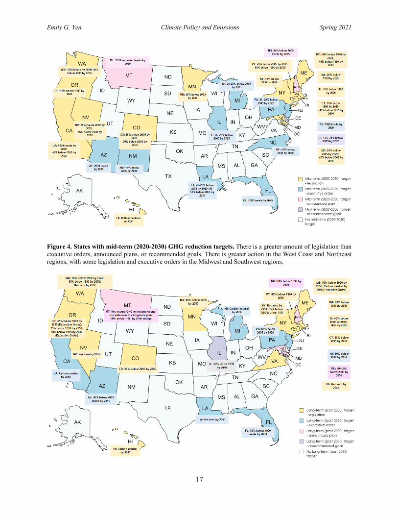
with some legislation and executive orders in the Midwest and Southwest regions (Figures 4 and
5).
Emily G. Yen Climate Policy and Emissions Spring 2021
17
Figure 4. States with mid-term (2020-2030) GHG reduction targets. There is a greater amount of legislation than executive orders, announced plans, or recommended goals. There is greater action in the West Coast and Northeast regions, with some legislation and executive orders in the Midwest and Southwest regions.
Emily G. Yen Climate Policy and Emissions Spring 2021
18
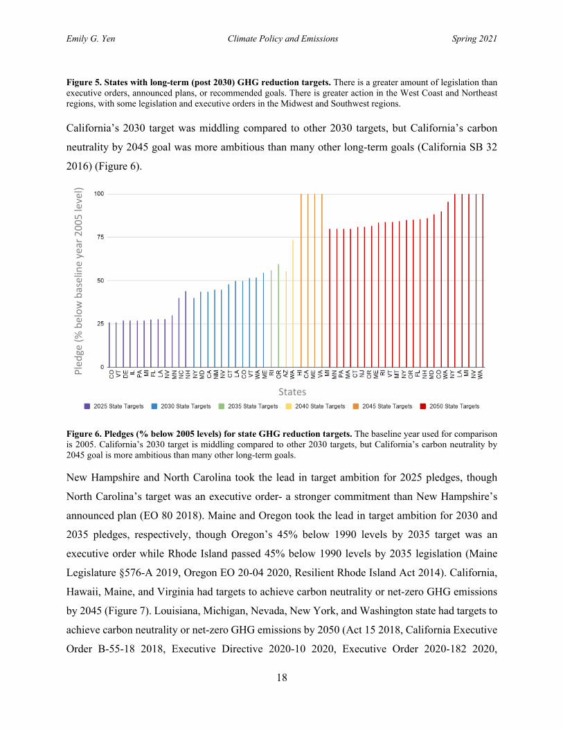
Figure 5. States with long-term (post 2030) GHG reduction targets. There is a greater amount of legislation than executive orders, announced plans, or recommended goals. There is greater action in the West Coast and Northeast regions, with some legislation and executive orders in the Midwest and Southwest regions. California’s 2030 target was middling compared to other 2030 targets, but California’s carbon
neutrality by 2045 goal was more ambitious than many other long-term goals (California SB 32
2016) (Figure 6).
Figure 6. Pledges (% below 2005 levels) for state GHG reduction targets. The baseline year used for comparison is 2005. California’s 2030 target is middling compared to other 2030 targets, but California’s carbon neutrality by 2045 goal is more ambitious than many other long-term goals. New Hampshire and North Carolina took the lead in target ambition for 2025 pledges, though
North Carolina’s target was an executive order- a stronger commitment than New Hampshire’s
announced plan (EO 80 2018). Maine and Oregon took the lead in target ambition for 2030 and
2035 pledges, respectively, though Oregon’s 45% below 1990 levels by 2035 target was an
executive order while Rhode Island passed 45% below 1990 levels by 2035 legislation (Maine
Legislature §576-A 2019, Oregon EO 20-04 2020, Resilient Rhode Island Act 2014). California,
Hawaii, Maine, and Virginia had targets to achieve carbon neutrality or net-zero GHG emissions
by 2045 (Figure 7). Louisiana, Michigan, Nevada, New York, and Washington state had targets to
achieve carbon neutrality or net-zero GHG emissions by 2050 (Act 15 2018, California Executive
Order B-55-18 2018, Executive Directive 2020-10 2020, Executive Order 2020-182 2020,
Ple
dge
(% b
elow
bas
elin
e ye
ar 2
005
leve
l)
States
Emily G. Yen Climate Policy and Emissions Spring 2021
19
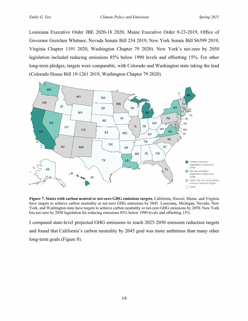
Louisiana Executive Order JBE 2020-18 2020, Maine Executive Order 9-23-2019, Office of
Governor Gretchen Whitmer, Nevada Senate Bill 254 2019, New York Senate Bill S6599 2019,
Virginia Chapter 1191 2020, Washington Chapter 79 2020). New York’s net-zero by 2050
legislation included reducing emissions 85% below 1990 levels and offsetting 15%. For other
long-term pledges, targets were comparable, with Colorado and Washington state taking the lead
(Colorado House Bill 19-1261 2019, Washington Chapter 79 2020).
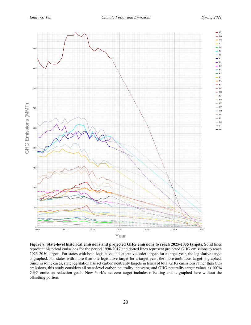
Figure 7. States with carbon neutral or net-zero GHG emissions targets. California, Hawaii, Maine, and Virginia have targets to achieve carbon neutrality or net-zero GHG emissions by 2045. Louisiana, Michigan, Nevada, New York, and Washington state have targets to achieve carbon neutrality or net-zero GHG emissions by 2050. New York has net-zero by 2050 legislation for reducing emissions 85% below 1990 levels and offsetting 15%. I compared state-level projected GHG emissions to reach 2025-2050 emission reduction targets
and found that California’s carbon neutrality by 2045 goal was more ambitious than many other
long-term goals (Figure 8).
Emily G. Yen Climate Policy and Emissions Spring 2021
20
Figure 8. State-level historical emissions and projected GHG emissions to reach 2025-2035 targets. Solid lines represent historical emissions for the period 1990-2017 and dotted lines represent projected GHG emissions to reach 2025-2050 targets. For states with both legislative and executive order targets for a target year, the legislative target is graphed. For states with more than one legislative target for a target year, the more ambitious target is graphed. Since in some cases, state legislation has set carbon neutrality targets in terms of total GHG emissions rather than CO2 emissions, this study considers all state-level carbon neutrality, net-zero, and GHG neutrality target values as 100% GHG emission reduction goals. New York’s net-zero target includes offsetting and is graphed here without the offsetting portion.
Year
GH
G E
mis
sion
s (M
MT)
Emily G. Yen Climate Policy and Emissions Spring 2021
21
Econometric analysis
When estimating the effect of California’s LCFS on transportation CO2 emissions for the
period 2000-2017 using panel data for 50 states, the results predicted that the adoption of the LCFS
decreased state CO2 transportation emissions by approximately 22.9 MMT with a standard error
of 2.32. The magnitude of the reduction represented around 10.5% of transportation CO2 emissions
from California in 2017. As these results only slightly exceeded the previous literature results of a
21.2 MMT reduction, I determined my model and variables to be appropriate for further analyses
(Appendix Table 2).
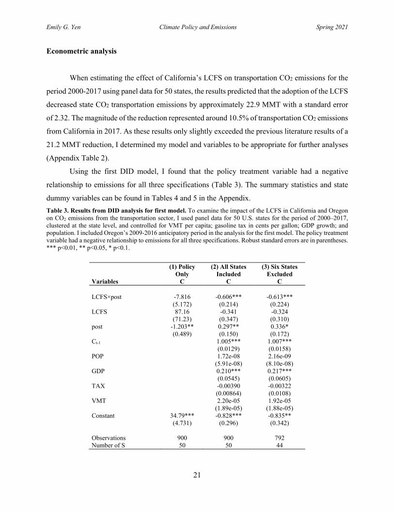
Using the first DID model, I found that the policy treatment variable had a negative
relationship to emissions for all three specifications (Table 3). The summary statistics and state
dummy variables can be found in Tables 4 and 5 in the Appendix. Table 3. Results from DID analysis for first model. To examine the impact of the LCFS in California and Oregon on CO2 emissions from the transportation sector, I used panel data for 50 U.S. states for the period of 2000–2017, clustered at the state level, and controlled for VMT per capita; gasoline tax in cents per gallon; GDP growth; and population. I included Oregon’s 2009-2016 anticipatory period in the analysis for the first model. The policy treatment variable had a negative relationship to emissions for all three specifications. Robust standard errors are in parentheses. *** p<0.01, ** p<0.05, * p<0.1.
(1) Policy Only
(2) All States Included
(3) Six States Excluded
Variables C C C LCFS×post -7.816 -0.606*** -0.613*** (5.172) (0.214) (0.224) LCFS 87.16 -0.341 -0.324 (71.23) (0.347) (0.310) post -1.203** 0.297** 0.336* (0.489) (0.150) (0.172) Ct-1 1.005*** 1.007*** (0.0129) (0.0158) POP 1.72e-08 2.16e-09 (5.91e-08) (8.10e-08) GDP 0.210*** 0.217*** (0.0545) (0.0605) TAX -0.00390 -0.00322 (0.00864) (0.0108) VMT 2.20e-05 1.92e-05 (1.89e-05) (1.88e-05) Constant 34.79*** -0.828*** -0.835** (4.731) (0.296) (0.342) Observations 900 900 792 Number of S 50 50 44
Emily G. Yen Climate Policy and Emissions Spring 2021
22
The specification in Column 2 of Table 3, which included controls and all states, predicted that the
adoption of the LCFS decreased state CO2 transportation emissions by approximately 0.61 MMT
with a standard error of 0.21. A one sample standard deviation increase led to an increase of 0.21
standard deviations in emissions, ceteris paribus. The magnitude of the reduction represented
around 0.03% of transportation CO2 emissions from the U.S. and around 0.26% of transportation
CO2 emissions from states with LCFS in 2017. In specifications 2 and 3, GDP growth had a
positive relationship to emissions (p<0.01); population and VMT had positive relationships to
emissions; and gasoline tax had a negative relationship to emissions. The coefficient for
LCFSXpost had a negative relationship to emissions (p<0.01). After excluding states which
considered adopting similar policies from the regression, the coefficient for LCFSXpost in Column
3 was similar to the coefficient for LCFSXpost in Column 2. The first specification, which did not
include controls, produced a different result. Focusing on the two specifications with controls, I
concluded that the result was robust since the coefficients both had a negative relationship to
emissions (p<0.01).
Using the second DID model, I found that the policy treatment variable had a negative
relationship to emissions (p<0.01) for all three specifications (Table 6). The summary statistics
and state dummy variables can be found in Tables 7 and 8 in the Appendix. The specification in
Column 2 of Table 6, which included controls and all ten states, predicted that California’s
adoption of the LCFS decreased state CO2 transportation emissions by approximately 15.1 MMT
with a standard error of 2.82. The magnitude of the reduction represented around 6.95% of
transportation CO2 emissions from California in 2017. In specifications 2 and 3, GDP growth had
a positive relationship to emissions (p<0.05); population had a positive relationship to emissions
(p<0.01); VMT had a positive relationship to emissions (p<0.01); and gasoline tax had a negative
relationship to emissions (p<0.01). The coefficient for LCFSXpost had a negative relationship to
emissions (p<0.01) for all three specifications. After excluding Colorado, which considered
adopting a similar policy, the coefficient for LCFSXpost in Column 3 was close to the coefficient
for LCFSXpost in Column 2. Focusing on the two specifications with controls, I concluded that
the result was robust since the coefficients both had a negative relationship to emissions (p<0.01).
Emily G. Yen Climate Policy and Emissions Spring 2021
23
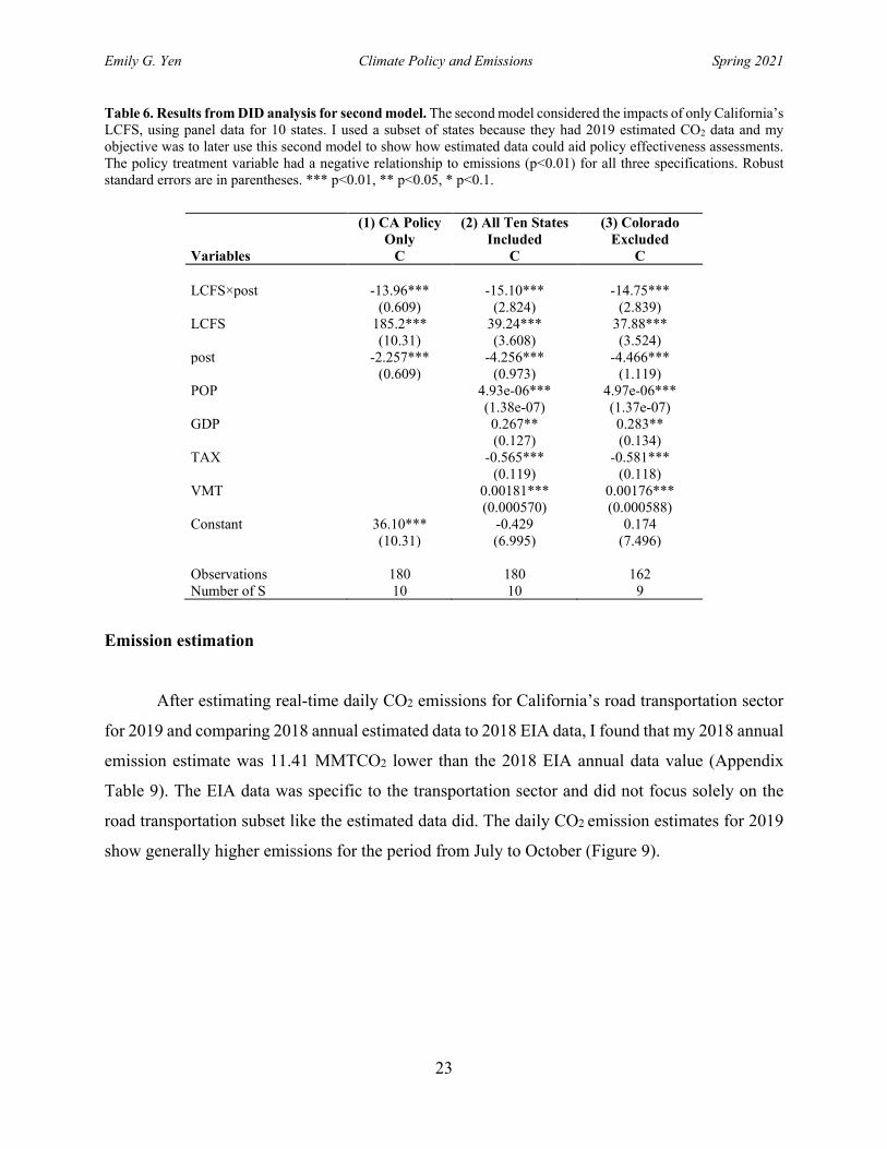
Table 6. Results from DID analysis for second model. The second model considered the impacts of only California’s LCFS, using panel data for 10 states. I used a subset of states because they had 2019 estimated CO2 data and my objective was to later use this second model to show how estimated data could aid policy effectiveness assessments. The policy treatment variable had a negative relationship to emissions (p<0.01) for all three specifications. Robust standard errors are in parentheses. *** p<0.01, ** p<0.05, * p<0.1.
(1) CA Policy Only
(2) All Ten States Included
(3) Colorado Excluded
Variables C C C LCFS×post -13.96*** -15.10*** -14.75*** (0.609) (2.824) (2.839) LCFS 185.2*** 39.24*** 37.88*** (10.31) (3.608) (3.524) post -2.257*** -4.256*** -4.466*** (0.609) (0.973) (1.119) POP 4.93e-06*** 4.97e-06*** (1.38e-07) (1.37e-07) GDP 0.267** 0.283** (0.127) (0.134) TAX -0.565*** -0.581*** (0.119) (0.118) VMT 0.00181*** 0.00176*** (0.000570) (0.000588) Constant 36.10*** -0.429 0.174 (10.31) (6.995) (7.496) Observations 180 180 162 Number of S 10 10 9
Emission estimation
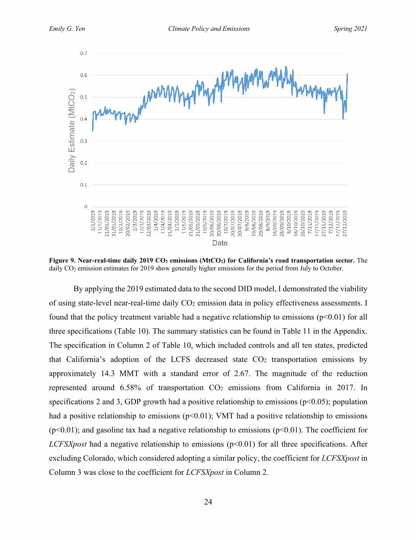
After estimating real-time daily CO2 emissions for California’s road transportation sector
for 2019 and comparing 2018 annual estimated data to 2018 EIA data, I found that my 2018 annual
emission estimate was 11.41 MMTCO2 lower than the 2018 EIA annual data value (Appendix
Table 9). The EIA data was specific to the transportation sector and did not focus solely on the
road transportation subset like the estimated data did. The daily CO2 emission estimates for 2019
show generally higher emissions for the period from July to October (Figure 9).
Emily G. Yen Climate Policy and Emissions Spring 2021
24
Figure 9. Near-real-time daily 2019 CO2 emissions (MtCO2) for California’s road transportation sector. The daily CO2 emission estimates for 2019 show generally higher emissions for the period from July to October.
By applying the 2019 estimated data to the second DID model, I demonstrated the viability
of using state-level near-real-time daily CO2 emission data in policy effectiveness assessments. I
found that the policy treatment variable had a negative relationship to emissions (p<0.01) for all
three specifications (Table 10). The summary statistics can be found in Table 11 in the Appendix.
The specification in Column 2 of Table 10, which included controls and all ten states, predicted
that California’s adoption of the LCFS decreased state CO2 transportation emissions by
approximately 14.3 MMT with a standard error of 2.67. The magnitude of the reduction
represented around 6.58% of transportation CO2 emissions from California in 2017. In
specifications 2 and 3, GDP growth had a positive relationship to emissions (p<0.05); population
had a positive relationship to emissions (p<0.01); VMT had a positive relationship to emissions
(p<0.01); and gasoline tax had a negative relationship to emissions (p<0.01). The coefficient for
LCFSXpost had a negative relationship to emissions (p<0.01) for all three specifications. After
excluding Colorado, which considered adopting a similar policy, the coefficient for LCFSXpost in
Column 3 was close to the coefficient for LCFSXpost in Column 2.
Dai
ly E
stim
ate
(MtC
O2)
Emily G. Yen Climate Policy and Emissions Spring 2021
25
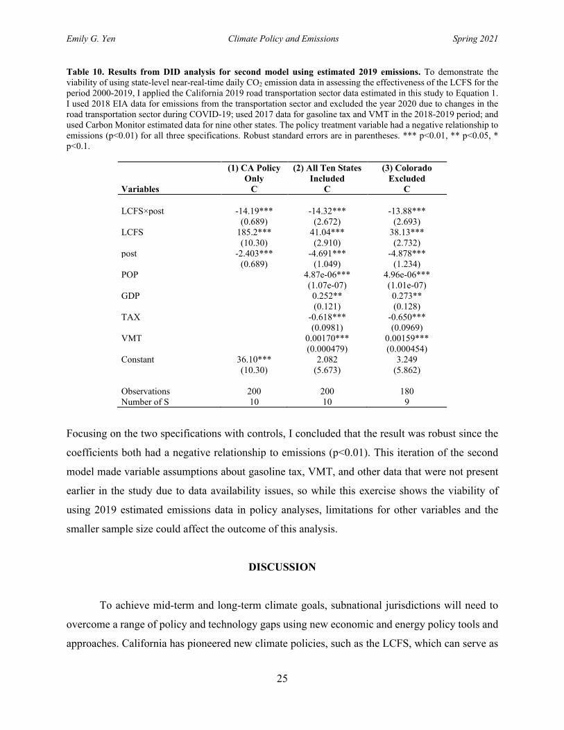
Table 10. Results from DID analysis for second model using estimated 2019 emissions. To demonstrate the viability of using state-level near-real-time daily CO2 emission data in assessing the effectiveness of the LCFS for the period 2000-2019, I applied the California 2019 road transportation sector data estimated in this study to Equation 1. I used 2018 EIA data for emissions from the transportation sector and excluded the year 2020 due to changes in the road transportation sector during COVID-19; used 2017 data for gasoline tax and VMT in the 2018-2019 period; and used Carbon Monitor estimated data for nine other states. The policy treatment variable had a negative relationship to emissions (p<0.01) for all three specifications. Robust standard errors are in parentheses. *** p<0.01, ** p<0.05, * p<0.1.
(1) CA Policy Only
(2) All Ten States Included
(3) Colorado Excluded
Variables C C C LCFS×post -14.19*** -14.32*** -13.88*** (0.689) (2.672) (2.693) LCFS 185.2*** 41.04*** 38.13*** (10.30) (2.910) (2.732) post -2.403*** -4.691*** -4.878*** (0.689) (1.049) (1.234) POP 4.87e-06*** 4.96e-06*** (1.07e-07) (1.01e-07) GDP 0.252** 0.273** (0.121) (0.128) TAX -0.618*** -0.650*** (0.0981) (0.0969) VMT 0.00170*** 0.00159*** (0.000479) (0.000454) Constant 36.10*** 2.082 3.249 (10.30) (5.673) (5.862) Observations 200 200 180 Number of S 10 10 9
Focusing on the two specifications with controls, I concluded that the result was robust since the
coefficients both had a negative relationship to emissions (p<0.01). This iteration of the second
model made variable assumptions about gasoline tax, VMT, and other data that were not present
earlier in the study due to data availability issues, so while this exercise shows the viability of
using 2019 estimated emissions data in policy analyses, limitations for other variables and the
smaller sample size could affect the outcome of this analysis.
DISCUSSION
To achieve mid-term and long-term climate goals, subnational jurisdictions will need to
overcome a range of policy and technology gaps using new economic and energy policy tools and
approaches. California has pioneered new climate policies, such as the LCFS, which can serve as
Emily G. Yen Climate Policy and Emissions Spring 2021
26
a reference point for the implementation of other state and federal policies (Mazmanian et al.
2020). These efforts must be matched with scientific approaches to assess mitigation strategies,
document progress, and highlight implications for improvement (Hsu et al. 2019). Assessing the
ambition and stringency of state targets as well as the effectiveness of policies can provide useful
insights for other states considering similar strategies. It is essential to understand LCFS policy
effectiveness because the main reason for the policy’s legal support was a high expectation of CO2
emission reduction. LCFS-type policies have not been widely researched using econometric
methods since they are still relatively new (Huseynov and Palma 2018). Furthermore, previous
LCFS policy research has not applied real-time CO2 emission estimates to assess effectiveness
over a more recent timeframe. I addressed these research gaps to inform the discussion surrounding
climate targets and policy to reach Paris Agreement and carbon neutrality goals. By analyzing the
ambition and stringency of state-level climate targets, assessing the effectiveness of one of
California’s most significant road transportation policies, and utilizing real-time emission
estimates in analysis, I aimed to highlight existing potential gaps to achieve climate goals. Drawing
on California’s framework, U.S. states can increase emission reduction target stringency and
ambition by passing legislation or executive orders to achieve mid-century carbon neutrality. The
significant impact that the LCFS has had in reducing CO2 emissions in the transportation sector
underlines the effectiveness of this policy, which can serve as a reference point for future
implementation by other states. Using the 2019 estimated data for real-time daily CO2 emissions
for the road transportation sector in an econometric model supported my argument for LCFS
effectiveness and illustrated the usefulness of exploring different methods of emission estimation
in transportation policy analyses. Daily near-real-time emissions data could aid future scientific
research in this critical sector (Liu et al. 2020).
State target analysis
The comparison of state-level mid-term and long-term emission reduction targets suggests
that states can increase stringency by adopting more legislation over executive orders, announced
plans, or recommended targets. That there is a greater amount of legislation than executive orders,
announced plans, and recommended goals for both mid-term (2020-2030) and long-term (post
2030) state targets shows that state-level targets are generally binding. It is notable that
Emily G. Yen Climate Policy and Emissions Spring 2021
27
commitment levels are generally higher in the West Coast and Northeast regions, with some
legislation and executive orders in the Southwest and Midwest regions. These regions may have
greater commitments because they contain more states in the U.S. Climate Alliance, which
requires commitments from member states to implement policies that advance the goals of the
Paris Agreement by reducing GHG emissions by at least 26-28% below 2005 levels by 2025
(USCA 2020). Most states with mid-term targets also have long-term targets, suggesting that the
general climate framework includes interim targets along with longer-term goals. There are fewer
state targets for the period 2030-2045, which falls into the long-term category for this study,
showing a potential opportunity to set more interim benchmarks and long-term targets to increase
accountability. Washington, for example, has set targets for 2020, 2030, 2040, and 2050, as well
as a net-zero mid-century target (Washington Chapter 79 2020). California’s targets are similarly
spread out, spanning 2020, 2030, and carbon neutrality by 2045 (California Executive Order B-
55-18). Washington’s targets are generally on the ambitious end of the spectrum for each target
year and California’s 2045 target outstrips many other long-term mid-century targets,
demonstrating that interim benchmarks paired with ambitious longer-term goals can provide a
roadmap for accelerated emission reduction.
The comparison of state-level mid-term and long-term emission reduction targets also
reveals that states would be able to increase ambition by pledging mid-century carbon neutrality
or net-zero long-term targets. Apart from the nine states which have pledged carbon neutrality or
net-zero GHG emissions, most states with long-term targets have set comparable 2050 goals.
Potential reasons for this might include the benefits of common milestones, which can provide
clear policy signals and drive down costs; dialogue and technical exchange, which can create
shared understanding of technology pathways and implementation experience; and state
leadership, which can promote pioneering solutions and seek to align state-level interests. The
states which have set more ambitious targets often have the authority to act independently within
the U.S. system; have administrative and technical capacity to create pioneering policies; and have
had historical success in tackling effective implementation (Mazmanian et al. 2020). As the 2050
targets generally aim for over 74% reductions below 2005 emissions levels, further ambition
would involve establishing mid-century 100% GHG emission reduction targets or carbon
neutrality goals. In the mid-term, greater ambition for concrete action can continue to support the
pathway towards longer-term goals. Pursuing greater ambition requires a consistent reporting
Emily G. Yen Climate Policy and Emissions Spring 2021
28
framework that captures both quantitative and qualitative aspects of state actions, as well as greater
attention paid to implementation of subnational climate policies (Chan et al. 2015, Hsu et al. 2018).
The comparison of state-level mid-term and long-term emission reduction targets indicates
that California’s mid-term legislation to reduce emissions and long-term executive order to achieve
carbon neutrality by 2045 can serve as a framework for subnational action (Lim and Won 2019,
Sperling and Eggert 2014). California has often used executive authority to drive groundbreaking
climate policy work, later codifying longer-term goals through legislation. The state has also built
in mechanisms for continuous improvement; for example, when the 2045 carbon neutrality order
was released, the state had recently achieved its 2020 target. If the state kept its goal of achieving
the 2050 target, based on projected emission trajectory, it would have implied a slowdown in the
rate of emission reduction between 2030 and 2050. Finally, in its effort to achieve long-term goals
such as carbon neutrality, the state has employed a variety of emission reduction strategies. Other
studies aiming to inform the discussion on carbon neutrality have focused on emission reduction
in different sectors of the energy economy, exploring the unexpected synergies, counterintuitive
results, and tradeoffs involved with reaching long-term goals (IPCC 2018, Larson et al. 2020,
Mahone et al. 2020, Williams et al. 2021). These studies acknowledge that advanced mitigation
strategies and early emission reduction targets can support potential carbon neutrality pathways
(Mahone et al. 2020). California’s mid-term and long-term targets are stringent and ambitious-
undoubtedly necessary elements of the state’s overall climate strategy.
Econometric analysis
The model results in this study demonstrated that the LCFS has greatly impacted CO2
emission reduction in the transportation sector, though these analyses differ from the ones used by
Huseynov and Palma (2018). My analyses considered different variables and groupings; included
Oregon’s policy in the first model; looked at a more recent timeframe; and considered impacts on
transportation CO2 emissions specifically. I also incorporated road transportation sector near-real-
time emissions into the second model. These differences can account for varied results from
literature, but the overall trends remain the same. As expected, the adoption of the LCFS decreased
state emissions, performing best with controls present and states considering adopting similar
policies, with the potential for an anticipatory period prior to policy enactment, excluded from the
Emily G. Yen Climate Policy and Emissions Spring 2021
29
regression (Huseynov and Palma 2018). The results from the first model suggest that California
and Oregon policy impacts may need to be examined separately, or that more research can be done
to assess anticipatory period effects. The results from both models suggest that the LCFS on its
own is not a silver bullet policy for addressing transportation emissions. Policy mixes- a particular
strength of California’s climate approach- can ensure that balanced strategies tackle emission
reduction in various capacities. Certainly, the LCFS has great potential to play a major role in such
a policy mix. Overall, the results make sense in the context of previous literature, which found that
the LCFS is an effective policy for California’s transportation sector and that cross-sector
decarbonization is particularly reliant on the availability of low carbon fuels (Huseynov and Palma
2018, Mahone et al. 2020, Sperling 2016).
Emission estimation and analysis
The estimated annual 2018 data value for California’s road transportation sector was lower
than the EIA transportation data value, which followed expectations as the estimation focused on
road transportation, a subset of the transportation sector (Liu et al. 2020). Updating the estimated
daily dataset could offer a range of opportunities for related scientific research in the road
transportation sector specifically (Liu et al. 2020). The detail and timeliness of these types of
emissions estimates can facilitate more agile and adaptive management of CO2 emissions during
structural changes and the ongoing energy transition.
I demonstrated the viability of using my real-time 2019 emissions data estimate for
California, along with Carbon Monitor’s real-time data estimates for nine other states, to assess
LCFS effectiveness. The model results furthered my argument for LCFS effectiveness (Huseynov
and Palma 2018). My first model considered all U.S. states and a shorter timeframe; used different
variable data and only general transportation sector emissions data; and did not use 2019 road
transportation emissions estimates, while the second model included near-real-time road
transportation data for 2019 after emission estimation; considered ten U.S. states and a longer
timeframe including recent years; looked at California’s LCFS specifically, excluding Oregon’s
policy; and excluded fewer states in the third specification due to having a narrower scope. While
model differences and associated assumptions can account for the varied results from the first
model in this study and from earlier literature, overall trends remained the same; as expected,
Emily G. Yen Climate Policy and Emissions Spring 2021
30
California’s LCFS decreased state emissions, performing best with controls present. This result
makes sense in the context of previous literature and earlier results for this study, which found that
the LCFS is an effective policy. The coefficients for LCFSXpost in this iteration of the second
model were similar to the coefficients for LCFSXpost in the previous iteration. Results in this study
were lower than results found using other approaches (Huseynov and Palma 2018). Other models
with controls have previously predicted that the adoption of the California LCFS in the
transportation sector decreased emissions approximately 21.19 MMT for an earlier timeframe. All
models found the policy to be effective (Huseynov and Palma 2018, Mahone et al. 2020, Sperling
2016). Differences between results could be explained by the inherent difference between general
transportation sector emissions and the road transportation sector emissions subset as well as the
different model assumptions. The results from this model suggest that more research can be done
to apply recent CO2 emission estimates while taking into consideration data availability issues for
other variables. This exercise reveals that emissions estimates for recent years can be applied to
road transportation policy analyses (Liu et al. 2020). Real-time daily estimates can increase the
policy-relevance of subnational emissions monitoring, potentially moving up the timetable of
policy adjustments by roughly 1-2 years when compared to current available data for annual
emissions.
California climate policy for road transportation
In-depth analysis of California’s climate and road transportation policy microcosm can
influence decision-making on larger scales. California’s binding climate targets and policies are
especially critical for transportation analyses, as the state has tremendous opportunities for
reducing emissions in this sector (Mazmanian et al. 2020). The state’s binding long-term target to
achieve carbon neutrality by 2045 is more ambitious than the long-term targets of most other states.
After empirically measuring the effect of one of California’s major road transportation policies,
the LCFS, on transportation sector CO2 emissions, the impact is apparent and supports previous
findings (Huseynov and Palma 2018). Using an alternative method of estimating state-level real-
time CO2 emissions for the road transportation sector and then conducting policy analysis with
this data illustrates the opportunity for this data to be used as a tool in future assessments of climate
measures for road transportation. The results support the argument that California’s major climate
Emily G. Yen Climate Policy and Emissions Spring 2021
31
policy for the transportation sector is highly effective and that the state’s carbon neutrality target
can provide a framework for ambition in other jurisdictions. While it has previously been argued
that California is an outlier when it comes to environmental and energy policy, learning from
California’s experiences can still benefit future efforts if solid scientific approaches are used to
assess mitigation effort and highlight lessons learned (Hsu et al. 2019). The results of this study,
as well as future analyses in this field, can shed light on potential effective approaches in
transportation and energy regulation for other jurisdictions.
Limitations and areas for further study
The limitations of this study involve the boundaries drawn around data collection and
assumptions made in the analysis. For the first econometric model, I used publicly available data
ending with the year 2017 and used a set of controls and variables, basing model construction on
data availability and integral assumptions. For the second model using estimated emissions, further
assumptions were applied due to VMT and gasoline tax data availability issues for the 2018-2019
period. This model also used a subset of U.S. states, differing from the first model. Due to these
limitations, further work can be done in using econometric models and other methods to
understand LCFS effectiveness and inform future policy adjustments. Nevertheless, results from
econometric models can be useful because they can provide insights for future research directions
as well as potential lessons learned. The limitations and results offer considerations and
opportunities for further areas of research. Future research might analyze the potential interaction
of the LCFS with other related programs to improve understanding of the impacts of
complementary climate policies on state emissions. Other key topics could be explored including
the effects of the LCFS on green technology adoption and implementation or on health co-benefits
for heavily burdened communities with respect to environmental justice issues and equity
(Huseynov and Palma 2018, Mahone et al. 2020). As this study focuses on state-level policy and
emissions, a similar framework may be applied to other subnational jurisdictions with comparable
policies (Mazmanian et al. 2020).
Emily G. Yen Climate Policy and Emissions Spring 2021
32
Policy implications
As currently there is no general consensus on a theory for carbon neutrality or states action,
rigorous policy analyses are necessary to understand near-term priorities and longer-term pathways
to achieve climate goals. Comparing California’s climate targets with other state-level approaches
and assessing climate policy effectiveness using near-real-time emission data can inform future
policy directions. Dynamic information on CO2 emissions will be critical for understanding the
recent impacts of climate policies and potential for future action (Liu et al. 2020). Previous
literature has pointed out the necessity of quantifying CO2 reductions under low carbon standards
and has conducted first efforts at rigorous analysis (Huseynov and Palma 2018, Yeh et al. 2016).
This study builds on the literature by synthesizing and comparing state-level target data in a new
format to provide context for subnational action; applying different empirical models for policy
analysis; and constructing a novel dataset of daily 2019 CO2 emissions for California’s road
transportation sector, adapted from national-level methods in the literature. The results underscore
California’s long-term target ambition and LCFS policy effectiveness while offering a new tool
for future analyses. The ongoing target adjustments for both California’s emission reduction
targets and the LCFS reflect high adaptability and iterative increases in ambition as part of the
state’s climate policy framework. While environmental impact, or the effectiveness in reducing
emissions, is an important metric for policy evaluation, state-level climate policy implementation
needs to be evaluated based on other metrics as well: economic impact, or the extent of market
stimulation, and equity, including environmental justice concerns. As the U.S. re-engages with the
Paris Agreement and signals openness to pursuing a mid-century carbon neutrality goal, and as
subnational actors continue to drive actionable climate policy, empirical studies on established
targets for highly polluting sectors can clarify concrete near-term priorities and inform long-term
decarbonization strategies.
ACKNOWLEDGEMENTS
I am deeply grateful to my invaluable thesis mentor and research advisor, Dr. Fan Dai, whose
pioneering work in climate and energy policy inspired and guided my study. Her expertise and
resources greatly informed my approach, and I am fortunate to have had the opportunity to learn
Emily G. Yen Climate Policy and Emissions Spring 2021
33
from her. Carbon Monitor data and literature were instrumental to developing my methods. Thank
you to the researchers at the California-China Climate Institute for feedback on data visualization
and content. Thank you to Professor Patina Mendez, GSI Kyle Leathers, and my classmates who
kindly reviewed and critiqued my work. Finally, I am grateful for my wonderful Environmental
Sciences cohort for the energy and encouragement that they brought to our online year. Thank you
for making this an unforgettable capstone experience; I look forward to our paths crossing again.
REFERENCES
America’s Pledge. 2020. https://www.americaspledgeonclimate.com/. Axsen, J., P. Plötz, and M. Wolinetz. 2020. Crafting strong, integrated policy mixes for deep
CO2 mitigation in road transport. Nature Climate Change 10:809–818. California Air Resources Board (CARB). 2018. California greenhouse gas emissions for 2000 to
2018: trends of emissions and other indicators. California Air Resources Board (CARB). 2020. GHG Current California Emission Inventory
Data. https://ww2.arb.ca.gov/ghg-inventory-data. California Air Resources Board (CARB). 2020. LCFS Basics.
https://ww2.arb.ca.gov/resources/documents/lcfs-basics. Center for Climate and Energy Solutions (C2ES). 2020. https://www.c2es.org/. Chan, S., R. Falkner, H. van Asselt, and M. Goldberg. 2015. Strengthening non-state climate
action: a progress assessment of commitments launched at the 2014 UN Climate Summit. Grantham Research Institute on Climate Change and the Environment Working Paper No. 216.
Climate Action Tracker. 2020. https://climateactiontracker.org/. Creutzig, F., E. McGlynn, J. Minx, and O. Edenhofer. 2011. Climate policies for road transport
revisited (I): evaluation of the current framework. Energy Policy 39:2396-2406. Database of State Incentives for Renewables & Efficiency (DSIRE). 2020.
https://www.dsireusa.org/. Eno Center for Transportation. 2020. https://www.enotrans.org/article/trends-in-per-capita-vmt/. Holland, S. P., J. E. Hughes, and C. R. Knittel. 2009. Greenhouse gas reductions under Low
Carbon Fuel Standards? American Economic Journal: Economic Policy 1:106-46.
Emily G. Yen Climate Policy and Emissions Spring 2021
34
Hsu, A., N. Höhne, T. Kuramochi, M. Roelfsema, A. Weinfurter, Y. Xie, K. Lütkehermöller, S.
Chan, J. Corfee-Morlot, P. Drost, P. Faria, A. Gardiner, D. J. Gordon, T. Hale, N. E. Hultman, J. Moorhead, S. Reuvers, J. Setzer, N. Singh, C. Weber, and O. Widerberg. 2018. A research roadmap for quantifying non-state and subnational climate mitigation action. Nature Climate Change 9:11-17.
Huseynov, S. and M. A. Palma. 2019. Does California’s Low Carbon Fuel Standards reduce
carbon dioxide emissions? PLOS ONE 14:e0210906. Intergovernmental Panel on Climate Change (IPCC). 2006. 2006 IPCC Guidelines for National
Greenhouse Gas Inventories. Intergovernmental Panel on Climate Change (IPCC). 2018. Global Warming of 1.5°C: an IPCC
Special Report on the impacts of global warming of 1.5°C above pre-industrial levels and related global greenhouse gas emission pathways, in the context of strengthening the global response to the threat of climate change, sustainable development, and efforts to eradicate poverty.
Kern, F. and M. Howlett. 2009. Implementing transition management as policy reforms: a case
study of the Dutch energy sector. Policy Sciences 42:391-408. Larson, E., C. Greig, J. Jenkins, E. Mayfield, A. Pascale, C. Zhang, J. Drossman, R. Williams, S.
Pacala, R. Socolow, E. Baik, R. Birdsey, R. Duke, R. Jones, B. Haley, E. Leslie, K. Paustian, and A. Swan. 2020. Net-zero America: potential pathways, infrastructure, and impacts. Princeton University.
Lim, J. and D. Won. 2019. Impact of CARB’s tailpipe emission standard policy on CO2
reduction among the U.S. States. MDPI Sustainability 11:1202. Liu, Z., P. Ciais, Z. Deng, R. Lei, S. J. Davis, S. Feng, B. Zheng, D. Cui, X. Dou, P. He, B. Zhu,
C. Lu, P. Ke, T. Sun, Y. Wang, X. Yue, Y. Wang, Y. Lei, H. Zhou, Z. Cai, Y. Wu, R. Guo, T. Han, J. Xue, O. Boucher, E. Boucher, F. Chevallier, Y. Wei, H. Zhong, C. Kang, N. Zhang, B. Chen, F. Xi, F. Marie, Q. Zhang, D. Guan, P. Gong, D. M. Kammen, K. He, and H. J. Schellnhuber. 2020. COVID-19 causes record decline in global CO2 emissions. Nature Communications.
Liu, Z., P. Ciais, Z. Deng, S. J. Davis, B. Zheng, Y. Wang, D. Cui, B. Zhu, X. Dou, P. Ke, T.
Sun, O. Boucher, F. Bréon, C. Lu, R. Guo, E. Boucher, and F. Chevallier. 2020. Carbon Monitor, a near-real-time daily dataset of global CO2 emission from fossil fuel and cement production. Scientific Data 7:39.
Louisiana Office of the Governor. 2020. Executive Order JBE 2020-18.
Emily G. Yen Climate Policy and Emissions Spring 2021
35
Mahone, A., Z. Subin, G. Mantegna, R. Loken, C. Kolster, and N. Lintmeijer. 2020. Achieving carbon neutrality in California: PATHWAYS scenarios developed for the California Air Resources Board. Energy and Environmental Economics, Inc.
Maine Legislature. 2019. §576-A. Maine Office of the Governor. 2019. Executive Order 9-23-2019. Masson-Delmotte, V., P. Zhai, H.-O. Pörtner, D. Roberts, J. Skea, P.R. Shukla, A. Pirani, W.
Moufouma-Okia, C. Péan, R. Pidcock, S. Connors, J.B.R. Matthews, Y. Chen, X. Zhou, M.I. Gomis, E. Lonnoy, T. Maycock, M. Tignor, and T. Waterfield. 2018. Global warming of 1.5°C. An IPCC Special Report on the impacts of global warming of 1.5°C above pre-industrial levels and related global greenhouse gas emission pathways, in the context of strengthening the global response to the threat of climate change, sustainable development, and efforts to eradicate poverty. IPCC.
Mazmanian, D. A., J. L. Jurewitz, and H. T. Nelson. 2020. State leadership in U.S. climate
change and energy policy: the California experience. The Journal of Environment & Development 29:51-74.
Nevada Legislature. 2019. Senate Bill 254. Office of the Governor State of Oregon. 2020. Executive Order 20-04. Sperling, D. 2016. A review of low carbon fuel policies: principles, program status and future
directions. Energy Policy 97:220-234. Sperling, D. and A. Eggert. 2014. California's climate and energy policy for transportation.
Energy Strategy Reviews 5:88-94. StataCorp. 2019. Stata Statistical Software: StataIC Release 16 (64-bit). StataCorp LLC, College
Station, Texas, United States. State of California. 2009. California Executive Order S-1-07. State of California. 2016. California Senate Bill 32. State of California. 2018. Executive Order B-55-18. State of Colorado. 2019. House Bill 19-1261. State of Hawaii Office of Planning. 2018. Act 15. State of North Carolina. 2018. Executive Order 80.
Emily G. Yen Climate Policy and Emissions Spring 2021
36
State of Rhode Island Office of Energy Resources. 2014. Resilient Rhode Island Act of 2014. http://www.energy.ri.gov/policies-programs/ri-energy-laws/resilient-rhode-island-act-2014.php.
The New York State Senate. 2019. Senate Bill S6599. The Office of Governor Gretchen Whitmer. 2020. https://www.michigan.gov/whitmer/0,9309,7-
387-90499_90640-540289--,00.html. U.S. Bureau of Economic Analysis (BEA). 2020. https://www.bea.gov/data/gdp/gross-domestic-
product. U.S. Climate Alliance (USCA). 2020. http://www.usclimatealliance.org/. U.S. Department of Transportation. 2020. Highway Statistics 2018.
https://www.fhwa.dot.gov/policyinformation/statistics/2018/. U.S. Energy Information Administration (EIA). 2020. https://www.eia.gov/. Virginia Executive Order 43. 2019. Virginia’s Legislative Information System. 2020. Chapter 1191. Washington Chapter 79. 2020. Williams, J. H., R. A. Jones, B. Haley, G. Kwok, J. Hargreaves, J. Farbes, and M. S. Torn. 2021.
Carbon‐neutral pathways for the United States. AGU Advances 2. https://doi.org/10.1029/2020AV000284.
World Population Review. 2020. https://worldpopulationreview.com/states. Yeh, S., J. Witcover, G. E. Lade, and D. Sperling. 2016. A review of low carbon fuel policies:
principles, program status and future directions. Energy Policy 97:220-234.
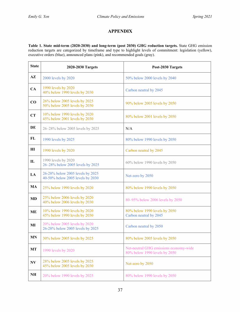
Emily G. Yen Climate Policy and Emissions Spring 2021
37
APPENDIX
Table 1. State mid-term (2020-2030) and long-term (post 2030) GHG reduction targets. State GHG emission reduction targets are categorized by timeframe and type to highlight levels of commitment: legislation (yellow), executive orders (blue), announced plans (pink), and recommended goals (gray).
State 2020-2030 Targets Post-2030 Targets
AZ 2000 levels by 2020 50% below 2000 levels by 2040
CA 1990 levels by 2020 40% below 1990 levels by 2030 Carbon neutral by 2045
CO 26% below 2005 levels by 2025 50% below 2005 levels by 2030 90% below 2005 levels by 2050
CT 10% below 1990 levels by 2020 45% below 2001 levels by 2030 80% below 2001 levels by 2050
DE 26–28% below 2005 levels by 2025 N/A
FL 1990 levels by 2025 80% below 1990 levels by 2050
HI 1990 levels by 2020 Carbon neutral by 2045
IL 1990 levels by 2020 26–28% below 2005 levels by 2025 60% below 1990 levels by 2050
LA 26-28% below 2005 levels by 2025 40-50% below 2005 levels by 2030 Net-zero by 2050
MA 25% below 1990 levels by 2020 80% below 1990 levels by 2050
MD 25% below 2006 levels by 2020 40% below 2006 levels by 2030 80–95% below 2006 levels by 2050
ME 10% below 1990 levels by 2020 45% below 1990 levels by 2030
80% below 1990 levels by 2050 Carbon neutral by 2045
MI 20% below 2005 levels by 2020 26-28% below 2005 levels by 2025 Carbon neutral by 2050
MN 30% below 2005 levels by 2025 80% below 2005 levels by 2050
MT 1990 levels by 2020 Net-neutral GHG emissions economy-wide 80% below 1990 levels by 2050
NV 28% below 2005 levels by 2025 45% below 2005 levels by 2030 Net-zero by 2050
NH 20% below 1990 levels by 2025 80% below 1990 levels by 2050
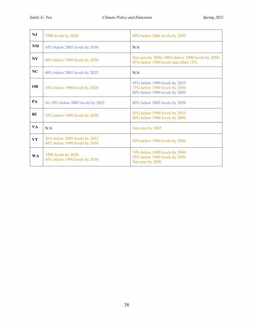
Emily G. Yen Climate Policy and Emissions Spring 2021
38
NJ 1990 levels by 2020 80% below 2006 levels by 2050
NM 45% below 2005 levels by 2030 N/A
NY 40% below 1990 levels by 2030 Net-zero by 2050; 100% below 1990 levels by 2050: 85% below 1990 levels and offset 15%
NC 40% below 2005 levels by 2025 N/A
OR 10% below 1990 levels by 2020 45% below 1990 levels by 2035 75% below 1990 levels by 2050 80% below 1990 levels by 2050
PA 26–28% below 2005 levels by 2025 80% below 2005 levels by 2050
RI 10% below 1990 levels by 2020 45% below 1990 levels by 2035 80% below 1990 levels by 2050
VA N/A Net-zero by 2045
VT 26% below 2005 levels by 2025 40% below 1990 levels by 2030 80% below 1990 levels by 2050
WA 1990 levels by 2020 45% below 1990 levels by 2030
70% below 1990 levels by 2040 95% below 1990 levels by 2050 Net-zero by 2050
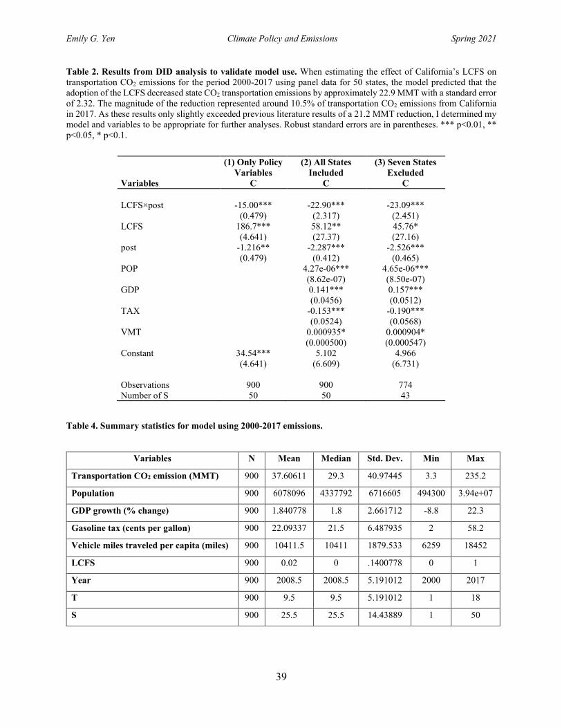
Emily G. Yen Climate Policy and Emissions Spring 2021
39
Table 2. Results from DID analysis to validate model use. When estimating the effect of California’s LCFS on transportation CO2 emissions for the period 2000-2017 using panel data for 50 states, the model predicted that the adoption of the LCFS decreased state CO2 transportation emissions by approximately 22.9 MMT with a standard error of 2.32. The magnitude of the reduction represented around 10.5% of transportation CO2 emissions from California in 2017. As these results only slightly exceeded previous literature results of a 21.2 MMT reduction, I determined my model and variables to be appropriate for further analyses. Robust standard errors are in parentheses. *** p<0.01, ** p<0.05, * p<0.1.
(1) Only Policy Variables
(2) All States Included
(3) Seven States Excluded
Variables C C C LCFS×post -15.00*** -22.90*** -23.09*** (0.479) (2.317) (2.451) LCFS 186.7*** 58.12** 45.76* (4.641) (27.37) (27.16) post -1.216** -2.287*** -2.526*** (0.479) (0.412) (0.465) POP 4.27e-06*** 4.65e-06*** (8.62e-07) (8.50e-07) GDP 0.141*** 0.157*** (0.0456) (0.0512) TAX -0.153*** -0.190*** (0.0524) (0.0568) VMT 0.000935* 0.000904* (0.000500) (0.000547) Constant 34.54*** 5.102 4.966 (4.641) (6.609) (6.731) Observations 900 900 774 Number of S 50 50 43
Table 4. Summary statistics for model using 2000-2017 emissions.
Variables N Mean Median Std. Dev. Min Max
Transportation CO2 emission (MMT) 900 37.60611 29.3 40.97445 3.3 235.2
Population 900 6078096 4337792 6716605 494300 3.94e+07
GDP growth (% change) 900 1.840778 1.8 2.661712 -8.8 22.3
Gasoline tax (cents per gallon) 900 22.09337 21.5 6.487935 2 58.2
Vehicle miles traveled per capita (miles) 900 10411.5 10411 1879.533 6259 18452
LCFS 900 0.02 0 .1400778 0 1
Year 900 2008.5 2008.5 5.191012 2000 2017
T 900 9.5 9.5 5.191012 1 18
S 900 25.5 25.5 14.43889 1 50
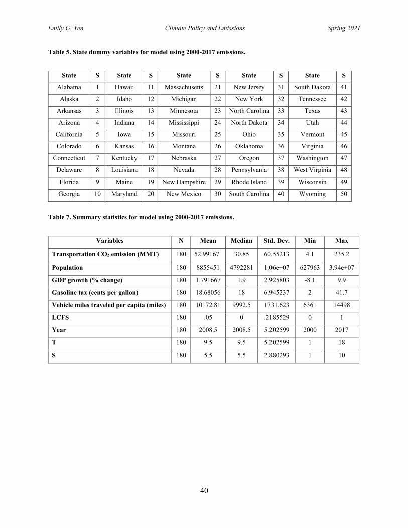
Emily G. Yen Climate Policy and Emissions Spring 2021
40
Table 5. State dummy variables for model using 2000-2017 emissions.
State S State S State S State S State S
Alabama 1 Hawaii 11 Massachusetts 21 New Jersey 31 South Dakota 41
Alaska 2 Idaho 12 Michigan 22 New York 32 Tennessee 42
Arkansas 3 Illinois 13 Minnesota 23 North Carolina 33 Texas 43
Arizona 4 Indiana 14 Mississippi 24 North Dakota 34 Utah 44
California 5 Iowa 15 Missouri 25 Ohio 35 Vermont 45
Colorado 6 Kansas 16 Montana 26 Oklahoma 36 Virginia 46
Connecticut 7 Kentucky 17 Nebraska 27 Oregon 37 Washington 47
Delaware 8 Louisiana 18 Nevada 28 Pennsylvania 38 West Virginia 48
Florida 9 Maine 19 New Hampshire 29 Rhode Island 39 Wisconsin 49
Georgia 10 Maryland 20 New Mexico 30 South Carolina 40 Wyoming 50
Table 7. Summary statistics for model using 2000-2017 emissions.
Variables N Mean Median Std. Dev. Min Max
Transportation CO2 emission (MMT) 180 52.99167 30.85 60.55213 4.1 235.2
Population 180 8855451 4792281 1.06e+07 627963 3.94e+07
GDP growth (% change) 180 1.791667 1.9 2.925803 -8.1 9.9
Gasoline tax (cents per gallon) 180 18.68056 18 6.945237 2 41.7
Vehicle miles traveled per capita (miles) 180 10172.81 9992.5 1731.623 6361 14498
LCFS 180 .05 0 .2185529 0 1
Year 180 2008.5 2008.5 5.202599 2000 2017
T 180 9.5 9.5 5.202599 1 18
S 180 5.5 5.5 2.880293 1 10
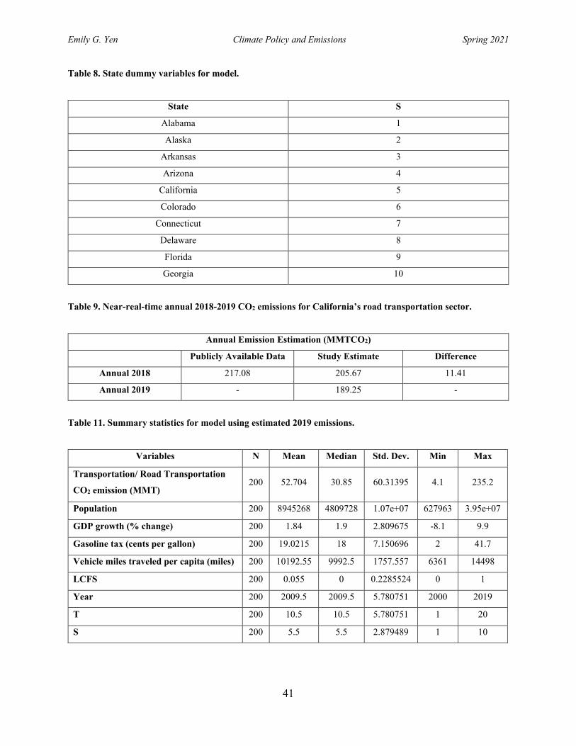
Emily G. Yen Climate Policy and Emissions Spring 2021
41
Table 8. State dummy variables for model.
State S
Alabama 1
Alaska 2
Arkansas 3
Arizona 4
California 5
Colorado 6
Connecticut 7
Delaware 8
Florida 9
Georgia 10
Table 9. Near-real-time annual 2018-2019 CO2 emissions for California’s road transportation sector.
Annual Emission Estimation (MMTCO2)
Publicly Available Data Study Estimate Difference
Annual 2018 217.08 205.67 11.41
Annual 2019 - 189.25 -
Table 11. Summary statistics for model using estimated 2019 emissions.
Variables N Mean Median Std. Dev. Min Max
Transportation/ Road Transportation
CO2 emission (MMT) 200 52.704 30.85 60.31395 4.1 235.2
Population 200 8945268 4809728 1.07e+07 627963 3.95e+07
GDP growth (% change) 200 1.84 1.9 2.809675 -8.1 9.9
Gasoline tax (cents per gallon) 200 19.0215 18 7.150696 2 41.7
Vehicle miles traveled per capita (miles) 200 10192.55 9992.5 1757.557 6361 14498
LCFS 200 0.055 0 0.2285524 0 1
Year 200 2009.5 2009.5 5.780751 2000 2019
T 200 10.5 10.5 5.780751 1 20
S 200 5.5 5.5 2.879489 1 10