Assessing and Improving Neural Network Predictions by the Bootstrap Algorithm

Gerhard Paass German National Research Center for Computer Science (GMD)

D-5205 Sankt Augustin, Germany e-mail: paass<Dgmd.de

Abstract

The bootstrap algorithm is a computational intensive procedure to derive nonparametric confidence intervals of statistical estimators in situations where an analytic solution is intractable. It is ap­plied to neural networks to estimate the predictive distribution for unseen inputs. The consistency of different bootstrap procedures and their convergence speed is discussed. A small scale simulation experiment shows the applicability of the bootstrap to practical problems and its potential use.

1 INTRODUCTION

Bootstrapping is a strategy for estimating standard errors and confidence intervals for parameters when the form of the underlying distribution is unknown. It is particularly valuable when the parameter of interest is a complicated functional of the true distribution. The key idea first promoted by Efron (1979) is that the relationship between the true cumulative distribution function (cdf) F and the sample of size n is similar to the relationship between the empirical cdf Fn and a secondary sample drawn from it. So one uses the primary sample to form an estimate Fn and calculates the sampling distribution of the parameter estimate under Fn. This calculation is done by drawing many secondary samples and finding the estimate, or function of the estimate, for each. If:Fn is a good approximation of F, then H n , the sampling distribution of the estimate under Fn , is a generally good approximation to the sampling distribution for the estimate under F. H n is

196

Assessing and Improving Neural Network Predictions by the Bootstrap Algorithm 197

called the bootstrap distribution of the parameter. Introductory articles are Efron and Gong (1983) and Efron and Tibshirani (1986). For a survey of bootstrap results see Hinkley (1988) and DiCiccio and Romano (1988).

A neural networks often may be considered as a nonlinear or nonparametric regres­sion model

Z = g/3(Y) + € (1)

which d~fines the relation between the vectors Y and z of input and output variables. The ter:n € can be interpreted as a random 'error' and the function g/3 depends on some Ul_kown parameter f3 which may have infinite dimension. Usually the network is used to determine a prediction Zo = g/3(Yo) for some new input vector Yo. If the data is a random sample, an estimate P differs from the true value of f3 because of the sampling error and consequently the prediction g~(yo) is different from the true prediction. In this paper the bootstrap approach is used to approximate a sampling distribution of the prediction (or a function thereof) and to estimate parameters of that distribution like its mean value, variance, percentiles, etc. Bootstrapping procedures are closely related to other resampling methods like cross validation and jackknife (Efron 1982). The jackknife can be considered as a linear approximation to the bootstrap (Efron, Tibshirani 1986).

In the next section different versions of the bootstrap procedure for feedforward neural networks are defined and their theoretical properties are reviewed. Main points are the convergence of the bootstrap distribution to true theoretical distri­bution and the speed of that convergence. In the following section the results of a simulation experiment for a simple backprop model are reported and the applica­tion of the bootstrap to model selection is discussed. The final section gives a short summary.

2 CONSISTENCY OF THE BOOTSTRAP FOR FEEDFORWARD NEURAL NETWORKS

Assume X (n) := (Xl, ... , xn) is the available independent, identically distributed (iid) sample from an underlying cdf F where Xi = (Zi' Yi) and Fn is the correspond­ing empirical cdf. For a given Yo let T} = T}(g/3(Yo)) be a parameter of interest of the prediction, e.g. the mean value of the prediction of a component of Z for Yo.

The pairwise bootstrap algorithm is an intuitive way to apply the bootstrap notion to regression. It was proposed by Efron (1982) and involves the independent repetition of following steps for b = 1, ... , B.

1. A sample XbCn) of size n is generated from Fn. Notice that this amounts to the random selection of n elements from X(n) with replacement.

2. An estimate TJb is determined from X;(n).

The resulting empirical cdf of the TJb, b = 1, ... ,n is denoted by H B and approxi­mates the sampling distribution for the estimate TJ under Fn. The standard devia­tion of HE is an estimate of the standard error of T}(Fn) , and [Hnl(a), Hn 1(1- a)] is an approximate (1 - 2a) central confidence interval.

198 Paass

In general two conditions are necessary for the bootstrap to be consistent:

• The estimator, e.g. fib has to be consistent .

• The functional which maps F to HB has to be smooth.

This requirement can be formalized by a uniform weak convergence condition (Di­Ciccio, Romano 1988). Using these concepts Freedman (1981) proved that for the parameters of a linear regression model the pairwise bootstrap procedure is con­sistent, i.e. yields the desired limit distribution for n, B --+ 00. Mammen (1991) showed that this also holds for the preuictive distribution of a linear model (i.e. linear contrasts). These results hold even if the errors are heteroscedastic, i.e. if the distribution of fi depends on the value of Yi.

The performance of the bootstrap for linear regression is extensively discussed by Wu (1986). It turns out that the small sample properties can be different from the asymptotic relations and the bootstrap may exhibit a sizeable bias. Various procedures of bias correction have been proposed (DiCiccio, Romano 1988). Beran (1990) discusses a calibrated bootstrap prediction region containing the prediction g,6(YO)+f with prescribed probability a. It requires a sequence of nested bootstraps. Its coverage probability tends to a at a rate up to n-2 • Note that this procedure can be applied to nonlinear regression models (1) with homoscedastic errors (Example 3 in Beran (1990, p.718) can be extended to this case).

Biases especially arise if the errors are heteroscedastic. Hinkley (1988) discusses the parametric modelling of dependency of the error distribution (or its variance) from Y and the application of the bootstrap algorithm using this model. The problem is here to determine this parametric dependency from the data. As an alternative Wu (1986) and Liu (1988) take into account heteroscedasticity in a nonparametric way. They propose the following wild bootstrap algorithm which starts with a consistent estimate /3 based on the sample X(n). Then the set of residuals (i l , ... ,in) with fi := Zi - g~(yd is determined. The approach attempts to mimic the conditional

distribution of Z given Yi in a very crude way by defining a distribution Oi whose first three moments coincide with the observed residual fi:

J udOj(u) = 0 J u2 dOi (u) = f; J u3dOi (u) = f~ (2)

Two point distributions are used which are uniquely defined by this requirement (Mammen 1991, p.121). Then the following steps are repeated for b = 1, ... , B:

1. Independently generate residuals fi according to Oi and generate observa­tions z; := 9p(Yi) + fi for i = (1, ... , n). This yields a new sample X;(n) of size n.

2. An estimate fit is determined from Xb(n).

The resulting empirical cdf of the fit is then taken as the bootstrap distribution H B which approximates the sampling distribution for the estimate fI under Fn. Mammen (1991, p.123) shows that this algorithm is consistent for the prediction of linear regression models if the least square estimator or M-estimators are used and discusses the convergence speed of the procedure.

Assessing and Improving Neural Network Predictions by the Bootstrap Algorithm 199

The bootstrap may also be applied to nonparameric regression models like kernel­type estimators of the form

g(y) = [g?~:~~(~lJ (3)

with kernel [{ and bandwidth h. These models are related to radial basis functions discussed in the neural network literature. For those models the pairwise bootstrap does not work (HardIe, Mammen 1990) as the algorithm is not forced to perform locall:J., ~raging. To account for heteroscedasticity in the errors of (1) HardIe (1990, p.103) advocates the use of the wild bootstrap algorithm described above. Under some regularity conditions he shows the convergence of the bootstrap distribution of the kernel estimator to the correct limit distribution.

To summarize the bootstrap often is used simply because an analytic derivation of the desired sampling distribution is too complicated. The asymptotic investigations offer two additional reasons:

• There exist versions of the bootstrap algorithm that have a better rate of convergence than the usual asymptotic normal approximation. This effect has been extensively discussed in literature e.g. by Hall (1988), Beran (1988), DiCiccio and Romano (1988, p.349), Mammen (1991, p.74).

• There are cases where the bootstrap works, even if the normal approxima­tion breaks down. Bickel and Freedman (1983) for instance show, that the bootstrap is valid for linear regression models in the presence of outliers and if the number of parameters changes with n. Their results are discussed and extended by Mammen (1991, p.88ff).

3 SIMULATION EXPERIMENTS

To demonstrate the performance of the bootstrap for real real problems we inves­tigated a small neural network. To get a nonlinear situation we chose a "noisy" version of the xor model with eight input units YI, ... ,Ys and a single output unit z. The input variables may take the values 0 and 1. The output unit of the true model is stochastic. It takes the values 0.1 and 0.9 with the following probabilities:

p(y = 0.9) = 0.9 if Xl + X2 + X3 + X4 < 3 and X5 + X6 + X7 + Xs < 3 p(y = 0.9) = 0.1 if Xl + X2 + X3 + X4 < 3 and X5 + X6 + X7 + Xs > 3 p(y = 0.9) = 0.1 if Xl + X2 + X3 + X4 > 3 and X5 + X6 + X7 + XS < 3 p(y = 0.9) = 0.9 if Xl + X2 + X3 + X4 > 3 and X5 + X6 + X7 + Xs > 3

In contrast to the simple xor model generalization is possible in this setup. We generated a training set X( n) of n = 100 inputs using the true model.

We used the pairwise bootstrap procedure described above and generated B = 30 different bootstrap samples X;(n) by random selection from X(n) with replace­ment. This number of bootstrap samples is rather low and only will yield reliable information on the central tendency of the prediction. More sensitive parameters of

200 Paass

Input vectors

Y1 Yg

10110110

01110110

1 1 1 101 1 0

00001110

10001110

01001110

11001110

00101110

10101110

01101110

1 1 101 1 1 0

00011110

10011110

01011110

11011110

00111110

... true expected value

Bootstrap Distribution of Prediction

0.0 0.5

t---------tl ~ H r------mJ-;

...---------.,14 I~

....

.A l!:rt A.. I· ~

zill

t------::zs:~~

.A I!H l{l}-i

~

.A value predicted by the original backprop model

~------f--llnH percentiles of the

10 25 50 75 90 bootstrap distribution

1.0

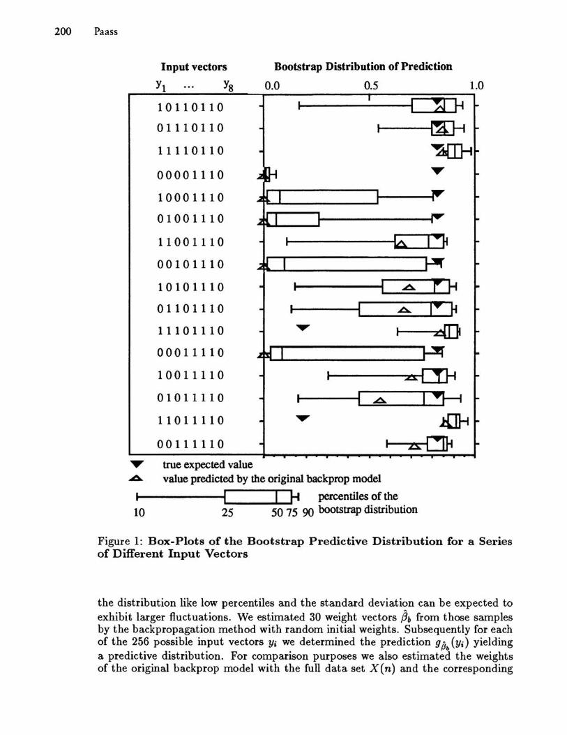
Figure 1: Box-Plots of the Bootstrap Predictive Distribution for a Series of Different Input Vectors

the distribution like low percentiles and the standard deviation can be expected to exhibit larger fluctuations. We estimated 30 weight vectors ~b from those samples by the backpropagation method with random initial weights. Subsequently for each of the 256 possible input vectors Yi we determined the prediction g~1> (Yi) yielding a predictive distribution. For comparison purposes we also estimated the weights of the original backprop model with the full data set X (n) and the corresponding

Assessing and Improving Neural Network Predictions by the Bootstrap Algorithm 201

Table 1: Mean Square Deviation from the True Prediction

INPUT HIDDEN MEAN SQUARE DIFFERENCE TYPE UNITS BOOTSTRAP DB FULL DATA DF

training 2 0.18 0.19 inputs 3 0.17 0.19

4 0.17 0.19

ne I-training 2 0.30 0.34 inputs 3 0.35 0.38

4 0.37 0.42

Table 2: Coverage Probabilities of the Bootstrap Confidence Interval for Prediction

HIDDEN UNITS

2 3 4

predictions.

FRACTION OF CASES WITH TRUE PREDICTION IN [q2S, q7S] [q10, qgo]

0.47 0.44 0.43

0.77 0.70 0.70

For some of those input vectors the results are shown in figure 1. The distributions differ greatly in size and form for the different input vectors. Usually the spread of the predictive distribution is large if the median prediction differs substantially from the true value. This reflects the situation that the observed data does not have much information on the specific input vector. Simply by inspecting the predictive distribution the reliability of a predictions may be assessed in a heuristic way. This may be a great help in practical applications.

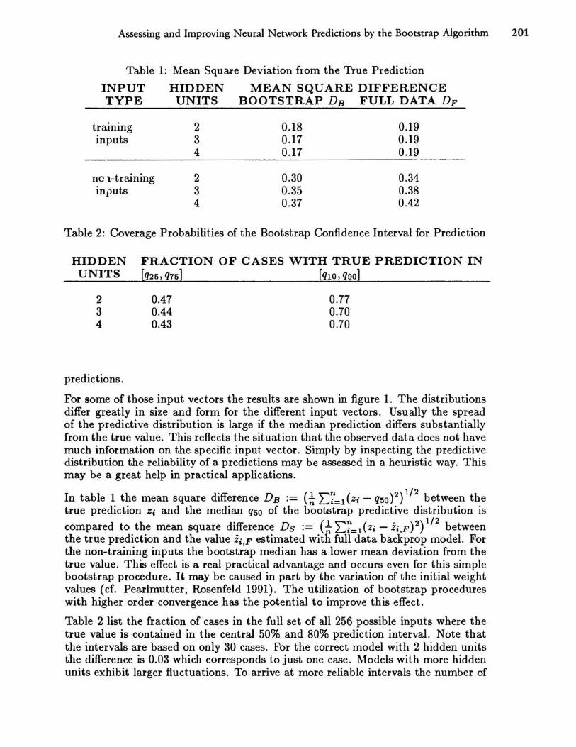
In table 1 the mean square difference DB := (~L:~=1 (Zi - qSo)2) 1/2 between the true prediction Zi and the median qso of the bootstrap predictive distribution is compared to the mean square difference Ds := (1. L:?=l(Zi - Zi,F)2)1/2 between the true prediction and the value Zi,F estimated with full data backprop model. For the non-training inputs the bootstrap median has a lower mean deviation from the true value. This effect is a real practical advantage and occurs even for this simple bootstrap procedure. It may be caused in part by the variation of the initial weight values (cf. Pearlmutter, Rosenfeld 1991). The utilization of bootstrap procedures with higher order convergence has the potential to improve this effect.

Table 2 list the fraction of cases in the full set of all 256 possible inputs where the true value is contained in the central 50% and 80% prediction interval. Note that the intervals are based on only 30 cases. For the correct model with 2 hidden units the difference is 0.03 which corresponds to just one case. Models with more hidden units exhibit larger fluctuations. To arrive at more reliable intervals the number of

202 Paass

HIDDEN UNITS

2 3 4

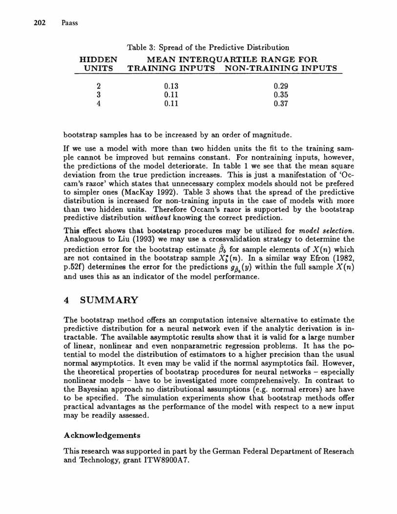
Table 3: Spread of the Predictive Distribution

MEAN INTERQUARTILE RANGE FOR TRAINING INPUTS NON-TRAINING INPUTS

0.13 0.11 0.11

0.29 0.35 0.37

bootstrap samples has to be increased by an order of magnitude.

If we use a model with more than two hidden units the fit to the training sam­ple cannot be improved but remains constant. For nontraining inputs, however, the predictions of the model deteriorate. In table 1 we see that the mean square deviation from the true prediction increases. This is just a manifestation of 'Oc­cam's razor' which states that unnecessary complex models should not be prefered to simpler ones (MacKay 1992). Table 3 shows that the spread of the predictive distribution is increased for non-training inputs in the case of models with more than two hidden units. Therefore Occam's razor is supported by the bootstrap predictive distribution without knowing the correct prediction.

This effect shows that bootstrap procedures may be utilized for model selection. Analoguous to Liu (1993) we may use a crossvalidation strategy to determine the prediction error for the bootstrap estimate ~b for sample elements of X (n) which are not contained in the bootstrap sample X; (n). In a similar way Efron (1982, p.52f) determines the error for the predictions g~b(Y) within the full sample X(n) and uses this as an indicator of the model performance.

4 SUMMARY

The bootstrap method offers an computation intensive alternative to estimate the predictive distribution for a neural network even if the analytic derivation is in­tractable. The available asymptotic results show that it is valid for a large number of linear, nonlinear and even nonparametric regression problems. It has the po­tential to model the distribution of estimators to a higher precision than the usual normal asymptotics. It even may be valid if the normal asymptotics fail. However, the theoretical properties of bootstrap procedures for neural networks - especially nonlinear models - have to be investigated more comprehensively. In contrast to the Bayesian approach no distributional assumptions (e.g. normal errors) are have to be specified. The simulation experiments show that bootstrap methods offer practical advantages as the performance of the model with respect to a new input may be readily assessed.

Acknowledgements

This research was supported in part by the German Federal Department of Reserach and Technology, grant ITW8900A 7.

Assessing and Improving Neural Network Predictions by the Bootstrap Algorithm 203

References Beran, R. (1988): Prepivoting Test Statistics: A Bootstrap View of Asymptotic Refinements. Journal of the American Statistical Association. vol. 83, pp.687-697. Beran, R. (1990): Calibrating Prediction Regions. Journal of the American Statis­tical Association., vol. 85, pp.715-723. Bickel, P.J., Freedman, D.H. (1981): Some Asymptotic Theory for the Bootstrap. The Annals of Statistics, vol. 9, pp.1l96-1217. Bickel, P.J., Freedman, D.H. (1983): Bootstrapping Regression Models with many Parame~ers. In P. Bickel, K. Doksum, J .C. Hodges (eds.) A Festschrift for Erich Lehmann. Wadsworth, Belmont, CA, pp.28-48. DiCiccio, T.J., Romano, J.P. (1988): A Review of Bootstrap Confidence Intervals. J. Royal Statistical Soc., Ser. B, vol. 50, pp.338-354. Efron, B. (1979): Bootstrap Methods: Another Look at the Jackknife. The Annals of Statistics, vol 7, pp.1-26. Efron, B. (1982): The Jackknife, the Bootstrap and Other Resampling Plans. SIAM, Philadelphia. Efron, B., Gong, G. (1983): A leisure look at the bootstrap, the jackknife and crossvalidation. A merican Statistician, vol. 37, pp.36-48. Efron, B., Tibshirani (1986): Bootstrap methods for Standard Errors, Confidence Intervals, and other Measures of Statistical Accuracy . Statistical Science, vol 1, pp.54-77. Freedman, D.H. (1981): Bootstrapping Regression Models. The Annals of Statis­tics, vol 9, p.1218-1228. HardIe, W.(1990): Applied Nonparametric Regression. Cambridge University Press, Cambridge. HardIe, W., Mammen, E. (1990): Bootstrap Methods in Nonparametric Regression. Preprint Nr. 593. Sonderforschungsbereich 123, University of Heidelberg. Hall, P. (1988): Theoretical Comparison of Bootstrap Confidence Intervals. The Annals of Statistics, vol 16, pp.927-985. Hinkley, D .. (1988): Bootstrap Methods. Journal of the Royal Statistical Society, Ser. B, vol.50, pp.321-337. Liu, R. (1988): Bootstrap Procedures under some non i.i.d. Models. The Annals of Statistics, vo1.16, pp. 1696-1708. Liu, Y. (1993): Neural Network Model Selection Using Asymptotic Jackknife Esti­mator and Cross-Validation Method. This volume. MacKay, D. J. C. (1992): Bayesian Model Comparison and Backprop Nets. In Moody, J .E., Hanson, S.J., Lippman, R.P. (eds.) Advances in Neural Information Processing Systems 4. Morgan Kaufmann, San Mateo, pp.839-846. Mammen, E. (1991): When does Bootstrap Work: Asymptotic Results and Simu­lations. Preprint Nr. 623. Sonderforschungsbereich 123, University of Heidelberg. Pearlmutter, B.A., Rosenfeld, R. (1991): Chaitin-Kolmogorov Complexity and Gen­eralization in Neural Networks. in Lippmann et al. (eds.): Advances in Neural Information Processing Systems 3, Morgan Kaufmann, pp.925-931. C.F.J. Wu (1986): Jackknife, Bootstrap and other Resampling Methods in Regres­sion Analysis. The Annals of Statistics, vol. 14, p.1261-1295.