Embed Size (px)
Citation preview
NASA CR-134538
ASSEMBLY AND ANALYSISFRAGMENTATION DATA FOR
PROPELLANT VESSELS
OFLIQUID
• E. Bake , V B Parr, R L Bessey, and P. A. Cox
By W r ....SOUTHWEST RESEARCH INSTITU
son nonoTxo_r._or._,or _*, '_L_I
NATIONAL AERONAUTICS AND SPACE ADMI_TIONLEWIS RESEARCH CENTER
AEROSPACE SAFETY RESEARCH AND DATA INSTITUTE
CLEVELAND, OHIO 44135
C. David Miller, Project Manager
R. D. Siewert, Project Manager
Contract NAS 3-16009
(NI_A-C&-134536) ASSeMbLY AND ANALYSISOF FEAGME_IA_ICN EALA EG_ LI_UIp
kRCEELLANr ¥EFS_LS (Southwest i_edrch
rn_t.) 236 _ HC $1_.00 CSCL 20K
GJ/J2
N7q-15o25
FOREWORD
.d.:
7'
4
%
Many staff members at Southwest Research Institute c_ntributed
substantially to the multifaceted effort required during the work reported
here. The authors gratefully acknowledge _he special technical cont_'ibut_ons
of the following:
o Mr. A. B. Wenzel, for many of the initial visits and contacts
to _,ather data, for review of Project PYRO films, and for
assistance in project management.
o Mr. M. A. Sissung, for review of Project PYRO films,
assistance in literature surveys, and report editim,..
o Mr. R. Blackstone, for assistance in statistical _tudies.
In addition, these individuals helped the authors substantially in ente fine
data into the ASRDI data bank by reviewing documents and fillin_ out ASRDI
Forms 102A for these dncuments.
The technica! support o_ personnel at both NASA-Lewis Research
Center and NASA-Kennedy Space Cen_er contributed materially to the succes_
of this work. In particular, Mr. C. David Miller at NASA-Lewis provided
excellent technical guidance throuahout the project, and Mr. Jamc._ H. Deese
at NASA-Kennedy gave us much insight into blast effects of liquid propellant
explosions and provtded us with tht three most comp!ete fraament maps trom
such explosions.
I'R!.C,2)I),G PAGE B' ', .................. ...... ,.L i" .......
iii

TABLE OF CONTENTS
Pa_e
LIST OF FIGURESvii
LIST OF TABI,ES
SUMMAt_ Y
INTRODUCTION
B ack ground
Related Work
Purpose of Present Work
Scope of Present Work
Significance
N 1_
xii
1
1
3
6
6
6
I°RETRIEVAL OF FRAGMENTATION DATA FOR
LIQUID PROPELLANT VESSELS
II. DETERMINATION OF BLAST YIELD13
A°
B.
C.
D.
General
Project PYRO and Related Experiments
Work of Farber and Deese
Estimation of Blast Wave Properties
15
2O
26
Ill. DETERMINATION OF FRAGMENT VELOCITY
DISTRIBUTION.t<i
Ao
B.
C.
D.
E_e
General
Reduction of Film Data
Methoas of Predicting Velocity
Correlation of Velocity Prediction
Methods with Data
Frequency Distribution of Initial
Velocity
4q
-t q
67
o 7
IVoDETERMINATION OF FPAGMfZNT SIZE AND RANGE
104
Ao
B °
C.
D.
°
Retrieval of Data from Accidot.ts and
Tests
Data tted,_ction
Stati:_tical Studies
Methods of Prediction of Range Versus
gra':nent and Blast Yield Parameters
Correlation
IO-t
106
106
11-t
IZ9
P_ ;er'rmt, ,_
-"'.-,,,n.';tj PAGP, BI,AVV ':¢;7" l'II _ I)

Table of Contents (Cont'd) -
V° EFFECTS OF FRAGMENTS
f.
B.
C °
Introduction
The Probability of Arrival of a Fragment
of Specified Characteristics Versus Range
Vulne rab ility C rite r ia
VI. DISCUSSION OF RESULTS
VII. C ONC LUo.ONS
VIII. R_:C OMME NDATIONS
APPENDICES
APPENDIX A - Model Analysis for Mixing of Liquid
Rocket Propellants
APPENDIX B - Summary of Data Obtained From Films
Read
APPENDIX C - Model Analyses for Fragment Velocities,
Range, Etc., for Bursting Liquid Pro-
pellant Vessels
APPENDIX I) - Computer Pro, gram Entitled /WZ/ In
Fort :an IV
APPENDIX E - Computer Program Entitled /ROOT/
In Fortran IV
APPENDIX F - Calculation of "W" Goodness of Fit
Statistic from Reference 36
APPENDIX G - Calculation (_t' Approximate Probab:lity
for Obtaiping the Calc 'lated V,:due td "W"
APPENDIX ti - Coml)_lter ProR ram E,_titlvd /TEMP/ It,
Fortran IV
APPENDIX I List of Symbols
REFE RENCES
Page
135
135
136
139
142.
146
148
150
165
175
186
19 a
ZOO
207
200
vi
%
<
H
No.
4
5
6
7
q
I0
11
12
1-;
1-3
16
17
LIS_I OF FIGUREC
Title
Normalized Pressure and Impulse Yields from Explusion _,5
NzO4/Aerozine 50
Representatlve Shock Impulses Sho_ving Coalescence of Shock
Waves from Dissimilar Sources (Stages (a) through (d} }
Maximum Enerov Release for a Three-Component LiqL1id
Propei]ant Mixture (Ref. gT)
Mixing Function or Spill Function for Thrce-Con_ponent
Liquid Propellant Spill Tests (Ref. 27)
Yield Potential as Time Function (Ref. ZT)
Actual Yield for Random Ignition and Detonation (Ref. Z7)
Estimated Explosive Yield as a Function of Propellant
Weight (Ref. 17)
Terrninal Vield vs. Impact Velocity for Hypergolic High-
Velocity Impact (Ref. 16)
Pressure vs. Scaled Distance for Hypergolic Tests
Scaled Positive Impulse vs. Scaled Distance for }Iyper-
golic Tests
I,,nition Time vs. Yield LOz/RP-1 CBM
Pres.q_lre vs. Scaled Distance for LOt/lIP-1 CBM Case
Scaled Positive Impulse vs. Scaled Distance for LO2/RP-I
CBM Case
I_:nition rime v3. Normalized Yield LO2/RP-1 CBGS
Pressure vs. Scaled Distar_ce far I Oz/RP- 1 CBGS-V Case
Scaled Positive Impulse "¢s. Scaled Distance for LOg/RP- 1
CBGS-V Case
Termi_,al Yield vs. Impact Velocity for LOz/RP-I {}_ef. 16)
vii
I-D[ _ t'
I
16
21
23
24
2%
Z7
0
3Z
3-t
3_
36
37
38
_Q
-t 1

List of Figures (Cont'd) -
No. Title
18 Ignition Time vs.
19
Z0
ZI
Z2
23
Z4
25
26
27
28
29
3O
51
32
_3
34
Yield LOz/LH z CBM
"Pressure vs. Scaled Distance for LOz/LH z CBM Case
Scaled Positive impulse vs. Scaled Distance for LOz/
LH Z CBM Case
Ignition Time vs. Normalized Yield LO2/LH 2 CBGS
Pressure vs. Scaled Distance for LOz/LH Z CBGS-V Case
Scaled Positive Impulse vs. Scaled Distance fo_ LOz/LH Z
CBGS- V Case
Ter_ninal Yield vs. Impact Velocity for LOz/IH Z (Ref. 16)
Plan View of Camera Locations During PYRC) Tests
Fireball and Fragment as Viewed by a Canlera Located
at Position A
Scht:h_t.ti, <h,_wi,,r Actu.tl and Calculated _/ragment
Ve rtic al [)l_ },ldccments
Geometry for Fragment Position for Duplicate Views
Ma_xirnum Fraument Velocity as a Function of Number of
F'r a_me nts
Maximum Fracment Velocity vs. Mass R_tio
Comparison of Taylor-Price to SwRI Solutions for
Adiabatic Case
Schernati " for Acceleration of Appurtenances by Propellant
Blast
Inter:_ction of Blast Wave with Irregular Object
Time History of Net Transverse P:essure on Object
During Passage of a Blast Wave
42
43
44
45
46
47
48
50
54
%6
5o
73
74
76
77
79
8O
viii
i
_ P
i
I
.
List of Figures (Cont'd) -
No.
35
36
37
38
39
Title
Blast Wave Time Constant b vs. Dimensionless Over-
pressure P
Fragment Velocity: Correlation of Data from PYRO
LHz/LO Z Tests with Tbeoretical Values, W t = ZOO ib
Fragment Velocity: Correlation of Data from PYRO
Tests with Theoretical Values, W t = 1000 Ib
Fragment Velocity as a Function of Sound Speed in the
Explosive Products
Initial Velocity Distribution, CBM, LOz/L {Z, Log Normal
I_o _ S
4O
41
42
43
44
.'B
40
.t7
.',4
Irltial Velocity Distribution, CBM, LO_/RP-I, Log
Normal Plots
Inltial Velocity Distribution, CBGS, LOz/LH Z, Log
Normal l_ots
Initia] Velocity Distribution, GBGS, LOz/RP-I, Log
Normal Plots
Event 3 Probability Distributio_ (Normal), Distance
Event 3 Probability Distribution (Log Normal),
Event I Probability Distribution (Log Normal),
Area A
Ev_.ut 4 Probabilit) Distribution (Log Normal} Weight W
Event I Probability Distribtltion (NornTal), Area/Weight
{AIW)
.\pproxinaate Probability Percet:tage Points of "W" Test
f{}r Normality (n = c}}
R
Di stance R
Projected
NIean I)i_tancc vs. Yield
-0 ,Me.,n [}ist:,nc{' vs. Yield in lb TNT
ix
81
87
88
93
i00
I00
lO1
101
112
113
118
119
1gO
1"1
112

i
L
List of F_gures (Cont'd) -
No. Title
51
52
53
54
Mean Distance vs. Yield, with Estimated Range Containing
95% of the Fragments (Ros)
Standard Deviation S vs. Mean Distance' R
Geometric Mean (A/W) vs. Geometric Mean Distance
Regression of Geometric Mean (A/W 2/3) vs. Geometric
Me an Range
X
lZ6
130
131
132

No.
II
III
IV
V
VI
VII
VIII
IX
X
XI
XII
XIII
XIV
XV
XVI
XVII
XVIII
XIX
LIST OF TABLES
T itle
Summary of Agencies Visited to Obtain Fragmentation
Data or Documents
Detonation Energy Gquivalents for Selected Liquid
Propellants
Predicted Ma):imum Blast Yields (Ref. 241
Estimates of Terminal Yield (Ref. 16)
Summary of Fragment Velocity Meas,lrement_
Comparison of Predicted Fragments with Pittrnan's Data
(Ref. 33)
Drag Coefficients C D, of Various Shapes {Source: Ref. 35)
Fragment Velocity Predictions Corer
Grouping of Tests by Propellant and
-ed with Measurements
,nfiguration
Percentiles, Means and Standard Deviatiol,_: for Grouped
Velocity Data (fps)
Chart of Events
Calculated Statistics for Parameters of Eight Exe,,,ts
Percentiles for Plotting Parameters of Events 1 Thro_Igh 8
Summary of Fragment Data
Approximate Percentage Points of "W" Test for Normality
(u = 9}
mary of "W" Test for Normality for R, W, A, (A/W)
Confidence Limits on Mean, Standard Deviation and Distance
Containing 95% of Fragments
Predicted vs. Measured Fragment Ranges
Constants for Vulnerability Equations
10
14
18
29
62
75
84
86
99
102
105
108
110
115
116
117
125
133
140
xi
SUMMARY
The objective of this work was to assembl<: and analyze fragmentation
data for exploding liquid propellant vessels. These data were to be retrieved
from reports of tests and accidents, including measurements or estimates of
blast effects, fragment velocities, masses, shapes, and ranges. Correla-
tions were to be made, if possible, of fragmentation effects with type of acci-
dent, type and quantity of propellant, blast yield, etc. A significant amount
of data was retrieved from a series of tests conducted for measurement of
blast and fireball effect_ of liquid propellant explosions (Project PYRO), a
few well-documented accident reports, and a series of tests to determine
autoignition properties of mixing liquid propellants. The data were reduced
and fitted to various statistical functions. Comparisons were made with
methods of prediction for blast yield, initial fragment w.qocities, and frag-
ment range. Reasonably good correlation was achieved. Methods presented
in the report allow prediction of fragment patterns, given type and quantity
of propellant, type of accident, and time of propellant mixing. However,
more work must be done before the results of this study can be easily applied
to estimation of damaging effects of fragments from exploding liquid pro-
pellant vessels.
xii
INT RODUCTION
Background
The primary hazard relating to large-scale explosions has in the pastbeen assm_ed to be the blast wave generated by the explosion. Thermal ef-fects have been considered next, and effect_ of damaging fragments last.This study attempts to partially rectify this situation by providing a compre-hensive analysis of fragmentation1 effects of bursting liquid propellant vessels.
In storage or in a launch configuration within tankage in a rocket motor,liquid propellants are initially contained within vessels of various sizes, ge-ometries, and strengths. Various modes of failure of these vessels arepossible, from either internal or external stimuli. If the vessel is pressur-ized with static interral pressure, one possible triode of failure is simplyfracture, instituted at a critical size flaw and propagated throughout thevessel. A similar kind of failure can occur if the vessel is accidentally im-mersed in a fire, and pressure increases internally because of vaporizationof the internal propellant. Some launch vehicles have the liquid fuel and oxi-dizer separated by a ¢om_on bulkhead, Accidental o_er-pressurization ofone of these chambers can cause rupture of this bulkhead, and subsequentmixing and explosion of the propellant. External stimuli which can causevessel vailure include high-speed impact by foreign objects, accidental detG-nation of the warhead of a missile, dropping of a tank to the ground (as intoppling of a missile on the launch pad}, as well as n_any other externalsources. Vessel failure can result in an immediate release of energy or itcan cause subsequent energy release because of mixing of propellant andoxidizer and the subsequent ignition. Other mo_es of failure which have re-sulted or could result in violent explosions are fall-back immediately afterlaunch due to loss of thrust, or low-level failure of the guidance system afterlaunch with subsequent impact into the ground at several hundred feet persecond.
Failure of a vessel containing liquid propellants can result in variouslevels of energy release, ranging from negligible to tile full heat value o_ thecombined propellant and oxidizer. Toward the lower end of the scale ofenergy release might be the failure of a pressurized vessel due to crack pro-pagaLiun. Here, the stored pressure energy within the compressed propellantor gas in an ullage volume above the propellant could accelerate fragments ofthe vessel or generate a weak bl._st wave. in the intermediate range of energyreleases could lie vessel failure Ly external stimulus and ignition, either veryrapidly or at very late times, so that only small proportions of mixed pro-pellant and oxidizer contribute to the energy release. At the upper end of thescale could be the explosion of a mixed propellant in a vessel wherein a pre-mixed propellant and oxidizer detonate in much the same fashion as a highexplosive, and explosions resulting after violent impact with the ground. In
I
past studies of possible blast and fragmentation effects from vessel rupture,
a critical problem has been to accurately assess the energy release as a re-
sult of the accident or incident. A common method of assessment of possible
energy release or a correlatien of the results of experiments has been to
assess the energy release on the basis of equivalent pounds of TNT. This
method is used because a large body of experimental data and theoretical
analyses exist for blast waves generated by TNT or other solid explosives
(refs. 1 and 2}. Although the comparison with TNT is convenient, the corre-
lation is far irom exact. Specific energies which can be released, i.e.,
energy per unit volume or mass of reacting material, differ quite widely be-
tween TNT and various liquid propellants or mixtures of liquid propellants
and oxidizers (ref. 3).
Dependent on the total energy release and the rate of this energy re-
lease, the sizes and shapes of fragments generated by liquid bursting pro-
pellant vessels and their appurtenances cover a very wide spectrum. At one
extreme is the case of a vessel bursting because of seam failure or crack
propagation from a flaw wherein only one "fragment" is generated, the vessel
itself. This fragment, from a very slow reaction, can be propelled by re-
leasing the contents of the vessel. At the other extreme is the conversion of
the vessel and parts near it into a cloud of small fragments by an explosion
of the contents of a vessel at averyrapid rate, similar to a TNTexplosion
(refs. 4and5). For most accidental vessel failures, the distribution of fragment
masses and shapes undoubtedly lies between these two extremes. The modes
of failure of the vessel may be dependent upon details of construction and the
metallurgy of the vessel material. Some of the masses and shapes are dic-
tated by the masses and shapes of attached or nearby appurtenances. In any
event, assessment and prediction of these parameters undoubtedly is much
more difficult than is true for the better understood phenomenon of shell
ca sing fragmentation.
Once the masses, shapes, and initial velocities of fragments from
liquid propellant vessels have been determined in some manner, then the
trajectories of these fragments and their ]_sses in velocity due to air drag or
perforation or penetration of various materials must be computed. This pro-
blem is one of exterior ballistics. It differs from conventional exterior
ballistic studies of trajectories of projectiles, bombs, or missiles in that
the body in flight is invariably very irregular in shape and is usually tumbling
violently. Exact trajectories cannot be determined then in the same sense
that they can be for well-designed projectiles. Only approximate trajectories
can be estimated, usually by assuming "equivalent spheres" ol other geo-
metric shapes for which exterior ballistics data and techniques exist. But, in
some fashion, one can predict the ranges and impact velocities for fragn_ents
which were initially projected in specified directions from the bursting vessel
with specified initial velocities. An example of results of such analysis is
given by Ahlers (ref. 6).
%
J
!
This problem is not complete until one can assess the effect of frag-
ments from the burst propellant vessels on various "targets". For a proper
assessment of hazards, one should consider a wide variety of targets, in-
cluding human beings, various classes of buildings, vehicles, and perhaps
even aircraft. Prob)ems of this nature are exceedingly complex, not only
because of the inherent statistical nature of the characteristics of the im-
pacting fragments but also because the terminal ballistic effects for large
irregular objects impacting a_,y of the targets described are not very well
known. In most past studies of fragment dalnage from accidents, the investi-
gators have been content to simply locate and approximate the size and mass
of the fragments in irnpact area s and have ignored the important problem of
the terminal ballistic effect of these fragments.
Related Work
Extensive studies have been carried out over many years regarding
the potential failure of nuclear reactor vessels from a variety of causes. The
source of energy causing a reactor vessel failure can be the stored compres-
sive energy in a liquid or gas within ti_e coutainment vessel, the chemical
energy release, or the uncontrolled nuclear energy release. The latter source
is, of course, not present in the failure of liquid propellant vessels, but the
first two sources are present. Although many of the studies of nuclear re-
actor vessels have concentrated on the design of the pressure vessel and t_le
attachments to it to obviate failure, many other studies also have been con-
cerned with shock and fragmentation effects in the event that fai]ure does
occur. The literature in this field is far too voluminous to cite otl.er than to
give a few examples which are indicative of the parallels between these studies
and those reported here. The specific references given all relate to produc-
t'.Jn of or containn.ent of fragments caused by vessel failure.
The first of these references cited is a review paper by Gwaltney(ref.
7) on missile generation and protection in one class of a nuclear power plant.
Various types of vessel failure are considered and reviewed and formulas are
given for estinaations of velocities with which fragments will be eiected after
failure. Effects of impact of the fragments are discussed, and a number of
empirical penetration formulas for metal missiles penetrating and perforating
steel an.i ,oncrete are given. The paper also i_.cludes a simplified discussion
of pos_,!% 1_ shock wave effects caused by the release of energy after vessel
rupture. The second paper is reference 8. This is the final report of a multi-
year experimental and analytical investigation by Stanford Research Institute
of the proble_rls of generation and containment of fragments generated by a
runaway reactor. More details of various phases of the investigation are
given in additional 6-month progress reports predating reference 8. Many of
the aspects of the work reported in reference 8 are similar to the study re-
ported here. Atte_npts were made to simulate the energy release rates i_. the
event of reactor runaway by use of Slow-detonating explosives and fuses.
¢
These souzc_s of energy release were used to apply pressure within model
containment vessels and models of surrounding materials such as concrete.
Failure of these model vessels was observed using high-speed cameras to
determine velocities and initial trajectories of the fragments. In a parallel
investigation, the Stanford Research Institute staff conducted a series of ex-
periments simulating impacts by long, slender missiles such as reactor con-
trol rods. Penetration formulas for such rods striking steel plates were
developed as part of the effort.
A good general listing of the classes of problems considered in nuclear
reactor containment studies can be found in reference 9, which reports papers
on reactor safety given at the Second International Conference on Peaceful
Uses of Atomic Energy. In particular, reference 10, one of the papers in the
Proceedings of the conference, discusses various sources of energy release
and £ives approximate lirllits to the magnitudes which can be expected, con-
siders ways of attenuating blast energy and of stopping fragments, and gives
in general a good overall review of the range of problems one must consider
in reactor containme,at studies.
The explosive behavior of bombs, grenades, mines and warheads has
always commended wide attention, and the most commonly used bombs are
usually constructed from suitably corrugated steel casings, either fully or
partially filledwith explosives. Interest in the mechanics of fragrnentatior.,
has largely been directed towards trying to predict the influence of casing
material and wall thickness, the size of the explosive charge, and the type of
explosive on the fragmentation velocity and the expanded radius of a casing at
which fracture occurs.
in a series of papers (refs. 4, 5, 11 through 14), there has evol_-ed a
sinxple approximate treatment for the acceleration of fragmem:s by high ex-
plosives. The basic assumption rr_ade was that the potential energy in the
charge before detonation was equal to the kinetic energy of the charge and
casing after detonation and expansion. It was also assumed that, after detona-
tion, the gaseous detonation products were equally dense at all points and ex-
panding uniformly. Formulas for fragment velocity at the radius for case
breakup {essentially the maximum velocity) are presented in these refe-ences
for various regular geometries of cased explosive charges. All are of the
fo rn_
U - f([I e, M/C) (I}
where J is velocity and is a function of heat of explosion H e, total cas:'_g
mass NI, and mass of the explosive charge C.
If the results of accidents invol_ag explosions of liquid propellant
vessels are well documented, they can provide useful data to assist in the
assessment of this problem. Some have indeed proven useful sources for our
study, as we will document in later sections of this report. Although acci-
dent reports are useful in documenting the gross effects of vessel explosion,
determining the maximum ranges to which fragments are projected, and indi-
cating shapes and masses of fragments, ti_ey are often of less value in assess
ing this problem than are controlled experiments. Because they are accidents,
usually there is no measure of blast yields, fragment trajectories, and oti_er
data that would be useful in analysis of vessel failure and subsequent effects.
Project PYRO involved many test explosions with liquid propellants.
The purpose of Project PYRO (refs. 15 through 17), was "to develop a reliable
philosophy for predicting the damage po+ential which may be experienced from
the accidental explusions of liquid proo_.ilants during launch or test opera-
tions of military missiles or space vehicles". Three combinations of propel-
lants and oxidizers were chosen for test and evaluation, and at least seven
agencies were involved in the program. The primary objective was to esti-
mats blast yield and its effects. The effects of fragmentation were secondary
in the study. But, 3effers (ref. 18) analyzed a small number of the photo-
graphic records to determine fragment velocity. As is apparent in later sec-
tions of this report, the films from Project PYRO, when studied carefully,
provide the primary source of data for initial velocities for liquid propellant
exp]o sions.
There are a nurnber of experirnental studies and analyses of the ef-
fects of bursting pressure vessels which fail under the action of internal
energy sources other than l_quid propellants. A nurrlber of these can provide
useful information for the problem at hand. Some specific examples follow.
Hunt, Walford. and Wood (ref. 19) have conducted an experimental
study of the failure of a pressure vessel containing high temperature pres-
surized water. Ir_this study, the authors observed the failure of a vessel
with high-speed cameras and also located a number of blas_ transducers near-
by to measure the resulting shock wave generated in the surrounding air.
They also generated equations for calculation of velocities of the fragments
resulting from burst of the vessel. In a somewhat similar study, Larson and
Olson (ref. 20), measured the air blast effects from bursting pressure vesse!_
containing high pressure gas. In this study, the authors also observed t_:e
flight of fragments from the bursting vessel and developed an empirical
method for estimating fragment velocities based on an energy balance and
knowledge of the strength of the shock wave generated by the bursting vessel.
In a scmewhat different category than the two previous studies are analyses
and predictions of the effects of rupture of pressure ve:-sels _ontaining high
pressure gases. An excellent example of such analyses is a compendium of
gas autoclave engineering studies, edited by C. E. Muzzall (ref. 21). -l-his
compendium is an exhaustive study of the possible hazards associated with
failure of a large, cylindrical vessel containing high pressure, high tenlper-

ature argon. Estimates are made of both the blast and fragmentation hazalds
in the event of failure of the vessel, of the effects of both fragments and blast
on a test cell within which the vessel is operated, and reco.mrrlendations fo:.-
redesign of the test cell to withstand both blast and fragmentation effects. A
second study of this same nature, but on a much more limited basis, is a re-
port by Baker, et al., (ref. 22), on the possible effects of failure of a higk
pressure helium vessel while under test in a NASA vibration and acoustic test
facility. H "e, blast and fragmentation effects were estimated in the event of
failure of the vessel, blast loading and response of the walls of the test fa-
cility were computed, as were possible penetration effects by fragments of the
vessel. The report concluded with recommeDdations for modification of':est
procedures to obviate the very real hazards in the event the helium pressure
vessel failed.
Purpose of Present Work
The purpose of the work reported here is to assemble fragmental:ion
data for bursting liquid propellant vessels, analyze these data, and develop or
modify methods of prediction of fragmentation effects of such explosion';. An
additional purpose is to enter all relevaDt reports, data, etc., into a data bank
at the NASA Aerospace Safety Research and Data Institute (ASRDI).
Scope of Present Work
The primary purpose of this study and analysis is the retrieval, assem-
bly and recording of available data regarding fragments from exploded vessels
that contained liquid propellants o;" substances that have similar chemical
properties. These data cover bo',-h test and accidental explosions and include
blast yield, fragment sizes, fragment trajectories, fragment velocities, and
a description of damage caused by the fragments.
The second part ef the study and analysis shall be that of reducing the
available data to a form most readily usable by aerospace engineers, fo_ es-
timation of the integrated shrapnel hazard to which neighboring structvres
will be subjected. This reduction of the da'a shall be in the form of equations
that will relate the blast yield to the nature and quantities of fuel and oxidants
and to various l:arameters describing the type of explosion, and in the form of
equations that will relate the blast yield to distributioms of fragment size,
initial fragment _relocity. and initial direction of fragment motien.
Significance
It is believed that this report cont-_in_ the first compreh,.,nsive
stady o¢ fragmentation effects of bursting liquid propellant xessels, The re-
suits of this work should provide a better understandinr of such fragment
characteristics as initial velocity, mass, shape, and range as the,r relate to
6
estimated blast yield of exploding liquid propellant tanks. These charac-teristics used with munition fragment equations could predict the terminalor impact velocities of these fragments. Thus, it is possible to derive cri-teria that allow for the prediction of fragment hazards to people or the riskof damage to nearby facilities from the impact of these fragments. These
criteria-could be used to arrive at safe distances between populated areas
at launch or test stands for fragments and overpressure hazards that are
caused by exploding liquid propel!ant tanks. Moreover, intra-line separation
distances can be established that would decrease the risk of damage to near-
by facilities or systems from fragment impact; or, with a prediction of im-
pact energy of fragment_, barriers could be properly designed to protect
these facilities at intra-line separation distances.
Statistical fitting to data on fragment range R versus measured
terminal blast yield Y gave the following equation:
0. 2775_= 314.74 Y
A
wkere R is the mean range in feet, and Y is the terminal blast yield in
percent TNT equivalent. Fitting _o data on fragment weight W and mean
presented area A gave the equation
= 9.864 (A/W2/3) 0"78
where W is fragment weight in pounds and A is mean fragment presented
area in square inches. These two equations can be used for prediction, sub-
ject to restrictions and limits noted in the body of the report. Also included
in Part IV are distribution functions for fragment initial velocities for var-
ious types of accident, which can be used to predict distributions of fragment
sizes and masses for other postulated accidents.
Estimates of the distributions of tile initial velocities for fo_lr soecific
combinations of configurations and propellants were derived. In all foyer
cases, the initial velocity (U i) in ft/sec, followed a lo_ normal di_tributi'_n
fur, ction. The distribLltion functions for the foyer cases are _iven below, whet,'A
and '_ are estimates of means and standard deviations of _,. U i respectiv':lv:
1. Confined by Missile (CBM), LO2/Ltl, propellant
^ % [. I]f (U ; u, = (1/Z.47_'_ U ) e×p (fn U -6 /1.9%0_i t L
2. CBM, LOz/RP- 1 propellant
7
_T
5. Confined-by-Ground-Surface (CBGS), LOz/LH 2 propellant
^ ^ Z/ ]f ( U." _, c;) = (I/I. 9339 U i) exp [ - ' _ n U. - 6. 129) I. 1904
i' I
4. CBGS, LOz/RP-I propellant
A A
f 4U • U, c_)= (I/1.6010 U._i' 1.
exD [- (_n U.- i
5.96z)Z/0. 8159]
8
I. RETRIEVAL OF FRAGMENTATION DATA FOR
LIQUID PROPELLANT VESSELS
The first task in this contract consisted of a series of contacts and
visits with various government agencies and contractors to ascertain the ex-
tent of data available on fragmentation from liquid propellant explosions,
either accidental or from planned tests, and to obtain pertinent data and re-
ports for entry into the data bank at the Aerospace Safety Research and Data
h-.stitute (ASRDI) of NASA. The contacts and visits were supplemented by a
conventional literature search of t_.e open literature and the Defense Docu-
mentation Center (DDC).
The work con_menced with aa initial visit to ASRDI, and temporary
trar, sfer to SwRI of pertinent documents already acquired by the ASJIDI staff.
Potential sources of data and individuals to contact at various agencies, in
addition to those already known to SwRI staff, were also identified during this
visit. We then made a series of telephone contact,_ to determine whether
specific agencies or firms had applicable data and could send such data to as,
and if a visit was desirable. All major NASA centers, several AEC labora-
tories, the military service ordnance laboratories, Air Force Eaztern and
Western Test Ranges, the Department of Defense Explosive Safety Board, +_nd
a number of commercial and other contractors were contacted during this
initial telephone survey,. More than thirty such contacts were made. A num-
ber of the calls led to blind alleys, with no data available, or individuals "_vho
might have had data or known of it being no longer present. But, other calls
unearthed potential sources of data and allowed appointments for visi<s to
review these data.
Following the initial phon_ contacts, several SwRI staff members
visited those agencies which were potential sources of data. As much as
possible, trips were combined to agencies in the same general geograpl,ical
area. When the visits yielded applicable or potentially applicable documents.
reports or data, we tried to obtain them for perrr',anent retention or loan, or
tried to arrange for them to be transmitted to SwRI. The results of these
visits are summarized in Table I, which lists the agencies visited, individua]s
contacted at each agency, and the type of applicable data found to be available
to us at each agency. Several agencies had sufficient data or information to
warrant a follow-up ,:isit to further discuss the data or to atte_npt to obtain it
for use on this contract. These agencies are indicated by an asterisi_ in
Table I. Of particular importance to this contract is the library of motion
pictures of the Proiect PYRO tests available at Air Force Rocket Propulsi+m
I+aboratory. We obtained these films, and they form the primary data base
for determination of initial fragment velocities from burstin_ propellant
vesse!_. [ndivid,tals visited at the various agencies were for the most part
very cooperative and helpful in obtaining or transmitting applicable data _nd
:octtments. in at least one instance, however, we have not been able to obtain

TABLE I - SUMMARY OF AGENCIES VISITED TO OB_IAIN
FRAGMENTATION DATA OR L-YDCUMEIXITS
Agency
Aerospace Safety Re-
search and Data =
Lute, NASA-Lewis
NASA- Kennedy::
Air Force Eastern
Test Range _:=
Dept. of Mech. Eng.,Univ. of Florida =:_
Air Force Rocket
Propulsion Lab
Edwards AF Base
Aerospace Corp.,
E1 Seg_mdo
Air Force Space and
N1issile SystemsOrg.
Individuals
Contacted
I. I.Pimkel
C. D. Miller
_. M. Ordin
D. Forney
J. H. Deese
A. H. Moore
F. X. Ha rtman
A. J. Carraway
L. J. Ullian
CPT "_-[Me I "D•
Welborn
T. Fevcell
Maj. K. Caller
Prof. E. A.
Farber
Prof. E. Watts
Prof. J. Smith
J. G. Wapcheck
R. Thomas
R. Wolfe
J. Smith
R. Vega
CPT K.C.
Tallman
P. V. King
Data Available
Docu- l Accidentmerits Reports
iX
X
X
X
X
X
X
X
X
i
Films Other
X
i
X
X
X
X
X
T_is agency was visited twice to obtain data identified during the :'irst visit.i
l0
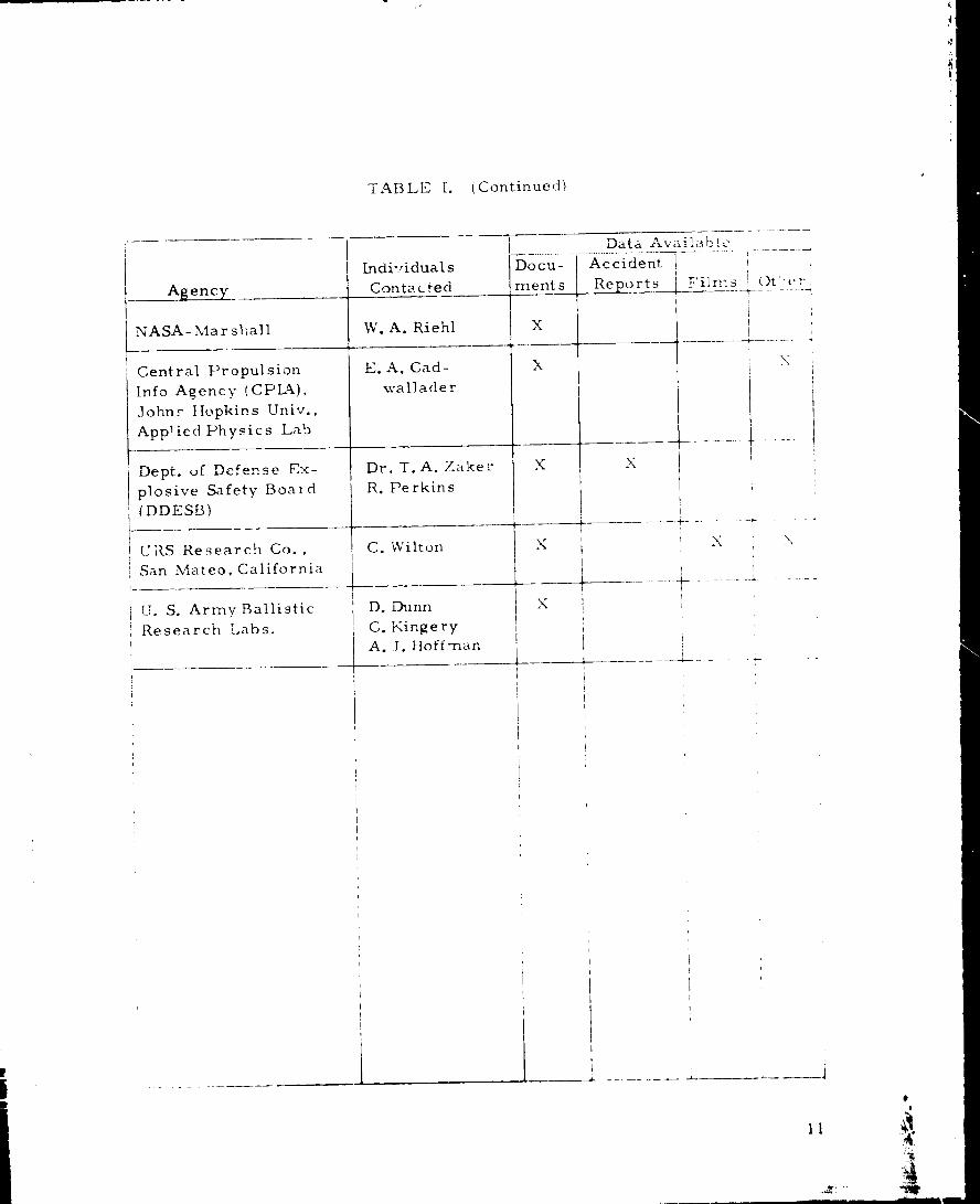
TABLE [. (Continued)
_ Agency.
NASA- Mar shall
Central Propulsion
Info Agency (CPLk),
Johns Hopkins Univ.,
Applied Physics Lab
Dept. of Defense Ex-
plosive Safety Board
(DDESB)
URS Research Co.,
San Mateo, California
U. S. Army Ballistic
Research Labs.
Individuals
Contacted
W. A. Riehl
E. A. Cad-
wallader
Dr. T. A. Zaker
R. Perkins
C. Wilton
D. bllfill
C. Kinge ry
A. 7. Hofiman
Data Availab ',c
-Do cu- Acc!dent ]
ments Rep_ Films
X
X
X
X
X
X
Ot" c :"
11
copies of accident reports which would provide useful fragmentation data, andhave not been able to include these data in our review and further analysis.
As documents and data were received at SwRI as a result of our initialvisit to ASRDI, our subsequent visits to other agencies, and our library andDDC literature searches, we reviewed each document, completed ASRDIform 102A for the documents and forwarded these forms to ASRDI. A total of168 documents were reviewed ._nthis manner, with various SwRI staff mem-bers completing the Forms 102A for documents which fell wi'chin their tech-nical specialties.
We believe that we have discovere4 and reviewed most of the pertinentliterature, data, and accident reports pertaL_.ing to fragmentation of liquid pro-pellant rockets and vessels. There is, however, one possible exception.There may be a body of fragmentation data in accident reports in the Air ForceInspection and Safety Center at Norton Air Force Base, California, which wecould not review or obtain for legal reasons. These reports were reviewed bystaff members of the Center, and we have been notified that they contain noda,a which could be used in our study. Because we were not allowed to re-view _he reports ourselves, we have no way of comparing them with otheraccident reports which have provided usetul data, nor do we know [he criteriaapplied by Norton personnel in a_sessing the potential value o _ specific reports
to this project.
12

If. DETERMINATION OF BLAST YIELD
A. General
A prerequisite to estimation of fragmentation effects for liquid ;_ropel-
lant explosions is the estimation of energ' released during the explosioa,
which is synonymous with explosive yield. Furthermore, to properly estimate
fragment velocities of appurtenances which can be accelerated by the blast
wave from propellant explosions, one must know the time histories of various
physical parameters describing the blast wave as a function of distance from
the explosion. We must therefore consider blast effects in some detail, even
though this is a study of fragmentation.
Accidents with liquid propellant rockets, both during static firing on a
test stand and during launch, have shown that liquid propellants can generate
violent explosions. These explosions "drive" air blast waves, which can
cause direct damage and can accelerate fragments or nearby objects. The
launch pads at the Air Force Eastern Test Range (_YTR) have for a number of
years been instrumented with air blast recorders 1o measure the overpres-
sures generated during launch pad explosions, so sonle data are available on
the intensities of the blast waves generated. Such measurements, and the
common practice in safety circles of comparing explosive effects on the basis
of blast waves generated by TNT, have led to expression of blast yields of
propellant explosions in equivalent "pounds of TNT". (Although a direct con-
version of pounds of TNT to energy can easily be made - I [b of TNT equalsPF,_
1.4 x 10 6 ft-lb - this is seldom done.)
Liquid propellant explosions d_ffer from TNT explosions in a nu_ber of
ways, so that the concept of "TNT equivalence" quoted in pounds of TNT is far
from exact. Some of the differences are d_scribed below.
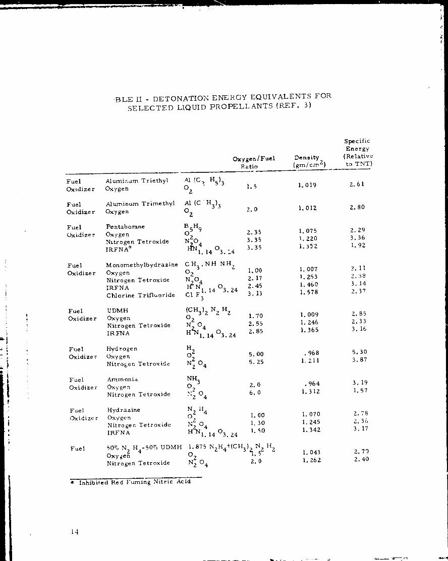
(l) The specific energies of liquid propellants, in sto_chiometric
mixtures, are significantly greater than fo-' TNT (specific
energy is energy per upit n_ass). Table II, taken from ref. %,
gives specific energies fox" a n._mber of !iqt_id-propella:_t/
oxidizer mixtures, as ratios to TNT specific ,nergy. Nott, thai
alt of the energy ratios in Table II are gr_,ater than 1, and
range as high as 5. 3.
(2) Although the potential explosive yield is very high for liquid
oropellants, the at__ual yield ts n_uch lower, because' prop_.llant
'and oxidizor are never intimately mixed in tho proper propor-
tions before ignition.
'BLE II - DETONATION ENERGY EQUIVALENTS FOR
SELECTED LIQUID PROPELLANTS (REF. 3)
Oxygen/Fuel Density 2Ratio (gmic_)
Fuel
Oxidize r
Fuel
Oxidize r
Fuel
(Oxidize r
Fuel
Oxidizer
Fuel
Oxidizer
Fuel
Oxidizer
Fuel
Oxidizer
Fuel
C)xidize r
Fuel
Aluminum Triethyl _i (C_ HS) 31.5 1.019
Oxygen O z
Alunninum Trimethyl AI (C H3) 3
Oxygen O z 2.0 I. 01Z
Specific
Energy
(Relative
to TNT)
2.61
g.80
Pentaborane B 5H9
Oxygen 0 2 2.35 I. 075 2. 29N O 3 35 1 220 3 36
Nxtrogen Tetroxide • " "
!RFNA* _4.14 O3.=4 3.35 i.352 1.92
Monomethylbydrazine CH 3,NH NH ZOxygen O z I. 00 I. 007 2. I I
Nitrogen Tetroxide N 04 Z. 17 1.P53 2.38Z. 45 1. 460 3. 14
IRFNA H_NI" 1403"24 3.13 1.578 2.37
Chlorine Trifluoride C! F 3
UDMH (CH3) z N Z H 2
Oxygen O 2 I. 70 I. 009
Nitrogen Tetroxide N_ 0 4 2.55 I. 246
IRFNA HZNI. 14 03.24 Z. 85 I. 365
Hyd r o ge n H 2
Oxygen O 2 5.00 .968
Nitrogen Tetroxid¢ N 2 0 4 5.25 1. Zil
Ammonia NH 3Oxygen O 2. 0 . 964
_.2 1 312Nitrogen Tetroxide '2 04 6.0 •
2.85
Z.33
3. 16
5.30
3.87
3.19
1.57
Hydrazine N2 }{4
Oxygen 0 2 I. 00 I. 070 2.78
Nitrogen Tetroxide N- 0 4 I, 30 I. 245 2.36
IRFNA H4N1. 14 03. 24 1. 50 1. 342 3. 17
H3)- N Z H 250% N 2 H4-50% UDMH 1.875 NzH4+(C LI.5 1.043Oxygen O 2
Nitrogen Tetroxide N 2 04 2.0 1. 262
* Inhibited Red Fuming Nitric Acid
2.79
2.40
14
(3) Confinement of propellant and oxidizer, and subsequent effect
on explosive yield, are very different for !iquid propellants and
TNT. Degree of confinement can seriously affect explosive
yield of liquid propellants, but has only a secondary effect on
detonation of TNT or any other solid explosive.
Tt_e geometry of the liquid propellant mixture at time of ignition
can be quite different than that of the spherical or hemispherical
geometry of TNT usually used for generation of controlled blastwaves. The sources of compiled data for blast waves fron_ TNT
or Pentolite such as references 2 and 3, invariably rely on
measurements of blasts from spheres or hemispheres of ex-
plosive. The liquid propellant :-r_ixture can, however, be a
shallow pool of large lateral extent at time of detonation.
(5) The blast waves from liquid propellant explosions show differ-
ent characteristics as a function of distance from the explosion
than do waves from TNT explosions. This is undoubtedly
simply a manifestation of some of the differences discussedTI
pre-ciuua,y, but it dues change the "TNT equivalence of a
"liquid-propellant explosion with distance from the explosion.
Fletcher (ref. 37) discusses these differences and shows them
graphically in Figs. 1 and 2. These differences arv very evi-
dent in the results of the many blast experiments r_port_'d in
Project PYRO (refs. t5-17). They have caused the coinage of
the phrase "terminal yield", meaning the yield based on blast
data taken at great enough distance from the explosion for lhv
blast waves to be similar to those produced by TNT explcJsions.
At closer distances, two different yields are usually reported:
an ovtrpressure yield based on equivalence of side-on peak
overpressures, and an it,_pulse yield based on equivalence of
side-on positive irnpulqes.
There exist at present at least thr_.-," methods L,r ..stimating yield from
liquid propellant explosions, which do not necessarily give the sa_,,, predic-
tions. One method is based on Project PYRO resu]ts (refs. 15-17), and the
other two are the ':Seven Chart Approach" and the "Matttematical Model' of
Father and Deese (ref. 23). We next discuss eactl n_ethod and some back-
ground information.
B. Project PYRO and Related F×periments
Project PYRO was a joint NASA/USAF project conducted durin_ the
period 1965-1967 with the purpose of determining the blast and thern_al char-
acteristics of three iiquid propellant combinations in most common use in
I'5

2.0-
,-J
>-
N
,,(
_E
OZ
1.5
1.0
0.5
FIGURE 1
PROPELLANT IMPULSE
PRO_PEL_I PEAK PRESSURE
l I ....i I10 20 30
RADIUS, ft
I I J5O 60 IO
NORMALIZED PRFSSURF AND IMPULSF YIELDS FROM EXPLOSION
OF N204/AEROZINI_ 5,3
Tm--_I
/I
PROPELLANT_
(a) (b) (c) (d)
FIGURF 2 . REPRESENTATIVE SHOCK IkA..f>ULSES SItOWING COALE'ACENCE OF SHOCK WAVES FROM
DISSIMILAR SOURCES _TAG_?S a) THROUGtt d)]
16

i
!
military missiles and space vehicles. It included 270 tests w;th iotal wt, ights
of p:.opellants ianging from 200 lbnl to 100, 000 lb m Most of the tests wcrc
conducted at the Air Force Rocket Propulsion Laboratory (AFRPL) at Edwards
AFB, California. Prime contractor for much of the effort was URS SystcTllS
Corp., Burlingame, California. The project was supervised bv a Steering
Committee of representatives from several NASA centers, the Air F'orcc'
Eastern Test Range. and the Sandia Corp.
The emphasis in Project PYRe was almost exclusively experimental.
Tests were designed to simulate various types of accidents which could cause
mi:_ing and ignition of the proFellams. The primar.v blast instrun_entation was
an array of blast pressure transducers whose outputs as functions of tin_c wet,'
recorded on magnetic tape. (Although fragmentation effects were incidcntai to
the program objecti\es, high-speed motion picture can_eras p}_otograpl_'d tl',ost
of the tests, and our data on fragment velocities are all obtained froP.', lhcse
films.) The results of the progran_ were reported in a threc-\o!unn_: final
report, with Vol. ! (ref. 15) describing ti_e F,rogra_n_ e. nd _ixing overall rose,Its,
Vol, II (ref. 16) giving detailed test data, and Vol. III {ref. 17) gixing prrdic-
tion methods based on the prograna results• In the PYRe effort, thrc_' basic
types of accidents were .._imulated. The first t/pe consisted of failure of an
interior bulkload separating fuel and oxidizer in a missil( stage. This \\:_s
termed Confinement b.v the Missile (CBM). The second type of accid_ nl
included in,pacts at various velocities of t}" missile on the _round, _vith ;tll
tankage ruptured, and subsequent ignition. I!-,is was tern_cd Confi nt•n_cnt l_v
_e Ccound Surface (CLsGS). Ttne third t.vpe was High Velocit} I_l_,Pac / (ttVi)
after launch.
Although Project PYRe generated n/uch more da_a on cxl)losi',c vi_,l:is
cd liquid propellant explosions than all prcvi,ms st_dics cor_bincd, sc\_,ral
..arlier c, xuerim_ r_tal programs did give ,ts_iul data arid should bc _'_cnliuncd
here. " ,-thur D. Little, Inc., (r_'f. Z4) conducted a series of bl, st t,,sls sir:-
u!ating spills and ignition on th_ !round of \-ariel,s ,-o:_binations el })r(,_)cllants
in +he Saturn _-chicles. The tcstS were ,icsif,.ncd to prud,_c_: thc tl?;:txi?_?kl:l?
possible bi_st .viei-t for this type o_ accident ,vith lhorougb mixin,a of fu,.ls and
oxidizer -,c_:_. d_ia',s of ignition until such n_ixin_ was co,-__pl(.tc. Ti',_.s_' ,'_n,_n_-
n:eu:" -;:_ve_;ti_ators r(t_orted bl :_ waxc characteristics identical to th_sc fro:"
I'2_ [" exp!osicr, s in the overpress_re range of their ,_,asur_,_ '.nts ; 1()(_ _,si),
and blast yields ranging fr:)n_ (I. 27 l_ 1. '_8 1!) TNT/lt_ propcllat_t. Tiq_,_ )tlb{_
estin_atcd nnaximuna potential yields (e\'_'n includina effects of tfl_r})tzI "tlill'_, of
ut-_burned fuel wttl:] oxygen in the air) of considcrabl' less than in 5_I_I_' II.
Their pr(,dicted :_-_axin'_a are given in Table III.
17

TABLE III
PREDICTED MAXIMUM BLAST YIELDS (REF. 24)
Propellant
RP- i/LO 2
LHz/LO 2
RP-I/LOz/LH z
Ratio of Blast Energies,
!b TNT/lb Propellant
1.25
3.70
2.75
Another experimental effort prior to PYRO is reported by Pesante and
Nishihazashi (ref. 25). These investigators measured the blast waves gener-
ated by fuels and oxidizers which were violently mixed by explosively shat-
tering dewars containing one component, while the dewars were immersed in
a bath of the other component. Blast yields ranging from 0.Z3 - 0.80 Ib TNT/
Ib propellant were obtained in these experiments. {These tests also included
attempts to measure velocities of objects pla_.ed near the blast wave, but no
useful data were obtained. }
The final set of tests prior to PYRO is apparently a series reported by
Gayle, et al. (ref. 26). Fuels and oxidizers were mixed by several different
methods (anticipating the two primary simulation methods in PYRO), and blast
wave properties measured as a function of distance. These investigators
showed a much greater spread in blast yields for other methods of mixing than
spill tests, ,_'ith much smaller yields being observed in most tests for simu-
lated bulkhead rupture, etc. Yields for LH2/LO Z combinations were most
affected by the change in methods of mixing, being no greater than 0.014 lb
TNT/lb propellant for any of the tests.
From the test results reported in references 15 and 24 through g(), a
number of observations can be made regarding blast yields from liquid propel-
lant explosions.
(l) The yield is very dependent on the mode of ,nixing of fuel and
oxidizer, i.e., on the type of accident which is simulated.
Maximum yields are experienced when intimate mixing is
accomplished before ignition.
(2) Blast yield per unit mass of propellant decreases as total pro-pellant mass increases.
(3) The character of the blast wave as a [unction of distance differsbetween propellant explosions and TNT explosions, as notedbefore. There is some evidence that these differences arcgreatest for low percentage yield explosions. (They were notobserved in tests of re[. 24, for example.)
(4) On many of the LHz/LO 2 tests (regardless of investigators),spontaneous ignition occurred very e_.rly in the mixing process,resulting in very low percentage yields.
(5) Yield is very dependent on time of ignition, even ignoring thepossibility of spontaneous ignition.
(6) Yield is quite dependent on the particular fuel and oxidizer beingmixed.
(7) Variability in yields for supposediy identical tests was great,compared to variability in blast me0surements of conventionalexplosives.
The PYRO blast yield prediction methods given in reference 17 are a
set of "cook-book procedures" for estimating blast pressures and impulses for
specific types of liquid propellant accidents and specified geometric and initial.
conditions. Inherent in the prediction method is scaling of ignition time ac-
cording to t/W 1/3 Types of accidents considered ate confinement by missile
(CBM), confinement by the ground surface (CBGS), a_d high velocity impact
(HVI). Equivalent TNT yields are determined and estimates of overpressure
and impulse made based on compiled blast data for TNT (re[. 2), with a cor-
rection factor for impulse to account for the difference between TNT and liquid
propellant explosions. Unfortunately, we feel that the prediction methods
given in reference 17 are oversimplified (for example, they use discrete and
different correction factors for impulse for different ranges of scaled dis-
tances, whereas the data in references 15 and 16 show a continuous variation
in impulse with ;caled distance), and they are based on a scaling of ignition
time which is dubious, i.e., not proven by experiment (see Apt:,endix A). The
methods of reference 17 also are designed to give upp(r-bound estimates of
blast effects, rather than most probable estimates. The possioility of limita-
tion of blast yield by early autoignition when large ma._ses of propellants are
mixed is ignored in the PYRO prediction schemes. Considering the careful
and well-documented experin:ental work reported in raferenc_'s 15 and 1,,, th(,
prediction methods of reference 17 are quite disappointing.
19

C. Work of Farber and Deese
More or less concurrent with the PYRO work, but continuing to thepresent, Farber at the Uniw:rsity of Florida and Deese at NASA-Kenned_ havecond'acted a combined theoretical and experimental program of the study of thephysical and chemical processes involved in mixing, ignition, and explosion ofliquid rocket propellants. The results of this work are reported in a numberof papers, with the efforts through October 1968 being best summarized andreported in reference Z7. Later work is reported in references 28 through 30.
In the work reported in references 28-30, the problem o:: mixing, igni-tion and explosion of liquid rocket propellants is subdivided into a nurnber ofsub-problems, and each sub-problem studied more or less independently. Theresults of the subsequent analyses and experiments are then combined in sever-al prediction schemes for explosive yield, of which the most detailed is the"Seven Chart Approach" of reference ;3.
The ,;ub-problems into which the overall problem was divided by Farber
and Deese were:
(1) Determination of the ,_otential maximum, explosive yield obtain-
able if the liquid propellants present were mix._d in an optimum
manner (yield potential function)
I')_t..)
Determination of amounts of propellant which woald be mixed as
a function of time after "spill" (mixir. g functic:.n)
(3) Determination of most probable time'_ 9f delay _f ignition and
detonation (delay and detonation times)
Y':_rber and Deese (ref. 23) also evolved a method o_ err, piric.ally fitting to
experimental data a four-.parameter probabilit} function vti:h would predict
th: - probability of explosive yield to various levels of conf:dence, and have
more recently evolved an hypothesis of a critical mass of ._fixing propellants
for which autoignit'on is certain.
The yield potential function is calculated by .Farbet', et al (ref. 27) on
th,. basis of chemical kinetics considering boiling and fre _zing of fuel-ox_.dizer
ccmoonents as _ function of time after an assutned irstartaneous mixing.
tteat values for the various chemical reactions which co,.ld occur at various
times, considering s, tates and amounts of reactants F,res_nt, are then cal,tu-
rated. Some rtetails of the manner in which these calcu'.ttions are made art.
given in reference 27, and a typical result for an initial mixture ot LO2/I,H2/
RP-I is -c;hown iv. Figure 3. There are no experimental data which -lirectly
confirm such theoretical calculations of the yield function.
gO
,L
4
,r
¢
i
I
o
d d
o
d
o
o
o
n_q '3_JNIXIW 30 (]NNOd _J]cl 35V373U AO_J3N3
!
F_Z<
0
2
Z
©
<
©
<
7_
X x
_5
21
The mixing function, expressing the fraction of mass of fuel plus oxidi-
zer actually mixed as a function of time after spill, is the best esl:ablished of
Farber's sub-problems. No less than four experimental methods were used to
establish this function (ref. 27). A typical mixing function is shown in
Figur_ 4. This function peaks as mixing becomes more complete, and then
decays because the mixed propellant evaporates. An optimum time for ignition
(optinaum in that it will _.)roduce maximum explosive yield) is therefore heavily
deperdent on this function.
The least well-determined of the sub-problems is the definition of ex-
peL.ted delay times for ignition. A statement from reference 28 appears up-
Drop:late "Th_ ignition time for prediction purposes, can be a controlled
%-clue, a kno'_'a "._al_'-e be..,_ed upon the characteri';tics of the propellants, a
statistical value with _.c,n£idonce limits, or it can be a value deternqined by the
critical mass method .... ". In o_b.er words, the ignition time is apparent!y
anyone's best guess. It is clea_- from the results of liquid propellar,t ,x, ixing
tests that autoignition alway.s occurs for mixing of z,.!fficiently large quantities
of propellants Farber (refs. 27-30) has hypotaesized that a source oi ignitio_a
whizh is always present: upon mixing is electrostatic build-up of voltage and
subsequent ,zlectricaldischarge through a gas bubble, and that a critical nmss
exists for a given propellant mixture and set of initial conditions which pro-
rides a short upper limit on ignition time, and therefore an upper !.imit on
ext,losive yield. Recent experimental work by his group (ref. 29) is directed
sp, cificall), toward measurement and verification of this hypothesis, and w_r_-
fic._tion is claimed (although not conclusively proven) by work reported in
re!erence 30.
The two prediction methods developed oy Farber, et al, are termed the
"Seven C!_art Approach" and the "Mathematical Model". Each will give an
e'timate of explosive yield y , expressed as a fraction of the total heat of
c,mabust!.on ofa stoichiometric mixture of fuel and oxidizer. In the "Seven
Chart A,_proach", a graph such as Figure 3 i_ normalized by" dividing by the
n_axir'c, um heat value reached by the mixture, and then converted to a norme,1-
i'ed yield potential yp versus time plot such as Figure 5. The fractionrlixe_ x as a function of time (Figure 4) is then multiplied by yp at approxi-
t_ate times to give expected yield y (see Figure 6). Finally, some estin_ated
!gnition time, with suitable confidence limits, is superimposed on Figure 6 to
;ire tee final estimate of yield y . (Note that only four charts are discussed
'acre. The remaining three charts in the seven-chart method shov¢ intermedi-
ate steps).
The "Mathematical Model" method (ref. 28) consists of fitting to exper-
ir-:ental data a _elation'_hip betv'een normalized yield y and mixing function x
of the form
Z2
G3XIW NO11_)¥_I'I
0
i_-
0
z_0
Z<
'_N
Z_
0
4r4
©
z3
!
!
24
c_
t----_ i ! t !
Z0
<
<
Z
"IVl 1N310d OI31A
6
÷
I
dX. AIA '(]131A f131O3dX3
t_
0?,..)ILl
ZI
L.m..l
I
I-.-
A
[_
_2
Z0
2:0
Z<
Z0
2:G
0
Z<
C
b,,,,,l
£

t
b d (Z)- X
Y b+c
where b, c, and d are parameters to be adjusted. An auxiliary function is
also introduced which inserts a fourth parameter, a . Using the physically
realistic limits of zero yield for zero spill, and a maximum for y when
x : I which is defined by the fraction of mixed propellants which represent
stoichiometry (y< ]), fixes the parameters b and c . Farber originally used
data from reference 24 to estimate the parameter d _ and has not changed this
parameter since. So, essentially only the parameter a remains to be varied,
and Narber claims that the parameter a represents a "scaling parameter"
related tototalmass of propellants. With parameters chosen from fitting data
of reference 24, F'arber claims (ref. 28) prediction of upper bounds on explo-
sive yield which cover all available data through 1969 (see Figure 7).
After review of the work of Farber, Deese and co-workers, we feel
that t.heir efforts have their strengths and weaknesses, just as does the PYRe
work. The greatest strengths are the excellert physical insight into the com-
plex processes which occur during mixing and ignition of liquid propellants,and the division o_' the complex overall problem into sub-problems which can be
studied separately. Narber and co°workers were also apparently the fir-_t to
realize that explosive yields for large quantities of propellants were always
limited by earl_ autoignition. The primary weaknesses lie in lack of experi-
mental verification of the physical processes, sometimes doubtful clain_s of
usefulness or applicability of limited test t_chniques or data':" and reiteration
of the same material in succeeding reports. The two methods for prediction
of blast yield are well described and understandable, but both gi_e an estimate
of explosive source energy without consideration of the nature of the' blast
waves generated by liquid propellant explosions which were evident in Project
PYRe. It !.s also not clear how the critical mixin_ functioc, such as Figure 4
is obtained for various types of full-scale accidents or tests, or how _.i ;,s
scaled from laboratory experiments.
D. Fstimation o[ Blast Wave ["ropert .s
We present her,' methods of estimating blast yields and blast wa_e
prop-,rties for liquid propellant explosions, based prir:arilv on PYRe results
and on the work of Farber and Deese. Although ',ur pred,ct :m metbuds retain
many of the features of the previous work, they a'_so dieter somewhat where w.
feel chan_es art' appropriate. Fur,hermore, factors _'hich appear to have :
In particular, respor, se times, tirrae resolution and identificatior, of :4_vsical
phenomena from therrT,ocouple grid n_easuremeats claimed it. ,'eference Z7
seem doubtful.
Z6
5
1.0_YRO Data Q A ComputedA Experimeatal
uLJ AverageValue
0._ - ADL ,Spill Tests (J)
_ _ _ . _ A SelfoII
e-4
Ignit ion
PROPELLANT WE!GHI, Ib
Limit)
FIGURE 7. ESTEvIATED EXPI,OSIVE YIELD A3 A FUNCTION
OF PROPELLANT WEIGIIT {PEF. ZT)
27
t¢
secondary effect on blast yield, such as L/D ratio of tankage, are ignored.
The coecept of "TNT equivalency" is used only to estimate energy of a liquid
propellant explosion, and not to predict detailed blast wave characteristics.
Blast is strongly dependent on type of propellant, type of simulated accident,
in-Fact velocity, and ignition time, so these factors must be accounted for in
estimating blast wave characteristics and yield.
Throughout the PYRO work, blast yield is expressed as percent yield,
based on an average of pressures and impulses measured at the farthest dis-
tance from the source when compared to standard, reference curves (ref. 2)
for TINT surface bursts (terminal yield). Hopkinson's blast scaling is used
when comparing blast data for tests with the same propellants and failure con-
ditions, but different mass of P rlo/P3ellant. So, the blast parameters P (peak_side-on overpressure) and I/W (scaled impulse) are plotted as functions
of R/W 1 /3 , (scaled distance) after being normalized by- the fractional yield.
This procedure is equivalent to determining an effective weight of propellant
for blast from:
Y (3)W = W x
T 100
where W T is total weight of propellant, Y is terminal blast yield in percent,
and W is effective weight of propellant. Because the data are normalized by
comparing to TNT blast data, the effective blast energy E can be obtained by
multiplying W by the specific detonation energy of TNT, 1.4 x 106 ft lb/lb m.
We -viii use smoothed curves through the scaled PYRO blast data, and Equa-
tion (3), to obtain blast wave properties for any particular combination of
propellants and simulated accident. We will consider each propellant combina-
tion separately.
1. tt_pergolic Propellant - The hypergolic propellant in widest use,
and used in the PYRO tests, is a fuel of 50_]c N z H4-50°]c UDMH and an oxidizer
ot N 20 4 in a mass ratio of 1/?.. Hypergolic materials, by definition, ignitest,ontaneously on contact, so it is not possible to obtain appreciable mixing
before ignition unless the fuel and oxidizer are thrown violently together.
Ignition time is therefore not an important determinant of blast yield for hyper-
golics, but impact velocity and degree of confinement after impact are impor-
tant factors. Project PYRO results and resulting prediction methods which
are given in references 15-17 concentrate on these factors and can be used
directly to obtain estimates of blast yield. The only modification which we
propose is to use smoothed curves from PYRO results for peak overpressures
and impulses, rather than multiplying factora.
Z8
'I:he procedure is then as fo]lows:
(1) Consider failure mode, or impact velocity and type of surfaceimpacted.
(2) Obtain terminal yield Yreference 16}.
(3) Calculate Wlant and Y .
(4) At distancesR/wl/3
in a/c from Table III or Figure 8 (from
from Equation (2) knowing tGtal weight of propel-
R of interest, compute Hopkinson-scaled distance
(5) From appropriate smooth curves in Figures 9and 10, read peak
overpressure P and scaled impulse I/W 1/3 Multiply scaled
impulse by W 1/3 to obtain I .
TABLE IV - ESTIMATE OF TERMINAL YIELD (REF. 16)
FAILU RE MODE
Diaphragm rupture (CBM)
Spill (CBGS)
Small explosive donor
Large explosive donor
Command destruct
310-ft drop (CBGS)
TERMINAL YIELD RANGE (%)
0.01 - 0.8
O.02 - 0.3
0.8 - 1.2
3.4 - 3.7
0.3 - 0.35
~I. 5
m
ESTIMATED UPPER LIMIT
1.5
0.5
2
5
0.5
3
Note that the blast yields are very low (a fraction of one percent to a
few percent) for all but high velocity impacts, which is not surprising in viem'
of the small amount of mixing which is possible before ignition. Possible
error in estimation of yield is also substantial, as can be seen from the
ranges of yields in Table IV and data scatter in Figures 8, 9 and 10.
2. Liquid Oxygen-Hydrocarbon Propellant - The second propellant
combination which we will consider uses Kerosene (RP-1) as a fuel, and liquid
oxygen (LO 2) as the oxidizer in stoichiornetric mass ratio of 1/2.25. Because
this liquid propellant is not hypergolic, considerable mixing can occur in
Z9
" PYRO DATA
' 60[" 0 2oo lb F_T PAl)raTA
/ • 1000 lb FLAT PAD DATA
I_ 200 lb DEEP HOLE DATA
i i IOOO i b DEEP HOLE DATA
50 --... HARD SUP.FACE•. • SOFT SURFACE
- _ _ ........................_ eooo o°°°le
i I ,.... mooo e°
_ oN
i! ,• i
! ' ,6OO
_ i _o
I
k
!
iI
i
i
Ii
,m
t_
a_"
I.I.I
r_
Q.
I0
1.0
D
x
PYRO DATA
HIGH-VELOCITY'IMPACT TESTS
OTHER TESTS
"\\ x_ ._TNT DATA AND HIGH
/ VELOCITY IMPACT
PROPELLANT DATA
\\.x"
" "X\\. _x,,_.x
\
PROPELLANT FAILURE --/Ix'X,"
X
\\\,\
__MODES OTHER THAN _"
HIGH VELOCITY IMPACTS "\_.Q
I I I I t i
I0
1/3 1/3SCALED DISTANCE R/W , ft/Ib
100
FIGURE 9 . PRESSURE VS SCALED DISTANCE FOR
HYPERGOLIC TESTS
31
40
Or_--...,.
e,--4
--......
¢.)(%)L#)
EI
.m
I0
1.0
PYRO DATA
fl I GH- V ELO CI TY- IMPACT
\
I , , i I l , , 14 I0 100
SCALED DISTANCE R/W I/3, ft/IbI/3
\\
FIGURE 10. SCALED POSITIVE IMPULSE VS SCALED DISTANCE
FOR HYPERGOLIC TESTS
i 32
J

various types of real or simulated accidents, and time of ignition after on'_et of
mixing is an important determinant of blast yield. Other important parameters
have been shown by the PYRO and other results to be the mode of failure or
simulated accident, impact velocity, and propellant mass or weight. Less
important parameters appear to be geometry of tankage expressed as a length-
to-diametel (L/D) ratio, propeIlant orientation, and area of rapture of interior
bulkhead for CBM case. The estimation methods which we give here are
based largely on the PYRO test results, but also include conclusions and/or
physical reasoning of our own and of Farber and other investigators.
For the case of mixing and an explosion within the missile tankage
(CBM), time for ignition at, a mass of propellant are the principal determinants
of blast wave properties. The scaling of ignition time assumed for PYRO is
no__j_tproven by the PYRO test results (see Appendix A), so we simply plot asmooth curve through PYRO results for blast yield Y as a function of time t
in Figure ll. We also use Farber's physical reasoning in plotting this curve,
i.e., for zero time for mixing, yield must be zero, and for long enough time,
yield must decrease. A direct plot against ignition time is used, independent
of mass of propellant, because it fits the data as well as scaled time plots and
also serves to indicate that scaling of ignition time has not yet been verified
experimentally. Once blast yield Y has been determined from Figure l; for
an assumed _.gnition time, effective weight of propellant W is then calculated
from Eqtation (3) for known Y and W T , and blast pressures and impulses
are obtained from fits to PYRO data in Figures 12 and 13, in exactl,.: the same
manner as for the hypergolic propellants.
For simulated fall-back on the launch pad (CBGS), impact velocity as
well as ignition time are important parameters in estimating blast yield.
PYRO prediction methods included fits to scaled time parameters and to im-
pact velocity to a fractional power close to one. As stated before, time
scaling is not proven by the data. Also, linear dependence on impact velocity
is simpler than a fractional power close to one and fits the data just as well.
A suitable fit of maximum yield Ym to impact velocity, agreeing with curve
A of Figure 5-41 of reference 16, is:
z. 0s (4)y = 507c + 0 < U I < 80 ft/sec
m (ft/see) UI' - -
where Ym is expressed in a/r, and U I is ia ft/sec. Blast data for this case
from reference 16 are normalized with respect tc Ym by the factor
X . 100/Ym , and plotted versus ignition time in Figure 14. The smooth curve
through the data can then be used to predict percent yield using Ym from
Equation (4) fo" impact velocity U I . Again, using Equation (3}, W can t_e
f_und and blast parameters determined from suitable fits to PYRO data, which
are given here as Figures 15 and 16.
33
' _J. tl
• ,
34
m
>-
I--
6O
5O
4O
3O
2O
- 0
0
0
0
0
I0_ o
0
0 2OO
0
0
o-- 5OOO
FIGURE II. IGNITION TIME VSYIELD LOz/RP-I CBM
o-- 73OOO
O O
I I I J400 600 800 10O0
IGNITION TIME t, msec
%
400
W
.<
_t
F4.
,m
e-,
l.z.l
rv'
l.l.J
n,,,
O
CL.
100
n
m
1C-
1.C
DATA
PROPELLANTDATA
PYRO DATA
O 25,000-LB DATA
• ALL OTHER DATA
1.0 10
SCALED DISTANCE R/W1/3, ft/Ib 1/3
FIGURE IZ. PRESSURE VS SCALED DISTANCE FOR
LOz/RP-I CBM CASE 35
lu0

J
I
(._-...,...
u
--.....,.
f_(1)
EI
--,.....
....,.,..
c_..-I
r_
_Em
L.I.I
m
I,,,-
0r_
(,.)
100
b,,
10-
I.C l
FIGURE
PYRO DATA
0 25,O00-.LBDATA• ALL OTHER DATA
O
;'ROPELLANTDATA
TNT DATA
I
1.0
I I I I [ _ L l
10
SCALED DISTANCE R/W 1/3, ft/Ib 1/3
13. SCALED POSITIVE IMPULSE VS SCALED DISTANCE
FOR LO z/RP-I CBM CASE
Iu0
36
100-
80-
6O
Y-tO0.
Ym
40
2O
0
0
FIGU RE 14.
O
O
O
O O
O
O
O
O
O
O
O
o--1220
O--1835
400 600 8IGNITION TIME t, msec
I
1000
IGNITION TIME VS NORMALIZED YIELD
LOz/RP- I CBGS
_7

*e._ ¸ '
om
lO•
38
\\
0
• ALL OTHER DATA
TNT DATA100-
LPROPELLANT "
_ DATA " o_._
__ _',_
1.0 t -
I 1
1.0
PYRO DATA
25, O00--LB DATAi.-_RGE- PO OL-D _AMETER DATA
1 i 1 I I l L , l
10
SCALEDDISTANCE RIW 113, ftllb 1/3
FIGURE 15. PRESSURE VS SCALED DISTANCE
FOR LOz/RP-I CBGS-V CASE
1
100

PYRO
o
-PROPELLANT DATA "_ 100- . /-
I
"_:_. _ _. o"
-- Q OI • e• •
_ • •g •
_ TNT DAT '.... ----" - • ogal •j _ I0 . . _....
- "_'_KL"_I __ ',o,,_._ _
_ ".._.':
I!
|._ _
I , 1.0 10
_, SCALED DISTANCE R/W 1/3 ftllbl/3t
DATA
2S,OGO-LB DATA
ALL OTHER DATA
\%, .
FIGURE 16. SCALED POSITIVE IMPULSE VS SCALED
DISTANCE FOR IOz/RP-L CBGS-V CASE
100
39
.%
3I
I
In high velocity impacts of this propellant, the situation is somewh_-t
simpler because there is little ignition delay and therefore only impact veioci-
ty affects yield. Prediction methods from reference 16 can then be used to
estimate yield Y (see Figure 17) and blast parameters obtained from Equa-
tion (3) and Figures 15 and 16.
3. Licluid Oxygen-Liquid Hydrogen Propellant - The final propellantcombination is the entirely cryogenic combination of liquid hydrogen (LH z)
fuel and liquid oxygen (LO z) oxidizer in stoichiometric ratio by mass of 1/5.
The rationale for predicting blast parameters for this propellant com-
bination is identical to that for LO2/RP-I. For the CBM case, Figure 18
gives a plot of ignition time versus yield. After determining W from this
plot and Equation (3), one can enter Figures 19 and 20 to obtain blast wave
properties.
For the CBGS case, a linear fit of maximum yield versus impact
velocity gives
1.3s (5)Y : 10% + UI 0 < UI< 80 ft/secm (ft/sec) ' -- --
Using this equation to normalize ignition time versus yield, we obtain
Figure 21. From the curve in Figure ZI, we can find Y for a given ignition
time, and then obtain W from W T and Equation (2). Finally, blast pressure
and impulse are obtained from Figures _.Z and _3.
For high-velocity impact of this propellant, the blast yield is also
dependent only on the impact velocity, and the prediction methods of refer-ence 16 can be used directly. The curve in Figure 24 gives the yield Y , and
Equation (3) and Figures 22 and 23 will give predictions of blast wave proper-
ties.
4. Limit to Yield for Large Mass of Propellant - Any method of pre-
dicting blast yield must, it seems clear, provide an upper limit on yield with
increasing mass of propellant. All tests to date with large amounts of pro-
pellant have shown autolgnition sources which prevent mixing of even a large
portion of the oropellant prior to ignition. The simplest wayto incorporate a
limit is to use the limit curve of Figure 7 generated by Farber. The curve
labeled "average value" should probably be used for our purposes. Explosive
yield y in Figure 7 is only approximately related to Y in all of the precedingdiscussion, because Farber bases his yield on actual energy of combustion of
the propellant rather than TNT equivalence. But, considering the multitude of
other errors in these r_ethods, we can igno:e the difference and simply assuxne
that y = Y/100. (6)
4O

80
>.-
..Jl.J
>-
..J
Z
W.lI--
4O
SOFT
f _ARDSURFAC[,.
I i I i
0 100 2OO 3OO 4O0 5OO
IMPACTVELOCITY UI, ft/sec
1
FIGURE 17. TERMINAL YIELD VS IMPACT VELOCITY FOR
LOz/RP-I (REF. I6)
I41

7
i
!
O
80-
i°350q_
°
_O O O O O
i I I I
IGNITION TIME t, mse¢
FIGURE 18. IGNITION TIME V$ YIELD LOz/LH 2 CBM

r,,,"
400
I00TNT DATA
PROPELLANI •.X.X,'
10 DATA . \;.
° \_
1.0
I
1.0
.\.\
\
.\I i "'_, l i_ i
lO
113 ftllb 1/3SCALEDDISTANCE RIW ,
100
FIGURE 19. PRESSURE VS SCALED DISTANCE
FOR LOzILH z CBM CASE
43
i_ I

t
i
li,
,--4
m
EI
,w
u
..J
Q_
m
m
l--w
oa..
,-%l,J...J
O(/%
100
10
1.0
m
m
1.0 ]0
SCALEDDISTANCER/W1/3 ft/Ib 113P
FIGURE 20. SCALED POSITIVE IMPULSE VS SCALED
DISTANCE FOR LOz/LH Z CBM CASE
I
100
44

i.JIi
¢
|e
!
i.
IO0
8O
60
Y .loom
Ym
4O0
0
0
0
0
0
0
0
0
0 o
0
O0
00
0
00
0 0i 1 1
0 2OO 4OO 6OO 8OO
IGNITION TIME t, msec
o
0-- 1374
0-,-1524
0-- 1490
J
tOO0
FIGURE 21. IGNITION TIIvIE VS NORMALIZED YIELD LOz/LH ZCBGS
45
_.,-j
!
400
I00
•o
J
.,o• \o
PROPELLANT
\
\ •
• :\_" .\
DATA
\
PYRO DATA
o 25,000-LE DATA• ALL OTHER DATA
1.0
L l L J
10
SCALEDDISTANCE RIW113, ftllb 113
iL
46FIGURE ZZ. PRESSURE VSSCALED DISTANCE
FOR LOz/LH Z CBGS-V CASE
100 o
,, . PROPELLANTDATA
•" "K o
m
..I
(_
_Em
l--m
O
(_)
10 TNT DATA •
I0
PYRO DATA
0 25, O00-L_ DATA
• ALL OTHER DATA
, I i i I I 1 i\ I
10
SCALED DISTANCE R/W 113 ft IIb113P
FIGURE 2.3. SCALED POSITIVE IMPULSE VS SCALED DISTANCE
FOR LO2/LI'I Z CBGS-V CASE
47
1UO
i

i'
I
e
!
t
160
120
>.-
-,Ji,aJ
8O
.¢CZ
w 40t-.--
I I I
SOFT SURFACE -_
I I I I0 100 200 300 400
iMPACT VELOCITY UI, ft/sec
I I
HARD SURFACE
l
500
FIGURE 24. TERMINAL YIELD VS IMPACT VELOCITY FOR
LOz/LH z (REF. 16)
48
II!. DETER_MINATION OF FRAGMENT
VELOCIT Y DISTRIBUTI.ON
A. General
In our review of accident and test data for liquid propel)ant explosions,
we found no data on the velocities of fragments produced by these explosions,
outside of'-_ata a_,ailable in films of Project PYRO. Only the report by 7effers
{ref. 18) contained an analysis of fragment velocities, and this analysis was
based on a study of films of three of the PYRO tests.
The repository for all raw data, including f_lrns, fron] the extensive
series of PYRO tests is the Air Force Rocket Propulsion Laboratory at
Edwards Air Force Base, Galifornia. In visits to this agency, SwRI staff
members viewed all of the library of PYRO films and selected for data're-
duction films of 94 tests in which individual fragments were visible and could
be followed from frame to frame. These films were then loaned to the insti-
tute for measurement of fragment velocities. For most of these experiments,
several camera views of each test were available. Film speeds were accu-
rately known, with timing marks at known repetition rates impressed on the
edges of most films. The 94 tests for which we reduced fragment velocity
data represented a spectrum of propellant types, scale of test, and type of
simulated accident. In addition, reduced blast data and measured blast yields
are known for each experiment and reported in references 15 and 16.
Because the PYRO films constituted our raw data for detern_ination of
fragment velocity and because redv, ction of these data required more detailed
knowledge of test details than were available in references 15 and !6, we en-
gaged a consultant from URS Gorporation, prime contractors for PYRO. He
provided us with sufficient additional information, drawings of test arrange-
ment_, etc., to enable us to obtain accurate estimates of such needed informa-
tion as distance scales in the field of view of each camera and timing mark
frequencies on films. He also helped us resolve unexplained discrepancies in
reported PYRO test results.
Although the PYRO films provide all of our basic data 9n fragment
velocities and can allow correlation with measured blast yields, they do not
in general provide any data on fragment masses, shapes, or ranges. In only
one PYRO test were these parameters measured, and this test is the only one
for which any overall correlation af fragmentation effects conceivably can bp
made.
B. Reduction of Film Data
I. Camera Locations - Locations of the camera during PvRO tests
from which fragmentation data were obtained are shown in Figure 25.
49

I- ¢
!
,t
5O
---_/ : 340 °
4 _ TEST PAD
FIGURE ZS. PLAN VIEW OFCAMERA LOCATIONS DURINGl:rY RO TESTS
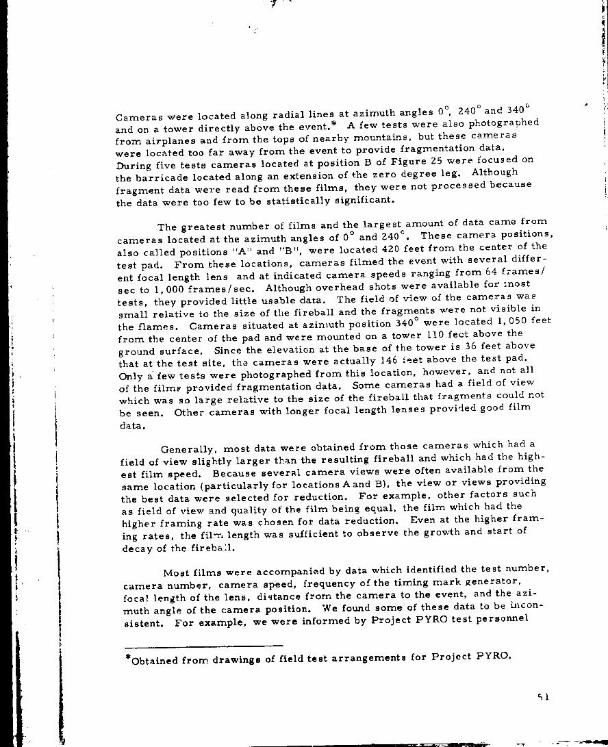
i"
Cameras were located along radial lines at azimuth angles 0 °, 240 ° and 340 °
and on a tower directly above the event.* A few tests were also photographed
from airplanes and from the tops of nearby mountains, but these cameraswere located too far away from the event to provide fragmentation data.
During five tests cameras located at position B of Figure 25 were focused on
the barricade located along an extension of the zero degree leg. Altbough
fragment data were read from these films, they were not processed because
the data were too few to be statistically significant.
The greatest number of films and the largest amount of data came from
cameras located at the azimuth angles of 0 ° and 240 ° . These camera positions,
also called positions "A ;_ and "B", were located 420 feet from the center of the
test pad. From these locations, cameras filmed the event with several differ-
ent focal length lens and at indicated camera speeds ranging from 64 frames/
sec to 1,000 frames/sec. Although overhead shots were available for =nost
tests, they provided little usable data. The field of view of the cameras wassmall relative to the size of the fireball and the fragments were not visible in
the flames. Cameras situated at azimuth position 340 ° were located 1,050 feet
from the center of the pad and were mounted on a tower 110 fect above the
ground surface. Since the elevation at the base of the tower is 36 feet abovethat at the test site, the cameras were actually 146 ieet above the test pad.
Only a few tests were photographed from this location, however, and not all
of the film_ provided fragmentation data. Some cameras had a field of view
which was so large relative to the size of the fireball that fragments could not
be seen. Other cameras with longer focal length lenses provided good film
data.
Generally, most data were obtained from those cameras which had a
field of view slightly larger than the resulting fireball and which had the high-
est film speed. Because several camera views were often available from the
same location (particularly for locations A and B), the view or views providing
the best data were selected for reduction. For example, other factors such
as field of view and quality of the film being equal, the film which had the
higher framing rate was chosen for data reduction. Even at the higher fram-
ing rates, the fil'r, length was su/ficient to observe the growth and start of
decay of the fireba:l.
Most films were accompanied by data which identified the test number,
camera number, camera speed, frequency of the timing mark Renerator,
focal length of the lens, distance from the camera to the event, and the azi-
muth angle of the camera position. We found some of these data to be h_con-
sistent. For example, we were informed by Project PYROtest personnel
*Obtained from drawings of field test arrangements for Project PYRO.
• . --4-- --:_-qmdk
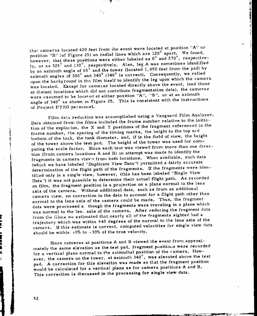
1
thai: cameras located 420 feet from the event were located at position "A" or
position "B" (of Figure 25)on radial lines which are 120° apart. We found,however, that these positions were either labeled as and 270 ° , respective-
ly, or as 325 ° and 130 °, respectively. Also, leg A was sometimes identified
by an azimuth angle of 65 ° and the tower (located 1,050 feet from the pad) by
azimuth angles of 300 ° and 340 ° (340 ° is correct). Consequently, we relied
upon the background in the film itself to identify the leg upon which the camerawas located. Except for cameras located directly above the event, (and those
at distant locations which did not contribute fragmentation data), the cameras
were assumed to be located at either position "A", "B", or at an azimuth
angle of 340 ° as shown in Figure 25. This is consistent with the instructions
of Project PYRO persGnnel.
Film da'_._ reduction was accomplished using a Vanguard Film Analyzer.
Data obtained from the films included the frame number relative to the initia-
tion of the explo.cion, the X and Y positions of the fragment referenced to the
frame number, the spacing of the timing marks, the height to the top and
bottom of the tank, the tank diameter, and, if in the field of view, the height
of the tower above the test pad. The height of the to_ver was used for com-
puting the scale factor. Since each test was viewed from more than one direc-tion (from camera locations A and B} an attempt was made to identify the
fragments in camera viev's from both locations. When available, such data
{which we have labeled "Duplicate View Data") permit-ted a fairly accuratedetermination of the flight path of the fragments. If the fragments were iden-
tified only in a single view, however, (this has been labeled "Single View
Data") it was not possible to determine their actual flight path. As recorded
on film, the fragment position is a projection on a plane normal to the lensaxis of the camera. Without additional data, such as from an additional
camera view, no correction to the data to account for a flight path other than
normal to the lens axis of the camera could be made. Thus, the fragment
data were processed a though the fragments were traveling in a plane whichwas normal to the len, axis of the camera. After reducing the fragment data
from tlm f_hns we estimated that nearly all of the fragments sighted had a
trajectory which was within ±45 degrees of the normal to the lens axis of thecamera. If this estimate is correct, computed velocities _or single view data
should be within +0% to -30% of the true velocity.
Since cameras at positions A and B viewed the event from approxi.
mately the same elevation as the test pad, fragment positioi_s were recorded
for a vertical plane normal to the azimuthal position of the ¢amera. How-
ever, the camera on the tower, at azimuth 340 ° , was elevated above the test
pad. A correction for this elevation was made so tl-at the fragment positionwould be calculated for a vertical plane as for camera positions A and B.
This correction is discussed in the processing for single view data.
5Z

<
L
2. Processing of Single View Data - As viewed from the camera, the
fireball and fragment would appear as in Figure 26 with the positive X axis to
the right and lying along ground surface and positive Y axis vertical throughthe center of the tank. Subscripts on the axes refer to the camera position
A or B from which the data are obtained. The view shown in Figure 26 is
typical of that obtained by a camera in position A. The angle between theintersection of the X-Y planes of cameras A and B is then 120 ° (this angle is
required for processing of the duplicate view data, but not for processing the
single view data). Fragment positions are measured on the film with re-
spect to the X and Y axes. Processed data are computed with respect to theX' and Y axes; that is, with respect to a set of axes which pass through the
center of the tank.
i
I'
The first items calculated from the film data are the film speed in
frames per second (fps), the scale factor (SF), and the height of the event
(he). Spacing of the timing marks (tin} are read from the film in frames pertiming mark. When spacing of timing marks is multiplied by the frequency
of the timing mark generator in timing marks per second, the framing rate
in frames per second is obtained. To compute the scale factor a known
length in the field of view is divided by its length as measured on the screen
of the Vanguard Analyzer. This give:-" the scale factor directly if the known
length is the same distance from the camera as the event; otherwise, an
appropriate adjustment must be made. The height of the event (h e ) can bedetermined from engineering drawings if they are available, but it is also
determined directly from the film data. It is computed as one-half the sum
of the distances to the top and to the bottom of the tank. Even though an
attempt was always made to align the X axis (Y = 0 position on the screen of
the Vanguard Analyzer) with the top of the pad, this alignment was never
exact. Consequently, whenever it is available, h e obtained from the filmmeasurement is used. t<nowing the film speed, the scale factor and the
height of the event, the X-Ypositions of the fragment can be calculated from
Equations (7) and (8).
xJ = x.j (SF) (7)1 1
]
YJ Yi (SF) _he (8)
cos 8 v 1 + dc sin _)v
Subscript i refers to the frame number and superscript j refers to the frag-ment number. Lower case x and y denote the values as read from the film,
and capital letters denote ca:culated displacements. The denominator of
Equation (8) is a correction factor which adjusts for the condition that the lens
optical axis may not be perpendicular to the vertical axis along which Y ia
53

YA
L
/.
SUCCESSIVE POSITIONS
___-_., .-_.. ,.TANK
FIGURE 26. FIREBALL AND FRAGMENT ._S VIEWED BY A
CAMERA LOCATED AT POSITION A
• l
54
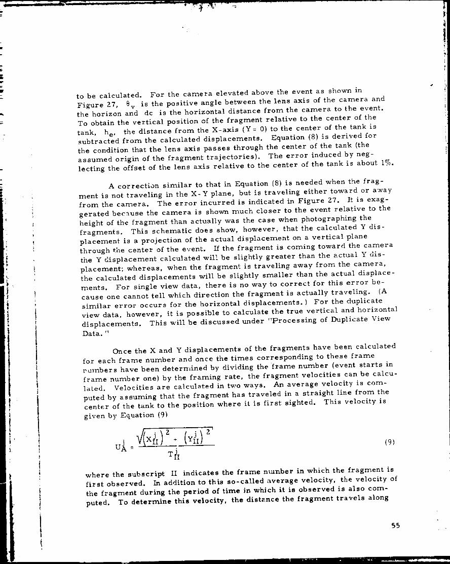
I
t
¢
to be calculated. For the camera elevated above the event as shown in
Figure 27, e v is the positive angle between the lens axis of the camera andthe horizon and dc is the horizontal distance from the camera to the event.
To obtain the vertical position of the fragment relative to the center of the
tank, h e , the distance from the X-axis (Y= 0) to the center of the tank issubtracted from the calculated displacements. Equation (8) is derived for
the condition that the lens axis passes through the center of the tank (the
assumed origin of the fragment trajectories). The error induced by neg-
lecting the offset of the lens axis relative to the center of the tank is about 1%.
A correction similar to that in Equation (8) is needed when the frag-
ment is not traveling in the X-Y plane, but is traveling either toward or away
from the camera. The error incurred is indicated in Figure 27. It is exag-
gerated because the camera is shown much closer to the event relative to the
height of the fragment than actually was the case when photographing the
fragments. This schematic does show, however, that the calculated Y dis-
placement is a projection of the actual displacement on a vertical plane
through the center of the event. If the fragment is coming toward the camera
the Y displacement calculated will be slightly greater than the actual Y dis-
placement; whereas, when the fragmen£ is traveling away from the camera,the calculated displacements will be slightly smaller than the actual displace-
ments. For single view data, there is no way to correct for this error be-
cause one cannot tell which direction the fragment is actually traveling. (A
similar error occurs for the horizontal displacements.) For the duplicate
view data, however, it is possible to calculate the true vertical and horizontal
displacements. This will be discussed under "Processing of Duplicate View
Data. "
Once the X and Y displacements of the fragments have been calculated
for each frame number and once the times corresponding to these frame
n_nbers have been detern_ined by dividing the frame number (event starts in
frame number one) by the framing rate, the fragment velocities can be calcu-
lated. Velocities are calculated in two ways. An average velocity is com-
puted by assuming that the fragment has traveled in a straight line from thecenter of the tank to the position where it is first sighted. This velocity is
given by Equation (9)
{9)
indicates the frame ntunber in which the fragment iswhere the subscript IIfirst observed. In addition to this so-called average velocity, the velocity of
the fragment during the period of time in which it is observed is also com-
puted. To determine this velocity, the distance the fragment travels along
55
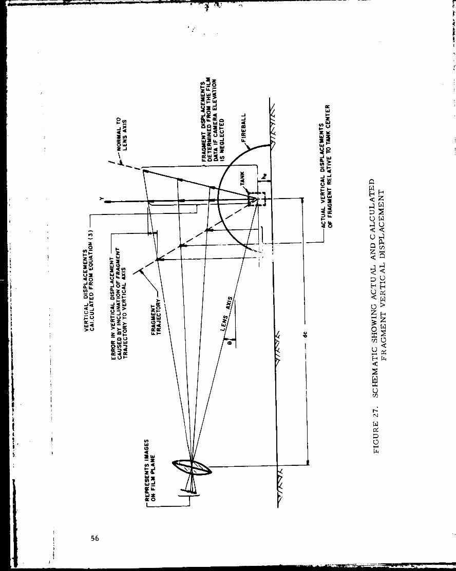
.i
iIi
i'
T
!
<Z
L3_
<<
Z_
<N
Z_
M
L)
56
I
?
77
0
|
its trajectory after first being sighted is calculated from Equations (10)
and (1 l)
(10)
1-1 1
where the distance S is set to 0 at the time of sighting. Velocity of the frag-
ment, U i, is then determined from the slope of a straight line fit to the com-
puted distance-time data points S i and T i, where T i is adjusted to 0 atthe time of sighting as was Si. The subscript i on the velocity is used to
denote an instantaneous velocity. While it is true that this velocity is actually
an average over the time of sighting, the elapsed time is short compared to
the elapsed time between the explosion and the sighting of the fragment for
which U A was determined and the velocity of the fragment varies only slight-
ly during the time of sighting. Also, the position of the fragment which corre-
sponds to U i is computed for the center of range over which the fragment is
tracked (as discussed below} and U i should be very close to the instantaneous
velocity at this position.
In addition to the fragment velocities, the position of the fragment
relative to the center of the event and its direction of travel are computed.
Fragment coordinates are given as a radius R, height _, and an azimuth
angle _. Since the computed velocity, U i, is taken to be the instantaneousvelocity of the fragment at the center of its range of travel while in view. _-_._
cylindrical coordinates are computed for this position also. The expressions
for determining these coordinates are
t ) <13>J
_J xIF (90) + 'fc (14)
IF _J < 0.0 set _/'J : 360 + _J (15)
where the subscript IF denotes the final frame in which the position of the
fragment _as recorded. Notice that R and _ are simply the center posi-tion of the " xnge of the X and Y coordinates, respectively. The azinouth
57
i°
position i_ determined from the azimuth angle, _c, of the camera viewingthe fragment and the sign of the X displacement. This is based on the assump-
tion that the fragment is traveling in the X-Y plane which is normal to the line
of sight of the camera. (For fragments which are photographed, and properlyidentified from two different camera positions, the azimuth angle of the line
of flight can be determined more exactly. ) The last parameter computed for
the fragment is the elevation angle of its flight path above the horizon. This
angle, e, as shown in Figure 26, is determined from the slope of a straight
line fit to the X-Y data for each fragment.
3. Processing of Duplicate View Data - After the single view data for
each fragment had been processed, data for those fragments which could beidentified in more than one camera view, that is, in views from camera posi-
tions A and B of Figure 25, were combined to more accurately determine a
true trajectory of the fragments. Fragments were difficult to identify in morethan one view, however, and thus the duplicate view data are very limited.
In addition, we have otten found when processing the data that what appeared
to be the same fragment in two separate views, apparently was not. One cri-
terion for determining whether or not the fragment is the same in two views
are the Y (displacements. They should be approximately the same when view-
ed from the two camera positions. As noted in Figure 27, there will be some
differences depending on whether the fragment is traveling toward or a_'ay
from the camera; however, these differences should be small because the
cameras are located 420 feet from the event and it is unusual to follow a frag-
ment for a distance of more than 60 feet above the ground. Thus, the cameras
are viewing the fragment at .an angle of less than 10 ° above the horizon. Al-
though no hard and fast rule was established, when the Y displacements of the
two fragments differed by more than about 15%, it was assumed that two dif-
ferent :_ragments rather than the same fragment had been observed.
In duplicate view data, the same fragment is observed from cameras
situated 120 ° apart. Thus, errors introducc_by the fragment traveling
toward or away from the camera tend to cancel out when averaging the Y dis-
placements computed from the two different camera views. Consequently,the vertical displacements, 6, are calculated as the average of the vertical
displacements from the single view data. This is shown in Equation (16)
i6 =
JY + y UP (16)
where the superscript DUP is the number of the fragment ,vhlch provides
the additional camera view of fragment "j".
Calculating the horizontal position of the fragment is more complicated.
Figure 28 shows the geometry in plan view. The X displacements of the frag-
ment, computed from the two separate camera views, are indicated by X A
58
:/
l
FRAGMENTPOSITRON
/
_P'POSI T ION A
0 °
dc A
EVENT
240 °
dc B \
POSITION B
240 °
FIGURE 2.8.GEOMETRY FOR FRAGMENT POSITION FORDUPLICATE VIEWS
_9

r
i
i
!
and X B. These are projections of the fragment horizontal displacement upon
the X-Y planes for each camera position. The true horizontal displacement of
the fragment, H F. relative to the center of the event is desired. Using
si,nple geometrical relationships, two expressions for H F were obtained and
are given by Equations (17) and (18)
XA deA (17)
HF = X A cosa + dc A sin_ for X A _ 0
-XB dCB for X B _ 0H F = XB cos(A0_+c_) + dc B sin(60°+R)
(18)
$_s indicated, Equation (17) cannot be used for X A = 0 and Equation (18)
c_nnot be used for X B = 0. In practice, Equation (17) was used whenever the
absolute value of X A was greater than X B, and Equation (181 was used when
the reve.'se was true. Subscript i and superscript j have been dropped
from the equations for simplicity. The angle, _, is found by equating Equations
(I:')to (I8}, and is given by Equation (19}.
cl : tan"l XAXB c°s60°+ XAXB dcB/dCA + XA dcB sinb0C
XAX B sin 60 _ XB dc B - X A dc B cos 60 °(19)
Equations (17), (18), and (19) hold for fragment positions in all quadrants.
The sa:,_e procedures were used in calculating the average velocity,
UA, and the velocity of the fragment after acquisition, U i, as were used
for the single view data. Quantities U and H were simply substituted for
X anl Y. Also, with the exception of the azimuth angle, the cylindrical
coorcinates of the fragment and the elevation argle _) wer_ computed as for
the single view data. The azimuth position of the fragment is simply 360 c
minus the angle _.
4. Computer Program for Data Processing - A computer program was
writtez_ to process the data as it was received in punched card t,_rrrt from the
Vanguard Analyzer. Although the details of the program will not be presentedhere. it solves the e¢"a }ns given in the preceding sections and prints the
results in a usable form. The program also creates a tape file for subsequent
statisti:a] analysis of the results.
A s,_mmary of camera data and number of fragments whose trajectories
were _,,asure_ is given in Appendix A. The tests are grouped by, type, as
defined in the PYRO reports (refs. 15 through 17}, and are identified by the
PYRO test numbers, Numbers of fragments whose velocities and trajectories
60
<
!r
were measured range from a minimum of 2 per test to a maximum of 36 per
test. The maximum number of fragments identified in duplicate views was
3 per test.
5. Summary of Fragment Velocity Measurements and Calculations -
The fragment velocity data derived from the PYRO films are available on
punched cards and in computer printouts. The key designator for all data isthe PYRO test number; for each such test having readable fragment velocity
data, all of the quantities defined by the equations in Section 4 are calculated
and printed for each fragment traced. The printouts are quite voluminous
and so are not included in this report.
The data for each test were further reduced using standard statistical
procedures and a " anned" computer program available to us through our_CDC
library of programs. We chose the six output variables U A, U i, 8, %, R,
and H F for statistical treatment, and computed the mean, standard devia-tion, standard error of the mean, maximum, minimum, and range for each
variable, Again, the computer printout sheets are too detailed for inclusion
in the report, but are available for study.
A summary of results is given in Table V. Each test is identified by
the PYRO test number, and the tests are grouped by propellant and type of
simulated accident. Test conditions given are total weight of propellant,
tank L/D ratio, and impact or drop velocity. Ignition time and measured
blast yield from reference 16 are listed. _" Fragmentation data are given in
the last four columns, indicating nurrAber of camera views from which data
were taken, number of fragments observed, mean value of fragment velocity,
Ui, and standard deviation of this same parameter o u. "i'hese mean velocitiesand standard deviations were determined from the single view data only. The
number of fragments _vhich were identified in more than one camera view and
processed as duplicate view data was too small for statistical analysis. Be-
cause the data represent a wide spectrum of test conditions, propellant types,
and propellant weights, they should allow correlation with methods of pre-
diction of initial velocity such as those presented later in this section, and
Should also lend themselves to various types of statistical analysis. A limi-
tation to the data which may render statistical studies difficult is that rela.
tiveIy few fragments could be observed in any one test. Some grouping be-
tween tests with different propellants, different blast yields, etc. , may be
possible. To aid in rational choice of ways to group the test results, we con-
ducted several limited model studies. The-e are included in this report as
Appendix C.
Blast yield in percent iA delined in Section lI.
61
i
t
!,i
6Z
L_
Z
<
p+
,-3
Z
<c_
0
:m
>
oE.
_0
c_
0__0_
__00
A
<
0
***o..I
0IIIllll
IIIIIIII
IIIIIII
I I I I I I I
I I I I I I I
NNNN_'NNO
_J
,J
!
I
>.
!
Z
ZEZ0
"T
N0,-1
..
;3
0
G
O_ 0000_ N_ _
IIIIIIIIII
IIIIIIiiii
|llillllll
0000000000_ 000000000NNNNNNOO_N
i.
.m
P_
oE I
Zu
o_u
.,,,IN_NI
II_IIII IIIIIII
I
A00000
- 0000000000
NNN_U
0
CO
_q
<
o<
I
C_Z
0
|
I
Z0
N
0,-1
o
NNNNNNNN _NN
00000000000000000000_0NffJoON_3NOONO
OO_ O ___NNNNNNN
U3
U3
[.-,
ON
0
<
I
c_
0
i
I
E_Z
,,,-¢ f_.l ,-_ N N
_N_NN
N
IIIIII
Z ,,,,,,0
I
__ 0N __
O
0 oooooo000000
>
0
o
..._
63

0
"0,-i
0.,.4 _)
__ __ _N_ _N
I
I
Z0u
N
N
0
°,
D-
0
O
NNNNN_N_r_NNNNNNNN_
NNONOO ONNNON NN__
_ _ _ I _ _ I _O 000_
__'
I Illlllllllll_ IIIlllill,llllllllll IIIIIIiiiiiiIIIl_tlllllllll
0000000000000_0000000
0000000000000_0000000
NNN_NNNNNNNNN_NN_ _OOO
N
U_
U3
,J.<
u
u<
U_
Z
0
0I
I
m
Z
z0 _
0oooo
0 ooooN_N_
¢
E _, p..,..
"-' ----
.J
f-.,
_ _ _ _ _ N_ _ _ _
NNNNNNNN_N_ N__
NQNNNNNNNNNNOOQNN
N_
O0 _p ,.. 0., 0 N .._ 0 0,, O0 _' 0 ,,D ,,O 0 _O0 Ntl'_ _'_ e_ I _r t_,l N I fe_ '''_ '='_ I I
I
A"0
4.1
0
v
o_
0
0
OOOOOOO OOOOOOOOOCOOOOOOOOOOOOOOOO_NNNNNN_IOONNOOOOOO
f_N_
,.._,._,.._,.._,.., N_INN|'|NNNNNN N
NN_N_
<
Z0N
0 __N
<
_NNNN
0NNNNN
0 ooooo!
I
N
N
0
_N_
0
0 ooooo00000
U
U0
Q;
>
0
0
>
b5
•1. _
|
I_,.w
L)
£_ °,4
4-*
¢g
u_[.-,vJ
,-]
,-, O0 ,q'_
0" t"- _unO un
e,,] N N
t.,...o ,_1_
_o
L_
_:_ _,_a-..,o
0 _ _
0
0_ e!_ _NN
O0 0O0 0
¢_1N m
ta
o_
g,
0
0
m 0O
N e_
00 Cr_
er_
N
_1_ N
_D
0I u_
!
o oO O
N
._p ur_Cr_ 0 _
,.0
,,C
Z
U3
_D
!
II
_D
e_CO
II
I
¢)¢3o
0,
P,I
0
m
N
0
U
.%0
o

C. Methods of Predicting Velocity
1. Explosions Within Missile Tanks
a. A Deterministic Method
( 1 ) Choice of Parameter s and Idealization of the Problem -
In this section, we discuss a method for predicting maximum velocities for
fragments generated by explosions within missile tankage (CBM case). A
method for predicting ranges is discussed in Section IV. In order to predict
maximum fragment velocities, the problem must be "idealized" in a number
of ways, and the parameters must be chosen such that the theory may be
applicable to a spectrum of missile explosions involving different liquid fuelsand oxidizers, volume of fuel oxidizer mixtures, tank wail specific mass; and
tank geometries. To idealize the problem we consider only a spherical
volume Voo of radius R o in which we have a stoichiometric mixture of thatamount of fuel and oxidizer which is mixed at time of detonation. Further-
more, upon detonation, all of this volume of fuel and oxidizer is assumed to
be converted instantly to explosive products and energy, forming a "hot gas"
which can be characterized by some ratio of specific heats. _, initial pres-
sure, Poo, and initial sound velocity aoo. All of the fuel or oxidizer ex-
ternal to this spherical volume is considered to add mass to the container
wall only and sakes no part in the chemical reaction of the explosive process.
The container is spherically coincentric to the sphere in which the explosion
takes place, and the non-reacting fuel (or oxidizer) moves initially with the
fragments of this container wall as if they were an integral part of the frag-
ments (i.e., they just add mass to these fragments). Compression of the
liquid fuel and oxidizer, and shock transmission effects in these liquids are
ignored.
All fragments are assumed of equal size and have circular projections.
If we pick a parameter, n, for the number of such fragments into which the
containing sphere fractures, we can later solve the problem for various n,
thus effectively varying the fragment size. It is further assumed that the sum
of the concave inner surface areas of all the fragments is equal to the surface
area of the original sphere of explosion.
A i = 4 v R2/n (20)
[R_ r i (_) T :_0],where R i_ the initial radius of the sphere of explosion for
and A i is the fragment surface area, Although these are gross idealiza-
tions of the fragmentation picture, they make tbe problem amenable to solu-
tion and allow some estimate to be made of how sensitive the solution is to
fragment size and number.
67
_°_
If the stoichionaetric mixture of fuel and oxidizer occupies a volume
V o and has a mass M o, then, at the time T = 0 the instant after the ex-
plosion, we assume the gaseous products of explosion occupy the same
volume and have the same mass. The sound speed in this medium at this
time is then a function of a, one of the independent parameters. One n_ust
pick k, Moo, Vo(0), and Po(0) = Poo which characterize the sphere of
explosion at T = 0 (_, M o, and Poo will depend on the type of fuel and oxi-
dizer, and V o depends on the amount of fuel and oxidizer that have mixed}.
One must then also pick an R, n, and M t which characterize the con-
taining sphere (where R is tlle containing sphere's initial internal radius,
equal to the external radius of the sphere of explosion; n is the number of
fragments into which the containing sphere fragments, and M t is the total
mass of the containing sphere, i.e., the mass of the non-reactants, as well
as the actual fuel tank mass). With this information the maximum fragment
velocity for any of the equal sized n fragments is calculated : : the method
to be described. This maximum velocity, U m, may be used as the initial
fragment velocity for the fragment range calculation (Section IV) in which the
fragment is assumed to experience no acceleration due to the explosion after
U m is attained, but it experiences deceleration due to drag forces in the
medium through which it is traveling.
(2) Equations for the Mathematical Model*- To obtain
the initial velocities for the fragments from CBM explosions, an extension
was made of the techniques of D. ]_. Taylor and C. F. Price (ref. 31) and of
G. L. Grodzonski and F. A. Kukanov (ref. 32) relating to the motion of frag-
ments from bursting gas reservoirs in a vacuum. These techniques were
generalized from the case of spherical vessels which broke up into two per-
fectly hemispherical fragments to the case of a spherical vessel which frag-
ments into n fragments, each of equal size and having a circular projection.
For the case where the containing sphere is thin-walled, the equation of
motion for the i-th fragment of mass M i and radial displacement ri(T)
having a projected area F and experiencing a pressure Pi(7) at time T, is
given by:
d 2 ri(T_:- F Pi(T) (21)
Mi d_2
If A i is the area of the curved surface of the spherical segment (for the i-th
fragment}, then
:::The equations given in this section require a number of mathematical opera-
tions for their development. Many of these operations are omitted for
brevity. All nomenclature is given in Appendix I.
68

A i : 2v_ Rh : 4_ R2/n (22)
where R = ri(0) and h is the segment height. Let the segment radius equal
d/2, then it can be shown with the use of Equation (22) that
4 o
or
F _ A i for n 2 >> n (23b)
The equation of state assumed for the gaseous products of explosion is given by
Po(_) V o(T) : c(_) R 1 T o(T) (24)
The rate of change in the mass of the confined gaseous explosion products in
the sphere as the sphere begins to fragment and gas is lost to the external
sphere region is given by
dc(q') _ -k P.,.a, _ w (25)dT ..... '
where P.,. and a.,= are the critical gas density and velocity as they escapethrough t'[ae cracked surface of the sphere, [i is the crack perimeter, w is
the crack width, and k is a discharge coefficient. The crack area for the
i-th fragment given by (I_ w)i is equal to the difference betwcen the area sub-
tended by the initial solid angle, ¢, at the distance ri(_) for time T and
the actual area of the fragment A i.
R 2 ( r2(T)4vT (26)
Inherent in Equation (26) is the assumption that all fragments travel in a radial
direction and that the synametry of the fragment motion i3 such that the equa-
tions of motion are only a function of the magnitude of the radius, i.e., the
motion of the i-th fragment in the radial direction describes the motion of
any other fragment in the radial direction and shear forces are small com-
pared to dynamic forces. Thus, we may set r i : r and, from Equations (25)
and (26), we have
\R 2
:: -k O::.a, lJ.4rr
,,'- \ R2
(27)
69
)'
j,
The volume of the gaseous explosion products at any time T after
T = 0 is given by
Vo(_) = (4/31u r3(T) (28)
It has been assumed that the confined gas immediately adjacent to the
fragments is accelerated to the velocity of the fragments but that this con-
stitutes a negligible fraction of the gas, the great bulk of which is unaccel-
erated. Thus, from one-dimensional flow equations
Pi(T) = Po(T) [I - ( ., 12(ao(T))z \_7-_ /
_/(),.- l)(29a)
P;::= Po(T)(_____.] II()4-I)
(29b)
/ 2 ) 1/2a::.--ao(T)\-/T]'+I(29c)
Equations (29) can be non-dimensionalized by setting
r(T) Xg(_) T = O _ Po(T) = Poo P, (<--)(30)
For a confined gas that behaves adiabatically we have:
= _ (3i)-- \-T-77-ooi
where the double zero subscripts refer to the confined gas condition at T = 0.
From Equations (20), (29), (30), and (31), one obtains:
Mi. [ (g')2 ] x/(x-1)M_ g P_. l (p,::) (x- l)/x
where primes denote derivatives with respect to _, Mi is the mass of
the i-th fragment, and M t is the total "shell" mass. For n fragments of
equal size,
Mi 1 (33)
M t n
7O

thu s,
g :nP [1-](p,)( )/'_
x/(×-l)(34)
!
where
I_) _aooa°° 0 -X = -- _ , F Poo
F Poo
Differentiating Equation (31) and nondimensionalizing,
where
<el ]_(n) = R6W 2 Mt 2 aoo4 n'2
(2_____y)1/2
one obtains
2
(35)
(36)
and
Equations (35) and (36) must be solved simultaneously with the initial
conditions
r(o) : R .'. g(o) : R/X
( ) " P (o): 1Po o = Poo " • *
for values of _ until the fragment acceleration is small with respect to the
acceleration -t T = 0. dg/d_ is a maximum as the acceleration goes to
zero. dg/d_ is the normalized initial velocity for the fragments to be used
in the calculation of the fragment ranges.
!
i
!
(3) Solution of the Equations by Numerical Techniques
and Computer Program - The solutlon of Equa-
tions (34) and (36) may be obtained numerically for the initial conditions of
Equations (37), using the Runge-Kutta method. A program which does this
(in FORTRAN IV), as well as the definition of its symbols, is given in
Appendix C. This program requires as input the characteristics of the gas-
eous explosion products at _ -- 0 (A¢, the speed of sound; PC,, the initial
pressure; and CAP1, the ratio of specific heats), and the cbaracteristics of
the vessel (R]Z, the internal radius of vessel and unburned fuel; TM, the mass
of the vessel and unburned fuel; and FN, the number of fragments). Also, a
guess must be made on the elapsed time between detonation and zero fragment
acceleration, XMAX.* A time interval spacing, AH, must also be chosen
for the calculation.
The program outputs the normalized displacement, velocity and accel-
eration (dynamic variables) of the fragment as a function of time; the normal-
ized pressure within the vessel as a function of time; and the final values of
time, displacement, velocity, acceleration, and pressure at XMAX. A
sample program run is given in Appendix C.
Figure 29 shows the results for computing the maximum fragment
velocity as a function of number of fragments when all other parameters are
held constant. The figure indicates that the number of fragments does not
affect maximum fragment velocity except at very low a (at which point the
assumption of Equation (23b) does not hold). Figure 30 shows how maximum
fragment velocity varies with n and the mass ratio Mo/M t. The ratio of
explosive products mass to shell and non-reactant fuel mass, a constant
initial pressure (Poo), number of fragments (n), sound velocity (ao), a,d
radius of explosion at T = 0 (R) are assumed in this figure.
(4) Comparison of Results from this Method withOther Sources - The results of this method are
compared to the cases described by Taylor and Price (ref. 31) in which:
PoVoC_ _ - 2.55, O. 1436
1Vitao 2
r::
A "guess" is made of XMAX because the computer has to work with so.ne
finite time. If XMAX is guessed too short, then g"(_) (the normalized
acceleration) is not reduced close enough to zero to yield an acceptable
'(estimate of g _). if XMAX is guessed too long then the computer can nota i t
calculate the final values of g and g . In practice we watched g for
each program iteration and accepted a g' which remained constant to three
significant figures between iterations as the value of g for g nearly zero.
72

3es/_,t'tuff AII30I]A JN3WOV'd.-IWFIWIXVW
k40
Z0
Z
<
<
8r't
_ZZ N
©<
_z
?3
_ " 11 _
74
p,_ I,--I
_Sl. 'wN _I3)'I]A ll_WgY_IdWNWIXVW
Ni,,-d
J
N
0
(._ L,.:
'_.
_'_,..,<
_ m
t3
_0 au
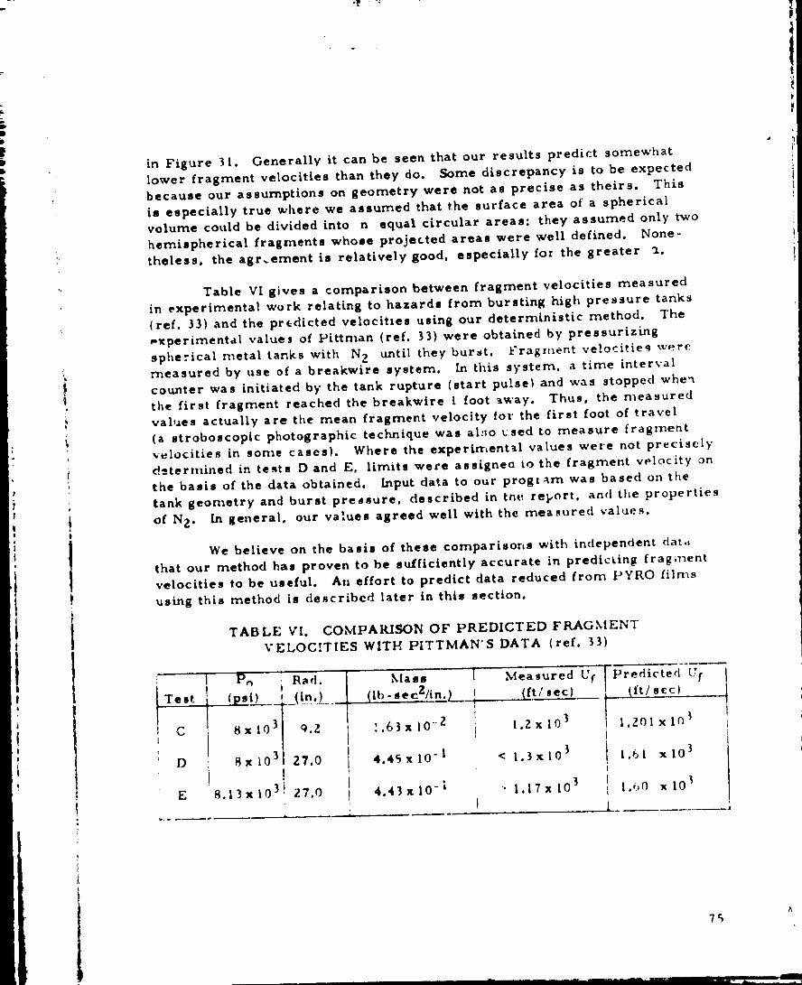
in Figure 31. Generally it can be seen that our results predict somewhatlower fragment velocities than they do. Some discrepancy is to be expected
because our assumptions on geometry were not as precise as theirs. This
is especially true where we assumed that the surface area of a spherical
volume could be divided into n equal circular areas; they assumed only two
hemispherical frag:nents whose projected areas were well defined. None-
theless, the agr.ernent is relatively good, especially for the greater _t.
Table V[ gives a comparison between fragment velocities measured
in experimental work relating to hazards from bursting high pressure tanks
{ref. 33) and the predicted velocities using our deterministic method. "['he
_.xperimental values of Pittman {ref. 33) were obtained by pressurizing
spherical metal tanks with N 2 until they burst. Fragzzxent velocities werer_easured by use of a breakwire system. _ this system, a time interval
counter was initiated by the tank rupture (start pulse_ and was stopped whe'_
the first fragment reached the breakwire [ foot _way. Thus, the measured
values actually are the mean fragment velocity tot the first foot of travel
{a stroboscopic photographic technique was al:lo _sed to measure fragment
velocities in some cases). Where the experimental values were not precisely
d_termined in tents Dand E, limits were assigneo to the fragment velocity on
the basis of the data obtained. Input data to our progzarn was based on the
tank geometry and burst pressure, described in the rel_ort, and the properties
of N Z. In general, our valueA agreed well with the measured values.
We believe on the basis of these comparisons with independent datd
that our method has proven to be sufficiently accurate in predicting frag_ent
velocities to be useful. All effort to predict data reduced from PYRO filn_s
using this method is describcd later in this section.
TABLE VI. COMPARISON OF PREDICTED FKAGMENT
VELOCITIES WITH PITTMAN'S DATA {ref. 33)
Test
C
D
E
Pf_
(psi_) ....
8xlO 3
, 8xiO 3
8.13x10 3
R_d. 1 Mass 1{l 'se Z/in'LI
9.2 I..63 x I0'2 i
4.45 x lO- !27.0
27.0
h i, ,
4.43x I0 -i
Measured Uf
(ft/sec)
l.Z x iO 3
< 1.3xl03
• 1.17 x 10³
Predicted (If
_t't/scc)
1.201 x I_ _
1.61 x I0 _
I._:,0x I0 _
7_
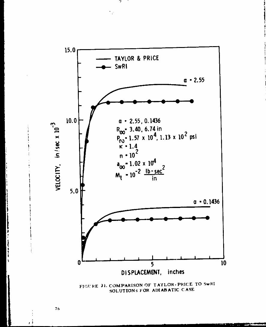
I
15.0
I0.0
0
FIGI"/_ E
TAYLOR & PRICE
SwRI
a - 2.55
a • 2.55, 0.1436
Roo- 3.40, 6.74 in
Poo"1.57 x 10⁴, 1.13 x 10² psiK-I.4
n - 102
aoo" 1"02 x 104 2-2 Ib-sec
Mt - I0 in
a • 0.1436
5
DI SPLACEMENT, inches
31. COMPARISON OF TAYLOR-PRICE TO SwRl
SOLUT|ON_ FOR ADIABATIC CASE
l0
7h
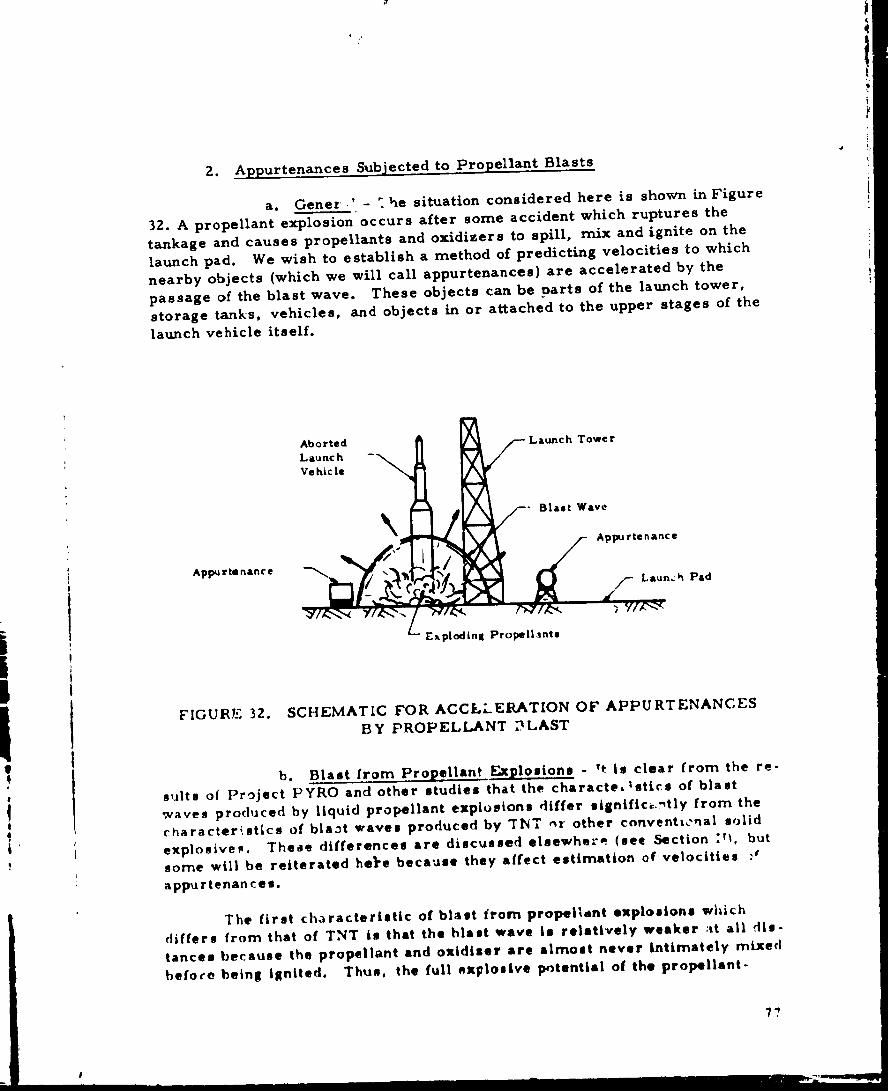
2. Appurtenances Subjected to Propellant Blasts
a. Gener ' - _-he situation considered here is shown in Figure
32. A propellant explosion occurs after some accident which ruptures the
tankage and causes propellants and oxidizers to spill, mix and ignite on the
launch pad. We wish to establish a method of predicting velocities to which
nearby objects (which we will call appurtenances) are accelerated by the
passage of the blast wave. These objects can be Darts of the launch tower,
storage tanks, vehicles, and objects in or attached to the upper stages of the
launch vehicle itself.
,i
i
ApI_ rte nan¢ •
Launch -
Ve hic le
_'" /- Appurtenance
Explod_n I Prope|lznte
FIGURI£ 32. SCHEMATIC FOR ACC_-LER ATION OF APPURTENANCES
BY PROPELLANT _LAST
b. Blast from Propellant. Explosions - 't is clear from the re-
sults of Project PYRO and other studies that the characte,'stlcs of blast
waves produced by liquid propellant explosions differ signifi¢_.ntly from the
character;.stics of blazt waves produced by TI_T ,_r other conventlenal solid
explosive_. The_e differences are discussed elsewhere (see Section :T_, but
some will be reiterated he_'e because they affect estimation of velocities :¢
appurtenances.
The first characterlstic of blast from propellant explosions which
differs from that of TNT is that the blast wave is relatively weaker _t all dis-
tances because the propellant and oxidiser are almost never intimately mixed
hefoce being ignited. Thus, the full explosive potential of the propellant-
77
r
r
i
tiL •
oxidizer computed on the basis of energy of combustion is never realized.
This difference is expressed, when comparing with blast waves from TNT
explosions, as a percentage or fraction of ttTNT yield", where the per-
centage must be multiplied by the total weight of propellant plus oxidizer,
and then expresses the weight of TNT which will produce the same blast pro-
perties far enough from the explosion source.
The second characteristic of the blast from propellant explosions which
differs from the blast from TNT explosions is that measured parameters such
as peak overpressure and positive phase impulse vary with range in a different
manner. Compared to TNT blasts, equal energy propellant explosions gener-
ate blas _- waves with relatively low overpressures and relatively high im-
pulses {longer durations) at close-in distances, with gradual change to nearly
identical pressures and impulses with increasing range. Below about 10 psi
overpressure, blast characteristics from the two types of sources appear to
be essentially identical. The term "terminal yield" has been introduced to
designate blast yield calculated from measured blast parameters in the low-
pressure regime. The basis for estimating the terminal yield is usually a
source of compiled blast clatafor hemispherical TNT charges detonated on
the ground (see ref. Z).
A third facet of difference between TNT explosions and liquid propellant
explosions can seriously affect c)ur ability to predict fragment velocities of
appurtenances. For TINT explosions, there are available both a quantity of
measuren_ents of time histories of dynamic pressures, and also proven co_z_-
purer programs which c_n predict time histories of this and other physical
properties of blast waves. For liquid propellant explosions, the only com-
plete body of data available is for time histories of overpressure, from Pro-
ject PYRO (refs. 15 through 17). Methods are presented in Section !l for esti-rnation of certain blast wave properties for several propellant combinations in
test configurations which simulate accidental spill and subsequent ignition
{identified in Section II as CBGS - Confined By the Ground Surfacel. The
parameters which can be estimated, given type of propellant, total weight of
propellant W t, impact velocity U[, time of ignition t, and distance B from
the center of the explosion to an appurtenance, are the side-on peak overpres-stirs P and the side-on impulse I. As we see later, these values must be
used together with other data to estimate the pressures exerted on a body as
,he blast wave diffracts around it.
c. lntGraction of Blast Waves with Appurtenances - To be able
to pr;dict velocities to which apl_Irtenances are accelerated by propellant
blasts, we must know something about the physics of interaction of blast waves
with solid ,,bjects. Some of this knowled|e is briefly reviewed here. Figure
33 show,J schematically, in three stages, the interaction of a blast wave with
an i.--re|_Har object. As the wave strikes the object, a portion is reflected(ronathe front (ace, and the remainder diffracts around the object. In the
78

®
FIGURE 33. INTEKACTION OF BLAST WAVE WITH
IRREGULAR OBJECT.
diffraction process, the incident wave front closes in behind the object, great-
ly weakened locally, and a pair of trailing vortices is formed. Rarefactionwaves sweep across the front face, attenuating the initial reflected blast pres-
sure. After passage of the front, the body is immersed in a time-varying
flow field. Maximum pressure on the front face during this "drag" phase of
loading is the stagnation pressure.
We are interested in the net transverse pressure on the object as a
function of time. This loading, somewhat idealized, is shown in Figure 34.
(Details on calculation are given in The Effects o! Nuclear Weapol_s, ref. 34. }At time of arrival t a, the net tratteverse pressure rises linearly from zero
to maximum of Pr in time (T l -t a) (for a fiat-faced object, this time iszero}, lh'essure then falls linearly to drag pressure in time (T Z . TI} , and
then decays mnre slowly to zero in time (T 3 - TZ). The time history of drag
press_ire is a modified exponential, with maximum given by
Z _38tC D Q C D • t 0s Us
where C D is the steady-state drag coefficient for the object. O is pe_kdynamic pressure, and _s and u s are peak density an# particle velocity re-
spectively for t!,e blast wave. The characteristics of the diffraction phase of
the loading can be determined easily if the peak slde-on overpressure F s or
the shocL ,--iocity U are known, together with the shape and some char_ c-
teristlc dlmensi<,.. D of the object. The peak amplitude of the drag phase.
CL-)Q, can also be de,ermined explicitly from Ps or u s. Bu___t, the time
,.Q
.eq__d_. _
l_e sStlYe
Pr
CDQ JJ __it
a
T 1
_D 1 Z
= •
T3 TimeT Z
FIGURE 34. TIME HISTORY OF NET TRANSVERSE PRESSURE ON
OBJECT DURING PASSAGE OF A BLAST WAVE
history of the ensuing drag loading, C D q(t), is quite difficult to predict
accurately for propellant blasts.
d. Method of Estimating Net Transverse Pressure - The
method we present here utilizes the fits of Section II to PYRO data for side-on
blast p_rameters, an assumed time history of drag pressure known to be rea-
sonably accurate for TNT and nuclear blasts, estimates of diffraction times
based on shock tube experiments, drag coefficients from wind tunnel data, and
reflected and stagnation blast front properties based on equations which are
well known in blast physics.
Side-on overpressure is often expressed as a function of time by the
modified Friedlander equation (see Chapter I of ref. l).
-bt/T (39)p (t) : P (| - t/T} •
where T is the duration of the positive phase of the blast wave. Integrating
this equation give_ the impulse
T
I = f p(ti dt
o
The dimensionless parameter b is called the time constant,
shock stren|th, and is reported in Chapter 6 of ref. I.ica|ly in Fi|,tfe 35 (or s range of shock siren|the _;,
(40)
is a function of
It is plotted graph-where
gO
J
,4
i
!,!
I \
\\\
J_
\ !
0
/Q
0
u3
,..JZ0
Zal
Z_O_
a2o
;>
m
C
L/,
P = P/Po(41)
and Po is ambient air pressure. The peak reflected overpressure Pr and
peak dynamic pressure Q are unique functions of P for a given ambient
pressure Po" For shocks of intermediate to weak strengths, P <__ 3.5, these
functions are (see ref. 1, Chapter 0):
2 (4z)Pr = 2P _ 4
and
5 P_ (43)
3 7,P
where
Pr = Pr/Po ' Q = Q/Po (44)
For the time history of drag pressure, a good fitto experimental data for TNT
is a slightly modified form of that employed by Glasstone (ref. 34),
q(t) : Q {l -t/T) 2 e"bt/T (45)
The procedure for determining the transverse loading blast parameters in
Figure 34 which are independent of object size and shape is then as follows:
(l) Obtain P and I from curves in Section II
(2) Calculate P
(3) Bead b from Figure 35
(,i) Solve Equation (40)for T. knowing P, I, and b
(5) Substitute P in Equations (42) and (43) to _btain
(6! Obtain Pr and Q from Equation (44_
(7} Substitute in Equation (45) for q(t), realizing that T - 3 3 - t a
in Figure 34.
Pr and O
The remaining quantities needed to define thL time history of trans-
verse pressure are dependent on the size and shape of the object. They are
only well defined for objects of regular shape, such as right circular cylinders.
flat rectangul_r strips, etc. Methods for estimatinl[ (T 1 -t a) and (T Z- T l)
are given by Glasstone (ref. 34_ for several such objects, and will not be re-
peated here. One does need to know, however, the shock front velocity U.
)i
iI
i
This is a unique function of the shock strength _, and is given by (see
Chapter 6 of ref. 1)
6 P (4651 + --y-
Drag coefficients C D are available from Hoerner (ref. 355 for a variety ofbodies over a wide range of flow velocities. Estimates for the subsonic flow
range which applies over the shock strengths of interest to us are given inTable Vii. Melding these quantities, dependent on the size and shape of the
body, to the previous ones which are derivable from side-on blast wave pro-
perties permits an estimate of the entire time history of transverse pressure,
at least for bodies of regular geometry.
e. Method of Predicting Appurtenance Velocity - Once the time
history of net transverse pressure loading is known, the prediction of appur-tenance velocity can be made quite easily. The basic assumptions are that the
appurtenance behaves as a rigid body, that none of the energy in the blast waveis absorbed in breaking the appurtenance loose from its moorings or deform-
ing elastically or plastically, and that gravity effects can be ignored duringthis acceleration phase of the motion. The equation of motion of the object is
then
Ap(t} = M_ (47)
where A is the area of the object presented to the blast front, p(t) is the
net transverse pressure accoJdingto Figure 34, M is the total mass of the
object, and x is displacement of the object (dots denote derivatives with re-
spect to time}. The object is assumed to be at re_t initially, so that
x (o5 : 0, i (o5 = 0 (481
Eq,lation (47) can be integrated directly. With use of the initial conditions
(485, this operation yields, for appurtenance velocity,
(T3-t a )
A _ A ldx(t) = _ p_t) dt -0
(49)
where Id is total drag and diffraction impulse. The integrations in Equation(4q) can be pe_formed explicitly if the preslure time history is described by
suitable mathematical functions, or performed graphically or numerically if
p(t) cannot be easily written in function form. In either caws, Equation (49)
yields the desired result--a predicted velocity for the object.
83

TABLE VII
DRAG COEFFICIENTS, C D, OF VARIOUS SHAPES
Source: ref. 35)
SHAPE
Right Circular Cylinder
(long rod), side-on
Sphe re
SKETCH
nl
_od, end-on
Disc. face-on
Cube, face-on
Cube, edge-on
Long Rectangular Member
face-on
Lonk Rectangular Member,
@dge-on
Narrow Strip. [ace-cMn
or _ .L
C D
I. Z0
O. 47
O. 8Z
1.17
1.05
0.80
Z. 05
1.55
84
D. Correlation of Velocity Prediction Methods With Data
1. Prediction of PYRO Data by a Deterministic Method for CBM - A
deterministic method of predicting initial fragment velocities was described
in Section III. C. It was found that initial fragment velocities could be ob-
tained by this method when some of the geometric characteristics of the ex-
ploding vessel were known and when certain properties of the explosive pro-
ducts for,ned upon detonation within the vessel were known. The data from
the Project PYRO tests were not really sufficient to properly quantify the
required independent variables for this method, because exact quantities of
propellant which mixed and exploded were not known. It was felt, however,
that certain reasonable values could be assumed for the unknown variables
(along with the measured values for other variables}, and a feel for the appli-
cability of this method could be obtained. Accordingly, results for initial
fragment velocities were obtained from the computer program given in
Appendix C when values for the independent variables to be described were
used in it. These results were compared to PYRO data for mean initial fiag-
ment velocities obtained from analysis of films of PYRO tests. The data from
the PYRO tests were limited to those cases which best approximated the con-
straints of the deterministic method. The correlation between the data and
the theoretical values was good enough for "reasonable" values of the indepen-
dent variables, that it may be concluded that a deterministic method of frag-
ment velocity prediction may be useful if sufficient knowledge is obtained of
the explosive product parameters in future testing.
a. PYRO Data - The test numbers for PYRO tests consi(lered
in this correlation are giver, in Table VIII. Since our deterministic method is
based on a spherically symmetric containment vessel, it was reasonable to
take the cylindrical test geometry of the PYRO tests which most closely ap-
proximated spherical symmetry, i.e., L/D ratio closest to 1.0. Thus, only
tests with L/D = 1.8 {the smallest L/D ratio} were considered. Furthermore,
only confined-by-the-missile (CBM) cases were considered since confinement-
by-the-ground-surface (CBGS) cases do not represent internal explosions. To
ass re that well-confined explosions were being considered, only Do/D t 0.45
cases were allowed. Finally. to simplify the assumptions made about the
reactants and explosive products, it was decided to take the LtI2/LO 2 ca_es
only.
Daia for tests which meet these criteria are plotted it. Figures _6 and
37 for the 200-1b a_d 1,000-1b tests, respectively. In these plots, the mea-
sured initial velocity is plotted versus a measured yield. The measured ini-
tial velocity was obtained from measurements taken from films of the PYtiO
tests {see Section Ii.A}. The measured yield YM' is a quantity obtained in
the following manner. Measured blast overpressures obtained along blast
lines about the center of explosion for the various tests produced the PYRO
..!
t<
O
U_
ZO
I-,4CI r_
Z_
O
I
_J
_ o.
_,_+_
I
_ =,
N O O O O O O O O
CO u_ O er_ ..O
r_ O" I'- L_ r.-
O O O
un O
O
Nu_ t_. N O _ e_
e_ _P O" _ I_
_,_ _ _p O_ a0 _P
C; .O _0 _ " O. O.
e_
OOO
86

0
0
0
0 o
11
<_
O_
Z>0
0 0
Z _
_o
2_
C
,,°
88
0
0 X
:)asI U ' JI1,U.I_'1:]^ 110W9_:1
o.oO_
0_
,.1 _
Ou_,.im
0 0 ""
r:
0I,,4
I:
6
I
?
.
JL
"yield" values, Y. This yield value is the percentage of the total propellant
weight, W t, such that
y • Wt = WTN T(50)
where WTN T is the weight of TNT which would produce an equivalent ser_t s
of blast overpressure measurements in air to those of a given test. The
weight of propellant which would produce the same blast effect as TNT is
HTNT (51 )
W R = WTN T H R
where W R is the weight of the reactants (or propellant) estimated to be in-volved in the explosion from the blast measurements, and HTN T and H R
are the heats of explosion per unit mass for TNT and the reactants, respec-
tively. For an LH2/LO 2 explosion in which fuel and oxidizer are mixed
stoichiometrically, Ecluatien (51) becomes
WTNT (52)WR - 3.7
MeaJured yield, YM, is the ratio of the weight of the reactants estimated tobe involved in the explosion from the external blast measurements to the
total known weight of propellant. Thus, from Equations (50) and (52),
WR Y (53)YM- Wt - 3.--_
Values for YM and W R appear in Table VIII along with measured initial
velocity.
Since measurements during the PYRO tests were all made external to
the confinement vessel, it is not possible to estimate from them how much of
the true blast yield was absorbed as kinetic energy of flying fragments. Thus,
neither the PYRO yield value, Y, or the measured yield value, YM, can be
used to determine the actual quantity of propellant involved in the explosion,
and W R is really only the quantity estimated by ignoring the effects of theconfinement of the detonation. This is an important point, as will be seen in
t_ ensuing discussion, because our deterministic method requires knowledge
of the actual quantity of propellant involved and the characteristics of the re-
sulting explosive products, and to obtain this information orie is required to
mea6ure parameters internal to the confinemont vessel, which was not done
in the course of PYRO testing.
e9
¢
b. Data Predicted by Deterministic Method - Ln order to pre-
dict initial fragment velocities with our deterministic method, it is necessary
to have values for the following parameter:3 related to the confinement vessel,
explosion products, and propellant ullage:
(I) The number of fragments, n, the vessel breaks up into;
(2) The peak overpressure, Po, attained in the volume occupied
by the explosive products immediately after detonation;
(3) The ratio of specific heats, _, whicb describes the region of
t]:e explosive products immediately after detov.ation;
(4) The speed of sound, a o, in the region of the explosive products
immediately after detonation;
(5) The radius, R o, of the region of pxplosive products imme-
diately after detonation;
(6) The mass, M, of all the propellant not involvpd _n the explo-
sion process plus the mass of the confinement vessel.
Physically, the explosion process is thought of as one in which a
volume of the fuel and oxidizer mix stoichiometrically and then form a gas in
the course of explosion whose volume and physical characteristics are des-
cribed by parameters Z through 5 above at the instant irnm6diately after the
explosion has occurred. All the rest of the propellant is thought of as inert
and merely augr-,enting the mass of the confinement vessel.
As was seen earlier in this section, Figure Z9, our deterministic
method predicts that initial fragment velocities are insensitive ;o the numbe_"
of fragments, n, when n is on the order of 102 or more. It is relatively
insensitive down to n = _. We picked n -- 102 as a reasonable number of
fragments for the PYRO tests investigated here. Also in this same section,
Figure 30 indicates that above K = I. 2, the initial fragment velocities are
relatively independent of the value of a. The para,ueter _ ranges between
I. 1 and I. 4 for most gases and tends to be lower for the same gas at high
temperatures (_ -- I. 3 for oxygen and hydrogen at 2,000°C, for instance,
while x = 1.4 for these gases at 15°C). We picked _ -- I. 2 for our explo-
sire products "gas", although a choice of a larger K would have changed the
results very little.
Using the value for reactant weight, W R, described under the pre-
vious heading, we were able to calculate the energy of explosion for each testas estimated from the external measurements. This was simply
E = W R ' H R (54)
9O
,0"

Based on the calculated density of a mixture of LH2/LO 2
metrically, we obtained a volume of reactants related to
from
mixed stoichio-
W R for each test
WR VH PH + VOX POX
V R - P , where p = VH + Vo x
and
8 V HOH = VOXPOX
where p and V are density and volume, respectively, and the subscripts H
and COX refer to LH 2 and LO2, respectively. It should be stressed at
this point that E and V R refer to some weight W R of reactants that was
thought to be involved in the explosion process from external measurements.
Obviously, this E is less than the actual energy of explosion, since it repre-
sents only the shock energy imparted to the air about the confinement vessel
and does not account for kinetic energy imparted to the fragments, energy
lost as heat and light to the air, energy lost through fragment heating, etc.
The calculated volume of the reactants associated with energy of explosion E
is also lower than the actual volume for the above reasons. Nonetheless,
assuming these values for E and Y R are reasonable approximations for the
real situation, for the stoichiometric ndx_-are of LHz/LO z one may obtain
the peak press-_re, Po, from:
E P°°VR [ P° (p_j) I/x]_ (56)
- I Poo
where Poo is the ambient pressure (taken as 14.7 psi). This was done for
our values of E, V R, and R ,,sing the Newton-Raphson iteration technique
for root finding. The program ased (in the FORTRAN IV language) appears
in Appendix D. The results predicted peak pressures of nearly 104 psi within
the explosive products. Since E and V R are both proportional to W R,
this result is independent of the weight of the reactants, and the same value
(Po = 104 psi) was used for prec_icting fragment velocities from all PYKOtests conlJidered.
Picking a value for velocity of sound, a o was complicated by the
fact that this is a quantity that cann,_t be inferred from external measurements
at all. It is an intrinsic property of the explosive products, a function of
thermodlnnarnic parameters such as tampe eature, density, and pressure, as
well as the microscopic state of the "sas" at the instant of explosion. Since
we had assumed gas-like propertiew fox the explosion products, however, and
since sound velocity would certainly be kn the range 103 to 105 in./sec for
gases under most conceivable conditions, we calcula.'ed fragment velocity,
91
!

, o, •
A.- k.... • .....
Uf, as a function of a o and 110 for fixed n, M, 1:)o, and _t to obtain anestimate of the sensitivity of Uf to a o and 11o, relatively. This plot,
appearing in Figure 14, shows that over the orders of magnitude chosen for
a o, Uf is relatively insensitive to a o and relatively sensitive to R o.Accordingly, we chose a o = 104 in./sec as a constant value for all tests.
This value is a reasonable one for gases whose sound velocities vary in the
range I. 0 to 5.0 x 104 in./sec for the most part under normal conditions.Furthermere, our results would not be as sensitive to error in this param-
eter as they would be to error in 11o. If one assumes that the density of the
explosive products gas is equal to the density of the LHz/LO 2 mixture deto-nated as reactants (i. e., see Equation (55)) which formed it (certainly an ex-
treme and unlikely case), nonetheless a¢ for a given 110 calculated from
ao=f
gives a fragment velocity very close to the same one obtained using
in./sec (as seen from Figure 38).
(57)
a o - I04
from
The mass, Iv[, required by our deterministic method is obtained
M = M t + I_ca - M R(58)
where subscripts t, ta, and 11 refer to the total propellant weight, the tank,
and the reactants, respectively. Again, since M R must be the mass of the
actual quantity of reactantm involved in the explosion process, it could only be
estimated from the external PYRO measurements, that other internal mea-
surements would be required to ascertain this quantity for each test. From
the yield values it is apparent, however, that M R was probably small rela-
tive to M t and Mta. We estimated M R based on twice the calculated
value W R. This produced corrections in M on the order of less than 10°]0.Values obtained for IV[ are given in Table VHI.
As was shown irz Figure 38, the fragment velocities obtained from our
deterministic method are most sensitive to values of 110 chosen to describe
the radius of explosive products at the instant immediately after detonation.
Since W R is obviously lower than the actual weight of reactants involved in
the expiosion process, at least a lower lirait could be obtained for R o based
On
from Equation (55), We assigned an upper limit on R o ba0od on the maximum
radius a sphere would havc which had the same volume as the confinement
9Z
8"
J
i
X
m m m
00
._s I U ' 111ALl 0013^ IN3Wg_r_I.'I
U3
ZDOU3
O
ZO
uZD_
,<L)
<0
NZ_
_Z
93
k
?ii l
vessel tank whose dimensions were obtained for the ZOO and 1,000-1b tank
tests. Thus, R o could be larger than the radius of the tank since the latter
was a cylinder, but was of the same order of magnitude°
Within these brackets, an 1to was chosen to give a reasonable value
for initial fragment velocities for one PYRe test for each of the tank sizes.
Po was then varied as the cuds root of the measured yield for the otherte.:. -_nd a corresponding Uf was calculated by the deterministic method.
Values for 11o are given in Table VIIL Figures 36 and 37 show the com-
parison of the measured and calculated fragment velocities for the Z00-1b and
1,000-1b tests.
c. Conclusions - Initial fragment velocities obtained by our
deterministic method predict meaaured fragment velocities from Project PYRe
tests relatively well when reasonable values aze chosen for the unmeasured
parameters. It should be noted that the _lues for R o in Table VIII are allwithin a reasonable range relative to tank geometry. Our results indicate
that a tho, ough Imowled£e of the internal parameters on just one test for a
given tank geometry could probably allo_'_ reasonable predictions for initial
fragment velocity, using this method, for all tests of that geometry based onexternal measurements alone (i. e., internal rneasurements would only have
to be made once). Finally, the great difficulty in any deterministic approach
fez predicting fragment velocities for liquid rocket explosions {CBM) in
general, is in obtaining data on how much of the reactants are actually going
to be involved in the explosion. It seems that fragment velocity will be rela-
tively independent of the number of fragments and even of the thermodynamic
properties of the explosion products gas (except the peak pressure generated)
but it is very sensitive to the quantity of reactants in_rolved in the explosion
process.
2. Correlation of Velocity for Fragments from CBGS Tests withlnredictions - The method given earlier in tlue section can, in
theory, be used to predict velocities to which parts of the missile and appur-
tenances are accelerated by explosions during CBGS tests of PYRe. In prac-
tice, the method can only be applied to a limited number of the CBGS tests for
which we measured fragment velocities. To use the prediction method:
(I) We must know blast yield Y and total weight of propellant W T.
(Z) We must know the distance R of the fragment or appurtenance
from the center of the explosion.
(3) We must know the geometry and mass of the fragment,
(4} Blast wave properties at the initial location of the fragment must
lie within the range of the PYRe data.
94
• ,,¢
We obviously satisfy the first requirement, but we can only estimate the ,Jecond
two. Also, the parts of the tankage which we believe constitute most of th, _.
visible fragments are located so close to the source that the blast is much
stronger than for any of the PYRO blast data. Accordingly, only a rough
"spot check" can be made to determir, e if the prediction method seems rea-
sonable.
The test chosen for prediction was Test 293, a LO2/LH z CBGS test
with 1,000 Ib of propellant impacting at 44 ft/sec. The measured blast yield
was 3.9%. Twenty-six fragments were observed, with a mean velocity of
464 ft/sec + 226 ft/sec (Table V). From descriptions of the test apparatus
and method in reference 16, the dimensions, material, and skin thickness of
the tankage are known, as well as the rest position after drop impact. We
believe that the majority of the observed fragments were relatively large
pieces of the tank skins, made of O.060-inch thick alurninum alloy. The lower
part of the tvnk was about 3 ft above the center of the explosion,* but themiddle of the tank was about I0 ft from the center of the explosion. So,
approximate values for input parameters are as follows:
Blast
11 = 10 ft
W T = 1,000 Ib
Po = 14.7 psi
a o = 1,088 ft/sec
Fragrc, ent
Shape
Thic knes s
Density
- circular disc of 12-inch diameter
h = 0.060 in.
- p = 2.59 X 10 -4 lb sec2/in. 4
From Equation (3), Section II, the equivalent weight of propellant for blast is
Y 1,000 x 3.9 39 lbW = W T x 100 - 100 -'
Scaled distance is
p./W I/3 = 10/39 I/3 = 2.94 ft/IbI/3
*In the PYRO CBGS tests, the tank assembly was arrested by stops at the
bottom of its fall after striking cutter blades which ruptured the tank
bottoms.
L4
7
?
I
i
95
I
From Figures 22 and 23 in Section If, the blast pressure and scaled impulse
are;
P -- 80 psi; I/W I/3 = 30 psi-msec/Ib I/3
I : 30 x 3.4 = 102 psi-msec
Dimensionless overpressure is
- P/Po = 80/14.7 = 5.45
From Figure 35, the time constant b can now be determined. It is
b = I0
From Equa'tions (40), (41), and (44), we can calculate dimensionless reflected
pressure J.5r, drag pressure _, and shock velocity, U. Multiplying by
Po or a o, the corresponding dimensional quantities are:
Pr - 49C I_-i
Q - 72 psi
U = 3.15 x 104in./_ec
Solving Equation (40) for duration T, we have
To complete the description of the transverse pressure loading, we must know
the drag coefficie_t C D and two characteristic times for the diffraction phase
of the loading. The drag coefficient for a flat disc is, from Table VII,
C D = I. 17. The rise-time (T I -T a) is zero, and
,(T2 - T I) -_
where D is diamet r oi the disc.
0.2 msec(Tz'TI) = 15 x
*See Olasstone, ref. 34.
96
All of the parameters needed to define the time history in Figure 34 are nowknown. After numerical integration, we got for the integral in Equation (47),
I d -- 139 psi-msec
Finally, predicted velocity is
A Id 139 x 10 .3
ui : - Z.Sgx I0-4x6x 10-zxlz
[ui,, t1,ooI
8"
Comparing this to the measured mean value,
I Ui = 464 + 226 ft/sec
we see that the predicted value is of the correct order of magnitude, but too
high. The blast parameters, and consequent predicted velocities, are, how-ever, very strong functions of the assumed standoff distance R,, particularly
at smaU standoffs. We could quite easily have predicted velocities very much
higher and very much lower than the measured values by simply choosing a
range of values for R covering the extremes of distances of the tank fromthe blast source. All that we can conclude is that the prediction method yields
velocities which appear to _e of the same magnitude as the measured velocities.
E. Frequency Distribution of Initial Velocity
Since the nurnber of fragrnents which could be traced i_ each selected
film from Project PYRO -:.;ere relatively small, ,_ logical grouping of the data
was considered iv order to determine the initial velocity frequency distribu-
tions.
Since the data on fragment distance versus yield (°7o) in ',]ection IV
showed good correlation, a desirable grouping appeared to be over a medium
'l
i
I
_ _ .... ... -_-_- ..... ti-uration and nropellant type. The groupings are _i_ " y1etu Viol range w_rnm = _;,.,,_ s =" _ iil
_:} shown in Table IX and are. _i II
_'_ (l) CBM'LOz/LHz'Yieldtr°mlOt°29_°'gr°upsamplesi"elO'L il"_ _ ':
i!,!_:',' • 97
'" I

t
(2) CBM, LO2/KP-I, Yield from 9.8 to 20_/0, group sample size 131.
(3) CBGS(Vertical), LO2/LH 2, Yield from 12 to 22%, group
sample size 15.
(4) CBGS(Vertical), LO2/RP-I, Yield from I0 to 30%, group
camplet size 72.
The data for U A were ordered, and 10th through 90th percentiles (in 10%
steps) were determined.
The percentiles were plotted on normal and log normal probability
paper. The log normal plots were the best fits. These plots are shown in
Figures 39 through 42. The parameters for the log normal distribution can
be estimated, according to Hahn (ref. 36) as follows:
The mean, U, can be estimated as the logarithm (to the base e) of the
50th percentile. The standard deviation, a, can be estimated as two-fifths
of the difference between the logarithms of the 90th and 10th percentiles.The estimated means and standard deviations are shown in Table X. Good-
ness of fit statistics were calculated using the "W" test as described by Hahn
and Shapiro (ref. 36). The method and calculations are described in
Appendix F and discussed in more detail in Section IV. The calculated valuesof the "W" statistics for the four log normal distributions are:
(I) CBM LO2/LH 2 - .925
(2) CBIV[ LOzlR.P-I - .947
(3) CBGS LO2/LH 2 - .973
(4) CBGS LOz/RP-I - .989
Referring to Figure 48, Section IV, the approximate probabilities for
obtaining values as low as the calculated values of "W", given that the stated
distributions are the correct ones, are:
(I) .415
(2) .610
(3) .915
(4) .990
*U A is defined in Equip,on (S), and is taken to be an approximation of the
initial velocity.
98
Propellant
LO 2/LH 2
LO 2 / RP- 1
LO z/ LH 2
LO 2 / RP- 1
TABLE IX. GROUPING OF TESTS BY PROPELLANT
AND CONFIGURATION
Configuration
CBM
CBM
CBGS
(Vertical)
CBGS
(Vertical
P#kOTest No.
051
090
091
094
118
200
212
265
48
87A
192
193
209
270A
278
282
106A
115
152
184
197
211
230
266
288C
107
109
191
219
Yield, '1' I
I
22.0
29.0
13.0
25.0
20.0
17.0
27.0
10.0
9.8
16.0
14.0
20.0
10,0
13.0
13,0
13,0
22.0
15.0
14.0
17.0
19.0
12.0
ZI.O
14.0
13.0
29.0
10.0
13.0
14.0
Weight, W
(lb)
200
200
200
200
200
200
I,000
I.000
200
200
1,000
1,000
1,000
1,000
25,000
25,000
200
200
200
200
200
1,000
200
1,000
25,000
200
200
1,000
1,000
Sample
Size
9
7
12
II
8
26
8
27
12
15
14
14
15
32
16
13
12
14
14
16
18
17
21
19
20
21
11
;-'4
16
99
'i
i ,,¢
•._:_.,..__,i_ _'-.'_!,i_iV_::_'_:.!_:.!l'..w..!_i!.!__;_
....I....III_ I....I ._m:.h_._l,.._l....,...:,..-,_,_.,I_
....I., I........................... _ .............._._:_.._.......--........ t ...................... _+_ *" ...... _ ........ _ r "_ _ -_'z :
:":.....i:':...................._'" -_........ _ : _'*_: _- :÷=
!!il ........!ii!iI " " " " l .... _ ;.i.......
......................... 2-: ........... i .... , il;;_ ;i :i+2
..... ' .... I '1 .... t .... t .... t'-_ _'+:!'"''''' .... i ; ; • ..... It"+ -"_:-
iI
>-I--
.-IW
-=I
i
l--
Zi
i ,: :::::::::::::::::::::::::::.. : : .:..:I::!,:: : :
I I, . .....I::::I:.::i:.::I':::'.:'I.... : .::::I;:::: : ::___ ..... ,. -, ._ . , -_,- ::
....._>........,........'.....:: ' ;: t-'....._ _ ;.i: ._._.,ii_l;i_l_':,_ii__i ! ii!!ilii_,Ai.-:_!i.
T
, , i
i
i
- ..#|. • _.....:::-i: ii_i,ii_::!]_ii- : _l'::i_'.+. : .............
: i i[[;:I[i[!. • " '. _.": : ::::: I;.:: I : ; : •...... s- _' "." .i i :!!!:I::!:l : • • :'-!........ o ........
• ,_.. t ;; t • '. : "_ _:
i' iii':::l':ilti ii-:: • . : a ::1' ::l: . : : : : : l:::l I i : ; ; :
..... : :t "" -.;..:....-- : i . " " '_ _ "- " :
I11_I _ i::_ii!!i]!l!i i l! ...... :: _!!'._:::.!:._: " • :::::...::. : : : :
" : i :::::,..::i.: 7 7"
LL _ _ _::_ i::....1....I
• I::.:::; ' ..............I.:_.I......I....I.!.:[ . , . i i . !........ i
eA
I,i,,I
,if
I
i--m
ZI
10030_J.N33_3d
0
_Zm
_0
,.. ,..,-
(3
6,q,
0
_._ O_Z
k,,4
N8=
0
,++
++,,3
m

ao, co. •
.,.I..,4,-4
i:! ::::il:,q
t:i ........
t .....' i
¢ : ....
. • [.°
! ....
! .. _ ,• . 6
I
iw¼,1 _
:i. " ,,_ _ ;.:.
........... i:: r_t__
::: =_:
'1
:i
Z
d
IJ.l
.=J
J
l--m
Zn
0
30VIN3_3_13d
I01
.... _ 6°.
TABLE X.
Percentiles
I0
20
30
40
50
60
70
80
90
Estimated
Mean*
Estimated
Standard
Deviation*
PERCENTILES, MEANS AND STANDARD DEVIATIONS
FOR GROUPED VELOCITY DATA (fps)
CBM
LO 2 / LH 2
105.8
228.6
393.3
541.8
642.0
821.4
915.0
II02.7
1249.3
CBM
LOzlRP- 1
CBGS
LO 2/LH 2
6. 464
290.0
414. 3
536.8
714.2
822.8
973.3
1096.3
1216.8
1405.6
170.0
219.2
289. 3
345, I
459.4
594. 3
728.8
897.7
1169.9
6.713 6. 129
CBGS
LOzIRP- I
160.1
262.3
316.8
364.9
388.3
431.2
498.5
573.4
790.5
5.962
.9875 .6313 .7715 .6387
Log Normal Distributinn,
anti-logarithm
to base • • To convert to fps, take
102
Since a probability as low as . I0 is considered insufficient evidence
to reject the chosen distributions, the fits are assumed adequate. The deri-vation of data for Figure 48 in Section IV is given in Appendix G.
The normal and log normal density function equations are given in
Equations (62) and (63) in Section IV.
d"
103
IV. DETERMINATION OF FRAGMENT SIZE AND RANGE
A. Retrieval of Data from Accidents and Tests
All of the accident and test data which were retrieved were reviewed
for pertinent information on fragment size, distance, and distribution.
The criteria for each fragment were that the range, weight and maxi-
mum projected area be specified. The nature of the test or accident, blast
yield, type of propellants, etc., were also of interest.
From approximately 168 reports and memos reviewed, only eight
events, listed in Table XI yielded sufficient information to meet the abov,;-
listed criteria. There were many other reports which had partial information,
such as distance listed for fragments over 5 pounds, with fragments under 5
pounds listed in number per square yard.
The eight events listed in Table XI can be classified in three groups as
follows :
(I) Events I and 2 were Saturn IV confined by missile (CBM),
LO2/LH 2 exploeions.
(2) Events 3, 4, and 5 were spill tests using three tanks, on 120 °
radials with LO2/LH2/RP- I, and mixing on the ground (CBGS).
(3) Events 6, 7, and 8 were mixing tests using two tanks with
LO2/LH 2 and pouring the contents of one tank into the other.
Event I was Project FYRO test number 62, a Saturn IV vehicle with
91,000 pounds of LO2/LH_ propellant, with self ignition, and a 5_/o yield.&
Completo details of the test can be found tn Reference 16.
Event 2 was also a Saturn IV vehicle, with I01, 198 pounds of LO_/LH.
aboard. The yield was estimated to be I. I%. Complete details of the rn_al - /
function can be found in Reference 38.
Events 3, 4, and 5 are described fully in Reference 24. '['he tents were
conducted using 1/25 scale quantities of the propellants for the Saturn C-2
vehicle (i. e., 7880 Ib of RP-I; 32, Q28 Ib of LO_; 3032 Ib of LH_). The indiv-
idual parts of the propellant were placed in spill_tanks placed on_IZ0 ° radials
from some central location. The spill tanks were tipped toward this central
location so that all three parts combined. They were then detonated from the
central location by a small charge of C-4.
I04
f
0

B_
Event
No.
Z
3
4
5
6
7*
8*
• ._ 2: , .: ,
TABLE XI - CHART OF EVENTS
Ref. Test or
No. Accident Type
16 PYRO Test #62
(SATURN IV)
38 S-IV
24 J 2 SpiU Te st
24 J3 Spill Test
74 J 1 Spill Test
39 Mixing Test
--- Mixing Test
--- Mixing Test
Propellant
Type
Total Propellant
Weight (Ib)
LOz/LH 2 91,000
LOz/LH z 101, 198
LOz/LHz/RP- 1 1,754
LO?/LHz/RP- 1 1,754
LOz/LHz/RP- I I,754
LOz/LH z 740
LOz/LH z 240
LOz/LH z 240
Yield Y,
Percent
5.0
I.I
23.0
24.4
62.6
86.0
70.0
73.0
* Data from these tests were furnished by the NASA test director, Mr. J.
Deese. There is no formal reference.
H,
105
The method for event 6 is described in reference 39. Events 7 and 8
were similar. These were autoignition mixing tests using 240 pounds of LO2/
LH_, pouring one tank into the other. Photographs of each fragment, along
wit_ fragment maps and fragment weights were supplied by the NASA Test
Director, Mr. J. H. Deese.
B. Data Reduction
The data from each of the events were reduced by careful analysis of
each fragment to assure that size (maximum projected area), weight, and dis-
tance were specified. In some cases, it was possible to fill in missing items
by estimating weight and/or size from information _upplied b'y d_3criptions
or photographs. Becguse of the paucity of fragment data, considerable effort
was expended to extract as rrAuch fragment data as possible, without undue loss
in accuracy of the paran-Aeters. Distances for each fragment were determined
from fragment maps.
For each event, data including event code, fragment number, distance
(R) in feet, weight (W) in pounds, width in inches, length in inches, maximum
projected area (A) in square inches, area divided by weight (A/W), and dragcoefficient (CD) were entered on key punch sheets. The drag coefficient was
estimated from phr_tographs and descriptions, and subsequent comparison with
Table VII. Cards xere keypunched and used in the analyses which are de-
scribed in the following sections. A listing of all fragment data by event is
available if desired.
C. Statistical Studies
I. Computer Routines - Using the Biomedical Computer Programs
(Ref. 40), with a CDC 6500 computer, the data from each event was subjected
to the foll_,ing routine s:
(1) Means and variances were calculated for R, W, A, A/W,
CD, Log R, LogW, Log A and Log A/W.
(z) Histograms were constructed for the parameters listed in (I)
above.
Correlation plots were made for R versus W, R versus A,
Rversus A/W, R versus Log W, and R versus (A/W) CD.
2. Preliminary Analysis- The output from the correlation routinewas studied to determine if there were discernable pattern_ of _=rrelation
between parameters within an event. While there was some general pattern
in some cases, as a whole, the scatter was so great as to discoura6e further
inquiry along these lines. This result could be explained by not considering
I066 °

(because of a lack of knowledge) the flight angle and initiallocation of the
fragments.
The histograms were studied to relate the parameters R, W, A, and
A/W to probability frequency distributions. Since the sample size varied
from 3 1 to I056, the histograms varied in information content in about the
same ratio. However, the form of some of the histograms suggested that a
normal probability density function would supply an adequate fit, and others
offered the possibility o-_ a b....• __ by a log normal distribution.
The normal distribution can be written as:
, .- <".
" _<U,, 0 '< _ ,(61)
where c_ is the standard deviation and _t is the mean.
The log normal distribution can be written (ref.
f (y) = (lt',Z_ a v)exp I(InY - U )Z/z_Z)] ,
36):
0 < y< o_,
-cO>It< Co, _'>0,(6_-)
where (Y is the standard deviation, N is the geometric mean, and x is £ny.
The Weibull distribution was a]so considered, but later results showed
that better fits were obtained by the normal azLd log normal distributions.
Table XII presents the mean, standard deviation, standard error of the
mean, sample size (nun_ber of fragments), maximum, minimum and range
(maximum value minus the minimum value} for R, W, A, A/W, LOgl0 W, and
LOgl0 A.
3. Probability Density Functions - The data for each parameter of
interest'within •n event was sorted in ascending order and the value fcr the
parameter for the 10th to the 90th percentiles in 10a/0 steps was identified.Table XIII is a listing of these values. The use of order statistics tends to
equalize the effects of varying sample 8i--e from event to event.
A plot on normal and lo8 normal probability paper was then made for
each p•r•rtmtor for esch event. Fijure 43 is • plot of distance for event 3
on normal probability paper. Fisure 44 is a plot of the same data on !,')g
normal probability paper. Since the points on the normal probability l_.,pe rlie closer to & strai|ht llne than those on the log normal paper, the normal
107
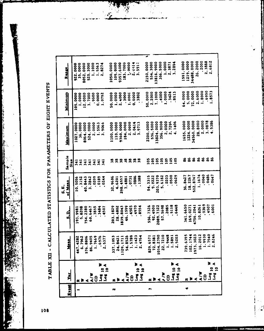
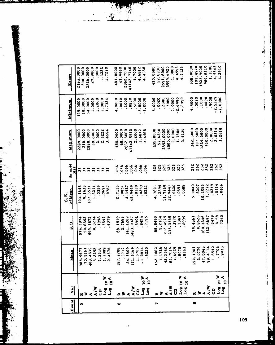
OOOOO_O_ONO_NONO_O_ _
OOOOO_O
_ ON F_
OOOOOO_ O OOOOOO OOOOOOO
oo..o ooooo o-o-o ,
OOOOO_OO_O_O_OOOO_ONO
4 .... M_||
OOOOON_OOOOON_OOOOON_
OOO_O_
OOOOON_ OOOOO _O _O_O_ O_OOO O _O OO_O_ ONOOO_
OOOOO_OOOOOO_OOOOO__O0_ON
M_4_Md_
0000000NNNNNNN
NNNNNNN
NNNNNNN
._ __ • . .
_N_N=N N_N_
_O_OOO _N_OOo O_OOO
d'_g''"
_d_''' __ • • ' _d_ " " '_ NN
__ • . .
_ '4_ " d__ ," " __,'"
_o oo oo oo
I09
,6
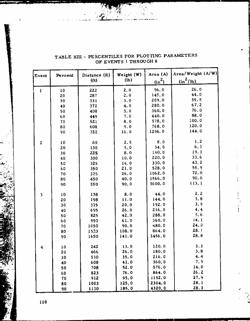
Event
2
4
110
TABLE XIII - PEKCENTILES FOR PLOTTING PARAMETERS
Percent
I0
20
30
40
50
60
7O
80
90
I0
20
30
40
50
6O
7O
8O
90
I0
20
30
40
50
60
70
80
90
I0
20
30
4O
5O
6O
7O
8O
9O
OF EVENTS 1 THROUGH 8
Distance (R)
fit)
222
287
331
372
408
449
521
608
722
6O
130
225
3OO
325
350
375
45O
55O
138
198
375
695
825
990
1050
1523
1650
Weight (W)
(lb)
2.0
2.0
3.0
4.0
5.0
7.0
8.0
9.0
16.0
2.5
5.0
8.0
I0.0
14.0
21.0
26.0
40.0
90.0
8.0
11.0
20.0
26.0
42.0
61.0
90.0
108.0
141.0
242
466
510
608
708
823
912
1003
Ill0 185.ii
13.0
26.0
35.0
41.0
52.0
76.0
95.0125.0
0
i
I
I Area (A)(in21
96.0
145.0
209.0
280.0
360.0
440.0
578.0
768.0
1296.0
8.0
34.0
140.0
220.0
330.0
528.0
1062.0
1566.0
3600.0
44.0
144.0
192.0
216.0
288.0
360.0
480.0
864.0
3456.0
120.0
180.0
216.0
360.0
576.0
864.0
1152.0
2304.0
4320.0
Area/Weight (A/W)
(inZ/Ib)
26.0
44.0
55.5
67.2
76.0
88.0
I00.0
120.0
144.0
1.2
6.1
19.3
33.6
43.2
55.9
72.0
90.0
113.1
2.2
3.8
3.9
4.4
5.6
14.1
24.0
28. !
28.8
3.3
3.8
4.4
7.5
14.0
26.2
27.9
28.128.3
i
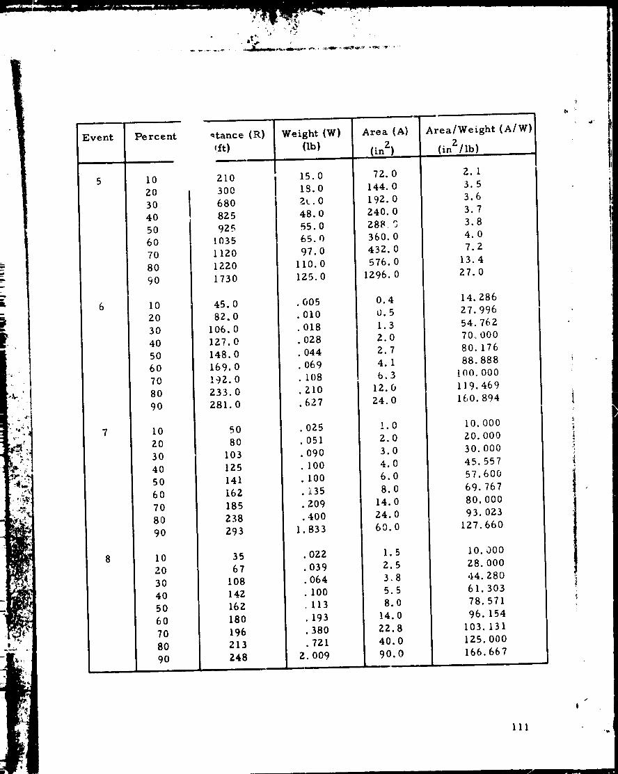
Eve nt
6
7
Percent
10
20
3O
4O
5O
6O
7O
8O
9O
I0
20
30
4O
5O
60
70
80
90
10
20
30
40
50
60
70
80
90
I0
20
30
40
50
60
70
80
90
qtance (R)
_ft)
210
300
680
825
925
1035
1120
1220
1730
45.0
82.0
106.0
127.0
148• 0
169.0
192.0
233.0
281.0
50
80
103
125
141
162
185
238
293
35
67
108
142
162
180
196
213
248
Weight (W)
(ib)
15•0
18.0
ZL.O
48.0
55.0
65.0
97.0
II0.0
125.0
005
010
018
028
044
069
108
ZlO
627
.025
.051
•09O
• lO0
• 100
•135
.209
•400
1,833
,022
039
064
100
113
193
380
721
2.009
Area (A)
72.0
144.0
192.0
240.0
288 3
360• 0
432.0
576.0
IZ96.0
1,5
2,5
3.8
5.5
8,0
14.0
22.8
40,0
90,0
Area/Weight (A/W)
(inZ/lb)
2. I
3.5
3.6
3.7
3.8
4.0
7.2
13.4
27.0
14.286
27.996
54,762
70o000
80.176
88.888
!00.000
119,469
160,894
I0. 000
ZO. 000
30. 000
45. 557
57.600
69. 767
80. 000
93. 023
127. 660
I0.000
28.000
44.280
61•303
78.571
96.154
103.131
125.000
166,667
/
I
III

.,-,tT_ ¸ •. I'll
ooZ
f.,.iIDZ.<
i,==l
Cl
m
P
6 ,,J
.r
30VlN33_3d
Z
0Z
Z00.1
Z0
m
m
Q
[--t
m
8
m
Z
4
0
113
distribution appears to be a better fit. Figures 45, 46 and 47 are examples of
the other plots. From the plots over all 8 events, it appeared that the normal
distributions adequately fitted the distance (EL), and A/W and that log normal
distributions best fitted the weight (W) and area (A). A complete summary of
the fragment data is given in Table XIV, giving the estimated standard devia-
tion (S), and mean (M) for the respective distributions for each parameter in
each event.
A "W" statistic for goodness of fit for each parameter was calculated
using the methods outlined by Hahn and Shapiro (Ref. 36).
The approximate probability of obtaining the calculated test statistic,
given that the chosen distribution is correct, was then determined, and is
shown in Table XV. Figure 48 is a plot of Table XV, and can be used to de-
termine the approximate probability of obtaining a value as low as the calculated
value of "W", given that the selected distribution is the correct one. The
values in Table XVI were calculated usir,g the method and formula outlined by
Hahn and Shapiro (Ref. 36).
Table XVI is a summary of the "W" test on normality for R, W, A, and
A/W for the eight events. The method, and sample calculations for the W
statistic and the probability of obtaining the calcu] ted value of W are given
in Appendices E and F.
Referring to Table XVI, we see that there are 3Z distributions, one
each for R, W, A, and A/W for each of the eight events. The probability of
obtaining the calculated value of "W" is greater than 50 percent for all exceptth_ A/W distributions for events 3, 4, and 5, indicating adequate fits for all
except these three distributions, as it is customary to consider values exceed-
ing Z to 10% as adequate grounds for not rejecting the hypothesis that the data
belong to the chosen distribution. It is interesting to note that each of the
parameters i3 distributed in the same family (i. e., normal or log normal)
across all eight events. That is, distance (R) has a normal distribution func-
tion in each of the eight events, indicating a repeatable pattern.
The estimate for the means and standard deviations for each of the dis-
tributions is given in Table XIV.
D. Methods of Prediction of Range Versus Fragment and
Blast Yield Parameters
1. Determination of Mean Range of Fragments Versus Blast Yield by.
Regression Analysis - The mean distance R ver6us the yield Y in percent and
equivalent pounds of TNT, W_. _ for the 8 events waJ plotted on log-1
paper and is shown in Figures _9 and S0, reopectively. As can be seen,
when events 6, 7 and 8 which are the mixing teats are excluded, there is more
114

e •
e"
mm
<
4:
b4 ._i
0 ._-
D _
, _,_
>,it
o,
Ii,m
_0 ul% N _ e,- 00 0 '_
Z Z Z Z Z Z Z Z
,_0 O0
_P 0"- "% ,m 0",
,.] ,..] _ ,-] ,4 ,J ,J ,J
N "'
,,_ ,g
un N ¢%1 um _1' _1'
N CO _ O" O um
_ O0 ."% '-' (_' "" '='
,,,; ._ =6 ._ -; ¢_ 6 6N "% um un
,..] ,-1 ,_ ,..] ,J ,.,] _ _]
_1' *'_ t'-- N _1' 00 .,0 0"
N _ e,"l II%
p- I',- 0 0 _D ¢,, N N
•I' I',- _ _1' 00 um u% um
Z Z, Z Z Z Z Z Z
_ N N 0 O4 N N0 0 0 _ _ 0 0 0
N N N _ :,t00 e'% 0" ._ I'- _%
tim O 0 N O O -O I"-
4 .-; 4 4 -; ,4 -: :0 "-' 0 _' ,_ 0 0 0
; ® ,,, _ _ = = ,.,,
• .., N i,_ 'e if, ._ I.,- o0
o.3:!
10
>,U
(:
(g
o
.=_,=,,9,oel II
...,I
2
115
,1
• , !̧
Q_
TABLE XV- APPROXIMATE PERCENTAGE POINTS OF
"W" TEST FOR NORMALITY (n = 9)
• _ _ %"
,
-< ..o,°;.
"W" Percentage
•764 I.0
.791 Z. 0
.8Z9 5.0
•859 I0.0
•9Zl 38. Z
•93 5 50.0
•945 64.3
•969 87. I
•978 94.8
•988 99.0
116
$ •
,,. ,°
r r
0
0
°.,4
117
P
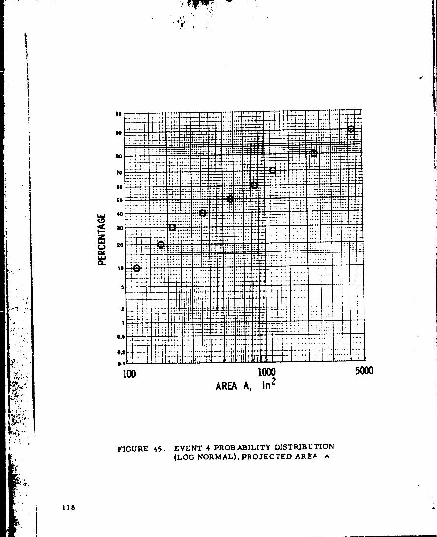
I,
• _ i_, _
q*
4 _
8O
100 1000AREA A, in2
5000
,II
118
FIGURE 45. EVENT 4 PROBABILITY DISTRIBUTION
(LOG NORMAL), PROJECTED ARE_ .'_
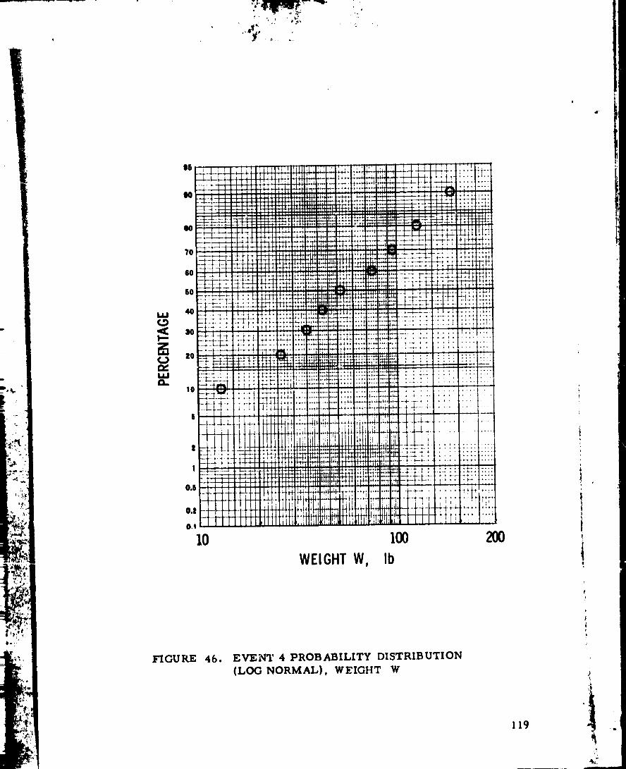
7_+--+ ....
10
HGURE 46.
+J
"I++
_.+.j
.++.+.
+.+.fi*
;[i
iiI.L
Ii
:!+,
4+
.4+1
11
100
WEIGHTW, Ib
EVENT 4 PROBABILITY DISTRIBUTION
(LOG NORMAL), WEIGHT W
119
+ •
("
.II.#L
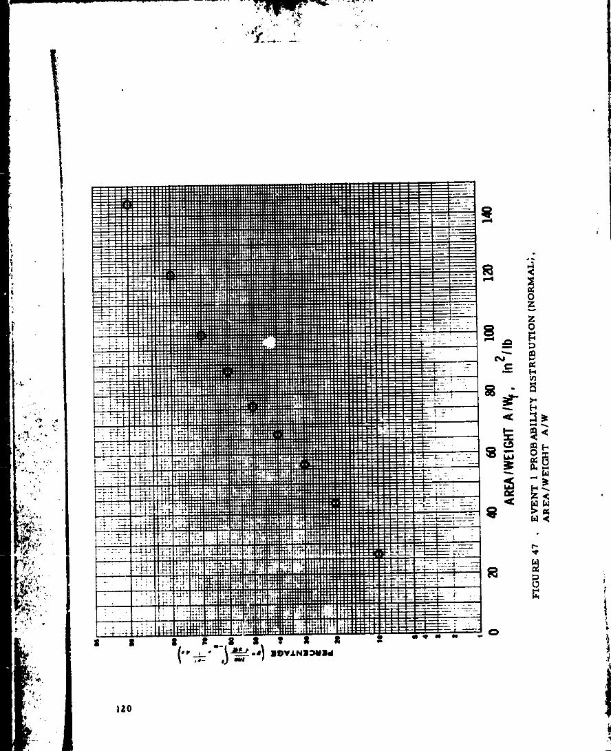
0

• ,r
_dl? ,..
O?
N
7O
10
I0
FIOURE 48.
Illt.I.
il
II11ilIIIII!iw
ii
1"-','4
r:n_'1-4
"4"
_'4
i'
'i
.800 .840 .880 .920"W" STATISTIC
lilll
II111
II
!II
III
zt
Ill
APPROXIMATE PROBABILITY PERCENTAGE POINTS
OF "W" TEST FOR NORMALITY (n • 9)
IZI
?
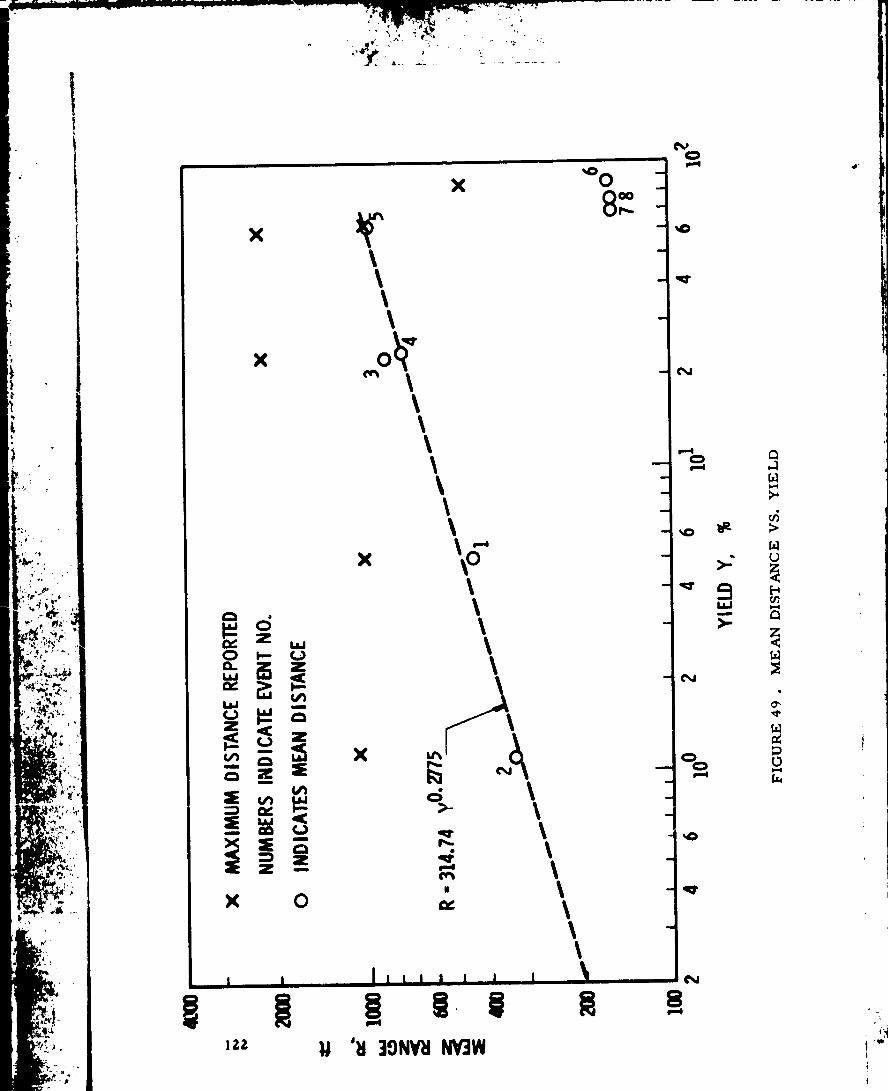
|
x
X
\\
\
X •o 0 -
8_
m
\
+ \z X
l.,J
Z .__ _ z_ _._. x_ z IE
M
\\\\X
IE w <==. _ t.)
X 0
IZZ 'H 30NV'dk_3W
m
° o 0
i
@
d"
0
123
/
i

scatter on the TNT chart than on the percent yield chart. A regression
equation was derive# to describe a linear fit to the points. Events 6, 7 and8 were excluded on the basis that the propellants were mixed differently than
in events I through 5. The equation is:
y0. Z775R = 314.74
This equation should be limited to the range of weights and configurations of
events I through 5.
The line is drawn on Figure 49, and the predicted versus observed
values of the mean distance /or the 5 events can be read from the chart. On
Figure 49, the maximum observed distance is also shown for each event.
In Figure 51,the upper dashed line shows the estimated distance which
should contain at least 95°/0 of the fragments. Table XVII shows the upper 95%
confidence limit (CL} on the estimate of the mean (IV[}, the upper 90% confidence
limit on the estimate of the standard deviation, and the various quantities
necessary to calcldate these confidence limits.
The confidence limit on the mean was calculated using the following
formula:
CL =M +_n tn; 95,i#
n is the number of fragments and tn; 95 is the value of the t distribution with
n degrees of freedom at the 95th percentile.
The confidence interval for the standard deviation was calculated using
the followin|[ formula:
CL =Ex z i - i)Zln ]XZ(n- I);90
1/z(64}
Where Xi is the distance of the ith fragment, n is the number of fragments,
and XZ_n I_'90 is the value of a chi square distribution with n- I degrees offreedor_ _t {_e 90th percentile.
Then, using the new upper confidence level values of }v/ and S, the
range _95 in which 95_o of the fragments should fall was calculated as follows:
A
R95 =M +Stn; 95
The interval frown the mean (M) to _95 is indicated for each event on Figure 51
i
D¸, .<
G •
• mT_
• ,_r T ";C" "
by a bar.
A line was then drawn parallel to the regression line, and just touching
the longest bar. Thus, the distances read from this line could be expected to
encompass at least 95% of the fragments restating from a given yield.
Z. Determination of Mean Ra_ se of Ballistic be
Equations - _ range of afragme_" produced by a missile _xp_osion maydetermined from ballistics eqaations if sufficient information is available
about the initial fragment velocity and fragment characteristics. Specifically,
it is necessary to knov¢ the following parameters:
(1) The fragment mass, M
(z)
(3)
(4)
(5)
The initial fragment velocity, Uf
The initial elevation of fragment trajectory,
The fragment cross-sectional area, A
The drag coefficient for the fragment, C D
(6) The density of air, f) air
Having given these parameters, the range of the fragment may be ob-
tained from the equations of motion solved for the total time of flight of the
fragment. This method is described and the following equations completely
derived by J. J. Oslake, et al, (Ref. 41)for the case of a missile exploding
on the launch pad with the assumption that air density remains constant along
the trajectory of the fragments produced. Only drag and gravitational forces
are assumed to act ¢ the fragments where
2 (65)
F d = - (11z) 0 U A C Fg = - M gz D'
are the vertical _on_poncnt of the drag force and the gravitational forces,
respective])'. ( 0 = Oai r and U = vertical velocity oi the fragment. } TheZ " a
equation of motion for vertical acceleratxon m ybe integrated to obtain t
as a function of U , which givesZ
1 - 1tr = _ tan (Uzo
for the case in which U = 0 (i.e., t.. is the time of rise for the fragment).z.. vertica_ fra_cqnent velocity and
In Eq. (66) U is the inttxalZO
(66)
(½}°airACOc = M
The equation of motion for the fall of the fragment may be similarly integrated
to obtain1/z
_ l _ zCZM ZCZM - 1] ] (68)tf z.g._. _n Ze - 1)+ [(Ze - l)2
whe re
1[ 1 ]ZM= -- _n c_c cos ( t )r
(69)
The total time of flight of the fragment is
T = t +tfr
(70)
where t and tf are functions of initial conditions only. Finally, the equationsof motio r for raclial acceleration of the fragment may be integrated to obtain
the range R in terms of _ :
l m ) (7 1)R = -- Ln (l + c URoc
The range may be determined from our initial parameters, since c is a
function of M, A, C , Pair (Eq. (67)); URo is the radial component of the
given initial velocity, Uf:
VRo = Uf cos (72)
VZo = Uf sin
and thus is a function of Uf and O; and _ is a function of initial conditions Uf,
0, c and g.
A computer program in FORTRAN IV which computes fragment range
as a function of the independent parameters mentioned above is given in
Appendix H. This program was checked against the re suits of J. J. Oslake,
et al (Ref. 41); the check appears in Appendix H. The symbols used in the
program as well as the input and output parameters are also discussed the re.
This method of range prediction requires considerable information
about the fragments emanating from the missile explosion. In general, the
IZ8
,_ i_
initial fragment velocity, U , may be determined by one of the methods describ-f
ed in Section III.B. Fragment mass, cross-sectional area, and drag coefficients
must be determined empirically. Drag coefficients for fragments at various
velocities are described by L. D. Heppner and J. E. Steedman (ref. 4Z).
Coef_'icients for regular shaped projectiles (spheres and cylinders) are de-
scrxbedby E. Richards (ref. 43). A correlation between range predicted by
this method and that determined statistically for a "mean" (or average) frag-
ment from the PYRe test data, event 062, is given in Section IV.E.
E. Correlation
I. Standard Statistical Tests
a. Standard Deviation Versus Mean Distance - Figure 5Z is a
plot of the standard deviation of the distance versus the mean distance R for
each of the eight events. As one might expect, the standard deviation in-
creases as mean distance increases.
b. Results of Scaling A/W Parameter - From Appendix B,
formula Bl3 is:
, Af/Wf2/3 (73)G7 -
where A. is tbe fragment cross-sectional area -'(in2),!
ment weight.
and Wf(lb) is the frag-
F_gure 53 is a plot of the geometric means of A/W versus geometric
mean distance_l_3(ft) for the eight events. Figure 54 is a plot of the geometricmeans of A/W _/ versus geometric mean distance.
The points,
regression analysis which resulted in the prediction equation:
= 9.864(A/W 2/3) 0.78
^ (in2where R is the mean range (ft), A is the area of the fragment ),
is the weight of the fragment (Ib).
excluding events 3, 4 and 5 have been fitted to a line with a
(74)
and W
The exclusion of events 3, 4 and 5 can be justified on the basis that
A/W for these three events were noticeably low in probabilit_ of belonging to
the log normal family of distributions, while A/W for the other events showed
a high probability of belonging to the log normal family.
Comparing the points in Figure 5Z with those in Figure 54, it is ob-
vious that, in this case, scaling of the A/W parameter improved the correlation
0
130
¢
0
0
I I I I
$ NOI.I.VIA3GO_IVONVI$
8
E%
.,,..
b2•
v
3...,.,,..
0 7
Z
- o z5:
t I I n 3 45
2_-
10 --- 2 4
DISTANCE(GEOMETRICMEAN)_, ft
FIGURE 53. GEO_T RIC MEAN
AN DISTANCE
A VS. GEOMETRICW
131
'k
_t
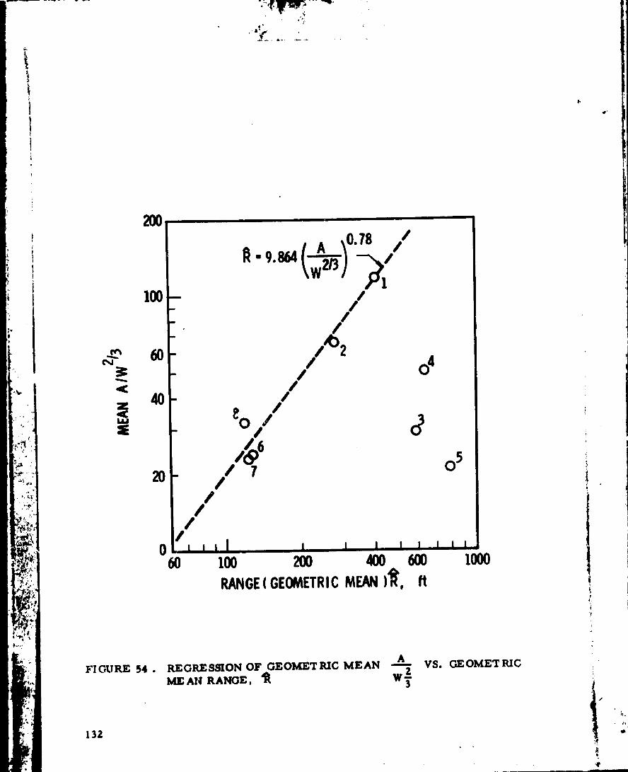
200
I00
_" 60
FIGURE 54.
13Z
2O
• A ,0.78 //
m
.m
m
: /" I
_ /7/
/0 I
' If|00 i , i i i200 _0 60ORANGE( GEOMETRICMEAN)_, ft
REGRESSION OF GEOMETRIC MEAN W"_ VS.MEA_ RANGE,
o 5
i I
I000
GE OMET RIC
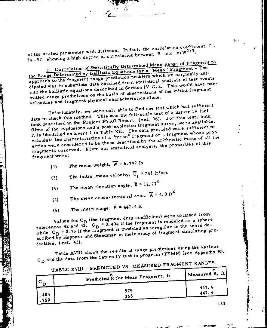
i
of the scaled parameter with distance. In fact, the correlation coefficient, _ ,
is •97, showing a high degree of correlation between R and A� WZ/3"
isticall e oforrelation of Star __-:_' Frajzment - The
Z. C or.__ " ns for a Mean __
Determined by..Balllstlc E_approach to the fragment range prediction prc)blem which we originally anti-
cipated was to substitute data obtained from statistical _nalysis of test events
into the ballistic equations described in Section IV. C.Z. This wou].d have per-
mitted range predictions on the basis of observations of the initial fragment
velocities and fragment physical characteristics alone.
Unfortunately, we were only able to find one test which had sufficient
data to check this method. This was the full-scale test of a Saturn IV fuel
tank described in the Project PYRO Report, (ref. 16). For this test, both
films of the explosions and a post-explosion fragment survey were available.
It is identified as Event I in Table XII. The data provided were sufficient to
calculate the characteristics of a _*mean" fragment or a fragment whose prop-
erties we.'e considered to be those described by the arithmetic mean of all the
fragments observed. From our statistical analysis, the properties of this
fragment were:
(I) The mean weight, W" = 6. 797 Ib
(2) The initial mean velocity, _f = 741 ft/sec
(3) The mean elevation angle, 0 = 1Z. 77 °
(4) The mean cross-sectional area, _ = 4.0 ft z
(5) The mean range, _ = 447.4 ft
Values for C D (the fragment drag coefficient) were obtained from
references 4Z and 43. ?D = 0.404 if the fragment is modeled as a sphere
while C D = 0.75 if the :ragrnent is modeled as irregular in the sense de-scribed ,by Heppner and Steedman in their study of fragment simulating pro-
jectiles, (ref. 42).
Table XVIII shows the results cd range predictions using the various
C D and the data from the Saturn IV test in progr.m (TEMP) (see Appendix H).
TABLE XVIII pREDICTED VS. MEASURED FRAGMENT RANGES
^ Measured R, ft
404
_750
Predicted R for Mean Fragment, ft
579
353
447.4
447.4
133
.t
It can be seen from these results that reasonably accurate range values may be
obtained if an appropriate C D is chosen.
This range prediction method could be more useful if the fragments
were broken down into classes of narrow mass ranges whose mean velocity,
elevation angle, etc., were obtained from empirical considerations. Then
a predicted range mapping could be made, as a function of yield, with the use
of these ballistic equations. To do a complete empirical study, however,
would probably require arena tests using models of the actual missile tanks.
,.t
. ¢
134
\
V. EFFECTS OF FRAGMENTS
A. Introduction
It is desirable to have the capability to predict the probable damage
levels to humans, structures, vehicles, etc. at various ranges from an ex-
ploding missile. Damage can be produced due to the blast wave emanating
from the rupture of the missile or the interaction of the blast wave with ob-
jects surrounding the missile.
Damage caused by blast waves has been extensively studied and is a
result of the peak overpressure or impulse o_ the blast wave depending on the
nature of the "target". Ref. 34 gives examples of this kind of data for damage
to humans as a function of peak overpressure. Since peak overpressure is a
function of range and yield, dan_age levels can be associated with these para-
mete r s.
In order to predict damage as a result of fragmentation, it is necessary
to know the value of the terminal ballistic parameters of the fragments (i. e.,
velocity, range, mass, cross-sectional area, etc.). Insofar as the value of
these paran_eters can be determined from the characteristics of the missile
explosion, damage levels can be predicted as a function of yield.
In Sections II and IV of this report, we have tried to investigate
methods of determining fragment initial velocity and range by statistical and
deterministic methods. By and large, however, the empirical data are not
sufficient to cover the fragment damage problem on the basis of existing mis-
sile explosion data. A great deal of work has been done, however, on the
problem of fragment damage from bomb explosions. We feel that much of this
work is applicable to the exploding missile problem, even though the initial
fragment velocities for the exploding missile would be prirnarily subsonic,
whereas those for exploding bombs are usually s apersonic.
A considerable amount of investigation has been made of what the ter-
minal ballistics characteristics of a fragment must be in order to cause
damage to various "targets". Equations for penetration of wood, steel, etc. ,
of various thicknesses (as well as human simulators) have been developed
from empirical data which may be used to predict damage levels as a function
of fragment mass, velocity, and area. The probability of damage to these
targets at any range would be a function of the probability of arrival of a frag-
ment meeting the minimum specifications for the damage equations. The
probable fragment damage for a given range as a result of a missile explosion
is thus predictable when these two parts of the problem are solved:
(l) The probability of arrival at any given range of a fragment
of specified mass and cross-sectional area, velocity, etc.
135
,<
!_t
.4
(z) The probability of penetration or damage to a specific
"target" struck by a fragment of the specified mass,
cross-sectional area, velocity, etc.
B. The Probability of Arrival of a Fragment of Specified Characteristics
Versus Range
I. Fragment Characteristics - It is necessary to characterize the
fragments in various ways such that trajectory analysis will allow a ma_ 9ing
of fragments from a unit solid angle about the explosion to a unit ar_a on the
ground surface at some range, R, from the explosion center. Specifically,
it is necessary to know the fragment mass distribution; cross-sec_*onal area
or projected area distribution, and the drag coefficient for the fragments.
Many of these characterizations are obtained from empirically derived
equations for bomb studies. One accepted equation in bomb studies relating
fragment mass and area is:
M = k A31z (TS)
where M is a fragment mass, A is its cross-sectional area and k is some
constant ( ref. 44). For a mild steel fragment of "flattened" shape k = I. 45,
for instance(where A is taken as the mean projected area of the fragment)
(ref. 45). The distribution of fragment masses may be given by:
N(M) =Noexpl. (M/I/)Y } (76)
and I/_i..':: _., where N is the number of fragments with masses greater than M,
"_'_$i_:'_ equals I, 1/2, or I/6 the average fragment mass depending on whether Y
:-'::_ equals I, 1/2 or 1/3, respectively (ref. 46). Equation (76) actually thus
mj[_1_ _ , defines three different mass distribution laws which are applicable for various
!'"_l_ _. types of explosions (for a thick walled shell in a three-dime!sional breakup,
• * i::_: U equals the average fragment mass and Y = I, for instanc ).
Appropriate values for the drag coefficient must be ,hosen in order to. calculate the aerodynamic coefficient in the drag force equation, c, [see
'_'" " Section III. B-I, Equation (67 0 • Some values for C D were given in Section
i':'l_ IV-C. For bomb tests, the values C D :.48, . 60 for sub- and supersonic fra_-
- ".]_i__ meat velocities seem to be common (Refs. 46 - 48) giving:
li_;_ ">" Fd ='0031m'I/3 U 2 subsonic (77)
,-. I13 U zF d = . 0030 m" supersonic
for the drag forces (mass in engineering units and velocity in ft/sec. )
136

Empirical equations such as those obtained from bomb studies should
be developed for missile explosions where the fragments are larger and have
lower initial velocities. Until such equations are developed, some good pre-
dictions can probably be made using the equations relating to subsonic velocities
for bomb fragments of relatively large mass.
Z. Trajectory Analysis - A trajectory analysis may be carried out on
fragments of known characteristics as was demonstrated in Section IV-C.These techniques result in a range calculation but not a terminal velocity cal-
culation. Solution of the equations of motion for a fragment traveling at the
speed U along its trajectory:
X + 8 VX +g sin_ =0 (78)
y + _VY +gcos a =0
where B is the aerodynamic coefficient with the same definition as c in
Equation(65). Sections II-B, X and _ are local coordinates of the fragmentat time t measured in a coordinate system moving with the fragment,__ and a
is the elevation angle of the fragment relative to the _rajectory in the X, Y
coordinate system) will yield the terminal velocity and range. These equations
are solved by Feinstein and Nazooka (ref. 48) using a technique in which
gravitational effects are a perturbation on the drag equations.
•. • Z (79)X +8 X =0
O
For trajectories in which the fragments had an initial elevation angJe less than
that required for maximum range (low register trajectory)
X = ('Xo + "Xp) cos _ o " _ sin (_o (80)
whe r e
o
_p = - (g/Z) t z sin (I (I + u13)l (I + u)
u=SV t0
"_ = (g/Z) t z cos (l[u (I + u/Z) - log (I + u)]
t is the time of flight obtained from the equation
-- +_ sin • ÷Y" COl _ "0Y "Xo p o o
/u z
(81)
(SZ)
i
i
t
137
q
and _ = ot is the initial elevation angle. Solutions for other trajectories areO
obtained numerically for time interval steps t in which displacements occur.
m
X cos ot- Y sin a
X sinot+ Y cos ot
(83)
Terminal velocity can be obtained by straightforward differs ntiation of Equa-
tions (78) and _79} with respect to time, t, but Feinstein omitted this step.
3. Mapping From Explosion Center to the Ground Plane - Feinstein
uses Eqs.(80) through (83) to map the number density of fragments from bombs,
n., in a mass internal i Irom those passing through an area element Ro2COS _o
AZg A ot on a hemisphere immediately surrounding the bomb, to those land-O O
ing in an area on the ground plane at range R, R h gh R. For ni density
of fragments at the elernental area at the hemisphere and n. density of frag-zmeuts at the elemental area at the ground plane
ZR cos ot
o o o (84)
n. " n. 1 Iz 1 R dR/d oto
The trajectory equations and initial conditions on the fragments yield the value
for R + dR/d0t . n.°, R o, and ot are related by fragment arena data.O I O
In a simpler view, n.° could be obtained from Eq. (77) and the explo-
sion could be assumed to havle spherical symmetry. As in Feinstein's calcu-
lation, Eq. (75) would be assumed to hold. Values for C D would be chosen
appropriate to the type of fragments expected from missile explosions and the
number of fragments in a mass interval classification as a function of range
would be calculated using Equation (84) and trajectory equations. Finally, the
probability of impact on a target of area A i of a fragment in mass internal i
may be obtained from Poisson statistical equations, and the probability of
damage for a given "target" would be assessed on the basis of vulnerability
criteria and the flux of fragments as a function of range meeting those criteria.
Feinstein has actually solved the problem of hazards to humans _s a
result of several types of bomb explosior, s using his technique. His results
(for the assumption that fragments of 58 ft-lb or greater of energy are hazard-
ous to humans) are given in the form of probability of injury contours. We
suggest that this technique or a simplified version of it coupled with more com-
_.., plete data on missile explosions could be used to produce similar results for
the missile explosion problem.
I !• 138

C. Vulnerability Criteria
1. Structures - When a fragment emanating from an explosion arrivesat the "target", the degree of damage it will produce is generally a function of
its terminal velocity, mass, cross-sectional area, and the characteristics of
the target. The relationships between these quantities and sorve measure of
damage level for structures are empirical equations which are unrelated to the
source of the fragn_ent. Thus equations of this type which have been exten-
sively developed fo," prediction of damage from bomb fragments would be
applicable to the exploding missile problem.
An accepted form for vu!nerabil'.tY equations is:
8e A (SS)
U =k yM
where U is the fragment velocity. A is the presentation area of the frag-
ment, M is the fragment mass, and e is the thickness of the target mater-
ial. This equation of the "de Marre type '| predicts the terminal velocity of a
fragment required to penetrate the distance e into a structure where the con-stants a , 8 , Y , and k are a function of the material from which the struc-
ture and _ragment are made. These constants are obtained empirica11y for
various materials, and example values for the constants can be seen in
Table XIX.
Some fragments from missile explosions are sufficiently large that
penetration of a structure is not likely to be the primary damage mode. For
svrh fragments the kinetic energy of the fragment may be of most interest
in relating to probable structural damage. In some cases, the mass of the
fragment would be suffi,:icntto crush a structure were it to land on top of it.
Clearly the damage potential of fragments from missile explosions is related
to the types of structures which are in danger of damage and the materials
and techniques used in their construction. To classify and investigate all
such structures is beyond the scope of this report.
2. Personnel - The simplest criterion for fragment damage to per-
sonnel is the so-called '_inetic energy criterion" which is attribed to Cranz t
"Lehrbuch der Ballistik". This criterion states that a fragment having 58 ft-lb
of kinetic energy is capable of producing a human casualty. This criterion
was widely used during World War II to predict casualty levels and was used
by Feinstein ( ref. 44) in 1972 to obtain probabLlit_/ of casualty contours from
the equations described in Section V-B. Like most empirical values its
justification is that it seems to give correct results more often than not.
,39 1I
t"
140
_0
0
.1
0
L)I
XI.'4
X
N0
_0 r_
w
w _
opl
om,4 .,.¢ ,m-¢
J
0 ¢,
Other empirical values for the characteristics of fragments which
will produce an incapacitating wound have been obtained from
M I U I = M 2 U_(86)
where M is the mass of one of two fragments, i, and U. is its velocity.
This equation attests that having determined the mass an_d velocity of one
fragment capable of incapacitating personnel all other fragments satisfying
Eq. (86) also would be potentially incapacitating. The value for ct is various-
ly given as Z. 5, 3.0, etc.
A "standard" assessment for fragments capable of producing casualties
which has been widely used, is the wood penetration test. In this test, pine
wood panels of thicknesses ranging from 1/2 to 1 inch are present in the range
of fragments from an explosion. Where the panels are perforated, it is
assumed a casualty would i:ave occurred, otherwise not.
At this time, itwould seem that acceptance of an empirical "standard"
such as the kinetic energy criterion of 58 ft-lb would be th, best idea in inves-
tigating potential fragment damage to personnel as a resul: of a missile explo-
sion. Acceptance of this value would allow the use of bomb fragment data
which was based on that value. Ultimately, itwould seem reasonable to try
and obtain data on the probability of injury as a function of kinetic energy
of the fragments, and extend existing bomb fragment data to the case of more
massive fragments of the type which may be encountered in missile explosions.
141
• _',_I 5111'
I °
t"
i
Vl. DISCUSSION OF RESULTS
A _Jajor part of the work consisted of efforts to retrieve data relevant
to the basic problem of fragmentation of liquid propellant vessels by literature
search and visits to various government and private agencies. We believe
that we were successful in assembling the majority of such data which are still
available in the literature and in the files and archives of NASA and Department
of Defense agencies, and in entering the data in the ASRDI data bank. The
primary sources of data were the Project PYRO experiments (refs. 15- 17),
recent experiments conducted at NASA-Kennedy Space Center (ref. 39), andseveral accident reports (refs. 24 and 38). These sources, however, yielded
only partial information with one exception. They gave eithe_ r d_ta on initial
fragment velocities together with measured blast yield, or data on final loca-tions, masses, and shapes of fragments. The only exception was PYRO Test
#62, which gave both types of data.
The following observations are appropriate in order to place the results
obtained from fragment velocities measured from I=_RO films into the proper
perspective.
(1) Velocities were measured for many different combinations oftank size (and total propellant weight), tank height to diameter
ratio, propellant types and test _-pe, that is, confined by
missile or confined by ground surface.
(z) Velocities were measured at different positions in space de-
pending on where they were first sighted. The instantaneous
velocity of the fragment immediately atger sighting was deter-
mined, and an average velocity of the fragment was determined
by assuming that it traveled in a straight line from the centerof the tank to a point at which the fragment was first sighted.
No attempt was made to estimate the initial velocity of the frag-ment at the tank wall from the velocities calculated at a later
time.
(3) Velocities determined from data obtained from a single camera
view are only approximate because the fragments often had
components of velocities directed toward or away from the
cameras which could not be detected. The necessary assump-
tion that such fragments travelled normal to the camera lens
axis introduced possible errors of +0% to -30%, i.e., velocitie._
were generally underestimated. Likewise the coordinates of
the fragment in terms of the radial position, height, and azimuth
angle could not be determined accurately.
14Z

(4) For fragments which could be observed from two differentcamera locations (spaced 1Z0 ° apart), their true trajectory
and thus their true velocity could be obtained. Unfortunately,
fragments were difficult to identify in more than one cameraview and so true velocities were obtained for only a few frag-
me nts.
(5) It was rot possible to relate on a one-to-one basis fragment
velocity and heading with fragment size, shape or final range.
In spite of these ]imitations to the fragment velocity data, we feel that
the data we obtained were very useful, and reasonable corrclations with pre-
dicted values of velocity have been obtained. Nevertheless, we feel that the
velocity data warrant additional study directed perhaps toward predicting the
initial fragment velocities and those we had measured. We also feel that con-
trolled experiments _hould be performed which would permit correlation be-
tween measured fragment velocities and the resulting missile masses.
Techniques could be employed to allow initial velocities to be correlated with
the final fragment size, weight, and position. An overhead camera locatedabove the event with a wide field of view should facilitate velocity measure-
n_ents and tracking during such a test. Tag markings would a/so facilitate
fr_ g_r-nt identification.
The fragment initial velocities, as estimated by the calculated para-
hinter Uf (see Section III) for the four pooled groups (CBM-LOz/LH 2, CBM-
LO_/RP-I, CBGS-LOz/LH z, CBGS-LO?,/RP-I) were fitted by log normaldistributions. The means and standard _eviations of these distributions are
given in Table VIII.
The goodness of fit test, using the "W" statistic (ref. 36) showed pro-
babilities from .415 to .99 of obtaining the calculated values of W, giving
us no cause to reject assumed distributions. Thus, the log normal distribu-
tions appear to be an adequate fit for the fragment initial velocity distributions.
These probability density functions can be used to represent fragment
initial velocity densities for the subject propellant combinations within the two
configurations, CBM andCBCS.
Complete det3ils of all data sources and analyses are given in the main
bod'! of the report.
In Section If, we reviewed data pertinent to blast yield for propellant
explosions, and also presented methods for estimation of blast yield and thefree-field blast wave properties for various types of explosions and propellants.
These me_hods relied heavily on the extensive series of test results from
Project PYRO (refs. 15-17), but also incorporated much of the physical
4
143b
t
s
insight apparent in the work of Farber and co-workers (refs. Z7-30). Themethods allow estimation of blast wave peak overpressure and impulse,
given propellant type, total propellant weight, type of accident, mixing time,and distan:e from the center of the explosion. Predictions are limited, how-
ever, to the range of scaled distances of the PYRO tests. A major difference
in our prediction methods and those of reference 17 is in zhoice and scaling of
ignition time. We believe that the scaling for this time assumed in references
15 and 17 is not verified by the test results, and discuss this point at some
length in Appendix A, together with a dimensional analysis of ignition time
scaling.
Density functions for fragment distance R, weight W, area A, and
area/weight A/W, were estimated for each of eight events. A complete
listing of the form and estimated parameters is given in Table XIV. Goodness
of fit tests using the 'W" statistic supported the selected density functions,in all but 3 cases out of the 3Z. These three cases were A/W distributions for
events 3, 4, and 5.
The form of the density functions was constant for each parameter.
That is, for all eight events, R and A/W followed normal density functions,
and W and A followed log normal distributions.
Distance R versus percent yield Y for events 1 through 5 shows a very
good correlation in Figure 48. A prediction equation was derived, and is:
^ y0. Z775R = 314.74 (63)
Confidence intervals were calculated for the means and variances for R for
each of the eight events, and are shown in Table XVIII. In addition the 95th
percentile was calculated for R for each of the first five events, and is shown
on Figure 51.
Using Equation C13 from Appendix C, dimensional analysis for fragment!
trajectories, a new parameter G 7 was calculated:
, Aflwf zla (73)G 7 =
Plotting the geometric mean distanc_ P of events 1, Z, 6, 7 and 8 ver-
sus Gi (Figure 54 demonstrated a good correlation between these two variables),
the scaling of W by taking the 2/3 root brought the distance R into a good' A second prediction equation,linear correlation (on log-log paper) with G 7 .
^ A/W213)0.78R = 9. 864 ( (74)
results in a correlation of 0.97. Thus, within the limits of th, accuracy
144
J
.0
!

• ,_ _-w +,
r __ _ I• +
+_P,+. + +ii,+ _ + ' " * +
+,
allowed by the fragment data available from these^ 5 events, the predictiov
equation could be used to predict mean distance 11 for a fragment of given
maximum projected area A, and weight W.
Data sources and analysis are given in the body of the report. The
damage potential from fragments as a function of range, for exploding missiles,
can be as important a consideration as the damage potential due to the blast
wave. To obtain useful data such as probability of damage as a function of
range for various missile types and "targets 'I of interest, some criterion for
damage to the particular target must be accepted and the probability of arrival
at any given range of a fragment meeting that criterion must be calculated.
The former can perhaps be accepted from bomb fragment damage studies,
although fragments from liquid propeUant explosions are larger and slower.
The latter must be obtained frorn empirical equations developed to define the
distribution of fragment characteristics at the instant the missile explosion
occurs and from suitable solutions of the trajectory equations. Using these
techniques, a °Wmapping" of the fragments from missile to target and probab-
ilia/ of damage to a specific target as a function of range may be calculated.
We suggest an expanded data base relating to distribution of fragment charac-
teristics from missile explosions. The supplementation of bomb fragment
data to cover larger and more massive fragrn _,nts will probably be necessary
before accurate damage probability maps can be made.
+4
+
}
145 ,$
1,
VII. C ONCLUSIONS
This report presents the results of an extensive study of fragmentation
effects of liquid propellant rockets or vessels which explode after accidental
mixing of the propellants. The work was entirely investigative and analytic,
and included no experiments.
Some specific conclusions are as follows:
(I} Accident reports and results of tests simulating accidental
explosions provided a significant source of data on fragmenta-
tion effects of exploding liquid propellant vessels.
(z) Data on initial fragment velocities, masses and shapes of
fragments, and ranges of fragments showed wide statisticalvariations. When the data were fitted to statistical distribution
functions, however, good statistical fits were obtained for these
parameters or combinations of these parameters. In some
instances, the combinations of parameters were chosen by
dimensional analysis.
{3) Methods were developed or adopted for prediction of blast
wave properties, initial velocities of fragments, and fragment
range. These methods were compared with data and appeared
to give reasonably good correlation.
(4) Some approximate methods for estimating damage to various
"targets" by impacting fragments are presented. These could
not, however, be correlated with data obtained during the data
retrieval part of our work because no data were available
on :erminal (or impact) velocities of fragments from bursting
propellant vessels.
{5) The analyses and empirical fits to data inc_'uded in this report
do allow prediction of blast yield and subsequent fragmentation
patterns and velocities for the common propellant combinations
over a wide spectrum of type of accident, weight of propellant,
and time of ignition.
We believe that the work reported here constitutes the first relatively
comprehensive study of fragmentation effects from exploding liquid propellant
vessels. As noted above, predictions can be made of so,he of these effects
using results from this report. But, there are limitations imposed by limita-
tions in the fragmentation data - which has, after all, been retrieved from
sources in which study of fragmentation effects was secondary or even entire-
ly incidental. There seems to be little doubt that one could better test the
146
w
prediction methods presented here if he were able to design and conduct exper-iments with the specific l_rpose of observing and measuring fragmentation
effects. .
147
t
L
./ ..
/
0 . ,t
VIII. REC OMME NDATIONS
The results of this study can, we believe, form the basis for develop-
ment of relatively simple methods of assessing hazards to people and damage
to facilities from the impact of fragment from liquid propellant explosions.
But, the study does not in itself generate such methods because its primary
aim was the collection and analysis of frag_nentation data from past tests and
accidents. We have pointed out previously that non_..__eof the data collected
came from experiments designed to obtain initial or terminal fragment effects.
There is also an almost complete lack of terminal ballistics effects data or
methods _or assessing hazards of the relatively large, odd-shaped, low-vel-
ocity fragments which predominate in liquid propellant explosions. The
authors therefore feel that, although simplified methods for overall estimation
of fragment hazards can be generated, some additional experimental work
would be very desirable to validate these methods.
We recommend the following studies:
(1) sing the initial velocity prediction methods developed here,
the statistical fits to data on fragment mass and shape, and
exercising the trajectory equations of Section IV, expected
variations in impact velocities for a spectrum of fragrne nts
could be computed for a number of hypothetical explosions.
These "Lrnpact conditions could then be overlaid on expected
densities of human observers or bystanders and on nearby
structures to estimate fragment hits. Using the very much
oversirr, plified assumption that a fragment hit on ,_ person
is a kill, or that a fragment hit on a structure causes some
specified dollar damage, each "scenario" could then be
assessed for fragment kills and property damage. In this
way, a simplified damage assessment model could be gen-
erated, based on the work in this report. It is recommended
that this be done, but that the user be strongly cautioned that
the model could be considerably refined and improved, if
better data were available in certain areas.
(z) A careful set of small-scale experiments be designed to obtain
more accurate initial velocity data for tests simulating several
types of accidents. Vessels or nearby objects should be
carefully designed to produce fragments of known geometry
and size, and their motions followed with at least two high-
speed cameras. Such data shoudd serve to improve the data
presented in this report, with much more "two-view" data
yielding accurate trajectories.
,. 148
(3) As a part of the initial velocity experiment_, accurate
missile maps should be made to determine fragment impact
locations. The pre-formed fragments should be carefully
marked so that impact !ocations of many of the fragments
could be correlated with initial velocities and launch angles.
(4) Studies of the terminal ballistics effects of impacts of relative-
ly large, slow fragments of irregular shape would be very
desirable for animals (to make estimates for humans), and
for a variety of structures. Cost might be prohibitive. Some
analytic studies could well provide partial answers, however.
The order in which the above recommendations are listed is also our
suggested order of priority. The first study is purely analytical, but yields
an appro._imate hazards assessment method. The other three are primarily
experimental, and serw_ to generate data which should refine the method.
149
0
i!
i APPENDIX A
MODEL ANALYSIS FOR MIXING OF LIQUID ROCKET PROPELLANTS
I
In the Project PYRO studies, a basic assumption was that, for any par-
ticular type of simulated accident, the time of ignition to produce maximum
blast yield could be scaled as
I13 (A1)"t = t/W
where T is scaled time, t is time of ignition delay after missile failure, and
W is total weight of propellant in the missile. It is not clear that this is the
proper scaling, and no model analysis is presented in the PYRO final reports
to justify such scaling. There are instead statements that the experimental
data appear to agree with this scaling, but the inherent scatter in blast yields
makes this conclusion doubtful. We thought that a model analysis should be
conducted to ascertain, if possible, how ignition times for maximum yield
should scale.
From both the Project PYRO work and Dr. Farber's work, it seems
clear that intimate mixing of fuel and oxidizer is needed to maximize the blast
yield for a given type of accident. The time for ignition must be great enough
to allow as much mixing as possible, but not so great that all of the most
volatile liquid can have evaporated. The physics of the processes which occur
on mixing of LH 2 and LO Z, RP- I and LO Z, and LH_/RP- I/LO Z have beenstudied most exhaustively by Farber andhis associates. They have, however,
considered the dynamics of impact or other accident leading to the mixing in
only a cursory manner. To conduct a model analysis, we should be able to
list the physical parameters affecting this problem, and their dimensions,
which is the prerequisite to conduct of the analysis.
A number of the physical processes which occur are a function of the
particular propellant combinations, and conditions just prior to an accident,rather than the det._ils of the accident. These processes should be governed
by parameters which will be common to all possible types of accidents, and willthus be considered fi-_t. Those propellants and oxidizers which are cryogenic
will be essentially at their boiling temperatures, while fuel such as RP-I will
be at or near the temperature of the ambient air. Once the propellants start
to mix, violent boiling of the colder liquids will occur, while the warmer
ones will be chilled and perhaps frozen. The processes will involve conductive
heat transfer, convective heat transfer, and eventually radiative transfer to
the ambient atmosphere. Gravity is perhaps important in convective processes
and in rlte of upward migration of bubbles formed during boiiing. Latent heats
of fusion and boiling are obviously important, as are temperature differences
150
t
i
, r_ ;
and gradients. Parameters affecting these processes, and their dimensions in
a M, L, T, g (mass, length, time, temperature)system are listed in Table 1.
To complete the list of parameters for model analyses, we must con-
sider specific types of accidents, and also add other parameters known to
affect the blast yield. Consider first the case identified by PYRO as CBM
(confinement-by-the-missile). This case is shown schematically in Figure A1.
iVul
L Do
COMMON
BULKHEAD
Vu2
M2
FIGU RE A 1.
SCHEMATIC OF CBM CASE
A rupture is assumed to occur in the common bulkhead, idealized as a
circular opening of diameter D O• Oxidizer then spills through this opening
under the effects of gravity, and mixes with the fuel. Geometry of the tankage,
ruptured area, distance for oxidizer to fall, static head to force oxidizer
151
i
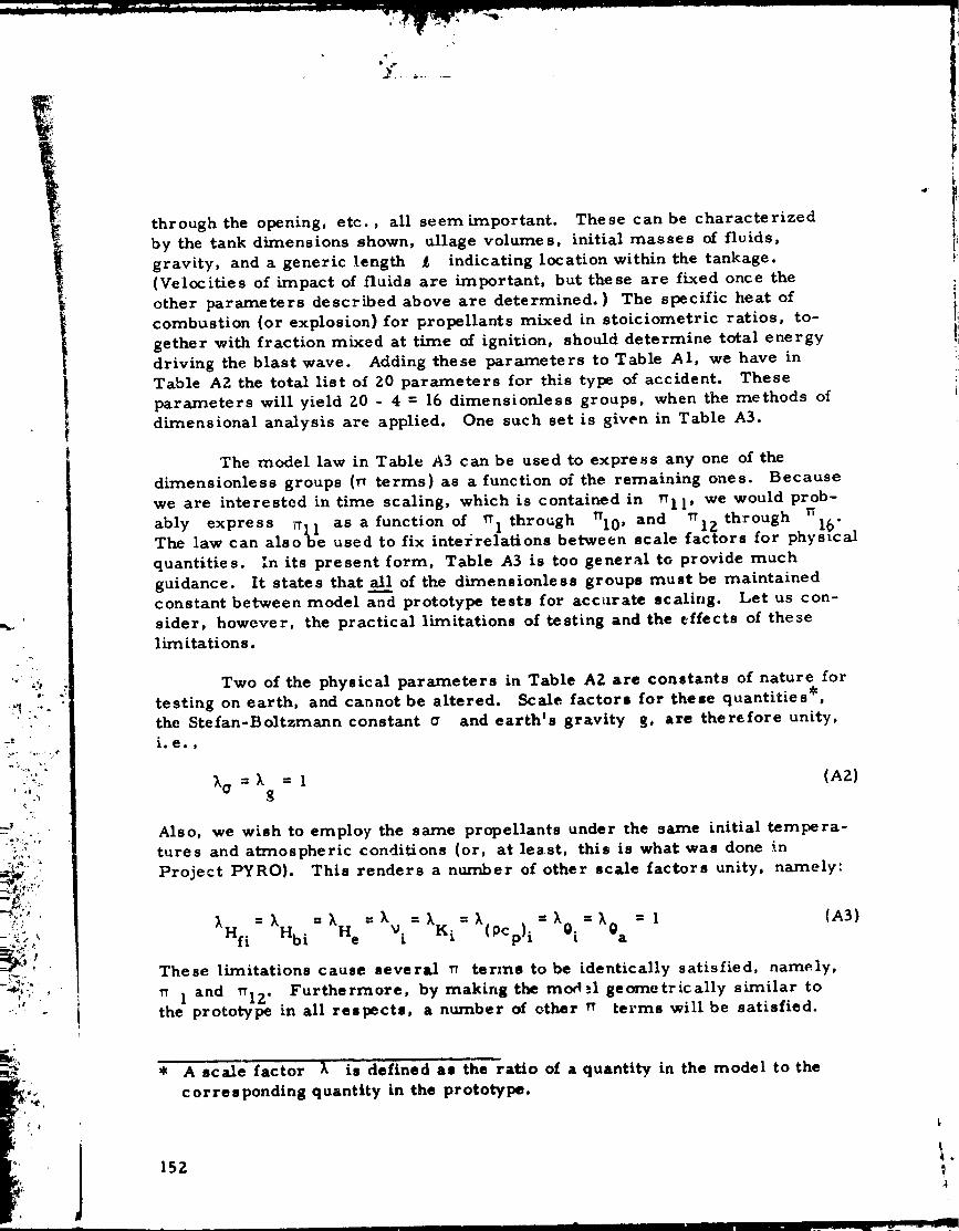
J
i
through the opening, etc., all seem important. These can be characterized
by the tank dimensions shown, ullage volumes, initial masses of fluids,
gravity, and a generic length _ indicating location within the tankage.
(Velocities of impact of fluids are hrnportant, but these are fixed once the
other parameters described above are determined. ) The specific heat of
combustion (or explosion) for propellants mixed in stoiciometric ratios, to-
gether with fraction mixed at time of ignition, should determine total energy
driving the blast wave. Adding these parameters to Table A1, we have in
Table A2 the total list of 20 parameters for this type of accident. These
parameters will yield Z0 - 4 = 16 dimensionless groups, when the methods of
dimensional analysis are applied. One such set is given in Table A3.
The model law in Table A3 can be used to express any one of the
dimensionless groups (_ terms) as a function of the remaining ones. Because
we are interested in time scaling, which is contained in _11' we would prob-
ably express rrll as a function of _1 through _10, and _ throughlZ _ . 16"The law can alsobe used to fix interrelations between scale factors for physical
quantities. In its present form, Table A3 is too general to provide much
guidance. It states that all of the dimensionless groups must be maintained
constant between model and prototype tests for accurate scaling. Let us con-
sider, however, the practical limitations of testing and the effects of these
limitations.
Two of the physical parameters in Table AZ are constants of nature for
testing on earth, and cannot be altered. Scale factors for these quantities*,
the Stefan-Boltzmann constant _ and earth's gravity g, are therefore unity,
i. ee ,
>'o= )` = 1 (AZ)g
Also, we wish to employ the same propellants under the same initial tempera-
tures and atmospheric conditions (or, at least, this is what was done in
Project PYRO). This renders a number of other scale factors unity, namely:
_Hfi XHbi )'H e )'(0Cp)i )'0i == = = kvi = )`Ki = = = )`0a 1
These limitations cause several _ terms to be identically satisfied,
(A3)
name ly,
"_::_' ' _ I and "IZ" Furthermore, by making the mo¢1._l geometrically similar toterms will be satisfied.
_i '_ the prototype in all respects, a number of other "
_; * A scale factor _ is'defined as the' ratio of a quantity, in the model to the
_i,_ corresponding quantity in the prototype.

m
Q ,,
TABLE A1 - PARAMETERS AFFECTING HEAT TRANSFER OF
MIXING LIQUID PROPELLANTS
Parameter
Ambient Air Temperature
Initial Temps. of Liquids*
Temp. in Mixture
Heats of Fusion
Heats of Boiling v
Masses
The rmal C onductivitie s
Kinematic Visc nsitie s
Volumetric Heat Capacities
T ime
G r avity
Convective Heat Transfer
C oe ffic ient
Stefan- B oltzmann Constant
Symbol
0a
0.l
0m
Hfi
%iM.
z
K.1
i
(DCp) i
t
g
h
Dime nsions
0
0
0
LZT -z
LZT -Z
M
MLT- 3 0- 1
L z T -1
ML-1 T-Z Q-I
T
-ZLT
-3 -1MT 0
Mr 3 0-4
,',' Subscript i denotes a number of similar peoperties,
153
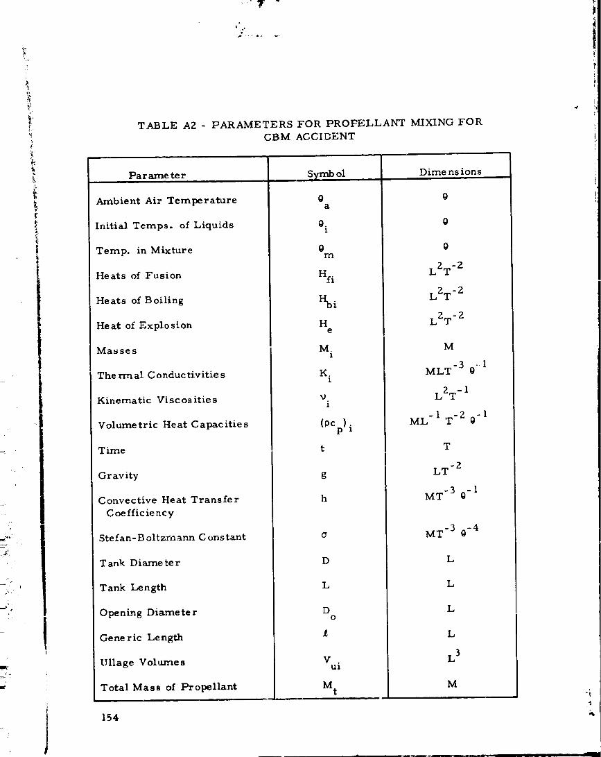
9
t
TABLE AZ - PARAMETERS FOR PROPELLANT MIXING FOR
CBM ACCIDENT
Par anae te r
Ambient Air Temperature
Initial Temps. of Liquids
Temp. in Mixture
Heats of Fusion
Heats of Boiling
Heat of Explosion
Masses
The rrnal C onduc tivities
Kinematic Viscosities
Volumetric Heat Capacities
Time
G rav ity
Convective Heat Transfer
C oe fficiency
Stefan- Bolt zrn ann Cons tant
Tank Diameter
Tank Length
Opening Diameter
Generic Length
Ullage Volumes
Total Mass of Propellant
S_nb ol
Oa
Q.l
0m
Hfi
He
M.l
K.1
Vi
(0Cp) i
t
g
h
0
D
L
Do
Vui
M t
Dime ns ions
@
0
0
LZT -z
LZT -z
LZT -2
M
-3 -.lMLT O
LZT -I
-I -2 -IML T 0
T
-ZLT
MT-3 Q-1
MT-3 0-4
L
L
L
L
L 3
M
154

i:
TABLE A3 - DIMENSIONLESS GROUPS FOR PROPELLANT
MIXING FOR CBM ACCIDENT
Term No.
TT1
13"
2
rT
3
13"
4
TT
5
n6
rt7
"9
nl0
II
Ii
T_13
n14
1"t]5
13"16
Hfi I gL
Hbi/gL
n /gLe
D/L
D /LO
_/L
V .iL-ul
Mi/M t
llZlLII ztg
(OCp) i v./K.l 1
hL/K.1
v IL 31z IIz• gI
_9 3 3 L 2g /K.a 1
K. L 1/2 01.
312.a/Mt g
Description
Tempe rature Ratios
Enex gy Ratios
Length Ratios
Volume Rat_ os
Mass Ratios
Sc ale d Tim
Prandtl No.
Nusseit No.
Pseudo Reynolds No.
Ratio of Radiation to
C onduc tion
Ratio of Conduction tc
Ine rtia
155

• .,_ " q,j•
These are rr6 _. , rr8, _ and TT Employing these restrictions, the re-' 7 9 I0"maining rT terms require he following interrelations between scale factors.
o
t.
_Z _ XO = 1m
TT3' _4' TT5 _ 1 =k L
._ ----_k "), I/2II t L
rr ---_k ), =I13 h L
A quick examination will show that these interrelations can only be satisfied if
all scale factors, including the length scale factor XL, are u_.ni_. That is,
no sub-scale model is possible which correctly scales all of the phenomena
which were initially assumed tube important! This impasse is not unusual
in attempting to model complex phenomena. One must now consider those
effects which will hopefully be of minor i,rlportance, and let them, deliberately
go out of scale.
For the problem we are considering, radiation heat transfer to the
outside a_-nosphert can perhaps be safely neglected, becaase the mixture is
cgnfined within the tank up to the time of interest. So, let us ignore term
rT15 . For the mixing fluids, conduction and convection are probably theprimary modes of heat transfer, so we wisi-, to retain _13' Nusselt No., be-
cause this term is a ratio of these two effects. Inertia effects are undoubtedly
important and should be retained. Gravity is triply important because it
affects mixing impact conditions, convection, and bubble migration. Whether
viscosity is important is not certain. We will assume that it is not, and ignore
rT14 . Heat_ of fusion, boiling and explosion appear to be important, so weand rT This reduced form of the law can be w,itten:
should retain u 3, 4 5"
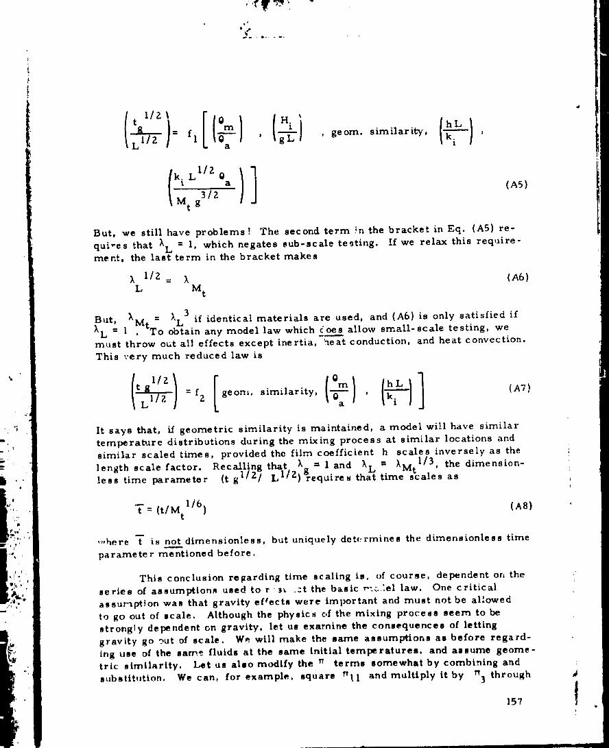
Qo
'¢
I °Ll/2I; , geom. similarity,
ki L IIZ 0 (AS)
But, we stillhave problems ! The second term ;n the bracket in Eq. (A5) re-
qui-es that XL = l, which negates sub-scale testing. If we relax this require-
sent, the last term in the bracket makes
X l/Z__ X (A6)
L M t
But, X = ),L3 if identical materials are used, and (A6) is only satisfied if
XL = l .MtTo obtain any model law which __oe__=_sallow sma11-scale testing, we
must throw out all effects except inertia, _eat conduction, and heat convection.
This very much reduced law is
t g = f2 geom. similarity, ,LI/Z
(AV)
It says that, if geometric similarity is maintained, a modelwillhave similar
temperab_re distributions during the mixing process at similar locations and
similar scaled times, provided thc film coefficient h scales inversely as the
length scale factor. Rec_lling that kg = I and XL -- XMt- I/3, the dimension-
less time parameter (t gllZl L l/z) requires that time scales as
T = (t/Mt I/6) (A8)
,,,here T is not dimensionless, but uniquely det¢:rmines the dimensionless time
parameter mentioned before.
This conclusion re_arding time scaling is, of course, dependent on the
series of assum_ion_ used to r m_ _:t the basic r:_:el law. One critical
assur_ptlon was that gravity efCects were important and must not be allowed
to go out of scale. Although the physics of the mixing process seem to be
strongly dependent on gravity, let us examine the consequences of letting
gravity go out of scale. We will make the same assumptions as before regard-
ing use of the same fluids at the same initial temperatures, and assume geome-trlc similarity. Let as also modify the _ terms somewhat by combining and
substit_Jtion. We can, for example, square "ll and multiply it by _3 through
157
#
J
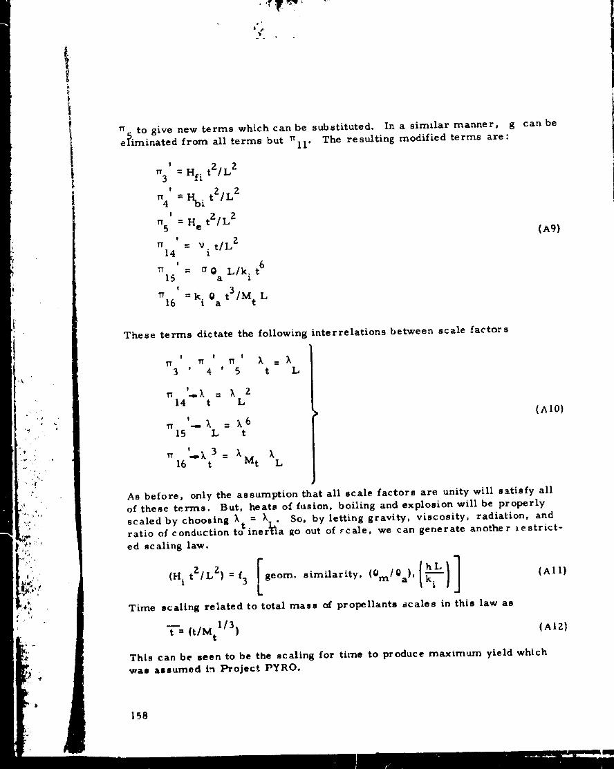
t
!!
'4
77_ to give new terms which can be substituted. In a similar manner, g
e_irninated from all terms but 7711" The resulting modified terms are:
77 '
3 = Hfi t2/L2
!
774 - Hbi tZ/LZ!
rr5 = H e t2/L 2
' /L 277 = _. t14 x
' t 6,_ = 0 @ L/R.15 a *
' t 3/M t77 =k. 0 L16 t a
can be
(A9)
r
J
4
,,t
,i
°.
b ,
These terms dictate the following interrelations between scale factors
, ! , )_. _ 77 ). =3 ' 4 ' 5 t L
__), = ), 214 t L
TT
77
'-.X =),615 L t
1..k 3 = ), k16 t Mt L
(Al0)
As before, only the assumption that all scale factors are unity will satisfy all
of these terms. But, heats of fusion, boiling and explosion will be properly
scaled by choosing X - ), . So, by le_ing gravity, viscosity, radiation, andratio of conduction totiner_a go out of.cale, we can generate another xestrict-
ed scaling law.
(Hi tZ/L2) = f3 geom. similarity, (0m/0a), k-q-"
Time scaling related to total mass of propellants scales in this law as
I/3)"_"= (t/M t
(All)
(AIZ)
This can be seen to be the scaling for time to produce maximum yield which
was assumed in Project PYRO.
158
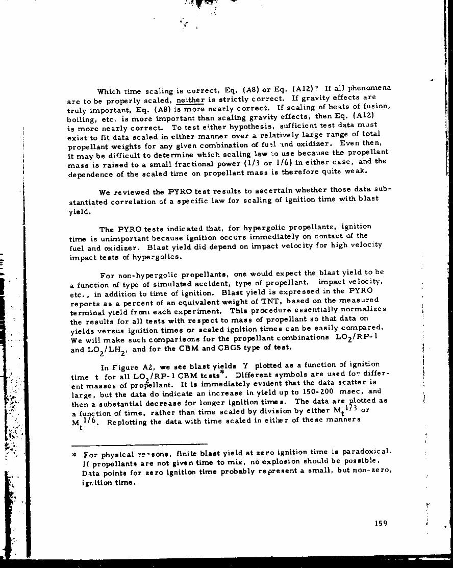
L
/
Which time scaling is correct, Eq. (A8) or Eq. (AIZ)? If all phenomena
are to be properly scaled, neither is strictly correct. If gravity effects are
truly important, Eq. (A8) is more nearly correct. If scaling of heats of fusion,
boiling, etc. is more important than scaling gravity effects, then Eq. (A12)
is more nearly correct. To test e_ther hypothesis, sufficient test data must
exist to fit data scaled in either manner over a relatively large range of total
propellant weights for any given combination of fu_l _nd oxidizer. Even then,
it may be difficult to determine which scaling law _.o use because the propellant
mass is raised to a smallfractional power (1/3 or I/6) in either case, and the
dependence of the scaled time on propellant mass is therefore quite weak.
We reviewed the PYRO test results to ascertain whether those data sub-
stantiated correlation of a specific law for scaling of ignition time with blast
yield.
The PYRO tests indicated that, for hypergolic propellants, ignition
time is unimportant because ignition occurs immediately on contact of the
fuel and oxidizer. Blast yield did depend on impact velocity for high velocity
impact tests of hypergo]ics.
For non-hypergolic propellants, one would expect the blast yield to be
a function of type of simulated accident, type of propellant, impact velocity,
etc. , in addition to time of ignition. Blast yield is expressed in the PYRO
reports as a percent of an equivalent weight of TNT, based on the measured
terminaIyield fr_nl each experiment. This procedure essentially normalizes
the results for all tests with respect to mass of propellant so that data on
yields versus ignition times or scaled ignition times can be easily compared.
We will make such comparisons for the propellant combinations LOz/RP-I
and LOz/LH Z, and for the CBM and CBGS type of test.
In Figure AZ, we see blast yields "{ plotted as a function of ignition
time t for all LO2/RP-1 CBIVi tests =. Different symbols are used fo" differ-ent masses of propellant. It is immediately evident that the data scatter is
large, but the data do indicate an increase in yield up to 150-200 msec, and
then a substantial decrease for longer ignition time s. The data are plotted as
a function of time, rather than time scaled by division by either Mtl/3 or
Mtl/6. Replotting the data with time scaled in eitI_er of these manners
For physical re-sons, finite blast yield at zero ignition time is paradoxical.
If propellants are not given time to mix, no explosion should be possible.
Data points for zero ignition time probably represent a small, but non-zero,
igr:ition time.
159

4"
t
|
1I
tl "
,-r
!
,t
0 <]+0
0
0
160
0
0
0
'A
0
0131A
O
<1
O
O
OoO
O
O
<1
O
or}
D
I
c_
O
ZOI,-4
b_
O
o,]
produces no less data _ca_er than is already present. Figure A3 shows a
similar plot for LO2/LH 2 CBM tests. Again, the scatter is considerable,but a trend to increasing yield with increasing time is evident, with no appar-
ent decrease at long times. One isolated data point with a high yield may
indicate peaking at near 200 msec, but this is inconclusive. Again, replotting
on scaled time based doesn't improve the scatter.
Data for all LOz/RP-1 CBGS tests are plotted in Figure A4. It is evi-
dent that impact velocity for this propellant and type of test does have a sig-
nificant effect on blast yield, and that yield increases for a maximum and
then decreases. The same trends are evident in the data for LOz/LH 2 CBGS
tests plotted in Figure AS. Some type of normalization of yield versus impac _-
velocity would undoubtedly reduce the scatter evident in these two figures, but
the sprea_i would still be great. As for the CBM tests, there is no evidence
that scaling ignition time would decrease the data ._catter.
We draw different conclusions from this study of the PYRO blast data
than do the authors of that study. They concluded that, for all but the LO_/
RP- I CBM tests, explosive yields scaled as a function "t" = (t/Mtl/3). Wez
conclude, on the other hand, that the data do not verify any particular scaling
for ignition time. The blast yield ;.s certainly a function of ignition time and
that function can perhaps be estimated from _,he PYRO data fnr specific pro-
pellants and types of test. Direct plots of yield versus ignition time appear to
be as valid as plots versus (t/Iv[tl/_), (t/iM%I/6), or perhaps any other scaling
involvin_ a small fractional power of M t.
)
161

i
16Z
oO
O
<10
o<1+
r,/)
[,,,I
UN
,-1N
O,,,,]
=E oellll
,-II-,
fe_
0

0
n
<] <I00
0<]
+ 00
n
0
0
OO 0
eO
0
IQ 8 _ @ @
N
$ 'A Q131h 163
©_Q(J
,.j
N
0,J
l-d
I,,,4
Z0
_4
,Jl.d
<
Id0_
L3i-.I
b.,
i
!
'i
I
i

'A Q'I31A o
164
.d'
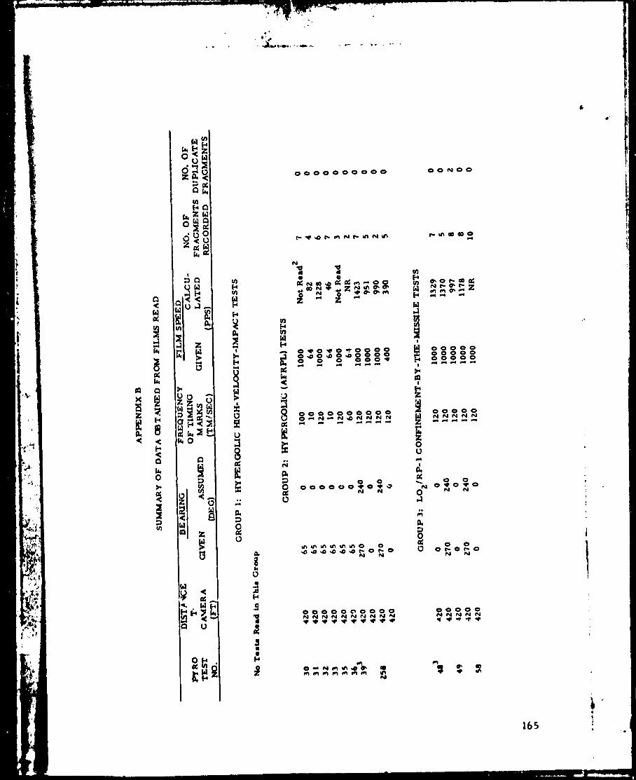
• Ss_-
0000000000OONO0
iq
_i _ Z " Z "_1o ._ _
' i i! o.o.o ooooooooo0_00 _00,,0000 O 00000
0 0 0 000 _'_ 00000
_ _ 0000000000 00000
0 00 I',, 0 _ 0
r.i /NI _'4 r4 N9999999 _P 9 _P I 9 _' "P 9
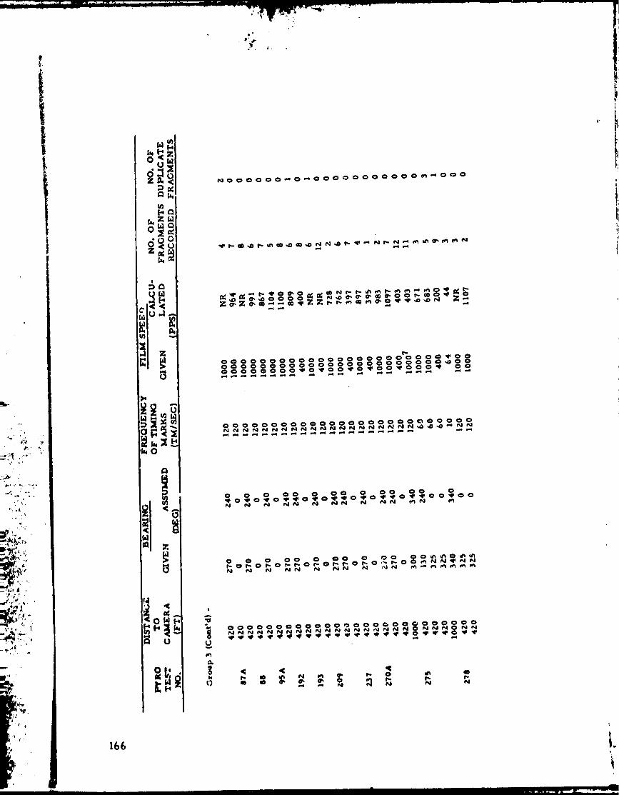
t
la ml
NO00000_0_00000000000 _ 000
oo _o_o__
!
166

,_r_
• 'd
f
!,
J* _[_1 0 0 0 0 0 0 0 0 0 0 0 0 0 0 0 0 0 0 0 0 0 0 0 0 0
V)
(n
k-4
<
0
I
o : ! ooooooo° oooo=oo , o_=o_o_o_o=o_o_oo=
Lu_ ur_ u'_ o * 0 i,, 0 r.. 0 T.- 0 I"- 0 f'- 0 r" 0 ¢_ r"N N N * 0 0 , 0 t_ _1_I . _ N _1 N N N
_ i_ i_ i_ _1_
-'_0 0 0 0 0 0 _ 0 0 0 0 0 0 0 0 0 0 0 0 0 0 0 0 0
167
_r
i .
[4 {/1
: I_, ,¢
U)[-*_1;[ [_1
Z
a
0000 _
00000QO000
00000
0O_l*O
e*J
lOll
'i Q t
M
0 O0000_ 0 O0 O0
0
_(_ O0 _ _1'_'_"*
2:
0
0I
!
!
0U
N
0
0
0
0 0 00,'_ 0 0q* 0 q_ 0 _IP -._ qL' 00 q' 0N N N_IN N N
! I I I !" 00 I _ I
I I I I I I N N I I
N N_ N I
M[-,
[-,
!
8
Q
N0
0
0
D,
0k
0
e
QX
168
7
I
,I
I
io
o_!_
4
0
Z
U
o__o_
_ 00000000000000000000 _00000
[_
!
I
Z
Z
Z0
N
0
0
0
,_:___
0 O00000 O000 O000000 O00000000
0 0 O0 0 0 0 0 0 0 O00_0_0_00_0_0_0_00_00_0_0
I ! I ! IoOoOoOOooOo:o_o_ooOoo , ,, ,,, ,,, ,,, ; , ', , ',
0 _ hi e'_ _ _'_ .*0 _'* 0 "=* _'_P _D _l
169

7
r
| *
! t
b.] t/Y
u'JF_r_Z_
_Q
i
_o
o
z
u
O00000 QO 0000 NO000
_zzzz$_$$_2_zN_
0000000000000000_00000000000000_0_0_0_0_0_0_0_00_
00000_00000000000
0 0 0"0 0 0 O_ O0
0 0 0 _ 0 0 00_00
!
r_
.3
0 _ _ 0 N _ ur_ 0',
,,=, _11 N N N N N
u_
u[-4
M¢.,)
r_
Z
o
I
;=MZ
o1.9
N
N
o
;30=;L_
00000000
__0_0
__o__zz__
O0000it_NNNNIIli
OOOO_¢IsNNNNII I
0 0 _ '="
170

t
+.
,},+...31:1.31
+.
O00_O000000000000000000000000
o_o_o_o_o_o_o_o_oo_o_,o_o_ o
o oo o o o o o , :oOoOo8: ', : ', :op.,o_o_op.,op...o_o_o : , ,,., +.,, , , , , ,
!
- + + ++ +++ om+mm|:::,,,,o _ _g : 1_+ ++ , , , , ,+++::+ o .+ ,,II m
171
'¢
ITZ
v •
_Z_I.
!
_G
Z
u
Z
000000 000000
ill
_ mo
N
0 _
H
0 0
Jo
i I i I I I
it O O 0 I I ' o o I0 !'.- o o I'.- 0 * o t I o
o o _1
gl,
1"_3

?',
.J
174

APPEN DIX C
MODEL ANALYSES FOR FRAGMENT VELOCITIES, RANGE, ETC.,
FOR BURSTING LIQUID PROPELLANT VESSELS
In an attempt to facilitate comparisons of the data which have been un-
earthed during this study, let us conduct s_veral limited modq, l analyses re-
Sating to various aspects of the problem. To avoid too complex model laws,
we will divide the problems into several subproblems.
Initial Velocities for CBM Case
Consider first the bursting and acceleration of ves_el fragments by an
internal explosion (CBM case). A list of physical parameters appropriate to
this case and part of the problem are glven in Table Cl, Nith dimensions in a
Force-Length-Time (FLT) system. The twenty-one parameters in Table CI
can be combined into eighteen dimensionless group,, (Pi terms) by the methods
of dimenslon_l analysis. One such grouping is given in Table CZ. based on
mass of propellant, heat of explosion _f propellant, and a characteristic length
as repeating variables. Table CZ includes descriptions of the pi terms.
The dependent variables in Table CZ are essentially _!3' _14' "I:, and
/W hr°ugh 5_'17' Terms _ r, are mass or density rat'os, 6nd terms-_ thro,_,¢h
nll require i_¢(_u etric similarity. Term _IZ dictates scaling of energy re-lease, and ;s e, _Ivalent to fractional bl_st yield y. Term _15 can be c¢,nsid-
ered as a r,stio of ve_se] burst Gressur_ Pv to the pressure which would be
generated by contained reaction of all of the mass of propellant. Finally, _18
requires Identlca _, equation of state for the reactir_n productions of the explod-
In_ propellant,
The mo,lel law in Table CZ c-n be expressed in functi¢_nal form as
• l[ Iil n/z) { ,x,31M in) (thinlY/:')' ".JL f _ ' t P. ' •
= [ [')ellsity ratios, Geom, SLIT., (E/N4t|le_,
"e'(pvL3/Mt H} ' x -Ij (r;I)
If we confine f)ur comparisons to tests with Meometricallv nimil_r tanks madeof the same materials and filled with the same propellant mixt_res, then the
density ratio terms .nd terms descrlbinll lleometric similarity will all be th_
: 17_
d_ t
Symbol [
Iv
M t
Mr
He
D
[,
Do
V
0P
V
Mf
Af
Uf
VV
v1,1
t
P_,
176
TABLE CO - PHY_CAL PARAMETERS FOR VESSEL BURSTBY INTERNAL EXPLOSION
Dtmenelono
FTZL . I
FT2L- l
FT2L- l
FL
LZT -2
L
L
L
L
FT2L "4
F,rZL -4
FTZL - '
I
t,
,ILoT
L 1
t.
FL "L
T
.tFt.,
,m
Parameter
Total mass of vessel
Total mass of propellant
Reactlve mass of propellant
Energy releaoe during ex-
plosion (blast yield)
Heat of ex_.ios|on of pro-
peilant mixture
Tank d_amete r
Tank lenlth
Diameter of internal bulk-
head rupture area
Thickness of vessel material
Density of propellant
Density of vessel mater,at
Number of fralmento
Mass of Individual fralur, ents
Mean presented area ,)f Indl-vldual fraeme.t s
Velocity ,,f Individual frail-merit
Internal volume -f tank
Ulla|e volume nl' tank
Ratio of 0per,lie heats ",,-
esplosinn products
Praetors within tank durtn|
eeplollon
Time
_urot preooure of veseel

_o
TABLE CZ - DIMENSIONLESS GROUPS FOR VESSEL BURST
BY INTERNAL EXPLOSION
TeFm
M /M 1v t
Mr/M t
Mf/M t
0p L3/Mt
0v L3/Mt
D /L0
h ILV
Af/L z
v IL 3U
V Ih 3v
E /M t H e
U flH_ 'Z
p I,3/M tH e
PvL3/Mt lio !tHl/Zl_
e
Description
M_,*s or density ratios
Geometr_(, slmils rity
Energy scaling
Velocity scallnK
Pressure ,callng
Time scaling
Number of fraRments
RAtio of specific h, ats
177
1
!
i
..... _ s._,._,_qlL
o
3 and_ will not change. Also, the burstsame independent of scale, )'I., = )'Mt'
pressures Pv for geometrically similar vessels of the same material are iden-
tical ()`Pv - 1). Because we are using the same propellant, )'He = 1. Under
these restricted conditions, Equation CI reduces to**
uf, p, (t/L), n] - f(y) (cz)
In other wordi, Equation (C 2-) says that initial fragment velocity, pressure rise
within tank prior to rupture, time scaled proportional to length, and number of
fragmenti get.stated should all be fLnctlons of fractional yield.
Many other interpretations can be made of this law. If we do not make
the Iimplifying aisumptlonI above, then we nr.ay be able to compare s ,me test
results for different propellanti. Terms _12 and _]3 can be combined to form:
, z /E (c3)_12 = UfMt
which -an replace _12 in Equation (CI).
This term defines an equivalent dimenIional group
G' -" U_W /Y (C4)IZ t
where W t iS total weight of propellant and Y is blast yield in percent. Wehave recorded most of our fragmentation data in terms of these quantities, and
/
so can plot GIZ , or Its square root, versus Y (equivalent to _12 ) or against
"15' provided we use a coniistent let of units. It is quite likely_hat _ is onlyweakly dependent on type of propellant, _o perl_pi we c_n I_nore it. The
model law does point out that (L',/L) and (D/D o ) are p,,tent_ally important geo-metric r_tloi, and thac mean fragment area may icale as the square of the
length scale.
Initial Velocities for CBG5 and llVl Cases
In this caie, the propel[anti ipill, mix on the ground, and then ignite
o." the missile Itnpacts the ground at hish velocity. Solid objects and nearby
*The iyr,_bol _ denotes a scali factor, and a subscript letter deno'_en th_
pKysical parameter belng scaled._,WNo'e that these prodtlcti are not now n'ondimeniional, because we have
de|sted dlmeniiona| tsrmi which do not c'nanqe.
appurtenances are then acce1.erated by the resultant blast wave to some maxi-
mum velocity ("initial" velocity). The pertinent physical parameters are some-what different than for the CBlvi case. Geometry of the vessel is no longer im-
portant, but kravlty and impact velocity must be considered. A list is given in
Table C3. Again using as repeating variables Ivlt, H e and L, we obtain a group
of fifteenpt terms ft.om the eighteen physical parameters. These are given in
Table C4.
Many of the terms In Table C4 can be seen to be identical to those in
Table Ca. These include the mass ratios _I through_3, area ratio_4, volume
ratio "7' scaling for fragment velocltY_9, energy scaling _I0, pressure scat-
tog _12' tlme ecali,_g _14' and number of fragments "15' The terms which are
new are "5' "6' "8' _II' and-l., and some terms in Table CZ do not appear.This model law can be expre0eec_&s:
[ (Ufl/H_/Z)' (pL'3/MtHe)' (qL3/MtHe _' (tHl/_-/L'_}'e(Afl/LZ)' n_
• f [Density ratios, Geom. elm (E/MtHe_ CD_ CUt/HI/z)• I | | e _ D
L/He ) ] (C5)
The term,lt, If strictly adhered to during tests of the same propellant, wouldprevent comparison oftestJ conducted at different geometrlc scales, because
X_ = I, )'He = I, and therefore )'L = I.
If we deliberately let this term go out of scale, which Is equivalent to
ignoring g,avity effects, then almost the same model law as for the CBM case
results, with the addition of a r_quirement of scaling of impact velocity from
"8' If we assume that we cannot i|nore effect of gravity o;_ such physical pro-ceesee as spreading and Intermingling of the fuel and oxidiser after spilt, ini-
tial trajectory of fragments, etc., then Equation (C5) requires a change in heat
of explosion H e in order to change length scale. It is suggested that we simply
try plottin 8 fragment velocities from CBGS data versus blast yield for the same
propellant. We know from the PYI_O work that blast yield is a function of im-
pact vsto,.Ity V i, so term "8 may oe already accommodated by metsuring
blast yield. An alternative might be to plot the term
I
"9 " vtt/'rw'-' (c6)
,,ereue blast yield for the oam_ propel'ant.
that gravity effects were indeed tmpor.ant.
Correlation here would indicat_
f
179
_o
TABLE C3 - PHYSICAL PARAMETERS FOR FRAGMENT ACCELERATION
AFTER SPII, L AND EXPLOSION
'o #._J
' 11 \
r •I,
¢ 7 ¸
.fB
Symbol Dimensions
M FTZL'Iv
Mt FT_L "I
M FT'L" 1r
l'[fi FT2L - 1
E FL
H LZT'Ze
L 3VP
-I
Ul LT
g LT -2
L i -'-
L L
L 2AlL
-ILT
Ufl
C _..
Di
p FL "2
-2q FL
t T
Para_ne tern
Total mass of vessel
Total mass of propellant
Reactive mass of propellant
Mass of the solid body or
appurtenance
Energy release during explosion
Heat of explosion of propellant
Volume of propellant
Impact velocity
Acceleration of gravity
Length ratlol
Characteristic length
Number of fragments
Mean presented area of [th solid
body or appurtenance
Velocity of same
Drag coeflicient of same
Overpressure in blast wave
Dynamic pressure in blast wave
Time
180
e'
0 •
Number
1
"Z
rt 3
"4
"5
6
"7
"8
"0
"I0
II
I"TIZ
TI13
14
15
TABLE C4 - DIMENSIONLESS GROUPS FOR FRAGMENT
ACCELERATION AFTER SPILL
Te rm
My /Mt _I
• /M t
Mfi/]_ _
Afi/LZ£1 1
CDl
V /L 3P
l/ZUII/H e
E/M t H e
gL/He
P /MtH e
L 3q / M t 14e
tH !/_/Le
n
Descri tion
Mass ratios
Geometry
Drag coefficient
Volume ratio
Velocity scal!.ng
Energy scaling
Gravity scaling ,
Preslure s-.aling
Tinle scaling
Number of fraRments
i
181
f
q-
Trajectories of Fragments in Free Flight
After the fragments have been accelerated to their maximum velocities,
then the problem is one of exterior ballistics for each fragment. Most of the
parameters governing the resulting trajectories differ from those in the previ-
ous problems. They are listed in Table C5, and a possible set of pi terms is
given in Table C6.
The first four pi terms in Table C6 are initial conditions, _sand _6
are aerodynamic coefficients, and _4 through _I0 specify geometric similarity.
Term rTq canalso be considered as the dependent variable. Term _iI specifies
gravity scaling, which is essential in trajectory problems and cannot be ignored.
Terms _12 and _13 are wind velocity and air density scaling, respectively. Tim
model law can be written as:
(Rf/L) =fE(Uft/L) , {Wft), ef, Tf, CDf, CLf, (Af]LZ)' _xif/L)' £''1
(gtz/L), ('Uwt/L.), (oaL,3/Mf) ] ((;7)
From our physical knowledge of exterior ballistics and the problem of frag-
ment scatter, we can considerably reduce this function space. Range may be
dep_!_ndent on azimuth angle T and scaled wind velocity (Uwt/L), but this depen-
deft is weak for high velocity and "chunky" fragments. Furthermore, our data
from missile maps average ranges over all azimuths, so this dependence is
not considered. The "liftint" characteristics of the fragments are represented
by,CLf and by initial spin wft. Again, these characteristics represent randomana uncontrolled quantities which we cant_ot assess, so we again ignore them.
A reduced form for Equation (C7) is then
(Rf/L,) :f[(Uft/L) el, C ('Af/L'z) (=if/L)' *i' _ tz/L)'' Df' '
(OaLl/Mf) ] (C8)
Of these remaining parameters, the first two _ ad the fifth are scaled initial
conditions. The dAag coefficient is a functior. '.." _Af/L _) and £i and is there-
fore superfl,_ous. So, for l ragments of simil,xr f;eometry and s_.me scaled
initial con_.ttons, the law iurther leduces to
Symbol
Uf
tOf
CDf
C Lf
Af
Mf
6f
X..
Rf
g
oa
!
U%W
t
L
TABLE C5 - PHYSICAL PARAMETERS FOR
FRAGMENT TRAJECTORIES
Dimensions
-1LT
-lT
Parameter
Initial linear velocity
Initial angular velocity
L z
FTZL "1
L
L
-ZLT
FTZL -4
-1AT
T
L
Drag coefficient
Lift coefficient
Mean presented area
Mass of fragment
Initial elevation angle
Initial azimuth angle
Initial coordinates of
fragment
Range of fragment
Acceleration of gravity
Density of air
Length ratios
Wind velocity
Time
A characteristic length
183
i
Number
1
_2
_3
_4
_5
"6
_7
_8
_9
l0
TTII
_lZ
rT13
TABLE C6 - DIMENSIONLESS GROUPS FOR
FRAGMENT TRAJECTORIES
Term
Uft/L 1
f
Of
_f
CDf
CLf
Af/L 2
xif/L
Rf/L
1
gt2/L
U t/LW
L 3Oa /M{
I
De scription .
Initial Conditions
Aerodynamic Coefficients
Geometric Similarity
Gravity Scaling
Velocity Scaling
Density Scaling
184
e j
Now, because kg = 1, r_ll requires that
xz (ct = ki,
The first term in Equation (C9) then reqaires that
= k L .Uf
or
. 1/2_ (C11)
XUf = _L '
i.e., initial velocities should scale as the square root of the length scale for
the same scaled range. The third term is automatic%11y sat;qfied because
)'Qa = I and "_,L3 = kMf.
We can combine _7 and _13 to form
, z/3 (c,z)_7 = Af 0a /M
= 1, a dimensional form of this term isBecause )_Oa
G 7 = Af/W /3 (el3)
where Wf is weight of .(ragment.
This may provide a rational grouping for ulotting versus scaled range•
APPENDIX D
COMPUTER PROGRAM ENTITLED /W2/ IN FOKTRAN IV
Function: This program computes initial fragment velocity.
Given the following input data:
A) Characteristics of some explosive fuel-oxidizer gas mixture at moment
t = 0 of detonation.
(CAP1) Ratio of specific heats, R
(A(_) Speed of sound in medium in in./sec
(_) Initial pressure in psi
B) Characteristics of containing vessel
(RR) Internal radius of,,essel + unburned fuel in inches
(TM) Mass of vessel .+ unburned fuel in Ib/secZ/in.
(FN) No. of fragments
C ) Calculatory requirements
(AH) Time interval of each calculation in seconds
(XMAX) Maximum time to last calculation in seconds
Variables: The definition and units of the vari les in this program are _ive'
in the following table.
TABLE (D- 1)
ProgramVariable Variable Definition
FF F projected fragment area
CAPI _ specific heat ratio for explosive
mixture
AO a0
speed of sound in explosive pr,_ucts
mixture
Units
2i,1.
none
in/sec
186

'¢
1
)
,i
Program
Variable
PO
FN
RR
TM
FK
AH
XMAX
FNI
FNZ
FN3
GI
GZ
G3
G4
T1
JJ
PI
CAPZ
C A P3
C AP4
XX
Variable
POO
n
R
M t
Uf
Definition
initial pressure after explosion
number of _.'ragments
radius of explosive products mixture
,nass of shell + unexploded fuel
c oefficient
time interval
max imum time
if < I displays T-NORM (;, G'
if
if
distance to initial velocity
, (_,1
< I displays normal pre _sure + tinxem
< 1 calculates maximum range
Units
psi
None
in.
Ib- inZ /se c
none
sec
sea
none
nole
initial fragment velocity
none
in.
ft/sec
Z
initial fragment acceleration in/sec
final explosive product mixture pressure psi
time to initial velocity sec
counting variable s none
the constant _ none
the quantity (I- x)/_. none
the quantity - 1/)t none
the quantity (3)t. 1)/Z)t none
displacement normalization coefficient
(see Eq. -35} in.
,,7

•,_,E_._w-k,
ProgramVariable
THETA
A1
BI
c_
X
Y(Z)
Y(3)
y(l)
NA
F(I}, F(Z),
F(3)
TT
PS
Var lab le
8
Definition
time normalization coefficient
(see Eq. .35)
the coefficient ¢z (Eq. - 36)
the coefficient 8(Eq. -_6)
normalized initial fragment displace-
ment from center of sphere
normali.",e d time
normalized veloc ity
normalized pressure
normalized fragment dis placement
number of differential equations to
be solved
differential equations solved (see
Eqs. .34and -36_
normalized time
normalized pressure
Units
sec
none
none
none
none
none
none
none
none
non_
none
The subprogram entitled {RUNGE) is described in the following:
188
FORTRAN IV
RUNGE - KUTTA
FILE NAME:
SUBROUTINE NAME:
PURPOSE:
METHOD:
ARGUMLNTS:
FI$
RUNGE
This subroutine employs the Fourth Order Runge Kutta Method
to solve. N simultaneous first-order ordinary differential equa-
tions by calculating successive values of Y according to the
formula:
hYi+l" Yi ÷ 6 (Ki + 2K 2+ 2K 3 ÷ K 4)
where K I • f(X i, Yl)
K 2- f(Xl +h. yi+-_)
K s" f(xi÷2' Yi + )
K 4 • f(x i + h, Yl + hK3)
The subroutine is called by the calling program five times in
order to approximate successive Y(l)'s; tl':efirst time to initialize,
the second time to calculate KI(I), the third time to calculate
K211) , the fo_rthtime to calculate K3{[ _ and the fifth tlme to cat-curate K4(I). In addition, each time the subroutine is called, itca]culates a new Y(1) and anew X(i) which are _ returned to :he
calling program where the functions (first-order differential
equations) are evaluated with the new X(1) and Y{I). These values
of the function are then returned to the subroutine where they"are
used as Kl(1). K2(1), K3(1), or K4(1) and appropriately accumu-
lated to obtaln Yi+l(1) in the 5 calls to the subroutit_e.
The _ubroutlne _.UNGE uses nine argn_ments: _, "I, F, X. H, 'Vl,
SAVEY, PHI, K
I. The first argument, N, represents the number of simulta-neous first-order ordina:'y differentlai equations to be ,qolved.
The second srlument, Y, is the array name which the calling
prolram uses to tran_mlt the initial Y(1) values for eachdifferential equation. Upon completion of the 5 calls toRUNGE, Y(1) will contain the new approximated values for
the Yi+l(1)'s.
'¢
LIMITATIONSAND
COM ?,tENTS:
190
9. Tks third arl_meut. F. is the array which coo.tains the cur-rent values d the differential equaticms calc'-_ated by t.he
main program, i.o., F(J) contains the value ot the jm first-order dlfferential equatlou.
4. The fourth ar_ment, X. represents the independent variablewhich should be initialized in the main program before calling
RUNGE. I_UNGE increments X by the stepsize H.
$. The fifth ara_ment, H. represents the step size for X.
S. The sixth arlumcnt. M, indicates which of the five passesthe subroutine is to be executed. The main program must
initialize this argument as I. RUNGE ti_en successively
mcrements the variable by ! up to 5.
7. The seventh argument. SAVEY, is used within RUNGE and
n,,_st be d/mensior_d in the calling program to be of zlze N.
$. The eighth argument, PHI, i,., also used internally by RUNGE,but must be dimensioned in the calling program to be of size
N.
9. T_e ninth ar_ment, K0 is manipulated wlthin R_,'NGE. K
should be teste_ right after the calf _o RUNGE, in the calling
program.
When K=I, control should transfer to a set of code in the
calling program which c,_Iculates new values fox" the flrat _
order differential equations, F(1), with the current valuesof X and Y(1). Then RUNGE should be called again.
When K-2, the approximation for Y{I) is completed. Values
for the Yi+l(1)'s are -tored in Y(I] at this time. and normalflow of the calling program should resume.
I. The calling ?rogram must dimension SAVEY and PHI.
2. The calling program must set M-I before calling I_UNGE.
3. The calllng program must set up the N first-order differen-
U&i equation values in an _rray F to _e pass_'d through toRUNGE whe_ the subroutine returns with K=I.
4. The calling program must set up separate arrays if all X andY values for the set of differential equat|ons are to be sav_d.
perhaps for plotting puv. poses.
/,
PROGRAM /WZ/ LISTING
DIHENSIEN F(3),Y(3),"/I (3), ''I'_-(3)•PS(50)•TT(50)
30',) F(_RHAT (_/, 20H READ IN TRAJ. AI'IGLE)
390! F_RHAT (EI_).3)301 FORMAT (2/,35H READ IN DRAG COEF. AND AIR DENSITY)
'3011 FgRHAT (2I-:10.3)302 F@RMAT (_/,,9,8H REAl) IH F._A'3MEHT MASS CgEF.)303 FgRMAT (z;/`,25H CONUITIO_JS 3N T._JECT_RY)304 FORHAT (/•RIH A;.IBIENT AIR DENSITY-,EIO.3,,|7H LBS./CUBIC FT.)
305 FOR"tAT (/•16H AIR" DRAG COEF.=,EIO.3)306 FOR;dAT (/21r! FRAGHEMT HASS CggF.=,E IO.3)
307 F._t.IAT (/,IL;H TP,AJECTORY AHSLE,,,,EIO.3,.'_I'L DEGREES)
3071 F99."I_T (3/`,qH CIIECK C=,EI0 .3)308 FOP,"I_T (3/,L5H HAXI_'.IUH RA,IGE=•EI<?o3,/_iI FT.)309 Fg,RI:_.r (RI`,45H READ IN <_PPA, S.J!.I_JDSPEED• INITIOA, PRESSURE)
310 FORinT (3EI0.5)311 F',IRM_ r (')./,78H REAU IN :J_. OF FRI_G'IENT.5, RADIUS 0F EXPL.,
_"b_S 9F ::_IYI,L-FUEI.• DISC;IA.'_G': C ;_EF*)
312 F0IB.HA; t,_EIO._)
313 FOR:4A" ('/, _6H READ IN TI_IF IHTE!O/:_L, '.I,__,IHUH TIHK)
31a FSR'If_T (2£I:).3)315 FORHAT (3/, _.:)H GAS CH_'rIACTF.IISTICS•/•7.1 .(App/_=`,Itl0.3•
I,=H S2UNi_ -.°FEl_=`,ElC).5_'7H I!I/5EC,/,IOH :J_E,_SURE ,glO.3,_H PSI,,
2/,231i UES-;_;L C:{_I_CT-:RISTICS./• _i! p_ADIUS=,LIO.3,5H INS,,
P_H _IASG=•.:.IO.._•I7H ".r_S.-_d.C.=_./IN•/, 1_:: "_* 3F FRAGHE ;dTS='r'lO'3";':/)
316 Fr4RH_ T (2/,3.),-, ,:_I._PLA'." DY;},t i_; U_I_{.? Y:'S=I :_]_=_-)
31'7 FORHAT (2/,3),H DI:APL,"_Y :13i_;1. PP.E:;S.? /'_::_:=1 XI'_=_.)
318 F_ARH.qT (2/•3_.i IAK!.: .{;_t'JGE C_d,C'JL;_TI3",'? Y/,S:'I NO=2)319 F_RHAT (3/, I 31 FINiaL '_ _LUZS,/, 5H TI;IE=,F. 10* 3*_H SEC`,/,
lOP[ DISTA_dC-':=`, r_lO'3"_;{ II,]5,1,11)H _/EL._gITY=,EIO.3,7:t FTISEC,,/*
14H ACCEL _:: _.'I ' .=:::I0.3, lO.i I ]/:_J_-SEC,/• 10H • _<E-_-_-. ,r,-• .'•
z;.[ PSI )020 F_R'I'_T r ,2. C.t ,'_CT. :¢!5"fI_5 _F :I¢_'I_'] .i:-l.'ll,_Gi,_JTS (I.I;,:_LILEi;)
• 2/, lOCi l'-.i 1:_'_,_.:, l._t",. I_"_• _ti.3'•7':, _ 1,1",I)321 F':' '-qAT ( /, :, ._ pa:-S:31lr¢.. ','l'._:l,I/IL.i-':Sl_)• 1,4 ,7 i 'i-_'! _ :.1•
6lIP-N1 : I•I)322 FO!¢HA "r (l')H IqlTIAI. C_,II_ITI ':L]S,/•f't{ <(0)=,Y.l').,'_,Tii
'(O)=•t_;l(_..;, ),i p-,l _RA=,I'.I _.O,P-/)
JJ=0
READ (I•'{1')) r;._Pl ,_,'_:_,
'/RITE (I,311)'_EAD (0,31R) FN,R_,T_d_FK
T._ITE ci,313)
.°_._,I) ("_, 31/4) AH•XMAX
'./RITE (I•316)
P_E_D (0,3001) FI'II
',1,¢ I TE 41,317)REdO (O,3001) FN_'
_J_ IT_ (1,313)
READ (0.,3001) FN3
"J'fllT]¢ (I,315) CAPI,A'3,_'i, t'i,T:4*FN
Pl= 3¢1_15926535FF,./.t. 0,I, PI* (_t*'2.00)*( ( 1/FN)- ( I/IrN *.4 o')) )
XX-111q*(A_l**2.0)*(2*O/(CAPI - I ))/(FF*P'_ )THglrA-TM=A_*( (3•0/{CAPI - I .:)))**0• 5) / (FF*P4)
C_P_" ( ! .OO-CAPI )/CAP I
C_P3t- I .O/t .'_P2
.:;(O)=,EIO._SH
e"
"CAP_" (3.0*CA_°|- ( I • J ) )/( 2.0*CAP! )AI:3.O)_,TK=CAPI*((2.0/(CAPI÷|" ))7*=((C_PI+I'0)/(2"O*(Ct_Pi-I'0))))*( (2.C,/
CAPI- 1 .0) )**0.5)al = ( (RH)u*2.q)*( (2o 0/(CA'') 1 " ! .0) )._-2.0). ( (FF,P'} ;..2.0 )/( (TH**J. 0)* (A3**_
0))
C_=RR/XT. -X=0.0Y( 1 )=C(_
Y(2)=0.0
Y(3)=l .0"CAITE _ 1s322) X,Y(I),Y(2),Y(,3)
;,IA= 3
F( I )=Y(2)F(2)=F_I,Y(3), ((| °00-(¥(2)_.,2.Q)*(Y(3)=*CAPg))=*CAP3:F(3)=( (Y( I )**.3 _0) _, (y (3)**C._P4)*(&I =Rl -A| *(Y( | ) _,'2.0) ) )-3.0*CAPI*(Y(2)*Y
3)/Y( I ) )IF (Fiq|-l.0) 200,200,30
200 ',:.'RITE (1,320)30 C_LL _UtJfiE (._JA,X,Y,F'AH" ITA'ul''12)
IF (:CA-I) z_0,50,40
50 F(1):Y(2)7(2)=F "]*Y(3)*((I.00-(Y(2)**2"O)*(Y(3)**CAPE))**CAP3)F(3)= ((y(|)**.3.0).(y(3)**CAP_)"(AI*BI-,%| ,_(Y(I )**2.0)))-3.0*CAPI,,(Y(2)_'
(3)/Y(!))
,'3_ T0 30
/40 IF (FNI-|,0)/45,45,201
z_5 ',/RITE (1,312) X, YCI).Y(2),F(2)
201 CC_NT I N:'E
JJ=JJ + ITT (JJ)=X
PS(JJ)=Y(3)IF" (X-XMAX) _I_,10,10
"_1 C_NTINUE
G_ Te 30I0 CeNT INUEIF (FNE-I.0) 202,202,203
202 ':JRIT'", (I,321)
WRITE (1,3011) (TT(1),PS(I),I=I,JJ)203 C_IqT I'KIE
TI =THE t "_*;:
GI-XX*Y(I )-XX*COqE=XX/THET_* (Y(2))
G2=GE/1 2.')
G3• (XX/(T,IET_)**2.0) *F(2 )G4mPO*Y (3)
:,/RITE ( I , 319)TI ,GI CG2,G3,G4
IF (FN3-1.O) 20/4, 20_, 205
204 C_NTINUE
205 CONTINUE
END
lOZ
iy"
A SAMPLE RUN OF /WZ/
-'.-A._ IN XAPPA,
I .a, 1359-- ,., 5'500.
3J'.; ;D SPEED, INITIAL P_I'. S SU:ig
:'l}"R:) i J Jc4. "IF .":RR ;AE';T,), R._DIU$ _F EXP.,., IASS ;_F ._ _r.Lt.°FLI_- -*
•I-,A' I ; TI/I:':, I]TEr. I,'_L, :tAXI t4U! "I.IE
:3. ,;- ,5,'_.5 _-'02
..I'':L({ U':!l,'_'11,.V.._:..? "::5=I "_7-'2
i
;I ::.,v ";",RH. P),F, 5_.? YES=I ',;1= ;
I
I,_ :" .L_ !_:- CAL_'.:LATIO }? YF_.S=I I:_='3
";AS C._._..,_CT?_._ I :_T I CSya1:_.;_= . IL;')E+']I SPJUND SPEED=. 13520E' . -
:_:_._.-; :::... .503 :÷011 PSI
lJlSgg
UES.;::L CHA:_CTEz.ISTICSRADI';3= .2?OE+Sfi illS. ..lASS= ._SE÷0J [.35, -SEC, SG. I I_;,
l_]I-I d. g' '.L)ITI '!',IS"{(,-_= ,:))J_E-,.,.)I "(0)= ._iolT.- )i S,(.))= . },)C)OE+OI P-:_.}P...I=
C;IA:htCTV, P,ISTIr:I .°IF :I_TI'_,_ _'IF ;,L_.: i'":: _ ('_;<^I,_.t. 12_Ei))
.P- ":'_P. 1 '" q ° ;°'
, '-" "_OE-':' 2 .:. ,._ r..- 0 1 ,39 "_E+O ) , -1677+.i'_
,l,,3E-Oi .517E-91 .5_3E+,90 .166E÷ _
.1_:_ -C'}I .S_6--.01 .600E+O r) .(_]2r.+01
._,_,_ ._)O,;.:-C)l ,6_2E+O'_ . II '_-.+01• 3_, ),_ - 63)E-01 ,636E÷0:) ./,0" '.: +00
. ?cqF- ,I .671E-01 .63"/£.÷0L) . I R/4F,÷O0
._},_E-OI .703E-01 .638E+O'J .775E-91
,/|Sr_E-O !" ,735E-01 ,638E÷00 ,297E-0_
. S9(_E-01 • 767E-rl I .638w-.00 , I aa_-r)4
b ISC_A '¢GK
.lOJOg*'!l
193
I
i
PRESSURE (NERM,qJ. I ZED)
.500E-02 .gq2E÷O0
.15_-91 .316_*0G
._OOE-01 .3_7E+00
.250%-91 .258E+30
.300E-OI .131_+0,;
.35Oi-01 ..127Z+00
.%00E-Of ,907Z-0|
.450E-91 .6_2_-01
.509F-01 . 17%%-01
FINAL VALUZS
T:_4E = .927E-03 SEC
D!STAHCE= .160E+02 I*!S
VEL@CITY= .161E+04 FT/SEC
ACCELZRATI_N= .235E÷02PRESSURE= .379_+03 PSI
194
IrJ/SQ- SEC
• - _._m_ ¸.. _.e_. -
APPENDIX E
COMPUTER PROGRAM ENTITLED /ROOT/ IN FORTRAN IV
Function: This progran., computes the root to the equation
E = oo _ oK-1 P
oo
(see Section II.C) for the following input data:
fEN) Energy of explosion of reactants ft-lb
(V(_) Volume of reactants in3
Variables: The definition and units of the variables in this program are
given in the following table.
ProgramVariable
XK
P
A,B,C
ZN
VO
XS
M
X
F
FP
Variable
K
Poo
E
Definition
specific heats ratio
ambient pressure
coefficients of the polynomial
A P - B P I/IK - C =0o o
Energy of explosion of reactants
volume of reactants
initial guess solution
maximum number of iterations
desired root
,,alue of the equation at X
va/ue of the equation derivative at X
The subprogram entitled /ROOTN/ is described in the following:
Units
psi
ft- Ib
3in
psi
195
q •
i96
Newton's Root Finding
This subroutine finds a root of an arbitrary differentiaole equation F(X)=0 using
the Newton-Raphson iteration method.
CALLING SEQUENCE:
Input:
CALL ROOTN(X,F,FP,XS,E,M,I F L)
XS = initial estimate of root
E = error tolerance
M = maximum number of iterations allowed
Output:
F =
FP =
IFL =
value of root
function value at X
derivative of function _.alue at X
error flag
0- if normal1 - if no convergence in M iterations2 - if derivative equals zero
METHOD: Given a function f(x), find a root of f(x)=0 using an initial estimate xs-
The iteration algorithm used is Newton-Raphson:
f(x i)x i + 1 = x i -
f'(x i)
wf, ere f '(x i) is the derivative of f(x) evaluated at xi.
The procedure has converged if:
f(xi+ 1) _ IOOE
and if either:
or:
xi+ 1-xiI I CE when IXi+ll>l
Xi+l
Ixi+ 1 -xiz<E when I Xi+l I_1
where E is the user supplied error toerlance.
+
5
@,
e_
COMMIBNT ]'he user t_jpplies a SUB ROUT INE subi_ogram X_ F U N (.K.F, FP_
which computes f(x) and f'(x).
Referon_e H,Idebran(1. F B . in.tr.od_uct1_gn _to_umerlcal A.nal.,ysl.s . McGraw.Hill
New York. 1956 Pi+ 447 450
197
:,,,-_,
| .
|
t
r
1
F
!
If
_ _7,,, ,,._ ..t. ,
PROGRAM /ROOT/
C;_HM'4.U /A}3C/ AjBjG.,D
I ai;'_3,'_MAT (2/s 15H READ IN ENERGY')
_ "a R'vlAT (EI 2.5)
3 F_,R.HAT (fi/.,1.qti '.a.ED.O IU U.3LU:.IE)
/4 ;"7;:'.;,I,_T ('_./.,,/4i{ FH=..,EI:_-.5.,4X.,ZlH
5 F:_RHAT (2/,IIH READ IN XS)
6 F_RrqAT (2/j 10H READ Ikl E)
7 F,)f{MP, T (2/,10!{ READ li_ H)
,., F }R[1AT (I2)
9 F_'t!IAq (2,/.,3i! X=.,EI2.5,_X,3H
1,) v,a.RilAT (2/,111! CALC. A;_ ?)
11 F'_R'!_T (All YES=I,4XsSH N!::2)
!.' F/_RIAT (R/,4;{ A2J=,T. 12.5)
;¢4= I • 2000
P=14.7
q= I • r)/p
B= ( l . c_/r:')**( l • 0/XK)
"L_I TE (1.,1)
:'lEA) (C)_,.") E_I
'_:IITE (1,3)
RICA,B (,3•9.) i/_
v "{ I T ';_ ( 1 • ,q ) _'.."I • ',_"_J
(]=( =7,1"('<'(- 1 .0) )/(P_'l:_l,*l/4q. )
"- (1 .')/':X)*_?
' -_I fT., ( I., _, )
'!'!ITZ (1•6)
'_E,'_ ) ( "1., "] ) T:
"'_,IT::" (1,7)
::'_. ,.'.'_-r'_. . (",,F,FP.,XS.,E.,I,IZL),
"'_I'7:': (I_')) Y.,F,FP
';:.IT! (I, I I)
• It! ( I , 11 )
:)._.; ( _, _) .I,I
[!" (,l,J-I ) _ ), )-3a _,'_
:_'-- (( ".'-:(*1 ,7 '_.(+32)/(2,fl..,) )'_*').F_
".:IT. ( l, I ) ,_ :
; .... ',';TI _.... _!"::l ( ,,: ,: _)
" . : i _" I i C/ I,;_,13, D
'[=1. ' I),_
• -- _*.(-(, (':.c*(l .OI:':,,'.)))-C
=-_= .,-([;,:(..-((l..}/.'[{_-l. _)))
b.T lq'l
198
Ug=,EI2.5)
F=.,EI':2.5.,zlX,,/_'A FP=., E 12 "5)
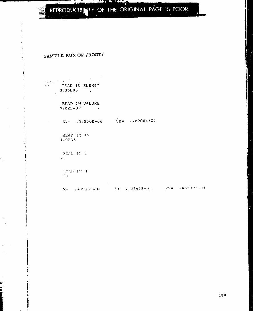
!!
I
SAMPLE RUN OF /ROOT /
':" ".EAD IN ENERGY
3,35E05 ,
RE_D IN VOLUME
7.82E-02
EN= .33500E÷06
READ IN XS
1 • 0 _,_O%
RE_[} I'! E
.I
I )3
.78200E_0!
,12561E-03 FP=
199
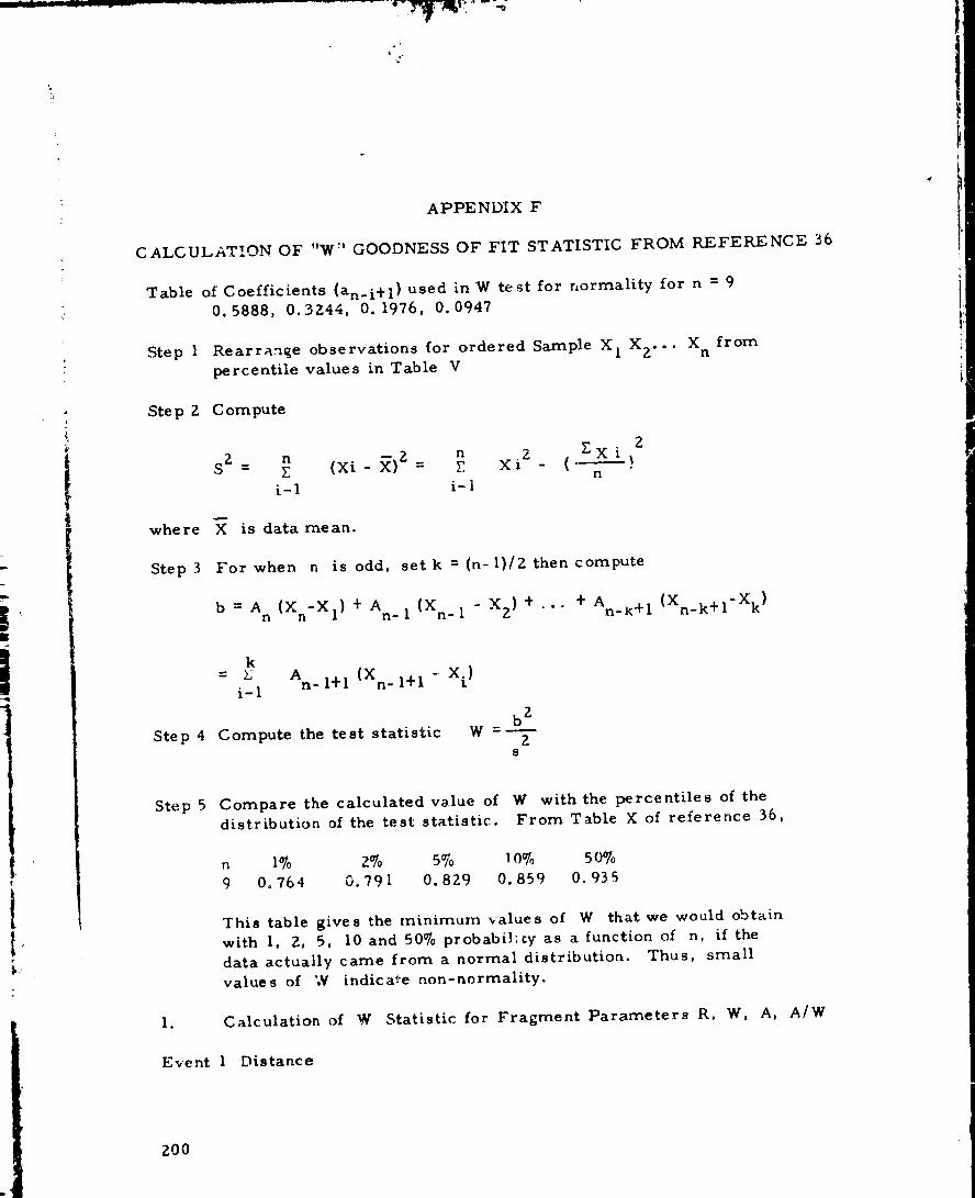
t .
APPENDIX F
CALCULATION OF "W" GOODNESS OF FIT STATISTIC FROM REFERENCE 36
Table of Coefficients (an.i+ I) used in W test for normality for n = 9
0.5888, 0.3Z44, 0. 1976, 0.0947
Step 1 Rearrange observations for ordered Sample X 1 X Z. .. X n from
percentile values in Table V
Step Z Compute
Z
S Z n -- 2 n iZ Z X i %= Z (Xi- X) = _ X - ('--j--.
i-1 i-1
a
where X is data mean.
Step 3 For when n is odd, set k = (n-l)/Z then compute
b = A (Xn-X I) + A (X n - X 2) +n n-I -I+ A k+l (Xn-k+l-Xk)
n-
Step 4
k>: A (X -X.)
n- 1+1 n- 1+1 ti-I
Compute the test statistic W -
Zb
Zs
Step 5 Compare the calculated value of W with the percentiles of thedistribution of the test statistic. From Table X of reference 36,
n 1% z% 5% 10% 50%
9 0.764 0.791 0.8z9 0.859 0.935
This table gives the minimum values of W that we would obtain
with 1, Z, 5, 10 and 50% probabil;cy as a function of n, if the
data actually came from a normal distribution. Thus, small
values of W indica_e non-normality.
1. Calculation of W Statistic for Fragment Parameters R, W, A, A/W
Event I Distance
ZOO
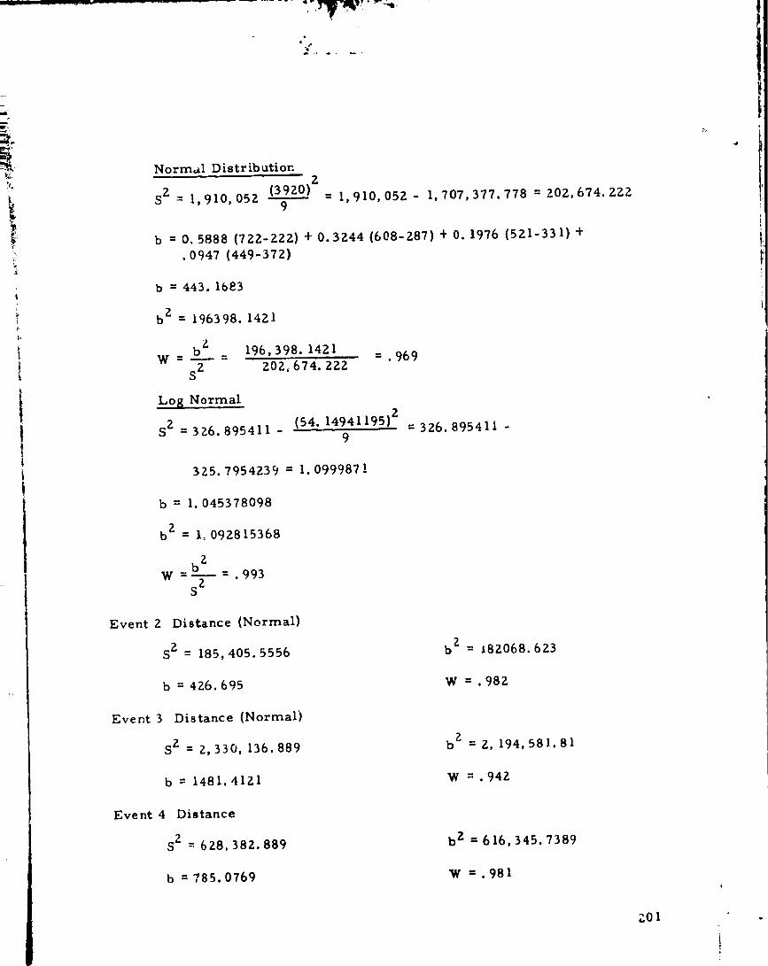
i ,
C
Norm_l Distribution
S2 = 1 910,052 (3920)2' 9
--1,910,052 - 1,707,377.778 - 202,674.222
b = 0. 5888 (722-222) + 0.3244 (608-287) + 0. 1976 (521-331) +
•0947 (449-372)
b = 443. 1683
b Z = 196398. 1421
b Z 196,398. 1421W - - = .969
S2 202,674. 222
Log Normal
SZ =326.895411 -(54. 14941195) Z
9= 326. 895411 -
325.7954239 = 1.099987!
b = 1.045378098
b2 = Io092815368
2b
W - -. 993S 2
Event 2 Distance (Normal)
S 2 = 185,405.5556 b z = 182068. 623
b = 426.695W = •982
Event 3 Distance (Normal)
SZ = 2,330, 136. 889 b 2 = Z, 194,581.81
b = 1481. 4121 W = .942
Event 4 Distance
S 2 : 628,382.889
b = 785.0769
b z =616,345.7389
W =.981
Z01

m_
Event 5 Distance
S 2 = 1,748,338. 889
b = 1300. 255
Event 6 Distance
S 2 = 44172
b = 208. 9122
Event 7 Distance (Normal)
S 2 = 47,296
b = Z14. 0407
Event 8 Distance (Normal)
S2 = 38,674. 8889
b = 193. 7642
Event I Weight (LrA Normal)
5 _ = 4. 02243396
b = 1.959105363
Event 2 Weight {Ln Normal)
S 2 = 9. 55743464
b = 3. 0877 10481
Event 3 Weight {Ln Normal)
32 ffi 8. 308249
b " 2.. 808424493
ETent 4 Weight {Ln Normal)
S2 = 5. 4833992
b = 2. 328636257
202
I
b 2 = 1,690,633. 065
W = .967
b 2 = 43644. 3073 1
W = • 988
b 2 = 45813. 42126
W = .969
b 2 = 37,544. 5652
W =.971
b 2 = 3. 838093823
W = • 954
b 2 = 9. 533956014
W = • 998
b 2 = 7. 887248133
W = • 949
b 2 = 5. 422546817
W = • 989
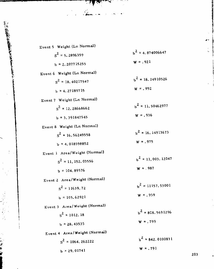
!L
Event 5 Weight (Ln Normal)
S2 = 5. 2896359
b = Z. 2077 15255
Event 6 Weight (Ln Normal)
S 2 = !8. 40217547
b = 4.27 1897 15
Event 7 Weight (Ln Normal)
S z = 12. 28668662
b = 3. 391847545
Event 8 Weight (Ln Normal)
SZ = 16. 56249558
b = 4. 018598852
Event 1 Area/W_ight (Normal)
S 2 = 11, 152.03556
b = 104. 89576
Event Z Area/Weight (Normal)
S 2 = 11639.72
b = 105. 6297.1
Event 3 Azea/Weight (Normal)
S Z = 1012. 18
b = 28. 43535
Event 4 Area/Weight (Normal)
S2 = 1064. 262222
b --'Z9. 01741
b z = 4, 874006647
W = .921
b _ = 18. 24910526
W = .992
b z = II. 50462977
W = •936
bz = 16. 14913675
W = .975
b z = II,003. 12047
W = ,987
b z = 11157.53001
W = •959
b z = 8G8.5691296
W = •799
bz = 842. 0100831
W = .791
Z03

Event 5 Area/Weight (Normal)
S 2 = 515. 8288889
b = 18. 61245
Event 6 Area/Weight (Normal)
S2 = 16338. 98741
b = 126. 724354
Event 7 Area/Weight (Nv..)
S 2 = 11,373.60751
b = 105. 1395562
Event 8 Area/Weight (Normal)
S 2 = 19,558. 42122
b = 138. 6416769
Event 1 Area (Ln Normal)
S 2 = 5. 4012421
t, = 2.3 17066189
Event ?. Area (Ln Normal)
S 2 = 29.313013
b = 5. 322848019
Event 3 Area (Ln Normal)
S 2 = I 1. 8267759
b = 3. 380014318
Event 4 Area (Ln Normal)
S 2 = 11.6117262
b = 3. 350700597
204
b 2 = 346. 423295
W = .672
b 2 = 16059. 6619
W = • 983
b z = 11054. 32628
W = .972
b 2 ffi 19221. 51457
W = • 983
b 2 = 5. 368795724
W = • 994
b 2 = 28. 33271103
W = . 966
b z = !1. 42449679
W = • 966
b Z J 11. 227 194a9
W s .967
#
r
!
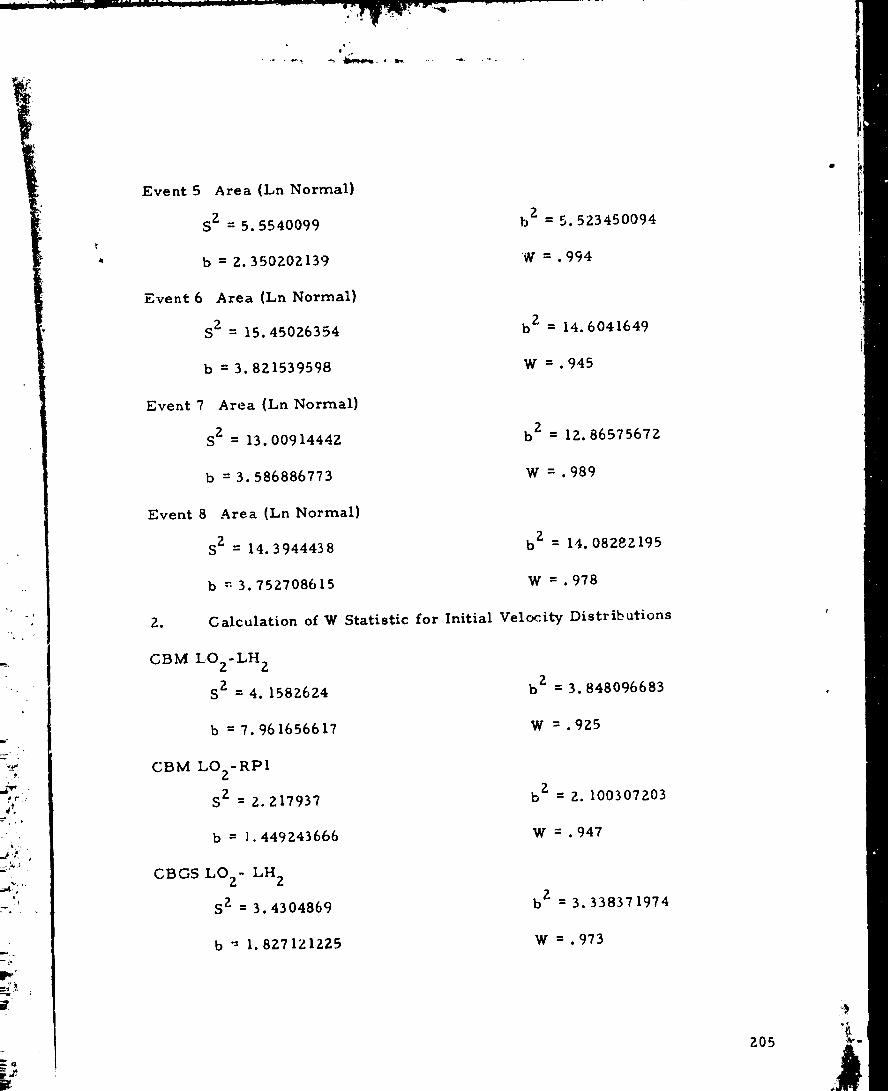
|"
i"
Event 5 Area (Ln Normal)
S 2 = 5. 5540099
b = 2.350202139
Event 6 Area (Ln Normal}
S 2 = 15. 45026354
b = 3. 821539598
Event 7 Area (LnNormal)
S 2 = 13. 00914442
b = 3. 586886773
Event 8 Area (Ln Normal)
S 2 = 14.3944438
1
CBM LOz-LH 2
S2 = 4. 1582624
b = 7. 961656617
CBM LO2- RPI
S 2 = 2.217937
b = ].449243666
CBGS LO z- LH 2
S2 = 3. 4304869
b -- 1.827121225
b2 = 5. 523450094
W" = .994
b 2 = 14.6041649
W = •945
b z = 12.86575672
W = .989
b 2 = 14. 08282195
b - 3. 752708615 W = .978
Calculation of W Statistic for Initial Velocity Distributions
b 2 = 3. 848096683
W = •925
b 2 = 2. 100307203
W = •947
b 2 = 3.338371974
W = .973
205
CBGS LOz-RPl
SZ_.707618
b = 1.299335448
b Z = 1.688Z7Z606
W = .989
m_
m

APPENDIX G
C ALCULATION OF APPROXIMATE PROBABILITY FOR OBTAIhrIING THE
CALCULATED VALUE OF "W"
]_'or n = 9, from Table XI of reference 36, e = -Z. 968, n = I. 400, e = 0. 3900
Approximate probability of obtaining the calculated value of W, assuming a
normally distributed variable can be obtained by finding:
Z = Y+nln - W
Z = -2. 968 + 1.400 in
For W = .94Z
Z = -Z.968 + 1.400 In(.55_ = -Z. 968 + 1.400 In 9.517Z41379
= -Z.968 + 1.400 (Z. Z53105036) = -Z. 968 + 3. 15434705 = • 186347
Pr (Z < 0. 186) = .57
For W =. 994
Z = 3. 4885
Pr = .999
For W = •969
Z=I. I3
Pr = .871
For W = . 954
Z =.54
P = .7054
The following values and table result from using the above methods.
2
,¢
Z07
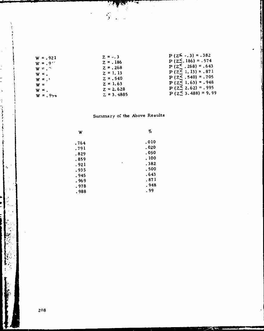
_t
,Bt
f,
W =.921
W=.9 ""
W ._ . "%
W = .
W = ,, _
W =
W =.
W - • 9_
J
4t'.
Z = =..3
Z " • 186
Z = .268
Z=!.13Z " • 540
Z= 1.63Z = Z•628
Z = 3. 4885
P(Z ¢ -.3) =.382
P (Z_<. 186) = . 574P (Z < . 268) = .643
p(Z < I. 13) -" •871
p (Z < . 540) = . 705
p (Z< 1.63) = .948
P (Z < Z.6Z) = . 995
P (Z < 3. 488) = 9.99
Sun_mar_, of the Above Results
.764
•791
• 829
.859
• 9Zl
•935
.945
• 969
• 978
.988
%
.010
.0Z0
• 050
• 100
•382
• 500
.643
.871
• 948
• 99
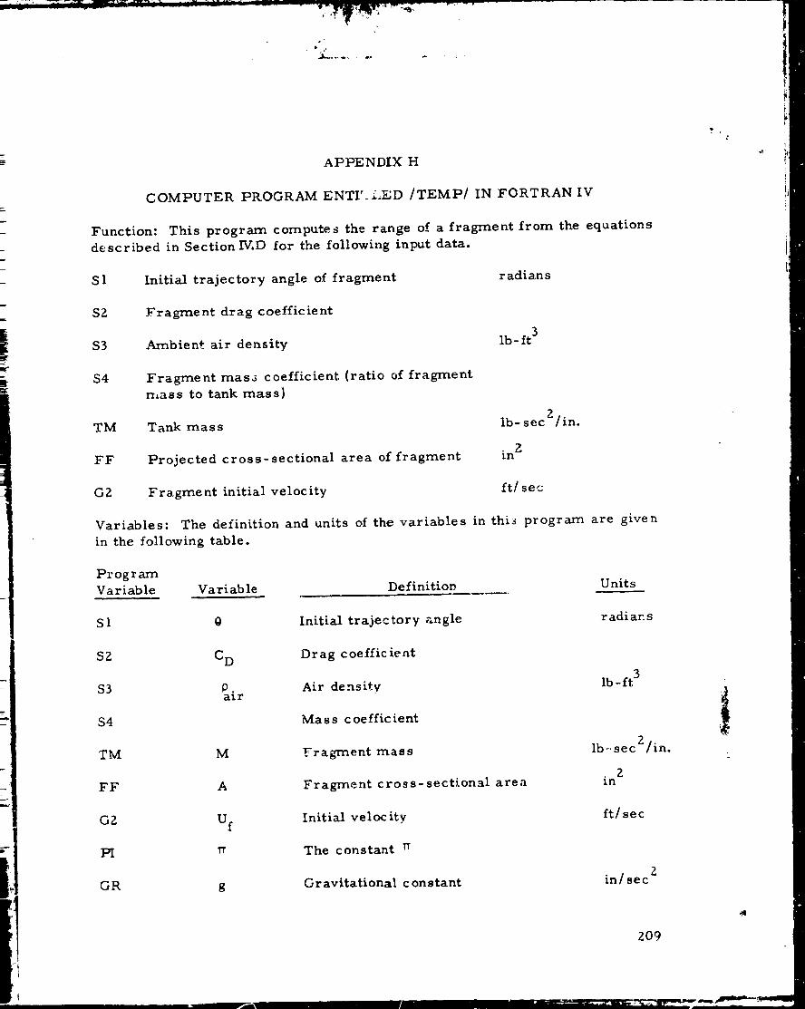
APPENDIX H
COMPUTER PROGRAM ENTI'_i.ED /TEMP/ IN FORTRAN IV
Function: This program computes the range of a fragment from the equations
described in Section IV.D for the following input data.
S1 Initia/ trajectory angle of fragment radians
$2 Fragment drag coefficient
$3 Ambien% air density lb-ft3
$4 Fragment mass coefficient (ratio of fragmentmass to tank mass)
TM Tank mass
ZFF Projected cross-sectional area of fragment in
Zlb-sec /in.
GZ Fragment initial velocity ft/sec
Variables: The definition and units of the variables in this program are given
in the following table.
ProgramVariable Variable Definition Units
SI 0 Initial trajectory angle radians
$2
$3
$4
TM
FF
C D
P.air
M
A
Drag coefficient
Air density
Mass coefficient
Eragment mass
Fragment cross-sectional area
Ib_ft3
lb... sec Z/in.
2in
GZ
Pl
GR
Uf
rr
g
Initial velocity
The constant rr
Gravitational constant
ft/sec
2in/sec
Z09
ProgramVar iable
$5
Variable Definition
The quantity ZA/
Units
Zin
S6 Coefficient defined in Section
IV.D.-I
in
$7
$8
S9
SI0
Sll
S12
VRo
VZO
Initial radial velocity
Initial vertical velocityl/Z
The quantity V (c/g)zO
The quantity tan" 1 V (c / g) I / ZZO
l/ZThe quantity I/ (cg) sec
The quantity cos tan =I Vz ° (c/g)
I/Z
ft/sec
ft/sec
in.
S13
S14
The quantity 2.0 LOG (I.0/S12)
The quantity Z. 0 eS13 - I.0
S15 Time of flight of fragment sec
S16 R Fragment rangeft
TR
ZM
S17
t R
Zm
Time of rise of fragment sec
Maximum height reached by fragment in.
The quantity Z. 0 e Zc Zm - 1.0 sec
TF tf
T
Time of fall of fragment
Time of flight of fraghnent
sec
sec
Sample runs: Substitution of the following data in the program yielded the range
values R {appearing in Figure {,_-I) as X's}. Thus, results of this program
are in accord with Oslake, et al.--
Zl0
i04
6
4
zg
1036
4
2
I I I I I
.uf - 5, _0 ft / sec
uf 1,O00ft/sec -__
uf- ]00 ft/sec
1020 15 30 45 60 75 90
ANGLE OF ELEVATION 0, degrees
FI GU RE HI. FRAGMENT RANGE VERSUS ELEVATION ANGLE
FOR CONSTANT W = I00 LB/FT Z, AND
CONSTANT uf CDA
ZII

I
k"
t,
$it
i
t ,
TABLE H-I - DATA FOR PROGRAM CHECK
SI = 43.3 °
$2= l.Z
$3 =7.48x 10 "2 lb/ft 5
$4 = 1.0
FF = 4.52x 10³ in 2
TM = 6.2 lb-secZ/in.
GZ = 100 ft/sec
500 ft/sec
1000 ft/sec
5000 ft/sec
R = 2.89 x 102 ft
3.19 x 103 ft
5.50 x 103 ft
1.09 x 104 ft
A sample run for the case in which a "mean" fragrr_ent froz,, test 06Z of PYRO
was considered (C D = • 750) is given in the following.
READ IN TRAJo ANGLE
1 2.77
R_A_ IN DRAG CLEF, AN_ AIR DENSITY
.T5,7.aRE-02
I_EAD
1.0
!.0
IN FRAGHENT HASS CeKF.
R_A_ IN Ne. _F FRAGHENT$
FRAG. HAS$
rRAG. PROJ. ARFA
5.77EOR
TNITIAL V_L.
7.4;E0Z
AHR II_,NT AIR DENS ITYm .74_.'01 LRS •/fUR I(" IL"T •
212

AIR nRAG r@_F.= ,750V+_0
_' FkAGM_NT MASS _REF.= .I00_+01
• TR_JECTQRY ANGLE= .128E+0_ _GR_S
722.6715g_a
163.7RgO69R
MAXIMUM _ANGF=
,5_B4E+01
,ST_P*
•353E,+03 FT.
S _'' Y "Z)'IAT
_ 1 F 'S !AT
4/1 .... i'_T
l
• . I
% . ! 'i
TF , ' $'_.
...... I,T
...... "r _ 17i{,; ., , ( -I,
,T ( I, 1 l.(- ( 'I, 1,-D.C
v •
_ = .1'.I : _ ; :",::,
."7 ( ! , 3,l:'l )
( _, _')31 ) ,_1
_ " , i. 3..31 )/(,!.O_,PI)
::I T'
_/,2OH RSAU I_ TRAJ. ANGLE)
E13.5)2/,35.{ lEAD I)_ D._._G CIEF, A._,ID AIR DENSITY)
?;,I3 .,3)_,/, !/_ ':.(AD I)_ =-L:IGIL".'_T IA55 _3F.F. )
ql.,2:,"! S _!DI TI_'.'JS _ TR_.j-CTIRY)
1,21iI ,_.'LIIE_JT A!_ DENSITY=,51(-).3_I?;i
/, 157i AI! _, DRAG CqEF.=+ El0"3)/.-'.if! F.6_3 I.C'IT )IASS C :EF. =, ._I ].'3)
/, 1"_;{ "F._._,jEST3R'f' AhI'3',_L=,EIO.3,S}{ JEGREZS)
31, _;_ CHECk( 0=,"!').3)
(,'_I,1.5;1 I.tXI'4UH ?,;.t•._.':7.=,ElO.3,41t FT,)'¢L_D I_,! _lq. _? F:b_,G'.1S"_T$)
F?,A']. PR!3J • ,,.t;=,'t)v_,,_. lASS)
I IITIAt, ',,;,.L.
( 1, _,()1 )(;j, _ ll I ) ._2,_$3
(l,]c) _.)
(,'),3_)1 ) S.'i
(1,3_.1)
, ,, _3ql ) F"I
Z13
2
i
Y
t
ti
READ (0,3GOI) Tt,I
i"{EAD (0.,3001) F'Ft_:I.ITE ( I , 20_)
READ (0,3001) G2
_4RITE (1,30_) $3_ITE (l,30_) $2'.4RITE (1,306:) S_.
t41_ITE (11,307') SI
$5= (2.0*(FF/PI) )$6= (0.5=( ((S3/GR)*S5*S2)/(Sz_*CTN/FN) ) ) )/(l_.O*o3.0)
'.4RITE (1,3071) 56ST=G2*C_S((2.0*PI)*(SI/360.0))
$8" G2,S IH ( (2.0w.P I )*(SI/3.60.0 ) )
S9= ($8,((S6/GR) **0.5) )*(12.O)
SI 0=ATAN (S 9 )
SI I = ( I. 0/(S6=GR) ) ,s0.5
SI 2= C?'_S(S 10 )313=2.0*AL_G ( I. 0/312)
31 z_= (2.0=}:XP (S 13) )- 1 .0315=S1 I*(.SIO+(0.5=AL;?_G(SI4÷(((SI/4_=2"O)" 1.0)=_,0.5))))
_'RITE (1.,3001) 515S16=(I .9/S6)*AL_3(I.0+(S6"$7"SI_5*12"0))
_1_,=S16/12.0t_IT:L (1,333) 51,,5
T:!= ._ I I :-, tT_,", _( $9 )
'!=(1 ._;/fi--,)*AL:'_G(I.0/C,'3S(TR/SI 1))._I 7= ( 2.3,P:XP (2. O,S6,I,H) )- I. 0
TF=0.5*S1 I,_AL_3G(317+(((SIT**2.0)'I'0)**0"5))
T=TF÷T:I
"_ITE (1,3331) T
i::'J D
ZI4
¢ o
.)
t.
I
Symb ol
a, flO
a,b, c, d
b
d, D, Do
dc A' dCB
g
h
he
k
n, N, NO
Po' Poo
q
r
t, T, T i,
U)U
U.,I
APPENDIX I
LIST OF SYIVIBOLS
Definition
Sound speed
Parameters in a __._ath model
Units
-ILT
Time constant of blast wave
DiametersL
Distances to cameras
Acceleration of gravity, nondimensional
dis plac eme nt
Convective heat transfer coefficient, segment
height
Height of explosion center
Discharge coefficient, constant in fragment
drag equation
Generic length
L
LT =Z, _ _=
MT-30- I, L
L
__.,ML -3
L
Numbers of fragments
Ambient pressure
Drag pressure
Displacement of a fragment
Times
FL -Z
FL -Z
L
T
-IU, U I, LT
s' VelocitiesU U
A' nl
* Units used are force (F), length (L), mass (M), time (T) and temperature (0},
rather than dimensions in any particular physical _vstem.
,*,_ A dash in the units column indicates a dirnensionl" ss quantity,
ZI5

°.
Q .
Symbol
W
x
xi' Yi
Y
A,A,I
C
CD
E
F
G., G.'I 1
H H R ,e' HTNT
Hf.i
I
I, Id
K.
1
L
M,M L'MT
P,P ,Qr
R
Rl
S.
1
T
Definition
C rack width
Mixing function
Coordinates of fragments
Yield Fraction
Areas
Mass of explosive charge or confined _a3
Drag coefficient
Energy of reactant,_
Projected area of a fragment
Dir.,ensional parameters fixed by nondimen-
sional groups
Heats of explosion
Heats of fusion
Heats of boiling
Blast wave impu1_.es
The rmal conductivitie s
Tank length
Masses
Peak pressures
Distance from accident
Universal gas constant
Dis placements
Temperature
Units*
L
L
L z
M
FL
9
various
L z T "Z
L Z T -Z
Z -Z£ T
-ZFTL
MLT'" 3 _- I
L
M
-ZFL
L
LZT- Z @- I
L
t
Z16
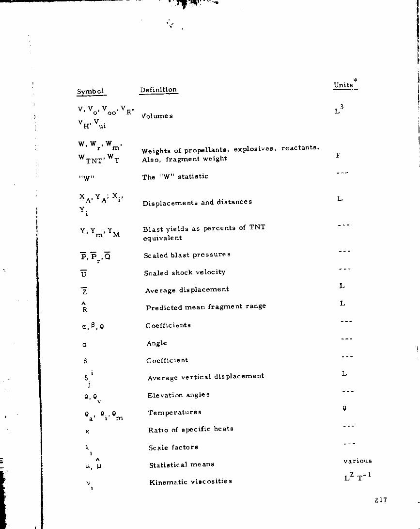
S_b o!
V, V o, Voo, V R,
V H, Vui
Definition
Volume s
Units
L 3
W, W r, W ,m
WTN T, W T
l!wll
Weights of propellants, explosives, reactants.
Also, fragment weight
The "W" statistic
F
XA' YA; Xi'
Y.l
Y'Y 'YMm
P, P ,Qr
U
Z
A
R
a,, 8, 0
CL
5J
0,0v
O Oi,,Oa t I'n
K
),i
^
U, U
Vi
Displacements and distances
Blast yields as percents of TNT
eq uivale nt
Scaled blast pressures
Scaled shock velocity
Ave rage dis placement
Predicted mean fragment range
Coefficients
Angle
C oefficient
Average vertical displacement
Elevation angle s
Temperatures
Ratio of specific heats
Scale factors
Statistical me ans
Kinema.tic viscos ities
L
IJ
L
0
various
LZ T-l
Z17
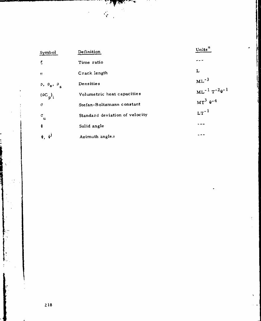
2_
!
|!
Symb ol
g
TI
P, P,,
(pCp)_
O"
U
1
@, *J
ZI8
0S
Definition
Time ratio
Crack length
De ns ities
Volumetric heat capacities
Stefan-B oltzmann constant
Standard deviation of velocity
Solid angle
Azimuth angle ,_
Units*,l
L
ML-3
ML-1 T-Z0- 1
MT 3 0-4
-ILT

.
Zo
)
o
.
.
o
o
.
10.
REFERENCES
Baker, Wilfred E., E_x_losions in Air, Univ. of Texas Press,
Austin, Texas, May 1973.
Kingery, C. N. andB. F. Pannill, "Peak Overpressure vs.Scaled Distance for TNT Surface Burst (Hemispherical Charges)",
DRL Memo Report No. 1518, Aberdeen Proving Ground, Md.,
April 1964. AD 443 10e
Carter, P. B., Jr., "A Method of Evaluating Blast Parameters
Resulting from Detonation of Rocket Propellants", AEDC-TDR-
64-200, Arnold Engineering Dev. Center, Air Force Systems
Command, Oct. 1964. AD 450140
Gurney, R. W., _'The Initial Velocities of Fragments from Bombs,
Shells, and Grenades," BRL Report 405, 1943.
Henry, I. G. , "The Gurney Formula and Related Approximations
for the High-Explosive Deployment of Fragments, " Hugkes
Aircraft Company, Report No. PUB-189, Culver City, California,
April 1967.
Ahlers, E. B. , "Fragment Hazard Study, " Minites of the Eleventh
Explosives Safety Seminar, September 1969, pp. 81-107.
Gwaltney, R. C., "Missile Generation and Protection in Light-
Water-Cooled Power Reactor Plant, " ORNL-NSIC-Z2, Oak
Ridge National Laboratory, September 1968.
Gates, R. W., "Containment of Fragments from a Runaway Reactor,
Stanford Research Institute, Menlo ParK, California, SRIA-I17
AEG ResearcL and Development Report UC-80, Reactor Technology
TID-4500 (27thEdition), February 1S, 1964. Final Report prepared
for U. S. Atomic Energy Commission, Contract No. AT(04-3)- 115,
Project Agreement No. 2.
Proceeding13 of the Second United Nations International Conference
ou Peaceful Uses of Atomic Ener_., Vol.
Control, United Nations, Geneva, 1958.
11, Reactor Safety and
Brittan, R. O. and J. C. Heap,
in Ref. 9.
"Reactor Containment, " pp. 66-78
Z 19
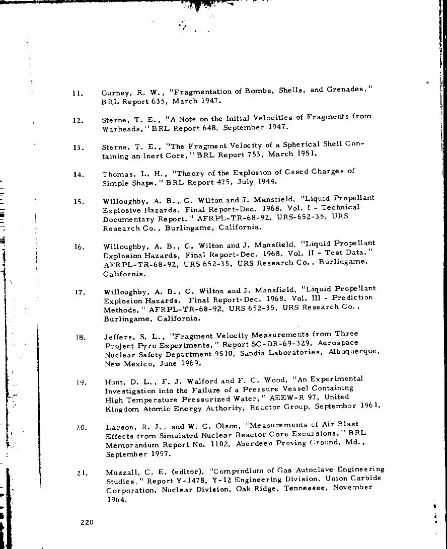
11.
1Z.
13.
14.
15.
16.
17.
18.
19.
Z0.
gl.
Gurney, R. W., "Fragmentation of Bombs,BRL Report 635, March 1947.
Shells, and Grenades,
Sterne, T. E., "A Note on the Initial Velocities of Fragments from
Warheads,"BRL Report 648, September 1947.
Sterne, T. E. , "The Fragment Velocity of a Spherical Shell Con-
taining an Inert Core,"BRL Report 753, March 1951.
Thomas, L. H., "Theory of the Explosion of Cased Charges of
Simple Shape, " BRL Report 475, July 1944.
Willoughby, A. B. ,. C. Wilton and J. Mansfield, "Liquid Propellant
Explosive Hazards. Final Report-Dec. 1968. Vol. I - Technical
Documentary Report," AFRPL-TR-68-92, URS-652-35, URS
Research Co., Burlingame, California.
Willoughby, A. B., C. Wilton and J. Mansfield, "Liquid Propellant
Explosion Hazards, Final Report-Dec. 1968. Vol. II - Test Data,"AFRPL-TR-68-92, URS 652-35, URS Research Co., Burlingame,
California.
Willoughby, A. B., C. Wilton and J. Mansfield, "Liquid Propellant
Explosion Hazards. Final Report-Dec. 1968. Vol. III- PredictionMethods," AFRPL-TR-68-92, URS 652-35, URS Research Co.,
Burlingame, California.
Jeffers, S. L., "Fragment Velocity Measurements from Three
Project l_,ro Experiments," Report SC-DR-69-3Z9, AerospaceNuclear Safety Department 9510, Sandia Laboratories, Albuquerque,
New Mexico, June 1969.
Hunt, D. L., F. J. Walford and F. C. Wood, "An Experimental
Investigation into the Failure of a Pressure Vessel Containing
High Temperature Pressurized Water," AEEW-R 97, United
Kingdom Atomic Energy Authority, Reactor Group, September 1961.
Larson, R. J.. and W. C. Olson, "Measurements c,f Air Blast
Effects from Simulated Nuclear Reactor Core Excursions, " BRL
Memorandum Report No. 1102, Aberdeen Proving (round, Md.,
September 1957.
Muzzall, C. E. (editor), "Compendium of Gas Autoclave Engineering
Studies," Report Y-1478, Y-I?- Engineering Division, Union Carbide
Corporation, Nuclear Division, Oak Ridge, Tennessee, November
1964.
220
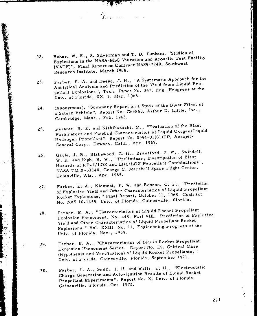
ZZ.
Z3.
Z4.
Z5,
Z6.
Z7°
Z8.
Z9.
30.
Baker, W. E., S. Silverrnan and T. D. Dunham, "Studies of
ExFlosions in the NASA-MSC Vibration and Acoustic 'rest Facility
(VATF)", Final Report on Contract NAS9-7749, Southwest
Research Institute, March 1968.
Farber, E. A. and Deese, J. H., "A Systematic Approach for the
Analytical Analysis and Prediction of the Yield from Liquid Pro-
pellant Explosions", Tech. Paper No. 347, Eng. Progress at the
Univ. of Florida, X__X, 3, Mar. 1966.
(Anonymous), "Summary Report on a Study of the Blast Effect of
a Saturn Vehicle", Report No. C63850, Arthur D. Little, Inc.,
Cambridge, Mass., Feb. 1962.
Pesante, R. E. and Nishibazashi, M., "Evaluation of the Blast
Parameters and Fireball Characteristics of Liquid Oxygen/Liquid
Hydrogen Propellant", Report No. 0954-01(01)FP, Aerojet-
General Corp., Downey, Calif., Apr. 1967.
Gayle, J. B., Blakewood, C. H., Bransford, J. W., Swindell,
W. H. and High, R. W., "Preliminary Investigation of Blast
Hazards of RP-I/LOX and LHz/LOX Propellant Combinations",
NASA TM X-53Z40, George C. Marshall Space Flight Center,
Huntsville, Ala., Apr. 1965.
Farber, E. A., Klement, F. W. and Bonzon, C. F., "Prediction
of Explosive Yield and Other Characteristics of Liquid Propellant
Rocket Explosions," Final Report, October 31, 1968, Contract
No. 1NAS 10-1255, Univ. of Florida. Gainesville, Florida.
Farber, E. A., "Characteristics of Liquid Rocket Propellant
Explosion Phenomena. No. 448. Part VIII. Prediction of Explosive
Yield and Other Characteristics of Liquid Propellant Rocket
Explosions," Vol. XXHI, No. 11, Engineering Progress at the
Univ. of Florida, Nov., 1969.
Farber, E. A., "Characteristics of Liquid Rocket Propellant
Explosion Phenomena Series. Report No. IX. Critical Mass
{Hypothesis and Verification) of Liquid Rocket Propellants, "Univ. of Florida, Gainesville, Florida, September 1971.
Farber, E. A., Smith, J. H. and Watts, E. H , "Electrostatic
Charge Generation and Auto-ignition Results of Liquid Rocket
Propellant Experiments", Report No. X, Univ. of Florida,
Gainesville, Florida, Oct. 1972.
ZZl
J
31.
3Z.
33.
34.
35.
36.
37.
38.
39.
40.
41.
42.
43.
Taylor, D. B. and C. F. Price, "Velocities of Fragment From
Bursting Gas Reservoirs," ASME Transactions, Journal of
EnGineering for Industry, Nov. 1971.
Grodzovski, G. L., and F. A. Kukanov, "Motion of Fragments of
a Vessel Bursting in a Vacuum, " Soviet Engineerin 8 Journal,
Mar/Apr 1965.
Pittman, J. F., "Blast and Fragment Hazards From Bursting
High Pressure Tanks," NOLTR 72-102, May 1972.
Glasstone, Samuel, The Effects of Nuclear Weapons, U. S.
Government Printing Office, Revised Edition, April 1962.
Hoerner, Sighard F. , Fluid-Dynamic Drag, Published by the
Author, Midland Park, New Jersey, 1958.
Hahn, Gerald J. and Shapiro, Samuel S., Statistical Models in
Engineering, John Wiley and Sons Inc., New York, 1967.
Fletcher, R. F., "Liquid-Propellant Explosions", Jour. of Space-
craft and Rockets, 5, 10, pp 1227-1229, Oct. 1968.
(Anonymous), SIV All Systems Vehicle :Malfunction 24 January
1964, Douglas Missile & Space Division, Santa Monica, California.
Deese, J. H., Test Conductors Damage Assessment Report on
Auto-Ignition L02/LHZ Mixing Test Experimental Expersion of
2 March 1972, S/stems Engineering Division, Kennedy Space
Center, NASA.
Dixon, W. J., Biomedical Compute:" Programs, University of
California Press, Los Angeles, C_lifornia 1970.
Oslake, J. J., Getz, R. J., Romine, R. A. and Sooftov, K.,
"Fxplosive Hazards of Rocket Launchings, " Ford Motor Co.
Technical Report 4-108:98, Nov. 1960, AD253-235.
Heppner, L. D. and Steedman, J. E., "Drag Coefficient for
Fragment Simulating Projectiles, 2.0 MM, Caliber . 50, andCaliber .30," APG DPS-286, Aug. 1961, AD 822-489.
Richards, E., "Comparative Dispersion and Drag of Spheres and
Light Cylinders," APG BRL TR-717, March 1950.
ZZZ

44.
45.
46.
47.
48.
7. _, ..
Feinstein, D. I., "Fragmentation Hazards to Unprotected Personnel"
TR rrTRI-J6176 January 197Z.
Transue, W. R. and Saramel, K. M., "Terminal Ballistics-
Fragmentation Effects, " TR Institute of Research Lehigh University,
December 1947.
thomas, J. H., "Computing Effect ef Distance on Damage by
Fragments" APG-BRL Report No. 468, May 1944.
Lewz, H., "Asymptotic Integration of Fragment Trajectories"
APG-BRL Report No. 559 and Technical Note No. 496, September
1951.
Feinstein, D. I. and Nazooka, H. H., "Fragment Hazards From
Detonation of Multiple Munitions in Open Stores, " TR IITRI-J6176,
August 1971.
ZZ3
/
Q